Regret Analysis of the Stochastic Direct Search Method for Blind Resource Allocation

Abstract

Motivated by programmatic advertising optimization, we consider the task of sequentially allocating budget across a set of resources. At every time step, a feasible allocation is chosen and only a corresponding random return is observed. The goal is to maximize the cumulative expected sum of returns. This is a realistic model for budget allocation across subdivisions of marketing campaigns, when the objective is to maximize the number of conversions.

We study direct search (aka pattern search) methods for linearly constrained and derivative-free optimization in the presence of noise. Those algorithms are easy to implement and particularly suited to constrained optimization. They have not yet been analyzed from the perspective of cumulative regret. We provide a regret upper-bound of the order of $T^{2/3}$ in the general case. Our mathematical analysis also establishes, as a by-product, time-independent regret bounds in the deterministic, unconstrained case. We also propose an improved version of the method relying on sequential tests to accelerate the identification of descent directions.

Keywords— online learning, regret minimization, derivative-free optimization, direct search.

1 Introduction

1.1 Motivation

In the field of programmatic marketing advertisement, advertisers are given daily budgets that they are required to entirely distribute across a number of predefined subdivisions of a campaign. Their goal is to maximize some notion of cumulative reward on the lifetime of the campaign, corresponding to the number of clicks or purchases generated by the campaign. We posit that the expected reward generated by each subdivision every day is an unknown function of the daily budget allocated to that campaign. We focus on the context in which, when choosing a specific allocation, the advertiser only observes a noisy version of the total reward. The optimization task faced by the advertiser can thus be formalized as a continuous resource allocation problem, under zeroth order and noisy feedback. Indeed, a key operational constraint in this field is the impossibility to directly access higher-order (derivative) information. Furthermore, every noisy evaluation of the objective function has a cost, related to the value of the function, that needs to be accounted for in the performance criterion. In this context, the cumulative reward is thus more relevant than alternative traditional measures of performances based, for instance, on the distance to the optimum or the norm of the gradient of the objective function reached after some iterations.

1.2 Model

Let us assume that the learner has access to $d+1\in\mathbb{N}$ different resources. To keep up with the dominant convention in optimization, we will consider a minimization problem for which the costs may be thought of as minus the rewards. At each round $t\in\{1,\ldots T\}$, the learner is allowed to choose the level of consumption that she makes of each resource, on a continuous scale from $0$ to $1$. We impose that the consumption levels of all the resources sum to $1$. The use of resource $i\in\{1,\ldots,d+1\}$ to a level of $x_{t}^{(i)}$ generates an expected marginal cost $w_{i}(x_{t}^{(i)})$. Overall, the expected one-step cost of the learner is given by $\sum_{i=1}^{d+1}w_{i}(x_{t}^{(i)})$, where the set of all possible consumption levels $(x_{t}^{(1)},\ldots,x_{t}^{(d+1)})$ correspond to the $d$ dimensional simplex. The goal of the learner is to sequentially minimize the expected cumulative cost over $T$ evaluations of the function, having access only to a noisy version of the expected cost associated to the allocation tried at step $t$. Not only are the cost functions $w_{1}$ to $w_{d+1}$ unknown, but one cannot observe their individual outputs. Although we are primarily motivated by resource allocation, the algorithms studied in this paper may be applied to more general linearly-constrained optimization problems, and their analysis holds in the general case. In the remainder of the paper, we thus consider a generic optimization domain $\mathcal{D}$ that is a subset of $\mathbb{R}^{d}$ defined by linear constraints: $\mathcal{D}=\{x\in\mathbb{R}^{d},A_{I}x\leq u\}$ with $m\in\mathbb{N}$, $A_{I}\in\mathbb{R}^{m\times d},$ and $u\in\mathbb{R}^{m}$. At each round $t\in\{1,\ldots T\}$, the learner selects $x_{t}\in\mathcal{D}$ and incurs a cost $f(x_{t})+\epsilon_{t}$, where $\epsilon_{t}$ is assumed to be a centered $\sigma$-subgaussian noise, with $\sigma$ known to the learner.

The goal of the learner is to minimize the cumulative cost over $T$ evaluations of the function, or equivalently to minimize the cumulative regret

$$R_{T}=\sum_{t=1}^{T}f(x_{t})-f(x_{\star})\;,$$

where we denote by $x_{\star}\in\mathcal{D}=\operatorname*{arg\,min}_{x\in\mathcal{D}}f(x)$ the optimal allocation. We make the following regularity assumptions on $f$.

Assumption 1.

$f$ is continuously differentiable, $\beta$-smooth and $a$-strongly convex on $\mathcal{D}$.

We highlight that if $f$ satisfies Assumption 1 then $f$ has a unique minimum and is bounded from below. Assumption 1 is arguably restrictive but common in online optimization due to the difficulty of controlling the cumulative cost without this assumption.

Assuming convexity of $f$ on $\mathcal{D}$ is reasonable for budget allocation, because in programmatic advertising and economics more generally, one commonly observes that the marginal return associated to each resource is diminishing with the level of the resource (following the so-called law of diminishing returns). Indeed, Assumption 1 implies that when $f$ has the form $f(x_{t}^{(1)},\ldots x_{t}^{(d)})=\sum_{i=1}^{d}w_{i}(x_{t}^{(i)})+w_{d+1}\left(1-\sum_{i=1}^{d}x_{t}^{(i)}\right)$, the marginal cost functions $w_{1}$ to $w_{d+1}$ are also convex and hence satisfy the law of diminishing return (viewing $-w_{i}$ as the marginal utility associated to the $i$-th ressource).

In this paper, we propose to extend the analysis of direct search methods to the optimization of regular functions. Direct search [Kolda et al., 2003], also known as pattern search, makes use of the well-known fact that if the objective function is continuously differentiable, then at least one of the directions of a positive spanning set (a set that spans the space with non-negative coefficients, abbreviated as PSS in what follows) is a descent direction. It explores the space by testing new points in a number of predefined directions from the current iterate but at a distance that varies with time. The algorithm moves to a new iterate only if it results in a sufficient improvement of the value of the function (there exist other versions of the algorithm where the sufficient decrease condition is replaced by a constraint on the choice of the trial directions). The complexity of such an algorithm has been analyzed in [Vicente, 2013] in the deterministic and unconstrained setting. Lewis and Torczon [2000] study direct search in linearly constrained domains. Handling the constraints in direct search is quite simple, as it consists in testing only the directions in the set of search-directions that are feasible. Gratton et al. [2015] analyzed direct search with random sets of search-directions instead of predefined ones and later extended the analysis to the case of linearly-constrained domains [Gratton et al., 2019]. Dzahini [2022] extended their work by analyzing a similar algorithm in the presence of noise, but without constraints. Dzahini [2022] relies on an assumption on the decrease of the noise. In this paper, we will study direct search algorithms that rely on a number of samples at each point to build tight estimates of the function at the trial points, which can be understood as a way to decrease the noise. Dzahini [2022] analyzes some notion of sample complexity of direct search, which only takes the iterates into account rather than the number of function evaluations needed, which is not fully appropriate in our setting.

1.3 Contributions

Our purpose is to study methods that are suitable for the blind resource allocation model. We choose to study extensions of the direct search algorithm for the optimization of regular functions in the presence of linear constraints and noise. The adaptation of direct search to the noisy case is achieved by performing enough sampling to ensure that the algorithm moves to a new iterate only if it results in a sufficient improvement, with high probability. We propose two ways of doing so: the first method (termed FDS-Plan) simply computes the number of necessary evaluations ahead of time, whereas the second one, FDS-Seq, uses a sequential testing strategy to interrupt sampling as early as possible. The algorithms are specified in Section 2. We analyze the cumulative regret of these algorithms in Section 3, providing an upper bound of their regret of the order of $T^{2/3}$ (up to logarithmic factors), when the optimum is in the interior of the feasible domain. We start Section 3 by the simpler case in which there is neither noise nor constraints, showing that in this basic setup the regret of direct search is bounded by a constant.

2 Algorithms

2.1 Description of the Algorithms

In Algorithm 1 below, we start by describing the most common version of the direct search method, used for deterministic and unconstrained optimization. It requires the setting of an initial point $x_{0}$ and an initial parameter $\alpha_{0}$. The learner also specifiesa PSS $\mathbb{D}$, that is, a set of directions that spans $\mathbb{R}^{d}$ with non-negative coefficients. At each iteration, the algorihtm sequentially tests points at a distance $\alpha_{k}$ from the current iterate and in the directions defined by $\mathbb{D}$. If none of the test points results in a sufficient decrease of the function’s value, the iteration is declared unsuccessful and the trial radius $\alpha_{k}$ shrinks by a factor $\theta<1$, otherwise, the iteration is declared successful and the iterate $x_{k}$ is moved to the first trial point that results in a sufficient improvement. A decrease is considered to be sufficient if it is larger than some predefined forcing function of $\alpha_{k}$, that we take here to be quadratic, with a coefficient that can be set by the learner.

1Choose $x_{0}\in\mathbb{R}^{d}$, $\alpha_{0}>0$, $\theta\leq 1$, $c>0$, $\rho(u)=cu^{2}$ and a PSS $\mathbb{D}$

2 for $k=0\ldots K$ do

3       Set UnsuccessfulSearch $\leftarrow$ True

4       for $v\in\mathbb{D}$ do

5             Evaluate $f(x_{k}+\alpha_{k}v)$

6             if $f(x_{k})-f(x_{k}+\alpha_{k}v)\geq\rho(\alpha_{k})$ then

7                   Set $x_{k+1}\leftarrow x_{k}+\alpha_{k}v$ and $\alpha_{k+1}\leftarrow\alpha_{k}$

8                   Set UnsuccessfulSearch $\leftarrow$ False

9                   break

10      if UnsuccessfulSearch then

11             Set $x_{k+1}\leftarrow x_{k}$ and $\alpha_{k+1}\leftarrow\theta\alpha_{k}$

Algorithm 1 Direct Search with sufficient decrease

The analysis can also be adapted to the presence of a growth factor $\gamma\geq 1$ by which the trial radius $\alpha_{k}$ expands at successful iterations. To simplify, we choose to focus on the case where $\gamma=1$, as this parameter does not modify the regret rates obtained in Section 3. Also note that Algorithm 1 is a descent algorithm with respect to the iterates $x_{k}$, I.e., the sequence $(f(x_{k}))_{k}$ is decreasing.

It is obvious that different choices of PSS result in different trajectories of the algorithm. A common choice of $\mathbb{D}$ as the set of $2d$ vectors of the positive and negative coordinate directions results in the algorithm known as coordinate or compass search. Other frequently considered choices include random directions, as in [Gratton et al., 2015, 2019, Dzahini, 2022].

We apply two sorts of modifications to Algorithm 1 in order to adapt it to the more general model introduced in Section 1.2. The first modification consists in sampling a trial point only if it is feasible. The second modification consists in introducing estimation stages that allow building reliable estimates of $f$ at the trial points. We propose two ways of doing so, that result in two different algorithms. The first algorithm that we study is a plug-in version of Algorithm 1 in which we replace $f(x_{k})$ and $f(x_{k}+\alpha_{k}v)$ by their empirical estimates, consisting of means computed from $N_{k}=\frac{32\sigma^{2}\log(2/\delta)}{\rho(\alpha_{k})^{2}}$ samples. This number of samples guarantees that with high probability, the estimation gap is smaller than $\rho(\alpha_{k})/4$, which in turn ensures that an iteration is declared successful only when it leads to a decrease of $f(x_{k})$ by at least $\rho(\alpha_{k})/2$ and that an unsuccessful iteration cannot occur if there exists a direction $v$ in $\mathbb{D}$ such that the decrease achieved by moving to $x_{k}+\alpha_{k}v$ is larger than $3\rho(\alpha_{k})/2$. The resulting algorithm is termed Feasible Direct Search with a planned number of Samples (FDS-Plan) and described in Algorithm 2.

1Choose $x_{0}\in\mathbb{R}^{d}$, $\alpha_{0}>0$, $\theta\leq 1$, $c>0$, $\rho(u)=cu^{2}$ and a PSS $\mathbb{D}$

2 for $k=0\ldots K$ do

3       Set UnsuccessfulSearch $\leftarrow$ True

4       Set $N_{k}=\frac{32\sigma^{2}\log(2/\delta)}{\rho(\alpha_{k})^{2}}$.

5       Estimate $f(x_{k})$ by making $N_{k}$ samples at $x_{k}$ and setting $\hat{f}(x_{k})=\frac{1}{N_{k}}\sum_{j=1}^{N_{k}}f(x_{k})+\epsilon_{j}$

6       for $v\in\mathbb{D}$ such that $x_{k}+\alpha_{k}v\in\mathcal{D}$ do

7             Estimate $f(x_{k}+\alpha_{k}v)$ by making $N_{k}$ samples at $x_{k}+\alpha_{k}v$ and setting $\hat{f}(x_{k}+\alpha_{k}v)=\frac{1}{N_{k}}\sum_{j=1}^{N_{k}}f(x_{k}+\alpha_{k}v)+\epsilon_{j}^{\prime}$

8             if $\hat{f}(x_{k})-\hat{f}(x_{k}+\alpha_{k}v)\geq\rho(\alpha_{k})$ then

9                   Set $x_{k+1}\leftarrow x_{k}+\alpha_{k}v$ and $\alpha_{k+1}\leftarrow\alpha_{k}$

10                   Set UnsuccessfulSearch $\leftarrow$ False

11                   break

12      if UnsuccessfulSearch then

13             Set $x_{k+1}\leftarrow x_{k}$ and $\alpha_{k+1}\leftarrow\theta\alpha_{k}$

Algorithm 2 Feasible Direct Search with Planning (FDS-Plan)

We also propose a faster algorithm, Feasible Direct Search with Sequential Tests (FDS-Seq) described in Algorithm 3. For any $v\in\mathbb{D}$, instead of planning the number of samples at $x_{k}+\alpha_{k}v$ ahead of time, it samples at $x_{k}+\alpha_{k}v$ and $x_{k}$ until either

$$\begin{cases}\left|\hat{f}_{n_{0,k}}(x_{k})-\hat{f}_{n_{v,k}}(x_{k}+\alpha_{k}v)-\rho(\alpha_{k})\right|\leq\sqrt{2\sigma^{2}\log(1/\delta)\Big{(}\frac{1}{n_{0,k}}+\frac{1}{n_{v,k}}\Big{)}}\;,\\ \text{or }\left(n_{0,k}\geq N_{k}\text{ and }n_{v,k}\geq N_{k}\right)\;,\end{cases}$$ (1)

where $n_{0,k}$ and $n_{v,k}$ denote the number of samples at $x_{k}$ and $x_{k}+\alpha_{k}v$ and $\hat{f}_{n_{0,k}}(x_{k})$ and $\hat{f}_{n_{v,k}}(x_{k}+\alpha_{k}v)$ denote the resulting empirical means. Then, successful and unsuccessful iterations are defined as in FDS-Plan, and lead to the same actions.

The sequential stopping rule is designed to achieve early detection of sufficient decrease, but also to detect as early as possible the cases in which the trial point cannot lead to a sufficient decrease. The first test in Condition (1) is a consequence of the fact that the estimation gap at $x_{k}$ (respectively $x_{k}+\alpha_{k}v$) is $\sigma^{2}/n_{0,k}$ subgaussian (respectively $\sigma^{2}/n_{v,k}$ subgaussian). The second test of Condition (1) corresponds to a safeguard that prevents from waiting too long in cases where the decrease induced by the trial point is very close to the sufficiency threshold. At worst, the number of evaluations needed is the same as in Algorithm 2. Essentially, the sequential stopping rule reduces the number of evaluations needed for each iteration but maintains the desirable property that with high probability, an iteration is declared successful only if it leads to a decrease of at least $\rho(\alpha_{k})/2$ and that an iteration cannot be declared unsuccessful if there exists a direction $v$ in $\mathbb{D}$ such that the decrease achieved by moving to $x_{k}+\alpha_{k}v$ is larger than $3\rho(\alpha_{k})/2$.

1 Choose $x_{0}\in\mathbb{R}^{d}$, $\alpha_{0}>0$, $\delta>0$, $\theta\geq 1$, $c>0$, $\rho(u)=cu^{2}$ and select a PSS $\mathbb{D}$

2 Set UnsuccessfulSearch $\leftarrow$ True

3 for $k=0\ldots K$ do

4       for $v$ in $\mathbb{D}$ such that $x_{k}+\alpha_{k}v\in\mathcal{D}$ do

5             while Condition (1) is not satisfied  do

6                   if $n_{v,k}\leq n_{0,k}$ then

7                        Sample at $x_{k}+\alpha_{k}v$ and update $n_{v,k}$ and the empirical mean $\hat{f}_{n_{v,k}}(x_{k}+\alpha_{k}v)$.

8                  else

9                        Sample at $x_{k}$ and update $n_{0,k}$ and the empirical mean $\hat{f}_{n_{0,k}}(x_{k})$

10            if $\hat{f}_{n_{0,k}}(x_{k})-\hat{f}_{n_{v,k}}(x_{k}+\alpha_{k}v)\geq\rho(\alpha_{k})$  then

11                  Set $x_{k+1}\leftarrow x_{k}+\alpha_{k}v$, and $\alpha_{k+1}\leftarrow\alpha_{k}$.

12                   UnsuccessfulSearch $\leftarrow$ False

13                   Break.

14      if UnsuccessfulSearch then

15             Set $x_{k+1}\leftarrow x_{k}$ and $\alpha_{k+1}\leftarrow\theta\alpha_{k}$

Algorithm 3 Feasible Direct Search with Sequential Tests (FDS-Seq)

2.2 Illustration

In order to illustrate graphically the behavior of the proposed methods, we show on Figure 1(a) and 1(d) their trajectories in the case where there are 3 resources ($d=2$) and the loss functions associated to each resource $i\in\{1,\dots,d+1\}$ are of the form $w_{i}(x)=-\tau_{i}\frac{\log(1+\gamma x)}{\log(1+\gamma)}$ with $\gamma=2$, $\tau_{1}=1$, $\tau_{2}=0.45$, and $\tau_{3}=0.95$. We set the horizon to $T=100,000$ and use a Gaussian noise with standard deviation $\sigma=0.1$, a realistic value for budget allocation problems. In the symmetric representation of Figure 1, the three vertices correspond to the points where one of the resource is fully saturated (equal to 1) and the edges to linear paths along which one of the resources is set to 0. The contour lines of the target function are materialized by orange lines and the location of the minimum is marked by a black cross. The size of each point is a logarithmically growing function of the number of samples made at this point, and its color is a function of the index of the first round at which it has been sampled. Finally, points at which a successful iteration of FDS-Plan (respectively FDS-Seq) occurred are circled in blue. The parameters of both versions of feasible direct search are $\alpha_{0}=0.2$, $c=5$ and $\theta=0.7$, and the initial point corresponds to the allocation $x(0)=(1/3,1/3,1/3)$ (center of the simplex). The set of directions chosen for these algorithms are the 6 directions that support the edges of the simplex (in both directions).

In a first phase, the algorithm proceeds rapidly by testing directions until a sufficient descent direction is found. Afterwards, when the iterates get closer to the minimizer, the search area has to iteratively shrink and finding descent directions becomes harder. In the first phase, the trajectory is similar to a descent path that would result from a gradient descent algorithm for example, while the second phase is more reminiscent of the behavior of bandit algorithms based on hierarchical partitions, like HOO [Bubeck et al., 2011]. In order to illustrate the differences with such algorithms, we also plot the trajectories of baseline methods, either related to gradient descent or bandits with hierarchical partitioning. The literature related to these methods is reviewed in details in Section 3.3. Before turning to these other algorithms, it is important to note the difference between FDS-Plan and FDS-Seq. Figure 1(d) shows that FDS-Seq is faster than FDS-Plan, as it spends less time on the first iterations, in which it is easy to determine whether the trial points lead to a sufficient decrease. The FDS-Seq algorithm can thus perform more iterations than FDS-Plan.

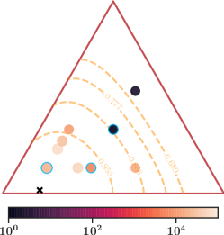
(a) FDS-Plan

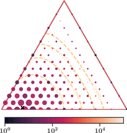
(b) HOO

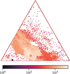
(c) Gradient Descent with two-points estimate

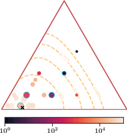
(d) FDS-Seq

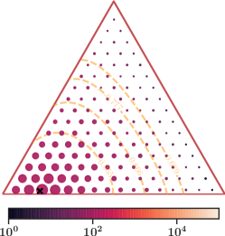
(e) UCB

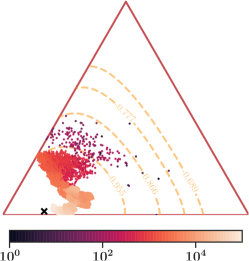
(f) Gradient Descent with one-point estimate

Figure 1: Single trajectories

Let us now comment on Figure 1(b), that represents the trajectory of a version of HOO. It is not straightforward to apply algorithms for $\mathcal{X}-$armed bandits like HOO on the simplex, because it implies constructing balanced hierarchical partitions of the simplex. In the following, the tree of partitions that we used is built in the following way. We set the parameter $\rho$ of HOO as suggested by Bubeck et al. [2011] to $2^{-2/d}$. A binary tree of depth $H=\frac{\log(1/T)}{2\log(\rho)}$ of partitions of $[0,1]^{d}$ is obtained by recursively halving the cells at each depth $h$ of the tree along dimension $h\pmod{2}$. At depth $h$ of the tree, this approach yields a partition formed by rectangular cells represented by their lower left corner $[a_{i},b_{i}]$. Then, in order to remove unwanted cells, we traverse the tree, starting from the leaves, and remove every cell having an empty intersection with the domain. Due to the geometry of the simplex, knowing if a cell intersects the domain boils down to checking if its representant $[a_{i},b_{i}]$ belongs to it. When the algorithm selects cell $(h,i)$ at time $t$, the representant of that cell is chosen as a sampling point. In the simulation, the smoothness parameter $\nu_{1}$ of HOO is set to $16$. On Figure 1(b), we observe that this algorithm explores the partition tree in a way that favors the cells close to the optimum while persistently visiting cells that are clearly far from the minimizer. The behavior of algorithms based on direct search can thus be preferred because it makes warm-start possible, in the sense that prior belief on the location of the minimizer can be used for setting the initial point, which is not possible for HOO. The fact that suboptimal points will keep being sampled until the end of the experiment can also be difficult to accept for pratictioners such as advertisers for example.

We also illustrate the behavior of UCB on a discretization of the space, which is an interesting strategy, especially in dimension 2. The discretization used for UCB consists of points arranged in a regular grid of $[0,1]^{2}$, from which the points lying outside of the feasible domain have been removed. The step parameter of the grid is taken as $T^{-1/4}$ as suggested by Combes and Proutiere [2014]. Although simpler than HOO, this algorithm results in similar sampling patterns, as shown on Figure 1(e), and hence shares some of its drawbacks. The performance of UCB is good in dimension 2, as the regret can be proved to be of the order of $\sqrt{T}$ with this choice of step-size (see Combes and Proutiere [2014]) but it will worsen in higher dimension due to the difficulty of simultaneously controlling the distance between grid points and the overall number of points in the grid. In fact, the optimal step in this case is of the order of $T^{-1/(d+2)}$ and the resulting regret is of the order of $T^{d/d+2}$.

Lastly, we illustrate the behavior of two methods related to stochastic gradient descent. The first method is related to that proposed by Akhavan et al. [2020]. Without constraints, this method would estimate the gradient of the function at $x_{t}$, by evaluating the function at $y^{+}_{t}=x_{t}+h_{t}Z_{t}$ and $y^{-}_{t}=x_{t}-h_{t}Z_{t}$, where $Z_{t}$ is a random vector of the sphere of radius $1$, and use $\frac{f(y^{+}_{t})-f(y^{-}_{t})}{h_{t}}Z_{t}$ as an estimation of the gradient. The method in itself does not take constraints into account, but a slight modification results in an algorithm that is feasible in the presence of constraints. This modification consists in performing a homothetic perturbation [Bravo et al., 2018] on the evaluation points $y_{t}^{+}$ and $y_{t}^{-}$: instead of using these points, the algorithm evaluates the function at $\tilde{y_{t}}=y_{t}+h_{t}/r(c-x_{t})$, where $c$ is a point in the interior of the simplex such that $\mathcal{B}(c,r)\subset\mathcal{D}$. We use $\tilde{y}^{+}_{t}=y^{+}_{t}+h_{t}/r(c-x_{t})$ and $\tilde{y}^{-}_{t}=y^{-}_{t}-h_{t}/r(c-x_{t})$, where $c$ is a point in the interior of the simplex such that $\mathcal{B}(c,r)\subset\mathcal{D}$. This ensures that the evaluation point belongs to the constrained domain, provided that $x_{t}\in\mathcal{D}$, but adds a bias which is proportional to $h_{t}$, under suitable regularity assumptions on $f$. To ensure that $x_{t}\in\mathcal{D}$, we also project the result of the gradient descent step on $\mathcal{D}$. We use an estimation step $h_{t}$ equal to $(t/2)^{-1/3}$ and a learning rate decreasing as $1/(2.5t)$. This choice is justified by the following reasoning: with this choice of value for the learning rate and $h_{t}$ set to $t^{-1/4}$, $\sum_{t=1}^{T}f(x_{t})-f(x^{*})$ would be bounded by $O(T^{1/2})$, thanks to the analysis of Akhavan et al. [2020]; but we have to add a term related to the sum of evaluation steps $\sum_{t=1}^{T/2}(f(y^{+}_{t})+f(y^{-}_{t})-2f(x^{*}))$ to bound the actual regret, which under suitable assumptions is of order $\sum_{t=1}^{T}h_{t}$; so that setting $h_{t}$ to $(t/2)^{-1/3}$ allows to bound both terms by $O(T^{2/3})$. On Figure 1(c), we see one trajectory of this method when the starting iterate is on the center of the simplex. The convergence speed is rather fast at the beginning but the speed is limited by the homothetic perturbation.

The second method is inspired by Flaxman et al. [2004]. This paper proposes to use gradient descent with a one-point gradient estimation. In order to evaluate the gradient of the function at $x_{t}$, the algorithm evaluates the function at $y_{t}=x_{t}+h_{t}Z_{t}$, where $Z_{t}$ is a random vector of the sphere of radius $1$, and uses $f(y_{t})/h_{t}z_{t}$ as an estimation of the gradient. As for the previous method, we apply an homothetic perturbation to $y_{t}$. We use an estimation step $h_{t}$ equal to $t^{-1/3}$ and a learning rate decreasing as $1/(2.5t)$. The trajectory that we see on Figure 1(f) is not very indicative of the average performance of the algorithm, since this method comes with a very high variance. We see that the algorithm generates a trajectory that roughly gets closer to the minimizer, but that is far from being a descent path because of the poor estimation of the gradient. This method, which has been designed for adversarially evolving objective functions, is clearly not advisable for static objectives with stochastic perturbations.

3 Regret Analysis

As discussed in the introduction, the regret criterion takes into account the number $T$ of function evaluations instead of focusing on the number $K$ of iterations, as in the more traditional analysis. In the noiseless case of Algorithm 1, $T$ and $K$ differ by a factor of at most $|\mathbb{D}|+1$ and this is not an issue. However, in the case of Algorithms 2 and 3, the situation is very different as the number of function evaluations per iteration is stochastic and typically increases as the algorithm converges. In this case, it is not possible to predict in advance the evolution of $T$ as a function of $K$ because it depends on the function and starting point. A significant part of the analysis is indeed devoted to quantifying this phenomenon. In practice, it means that in order to comply with a preset number $T$ of function evaluations, the algorithms are run without a fixed number of rounds $K$, instead they are run until the number of function evaluations reaches $T$.

In the following, we will analyze the proposed algorithms and show that in the constrained and noisy set-up of interest, FDS-Plan and FDS-Test have a regret of the order of $(\log T)^{2/3}T^{2/3}$ under some further assumptions on $f$ and on the chosen direction set $\mathbb{D}$, provided that the optimal point lies in the interior of the feasible domain.

To provide some intuition on the proofs, we start with the analysis of Algorithm 1 in the unconstrained and deterministic setting, thereby providing the first regret bound of any direct search algorithm.

3.1 Warm-up: the Unconstrained and Deterministic Setting

The choice of $\mathbb{D}$ is decisive for the performance of the algorithm. In the sequel, we make the following assumption on the chosen PSS.

Assumption 2.

The vectors of $\mathbb{D}$ have unit norm and the cosine measure of $\mathbb{D}$ is lower-bounded, i.e, there exists $\kappa>0$ such that

$$cm(\mathbb{D}):=\min_{u\in\mathbb{R}^{d},u\neq 0}\max_{v\in\mathbb{D}}\frac{u^{T}v}{\|u\|\|v\|}>\kappa\;.$$

Assumption 2 guarantees in particular that at each iteration $k$, the cosine similarity between at least one direction in $\mathbb{D}$ and $-\nabla f(x_{k})$ is larger than $\kappa$. Note that Assumption 2 is common and that as long as $\mathbb{D}$ is a PSS then there exists a $\kappa$ such that it is satisfied.

Theorem 1.

Under Assumptions 1 and 2, the cumulative regret of Algorithm 1 satisfies

$$R_{T} \leq(|\mathbb{D}|+1)\Big{[}\left(\frac{1}{c}\left(\frac{1}{1-\theta^{2}}(f(x_{0})-f(x_{*})+\rho(\alpha_{0})\right)\right)\left(\left(1+\frac{\eta}{a}\right)\eta+\beta\right)$$

$$+\frac{f(x_{0})-f(x_{*})}{\rho(\alpha_{0})}\left(\frac{\beta}{a}\|\nabla f(x_{0})\|\alpha_{0}+\beta\alpha_{0}^{2}\right)\Big{]}\;,$$

where $\eta:=\frac{\beta}{a}\frac{1}{\kappa\theta}(c+\frac{\beta}{2})$.

This result shows that under Assumption 1, the asymptotic behavior of the regret of direct search can be compared to that of the more traditional gradient descent algorithm, whose regret is also bounded under this assumption [see Theorem 3.6 of Bubeck et al., 2008].

3.1.1 Elements of Proof

The proof of Theorem 1 combines two well-known properties of direct search and the fact that under Assumptions 1, the norm of the gradient evaluated at $x_{k}$ cannot increase by more than a factor of $\frac{\beta}{a}$ as stated in the following Lemma, which is true for any descent algorithm.

Lemma 1.

If $f$ satisfies Assumption 1, then $\displaystyle{\forall k^{\prime}>k,\|\nabla f(x_{k^{\prime}})\|\leq\frac{\beta}{a}\|\nabla f(x_{k})\|}$.

In the proof of Theorem 1, Lemma 1 is used in conjunction with the following well-known property [see e.g Vicente, 2013] of direct search.

Lemma 2.

If $f$ satisfies Assumption 1 and 2 and iteration $k$ corresponds to a unsuccessful iteration then $\displaystyle{\|\nabla f(x_{k})\|\leq\frac{1}{\kappa}\left(\frac{\beta}{2}\alpha_{k}+\frac{\rho(\alpha_{k})}{\alpha_{k}}\right)=\frac{1}{\kappa}\left(\frac{\beta}{2}+c\right)\alpha_{k}.}$

The above lemma follows from the definition of the cosine measure of $\mathbb{D}$, that results in a bound of $v_{k}^{T}(-\nabla f(x_{k}))$, where $v_{k}$ is the direction in $\mathbb{D}$ maximizing the gap $f(x_{k})-f(x_{k}-\alpha_{k}v)$, and from the smoothness assumption on $f$. Thanks to Lemma 1, this lemma also means that when iteration $k$ is unsuccessful, we can bound all subsequent gradients by $\frac{\beta}{\kappa a}(\frac{\beta}{2}+c)\alpha_{k}$. We can deduce that for any $k^{\prime}$ following the first unsuccessful iteration, $\|\nabla f(x_{k^{\prime}})\|\leq\eta\alpha_{k^{\prime}}$, where $\eta:=\frac{\beta}{a}\frac{1}{\kappa\theta}(c+\frac{\beta}{2})$. Indeed, if $k^{\prime}$ is the index of an unsuccessful iteration, Lemma 1 suffices to prove $\|\nabla f(x_{k^{\prime}})\|\leq\eta\theta\alpha_{k^{\prime}}$. In contrast, when $k^{\prime}$ is the index of a successful iteration, one should consider the last unsuccessful iteration $k$. Since $\alpha_{k^{\prime}}\geq\theta\alpha_{k}$, there has been at most one reduction of the step-size since iteration $k$ and

$$\|\nabla f(x_{k^{\prime}})\|\leq\frac{\beta}{\kappa a\theta}\left(\frac{\beta}{2}+c\right)\alpha_{k^{\prime}}=\eta\alpha_{k^{\prime}}\;.$$ (2)

The following general argument on direct search is the final key element of the proof of Theorem 1, that links the sum of the squared search-radius to the initial sub-optimality gap $f(x_{0})-f(x_{*})$.

Lemma 3.

If $f$ satisfies Assumptions 1 and 2,

$$\sum_{k=0}^{\infty}\rho(\alpha_{k})=\sum_{k=0}^{\infty}c\alpha_{k}^{2}\leq\frac{1}{1-\theta^{2}}(f(x_{0})-f(x_{*})+\rho(\alpha_{0}))\;.$$

Lemma 3 can be explained by the fact that $\rho(\alpha_{k})$ decreases geometrically by a ratio $\theta^{2}$ between two successive successful iterations, so that the contribution to the sum of these iterations boils down to multiplying the remainder of the sum by a factor of $\frac{1}{1-\theta^{2}}$. The sum on successful iterations cannot be too large, because by definition of successful iterations, $f(x_{k})-f(x_{*})$ is lower bounded by this sum plus the initial sub-optimality gap $f(x_{0})-f(x_{*})$. Bringing Lemma 3 and the bound of Equation (2) together results in a bound on the squared norm of the gradients $\|\nabla f(x_{k})\|^{2}$ after the first unsuccessful iteration. Using the regularity conditions of Assumption 1 suffices to relate the regret to the squared norm of the gradients, which in turn yields Theorem 1. The complete proof can be found in Appendix A.

3.2 The Constrained and Noisy Setting

We now turn to the noisy and constrained case, described in Section 1.2. We further impose the following assumptions on the domain.

Assumption 3.

$\mathcal{D}$ is contained in a ball of radius $b$.

This assumption, together with assumption 1, implies that $f(x)-f(x_{*})$ is bounded. For the constrained case, we need an additional regularity assumption, also required by Gratton et al. [2019].

Assumption 4.

$\nabla f$ is bounded in norm by a constant $B$ on the feasible set $\mathcal{D}$ .

While in the unconstrained case, the chosen PSS $\mathbb{D}$ only needed to satisfy Assumption 2, a stronger assumption is required in the presence of linear constraints. Indeed, Assumption 2 was a way to ensure that there was at least one trial direction $v$ in $\mathbb{D}$ satisfying $\frac{-\nabla f(x_{k})^{T}v}{\|v\|\|\nabla{f}(x_{k})\|}\geq\kappa$. This property is not sufficient in the unconstrained case, because in this case, the directions of interest at iteration $k$ in $\mathbb{D}$ are those that are feasible. A problem that might arise for example, is that a sufficient descent direction is not detected even in a situation where $x_{k}-\alpha_{k}\nabla f(x_{k})$ is feasible, because the set of feasible directions in $\mathbb{D}_{k}$ does not positively span the feasible region. To avoid such cases, we impose a constraint on $\mathbb{D}$ that involves the notion of approximate tangent cones. Approximate tangent cones at a point $x$ are the polar cones of the cones that are generated by the $\alpha$-binding constraints at $x$ as defined by Kolda et al. [2007].

Let $a_{i}^{T}$ be the $i$-th row of the constraint matrix $A_{I}$ and let $\mathcal{C}_{i}=\{y,\text{ s.t}\leavevmode\nobreak\ a_{i}^{T}y=u_{i}\}$ denote the sets where the i-th constraint are binding. If there exists a point of $\mathcal{C}_{i}$ at a distance smaller than $\alpha$ from $x$, then the $i$-th constraint is said to be $\alpha$-binding. The indices of $\alpha$-binding constraints are $x$ are denoted $I(x,\alpha)=\{i,\leavevmode\nobreak\ \mathrm{dist}(x,\mathcal{C}_{i})\leq\alpha\},$ where $\mathrm{dist}$ is induced by the Euclidian distance. We define the approximate normal cone $N(x,\alpha)$ to be the cone generated by the set $\{a_{i},\leavevmode\nobreak\ \text{s.t}.\leavevmode\nobreak\ i\in I(x,\alpha)\}\cup\{0\}$. The approximate tangent cone $T(x,\alpha)$ is the polar of $N(x,\alpha)$ , which means that $\displaystyle{T(x,\alpha)=\big{\{}v:y^{T}v\leq 0,\leavevmode\nobreak\ \forall y\in N(x,\alpha)\big{\}}}.$ Informally $T(x,\alpha)$ is the cone inside of the boundaries generated by the $\alpha$-binding constraints at $x$. We highlight that since the number of constraints $m$ is finite, there can only be a finite number, smaller than $2^{m}$, of tangent cones. Consequently, Assumption 5 is rather mild.

Assumption 5.

$\mathbb{D}$ contains a set $\mathcal{G}_{k}$ of positively generating directions of $T(x,\alpha)$ included in $T(x,\alpha)$, for any $x\in\mathcal{D}$ and $\alpha\in\mathbb{R}_{+}$.

This assumption was already necessary in [Kolda et al., 2003] and required by Lewis and Torczon [2000], while in [Gratton et al., 2019], the descent set at iteration $k$ is assumed to be contained in $T(x,\alpha)$ and to generate it. We explain the purpose of this assumption in the following, While the purpose of Assumption 2 was to ensure that the maximal cosine similarity of a vector in $\mathbb{D}$ with $-\nabla{f}(x_{k})$ was bounded away from $0$, we focus on a different kind of measure of similarity to $-\nabla{f}(x_{k})$ given by

$$\begin{cases}\max_{v\in\mathcal{G}_{k}}\frac{-\nabla{f}(x_{k})^{T}v}{\|P_{T(x,\alpha)}(-\nabla{f}(x_{k}))\|\|v\|}\text{ if }P_{T(x,\alpha)}(-\nabla{f}(x_{k}))\neq 0\;,\\ 1\text{ otherwise.}\end{cases}$$

If $P_{T(x,\alpha)}(-\nabla{f}(x_{k}))$ gets close to $0$, this measure of similarity to $-\nabla{f}(x_{k})$ necessarily becomes small, although $-\nabla{f}(x_{k})^{T}v$ is small for any $v$ in $\mathcal{G}_{k}$. In order to bound this measure of similarity between a vector of $\mathcal{G}_{k}$ and $-\nabla f(x_{k})$ away from $0$, we define the following approximate cosine measure:

$$cm_{T(x_{k},\alpha_{k})}(\mathcal{G}_{k}):=\inf_{u\in\mathbb{R}^{d},P_{T(x_{k},\alpha_{k})}(u)\neq 0}\max_{v\in\mathcal{G}_{k}}\frac{u^{T}v}{\|P_{T(x_{k},\alpha_{k})}(u)\|\|v\|}\;.$$

As proved by Lewis and Torczon [2000] and recalled by Gratton et al. [2019], if $\mathcal{C}$ is a set of cones $c_{j}$ that are respectively positively generated from a set of vectors $G(c_{j})$, then

$$\lambda(\mathcal{C}):=\min_{c_{j}\in\mathcal{C}}\left\{\inf_{u\in\mathbb{R}^{d},P_{c_{j}}(u)\neq 0}\max_{v\in G(c_{j})}\frac{u^{T}v}{\|P_{c_{j}}(u)\|\|v\|}\right\}>0\;,$$

which guarantees that $cm_{T(x_{k},\alpha_{k})}(\mathcal{G}_{k})$ is bounded by some constant $\kappa_{min}>0$. Under the above assumptions, we can bound the regret of FDS-Plan.

Theorem 2.

Under Assumptions 1, 3, 4, and 5, and if $x_{*}\in\text{int}(\mathcal{D})$, the cumulative regret $R_{T}$ of FDS-Plan (respectively FDS-Seq) after the first $T$ evaluations of $f$ satisfies

$$\mathbb{E}\left(R_{T}\right)=O\big{(}\log(T)^{2/3}T^{2/3}\big{)}$$

for the choice $\delta=T^{-4/3}$ (respectively $\delta=T^{-10/3}$ for FDS-Seq).

In the absence of a lower bound, the optimality of such a regret rate is unsure. It is difficult to compare it to other known bounds, as the performance of related algorithms is often not evaluated in the same way. In particular, the performance of the version of stochastic gradient descent proposed by Akhavan et al. [2020] is analyzed with respect to a different notion of regret, $\tilde{R}_{T}$, that does not take into account the samples needed for the estimation of each gradient. Their analysis yields $\tilde{R}_{T}=O(\sqrt{T})$. It is important to note that the algorithm by Akhavan et al. [2020] takes advantage of the fact that in the setting of the latter paper, sampling points outside of the feasible domain is possible. When using homothetic perturbation as we did for the illustration in Figure 1(c), the regret of such a method is of the order of $T^{2/3}$, as explained in Section 2.2.

Black-box algorithms such as HOO or StoOO [Bubeck et al., 2011, Munos, 2014] require the domain to be bounded. When given a balanced hierarchical partition of $\mathcal{X}$, and the smoothness of the function around its optimum, these algorithms would incur a regret of the order of $\sqrt{T}$. The regret rate of FDS-Plan appears to be larger than that of HOO instantiated with the right parameters. However, HOO relies on a partition of the feasible domain that is computationally difficult to achieve with arbitrary linearly constrained domains.

In the case of resource allocation, the feasible domain is the simplex and one way of satisfying Assumption 5 is to set $\mathbb{D}$ to the set of vectors corresponding to edges of the simplex, which amounts to $2d(d-1)$ directions. The regret bound is proportional to the number of directions contained in $\mathbb{D}$ (see the proof of Theorem 2, in Appendix C.2), so that the dependence of the regret with respect to $d$ is quadratic. This is rather detrimental to FDS algorithms and could be improved by selecting random subsets of directions, as in [Gratton et al., 2019].

3.2.1 Elements of Proof

After some finite number of iterations that depends on $\Delta:=\min_{i\in 1\ldots m}\mathrm{dist}(x_{*},\mathcal{C}_{i})$, the distance from $x_{k}$ to the boundaries of $\mathcal{D}$ is smaller than $\Delta/4$ with high probability, thanks to the analysis of Gratton et al. [2019]. Waiting for another number of iterations, $\alpha_{k}$ gets small enough for the approximate tangent cone $T(x_{k},\alpha_{k})$ to describe the whole space $\mathbb{R}_{d}$. Then, the trajectory of the algorithm is the same as in the unconstrained setting. In the unconstrained setting, the following elements provide an intuition of why the regret is of the order of $T^{2/3}$. With similar arguments to those of the proof of Theorem 1, i.e Lemmas 1, 2 and 3, it is easy to see that the instantaneous regret incurred at iteration $k$ of the algorithm is proportional to the sum of $\alpha_{k}^{-2}$ (up to logarithmic factors), whereas it was proportional to $\alpha_{k}^{2}$ in the deterministic case: indeed, iteration $k$ now involves $N_{k}$ times more evaluations than in the noiseless case and $N_{k}$ is proportional to $\alpha_{k}^{-4}$ (up to logarithmic factors). Thanks to Lemma 3, we know that $\alpha_{k}^{2}$ is summable. Then, thanks to Hölder’s inequality applied to the sum of $\alpha_{k}^{-2}$ written as $\left(\alpha_{k}\right)^{2/3}\left(\alpha_{k}\right)^{-2/3-2}$, the regret is proportional to the total number of evaluations to the power of $2/3$, up to logarithmic factors. The complete proof can be found in Appendix C.

3.3 Related Works

The discrete counterpart of the resource allocation model in which the resources can only be used up to discrete consumption levels, is a celebrated model of operations research with multiple applications. Its properties have first been discussed by Koopman [Koopman, 1953] who proposed the first algorithmic solution for this problem. Koopman’s works have further been extended by Gross [1956], Katoh et al. [1979] who propose more efficient algorithms under specific assumptions on the number of resources and the total consumption budget. The range of applications is wide, including experimental design, load management in an industrial context, computer scheduling and, more recently, the adwords problem introduced by Mehta et al. [2007]. Recently, Agrawal and Devanur [2015] studied online and offline resource allocation, motivated by the latter task. With the same motivation, Fontaine et al. [2020] focus on the online and continuous version of resource allocation in which the learner accesses the derivatives. The method studied by Fontaine et al. [2020] extends the bisection method in dimension $d>1$.

The more general problem of derivative-free optimization in noisy environments has been considered by researchers coming from different horizons. A relevant stream of works originates from the bandit community, which considered this task as an extension of the more traditional multi-armed bandit problem [see e.g Auer et al., 2002]. The class of $\mathcal{X}$-armed bandits models focuses on the case where a learner can select actions in a generic measurable space and the mean-payoff function is regular. In [Bubeck et al., 2011], for example, the mean payoff function is supposed to be locally Lipschitz with respect to some dissimilarity measure. Bubeck et al. [2011] and Munos [2014] adopt the approach of hierarchical optimization, in which the optimization domain is iteratively partitioned, resulting in finer and finer partitions, that are required to be balanced in some sense. The learner maintains an upper confidence bound of the goal function that is constant on each cell defined by the finest partition. The algorithm proposed by Bubeck et al. [2011] achieves a regret of the order of $\sqrt{T}$ when the learner knows the exact order of the smoothness at the optimum. However, partitioning the domain in a hierarchical and balanced way is relatively easy when the domain is an hypercube, but is a computational problem in itself when the domain has a more complex form. We also mention that knowing the smoothness is considered a challenge most of the time in black-box optimization, so that several methods have been introduced that are adaptive to the smoothness (Locatelli and Carpentier [2018], Valko et al. [2013], Shang et al. [2019]). We mention that concurrently to HOO based on hierarchical partitioning, Agarwal et al. [2011] has also proposed a different strategy for $\mathcal{X}$-armed bandits, but this time convex, with ellipsoid methods, that also result in $O(\sqrt{T})$ regret.

The extension of more traditional first-order optimization methods has also been considered. In the deterministic case in which the function evaluation is not perturbed by any noise, Nesterov and Spokoiny [2017] consider random gradient descent based on finite differences to estimate the gradient. Flaxman et al. [2004] later considers a version of stochastic gradient descent with a one-point estimate of the gradient for the adversarial setting introduced by Zinkevich [2003] in which at each time step, a new goal function is chosen by an adversary, making it impossible to rely on a two-point estimate of the gradient. In this setting, Flaxman et al. [2004] show an adversarial regret bound of the order of $T^{5/6}$. Later on, Hazan and Levy [2014], Hazan and Li [2016], Bubeck et al. [2017] propose new methods for the same setting, but with adversarial convex or strongly-convex functions, showing improved regret bounds, as low as $\sqrt{T}$. In a stochastic setting that is closer to ours, Akhavan et al. [2020], Bach and Perchet [2016] consider a version of stochastic gradient descent with unbiased estimates of the gradient, obtained by finite differences. While they provide an analysis in term of the regret, they focus on a restricted notion of regret that is different from the one considered in this work. The algorithm that they propose relies on a number of samples used to estimate the gradient at each iteration of the gradient descent algorithm. But the regret only accounts for the cost incurred by the iterates of the gradient descent algorithm and ignores the regret incurred by the samples used for the estimation of the gradient. Moreover, the constraints also do not apply to those samples, meaning that the algorithm is allowed to get samples outside of the feasible domain in order to estimate the gradient, which is impossible in the application of interest. The authors prove an upper bound on their version of the regret, which is of the order of $\sqrt{T}$ when Assumption 1 is satisfied.

Finally, a number of heuristics and algorithms have been studied for derivative-free optimization without noise and constraints. To cite a few, evolution strategies [Beyer and Schwefel, 2002] mimic evolution dynamics and include the class of genetic algorithms; the Nelder-Mead technique [Lagarias et al., 1998] is a heuristic search method that maintains a set of $d+1$ trial points arranged as a simplex and relies on the extrapolation of the objective function measured at these trial points; simulated annealing [Chibante, 2010] has a more probabilistic flavor, since it decides on the next move in a probabilistic fashion.

4 Conclusion

We have studied feasible direct search algorithms designed for linearly-constrained zeroth-order optimization in a stochastic setting. We have shown that these algorithms, though being fairly simple, suffer a regret of the order of $T^{2/3}$, which is quite satisfactory when compared to other algorithms, like those inspired by bandit algorithms, or by gradient descent schemes. Even though continuously-armed bandit approaches seem to yield better performances when implementable, direct search algorithms have the advantage of allowing the learner to set the initial point and the inital step-size, which can be particularly intresting when the learner has a some prior knowledge on the minimizer of the objective function.

Supplementary Material

Outline.

We prove in Appendix A all the results pertaining to the noiseless, unconstrained case. In Appendix B, we provide an additional result for the noisy but unconstrained case. The analysis of direct search in the latter case paves the way for the proof of Theorem 2 whose proof is deferred to Appendix C.

Appendix A Deterministic and unconstrained set-up

A.1 Preliminary Results

Lemma 1.

If $f$ satisfies Assumption 1,

$$\forall k^{\prime}>k,\|\nabla f(x_{k^{\prime}})\|\leq\frac{\beta}{a}\|\nabla f(x_{k})\|$$

Proof.

First observe that because of strong convexity $(\nabla f(x_{k})-\nabla f(x_{*}))^{\top}(x_{k}-x_{*})\geq a\|x_{k}-x_{*}\|^{2}$, $a\|x_{k}-x^{*}\|^{2}\leq\|\nabla f(x_{k})\|\|x_{k}-x^{*}\|$ which implies that

$$a\|x_{k}-x^{*}\|\leq\|\nabla f(x_{k})\|\;.$$ (3)

Hence,

$$\|\nabla f(x_{k^{\prime}})\| \leq\beta\|x_{k^{\prime}}-x_{*}\|$$

$$\leq\frac{\beta}{\sqrt{a}}\sqrt{f(x_{k^{\prime}})-f(x_{*})}\leq\frac{\beta}{\sqrt{a}}\sqrt{f(x_{k})-f(x_{*})}$$

$$\leq\frac{\beta}{\sqrt{a}}\sqrt{\nabla f(x_{k})^{\top}(x_{k}-x^{*})}\leq\frac{\beta}{\sqrt{a}}\sqrt{\|\nabla f(x_{k})\|\|(x_{k}-x^{*})\|}$$

$$\leq\frac{\beta}{a}\nabla\|f(x_{k})\|\;,$$

where the first inequality comes from the smoothness (in fact $\|\nabla f(x_{k})\|=\|\nabla f(x_{k})\|-\|\nabla f(x^{*})\|\leq\beta\|x_{k}-x_{*}\|$), the second inequality comes from the strong convexity, the third one comes from the fact that the algorithm is a descent, the fourth one comes from convexity and the fifth one comes from the strong convexity property of Equation (3).

∎

Lemma 2.

If $f$ satisfies Assumption 1 and iteration $k$ corresponds to an unsuccessful iteration then

$$\|\nabla f(x_{k})\|\leq\frac{1}{\kappa}\left(\frac{\beta}{2}\alpha_{k}+\frac{\rho(\alpha_{k})}{\alpha_{k}}\right)=\frac{1}{\kappa}\left(\frac{\beta}{2}+c\right)\alpha_{k}\;.$$

This lemma is already well-known [see e.g. Vicente, 2013], we only prove it here for completeness.

Proof.

Since $cm(\mathbb{D}):=\min_{v\in\mathbb{R}^{d}}\max_{v\in\mathbb{D}}{\frac{v^{T}v}{\|v\|\|v\|}}>\kappa$, there exists $v\in\mathbb{D}$ such that

$$-f(x_{k})^{\top}v\geq\kappa\|\nabla f(x_{k})\|\;.$$

Since the iteration is an unsuccessful iteration, we have $f(x_{k})-f(x_{k}+\alpha_{k}v)\leq\rho(\alpha_{k})=c\alpha_{k}^{2}$. Then

$$\kappa\alpha_{k}\|\nabla f(x_{k})\|-\rho(\alpha_{k}) \leq-f(x_{k})^{\top}v+f(x_{k}+\alpha_{k}v)-f(x_{k})$$

$$\leq\int_{0}^{\alpha_{k}}\nabla f(x_{k}+uv)^{\top}v-\nabla f(x_{k})^{\top}vdu$$

$$\leq\int_{0}^{\alpha_{k}}\|\nabla f(x_{k}+uv)-\nabla f(x_{k})\|\|v\|du$$

$$\leq\beta\int_{0}^{\alpha_{k}}udu\leq\frac{\beta}{2}\alpha_{k}^{2}\;,$$

which yields $\|\nabla f(x_{k})\|\leq\frac{1}{\kappa}\left(\frac{\beta}{2}\alpha_{k}+\frac{\rho(\alpha_{k})}{\alpha_{k}}\right)=\frac{1}{\kappa}\left(\frac{\beta}{2}\alpha_{k}+c\alpha_{k}\right).$ ∎

Lemma 3.

$$\sum_{k=0}^{\infty}\rho(\alpha_{k})\leq\frac{1}{1-\theta^{2}}(f(x_{1})-f(x_{*})+\rho(\alpha_{0}))\;.$$

This lemma is also a common element of the analysis of direct search analysis [see e.g. Gratton et al., 2019], we only prove it here for completeness.

We assume that there are infinitely many successful iterations as it is trivial to adapt the argument otherwise. Let $k_{i}$ be the index of the $i$th successful iteration ($i\geq 1$). Define $k_{0}=-1$ and $\alpha_{-1}=\alpha_{0}$ for convenience. Let us rewrite $\sum_{k=0}^{\infty}\rho(\alpha_{k})$ as $\sum_{i=0}^{\infty}\sum_{k=k_{i}+1}^{k_{i+1}}\rho(\alpha_{k})$ and study first $\sum_{k=k_{i}+1}^{k_{i+1}}\rho(\alpha_{k}).$ Thanks to the definition of the update on a successful iteration and on unsuccessful iterations,

$$\sum_{k=k_{i}+1}^{k_{i+1}}\rho(\alpha_{k})=\sum_{k=k_{i}+1}^{k_{i+1}}\rho(\theta^{i}\alpha_{k_{i}})=\sum_{k=k_{i}+1}^{k_{i+1}}c\theta^{2i}\rho(\alpha_{k_{i}})\leq\frac{1}{1-\theta^{2}}\rho(\alpha_{k_{i}})\;.$$

Since on successes $\rho(\alpha_{k_{i}})\leq f(x_{k_{i}})-f(x_{k_{i}}+\alpha_{k_{i}})=f(x_{k_{i}})-f(x_{k_{i+1}})$,

$$\sum_{i=1}^{\infty}\rho(\alpha_{k_{i}})\leq f(x_{1})-f(x_{*})\;.$$

Hence

$$\sum_{k=0}^{\infty}\rho(\alpha_{k})\leq\frac{1}{1-\theta^{2}}(f(x_{1})-f(x_{*})+\rho(\alpha_{0}))\;.$$

Lemma 4.

The index $k_{f}$ of the first unsuccessful iteration satisfies:

$$k_{f}\leq\frac{f(x_{0})-f(x_{*})}{\rho(\alpha_{0})}\;.$$

Another version of this lemma is due to Gratton et al. [2015].

Proof.

Before the first unsuccessful iteration, $\alpha_{k}=\alpha_{0}$. So by definition of a successful iteration, $\forall 0<k\leq k_{f}$

$$f(x_{k-1})-f(x_{k})\geq\rho(\alpha_{0})\;.$$

By summing,

$$f(x_{k_{0}})-f(x_{k_{f}})\geq k_{f}\rho(\alpha_{0}).$$

The left hand-side of this inequality is upper-bounded by $f(x_{0})-f(x_{*})$, which suffices to conclude the proof. ∎

A.2 Regret Bound

In this section, we prove in Theorem 3 below a result involving the regret at iteration $K$ of the algorithm instead of the regret after $T$ function evaluations. As $T\leq K(|\mathbb{D}|+1)$, Theorem 3 directly implies Theorem 1.

Consider

$$\tilde{R}_{K}=\sum_{k=0}^{K}\left(f(x_{k})-f(x_{*})+\sum_{v\in\mathbb{D}}f(x_{k}+\alpha_{k}v)-f(x_{*})\right)$$

which is an upper bound of the cumulative regret suffered by the algorithm at iteration $K$. $\tilde{R}_{K}$ can be bounded as follows.

Theorem 3.

Under Assumptions 1 and 2,

$$\tilde{R}_{K} \leq(|\mathbb{D}|+1)\Big{[}\left(\frac{1}{c}\left(\frac{1}{1-\theta^{2}}(f(x_{0})-f(x_{*})+\rho(\alpha_{0})\right)\right)\left(\left(1+\frac{\eta}{a}\right)\eta+\beta\right)$$

$$+\frac{f(x_{0})-f(x_{*})}{\rho(\alpha_{0})}\left(\frac{\beta}{a}\|\nabla f(x_{0})\|\alpha_{0}+\beta\alpha_{0}^{2}\right)\Big{]}\;,$$

where $\eta:=\frac{\beta}{a}\frac{1}{\kappa\theta}(c+\frac{\beta}{2})$.

Proof.

We decompose the regret as

$$\tilde{R}_{K} =\sum_{k=0}^{K}\left(f(x_{k})-f(x_{*})+\sum_{v\in\mathbb{D}}f(x_{k}+\alpha_{k}v)-f(x_{*})\right)$$

$$\leq\sum_{k=0}^{K}\left(f(x_{k})-f(x_{*})+\sum_{v\in\mathbb{D}}f(x_{k}+\alpha_{k}v)-f(x_{k})+f(x_{k})-f(x_{*})\right)$$

$$\leq\sum_{k=0}^{K}\left((|\mathbb{D}|+1)(f(x_{k})-f(x_{*}))\right)+\sum_{k=0}^{K}\left(\sum_{v\in\mathbb{D}}f(x_{k}+\alpha_{k}v)-f(x_{k})\right)$$

$$\leq\sum_{k=0}^{k_{f}}\left((|\mathbb{D}|+1)(f(x_{k})-f(x_{*}))\right)+\sum_{k=0}^{k_{f}}\left(\sum_{v\in\mathbb{D}}f(x_{k}+\alpha_{k}v)-f(x_{k})\right)$$

$$+\sum_{k=k_{f}}^{K}\left((|\mathbb{D}|+1)(f(x_{k})-f(x_{*}))\right)+\sum_{k=k_{f}}^{K}\left(\sum_{v\in\mathbb{D}}f(x_{k}+\alpha_{k}v)-f(x_{k})\right),$$ (4)

where $k_{f}$ is the iteration of the first unsuccessful iteration. The third inequality provides a decomposition of the regret in a first term that involves the suboptimality of the iterate, and a second term that involves the difference between values of $f$ at the iterate and at the trial points. As is usual for direct search algorithm, the behavior of the algorithm before the first unsuccessful iteration has to be studied separately, which explains the use of the decomposition of the fourth inequality. We bound the regret due to the rounds preceding $k_{f}$ by:

Lemma 5.

The regret due to the rounds preceding $k_{f}$ is bounded by

$$\sum_{k=0}^{k_{f}}\left((|\mathbb{D}|+1)(f(x_{k})-f(x_{*}))\right)+\sum_{k=0}^{k_{f}}\left(\sum_{v\in\mathbb{D}}f(x_{k}+\alpha_{k}v)-f(x_{k})\right)\leq C_{1},$$

where we denote by $k_{f}$ is the index of the first unsuccessful iteration and by
$C_{1}=\frac{f(x_{0})-f(x_{*})}{c\alpha_{0}^{2}}\left((f(x_{0})-f(x_{*})+\frac{\beta}{a}\|\nabla f(x_{0})\|\alpha_{0}+\beta\alpha_{0}^{2})\right)$.

Proof.

As until $k_{f}$, $f(x_{k})\leq f(x_{0})$ and $\alpha_{k}=\alpha_{0}$, it holds that

$$\sum_{k=0}^{k_{f}}\left((|\mathbb{D}|+1)(f(x_{k})-f(x_{*}))\right)+\sum_{k=0}^{k_{f}}\left(\sum_{v\in\mathbb{D}}f(x_{k}+\alpha_{k}v)-f(x_{k})\right)$$

$$\leq\sum_{k=0}^{k_{f}}\left((|\mathbb{D}|+1)(f(x_{0})-f(x_{*}))\right)+\sum_{k=0}^{k_{f}}\left(\sum_{v\in\mathbb{D}}\|\nabla f(x_{k})\|\alpha_{k}+\beta\alpha_{k}^{2}\right)$$

$$\leq k_{f}\left((|\mathbb{D}|+1)(f(x_{0})-f(x_{*}))\right)+(|\mathbb{D}|+1)k_{f}\left(\frac{\beta}{a}\|\nabla f(x_{0})\|\alpha_{0}+\beta\alpha_{0}^{2}\right)$$

$$\leq\frac{f(x_{0})-f(x_{*})}{c\alpha_{0}^{2}}\left((|\mathbb{D}|+1)(f(x_{0})-f(x_{*})+\frac{\beta}{a}\|\nabla f(x_{0})\|\alpha_{0}+\beta\alpha_{0}^{2})\right)$$

$$=C_{1}\;,$$

where Lemma 1 is used for the second inequality and Lemma 4 is used for the third inequality. The first inequality uses the following property of convex and $\beta$-smooth functions: $f(y)-f(x)\leq\nabla{f}(y)^{T}(x-y)\leq\|\nabla{f}(x)^{T}(x-y)\|+\beta\|x-y\|^{2}$, applied to $x_{k}+\alpha_{k}v$ and $x_{k}$. ∎

Lemma 6.

After $k_{f}$,

$$\sum_{k=k_{f}}^{K}f(x_{k}+\alpha_{k}v)-f(x_{k})\leq C_{2}$$

where $k_{f}$ is the index of the first unsuccessful iteration and
$C_{2}=\frac{1}{c}\left(\eta+\beta\right)\left(\frac{1}{1-\theta^{2}}(f(x_{0})-f(x_{*})+\rho(\alpha_{0})\right)\;.$

Proof.

We take $k>k_{f}.$ Using the property of convex and $\beta$-smooth functions that $f(y)-f(x)\leq\|\nabla{f}(x)^{T}(x-y)\|+\beta\|x-y\|^{2}$, applied to $x_{k}+\alpha_{k}v$ and $x_{k}$, as in Lemma 5, we get

$$f(x_{k}+\alpha_{k}v)-f(x_{k})\leq\alpha_{k}\|\nabla f(x_{k})\|+\beta\alpha_{k}^{2}\;.$$

We note that if $k$ is the index of an unsuccessful iteration,

$$\|\nabla f(x_{k})\|\leq\frac{1}{\kappa}\left(c+\frac{\beta}{2}\right)\alpha_{k}=\frac{1}{L_{1}^{\prime}}\alpha_{k}\;,$$

by Lemma 2, if $\alpha_{k}\leq 1$. If $k$ is the index of a successful iteration, we can come back to the last unsuccessful iteration $k^{\prime}$, since

$$\|\nabla f(x_{k})\| \leq\frac{\beta}{a}\|\nabla f(x_{k^{\prime}})\|\leq\frac{\beta}{a}\frac{1}{\kappa}\left(c+\frac{\beta}{2}\right)\alpha_{k^{\prime}}\leq\frac{\beta}{a}\frac{1}{\kappa}\left(c+\frac{\beta}{2}\right)\frac{\alpha_{k}}{\theta}\;.$$

where the first inequality comes from Lemma 1, and the third from the fact that $\alpha_{k}\geq\theta\alpha_{k^{\prime}}$. Hence for any $k>k_{f}$,

$$\|\nabla f(x_{k})\|\leq\eta\alpha_{k}\;,$$

and

$$f(x_{k}+\alpha_{k}v)-f(x_{k})\leq(\eta+\beta)\alpha_{k}\;.$$

Hence

$$\sum_{k=0}^{K}f(x_{k}+\alpha_{k}v)-f(x_{k})\leq\sum_{k=0}^{K}\left(\eta+\beta\right)\alpha_{k}^{2}\;.$$

Consequently,

$$\sum_{k=0}^{K}f(x_{k}+\alpha_{k}v)-f(x_{k}) \leq\left(\eta+\beta\right)\frac{1}{c}\left(\sum_{k=0}^{\infty}\rho(\alpha_{k})\right)$$

$$\leq\frac{1}{c}\left(\eta+\beta\right)\left(\frac{1}{1-\theta^{2}}(f(x_{0})-f(x_{*})+\rho(\alpha_{0}))\right)\;.$$

∎

Lemma 7.

$$\sum_{k=k_{f}}^{K}(f(x_{k})-f(x_{*}))\leq\frac{1}{ac}\eta^{2}\left(\frac{1}{1-\theta^{2}}(f(x_{1})-f(x_{*})+\rho(\alpha_{0})\right):=C_{3}$$

Proof.

Take $k>k_{f}$. Thanks to the convexity of $f$,

$$f(x_{k})-f(x_{*}) \leq\nabla f(x_{k})^{\top}(x_{k}-x_{*})$$

$$\leq\frac{1}{a}\|\nabla f(x_{k})\|^{2}\;,$$

where the second inequality stems from Equation (3), which itself come from strong convexity.

As in the proof of Lemma 6 we have for any $k>k_{f}$,

$$\|\nabla f(x_{k})\|\leq\eta\alpha_{k}\;,$$

so that for any $k>k_{f}$,

$$f(x_{k})-f(x_{*}) \leq\frac{1}{a}\left(\eta\right)^{2}\left(\frac{\alpha_{k}}{\theta}\right)^{2}.$$

Thanks to Lemma 3, we have $\sum_{k=0}^{\infty}\alpha_{k}^{2}\leq\left(\frac{1}{c}\frac{1}{1-\theta^{2}}(f(x_{1})-f(x_{*})+\rho(\alpha_{0})\right).$

Eventually,

$$f(x_{k})-f(x_{*})\leq\frac{1}{a}\eta^{2}\left(\frac{1}{c}\frac{1}{1-\theta^{2}}(f(x_{1})-f(x_{*})+\rho(\alpha_{0}))\right)=C_{3}\;.$$

∎

Using the regret decomposition of Equation (4) together with Lemmas 4, 6, and 7 completes the proof of Theorem 3. ∎

Appendix B Noisy and unconstrained set-up

Before considering the constrained setting, we analyze the algorithms described in Section 2 (Algorithms 2 and 3) when there are no constraints, that is, $\mathcal{D}=\mathbb{R}^{d}$.

B.1 Presentation of the main Result

Theorem 4.

Assume that $f$ is lower bounded and upper bounded on $\mathbb{R}^{d}$, so that there exits $U$, $f(x)-f(x_{*})\leq U,\leavevmode\nobreak\ \forall x\in\mathbb{R}^{d}$ . Also assume that the region $\mathcal{X}$ where $f(x)<f(x_{0})$ is convex and that $f$ is $a$-strongly convex and $\beta$-smooth on $\mathcal{X}$. Let $R_{T}$ be the cumulative regret on the $T$ first evaluations of $f$ made by FDS-Plan. Set $\delta=T^{-4/3}$. Then

$$\mathbb{E}\left(R_{T}\right)=O(\log(T)^{2/3}T^{2/3})$$

This regret bound is also valid for FDS-Seq under the same Assumptions, with $\delta=T^{-10/7}/2$. In the following, we give a proof of the regret bound for FDS-Plan. Note that Sections B.3 and B.2 refer to FDS-Plan, and Section B.4 deals with FDS-Seq.
The regularity assumption in Theorem 4 requires that $f$ is bounded and satisfies a local version of Assumption 1. The initial point $x_{0}$ should not be chosen too far from $x^{*}$, nor should $\alpha_{0}$ be too large. This assumption is not unreasonable, since for every $x_{0}$ and $\alpha_{0}$, it is naturally satisfied by bounded and strictly convex functions in $\mathscr{C}^{2}$ for some choice of $a\text{ and }\beta$. We stress that under the alternative assumption 1, the same kind of regret bound could still be proved, but with a smaller choice of $\delta$, resulting in higher confidence bonuses and the multiplication of the regret by some constant factor. Indeed, in this case, estimating $f$ incorrectly at each round can lead to a trajectory that always deviates from $x^{*}$, which is highly detrimental to the regret rate; meanwhile, under the assumption required by Theorem 4, $f$ is bounded by $U$, so that deviating from $x^{*}$ contributes to the regret by at most $UT$.

In the following, we will use the following additional notations.

Notation.

We define $v_{k}$ to be

$$v_{k}:=\begin{cases}\operatorname*{arg\,max}_{v\in\mathbb{D}}f(x_{k})-f(x_{k}-\alpha_{k}v)\text{ if iteration }k\text{ is unsuccessful}\\ \text{the chosen direction otherwise. }\end{cases}$$

B.2 Intermediate results

Lemma 8.

We call $\mathcal{E}_{k}$ the event

$$\mathcal{E}_{k}=\{|f(x_{k}+\alpha_{k}v)-\hat{f}(x_{k}+\alpha_{k}v)|\leq c/4(\alpha_{k})^{2}\},\leavevmode\nobreak\ \forall v\in{\mathbb{D}}\cup\{0\}\}\;.$$

The probability of $\mathcal{E}_{k}$ is lower bounded by

$$\mathbb{P}\left(\mathcal{E}_{k}|\mathcal{F}_{k-1}\right)\geq 1-\delta(|\mathbb{D}|+1)$$

where $\mathcal{F}_{k-1}$ is the $\sigma$-field representing the history.

Proof.

Let $v\in{\mathbb{D}}\cup\{0\}$ $f(x_{k}+\alpha_{k}v)-\hat{f}(x_{k}\alpha_{k}v)=\sum_{i=1}^{N_{k}}\epsilon_{j}$ with $\epsilon_{j}$ independent Gaussian variables with variance $\sigma^{2}$ and we have

$$\left|\sum_{i=1}^{N_{j}}\epsilon_{j}\right|\leq\sqrt{2\sigma^{2}\frac{\log(2/\delta)}{N_{j}}}\leq\sqrt{\frac{2\sigma^{2}\log(2/\delta)}{32\sigma^{2}\log(2/\delta)/\rho(\alpha_{k})^{2}}}\leq\frac{\rho(\alpha_{k})}{4}$$

with probability $1-\delta$, when knowing $N_{k}$. By a union bound, $\mathbb{P}\left(\mathcal{E}_{k}|\mathcal{F}_{k-1}\right)\geq 1-\delta(|\mathbb{D}|+1)$ where $\mathcal{F}_{k-1}$ is the $\sigma$-field representing the history. ∎

The following lemma characterizes unsuccessful iterations and successes when $\mathcal{E}_{k}$ occurs.

Lemma 9.

On $\mathcal{E}_{k}$, if $k$ is an unsuccessful iteration then $f(x_{k})-f(x_{k}+\alpha_{k}v_{k})\leq 3c/2(\alpha_{k})^{2}$ and if $k$ is a successful iteration then $f(x_{k})-f(x_{k}+\alpha_{k}v_{k})\geq c/2(\alpha_{k})^{2}$.

Lemma 9 implies that if $\mathcal{E}_{k}$ occurs for all $k$, then each iteration of the algorithm results in a descent.

Lemma 10.

On $\cap_{k\leq K}\mathcal{E}_{k}$, the algorithm is a descent algorithm. In particular, $x_{k}\in\mathcal{X},\leavevmode\nobreak\ \forall k\in 1\ldots K$.

Lemma 11.

If $f$ satisfies the assumptions of Theorem 4 and on $\cap_{k\leq K}\mathcal{E}_{k}$ then,

$$\forall k^{\prime}>k,\|\nabla f(x_{k^{\prime}})\|\leq\frac{\beta}{a}\|\nabla f(x_{k})\|\;.$$

Proof.

The proof of Lemma 1 applies verbatim thanks to Lemma 10. ∎

Lemma 12.

If $f$ satisfies the assumptions of Theorem 4 and the iteration $k$ corresponds to an unsuccessful iteration then on $\mathcal{E}_{k}$,

$$\|\nabla f(x_{k})\|\leq\frac{1}{\kappa}\left(\frac{\beta}{2}\alpha_{k}+\frac{3\rho(\alpha_{k})}{2\alpha_{k}}\right)=\frac{1}{2\kappa}\left(\beta\alpha_{k}+3c\alpha_{k}^{2}\right)\;.$$

Proof.

We reproduce the proof of Lemma 2 by using Lemma 9.

Since $cm(\mathbb{D}):=\min_{v\in\mathbb{R}^{d}}\max_{v\in\mathbb{D}}{\frac{v^{T}v}{\|v\|\|v\|}}>\kappa$, there exists $v\in\mathbb{D}$ such that

$$-f(x_{k})^{\top}v\geq\kappa\|\nabla f(x_{k})\|.$$

Since the iteration is an unsuccessful iteration, we have $f(x_{k})-f(x_{k}+\alpha_{k}v)\leq\frac{3}{2}\rho(\alpha_{k})=\frac{3}{2}c\alpha_{k}^{2}$, thanks to Lemma 9. Then

$$\kappa\alpha_{k}\|\nabla f(x_{k})\|-\rho(\alpha_{k})\leq\frac{\beta}{2}\alpha_{k}^{2}\;,$$

exactly as in the proof of Lemma 2, which yields $\|\nabla f(x_{k})\|\leq\frac{1}{\kappa}\left(\frac{\beta}{2}\alpha_{k}+\frac{3}{2}\frac{\rho(\alpha_{k})}{\alpha_{k}}\right)=\frac{1}{\kappa}\left(\frac{\beta}{2}\alpha_{k}+\frac{3}{2}c\alpha_{k}\right).$ ∎

Lemma 13.

If $f$ satisfies the assumptions of Theorem 4 and on $\cap_{k\leq K}\mathcal{E}_{k}$,

$$\sum_{k=0}^{K}\rho(\alpha_{k})\leq\frac{2}{1-\theta^{2}}(f(x_{1})-f(x_{*})+\rho(\alpha_{0}))\;.$$

Assume that $\cap_{k\leq K}\mathcal{E}_{k}$ holds. Let $k_{i}$ be the index of the $i$-th successful iteration ($i\geq 1$). Define $k_{0}=-1$ and $\alpha_{-1}=\alpha_{0}$, and $\alpha_{k}=0,\leavevmode\nobreak\ \forall k>K$ for convenience. Define $K_{I}$ the number of successes until $K$. We rewrite $\sum_{k=0}^{K_{I}}\rho(\alpha_{k})$ as $\sum_{i=0}^{K_{I}}\sum_{k=k_{i}+1}^{k_{i+1}}\rho(\alpha_{k})$ and study first $\sum_{k=k_{i}+1}^{k_{i+1}}\rho(\alpha_{k}).$

Thanks to the definition of the update on a successful iteration and on unsuccessful iterations,

$$\sum_{k=k_{i}+1}^{k_{i+1}}\rho(\alpha_{k}) \leq\frac{1}{1-\theta^{2}}\rho(\alpha_{k_{i}})\;.$$

exactly as in the proof of Lemma 3. Since on successes,

$$\frac{1}{2}\rho(\alpha_{k_{i}})\leq f(x_{k_{i}})-f(x_{k_{i}}+\alpha_{k_{i}})=f(x_{k_{i}})-f(x_{k_{i+1}})\;,$$

we have

$$\frac{1}{2}\sum_{i=1}^{K_{I}}\rho(\alpha_{k_{i}})\leq f(x_{1})-f(x_{*}).$$

Hence

$$\sum_{k=0}^{K_{I}}\rho(\alpha_{k})\leq\frac{2}{1-\theta^{2}}(f(x_{1})-f(x_{*})+\rho(\alpha_{0}))\;.$$

Lemma 14.

On $\cap_{k\leq K}\mathcal{E}_{k}$, the first iteration that results in an unsuccessful iteration occurs at round $k_{f}$, satisfying:

$$k_{f}\leq 2\frac{f(x_{0})-f(x_{*})}{\rho(\alpha_{0})}\;.$$

Before the first unsuccessful iteration, $\alpha_{k}=\alpha_{0}$. So by Lemma 9, $\forall 0<k\leq k_{f}$

$$f(x_{k-1})-f(x_{k})\geq\frac{1}{2}\rho(\alpha_{0})\;.$$

By summing,

$$f(x_{k_{0}})-f(x_{k_{f}})\geq\frac{1}{2}k_{f}\rho(\alpha_{0})\;.$$

The left hand-side of this inequality is upper-bounded by $f(x_{0})-f(x_{*})$, which suffices to conclude the proof.

Lemma 15.

If $f$ satisfies the assumptions of Theorem 4 and on $\cap_{k\leq K}\mathcal{E}_{k}$, for any $k$ after the first unsuccessful iteration,

$$\|\nabla f(x_{k})\|\leq\eta_{2}\alpha_{k},$$

where we denote by $\eta_{2}=\frac{\beta}{2a\kappa\theta}\left(\beta\alpha_{k}+3c\alpha_{k}^{2}\right)$.

Proof.

For unsuccessful iterations,

$$\|\nabla f(x_{k})\|\leq\frac{1}{2\kappa}(3c+\beta)\alpha_{k}\;,$$

thanks to Lemma 12. If $k$ is the index of a successful iteration, we can come back to the last unsuccessful iteration $k^{\prime}$, since

$$\|\nabla f(x_{k})\| \leq\frac{\beta}{a}\|\nabla f(x_{k^{\prime}})\|\leq\frac{\beta}{a}\frac{1}{2\kappa}(3c+\beta)\alpha_{k^{\prime}}\leq\frac{\beta}{a}\frac{1}{2\kappa}(3c+\beta)\left(\frac{\alpha_{k}}{\theta}\right)\;,$$

where the first inequality comes from Lemma 11, the second from Lemma 12 and the third from the fact that $\alpha_{k}\geq\theta\alpha_{k^{\prime}}$. ∎

B.3 Regret Analysis of FDS-Plan

Lemma 16.

If $f$ satisfies the assumptions of Theorem 4 and on $\cap_{k\leq K}\mathcal{E}_{k}$,

$$\tilde{R}_{K}\leq C_{4}log(2/\delta)+C_{5}\log(2/\delta)\left(\sum_{k=1}^{K}N_{k}\right)^{2/3}\;,$$

where $C_{4}=\frac{32}{c^{2}}C_{1}\alpha_{0}^{-4}(|\mathbb{D}|+1)$, and

$$C_{5}=\frac{32}{c^{2}}(|\mathbb{D}|+1)\left(\frac{c}{32}\frac{1}{(1-\theta^{2})}(f(x_{1})-f(x_{*})+\rho(\alpha_{0}))\right)^{1/3}\left(\frac{1}{a}\eta_{2}^{2}+\eta_{2}+\beta\right)\;.$$

Proof.

In the following we study the case where $\cap_{k\leq K}\mathcal{E}_{k}$ holds true.

As in the deterministic case, we decompose the regret as

$$\tilde{R}_{K} =\sum_{k=0}^{k_{f}}N_{k}\left(f(x_{k})-f(x_{*})+\sum_{v\in\mathbb{D}}f(x_{k}+\alpha_{k}v)-f(x_{*})\right)$$

$$+\sum_{k=k_{f}}^{K}N_{k}\left(f(x_{k})-f(x_{*})+\sum_{v\in\mathbb{D}}f(x_{k}+\alpha_{k}v)-f(x_{*})\right).$$

We start by dealing with the cumulative regret before $k_{f}$. We write

$$\sum_{k=0}^{k_{f}}N_{k}\left(f(x_{k})-f(x_{*})+\sum_{v\in\mathbb{D}}f(x_{k}+\alpha_{k}v)-f(x_{*})\right)$$

$$\leq N_{0}\sum_{k=0}^{k_{f}}\left(f(x_{k})-f(x_{*})+\sum_{v\in\mathbb{D}}f(x_{k}+\alpha_{k}v)-f(x_{*})\right)$$

$$\leq\frac{32}{c^{2}}\alpha_{0}^{-4}\log(2/\delta)\sum_{k=0}^{k_{f}}\left(f(x_{k})-f(x_{*})+\sum_{v\in\mathbb{D}}f(x_{k}+\alpha_{k}v)-f(x_{*})\right)$$

$$\leq\frac{32}{c^{2}}\alpha_{0}^{-4}\log(2/\delta)\times 2C_{1}$$

$$=C_{4}\log(2/\delta),$$

where the last inequality is obtained exactly as in the proof of Lemma 5 with the help of Lemma 14 instead of Lemma 4. By using the above inequality and the decomposition of the regret, we get

$$\tilde{R}_{K}-C_{4}\log(2/\delta)$$

$$\leq\sum_{k=k_{f}}^{K}N_{k}\left(f(x_{k})-f(x_{*})+\sum_{v\in\mathbb{D}}f(x_{k}+\alpha_{k}v)-f(x_{*})\right)$$

$$\leq\sum_{k=k_{f}}^{K}N_{k}\left(f(x_{k})-f(x_{*})+\sum_{v\in\mathbb{D}}f(X_{k}+\alpha_{k}v)-f(x_{k})+f(x_{k})-f(x_{*})\right)$$

$$\leq\sum_{k=k_{f}}^{K}N_{k}\left((|\mathbb{D}|+1)(f(x_{k})-f(x_{*}))+\sum_{v\in\mathbb{D}}f(x_{k}+\alpha_{k}v)-f(x_{k})\right)$$

$$\leq(|\mathbb{D}|+1)\sum_{k=k_{f}}^{K}N_{k}\left(\frac{1}{a}\|\nabla f(x_{k})\|^{2}+\|\nabla f(x_{k})\|\alpha_{k}+\beta\alpha_{k}^{2}\right),$$

where $C_{4}=\frac{32}{c^{2}}C_{1}\alpha_{0}^{-4}(|\mathbb{D}|+1)$. The fourth inequality comes from the regularity assumptions required for Theorem 2 together with Lemma 10. We use Lemma 15 to get that for any $k>k_{f}$,

$$\|\nabla f(x_{k})\|\leq\eta_{2}\alpha_{k}.$$

Then

$$\frac{1}{a}\|\nabla f(x_{k})\|^{2}+\|\nabla f(x_{k})\|\alpha_{k}+\beta\alpha_{k}^{2}\leq\frac{1}{a}\eta_{2}^{2}\alpha_{k}^{2}+\eta_{2}\alpha_{k}^{2}+\beta\alpha_{k}^{2}\;.$$

We get

$$\sum_{k=k_{f}}^{K}N_{k}\left(\frac{1}{a}\|\nabla f(x_{k})\|^{2}+\|\nabla f(x_{k})\|\alpha_{k}\right) \leq C_{6}\log(2/\delta)\sum_{k=k_{f}}^{K}\left(\alpha_{k}\right)^{-2}$$

$$\leq C_{6}\log(2/\delta)\sum_{k=0}^{K}\left(\alpha_{k}\right)^{-2}\;.$$

where $C_{6}=\left(\frac{1}{a}\eta_{2}^{2}+\eta_{2}+\beta\right)\frac{32}{c^{2}}$. Consequently

$$\tilde{R}_{K}\leq C_{4}\log(2/\delta)+C_{6}\log(2/\delta)\sum_{k=0}^{K}\left(\alpha_{k}\right)^{-2}.$$

The number of function evaluations is defined as

$$\sum_{k=0}^{K}N_{k}=\frac{32\log(2/\delta)}{c}\sum_{k=0}^{K}\alpha_{k}^{-4}\;.$$

Thanks to Lemma 13,

$$\sum_{k=0}^{K}(\alpha_{k})^{2}\leq\frac{2}{c(1-\theta^{2})}(f(x_{1})-f(x_{*})+\rho(\alpha_{0}))\;.$$

By Hölder’s inequality, we get

$$\sum_{k=0}^{K}\left(\alpha_{k}\right)^{-2} =\sum_{k=0}^{K}\left(\alpha_{k}\right)^{2/3}\left(\alpha_{k}\right)^{-2/3-2}$$

$$\leq\left(\sum_{k=0}^{K}\left(\alpha_{k}\right)^{2/3\times 3}\right)^{1/3}\left(\sum_{k=0}^{K}\left(\alpha_{k}\right)^{-32/3\times 3/2}\right)^{2/3}$$

$$\leq\left(\sum_{k=0}^{K}\left(\alpha_{k}\right)^{2}\right)^{1/3}\left(\sum_{k=0}^{K}\left(\alpha_{k}\right)^{-4}\right)^{2/3}\;.$$

And thus

$$\tilde{R}_{K}-C_{4}\log(2/\delta)$$

$$\leq C_{6}\log(2/\delta)\left(\frac{2}{c(1-\theta^{2})}(f(x_{1})-f(x_{*})+\rho(\alpha_{0})\right)^{1/3}\left(\frac{c}{8\log(2/\delta)}{\sum_{k=1}^{K}N_{k}}\right)^{2/3}$$

$$\leq C_{5}\log(2/\delta)\left(\frac{1}{\log(2/\delta)}{\sum_{k=1}^{K}N_{k}}\right)^{2/3}$$

$$\leq C_{5}\log(2/\delta)^{1/3}\left({\sum_{k=1}^{K}N_{k}}\right)^{2/3}\;,$$

where $C_{5}=(|\mathbb{D}|+1)C_{6}\left(\frac{c}{32}\frac{1}{(1-\theta^{2})}(f(x_{1})-f(x_{*})+\rho(\alpha_{0}))\right)^{1/3}$.

∎

Proof.

of Theorem 4 We note $K_{T}$ the last round reached by the algorithm with $T$ evaluations. Lemma 16 proves that on $\cap_{k\leq K_{T}}\mathcal{E}_{k}$,

$$\tilde{R}_{K_{T}}\leq C_{4}\log(2/\delta)+C_{5}\left(\frac{1}{(|\mathbb{D}|+1)}\right)^{2/3}\log(2/\delta)^{2/3}(T)^{2/3}\;.$$

Thanks to Lemma 8,

$$\mathbb{P}\left(\cup_{k=1}^{K_{T}}\mathcal{E}_{k}^{C}\right)\leq\sum_{k=1}^{T}\mathbb{P}\left(\mathcal{E}_{k}^{C}\right)\leq(|\mathbb{D}|+1)\sum_{t=1}^{T}T^{-4/3}/2\leq(|\mathbb{D}|+1)T^{-1/3}\;,$$ (5)

when taking $\delta=T^{-4/3}$, since $K_{T}\leq T$. Hence,

$$\mathbb{E}\left(R_{T}\right) \leq\frac{4}{3}C_{4}\log(2T)+\frac{4}{3}\left(\frac{1}{(|\mathbb{D}|+1)}\right)^{2/3}C_{5}\log(2T)^{2/3}T^{2/3}+(|\mathbb{D}|+1)UT^{2/3}$$

$$=O((\log T)^{2/3}T^{2/3})\;.$$

∎

B.4 Regret Analysis of FDS-Seq

Instead of considering $\mathcal{E}_{k}$ as in the previous section, we need to consider $\mathcal{E}^{\prime}_{k}=\{\big{(}f(x_{k})-f(x_{k}+\alpha_{k}v_{k})\leq 3c/2(\alpha_{k})^{2}$ and $k$ is an unsuccessful iteration$\big{)}$ or $\big{(}k$ is a successful iteration and $f(x_{k})-f(x_{k}+\alpha_{k}v_{k})\geq c/2(\alpha_{k})^{2}\big{)}\}$. Instead of Lemma 8 we prove the following result.

Lemma 17.

The probability of $\mathcal{E}^{\prime}_{k}$ is lower bounded by

$$\mathbb{P}\left(\mathcal{E}^{\prime}_{k}|\mathcal{F}_{k-1}\right)\geq 1-\delta\times N_{k}^{2}\times(|\mathbb{D}|+1)\;,$$

where $\mathcal{F}_{k-1}$ is the $\sigma$-field representing the history.

Proof.

Fix $v\in\mathbb{D}$. First assume that $f(x_{k})>f(x_{k}+\alpha_{k}v)+3/2\rho(\alpha_{k})$. In particular, $f(x_{k})>f(x_{k}+\alpha_{k}v)+\rho(\alpha_{k})$. We denote $n^{\tau}_{0,k}$ and $n^{\tau}_{v,k}$ the values of $n_{0,k}$ and $n_{v,k}$ at the end of the while loop of FDS-Seq. Observe that

$$\mathbb{P}\left(\mathcal{E}^{\prime}_{k}|\mathcal{F}_{k-1},n^{\tau}_{0,k}=n^{\tau}_{v,k}=N_{k}\right)$$

$$\geq 1-\delta\times(|\mathbb{D}|+1)\;.$$

Hence we only need to focus on the case when the first part of Condition (1) is first satisfied. In this case, knowing $n^{\tau}_{0,k},n^{\tau}_{v,k}$, the probability that $\hat{f}_{n^{\tau}_{0,k}}(x_{k})<\hat{f}_{n^{\tau}_{v,k}}(x_{k}+\alpha_{k}v)+\rho(\alpha_{k})$ when the first row of Condition (1) is first satisfied is bounded as follows. We have

$$\mathbb{P}\left(\left.f(x_{k})-\hat{f}_{n^{\tau}_{0,k}}(x_{k})-(f(x_{k}+\alpha_{k}v)-\hat{f}_{n^{\tau}_{v,k}}(x_{k}+\alpha_{k}v))\geq\\ \sqrt{2\sigma^{2}\log(1/\delta)}\sqrt{\frac{1}{n^{\tau}_{0,k}}+\frac{1}{n^{\tau}_{v,k}}}\right|\mathcal{F}_{k},n^{\tau}_{0,k},n^{\tau}_{v,k}\right)\leq\delta.$$

Since $f(x_{k})>f(x_{k}+\alpha_{k}v)+\rho(\alpha_{k})$,

$$f(x_{k})-\hat{f}_{n^{\tau}_{0,k}}(x_{k})-(f(x_{k}+\alpha_{k}v)-\hat{f}_{n^{\tau}_{v,k}}(x_{k}+\alpha_{k}v))\\ \geq-\rho(\alpha_{k})-\hat{f}_{n^{\tau}_{0,k}}(x_{k})+\hat{f}_{n^{\tau}_{v,k}}(x_{k}+\alpha_{k}v)\;.$$

So that the above deviation bound results in:

$$\mathbb{P}\left(\left.\hat{f}_{n^{\tau}_{0,k}}(x_{k})-\hat{f}_{n^{\tau}_{v,k}}(x_{k}+\alpha_{k}v)-\rho(\alpha_{k})\leq\\ -\sqrt{2\sigma^{2}\log(1/\delta)}\sqrt{\frac{1}{n^{\tau}_{0,k}}+\frac{1}{n^{\tau}_{v,k}}}\right|\mathcal{F}_{k},n^{\tau}_{0,k},n^{\tau}_{v,k}\right)$$

Finally, we apply a union bound. Since $n^{\tau}_{0,k}$ and $n^{\tau}_{v,k}$ both belong to $[0,N_{k}]$ and cannot be simultaneously equal to $N_{k}$:

$$\mathbb{P}\left(\left.\hat{f}_{n^{\tau}_{0,k}}(x_{k})-\hat{f}_{n^{\tau}_{v,k}}(x_{k}+\alpha_{k}v)-\rho(\alpha_{k})\leq\\ -\sqrt{2\sigma^{2}\log(1/\delta)}\sqrt{\frac{1}{n^{\tau}_{0,k}}+\frac{1}{n^{\tau}_{v,k}}}\right|\mathcal{F}_{k},\text{ not}(n^{\tau}_{0,k}=n^{\tau}_{v,k}=N_{k})\right)\leq(N_{k}^{2}-1)\delta\;.$$

This amounts to a bound of the probability of $k$ being an unsuccessful iteration and thus of ${\mathcal{E}^{\prime}}_{k}^{C}$, when the first part of condition 1 is satisfied. Summing with the probability of ${\mathcal{E}^{\prime}_{k}}^{C}$ in the other case, we obtain $\mathbb{P}\left(\mathcal{E}^{\prime}(k)\right)\geq N_{k}^{2}\delta$.

The case $f(x_{k})>f(x_{k}+\alpha_{k}v)+3/2\rho(\alpha_{k})$ can be treated in the exact same way.

∎

To adapt the proof of Theorem 4 to FDS-Seq (with a different choice of $\delta=T^{-10/3}$), it suffices to replace Equation (5) by

$$\mathbb{P}\left(\cup_{k=1}^{K_{T}}{\mathcal{E}^{\prime}}_{k}^{C}\right) \leq(|\mathbb{D}|+1)\sum_{k=1}^{T}\mathbb{P}\left({\mathcal{E}^{\prime}}_{k}^{C}\right)\leq(|\mathbb{D}|+1)\sum_{k=1}^{K_{T}}N_{k}^{2}T^{-10/3}$$

$$\leq(|\mathbb{D}|+1)\sum_{k=1}^{T}T^{2}T^{-10/3}/2\leq(|\mathbb{D}|+1)T^{-1/3}\;.$$

The regret is hence

$$\mathbb{E}\left(R_{T}\right) \leq\frac{10}{3}C_{4}\log(2T)+\frac{10}{3}\left(\frac{1}{(|\mathbb{D}|+1)}\right)^{2/3}C_{5}\log(2T)^{2/3}T^{2/3}+(|\mathbb{D}|+1)UT^{2/3}$$

$$=O((\log T)^{2/3}T^{2/3})\;.$$

Appendix C Noisy and Constrained Set-Up

In this section we analyze the behavior of the algorithms in the presence of linear constraints. The complexity of feasible direct search with linear constraints in the noiseless case has been studied by Gratton et al. [2019]. In this paper, instead of studying the speed at which the gradient converges to $0$ as is usual in the unconstrained case, the authors study the convergence of a lower bound of the gradient $\chi(x):=\max_{x+v\in\mathcal{D},\leavevmode\nobreak\ \|v\|\leq 1}-\nabla f(x)^{T}v$ to $0$. Indeed, the convergence of the gradient to $0$ might be unachievable when the optimum lies on the boundaries, but $\chi(x)$ is equal to $0$ if and only if $x$ is optimal. The paper proves that the first iteration $K_{\epsilon}$ at which $\chi(x_{k})$ is smaller than $\epsilon$ is of the order of $\epsilon^{-2}$, like in the unconstrained case.

In the following, we denote by $U$ the global upper bound of $f(x)-f(x_{*})$ on the domain.

C.1 Intermediate Results

We recall that $\mathcal{E}_{k}$ denotes the event

$$\mathcal{E}_{k}=\{|f(x_{k}+\alpha_{k}v)-\hat{f}(x_{k}+\alpha_{k}v)|\leq c/4(\alpha_{k})^{2}\},\leavevmode\nobreak\ \forall v\in{\mathbb{D}}\cup\{0\}\}.$$

Lemmas 8, 9, 10 are left unchanged by the transition to constrained domains. A version of Lemma 3.4. of [Gratton et al., 2019] reads :

Lemma 18.

On $\cap_{k\leq K}\mathcal{E}_{k}$, and if $f$ satisfies Assumptions 4, and 1, then the following holds: if the $k$-th iteration is unsuccessful, then

$$\chi(x_{k})\leq\left(\frac{\beta}{2\kappa}+\frac{Bg}{\eta_{\min}}\right)\alpha_{k}+\frac{3\rho(\alpha_{k})}{2\kappa\alpha_{k}}:=L_{2}\alpha_{k},$$

where $\eta_{\min}:=\lambda(N)$ where $N$ is the set of all possible approximate normal cones $N(x,\alpha),\leavevmode\nobreak\ \forall\in\mathcal{D},\leavevmode\nobreak\ \alpha\in\mathbb{R}^{d}$.

Proof.

It is straightforward to prove

$$\|P_{T(x_{k},\alpha_{k})}(-\nabla f(x_{k}))\|\leq\frac{1}{\kappa}\left(\frac{\beta}{2}\alpha_{k}+\frac{3\rho(\alpha_{k})}{2\alpha_{k}}\right)=\frac{1}{2\kappa}\left(\beta\alpha_{k}+3c\alpha_{k}^{2}\right),$$

with the same elements as in the proof Lemma 11, by noticing that $\mathbb{D}$ contains $\mathcal{G}_{k}$, that generates $T(x_{k},\alpha_{k})$. To prove the bound on $\chi(x_{k})$, we use the Moreau decomposition,stating that any vector $v\in\mathbb{R}^{d}$ can be decomposed as $v=P_{T_{k}}[v]+P_{N_{k}}[v]$ with $N_{k}=N(x_{k},\alpha_{k})$ and $P_{T_{k}}[v]>P_{N_{k}}[v]=0$, and write

$$\chi(x_{k}) =\max_{x+v\in\mathcal{D},\leavevmode\nobreak\ \|v\|\leq 1}(P_{T_{k}}[-\nabla{f}(x_{k})]+(P_{T_{k}}[v]v^{T}+P_{N_{k}}[v])^{T}P_{N_{k}}[-\nabla{f}(x_{k})])$$

$$\leq\max_{x+v\in\mathcal{D},\leavevmode\nobreak\ \|v\|\leq 1}(v^{T}P_{T_{k}}[-\nabla{f}(x_{k})]+P_{N_{k}}[v]^{T}P_{N_{k}}[-\nabla{f}(x_{k})])$$

$$\leq\max_{x+v\in\mathcal{D},\leavevmode\nobreak\ \|v\|\leq 1}\|P_{T_{k}}[-\nabla{f}(x_{k})]\|+\|P_{N_{k}}[v]\|\|P_{N_{k}}[-\nabla{f}(x_{k})]\|.$$ (6)

The first term of the right hand side of Equation (6) is bounded in the following way

$$\|P_{T(x_{k},\alpha_{k})}(-\nabla f(x_{k}))\|\leq\frac{1}{2\kappa}\left(\beta\alpha_{k}+3c\alpha_{k}^{2}\right)$$

consequently.

Lemma 19 (Proposition B.1 of [Lewis and Torczon, 2000]).

Let $x\in\mathcal{D}$ and $\alpha>0$. Then, for any vector $v$ such that $x+v\in\mathcal{D}$, one has

$$\|P_{N(x,\alpha)}[v]\|\leq\frac{\alpha}{\eta_{\min}}.$$

This in turn provides a bound of the second term of the right hand side of Equation,(6):

$$\|P_{N_{k}}[v]\|\|P_{N_{k}}[-\nabla{f}(x_{k})]\|\leq\frac{\alpha}{\eta_{\min}}B_{g},$$

which suffices to conclude the proof. ∎

Lemma 20.

Assume that $\cap_{k\leq K}\mathcal{E}_{k}$ holds, and $f$ satisfies Assumptions 4, and 1. Set $\epsilon>0$. Let $h$ denote the mapping from $\epsilon$ to

$$h(\epsilon)=\left(\frac{2L_{2}^{2}U}{c\theta^{1}}\right)\epsilon^{-2}+\frac{\log(\frac{\alpha_{0}L_{2}}{\theta})}{\log(1/\theta)}+\frac{2U}{\alpha_{0}^{2}}=E_{1}\epsilon^{-2}+E_{2},$$

where $E_{1}=\left(\frac{2L_{2}^{2}U}{c\theta^{1}}\right)$ and $E_{2}=\frac{\log(\frac{\alpha_{0}L_{2}}{\theta})}{\log(1/\theta)}+\frac{2U}{\alpha_{0}^{2}}$. Denote by $k(\epsilon)$ the first iteration of the algorithm where $\chi(x_{k})\leq\epsilon$. If $h(\epsilon)\leq K$, then

$$k(\epsilon)\leq h(\epsilon).$$

The proof is a mere adaptation of the proof of Theorem 1 of [Gratton et al., 2015], with different constants (we use Lemma 18 and 13).

Lemma 21.

If $f$ satisfies Assumption 1,

$$a\|x_{k}-x_{*}\|\leq\chi(x_{k}).$$

Proof.

$$a\|x_{k}-x_{*}\|\leq\frac{f(x)-f(x_{*})}{\|x_{k}-x_{*}\|}\leq\frac{-\nabla f(x)(x_{*}-x_{k})}{\|x_{k}-x_{*}\|}\leq\chi(x_{k}),$$

by definition of $\chi(x_{k}).$ ∎

Lemma 22.

If $f$ satisfies Assumption 1 and if $x_{*}$ is in the interior of $\mathcal{D}$ and the algorithm achieves descent at each iteration, then

$$\forall k^{\prime}>k,\|\chi(x_{k^{\prime}})\|\leq\left(\frac{\beta}{a}\right)^{3/2}\|\chi(x_{k})\|.$$

Proof.

Like in the proof of Lemma 1, we get

$$a\|x_{k}-x^{*}\|\leq\|\nabla f(x_{k})\|.$$

Hence,

$$\beta\|x_{k^{\prime}}-x_{*}\| \leq\frac{\beta}{\sqrt{a}}\sqrt{f(x_{k^{\prime}})-f(x_{*})}\leq\frac{\beta}{\sqrt{a}}\sqrt{f(x_{k})-f(x_{*})}$$

$$\leq\frac{\beta}{\sqrt{a}}\sqrt{\beta(x_{k}-x_{*})^{2}}\leq\frac{\beta^{3/2}}{\sqrt{a}}\sqrt{\frac{\chi(x_{k})^{2}}{a}}$$

$$\leq\left(\frac{\beta}{a}\right)^{3/2}\chi(x_{k}),$$

where the first inequality comes from the strong convexity, and the second one comes from the fact that the algorithm is a descent, the third one comes from Lemma 21.

Now let $v=\operatorname*{arg\,max}_{x+v\in\mathcal{D},\leavevmode\nobreak\ \|v\|\leq 1}-v^{T}\nabla f(x_{k^{\prime}})$.

$$-v^{\top}\nabla f(x_{k^{\prime}})=-v^{\top}\nabla f(x_{k^{\prime}})+v^{\top}\nabla f(x_{*})\leq\|\nabla f(x_{k^{\prime}})-\nabla f(x_{*})\|\leq\beta\|x_{k}-x_{*}\|,$$

because $\nabla f(x_{*})=0.$ This concludes the proof. ∎

C.2 Regret Analysis when the Optimum is in the interior of $\mathcal{D}$

Let us assume that $x_{*}$ is in the interior of $\mathcal{D}$. Let us denote by $\Delta$ the distance from $x_{*}$ to the closest boundary, and by $r=\Delta/4$.

Lemma 23.

If $\chi(x)\leq ar$ then $\|x-x_{*}\|\leq r$.

If $\|x-x_{*}\|\geq r$ then $r\leq\frac{1}{a}\chi(x)$ thanks to Lemma 21.

Lemma 24.

For any $k\geq k\left(\left(a/\beta\right)^{3/2}ar\right)$, $\|x_{k}-x_{*}\|\leq r$.

Thanks to Lemma 1, after $k\left(\left(a/\beta\right)^{3/2}ar\right)$ iterations, $\chi(x_{k})\leq ar$. And thanks to the previous lemma, we thus have $\|x_{k}-x_{*}\|\leq r$.

Lemma 25.

Set $k_{s}$ the index of the first successful iteration following
$k\left(\left(a/\beta\right)^{3/2}ar\right)$ where $\alpha_{k}\leq 2\Delta$. After iteration $k_{s}$, $T(x_{k},\alpha_{k})$ spans all directions in $\mathbb{R}^{d}$, so that the instantaneous regret is the same as that of the algorithm in the unconstrained case with initial point $x_{k_{s}}$ and initial step-size $\alpha_{k_{s}}$. The iteration of this first successful iteration comes before $k_{i}:=k\left(\left(a/\beta\right)^{3/2}ar\right)+\frac{\log(\alpha_{0}/\Delta)}{\log{1/\theta}}$.

Proof.

If $k$ is a successful iteration $\alpha_{k}\leq 2r=\Delta/(2)$, since $\|x_{k}-x_{*}\|\leq r$ and $\|x_{k+1}-x_{*}\|\leq r$. And if $k$ is an unsuccessful iteration, it comes after one of those successes and a sequence of unsuccessful iterations, which yields $\alpha_{k}\leq\Delta/(2)$. ∎

Lemma 26.

On $\cap_{k\leq K}\mathcal{E}_{k}$,

$$\tilde{R}_{K}\leq C_{7}\log(2/\delta)(1/\theta)^{-4C_{f}}+C_{5}\log(2/\delta)^{1/3}\left(\sum_{k=1}^{K}N_{k}\right)^{2/3},$$

where $C_{7}=(|\mathbb{D}|+1)U\frac{32}{c^{2}\alpha_{0}^{4}}\frac{1}{(1/\theta)-1}$
and

$$C_{f}\leq E_{1}\left(\left(\frac{a}{\beta}\right)^{3/2}ar\right)^{-2}+E_{2}+\frac{\log(\alpha_{0}/\Delta)}{\log{1/\theta}}+\frac{\beta\Delta^{2}}{\alpha_{0}}.$$

Proof.

In the proof of Lemma 16, we isolated the steps preceding the first unsuccessful iteration. Similarly here, we treat the iterations before the first unsuccessful iteration after $k_{i}$, denoted by $k_{f}^{\prime}$, separately from other iterations.

$$\tilde{R}_{K} \leq\sum_{k=0}^{k_{f}^{\prime}}N_{k}(f(x_{k})-f(x_{*}))+\sum_{k=0}^{k_{f}^{\prime}}\left(N_{k}\sum_{v\in\mathbb{D}}f(x_{k}+\alpha_{k}v)-f(x_{*})\right)$$

$$+\sum_{k=k_{f}^{\prime}}^{K}\left(N_{k}(|\mathbb{D}|+1)(f(x_{k})-f(x_{*}))\right)+\sum_{k=k_{f}^{\prime}}^{K}N_{k}\left(\sum_{v\in\mathbb{D}}f(x_{k}+\alpha_{k}v)-f(x_{k})\right).$$

Because $f(x)-f(x_{*})$ is bounded by $U$,

$$\sum_{k=0}^{k_{f}^{\prime}}N_{k}(f(x_{k})-f(x_{*}))+\sum_{k=0}^{k_{f}^{\prime}}\left(N_{k}\sum_{v\in\mathbb{D}}f(x_{k}+\alpha_{k}v)-f(x_{*})\right)$$

$$\leq\sum_{k=0}^{k_{f}^{\prime}}(|\mathbb{D}|+1)N_{k}U.$$

By rewriting $N_{k}$,

$$\sum_{k=0}^{k_{f}^{\prime}}(|\mathbb{D}|+1)N_{k}U \leq\sum_{k=0}^{k_{f}^{\prime}}(|\mathbb{D}|+1)U\frac{32\log(1/\delta)}{c^{2}\alpha_{k}^{4}}$$

$$\leq\sum_{k=0}^{k_{f}^{\prime}}(|\mathbb{D}|+1)U\frac{32\log(1/\delta)}{c^{2}\alpha_{0}^{4}\theta^{4k}}$$

$$\leq(|\mathbb{D}|+1)U\frac{32\log(1/\delta)}{c^{2}\alpha_{0}^{4}}\frac{(1/\theta)^{-4k_{f}^{\prime}}}{(1/\theta)-1}.$$

Also on $\cap_{k\leq K}\mathcal{E}_{k}$,

$$k_{f}^{\prime}\leq k_{i}+\frac{f(x_{k_{i}})-f(x_{*})}{\alpha_{0}}\leq k_{i}+\frac{\beta\Delta^{2}}{\alpha_{0}}\leq k\left(\left(\frac{a}{\beta}\right)^{3/2}ar\right)+\frac{\log(\alpha_{0}/\Delta)}{\log{1/\theta}}+\frac{\beta\Delta^{2}}{\alpha_{k}},$$

where the first inequality comes from the same argument used to prove Lemma 4, the second inequality comes from the smoothness of $f$ and the third one comes from the definition of $k_{i}$.

On $\cap_{k\leq K}\mathcal{E}_{k}$,

$$k\left(\left(\frac{a}{\beta}\right)^{3/2}ar\right)\leq E_{1}\left(\left(\frac{a}{\beta}\right)^{3/2}ar\right)^{-2}+E_{2},$$

with $E_{1}$, $E_{2}$ defined in [Gratton et al., 2019]. Finally, we focus on the part of the regret accumulated before $k_{f}^{\prime}$. On $\cap_{k\leq K}\mathcal{E}_{k}$

$$\sum_{k=k_{f}^{\prime}}^{K}\left(N_{k}(|\mathbb{D}|+1)(f(x_{k})-f(x_{*}))\right)+\sum_{k=k_{f}^{\prime}}^{K}N_{k}\left(\sum_{v\in\mathbb{D}}f(x_{k}+\alpha_{k}v)-f(x_{k})\right)\\ \leq C_{5}\log(2/\delta)^{1/3}\left({\sum_{k=1}^{K}N_{k}}\right)^{2/3},$$

by following exactly the same steps as those needed to bound the regret in the unconstrained case. ∎

Theorem 2.

Under Assumptions 1, 3, 4, and 5, and if $x_{*}\in\text{int}(\mathcal{D})$, the cumulative regret $R_{T}$ of FDS-Plan (respectively FDS-Seq) after the first $T$ evaluations of $f$, satisfies

$$\mathbb{E}\left(R_{T}\right)=O\big{(}\log(T)^{2/3}T^{2/3}\big{)}$$

for the choice $\delta=T^{-4/3}$ (respectively $\delta=T^{-10/3}$ for FDS-Seq).

Proof.

for FDS-Plan. We denote by $K_{T}$ the last round reached by the algorithm with $T$ evaluations.. Lemma 26 proves that on the event $\cap_{k\leq K_{T}}\mathcal{E}_{k}$,

$$\tilde{R}_{K}\leq C_{7}\log(2/\delta)(1/\theta)^{-4C_{f}}+C_{5}\log(2/\delta)^{1/3}\left(\sum_{k=1}^{K}N_{k}\right)^{2/3}.$$

Thanks to Lemma 8,

$$\mathbb{P}\left(\cup_{k=1}^{K_{T}}\mathcal{E}_{k}^{C}\right)\leq(|\mathbb{D}|+1)\mathbb{P}\left(\cup_{k=1}^{T}\mathcal{E}_{k}^{C}\right)\leq(|\mathbb{D}|+1)\sum_{t=1}^{T}T^{-4/3}/2\leq(|\mathbb{D}|+1)T^{-1/3}$$

since $K_{T}\leq T$. Hence,

$$\mathbb{E}\left(R_{T}\right) \leq\frac{4}{3}C_{7}(1/\theta)^{-4C_{f}}\log(2T)+\frac{4}{3}\left(\frac{1}{(|\mathbb{D}|+1)}\right)^{2/3}C_{5}\log(2T)^{2/3}T^{2/3}$$

$$+(|\mathbb{D}|+1)UT^{2/3}$$

$$=O((\log T)^{2/3}T^{2/3}).$$

∎

Adaptation of the proof for FDS-Seq

The way of adapting the proof of FDS-Plan to the case of FDS-Seq of Section B.4 applies verbatim.

References

- Agarwal et al. [2011] Alekh Agarwal, Dean P Foster, Daniel J Hsu, Sham M Kakade, and Alexander Rakhlin. Stochastic convex optimization with bandit feedback. Advances in Neural Information Processing Systems, 24, 2011.
- Agrawal and Devanur [2015] Shipra Agrawal and Nikhil R. Devanur. Fast algorithms for online stochastic convex programming. In Proceedings of the Twenty-sixth Annual ACM-SIAM Symposium on Discrete Algorithms, SODA ’15, 2015.
- Akhavan et al. [2020] Arya Akhavan, Massimiliano Pontil, and Alexandre Tsybakov. Exploiting higher order smoothness in derivative-free optimization and continuous bandits. Advances in Neural Information Processing Systems, 33:9017–9027, 2020.
- Auer et al. [2002] Peter Auer, Nicolo Cesa-Bianchi, and Paul Fischer. Finite-time analysis of the multiarmed bandit problem. Machine Learning, 47(2-3):235–256, 2002.
- Bach and Perchet [2016] Francis Bach and Vianney Perchet. Highly-smooth zero-th order online optimization. In Conference on Learning Theory, pages 257–283. PMLR, 2016.
- Beyer and Schwefel [2002] Hans-Georg Beyer and Hans-Paul Schwefel. Evolution strategies–a comprehensive introduction. Natural computing, 1(1):3–52, 2002.
- Bravo et al. [2018] Mario Bravo, David Leslie, and Panayotis Mertikopoulos. Bandit learning in concave n-person games. Advances in Neural Information Processing Systems, 31, 2018.
- Bubeck et al. [2008] Sébastien Bubeck, Gilles Stoltz, Csaba Szepesvári, and Rémi Munos. Online optimization in x-armed bandits. Advances in Neural Information Processing Systems, 21, 2008.
- Bubeck et al. [2017] Sébastien Bubeck, Yin Tat Lee, and Ronen Eldan. Kernel-based methods for bandit convex optimization. In Proceedings of the 49th Annual ACM SIGACT Symposium on Theory of Computing, pages 72–85, 2017.
- Bubeck et al. [2011] Sébastien Bubeck, Rémi Munos, Gilles Stoltz, and Csaba Szepesvári. X-armed bandits. Journal of Machine Learning Research, 12(5v), 2011.
- Chibante [2010] Rui Chibante. Simulated annealing: theory with applications. BoD–Books on Demand, 2010.
- Combes and Proutiere [2014] Richard Combes and Alexandre Proutiere. Unimodal bandits: Regret lower bounds and optimal algorithms. In International Conference on Machine Learning, pages 521–529. PMLR, 2014.
- Dzahini [2022] Kwassi Joseph Dzahini. Expected complexity analysis of stochastic direct-search. Computational Optimization and Applications, 81(1):179–200, 2022.
- Flaxman et al. [2004] Abraham D Flaxman, Adam Tauman Kalai, and H Brendan McMahan. Online convex optimization in the bandit setting: gradient descent without a gradient. arXiv preprint cs/0408007, 2004.
- Fontaine et al. [2020] Xavier Fontaine, Shie Mannor, and Vianney Perchet. An adaptive stochastic optimization algorithm for resource allocation. In Algorithmic Learning Theory, pages 319–363. PMLR, 2020.
- Gratton et al. [2015] Serge Gratton, Clément W Royer, Luís Nunes Vicente, and Zaikun Zhang. Direct search based on probabilistic descent. SIAM Journal on Optimization, 25(3):1515–1541, 2015.
- Gratton et al. [2019] Serge Gratton, Clément W Royer, Luís Nunes Vicente, and Zaikun Zhang. Direct search based on probabilistic feasible descent for bound and linearly constrained problems. Computational Optimization and Applications, 72(3):525–559, 2019.
- Gross [1956] O Gross. A class of discrete-type minimization problems. Technical report, 1956.
- Hazan and Levy [2014] Elad Hazan and Kfir Levy. Bandit convex optimization: Towards tight bounds. Advances in Neural Information Processing Systems, 27, 2014.
- Hazan and Li [2016] Elad Hazan and Yuanzhi Li. An optimal algorithm for bandit convex optimization. arXiv preprint arXiv:1603.04350, 2016.
- Katoh et al. [1979] Naoki Katoh, Toshihide Ibaraki, and Hisashi Mine. A polynomial time algorithm for the resource allocation problem with a convex objective function. Journal of the Operational Research Society, 30(5):449–455, 1979.
- Kolda et al. [2003] Tamara G Kolda, Robert Michael Lewis, and Virginia Torczon. Optimization by direct search: New perspectives on some classical and modern methods. SIAM review, 45(3):385–482, 2003.
- Kolda et al. [2007] Tamara G Kolda, Robert Michael Lewis, and Virginia Torczon. Stationarity results for generating set search for linearly constrained optimization. SIAM Journal on Optimization, 17(4):943–968, 2007.
- Koopman [1953] Bernard O Koopman. The optimum distribution of effort. Journal of the Operations Research Society of America, 1(2):52–63, 1953.
- Lagarias et al. [1998] Jeffrey C Lagarias, James A Reeds, Margaret H Wright, and Paul E Wright. Convergence properties of the nelder–mead simplex method in low dimensions. SIAM Journal on optimization, 9(1):112–147, 1998.
- Lewis and Torczon [2000] Robert Michael Lewis and Virginia Torczon. Pattern search methods for linearly constrained minimization. SIAM Journal on Optimization, 10(3):917–941, 2000.
- Locatelli and Carpentier [2018] Andrea Locatelli and Alexandra Carpentier. Adaptivity to smoothness in x-armed bandits. In Conference on Learning Theory, pages 1463–1492. PMLR, 2018.
- Mehta et al. [2007] Aranyak Mehta, Amin Saberi, Umesh Vazirani, and Vijay Vazirani. Adwords and generalized online matching. Journal of the ACM (JACM), 54(5):22, 2007.
- Munos [2014] Rémi Munos. From bandits to monte-carlo tree search: The optimistic principle applied to optimization and planning. 2014.
- Nesterov and Spokoiny [2017] Yurii Nesterov and Vladimir Spokoiny. Random gradient-free minimization of convex functions. Foundations of Computational Mathematics, 17(2):527–566, 2017.
- Shang et al. [2019] Xuedong Shang, Emilie Kaufmann, and Michal Valko. General parallel optimization a without metric. In Algorithmic Learning Theory, pages 762–788. PMLR, 2019.
- Valko et al. [2013] Michal Valko, Alexandra Carpentier, and Rémi Munos. Stochastic simultaneous optimistic optimization. In International Conference on Machine Learning, pages 19–27. PMLR, 2013.
- Vicente [2013] Luís Nunes Vicente. Worst case complexity of direct search. EURO Journal on Computational Optimization, 1(1):143–153, 2013.
- Zinkevich [2003] Martin Zinkevich. Online convex programming and generalized infinitesimal gradient ascent. In Proceedings of the 20th international conference on machine learning (icml-03), pages 928–936, 2003.