Solving forward and inverse problems in a non-linear 3D PDE via an asymptotic expansion based approach

Abstract

This paper concerns the use of asymptotic expansions for the efficient solving of forward and inverse problems involving a nonlinear singularly perturbed time-dependent reaction–diffusion–advection equation. By using an asymptotic expansion with the local coordinates in the transition-layer region, we prove the existence and uniqueness of a smooth solution with a sharp transition layer for a three-dimensional partial differential equation. Moreover, with the help of asymptotic expansion, a simplified model is derived for the corresponding inverse source problem, which is close to the original inverse problem over the entire region except for a narrow transition layer. We show that such simplification does not reduce the accuracy of the inversion results when the measurement data contain noise. Based on this simpler inversion model, an asymptotic-expansion regularization algorithm is proposed for efficiently solving the inverse source problem in the three-dimensional case. A model problem shows the feasibility of the proposed numerical approach.

65M32, 35C20, 35G31

1 Introduction

The main goal of this paper is to develop a new framework for solving the following three-dimensional inverse source problem efficiently.

(IP): Given full noisy data $\{u^{\delta},u_{x}^{\delta},u_{y}^{\delta},u_{z}^{\delta}\}$ of $\{u,u_{x},u_{y},u_{z}\}$ or partial noisy data $\{u^{\delta}\}$ of $\{u\}$ at the $p\cdot q\cdot v$ location points $\{x_{i},y_{j},z_{k}\}^{p,q,v}_{i,j,k=0}$ and at the time point $t_{0}$, find the source function $f(x,y,z)$ such that $(u,f)$ satisfies the following dimensionless nonlinear problem:

(1) $$\begin{dcases}\displaystyle\mu\Delta u-\frac{\partial u}{\partial t}=-u\left(\frac{\partial u}{\partial x}+\frac{\partial u}{\partial y}+\frac{\partial u}{\partial z}\right)+f,\ (x,y)\in\mathbb{R}^{2},\ z\in(-a,a)\equiv\Omega,\ t\in(0,T]\equiv\mathcal{T},\\ u(x,y,z,t,\mu)=u(x+L,y,z,t,\mu)=u(x,y+M,z,t,\mu),\quad(x,y,z,t)\in\mathbb{R}^{2}\times\bar{\Omega}\times\bar{\mathcal{T}},\\ u(x,y,-a,t,\mu)=u^{-a}(x,y),\quad u(x,y,a,t,\mu)=u^{a}(x,y),\quad(x,y,t)\in\mathbb{R}^{2}\times\bar{\mathcal{T}},\\ u(x,y,z,0,\mu)=u_{init}(x,y,z,\mu),\quad(x,y,z)\in\mathbb{R}^{2}\times\bar{\Omega},\end{dcases}$$

where $u(x,y,z,t)$ represents the dimensionless value (e.g., of the temperature), $\mu\ll 1$ is a small parameter (also called the diffusion coefficient), and $f(x,y,z)$ is the source function. Suppose that (i) the function $f(x,y,z)$ is $L$-periodic in the variable $x$, $M$-periodic in the variable $y$, and sufficiently smooth in the region $(x,y,z):\mathbb{R}^{2}\times\bar{\Omega}$ ($\Omega\equiv(-a,a)$), (ii) the functions $u^{-a}(x,y)$ and $u^{a}(x,y)$ are $L$-periodic in $x$, $M$-periodic in $y$, and sufficiently smooth in $(x,y)\in\mathbb{R}^{2}$, and (iii) $u_{init}(x,y,z,\mu)$ is a sufficiently smooth function in $(x,y,z):\mathbb{R}^{2}\times\Omega$, is $L$-periodic in $x$ and $M$-periodic in $y$, and satisfies $u_{init}(x,y,-a,\mu)=u^{-a}(x,y),u_{init}(x,y,a,\mu)=u^{a}(x,y)$.

The reaction–diffusion–advection (RDA) system with small parameters plays an important role in the quantitative study of many scientific problems, including chromatography [1, 2], biology [3], and environmental problems [4]. This paper is focused on the solutions of RDA system (1) with a large gradient in a certain region. This region is called the inner transition layer, whose width is usually small compared to that of the entire region. The presence of a small parameter accompanying the highest derivative makes the equation singularly perturbed, i.e., one cannot simply ignore the term with a small parameter in the differential equation because doing so would lead to a totally different solution that would not reflect the physical phenomenon being studied. RDA problems with inner transition layers are often used for the mathematical modeling of the density distributions of liquids or gases or temperature in the presence of spatial inhomogeneities [5, 6] or in nonlinear acoustics [7, 8, 9], and such problems include the temperature behavior in the near-surface layer of the ocean [10], the carrier wave functions in Si/Ge heterostructures [11], and propagation of an autowave front in a medium with barriers [12, 13]. Determining existence conditions for and the stability of nonstationary solutions with large gradients is important for creating adequate models of processes with nonstationary distributions of fields of physical quantities [14, 15]. Analytical studies also make it possible to create efficient numerical methods for solving equations with inner transition layers [16, 17, 18, 19, 20]. The technique of asymptotic analysis is remarkably good for overcoming the aforementioned difficulties, i.e., the issues of (i) existence and uniqueness of smoothing solutions and (ii) high qualified resolution of approximate analytical solutions.

On the other hand, because the inverse source problem (IP) is ill-posed (i.e., small noise in the measurement data may lead to arbitrarily large changes in the classical approximate solution, which is far from the ground truth; see [21, 22] for details), a regularization technique should be developed for a stable solution of (IP). Following the framework of Tikhonov regularization, (IP) can be converted to the following minimization problem with partial differential equation (PDE) constraints:

(2) $$\min_{f}\sum^{n}_{i=0}\sum^{m}_{j=0}\left\{\left[u(x_{i},y_{j},z_{k},t_{0})-u^{\delta}(x_{i},y_{j},z_{k},t_{0})\right]^{2}\vphantom{\left[\frac{\partial u}{\partial x}\right]^{2}}\right.\\ +\left[\frac{\partial u}{\partial x}(x_{i},y_{j},z_{k},t_{0})-\frac{\partial u^{\delta}}{\partial x}(x_{i},y_{j},z_{k},t_{0})\right]^{2}+\left[\frac{\partial u}{\partial y}(x_{i},y_{j},z_{k},t_{0})-\frac{\partial u^{\delta}}{\partial y}(x_{i},y_{j},z_{k},t_{0})\right]^{2}\\ \left.+\left[\frac{\partial u}{\partial z}(x_{i},y_{j},z_{k},t_{0})-\frac{\partial u^{\delta}}{\partial z}(x_{i},y_{j},z_{k},t_{0})\right]^{2}\right\}+\varepsilon\mathcal{R}(f),$$

where $u$ solves the nonlinear PDE (1) with a given $f$, $\mathcal{R}(f)$ is the regularization term, and $\varepsilon>0$ is the regularization parameter.

There are two essential difficulties when employing the solution model (2). First, it is difficult to select an appropriate regularization term $\mathcal{R}$ and regularization parameter $\varepsilon$ in practice. By the standard argument of the regularization theory of inverse problems, the optimal choices of these two quantities depend on the ground truth $f$, which is unknown in real-world problems. Second, even if both $\mathcal{R}$ and $\varepsilon$ are given, the numerical realization of the PDE-constrained optimization problem (2) is a very hard task because it is a nonconvex optimization with a nonlinear PDE constraint. Therefore, the main purpose of this work is to find a new model to replace (2), one that is much simpler but still sufficiently accurate. Fortunately, this can be achieved by using the theory of asymptotic analysis, which is also a main motivation of this work.

Indeed, several previous studies have used asymptotic analysis to solve inverse problems involving singularly perturbed PDEs; for instance, in [23], a coefficient inverse problem for the one-dimensional RDA equation was solved using the position of the moving front, which was obtained approximately using asymptotic analysis, and in [20], an inverse problem of determining the position of a moving front for a two-dimensional reaction–diffusion equation was studied via asympototic analysis. Actually, the present paper can be viewed as an extension of our previous work [24], which dealt with one-dimensional inverse source problems under some a priori structure assumptions about the source function. The novelty of the present work is combining asymptotic expansions and local coordinates to solve the forward problem, which in turn allows us to reduce the inverse problem of finding the source function in the original PDE with a large derivative to a simpler equation and obtain sufficiently accurate results. Although local coordinates have been used previously to study some two-dimensional forward [25] and inverse [20] problems, to the best of our knowledge this is the first time that the combination of local coordinates and Vasil’eva’s algorithm for asymptotic expansion in a small parameter [26] has been used. Moreover, the mathematical analysis in a three-dimensional setting—including the existence and uniqueness of the forward problem and the inversion method for (IP)—has never been investigated before.

This paper is organized as follows. Section 2 presents the asymptotic analysis for the forward problem. Section 3 presents the main theoretical results, while Section 4 presents their technical proofs. Section 5 presents some experiments for the forward and inverse problems. Finally, Section 6 presents concluding remarks.

2 Asymptotic analysis

We investigate the solution of problem (1), which has the form of a moving front that at each moment of time is close to $\varphi^{(-)}(x,y,z)$ for $-a\leq z\leq h(x,y,t)$, close to $\varphi^{(+)}(x,y,z)$ for $h(x,y,t)\leq z\leq a$, and changes sharply from $\varphi^{(-)}(x,y,z)$ to $\varphi^{(+)}(x,y,z)$ in a neighbourhood of the surface $z=h(x,y,t)$. In this case, the solution to problem (1) has an inner transition layer in the vicinity of this surface.

First, we list all the main assumptions used throughout the paper.

$u^{-a}(x,y)<0$, $u^{a}(x,y)>0$, and $u^{a}(x,y)-u^{-a}(x,y)>2\mu^{2}$ for all $(x,y)\in\mathbb{R}^{2}$.

For any $(x,y,z)\in\mathbb{R}^{2}\times\bar{\Omega}$,

$$\left(u^{-a}\left({\scriptstyle x-a-z,y-a-z}\right)\right)^{2} >-2\int_{0}^{a+z}f\left({\scriptstyle x-a-z+s,y-a-z+s,-a+s}\right)ds,$$

$$\left(u^{a}\left({\scriptstyle x+a-z,y+a-z}\right)\right)^{2} >2\int_{z-a}^{0}f\left({\scriptstyle x+a-z+s,y+a-z+s,a+s}\right)ds.$$

$-a<{h_{0}}(x,y,t)<a$ for any $(x,y,t)\in\mathbb{R}^{2}\times\mathcal{T}$, where $h_{0}$ is the zero approximation of $h$ [see (14)] and $\displaystyle\max_{(x,y)\in\mathbb{R}^{2},\ t\in\bar{\mathcal{T}}}\left(\frac{\partial{h_{0}}(x,y,t)}{\partial x}+\frac{\partial{h_{0}}(x,y,t)}{\partial y}\right)<1$.

$u_{init}(x,y,z)=U_{n-1}(x,y,z,0)+\mathcal{O}(\mu^{n})$, where the asymptotic solution $U_{n-1}$ is constructed later; see Theorem 3.1, for example.

Under Assumptions 2 and 2, $\varphi^{(-)}(x,y,z)$ and $\varphi^{(+)}(x,y,z)$—which are used to construct the zeroth-order asymptotic solution [cf. (25)]—can be calculated explicitly from the reduced stationary equations (23) and (24) by using the method of characteristics:

(3) $$\displaystyle\begin{dcases}\varphi^{(-)}&=-\sqrt{\left(u^{-a}\left({\scriptstyle x-a-z,y-a-z}\right)\right)^{2}+2\int_{0}^{a+z}f\left({\scriptstyle x-a-z+s,y-a-z+s,-a+s}\right)ds},\\ \varphi^{(+)}&=\sqrt{\left(u^{a}\left({\scriptstyle x+a-z,y+a-z}\right)\right)^{2}-2\int_{z-a}^{0}f\left({\scriptstyle x+a-z+s,y+a-z+s,a+s}\right)ds}.\end{dcases}$$

The surface $z=h(x,y,t)$ at each moment of time divides the region $\bar{\Omega}$ into two parts: $\bar{\Omega}^{(-)}=\{z:z\in[-a;h(x,y,t)]\}$ and $\bar{\Omega}^{(+)}=\{z:z\in[h(x,y,t);a]\}$. Let us introduce the local coordinates $r,l,m$ and write the equation of the normal to the surface $h(l,m,t)$:

$$\frac{x-l}{h_{l}(l,m,t)}=\frac{y-m}{h_{m}(l,m,t)}=\frac{z-h(l,m,t)}{-1}.$$

The equation for the distance from the point with coordinates $(r,l,m)$ to the surface $h(l,m,t)$ along the normal to it has the following form:

$$r^{2}=(x-l)^{2}+(y-m)^{2}+(z-h)^{2}=(z-h)^{2}(1+h_{l}^{2}+h_{m}^{2}).$$

For a detailed description of the solution in the inner transition layer, in the vicinity of surface $h(l,m,t)$ we proceed to the extended variable

(4) $$\xi=\frac{r}{\mu}$$

and to the local coordinates $(r,l,m)$ using the relations

(5) $$x=l-\frac{rh_{l}}{\sqrt{1+h_{l}^{2}+h_{m}^{2}}},\quad y=m-\frac{rh_{m}}{\sqrt{1+h_{l}^{2}+h_{m}^{2}}},\quad z=h(l,m,t)+\frac{r}{\sqrt{1+h_{l}^{2}+h_{m}^{2}}}.$$

We assume $r>0$ in the domain $\mathbb{R}^{2}\times\bar{\Omega}^{(+)}$ and $r<0$ in the domain $\mathbb{R}^{2}\times\bar{\Omega}^{(-)}$, and we note that if $z=h(l,m,t)$, then we have $r=0$, $l=x$, and $m=y$; the derivatives of the function $h(l,m,t)$ in (5) are also taken for $l=x$ and $m=y$.

The asymptotic approximation $U(x,y,z,t,\mu)$ of the solution of problem (1) is constructed separately in regions $\bar{\Omega}^{(-)}$ and $\bar{\Omega}^{(+)}$, i.e.,

(6) $$U(x,y,z,t,\mu)=\begin{cases}U^{(-)}(x,y,z,t,\mu),\quad(x,y,z,t)\in\mathbb{R}^{2}\times\bar{\Omega}^{(-)}\times\mathcal{T},\\ U^{(+)}(x,y,z,t,\mu),\quad(x,y,z,t)\in\mathbb{R}^{2}\times\bar{\Omega}^{(+)}\times\mathcal{T},\end{cases}$$

as the sums of two terms

(7) $$U^{(\mp)}=\bar{u}^{(\mp)}(x,y,z,\mu)+Q^{(\mp)}(\xi,l,m,h(l,m,t),t,\mu),$$

where $\bar{u}^{(\mp)}(x,y,z,t,\mu)$ are the functions describing the outer region and $Q^{(\mp)}(\xi,l,m,h(l,m,t),$ $t,\mu)$ are the functions describing the inner transition layer.

Each term in (7) is represented as an expansion in powers of the small parameter $\mu$:

(8) $$\bar{u}^{(\mp)}(x,y,z,\mu) =\bar{u}_{0}^{(\mp)}(x,y,z)+\mu\bar{u}_{1}^{(\mp)}(x,y,z)+\ldots,$$

(9) $$Q^{(\mp)}(\xi,l,m,h,t,\mu) =Q_{0}^{(\mp)}(\xi,l,m,h,t)+\mu Q_{1}^{(\mp)}(\xi,l,m,h,t)+\ldots.$$

We assume that $z=h(x,y,t)$ is the surface on which the solution $u(x,y,z,t,\mu)$ to problem (1) at each time $t$ takes on a value equal to the half-sum of the functions $\bar{u}^{(-)}(x,y,z)$ and $\bar{u}^{(+)}(x,y,z)$:

(10) $$\phi(x,y,h(x,y,t),\mu):=\frac{1}{2}\left(\bar{u}^{(-)}(x,y,h(x,y,t),\mu)+\bar{u}^{(+)}(x,y,h(x,y,t),\mu)\right).$$

For the zeroth-order approximation, it takes the form

(11) $$\phi_{0}(x,y,h(x,y,t)):=\frac{1}{2}\left(\varphi^{(-)}(x,y,h(x,y,t))+\varphi^{(+)}(x,y,h(x,y,t))\right).$$

The functions $U^{(-)}(x,y,z,t,\mu)$ and $U^{(+)}(x,y,z,t,\mu)$ and their derivatives along the normal to the surface $z=h(x,y,t)$ are matched continuously on the surface $h(x,y,t)$ at each moment of time $t$, i.e., the following two conditions hold:

(12) $$U^{(-)}(x,y,h(x,y,t),t,\mu)=U^{(+)}(x,y,h(x,y,t),t,\mu)=\phi(x,y,h(x,y,t),\mu),$$

(13) $$\displaystyle\frac{\partial U^{(-)}}{\partial n}(x,y,h(x,y,t),t,\mu)=\frac{\partial U^{(+)}}{\partial n}(x,y,h(x,y,t),t,\mu),$$

where the function $\phi(x,y,h(x,y,t),\mu)$ is defined in (10).

The surface $z=h(x,y,t)$ is also sought in the form of an expansion in powers of a small parameter, i.e.,

(14) $$h(x,y,t)=h_{0}(x,y,t)+\mu h_{1}(x,y,t)+\mu^{2}h_{2}(x,y,t)+\ldots,$$

and we introduce a notation for the approximation of $h(x,y,t)$ with expansion terms up to order $n$, i.e.,

(15) $$\hat{h}_{n}(x,y,t)=\sum_{i=0}^{n}\mu^{i}h_{i}(x,y,t),\quad(x,y)\in\mathbb{R}^{2},\ t\in\bar{\mathcal{T}}.$$

We introduce the vectors ${\bf x}=(x,y,z,t)^{T}$ and ${\bf r}=(r,l,m,t)^{T}$, where $r=r(x,y,z,t),l=l(x,y,z,t),m=m(x,y,z,t)$, and $x,y,z$ are defined in (5).

The total differential of the vector ${\bf r}$ is $\mathrm{d}{\bf r}=\nabla_{{\bf x}}{\bf r}\ \mathrm{d}{\bf x}$. On the other hand, if we look at the inverse problem of determining the differential changes in our original coordinate system $(x,y,z,t)$ from those in the coordinate system $(r,l,m,t)$, we obtain $\mathrm{d}{\bf x}=\nabla_{{\bf r}}{\bf x}\ \mathrm{d}{\bf r}$, from which follows $\nabla_{{\bf x}}{\bf r}=\left(\nabla_{{\bf r}}{\bf x}\right)^{-1}$, which in matrix form is expressed as

(16) $$\left(\begin{smallmatrix}\displaystyle\frac{\partial r}{\partial x}&\displaystyle\frac{\partial r}{\partial y}&\displaystyle\frac{\partial r}{\partial z}&\displaystyle\frac{\partial r}{\partial t}\\ \displaystyle\frac{\partial l}{\partial x}&\displaystyle\frac{\partial l}{\partial y}&\displaystyle\frac{\partial l}{\partial z}&\displaystyle\frac{\partial l}{\partial t}\\ \displaystyle\frac{\partial m}{\partial x}&\displaystyle\frac{\partial m}{\partial y}&\displaystyle\frac{\partial m}{\partial z}&\displaystyle\frac{\partial m}{\partial t}\\ \displaystyle 0&\displaystyle 0&\displaystyle 0&\displaystyle 1\end{smallmatrix}\right)=\left(\begin{smallmatrix}\displaystyle\frac{\partial x}{\partial r}&\displaystyle\frac{\partial x}{\partial l}&\displaystyle\frac{\partial x}{\partial m}&\displaystyle\frac{\partial x}{\partial t}\\ \\ \displaystyle\frac{\partial y}{\partial r}&\displaystyle\frac{\partial y}{\partial l}&\displaystyle\frac{\partial y}{\partial m}&\displaystyle\frac{\partial y}{\partial t}\\ \displaystyle\frac{\partial z}{\partial r}&\displaystyle\frac{\partial z}{\partial l}&\displaystyle\frac{\partial z}{\partial m}&\displaystyle\frac{\partial z}{\partial t}\\ \displaystyle 0&\displaystyle 0&\displaystyle 0&\displaystyle 1\end{smallmatrix}\right)^{-1}.$$

We rewrite the differential operators in (1) in terms of the variables $r,l,m,t$:

(17) $$\nabla=\left\{\frac{\partial}{\partial x};\frac{\partial}{\partial y};\frac{\partial}{\partial z}\right\}=\left\{\frac{\partial r}{\partial x}\frac{\partial}{\partial r}+\frac{\partial l}{\partial x}\frac{\partial}{\partial l}+\frac{\partial m}{\partial x}\frac{\partial}{\partial m};\frac{\partial r}{\partial y}\frac{\partial}{\partial r}+\frac{\partial l}{\partial y}\frac{\partial}{\partial l}+\frac{\partial m}{\partial y}\frac{\partial}{\partial m};\right.\\ \left.\frac{\partial r}{\partial z}\frac{\partial}{\partial r}+\frac{\partial l}{\partial z}\frac{\partial}{\partial l}+\frac{\partial m}{\partial z}\frac{\partial}{\partial m}\right\},$$

where the components of the operator $\nabla$ can be found from (5) and (16).

The differential operator $\Delta$ takes the form:

(18) $$\Delta=\frac{\partial^{2}}{\partial x^{2}}+\frac{\partial^{2}}{\partial y^{2}}+\frac{\partial^{2}}{\partial z^{2}}=\frac{\partial r}{\partial x}\frac{\partial}{\partial r}\left(\frac{\partial}{\partial x}\right)+\frac{\partial l}{\partial x}\frac{\partial}{\partial l}\left(\frac{\partial}{\partial x}\right)+\frac{\partial m}{\partial x}\frac{\partial}{\partial m}\left(\frac{\partial}{\partial x}\right)\\ +\frac{\partial r}{\partial y}\frac{\partial}{\partial r}\left(\frac{\partial}{\partial y}\right)+\frac{\partial l}{\partial y}\frac{\partial}{\partial l}\left(\frac{\partial}{\partial y}\right)+\frac{\partial m}{\partial y}\frac{\partial}{\partial m}\left(\frac{\partial}{\partial y}\right)\\ +\frac{\partial r}{\partial z}\frac{\partial}{\partial r}\left(\frac{\partial}{\partial z}\right)+\frac{\partial l}{\partial z}\frac{\partial}{\partial l}\left(\frac{\partial}{\partial z}\right)+\frac{\partial m}{\partial z}\frac{\partial}{\partial m}\left(\frac{\partial}{\partial z}\right),$$

where the values for ${\partial}/{\partial x},{\partial}/{\partial y},{\partial}/{\partial z}$ are taken from (17).

We also rewrite the operator $\partial/\partial t$ in the variables $r,l,m,t$:

(19) $$\frac{\partial}{\partial t}=\frac{\partial}{\partial t}+\frac{\partial r}{\partial t}\frac{\partial}{\partial r}+\frac{\partial l}{\partial t}\frac{\partial}{\partial l}+\frac{\partial m}{\partial t}\frac{\partial}{\partial m},$$

where components $\partial r/\partial t,\partial l/\partial t,\partial m/\partial t$ are found from (16).

The derivative along the normal to the surface $h(x,y,t)$ with respect to the variables $x,y,z$ takes the form:

(20) $$\frac{\partial}{\partial n}=(\textbf{n},\nabla)=-\frac{h_{x}}{\sqrt{1+h_{x}^{2}+h_{y}^{2}}}\frac{\partial}{\partial x}-\frac{h_{y}}{\sqrt{1+h_{x}^{2}+h_{y}^{2}}}\frac{\partial}{\partial y}+\frac{1}{\sqrt{1+h_{x}^{2}+h_{y}^{2}}}\frac{\partial}{\partial z},$$

where values for the vector n are obtained from (5). With respect to the variables $\xi,l,m,t$, the derivative (20) has the form

(21) $$\frac{\partial}{\partial n}=\frac{\partial}{\partial r}=\frac{1}{\mu}\frac{\partial}{\partial\xi}.$$

2.1 Outer functions

Let us find the outer functions of zeroth order by substituting the expansions (8) into the stationary equation:

(22) $$\mu\Delta\bar{u}=-\bar{u}\left(\frac{\partial\bar{u}}{\partial x}+\frac{\partial\bar{u}}{\partial y}+\frac{\partial\bar{u}}{\partial z}\right)+f(x,y,z).$$

Expanding the functions into series in powers of a small parameter and equating the coefficients at the same power $\mu$, we obtain first-order PDEs for the functions $\bar{u}_{i}^{(\mp)}(x,y,z)$, $i=0,1$. More precisely, by equating the coefficients at $\mu^{0}$, we obtain

(23) $$\begin{cases}\displaystyle\bar{u}_{0}^{(-)}\left(\frac{\partial\bar{u}_{0}^{(-)}}{\partial x}+\frac{\partial\bar{u}_{0}^{(-)}}{\partial y}+\frac{\partial\bar{u}_{0}^{(-)}}{\partial z}\right)=f(x,y,z),\\ \bar{u}_{0}^{(-)}(x,y,-a)=u^{-a}(x,y),\quad\bar{u}_{0}^{(-)}(x,y,z)=\bar{u}_{0}^{(-)}(x+L,y,z)=\bar{u}_{0}^{(-)}(x,y+M,z);\end{cases}$$

(24) $$\begin{cases}\displaystyle\bar{u}_{0}^{(+)}\left(\frac{\partial\bar{u}_{0}^{(+)}}{\partial x}+\frac{\partial\bar{u}_{0}^{(+)}}{\partial y}+\frac{\partial\bar{u}_{0}^{(+)}}{\partial z}\right)=f(x,y,z),\\ \bar{u}_{0}^{(+)}(x,y,a)=u^{a}(x,y),\quad\bar{u}_{0}^{(+)}(x,y,z)=\bar{u}_{0}^{(+)}(x+L,y,z)=\bar{u}_{0}^{(+)}(x,y+M,z).\end{cases}$$

According to Assumption 2, (23) and (24) have solutions

(25) $$\bar{u}_{0}(x,y,z)=\begin{cases}\bar{u}_{0}^{(-)}(x,y,z)=\varphi^{(-)}(x,y,z),\quad(x,y,z)\in\mathbb{R}^{2}\times\bar{\Omega}^{(-)},\\ \bar{u}_{0}^{(+)}(x,y,z)=\varphi^{(+)}(x,y,z),\quad(x,y,z)\in\mathbb{R}^{2}\times\bar{\Omega}^{(+)},\end{cases}$$

where $\varphi^{(\mp)}$ can be calculated explicitly; see (3).

First-order approximations of outer functions $\bar{u}_{1}^{(\mp)}(x,y)$ are defined as solutions to the problems

(26) $$\begin{dcases}\frac{\partial\bar{u}_{1}^{(\mp)}}{\partial x}+\frac{\partial\bar{u}_{1}^{(\mp)}}{\partial y}+\frac{\partial\bar{u}_{1}^{(\mp)}}{\partial z}+\bar{u}_{1}^{(\mp)}P^{(\mp)}(x,y,z)=W^{(\mp)}(x,y,z),\\ \bar{u}_{1}^{(-)}(x,y,-a)=0,\quad\bar{u}_{1}^{(+)}(x,y,a)=0,\\ \bar{u}_{0}^{(\mp)}(x,y,z)=\bar{u}_{0}^{(\mp)}(x+L,y,z)=\bar{u}_{0}^{(\mp)}(x,y+M,z),\end{dcases}$$

where

$$P^{(\mp)}(x,y,z)=\frac{1}{\varphi^{(\mp)}}\left(\frac{\partial\varphi^{(\mp)}}{\partial x}+\frac{\partial\varphi^{(\mp)}}{\partial y}+\frac{\partial\varphi^{(\mp)}}{\partial z}\right),\quad W^{(\mp)}(x,y,z)=-\frac{\Delta\varphi^{(\mp)}}{\varphi^{(\mp)}}.$$

From (26), we obtain $\bar{u}_{1}^{(\mp)}$ in its explicit form:

(27) $$\begin{dcases}\bar{u}_{1}^{(-)}=\frac{\int_{0}^{z+a}\exp\left(\int_{0}^{\zeta+a}P^{(-)}\left({\scriptstyle x-z-a+s,y-z-a+s,-a+s}\right)ds\right)W^{(-)}\left({\scriptstyle x-z-a+\zeta,y-z-a+\zeta,-a+\zeta}\right)d\zeta}{\exp\left(\int_{0}^{z+a}P^{(-)}\left({\scriptstyle x-z-a+s,y-z-a+s,-a+s}\right)ds\right)},\\ \bar{u}_{1}^{(+)}=\frac{-\int_{z-a}^{0}\exp\left(\int_{0}^{\zeta-a}P^{(+)}\left({\scriptstyle x-z+a+s,y-z+a+s,a+s}\right)ds\right)W^{(+)}\left({\scriptstyle x-z+a+\zeta,y-z+a+\zeta,a+\zeta}\right)d\zeta}{\exp\left(\int_{0}^{z-a}P^{(+)}\left({\scriptstyle x-z+a+s,y-z+a+s,a+s}\right)ds\right)}.\end{dcases}$$

2.2 Inner-layer functions

Substituting (7) into (1), subtracting the outer part from the equation, and then moving to the variables $\xi,l,m,t$ using (17), (18), and (19), we obtain the equations for the inner-transition-layer functions $Q^{(\mp)}(\xi,l,m,h(l,m,t),t,\mu)$:

(28) $$\frac{1}{\mu}\Big{(}\frac{\partial^{2}Q^{(\mp)}}{\partial\xi^{2}}+\frac{h_{t}-(h_{l}+h_{m}-1)\left(\bar{u}^{(\mp)}(l,m,h(l,m,t),\mu)+Q^{(\mp)}\right)}{\sqrt{1+h_{l}^{2}+h_{m}^{2}}}\frac{\partial Q^{(\mp)}}{\partial\xi}\Big{)}\\ +\displaystyle\sum_{i=0}\mu^{i}L_{i}[Q^{(\mp)}]=0,$$

where $L_{i}$ represents differential operators of first or second order in the variables $\xi,l,m,t$.

2.2.1 Inner-layer functions of zeroth order

The equation that determines the zeroth-order functions of the inner transition layer $Q_{0}^{(\mp)}(\xi,l,m,h_{0},t)$ is found by substituting the series (8), (9), and (14) into equations (12) and (28), expanding all the terms of (28) in series in powers of $\mu$, equating the coefficients at $\mu^{-1}$ in (28) and at $\mu^{0}$ in (12), and taking into account an additional condition for the decay of the transition functions at infinity:

(29) $$\begin{dcases}\displaystyle\frac{\partial^{2}Q_{0}^{(\mp)}}{\partial\xi^{2}}+\displaystyle\frac{{h_{0}}_{t}+\left(1-{h_{0}}_{l}-{h_{0}}_{m}\right)\left(\varphi^{(\mp)}(l,m,h_{0})+Q_{0}^{(\mp)}\right)}{\sqrt{1+{h_{0}}_{l}^{2}+{h_{0}}_{m}^{2}}}\frac{\partial Q_{0}^{(\mp)}}{\partial\xi}=0;\\ \varphi^{(\mp)}(l,m,h_{0})+Q_{0}^{(\mp)}(0,l,m,h_{0},t)=\phi_{0}(l,m,h_{0}),\quad Q_{0}^{(\mp)}(\mp\infty,l,m,h_{0},t)=0.\end{dcases}$$

Note that the function $Q_{0}^{(-)}$ is defined for $\xi\leq 0$, while the function $Q_{0}^{(+)}$ is defined for $\xi\geq 0$.

To find the function $h_{0}(l,m,t)$, we introduce the auxiliary function

(30) $$\tilde{u}(\xi,h_{0}(l,m,t))=\begin{cases}\varphi^{(-)}(l,m,h_{0})+Q_{0}^{(-)}(\xi,l,m,h_{0},t),\quad\xi\leq 0,\\ \varphi^{(+)}(l,m,h_{0})+Q_{0}^{(+)}(\xi,l,m,h_{0},t),\quad\xi\geq 0,\end{cases}$$

and in this notation, each of the equations in (29) takes the form

(31) $$\frac{\partial^{2}\tilde{u}}{\partial\xi^{2}}+\displaystyle\frac{{h_{0}}_{t}+\tilde{u}\left(1-{h_{0}}_{l}-{h_{0}}_{m}\right)}{\sqrt{1+{h_{0}}_{l}^{2}+{h_{0}}_{m}^{2}}}\frac{\partial\tilde{u}}{\partial\xi}=0,$$

where the variables $l,m,t$ and the function $h(l,m,t)$ are parameters.

Denoting $\displaystyle\frac{\partial\tilde{u}}{\partial\xi}=g(\tilde{u})$ and $\frac{\partial^{2}\tilde{u}}{\partial\xi^{2}}=\frac{\partial g(\tilde{u})}{\partial\tilde{u}}g(\tilde{u})$, (31) is transformed to

$$\frac{\partial g(\tilde{u})}{\partial\tilde{u}}=\displaystyle\frac{-{h_{0}}_{t}+\tilde{u}\left({h_{0}}_{l}+{h_{0}}_{m}-1\right)}{\sqrt{1+{h_{0}}_{l}^{2}+{h_{0}}_{m}^{2}}},$$

from which we can deduce that

(32) $$\frac{\partial\tilde{u}}{\partial\xi}=\begin{cases}\displaystyle\Phi^{(-)}(\xi,h_{0}(l,m,t))=\int_{\varphi^{(-)}}^{\tilde{u}}\displaystyle\frac{-{h_{0}}_{t}+\tilde{u}\left({h_{0}}_{l}+{h_{0}}_{m}-1\right)}{\sqrt{1+{h_{0}}_{l}^{2}+{h_{0}}_{m}^{2}}}du,\quad\xi\leq 0,\\ \displaystyle\Phi^{(+)}(\xi,h_{0}(l,m,t))=\int_{\varphi^{(+)}}^{\tilde{u}}\displaystyle\frac{-{h_{0}}_{t}+\tilde{u}\left({h_{0}}_{l}+{h_{0}}_{m}-1\right)}{\sqrt{1+{h_{0}}_{l}^{2}+{h_{0}}_{m}^{2}}}du,\quad\xi\geq 0.\end{cases}$$

Considering expansions (7)–(14) and (21) and equating the coefficients at $\mu^{-1}$ in (13), we obtain [given that at $\xi=0$, we have $x=l$, $y=m$, and $z=h_{0}(x,y,t)$]

(33) $$\Phi^{(-)}(0,h_{0}(x,y,t))-\Phi^{(+)}(0,h_{0}(x,y,t))=0.$$

From (32) and (33), we obtain

$$\int_{\varphi^{(-)}(x,y,h_{0}(x,y,t))}^{\varphi^{(+)}(x,y,h_{0}(x,y,t))}\displaystyle\frac{-{h_{0}}_{t}+\tilde{u}\left({h_{0}}_{x}+{h_{0}}_{y}-1\right)}{\sqrt{1+{h_{0}}_{x}^{2}+{h_{0}}_{y}^{2}}}du=0,$$

and the equation that determines the zeroth-order approximation of the surface $h_{0}(x,y,t)$ takes the form

(34) $${h_{0}}_{t}=\frac{1}{2}\left({h_{0}}_{x}+{h_{0}}_{y}-1\right)\left(\varphi^{(+)}(x,y,h_{0})+\varphi^{(-)}(x,y,h_{0})\right)$$

with the additional boundary condition ${h_{0}}(x,y,0)=h_{0}^{*}\in\bar{\Omega}$ and periodic conditions on the $x$ and $y$ axes. By virtue of Assumptions 2 and 2, equation (34) has a solution inside the region $\Omega$ for any $(x,y,t)\in\mathbb{R}^{2}\times\bar{\mathcal{T}}$.

We solve (32), and with (34), the functions $Q_{0}^{(\mp)}(\xi,l,m,h_{0},t)$ are given by expressions in which $h_{0}(x,y,t)$ is a parameter:

(35) $$\displaystyle Q_{0}^{(\mp)}(\displaystyle\xi,l,m,h_{0},t)=\frac{2P^{(\mp)}(x,y,h_{0})}{\exp\left(-\xi\frac{P^{(\mp)}(x,y,h_{0})\left(1-{h_{0}}_{x}-{h_{0}}_{y}\right)}{\sqrt{1+{h_{0}}_{x}^{2}+{h_{0}}_{y}^{2}}}\right)+1},$$

where

$$P^{(-)}(x,y,h_{0})=\frac{1}{2}\left(\varphi^{(+)}(x,y,h_{0})-\varphi^{(-)}(x,y,h_{0})\right),$$

$$P^{(+)}(x,y,h_{0})=\frac{1}{2}\left(\varphi^{(-)}(x,y,h_{0})-\varphi^{(+)}(x,y,h_{0})\right).$$

The transition-layer functions $Q_{0}^{(\mp)}(\displaystyle\xi,l,m,h_{0},t)$ are exponentially decreasing with $\xi\rightarrow\mp\infty$ and satisfy the exponential estimates [27, 28]

(36) $$\underaccent{\bar}{C}e^{\underaccent{\bar}{\kappa}\xi}\leq|Q_{0}^{(-)}(\xi,l,m,h_{0},t)|\leq\bar{C}e^{\bar{\kappa}\xi},\quad\xi\leq 0,\quad t\in\bar{\mathcal{T}},$$

(37) $$\underaccent{\bar}{C}e^{-\underaccent{\bar}{\kappa}\xi}\leq|Q_{0}^{(+)}(\xi,l,m,h_{0},t)|\leq\bar{C}e^{-\bar{\kappa}\xi},\quad\xi\geq 0,\quad t\in\bar{\mathcal{T}},$$

where $\underaccent{\bar}{C},\bar{C}$ and $\underaccent{\bar}{\kappa},\bar{\kappa}$ are four positive constants that are independent of $\xi,l,m,t$; in particular, we have

$$\underaccent{\bar}{C}:=\frac{1}{2}\inf_{t\in\bar{\mathcal{T}}}\varphi^{(+)}(x,y,h_{0})-\varphi^{(-)}(x,y,h_{0}),$$

$$\bar{C}:=\frac{1}{2}\sup_{t\in\bar{\mathcal{T}}}\varphi^{(+)}(x,y,h_{0})-\varphi^{(-)}(x,y,h_{0}).$$

From the boundary conditions of (29), we deduce that

$$|Q_{0}^{(\mp)}(0,x,y,h_{0},t)|=|\phi_{0}(x,y,h_{0})-\varphi^{(\mp)}(x,y,h_{0})|>\frac{1}{2}\left(u^{a}(x,y)-u^{-a}(x,y)\right)>\mu^{2}$$

and $|Q_{0}^{(\mp)}(\xi,l,m,h_{0},t)|\rightarrow 0$ for $\xi\rightarrow\mp\infty$. Because $\mu>0$ is a constant, $|Q_{0}^{(\mp)}(\xi,l,m,h_{0},t)|$ is a decreasing function and $\xi=\frac{1}{\mu}\sqrt{1+h_{l}^{2}+h_{m}^{2}}\left(z-h(l,m,t)\right)$, then there exist $H^{(\mp)}(l,m,t)$ such that on the intervals $[-a,H^{(-)}(l,m,t)]$ and $[H^{(+)}(l,m,t),a]$ we have $|Q_{0}^{(\mp)}(\xi,l,$ $m,h_{0},t)|\leq\mu^{2}$ for every $l,m,t$, and at $z=H^{(\mp)}$, we have

(38) $$|Q_{0}^{(-)}(\xi(H^{(-)}),l,m,H^{(-)},t)|=\mu^{2},\quad|Q_{0}^{(+)}(\xi(H^{(+)}),l,m,H^{(+)},t)|=\mu^{2}.$$

We denote the width of the transition layer as

$$\Delta h=\max\limits_{\begin{subarray}{c}(x,y)\in\mathbb{R}^{2}\\ t\in\bar{\mathcal{T}}\end{subarray}}{\left(H^{(+)}(x,y,t)-H^{(-)}(x,y,t)\right)},$$

and from (36) and (37) for $z=H^{(\mp)}$, it follows that

(39) $$\underaccent{\bar}{C}e^{-\frac{\underaccent{\bar}{\kappa}}{2\mu}\sqrt{1+h_{l}^{2}+h_{m}^{2}}\Delta h}\leq\mu^{2}\leq\bar{C}e^{-\frac{\bar{\kappa}}{2\mu}\sqrt{1+h_{l}^{2}+h_{m}^{2}}\Delta h}.$$

Thus, the width of the inner transition layer $\Delta h$ can be estimated as

(40) $$\frac{2\mu}{\underaccent{\bar}{\kappa}\sqrt{1+h_{l}^{2}+h_{m}^{2}}}\ln\frac{\underaccent{\bar}{C}}{\mu^{2}}\leq\Delta h\leq\frac{2\mu}{\bar{\kappa}\sqrt{1+h_{l}^{2}+h_{m}^{2}}}\ln\frac{\bar{C}}{\mu^{2}},\text{~{}i.e.~{}}\Delta h\sim\mu|\ln\mu|.$$

2.2.2 Inner-layer functions of first order

The equation for the first-order transition-layer functions $Q_{1}^{(\mp)}(\xi,l,m,\hat{h}_{1},t)$ is obtained by equating the terms containing $\mu^{0}$ in (28):

(41) $$\frac{\partial^{2}Q_{1}^{(\mp)}}{\partial\xi^{2}}+\frac{\partial}{\partial\xi}\left(Q_{1}^{(\mp)}\frac{{h_{0}}_{t}+\tilde{u}(1-{h_{0}}_{l}-{h_{0}}_{m})}{\sqrt{1+{h_{0}}_{l}^{2}+{h_{0}}_{m}^{2}}}\right)\\ =r_{1}^{(\mp)}(\xi,l,m,t){h_{1}}_{l}+r_{2}^{(\mp)}(\xi,l,m,t){h_{1}}_{m}+r_{3}^{(\mp)}(\xi,l,m,t)h_{1}+r_{4}^{(\mp)}(\xi,l,m,t){h_{1}}_{t}+r_{5}^{(\mp)}(\xi,l,m,t)\\ :=f_{1}^{(\mp)}(\xi,l,m,t),$$

where $r_{1}^{(\mp)}(\xi,l,m,t)$ to $r_{5}^{(\mp)}(\xi,l,m,t)$ are known functions, and in particular, $r_{4}^{(\mp)}(\xi,l,m,t)=\frac{\partial Q_{0}^{(\mp)}(\xi,l,m,h_{0},t)}{\partial\xi}\frac{1}{\sqrt{1+{h_{0}}_{l}^{2}+{h_{0}}_{m}^{2}}}$. The derivatives of the function $h_{1}(l,m,t)$ are taken for $l=x$ and $m=y$. Equation (12) at order $\mu^{1}$ implies the boundary conditions

(42) $$Q_{1}^{(\mp)}(0,l,m,\hat{h}_{1},t)=\frac{1}{2}\left(\bar{u}_{1}^{(\pm)}(l,m,h_{0})-\bar{u}_{1}^{(\mp)}(l,m,h_{0})\right):=p_{1}^{(\mp)}(l,m,h_{0}).$$

We also add conditions at infinity:

(43) $$Q_{1}^{(\mp)}(\mp\infty,l,m,\hat{h}_{1},t)=0.$$

Solutions to problems (41)–(43) can be written explicitly as

(44) $$\begin{split}Q_{1}^{(\mp)}(\xi,l,m,\hat{h}_{1},t)=J^{(\mp)}(\xi,h_{0})\left(p_{1}^{(\mp)}(l,m,h_{0})\vphantom{\int_{0}^{0}}\right.\\ \left.+\int_{0}^{\xi}\frac{ds}{J^{(\mp)}(s,h_{0})}\int_{\mp\infty}^{s}f_{1}^{(\mp)}(\eta,l,m,t)d\eta ds\right),\end{split}$$

where $\displaystyle J^{(\mp)}(\xi,h_{0})=\left(\Phi^{(\mp)}(0,h_{0})\right)^{-1}\Phi^{(\mp)}(\xi,h_{0})$.

Clearly, $Q_{1}^{(\mp)}(\xi,l,m,\hat{h}_{1},t)$ satisfy exponential estimates (36) and (37). From (44), we find

(45) $$\begin{split}\frac{\partial Q_{1}^{(\mp)}}{\partial\xi}(0,x,y,\hat{h}_{1},t)=p_{1}^{(\mp)}(x,y,h_{0})\left(-\frac{{h_{0}}_{t}}{\sqrt{1+{h_{0}}_{x}^{2}+{h_{0}}_{y}^{2}}}\vphantom{\frac{\phi(x,y,h_{0})\left({h_{0}}_{x}+{h_{0}}_{y}-1\right)}{\sqrt{1+{h_{0}}_{x}^{2}+{h_{0}}_{y}^{2}}}}\right.\\ \left.+\frac{\phi_{0}(x,y,h_{0})\left({h_{0}}_{x}+{h_{0}}_{y}-1\right)}{\sqrt{1+{h_{0}}_{x}^{2}+{h_{0}}_{y}^{2}}}\right)-\int_{0}^{\mp\infty}f_{1}^{(\mp)}(\eta,x,y,t)d\eta.\end{split}$$

From the first-order $C^{1}$-matching condition (13) and considering expansions (20) and (21), we obtain

(46) $$h_{1}(x,y,t)\left(\frac{\partial^{2}Q_{0}^{(-)}}{\partial\xi\partial h_{0}}-\frac{\partial^{2}Q_{0}^{(+)}}{\partial\xi\partial h_{0}}\right)+\frac{\partial Q_{1}^{(-)}}{\partial\xi}-\frac{\partial Q_{1}^{(+)}}{\partial\xi}\\ +\frac{{h_{0}}_{y}\left(\frac{\partial\varphi^{(+)}}{\partial y}-\frac{\partial\varphi^{(-)}}{\partial y}\right)+{h_{0}}_{x}\left(\frac{\partial\varphi^{(+)}}{\partial x}-\frac{\partial\varphi^{(-)}}{\partial x}\right)+\left(\frac{\partial\varphi^{(-)}}{\partial h_{0}}-\frac{\partial\varphi^{(+)}}{\partial h_{0}}\right)}{\sqrt{1+{h_{0}}_{x}^{2}+{h_{0}}_{y}^{2}}}=0.$$

From (41), (45), and (46), we derive the equation that determines $h_{1}(x,y,t)$:

(47) $$\begin{dcases}{h_{1}}_{t}\frac{\varphi^{(+)}-\varphi^{(-)}}{\sqrt{1+{h_{0}}_{x}^{2}+{h_{0}}_{y}^{2}}}={h_{1}}_{x}V_{1}(x,y,t)+{h_{1}}_{y}V_{2}(x,y,t)+h_{1}V_{3}(x,y,t)+V_{4}(x,y,t),\\ h_{1}(x,y,t)=h_{1}(x+L,y,t)=h_{1}(x,y+M,t),\ h_{1}(x,y,0)=0,\end{dcases}$$

where $V_{1}(x,y,t)$ to $V_{4}(x,y,t)$ are known functions. The problem for the function $h_{1}(x,y,t)$ is solvable because the coefficient of the term ${h_{1}}_{t}$ in (47) is positive. Similarly to (26)–(47), it is possible to obtain asymptotic approximation terms up to order $n$.

Table 1: Notations and references to their definitions.

Notation	Description	Reference
$\mu$	Small parameter, $0<\mu\ll 1$	Eq.(1)
$\Omega$, $\bar{\mathcal{T}}$	Domains: $\Omega=(-a,a)$, $\bar{\mathcal{T}}=[0,T]$	Eq.(1)
$u^{(\mp)}$	Left and right boundary conditions	Eq.(1)
$l,m,r$	The local coordinates which depend on $x,y,z$	Eq.(5)
$h(x,y,t)$	The surface that is located in the middle of the transition layer	Eq.(14)
$\hat{h}_{n}(x,y,t)$	The expansion of $h(x,y,t)$ in a series up to order $n$	Eq.(15)
$\displaystyle\frac{\partial}{\partial n}$	Derivative along the normal to the surface $h(x,y,t)$	Eq.(21)
Superscript (∓)	Describe functions on the left and right, respectively, relative to the surface $h(x,y,t)$	Eq.(6)
Subscript 0,1…	The order of approximation of the asymptotic solution	Eq.(8)-(14)
$\bar{\Omega}^{(-)}$, $\bar{\Omega}^{(+)}$	$[-a,h(x,y,t)]$ and $[h(x,y,t),a]$ respectively	Eq.(6)
$\bar{u}^{(\mp)}$	Outer functions describing the solution far from the surface $h(x,y,t)$	Eq.(7)
$\varphi^{(\mp)}$	Zero-order approximation of outer functions	Eq.(3),(25)
$Q^{(\mp)}$	Transition-layer functions describing the solution near the surface $h(x,y,t)$	Eq.(9)
$\Delta h$	The width of the transition layer, $\Delta h\sim\mu|\ln\mu|$	Eq.(40)
$\xi$	Extended variable, $\xi=r/\mu$	Eq.(4)
$u^{\varepsilon}(x,y,z,t)$	The smooth approximate data	Eq.(63),(64)
$f^{*}(x,y,z)$	The exact source function	Eq.(61)
$f^{\delta}(x,y,z)$	The regularized approximate source function	Eq.(62)

3 Main results

For readability, in Table LABEL:NotationTable we summarize the notations and abbreviations that are used frequently in this section. Below, we present the main results of this paper, which are based on the results of the asymptotic analysis from Section 2.

Theorem 3.1.

Suppose that functions $f(x,y,z),u^{-a}(x,y),u^{a}(x,y),u_{init}(x,y,z)$ are sufficiently smooth, $x$- and $y$-periodic, and $\mu\ll 1$. Then, under Assumptions 2–2, the boundary-value problem (1) has a unique smooth solution with an inner transition layer. In addition, the order-$n$ asymptotic solution $U_{n}(x,y,z,t,\mu)$ has the following representation:

(48) $$U_{n}=\begin{cases}\displaystyle U_{n}^{(-)}=\sum_{i=0}^{n}\mu^{i}\left(\bar{u}_{i}^{(-)}\left(x,y,z\right)+Q_{i}^{(-)}\left(\xi_{i},l,m,\hat{h}_{i},t\right)\right),\ (x,y,z,t)\in\mathbb{R}^{2}\times\bar{\Omega}^{(-)}\times\bar{\mathcal{T}},\\ \displaystyle U_{n}^{(+)}=\sum_{i=0}^{n}\mu^{i}\left(\bar{u}_{i}^{(+)}\left(x,y,z\right)+Q_{i}^{(+)}\left(\xi_{i},l,m,\hat{h}_{i},t\right)\right),\ (x,y,z,t)\in\mathbb{R}^{2}\times\bar{\Omega}^{(+)}\times\bar{\mathcal{T}},\end{cases}$$

where $\xi_{i}=\left(z-\hat{h}_{i}\right)\sqrt{1+(\hat{h}_{i})_{x}^{2}+(\hat{h}_{i})_{y}^{2}}/\mu$.

Moreover, the following asymptotic estimates hold:

(49) $$\forall(x,y,z,t)\in\mathbb{R}^{2}\times\bar{\Omega}\times\bar{\mathcal{T}}:~{}|u(x,y,z,t)-U_{n}(x,y,z,t,\mu)|=\mathcal{O}(\mu^{n+1}),$$

(50) $$\forall(x,y,t)\in\mathbb{R}^{2}\times\bar{\mathcal{T}}:~{}|h(x,y,t)-\hat{h}_{n}(x,y,t)|=\mathcal{O}(\mu^{n+1}),$$

(51) $$\forall(x,y,z,t)\in\mathbb{R}^{2}\times\bar{\Omega}\backslash\{\hat{h}_{n}(x,y,t)\}\times\bar{\mathcal{T}}:~{}\left|\frac{\partial u(x,y,z,t)}{\partial n}-\frac{\partial U_{n}(x,y,z,t,\mu)}{\partial n}\right|=\mathcal{O}(\mu^{n}).$$

Corollary 3.2.

(Zeroth-order approximation) Under the assumptions of Theorem 3.1, the zeroth-order asymptotic solution $U_{0}$ has the following representation:

(52) $$U_{0}(x,y,z,t)=\begin{cases}\varphi^{(-)}(x,y,z)+Q_{0}^{(-)}(\xi_{0},l,m,h_{0}(l,m,t),t),\ (x,y,z,t)\in\mathbb{R}^{2}\times\bar{\Omega}^{(-)}\times\bar{\mathcal{T}},\\ \varphi^{(+)}(x,y,z)+Q_{0}^{(+)}(\xi_{0},l,m,h_{0}(l,m,t),t),\ (x,y,z,t)\in\mathbb{R}^{2}\times\bar{\Omega}^{(+)}\times\bar{\mathcal{T}},\end{cases}$$

where $\xi_{0}=\left(z-h_{0}\right)\sqrt{1+(h_{0})_{x}^{2}+(h_{0})_{y}^{2}}/\mu$. Moreover, the following hold:

(53) $$\forall(x,y,z,t)\in\mathbb{R}^{2}\times\bar{\Omega}\times\bar{\mathcal{T}}:~{}|u(x,y,z,t)-U_{0}(x,y,z,t)|=\mathcal{O}(\mu),$$

(54) $$\forall t\in\bar{\mathcal{T}}:~{}|h(x,y,t)-h_{0}(x,y,t)|=\mathcal{O}(\mu).$$

Furthermore, outside the narrow region $\left(h_{0}\left(x,y,t\right)-\Delta h/2,h_{0}(x,y,t)+\Delta h/2\right)$ with $\Delta h\sim\mu|\ln\mu|$, there exists a constant $C$ independent of $x,y,z,t,\mu$ such that the following inequalities hold:

(55) $$|u(x,y,z,t)-\varphi^{(-)}(x,y,z)|\leq C\mu,\qquad(x,y,z,t)\in\mathbb{R}^{2}\times[-a,h_{0}(x,y,t)-\Delta h/2]\times\bar{\mathcal{T}},$$

(56) $$|u(x,y,z,t)-\varphi^{(+)}(x,y,z)|\leq C\mu,\qquad(x,y,z,t)\in\mathbb{R}^{2}\times[h_{0}(x,y,t)+\Delta h/2,a]\times\bar{\mathcal{T}},$$

(57) $$\left|\frac{\partial u(x,y,z,t)}{\partial n}-\frac{\partial\varphi^{(-)}(x,y,z)}{\partial n}\right|\leq C\mu,\quad(x,y,z,t)\in\mathbb{R}^{2}\times[-a,h_{0}(x,y,t)-\Delta h/2]\times\bar{\mathcal{T}},$$

(58) $$\left|\frac{\partial u(x,y,z,t)}{\partial n}-\frac{\partial\varphi^{(+)}(x,y,z)}{\partial n}\right|\leq C\mu,\quad(x,y,z,t)\in\mathbb{R}^{2}\times[h_{0}(x,y,t)+\Delta h/2,a]\times\bar{\mathcal{T}}.$$

Corollary 3.2 follows directly from Theorem 3.1. Inequalities (57) and (58) in Corollary 3.2 can be obtained by taking into account the fact that the transition-layer functions are decreasing functions with respect to $\xi_{0}$ and are sufficiently small at the boundaries of the narrow region $(h_{0}(x,y,t)-\Delta h/2,h_{0}(x,y,t)+\Delta h/2)$, i.e., equation (38).

From Corollary 3.2, it follows that the solution can be approximated by outer functions of zeroth order everywhere except for a thin transition layer. In view of this, we construct the approximate source function $f$ by using only the outer functions of zeroth order, which reduces the computational cost significantly while retaining the accuracy of the results in the case of a relatively high noise level and small $\mu$. To do this, suppose that we have the deterministic noise model

(59) $$\max\limits_{i,j,k}\left(\lvert u(x_{i},y_{j},z_{k},t_{0})-u^{\delta}_{i,j,k}\rvert,\lvert u_{x}(x_{i},y_{j},z_{k},t_{0})-(u_{x})^{\delta}_{i,j,k}\rvert,\right.\\ \left.\lvert u_{y}(x_{i},y_{j},z_{k},t_{0})-(u_{y})^{\delta}_{i,j,k}\rvert,\lvert u_{z}(x_{i},y_{j},z_{k},t_{0})-(u_{z})^{\delta}_{i,j,k}\rvert\right)\leq\delta$$

between the noisy data $\{u^{\delta}_{i,j,k},(u_{x})^{\delta}_{i,j,k},(u_{y})^{\delta}_{i,j,k},(u_{z})^{\delta}_{i,j,k}\}$ and the corresponding exact quantities $\{u(x_{i},y_{j},z_{k},t_{0}),u_{y}(x_{i},y_{j},z_{k},t_{0}),u_{x}(x_{i},y_{j},z_{k},t_{0}),u_{z}(x_{i},y_{j},z_{k},t_{0})\}$ at time $t_{0}$ and at grid points $X_{p}:=\{x_{0}<x_{1}<\cdots<x_{p}\}$, $Y_{q}:=\{y_{0}<y_{1}<\cdots<y_{q}\}$, and $Z_{v}:=\{-a=y_{0}<y_{1}<\cdots<y_{v}=a\}$, with maximum mesh sizes in each direction: $d_{1}:=\max\limits_{i\in\{0,\cdots,p-1\}}\{x_{i+1}-x_{i}\}$, $d_{2}:=\max\limits_{j\in\{0,\cdots,q-1\}}\{y_{j+1}-y_{j}\}$, and $d_{3}:=\max\limits_{k\in\{0,\cdots,v-1\}}\{z_{k+1}-z_{k}\}$.

To study the convergence, we define the pre-approximated source function $f_{0}$ as

(60) $$f_{0}(x,y,z)=u(x,y,z,t_{0})\left(\frac{\partial u(x,y,z,t_{0})}{\partial x}+\frac{\partial u(x,y,z,t_{0})}{\partial y}+\frac{\partial u(x,y,z,t_{0})}{\partial z}\right).$$

Proposition 3.3.

Let $f^{*}$ be the exact source function satisfying the original governing equation (1). Under Assumption 2, there exists a constant $C_{1}$ independent of $x,y,\mu$ such that for any $p\in(0,+\infty)$,

(61) $$\|f^{*}-f_{0}\|_{L^{p}(\mathbb{R}^{2}\times\Omega)}\leq C_{1}\mu|\ln\mu|.$$

According to Corollary 3.2, we can exclude data values $\{u^{\delta}_{i,j,k},(u_{x})^{\delta}_{i,j,k},(u_{y})^{\delta}_{i,j,k},(u_{z})^{\delta}_{i,j,k}\}$ belonging to the inner transition layer and use only nodes from the two regions $[-a,h_{0}(x,y,t)$ $-\Delta h/2]$ and $[h_{0}(x,y,t)+\Delta h/2,a]$ with node indices $k\in\mathcal{K}$, where $\mathcal{K}:=\{0,\cdots,v^{(-)},v^{(+)},$ $\cdots,v\}$. We also introduce notations for the left region, $\bar{\Omega}^{l}\equiv[-a,-a+d_{3}v^{(-)}]$, and for the right region, $\bar{\Omega}^{r}\equiv[-a+d_{3}v^{(+)},a]$.

We restore the source function $f^{\delta}(x,y,z)$ by using the following nonlinear formula:

(62) $$f^{\delta}=u^{\delta}(x,y,z,t_{0})\left(\frac{\partial u^{\delta}(x,y,z,t_{0})}{\partial x}+\frac{\partial u^{\delta}(x,y,z,t_{0})}{\partial y}+\frac{\partial u^{\delta}(x,y,z,t_{0})}{\partial z}\right).$$

If we know only the measurements $u^{\delta}_{i,j,k}$, then we replace the values $\{u^{\delta}_{i,j,k},({u_{x}})^{\delta}_{i,j,k},$ $({u_{y}})^{\delta}_{i,j,k},({u_{z}})^{\delta}_{i,j,k}\}$ in (62) with the values $\{u^{\varepsilon},\frac{\partial u^{\varepsilon}}{\partial x},\frac{\partial u^{\varepsilon}}{\partial y},\frac{\partial u^{\varepsilon}}{\partial z}\}$, where the function $u^{\varepsilon}(x,y,z,t_{0})$ is constructed according to the following optimization problem for the left and right regions, respectively:

(63) $$u^{\varepsilon}=\arg\min_{\begin{subarray}{c}w\in C^{1}(\mathbb{R}^{2}\times\bar{\Omega}^{l}):\end{subarray}}\frac{1}{p+1}\frac{1}{q+1}\frac{1}{v^{(-)}+1}\sum^{p}_{i=0}\sum^{q}_{j=0}\sum^{v^{(-)}}_{k=0}\left(w(x_{i},y_{j},z_{k},t_{0})-u^{\delta}_{i,j,k}(t_{0})\right)^{2}\\ +\varepsilon^{(-)}(t_{0})\left(\left\|\frac{\partial^{2}w}{\partial x^{2}}\right\|^{2}_{\begin{subarray}{c}L^{2}(\mathbb{R}^{2}\times\bar{\Omega}^{l})\end{subarray}}+\left\|\frac{\partial^{2}w}{\partial y^{2}}\right\|^{2}_{\begin{subarray}{c}L^{2}(\mathbb{R}^{2}\times\bar{\Omega}^{l})\end{subarray}}+\left\|\frac{\partial^{2}w}{\partial z^{2}}\right\|^{2}_{\begin{subarray}{c}L^{2}(\mathbb{R}^{2}\times\bar{\Omega}^{l})\end{subarray}}\right),$$

(64) $$u^{\varepsilon}=\arg\min_{\begin{subarray}{c}w\in C^{1}(\mathbb{R}^{2}\times\bar{\Omega}^{r}):\end{subarray}}\frac{1}{p+1}\frac{1}{q+1}\frac{1}{v-v^{(+)}+1}\sum^{p}_{i=0}\sum^{q}_{j=0}\sum^{v}_{k=v^{(+)}}\left(w(x_{i},y_{j},z_{k},t_{0})-u^{\delta}_{i,j,k}(t_{0})\right)^{2}\\ +\varepsilon^{(+)}(t_{0})\left(\left\|\frac{\partial^{2}w}{\partial x^{2}}\right\|^{2}_{\begin{subarray}{c}L^{2}(\mathbb{R}^{2}\times\bar{\Omega}^{r})\end{subarray}}+\left\|\frac{\partial^{2}w}{\partial y^{2}}\right\|^{2}_{\begin{subarray}{c}L^{2}(\mathbb{R}^{2}\times\bar{\Omega}^{r})\end{subarray}}+\left\|\frac{\partial^{2}w}{\partial z^{2}}\right\|^{2}_{\begin{subarray}{c}L^{2}(\mathbb{R}^{2}\times\bar{\Omega}^{r})\end{subarray}}\right),$$

where the regularization parameters $\varepsilon^{(\mp)}(t_{0})$ satisfy

$$\frac{1}{p+1}\frac{1}{q+1}\frac{1}{v^{(-)}+1}\sum^{p}_{i=0}\sum^{q}_{j=0}\sum^{v^{(-)}}_{k=0}\left(u^{\varepsilon}(x_{i},y_{j},z_{k},t_{0})-u^{\delta}_{i,j,k}(t_{0})\right)^{2}=\delta^{4},$$

$$\frac{1}{p+1}\frac{1}{q+1}\frac{1}{v-v^{(+)}+1}\sum^{p}_{i=0}\sum^{q}_{j=0}\sum^{v}_{k=v^{(+)}}\left(u^{\varepsilon}(x_{i},y_{j},z_{k},t_{0})-u^{\delta}_{i,j,k}(t_{0})\right)^{2}=\delta^{4}.$$

Similar to [29, Theorem 2.1] and [30, Theorem 3.3], it is not difficult to derive the following assertion.

Proposition 3.4.

Suppose that for a.e. $t\in\bar{\mathcal{T}}$, $u(\cdot,\cdot,\cdot,t)\in H^{2}(\mathbb{R}^{2}\times\Omega)$. Let $u^{\varepsilon}(x,y,z,t)$ be the minimizer of problems (63) and (64), with $t_{0}$ replaced with $t$. Then, for a.e. $t\in\bar{\mathcal{T}}$ and $\varepsilon=\delta^{2}$,

$$\|u^{\varepsilon}(\cdot,\cdot,\cdot,t)-u(\cdot,\cdot,\cdot,t)\|_{H^{1}(\mathbb{R}^{2}\times\Omega)}\leq C_{2}d^{1/4}+C_{3}\sqrt{\delta},$$

where $d=\max\{d_{1},d_{2},d_{3}\}$, and $C_{2}$ and $C_{3}$ are constants that depend on the domain $\mathbb{R}^{2}\times\Omega$ and the quantity $\left\|\Delta u(x,y,z,t)\right\|_{L^{2}(\mathbb{R}^{2}\times\Omega)}$.

Using Propositions 3.3 and 3.4 and the triangle inequality $\|f^{\delta}-$ $f^{*}\|_{L^{2}(\mathbb{R}^{2}\times\Omega)}\leq\|f^{\delta}-f_{0}\|_{L^{2}(\mathbb{R}^{2}\times\Omega)}$ $+\|f_{0}-f^{*}\|_{L^{2}(\mathbb{R}^{2}\times\Omega)}$, it is relatively straightforward to prove the following theorem.

Theorem 3.5.

Defined in (62), $f^{\delta}$ is a stable approximation of the exact source function $f^{*}$ for problem (IP). Moreover, it has the convergence rate

(65) $$\|f^{\delta}-f^{*}\|_{L^{2}(\mathbb{R}^{2}\times\Omega)}=\mathcal{O}(\mu\lvert\ln\mu\rvert+d^{1/4}+\sqrt{\delta}).$$

In addition, if $\mu=\mathcal{O}(\delta^{\epsilon+1/2})$ ($\epsilon$ is any positive number) and $d^{1/4}=\mathcal{O}(\sqrt{\delta})$, then the following estimate holds:

$$\|f^{*}-f^{\delta}\|_{L^{2}(\mathbb{R}^{2}\times\Omega)}=\mathcal{O}(\sqrt{\delta}).$$

Based on the above analysis, we build an efficient regularization algorithm for the three-dimensional nonlinear inverse source problem (IP), as shown in Algorithm 1.

Algorithm 1 Asymptotic-expansion regularization algorithm for (IP).

1:if The data for the full measurements $\{u^{\delta}_{i,j,k},({u_{x}})^{\delta}_{i,j,k},({u_{y}})^{\delta}_{i,j,k},({u_{z}})^{\delta}_{i,j,k}\}$ are given then

2:     break;

3:else

4:     if  The measurements $\{u^{\delta}_{i,j,k}\}$ are provided then

5:         Construct the smoothed data $\{u^{\varepsilon},\frac{\partial u^{\varepsilon}}{\partial x},\frac{\partial u^{\varepsilon}}{\partial y},\frac{\partial u^{\varepsilon}}{\partial z}\}$ by solving (63) and (64);

6:     end if

7:end if

8:Calculate the approximate source function $f^{\delta}$ using (62).

4 Derivation and proofs of main results

4.1 Proof of Theorem 3.1

To prove Theorem 3.1 and estimate its accuracy ((53) – (58)), we use the asymptotic method of inequalities [31]. According to this method, a solution to (1) exists if there exist continuous functions $\alpha(x,y,z,t,\mu)$ and $\beta(x,y,z,t,\mu)$, called, respectively, lower and upper solutions of (1). First, we recall the definitions of upper and lower solutions and their role in the construction of solution (1) [31, 32, 33].

Definition 4.1.

The functions $\beta(x,y,z,t,\mu)$ and $\alpha(x,y,z,t,\mu)$ are called upper and lower solutions of the problem (1), if they are continuous, twice continuously differentiable in $x$, $y$ and $z$, continuously differentiable in $t$, and, for sufficiently small $\mu$, satisfy the following conditions:

• $\alpha(x,y,z,t,\mu)\leq\beta(x,y,z,t,\mu)$ for $(x,y,z,t)\in\mathbb{R}^{2}\times\bar{\Omega}\times\bar{\mathcal{T}}.$

• $\displaystyle L[\alpha]:=\mu\Delta\alpha-\frac{\partial\alpha}{\partial t}+\alpha\left(\frac{\partial\alpha}{\partial x}+\frac{\partial\alpha}{\partial y}+\frac{\partial\alpha}{\partial z}\right)-f(x,y,z)\geq 0,\quad(x,y,z,t)\in\mathbb{R}^{2}\times\bar{\Omega}\times\bar{\mathcal{T}};$

• $\displaystyle L[\beta]:=\mu\Delta\beta-\frac{\partial\beta}{\partial t}+\beta\left(\frac{\partial\beta}{\partial x}+\frac{\partial\beta}{\partial y}+\frac{\partial\beta}{\partial z}\right)-f(x,y,z)\leq 0,\quad(x,y,z,t)\in\mathbb{R}^{2}\times\bar{\Omega}\times\bar{\mathcal{T}}.$

• $\alpha(x,y,-a,t,\mu)\leq u^{-a}(x,y)\leq\beta(x,y,-a,t,\mu),$

• $\alpha(x,y,a,t,\mu)\leq u^{a}(x,y)\leq\beta(x,y,a,t,\mu)$.

Lemma 4.2.

([32]) Let there be an upper $\beta(x,y,z,t,\mu)$ and a lower $\alpha(x,y,z,t,\mu)$ solutions to problem (1) satisfying conditions (C1)–(C3) in Definition 4.1. Then, under Assumptions 2–2, there exists a solution $u(x,y,z,t,\mu)$ to problem (1) that satisfies the inequalities

$$\alpha(x,y,z,t,\mu)\leq u(x,y,z,t,\mu)\leq\beta(x,y,z,t,\mu),\ (x,y,z,t)\in\mathbb{R}^{2}\times\bar{\Omega}\times\bar{\mathcal{T}}.$$

Moreover, the functions $\beta(x,y,z,t,\mu)$ and $\alpha(x,y,z,t,\mu)$ satisfy the following estimates:

(66) $$\beta(x,y,z,t,\mu)-\alpha(x,y,z,t,\mu)=\mathcal{O}(\mu^{n}),$$

(67) $$u(x,y,z,t,\mu)=\alpha(x,y,z,t,\mu)+\mathcal{O}(\mu^{n})=U_{n-1}(x,y,z,t,\mu)+\mathcal{O}(\mu^{n}).$$

Lemma 4.3.

([31, 33]) Lemma 4.2 also remains valid in the case in which the functions $\alpha(x,y,z,t,\mu)$ and $\beta(x,y,z,t,\mu)$ are continuous and their derivatives with respect to $x,y,z$ have discontinuities from the class $C^{2}$ in the direction of the normal to surfaces on which these solutions are not smooth, and the limit values of the derivatives on the surface $h(x,y,t)$ satisfy the following condition:

• $\displaystyle\frac{\partial\alpha}{\partial n}(x,y,h_{\alpha}(x,y,t)+0,t,\mu)-\frac{\partial\alpha}{\partial n}(x,y,h_{\alpha}(x,y,t)-0,t,\mu)\geq 0,$

where $h_{\alpha}(x,y,t)$ is the surface on which the lower solution is not smooth;

• $\displaystyle\frac{\partial\beta}{\partial n}(x,y,h_{\beta}(x,y,t)-0,t,\mu)-\frac{\partial\beta}{\partial n}(x,y,h_{\beta}(x,y,t)+0,t,\mu)\geq 0,$

where $h_{\beta}(x,y,t)$ is the surface on which the upper solution is not smooth.

The proofs of Lemmas 4.2–4.3 can be found in [31, 32]. Thus, to prove Theorem 3.1, it is necessary to construct the lower and upper solutions $\alpha(x,y,z,t,\mu)$ and $\beta(x,y,z,t,\mu)$. Under conditions (C1)–(C4) for $\alpha(x,y,z,t,\mu)$ and $\beta(x,y,z,t,\mu)$, estimates (49) and (50) will follow directly from Lemma 4.2.

We now begin the proof of Theorem 3.1.

Proof 4.4.

Following the main idea in [34], we construct the upper and lower solutions $\beta^{(-)}$, $\beta^{(+)}$, $\alpha^{(-)}$, $\alpha^{(+)}$ and curves $h_{\beta}$, $h_{\alpha}$ as a modification of asymptotic representation (48).

We introduce a positive function $\rho(x,y,t)$, which will be defined later in (93), and use the notations $\rho_{\beta}(x,y,t)=-\rho(x,y,t)$ and $\rho_{\alpha}(x,y,t)=\rho(x,y,t)$ to aid in defining the surfaces $h_{\beta}(x,y,t)$ and $h_{\alpha}(x,y,t)$, which in turn will determine the position of the inner transition layer for the upper and lower solution, in the form

(68) $$\begin{dcases}\displaystyle h_{\beta}(x,y,t)=\sum_{i=0}^{n+1}\mu^{i}h_{i}(x,y,t)+\mu^{n+1}\rho_{\beta}(x,y,t),\\ \displaystyle h_{\alpha}(x,y,t)=\sum_{i=0}^{n+1}\mu^{i}h_{i}(x,y,t)+\mu^{n+1}\rho_{\alpha}(x,y,t).\end{dcases}$$

In the vicinity of the surface $h_{\beta}(x,y,t)$, we pass to the local coordinates $(r_{\beta},l,m)$ according to the following equations:

$$x=l-\frac{r_{\beta}({h_{\beta}})_{x}}{\sqrt{1+({h_{\beta}})_{x}^{2}+({h_{\beta}})_{y}^{2}}},\quad y=m-\frac{r_{\beta}({h_{\beta}})_{y}}{\sqrt{1+({h_{\beta}})_{x}^{2}+({h_{\beta}})_{y}^{2}}},$$

$$z={h_{\beta}}+\frac{r_{\beta}}{\sqrt{1+({h_{\beta}})_{x}^{2}+({h_{\beta}})_{y}^{2}}}=\hat{h}_{n+1}(l,m,t)+\frac{r_{\beta}}{\sqrt{1+({h_{\beta}})_{x}^{2}+({h_{\beta}})_{y}^{2}}}+\mu^{n+1}\rho_{\beta}(l,m,t),$$

where $r_{\beta}$ is the distance from the surface $h_{\beta}(x,y,t)$ along the normal to it, $l$ and $m$ are the coordinates of the point on the $x$ and $y$ axes respectively from which this normal is drawn, and the derivatives of the function $h_{\beta}$ at each time $t$ are taken at $x=l$ and $y=m$.

Similarly, in the vicinity of the surface $h_{\alpha}(x,y,t)$ we pass to the local coordinates

$$x=l-\frac{r_{\alpha}({h_{\alpha}})_{x}}{\sqrt{1+({h_{\alpha}})_{x}^{2}+({h_{\alpha}})_{y}^{2}}},\quad y=m-\frac{r_{\alpha}({h_{\alpha}})_{y}}{\sqrt{1+({h_{\alpha}})_{x}^{2}+({h_{\alpha}})_{y}^{2}}},$$

$$z={h_{\alpha}}+\frac{r_{\alpha}}{\sqrt{1+({h_{\alpha}})_{x}^{2}+({h_{\alpha}})_{y}^{2}}}=\hat{h}_{n+1}(l,m,t)+\frac{r_{\alpha}}{\sqrt{1+({h_{\alpha}})_{x}^{2}+({h_{\alpha}})_{y}^{2}}}+\mu^{n+1}\rho_{\alpha}(l,m,t),$$

where $r_{\alpha}$ is the distance from the surface $h_{\alpha}(x,y,t)$ along the normal to it.

In the neighborhood of the surfaces $h_{\beta}(x,y,t)$ and $h_{\alpha}(x,y,t)$, we introduce the extended variables

(69) $$\xi_{\beta}=\frac{r_{\beta}}{\mu},\quad\xi_{\alpha}=\frac{r_{\alpha}}{\mu}.$$

The upper and lower solutions of problem (1) will be constructed separately in the domains $\bar{D}_{\beta}^{(-)},\bar{D}_{\beta}^{(+)}$ and $\bar{D}_{\alpha}^{(-)},\bar{D}_{\alpha}^{(+)}$, in which the surfaces $h_{\beta}(x,y,t)$ and $h_{\alpha}(x,y,t)$ divide the domain $\mathbb{R}^{2}\times\bar{\Omega}\times\bar{\mathcal{T}}$ at each moment of time $t$:

(70) $$\beta=\begin{cases}\beta^{(-)}(x,y,z,t,\mu),\ (x,y,z,t)\in\bar{D}_{\beta}^{(-)}:=\{(x,y,z,t)\in\mathbb{R}^{2}\times[-a,h_{\beta}]\times\bar{\mathcal{T}}\},\\ \beta^{(+)}(x,y,z,t,\mu),\ (x,y,z,t)\in\bar{D}_{\beta}^{(+)}:=\{(x,y,z,t)\in\mathbb{R}^{2}\times[h_{\beta},a]\times\bar{\mathcal{T}}\},\end{cases}$$

(71) $$\alpha=\begin{cases}\alpha^{(-)}(x,y,z,t,\mu),\ (x,y,z,t)\in\bar{D}_{\alpha}^{(-)}:=\{(x,y,z,t)\in\mathbb{R}^{2}\times[-a,h_{\alpha}]\times\bar{\mathcal{T}}\},\\ \alpha^{(+)}(x,y,z,t,\mu),\ (x,y,z,t)\in\bar{D}_{\alpha}^{(+)}:=\{(x,y,z,t)\in\mathbb{R}^{2}\times[h_{\alpha},a]\times\bar{\mathcal{T}}\}.\end{cases}$$

We match the functions $\beta^{(-)}(x,y,z,t,\mu)$, $\beta^{(+)}(x,y,z,t,\mu)$ and $\alpha^{(-)}(x,y,z,t,\mu)$, $\alpha^{(+)}(x,$ $y,z,t,\mu)$ on the surfaces $h_{\beta}(x,y,t)$ and $h_{\alpha}(x,y,t)$, respectively, so that $\beta(x,y,t,\mu)$ and $\alpha(x,y,$ $t,\mu)$ are continuous on these surfaces and the following equations hold:

(72) $$\begin{dcases}\displaystyle\beta^{(-)}(x,y,h_{\beta},t,\mu)=\beta^{(+)}(x,y,h_{\beta},t,\mu)=\frac{\bar{u}^{(-)}(x,y,h_{\beta})+\bar{u}^{(+)}(x,y,h_{\beta})}{2},\\ \displaystyle\alpha^{(-)}(x,y,h_{\alpha},t,\mu)=\alpha^{(+)}(x,y,h_{\alpha},t,\mu)=\frac{\bar{u}^{(-)}(x,y,h_{\alpha})+\bar{u}^{(+)}(x,y,h_{\alpha})}{2}.\end{dcases}$$

Note that we do not match the derivatives of the upper and lower solutions on the surfaces $h_{\beta}(x,y,t)$ and $h_{\alpha}(x,y,t)$, respectively, so the derivatives $\partial\beta/\partial z$ and $\partial\alpha/\partial z$ have discontinuity points, and therefore fulfillment of condition (C4) is required to hold.

We construct the functions $\beta^{(\mp)}$ and $\alpha^{(\mp)}$ in the following forms:

(73) $$\begin{dcases}\beta^{(\mp)}=U_{n+1}^{(\mp)}|_{\xi_{\beta},h_{\beta}}+\mu^{n+1}\left(\epsilon^{(\mp)}(x,y,z)+q_{0}^{(\mp)}(\xi_{\beta},l,m,h_{\beta},t)+\mu q_{1}^{(\mp)}(\xi_{\beta},l,m,h_{\beta},t)\right),\\ \alpha^{(\mp)}=U_{n+1}^{(\mp)}|_{\xi_{\alpha},h_{\alpha}}-\mu^{n+1}\left(\epsilon^{(\mp)}(x,y,z)+q_{0}^{(\mp)}(\xi_{\alpha},l,m,h_{\alpha},t)+\mu q_{1}^{(\mp)}(\xi_{\alpha},l,m,h_{\alpha},t)\right),\end{dcases}$$

where the functions $\epsilon^{(\mp)}(x,y,z)$ should be designed in such a way that condition (C2) is satisfied for $\beta^{(\mp)}$ and $\alpha^{(\mp)}$ in (73). The functions $q_{0}^{(\mp)}$ eliminate residuals of order $\mu^{n}$ arising in $L[\beta]$ and $L[\alpha]$ and the residuals of order $\mu^{n+1}$ under the condition of continuous matching of the upper solution (72), which arise as a result of modifying the outer part by adding $\epsilon^{(\mp)}(x,y,z)$. The functions $q_{1}^{(\mp)}$ eliminate residuals of order $\mu^{n+1}$ arising in $L[\beta]$ and $L[\alpha]$ with the addition of $\epsilon^{(\mp)}(x,y,z)$ and $q_{0}^{(\mp)}$.

We now define the functions $\epsilon^{(\mp)}(x,y,z)$ from the following equations:

(74) $$\begin{dcases}\varphi^{(\mp)}\left(\frac{\partial\epsilon^{(\mp)}}{\partial x}+\frac{\partial\epsilon^{(\mp)}}{\partial y}+\frac{\partial\epsilon^{(\mp)}}{\partial z}\right)+\epsilon^{(\mp)}\left(\frac{\partial\varphi^{(\mp)}}{\partial x}+\frac{\partial\varphi^{(\mp)}}{\partial y}+\frac{\partial\varphi^{(\mp)}}{\partial z}\right)=-R,\\ \epsilon^{(-)}(x,y,-a)=R^{(-)},\quad\epsilon^{(+)}(x,y,a)=R^{(+)},\\ \epsilon_{0}^{(\mp)}(x,y,z)=\epsilon_{0}^{(\mp)}(x+L,y,z)=\epsilon_{0}^{(\mp)}(x,y+M,z),\end{dcases}$$

where $R,R^{(-)},R^{(+)}$ are some positive constants, independent of $x,y,z$. The functions $\epsilon^{(\mp)}(x,$ $y,z)$ has explicit solution of the type (27), where $W^{(\mp)}=\frac{-R}{\varphi^{(\mp)}}$, and since $\varphi^{(-)}(x,y,z)<0$ and $\varphi^{(+)}(x,y,z)>0$, we have $\epsilon^{(\mp)}(x,y,z)>0$ for $(x,y,z)\in\mathbb{R}^{2}\times\bar{\Omega}$.

We define the functions $q_{0}^{(\mp)}(\xi_{\beta},l,m,h_{\beta},t)$ as solutions of the equation

(75) $$\frac{\partial^{2}q_{0}^{(\mp)}}{\partial\xi_{\beta}^{2}}+\frac{\partial}{\partial\xi_{\beta}}\left(q_{0}^{(\mp)}\frac{{h_{0}}_{t}+\tilde{u}(1-{h_{0}}_{l}-{h_{0}}_{m})}{\sqrt{1+{h_{0}}_{l}^{2}+{h_{0}}_{m}^{2}}}\right)=b_{1}^{(\mp)}(\xi_{\beta},l,m,t)\frac{\partial\rho_{\beta}}{\partial l}\\ +b_{2}^{(\mp)}(\xi_{\beta},l,m,t)\frac{\partial\rho_{\beta}}{\partial m}+b_{3}^{(\mp)}(\xi_{\beta},l,m,t)\rho_{\beta}+b_{4}^{(\mp)}(\xi_{\beta},l,m,t)\frac{\partial\rho_{\beta}}{\partial t}+b_{5}^{(\mp)}(\xi_{\beta},l,m,t)\\ :=H_{q0}^{(\mp)}(\xi_{\beta},l,m,t),$$

where $b_{1}^{(\mp)}(\xi_{\beta},l,m,t)$–$b_{5}^{(\mp)}(\xi_{\beta},l,m,t)$ are known functions, and, particularly, $b_{4}^{(\mp)}(\xi_{\beta},l,m,t)=\displaystyle\frac{\partial Q_{0}^{(\mp)}(\xi_{\beta},l,m,h_{0},t)}{\partial\xi_{\beta}}\frac{1}{\sqrt{1+{h_{0}}_{l}^{2}+{h_{0}}_{m}^{2}}}.$

The boundary conditions for $q_{0}^{(\mp)}(\xi_{\beta},l,m,h_{\beta},t)$ follow from the equation (72), by matching the upper solution and taking into account conditions at $\xi_{\beta}=0$ for the functions $Q_{i}^{(\mp)}(\xi_{\beta},l,$ $m,h_{\beta},t)$ we obtain:

(76) $$\begin{dcases}q_{0}^{(\mp)}(0,l,m,h_{\beta},t)=\frac{\epsilon^{(\pm)}(l,m,h_{0})-\epsilon^{(\mp)}(l,m,h_{0})}{2}:=p_{q0}^{(\mp)}(l,m,h_{0}),\\ q_{0}^{(\mp)}(\mp\infty,l,m,h_{\beta},t)=0.\end{dcases}$$

Using (75) and (76), we write the functions $q_{0}^{(-)}(\xi_{\beta},l,m,h_{\beta},t)$ in the explicit form:

(77) $$q_{0}^{(\mp)}=J^{(\mp)}(\xi_{\beta},h_{0})\left(p_{q0}^{(\mp)}(l,m,h_{0})+\int_{0}^{\xi_{\beta}}\frac{1}{J^{(\mp)}(s,h_{0})}\int_{\mp\infty}^{s}H_{q0}^{(\mp)}(\eta,l,m,t)d\eta ds\right).$$

The functions $q_{1}^{(\mp)}(\xi_{\beta},l,m,h_{\beta},t)$ are determined from the following equation:

(78) $$\begin{split}\frac{\partial^{2}q_{1}^{(\mp)}}{\partial\xi_{\beta}^{2}}+\frac{\partial}{\partial\xi_{\beta}}\left(q_{1}^{(\mp)}\frac{{h_{0}}_{t}+\tilde{u}(1-{h_{0}}_{l}-{h_{0}}_{m})}{\sqrt{1+{h_{0}}_{l}^{2}+{h_{0}}_{m}^{2}}}\right)=H_{q1}^{(\mp)}(\xi_{\beta},l,m,t),\end{split}$$

where $H_{q1}^{(\mp)}(\xi_{\beta},l,m,t)$ depend on known functions $h_{0,1}$, $u_{0,1}^{\mp}$, $Q_{0,1}^{\mp}$, $\rho_{\beta}$, $\epsilon^{(\mp)}$, and $q_{0}^{(\mp)}$. For equation (78), we infer that the boundary condition is

$$q_{1}^{(\mp)}(0,l,m,h_{\beta},t)=0,\ q_{1}^{(\mp)}(\xi_{\beta},l,m,h_{\beta},t)\rightarrow 0\ \text{for}\ \xi_{\beta}\rightarrow\mp\infty.$$

Replacing $\rho_{\beta}$ with $\rho_{\alpha}$ and $\xi_{\beta}$ with $\xi_{\alpha}$ in (75)–(78), we define the functions $q_{0}^{(\mp)}(\xi_{\alpha},l,m,$ $h_{\alpha},t)$ and $q_{1}^{(\mp)}(\xi_{\alpha},l,m,h_{\alpha},t)$ that appear in the functions $\alpha^{(\mp)}$.

The functions $q_{0}^{(\mp)}$ and $q_{1}^{(\mp)}$ satisfy exponential estimates of the types in (36) and (37).

Now, we have to show that the functions $\beta(x,y,z,t,\mu)$ and $\alpha(x,y,z,t,\mu)$ are upper and lower solutions to problem (1). To do this, we check conditions (C1)–(C4).

First, we check that condition (C1) has been fulfilled, with regard to the ordering of the lower and upper solutions. To do this, we consider three regions that illustrate the difference between the upper and lower solutions, $\beta-\alpha$:

(82) $$\quad\beta-\alpha=\left\{\begin{array}[]{l}\beta^{(-)}-\alpha^{(-)},\quad{I}=\{(x,y,z,t):\mathbb{R}^{2}\times[-a,h_{\beta}(x,y,t)]\times\bar{\mathcal{T}}\},\\ \beta^{(+)}-\alpha^{(-)},\quad{II}=\{(x,y,z,t):\mathbb{R}^{2}\times[h_{\beta}(x,y,t),h_{\alpha}(x,y,t)]\times\bar{\mathcal{T}}\},\\ \beta^{(+)}-\alpha^{(+)},\quad{III}=\{(x,y,z,t):\mathbb{R}^{2}\times[h_{\alpha}(x,y,t),a]\times\bar{\mathcal{T}}\}.\end{array}\right.$$

First, we find the variables on which $\beta$ and $\alpha$ depend.

$$z =\hat{h}_{n+1}(l,m,t)+\frac{r_{\beta}}{\sqrt{1+(\hat{h}_{n+1})_{x}^{2}+(\hat{h}_{n+1})_{y}^{2}}}-\mu^{n+1}\rho(l,m,t)+\mathcal{O}(\mu^{n+1})$$

$$=\hat{h}_{n+1}(l,m,t)+\frac{r_{\alpha}}{\sqrt{1+(\hat{h}_{n+1})_{x}^{2}+(\hat{h}_{n+1})_{y}^{2}}}+\mu^{n+1}\rho(l,m,t)+\mathcal{O}(\mu^{n+1}).$$

We rewrite (69) in the following form:

$$\displaystyle\xi_{\beta}=\frac{z-h_{\beta}}{\mu}\sqrt{1+({h_{\beta}})_{x}^{2}+({h_{\beta}})_{y}^{2}},\quad\xi_{\alpha}=\frac{z-h_{\alpha}}{\mu}\sqrt{1+({h_{\alpha}})_{x}^{2}+({h_{\alpha}})_{y}^{2}},$$

from where we find:

$$\Delta\xi=\xi_{\beta}-\xi_{\alpha}=2\mu^{n}\left(\rho\sqrt{1+(h_{0})_{x}^{2}+(h_{0})_{y}^{2}}+\frac{\left(\rho_{x}({h_{0}})_{x}+\rho_{y}({h_{0}})_{y}\right)(h_{0}-y)}{\sqrt{1+(h_{0})_{x}^{2}+(h_{0})_{y}^{2}}}\right)+\mathcal{O}(\mu^{n+1}).$$

For region II, the following holds:

$$\begin{split}&0\leq\xi_{\beta}\leq 2\mu^{n}\rho(l,m,t)\sqrt{1+(h_{0})_{x}^{2}+(h_{0})_{y}^{2}}+\mathcal{O}(\mu^{n+1}),\\ &0\geq\xi_{\alpha}\geq-2\mu^{n}\rho(l,m,t)\sqrt{1+(h_{0})_{x}^{2}+(h_{0})_{y}^{2}}+\mathcal{O}(\mu^{n+1}),\\ &\xi_{\beta}-\xi_{\alpha}=2\mu^{n}\rho(l,m,t)\sqrt{1+(h_{0})_{x}^{2}+(h_{0})_{y}^{2}}+\mathcal{O}(\mu^{n+1}).\end{split}$$

We can write an expression for the difference between the upper and lower solutions:

(87) $$\begin{array}[]{ll}\beta^{(+)}-\alpha^{(-)}=\\ \quad\sum_{i=0}^{n}\mu^{i}\left(\bar{u}_{i}^{(+)}\left(l-\frac{\mu\xi_{\beta}({h_{\beta}})_{x}}{\sqrt{1+({h_{\beta}})_{x}^{2}+({h_{\beta}})_{y}^{2}}},m-\frac{\mu\xi_{\beta}({h_{\beta}})_{y}}{\sqrt{1+({h_{\beta}})_{x}^{2}+({h_{\beta}})_{y}^{2}}},{h_{\beta}}+\frac{\mu\xi_{\beta}}{\sqrt{1+({h_{\beta}})_{x}^{2}+({h_{\beta}})_{y}^{2}}}\right)\right.\\ \quad-\left.\bar{u}_{i}^{(-)}\left(l-\frac{\mu\xi_{\alpha}({h_{\alpha}})_{x}}{\sqrt{1+({h_{\alpha}})_{x}^{2}+({h_{\alpha}})_{y}^{2}}},m-\frac{\mu\xi_{\alpha}({h_{\alpha}})_{y}}{\sqrt{1+({h_{\alpha}})_{x}^{2}+({h_{\alpha}})_{y}^{2}}},{h_{\alpha}}+\frac{\mu\xi_{\alpha}}{\sqrt{1+({h_{\alpha}})_{x}^{2}+({h_{\alpha}})_{y}^{2}}}\right)\right)\\ \quad+\sum_{i=0}^{n}\mu^{i}\left(Q_{i}^{(+)}\left(\xi_{\beta},l,m,h_{\beta},t\right)-Q_{i}^{(-)}\left(\xi_{\alpha},l,m,h_{\alpha},t\right)\right)+\mathcal{O}(\mu^{n+1}).\end{array}$$

Expanding equation (87) in series, and taking into account the notation (32), equation (33) and the fact that in region II $\xi_{\beta}=\mathcal{O}(\mu^{n})$ and $\xi_{\alpha}=\mathcal{O}(\mu^{n})$, we obtain an expression for the difference between the upper and lower solutions in region II:

(88) $$\begin{split}\beta^{(+)}-\alpha^{(-)}&=\frac{\partial Q_{0}^{(+)}}{\partial\xi}(0,x,y,h_{0}(x,y,t),t)\xi_{\beta}-\frac{\partial Q_{0}^{(-)}}{\partial\xi}(0,x,y,h_{0}(x,y,t),t)\xi_{\alpha}+\mathcal{O}(\mu^{n+1})\\ &=2\mu^{n}\rho(l,m,t)\sqrt{1+(h_{0})_{x}^{2}+(h_{0})_{y}^{2}}\cdot\Phi^{(+)}(0,h_{0}(x,y,t))+\mathcal{O}(\mu^{n+1}).\end{split}$$

Using equation (35) and Assumption 2, it is possible to verify that $\Phi^{(+)}(0,h_{0}(x,y,t))>0$, and, for positive values of $\rho$ and for a sufficiently small $\mu$, we obtain $\beta-\alpha>0,\ (x,y,z,t)\in{II}.$

Now let us consider the difference between the upper and lower solutions at region III, where $\xi_{\alpha}\geq 0,\ \xi_{\beta}=\xi_{\alpha}+\Delta\xi.$ Using exponential properties of the functions $Q_{i}^{(+)}$ and $q_{0}^{(+)}$, we obtain:

(89) $$\beta-\alpha=\beta^{(+)}-\alpha^{(+)}=\sum_{i=0}^{n}\mu^{i}\left(Q_{i}^{(+)}(\xi_{\beta},l,m,h_{\beta},t)-Q_{i}^{(+)}(\xi_{\alpha},l,m,h_{\alpha},t)\right)\\ +2\mu^{n+1}\epsilon^{(+)}+\displaystyle\mu^{n+1}\left(q_{0}^{(+)}(\xi_{\beta},l,m,h_{\beta},t)-q_{0}^{(+)}(\xi_{\alpha},l,m,h_{\alpha},t)\right)+\mathcal{O}(\mu^{n+2})\\ =2\mu^{n+1}\epsilon^{(+)}+\frac{\partial Q_{0}^{(+)}}{\partial\xi}(\xi_{\alpha},l,m,h_{\alpha},t)(\xi_{\beta}-\xi_{\alpha})+\mathcal{O}(\mu^{n+1})\exp(-\kappa_{1}\xi_{\alpha})+\mathcal{O}(\mu^{n+2}),$$

where $\kappa_{1}>0$ is a constant independent of $\xi_{\alpha},l,m,t$.

Taking into account estimates (36) and (37) and the equality $\xi_{\beta}-\xi_{\alpha}=\mathcal{O}(\mu^{n})$, we obtain an expression for the difference between the upper and lower solutions in region III:

(90) $$\beta-\alpha\leq 2\mu^{n+1}\epsilon^{(+)}+\{C_{4}\mu^{n}\exp(-\kappa_{0}\xi_{\alpha})-C_{5}\mu^{n+1}\exp(-\kappa_{1}\xi_{\alpha})\}+\mathcal{O}(\mu^{n+2}),$$

where $\kappa_{0}>0$, $C_{4}>0$ and $C_{5}>0$ are some constants independent of $\xi_{\alpha},l,m,t$.

Let $\kappa_{0}\leq\kappa_{1}$, the expression in the brackets in (90) is positive, since $C_{4}>C_{5}\mu$ for a sufficiently small $\mu$. Hence, $\beta-\alpha>0$.

Let $\kappa_{0}>\kappa_{1}$. Consider the region $x\in\mathbb{R},y\in\mathbb{R},z\in[h_{\alpha},h_{\alpha}+\frac{N\mu}{\sqrt{1+({h_{\alpha}})_{x}^{2}+({h_{\alpha}})_{y}^{2}}}],t\in\bar{\mathcal{T}},$ where $N>0$. In this region, the value $r_{\alpha}$ changes on the interval $[0,N\mu]$ and the inequality $\exp(-\kappa_{0}\xi_{\alpha})\geq\exp(-\kappa_{0}N)$ is satisfied, and so the bracketed expression in (90) is positive if $\mu$ is small enough due to the component $C_{4}\mu^{n}\exp(-\kappa_{0}\xi_{\alpha})$. Hence, $\beta-\alpha>0.$

Now we choose a number $N$ large enough to satisfy the inequality $C_{5}\exp(-\kappa_{1}N)<2\epsilon^{(+)}$. When $z\in[h_{\alpha}+\frac{N\mu}{\sqrt{1+({h_{\alpha}})_{x}^{2}+({h_{\alpha}})_{y}^{2}}},a]$, due to the choice of the number $N$ we obtain

$$2\mu^{n+1}\epsilon^{(+)}-C_{5}\mu^{n+1}\exp(-\kappa_{1}\xi_{\alpha})\geq\mu^{n+1}(2\epsilon^{(+)}-C_{5}\exp(-\kappa_{1}N))>0.$$

Thus, $\beta(x,y,z,t,\mu)-\alpha(x,y,z,t,\mu)>0$ everywhere in region III. The proof of the inequality $\beta(x,y,z,t,\mu)-\alpha(x,y,z,t,\mu)>0$ for region I is developed in the same way as for region III.

The method of constructing the upper and lower solutions implies the inequalities

$$L[\beta]=-\mu^{n+1}R+\mathcal{O}(\mu^{n+2})<0,\quad L[\alpha]=\mu^{n+1}R+\mathcal{O}(\mu^{n+2})>0,$$

where $R$ is a constant from (74). This verifies condition (C2).

Condition (C3) is satisfied for sufficiently large values $R^{(-)}$ and $R^{(+)}$ in the boundary conditions of equation (74).

We now check condition (C4) for the upper solution, and expand it in powers of $\mu$; due to the matching of the asymptotics (33) and (46), the coefficients at $\mu^{i}$ for $i=1,\ldots,n$ are equal to zero, and the coefficient at $\mu^{n+1}$ includes only terms that arise as a result of the modification of the asymptotic expansion:

(91) $$\mu\left(\frac{\partial\beta^{(-)}}{\partial n}-\frac{\partial\beta^{(+)}}{\partial n}\right)\Big{|}_{h=h_{\beta}}=\mu^{n+1}\left(\frac{\partial{q_{0}}^{(-)}}{\partial\xi_{\beta}}(0,x,y,h_{\beta},t)-\frac{\partial q_{0}^{(+)}}{\partial\xi_{\beta}}(0,x,y,h_{\beta},t)\right)+\mathcal{O}(\mu^{n+2}).$$

Using the explicit solution for ${q_{0}}^{(\mp)}(0,x,y,h_{\beta},t)$ (77), we find

(92) $$\frac{\partial{q_{0}}^{(-)}}{\partial\xi_{\beta}}(0,x,y,h_{\beta},t)-\frac{\partial q_{0}^{(+)}}{\partial\xi_{\beta}}(0,x,y,h_{\beta},t)\\ =\frac{\partial\rho_{\beta}(x,y,t)}{\partial t}\left(\int_{-\infty}^{0}b_{4}^{(-)}(s,x,y,t)ds\right.\left.+\int_{0}^{+\infty}b_{4}^{(+)}(s,x,y,t)ds\right)+\frac{\partial\rho_{\beta}(x,y,t)}{\partial l}H_{1}(x,y,t)\\ +\frac{\partial\rho_{\beta}(x,y,t)}{\partial m}H_{2}(x,y,t)+\rho_{\beta}(x,y,t)H_{3}(x,y,t)+H_{4}(x,y,t),$$

where

$$H_{1}(x,y,t)=\int_{-\infty}^{0}b_{1}^{(-)}(s,x,y,t)ds+\int_{0}^{+\infty}b_{1}^{(+)}(s,x,y,t)ds,$$

$$H_{2}(x,y,t)=\int_{-\infty}^{0}b_{2}^{(-)}(s,x,y,t)ds+\int_{0}^{+\infty}b_{2}^{(+)}(s,x,y,t)ds,$$

$$H_{3}(x,y,t)=\int_{-\infty}^{0}b_{3}^{(-)}(s,x,y,t)ds+\int_{0}^{+\infty}b_{3}^{(+)}(s,x,y,t)ds,$$

$$H_{4}(x,y,t)=\left(\epsilon^{(+)}-\epsilon^{(-)}\right)\left(\frac{-{h_{0}}_{t}+\phi_{0}({h_{0}}_{x}+{h_{0}}_{y}-1)}{\sqrt{1+{h_{0}}_{x}^{2}+{h_{0}}_{y}^{2}}}\right)$$

$$+\int_{-\infty}^{0}b_{5}^{(-)}(s,x,y,t)ds+\int_{0}^{+\infty}b_{5}^{(+)}(s,x,y,t)ds.$$

The function $\rho_{\beta}(x,y,t)$ is obtained as a solution to the problem

(93) $$\begin{dcases}\frac{\partial\rho_{\beta}}{\partial t}\frac{\varphi^{(+)}-\varphi^{(-)}}{\sqrt{1+{h_{0}}_{x}^{2}+{h_{0}}_{y}^{2}}}=-H_{1}(x,y,t)\frac{\partial\rho_{\beta}}{\partial x}-H_{2}(x,y,t)\frac{\partial\rho_{\beta}}{\partial y}-H_{3}(x,y,t)\rho_{\beta}-H_{4}(x,y,t)+\sigma,\\ \rho_{\beta}(x,y,0)=\rho^{0}(x,y),\quad\rho_{\beta}(x,y,t)=\rho_{\beta}(x+M,t)=\rho_{\beta}(x,y+L,t),\quad t\in\bar{\mathcal{T}}.\end{dcases}$$

Since the difference $\varphi^{(+)}-\varphi^{(-)}$ is positive, and we choose the constant $\sigma$ and the function $\rho^{0}(x,y)$ to be positive for any $x,y$, then the solution $\rho(x,y,t)$ of the equation (93) is also positive for a sufficiently large $\sigma$.

For such $\rho(x,y,t)$, we obtain:

(94) $$\mu\left(\frac{\partial\beta^{(-)}}{\partial n}-\frac{\partial\beta^{(+)}}{\partial n}\right)\Big{|}_{h(l,m,t)=h_{\beta}(l,m,t)}=\mu^{n+1}\sigma+\mathcal{O}(\mu^{n+2})>0.$$

Similarly, condition (C4) is satisfied for the functions $\alpha^{(\mp)}$, and the constructed upper and lower solutions guarantee the existence of a solution $u(x,y,z,t,\mu)$ to the problem (1) satisfying the inequalities

(95) $$\alpha(x,y,z,t,\mu)\leq u(x,y,z,t,\mu)\leq\beta(x,y,z,t,\mu),$$

by addition, estimates (49) and (50) are valid.

It is possible to show that the estimate (51) is also holds using technique represented in [33] by estimating the difference $Z_{n}(x,y,t,$ $\mu)\equiv u(x,y,t,\mu)-U_{n}(x,y,t,\mu)$; the function $Z_{n}(x,y,t,\mu)$ satisfies the equation

(96) $$\Delta Z_{n}-\frac{1}{\mu}\frac{\partial z_{n}}{\partial t}-KZ_{n}=-KZ_{n}+\frac{1}{\mu}\left(\frac{\partial}{\partial x}+\frac{\partial}{\partial y}+\frac{\partial}{\partial z}\right)\int_{u}^{U_{n}}(s)ds+\mu^{n}\psi(x,y,t,\mu),$$

for $(x,y,t)\in\mathbb{R}\times\bar{\Omega}\times\bar{\mathcal{T}}$, with zero boundary conditions, where $|\psi(x,y,t,\mu)|\leq c_{0}$ and $c_{0}$ is a constant independent of $x,y,z,t,\mu$. Using the estimates from Lemma 4.2, and solving (96) with a Green’s function for the parabolic operator [35], taking into account the estimates [35, Page 49] we obtain $\displaystyle\frac{\partial Z_{n}}{\partial x}=\mathcal{O}(\mu^{n})$, $\displaystyle\frac{\partial Z_{n}}{\partial y}=\mathcal{O}(\mu^{n})$,$\displaystyle\frac{\partial Z_{n}}{\partial z}=\mathcal{O}(\mu^{n})$ for $(x,y,t)\in\mathbb{R}\times\bar{\Omega}\times\bar{\mathcal{T}}$ and the estimate $\displaystyle\frac{\partial Z_{n}}{\partial n}=\mathcal{O}(\mu^{n})$ follows directly from (20). This completes the proof of Theorem 3.1.

4.2 Proof of Proposition 1

Proof 4.5.

First, we note that the exact source function $f^{*}$ has the following representation according to equations (23) and (24):

(97) $$f^{*}=\begin{cases}\displaystyle\bar{u}_{0}^{(-)}\left(\frac{\partial\bar{u}_{0}^{(-)}}{\partial x}+\frac{\partial\bar{u}_{0}^{(-)}}{\partial y}+\frac{\partial\bar{u}_{0}^{(-)}}{\partial z}\right),\quad(x,y,z)\in\mathbb{R}^{2}\times(-a,h_{0}(x,y,t)-\Delta h/2),\\ \\ \displaystyle\bar{u}_{0}^{(+)}\left(\frac{\partial\bar{u}_{0}^{(+)}}{\partial x}+\frac{\partial\bar{u}_{0}^{(+)}}{\partial y}+\frac{\partial\bar{u}_{0}^{(-)}}{\partial z}\right),\quad(x,y,z)\in\mathbb{R}^{2}\times(h_{0}(x,y,t)+\Delta h/2,a).\end{cases}$$

Let $\Omega^{\prime}=(-a,h_{0}(x,y,t)-\Delta h/2)$. By using Corollary 3.2, we deduce, together with $\lvert\Omega^{\prime}\rvert\leq\lvert\Omega\rvert=a$, that

(98) $$\begin{dcases}&\left\|\varphi^{(-)}(x,y,z)-u(x,y,z,t)\right\|_{L^{p}(\mathbb{R}^{2}\times\Omega^{\prime})}\leq C\mu,\quad\left\|\frac{\partial\varphi^{(-)}}{\partial x}-\frac{\partial u}{\partial x}\right\|_{L^{p}(\mathbb{R}^{2}\times\Omega^{\prime})}\leq C\mu,\\ &\left\|\frac{\partial\varphi^{(-)}}{\partial y}-\frac{\partial u}{\partial y}\right\|_{L^{p}(\mathbb{R}^{2}\times\Omega^{\prime})}\leq C\mu,\quad\left\|\frac{\partial\varphi^{(-)}}{\partial z}-\frac{\partial u}{\partial z}\right\|_{L^{p}(\mathbb{R}^{2}\times\Omega^{\prime})}\leq C\mu,\\ &\left\|\frac{\partial\varphi^{(-)}}{\partial x}\right\|_{L^{p}(\mathbb{R}^{2}\times\Omega^{\prime})}\leq\left\|\frac{\partial\varphi^{(-)}}{\partial x}-\frac{\partial u}{\partial x}\right\|_{L^{p}(\mathbb{R}^{2}\times\Omega^{\prime})}+\left\|\frac{\partial u}{\partial x}\right\|_{L^{p}(\mathbb{R}^{2}\times\Omega^{\prime})}\leq C\mu+\left\|\frac{\partial u}{\partial x}\right\|_{L^{p}(\mathbb{R}^{2}\times\Omega^{\prime})},\\ &\left\|\frac{\partial\varphi^{(-)}}{\partial y}\right\|_{L^{p}(\mathbb{R}^{2}\times\Omega^{\prime})}\leq\left\|\frac{\partial\varphi^{(-)}}{\partial y}-\frac{\partial u}{\partial y}\right\|_{L^{p}(\mathbb{R}^{2}\times\Omega^{\prime})}+\left\|\frac{\partial u}{\partial y}\right\|_{L^{p}(\mathbb{R}^{2}\times\Omega^{\prime})}\leq C\mu+\left\|\frac{\partial u}{\partial y}\right\|_{L^{p}(\mathbb{R}^{2}\times\Omega^{\prime})},\\ &\left\|\frac{\partial\varphi^{(-)}}{\partial z}\right\|_{L^{p}(\mathbb{R}^{2}\times\Omega^{\prime})}\leq\left\|\frac{\partial\varphi^{(-)}}{\partial z}-\frac{\partial u}{\partial z}\right\|_{L^{p}(\mathbb{R}^{2}\times\Omega^{\prime})}+\left\|\frac{\partial u}{\partial z}\right\|_{L^{p}(\mathbb{R}^{2}\times\Omega^{\prime})}\leq C\mu+\left\|\frac{\partial u}{\partial z}\right\|_{L^{p}(\mathbb{R}^{2}\times\Omega^{\prime})}.\end{dcases}$$

From estimates (98), we conclude that

(99) $$\begin{split}&\left\|f^{*}-f_{0}\right\|_{L^{p}(\mathbb{R}^{2}\times\Omega^{\prime})}=\left\|\varphi^{(-)}\left(\frac{\partial\varphi^{(-)}}{\partial x}+\frac{\partial\varphi^{(-)}}{\partial y}+\frac{\partial\varphi^{(-)}}{\partial z}\right)-u\left(\frac{\partial u}{\partial x}+\frac{\partial u}{\partial y}+\frac{\partial u}{\partial z}\right)\right\|_{L^{p}(\mathbb{R}^{2}\times\Omega^{\prime})}\\ &\quad\leq\left\|\varphi^{(-)}\left(\frac{\partial\varphi^{(-)}}{\partial x}+\frac{\partial\varphi^{(-)}}{\partial y}+\frac{\partial\varphi^{(-)}}{\partial z}\right)-u\left(\frac{\partial\varphi^{(-)}}{\partial x}+\frac{\partial\varphi^{(-)}}{\partial y}+\frac{\partial\varphi^{(-)}}{\partial z}\right)\right\|_{L^{p}(\mathbb{R}^{2}\times\Omega^{\prime})}\\ &\qquad\qquad\qquad+\left\|u\left(\frac{\partial\varphi^{(-)}}{\partial x}+\frac{\partial\varphi^{(-)}}{\partial y}+\frac{\partial\varphi^{(-)}}{\partial z}\right)-u\left(\frac{\partial u}{\partial x}+\frac{\partial u}{\partial y}+\frac{\partial u}{\partial z}\right)\right\|_{L^{p}(\mathbb{R}^{2}\times\Omega^{\prime})}\\ &\quad\leq\left\|\varphi^{(-)}-u\right\|_{L^{p}(\mathbb{R}^{2}\times\Omega^{\prime})}\left\|\frac{\partial\varphi^{(-)}}{\partial x}+\frac{\partial\varphi^{(-)}}{\partial y}+\frac{\partial\varphi^{(-)}}{\partial z}\right\|_{L^{p}(\mathbb{R}^{2}\times\Omega^{\prime})}\\ &\qquad\qquad\qquad+\left\|u\right\|_{L^{p}(\mathbb{R}^{2}\times\Omega^{\prime})}\left\|\frac{\partial\varphi^{(-)}}{\partial x}+\frac{\partial\varphi^{(-)}}{\partial y}+\frac{\partial\varphi^{(-)}}{\partial z}-\frac{\partial u}{\partial x}-\frac{\partial u}{\partial y}-\frac{\partial u}{\partial z}\right\|_{L^{p}(\mathbb{R}^{2}\times\Omega^{\prime})}\\ &\quad\leq 3C\left(C\mu+\left\|u\right\|_{W^{1,p}(\mathbb{R}^{2}\times\Omega^{\prime})}\right)\mu=:c_{1}\mu.\end{split}$$

Following exactly the same reasoning process, we also derive the following inequality:

(100) $$\left\|f^{*}-f_{0}\right\|_{L^{p}(\mathbb{R}^{2}\times[h_{0}+\Delta h/2,a])}\leq c_{2}\mu$$

with a constant $c_{2}$. Now, we note that

(101) $$\left\|f^{*}-f_{0}\right\|_{L^{p}(\mathbb{R}\times[h_{0}-\Delta h/2,h_{0}+\Delta/2])}\\ \leq\left\|f^{*}\right\|_{L^{p}(\mathbb{R}^{2}\times[h_{0}-\Delta h/2,h_{0}+\Delta h/2])}+\left\|f_{0}\right\|_{L^{p}(\mathbb{R}^{2}\times[h_{0}-\Delta h/2,h_{0}+\Delta h/2])}\leq c_{3}\mu\lvert\ln\mu\rvert$$

with $c_{3}=\left\|f^{*}\right\|_{C(\mathbb{R}^{2}\times\Omega)}+\left\|f_{0}\right\|_{C(\mathbb{R}^{2}\times\Omega)}$. By combining (99)–(101), we deduce that

$$\left\|f^{*}-f_{0}\right\|^{p}_{L^{p}(\mathbb{R}^{2}\times[-a,a])}=\left\|f^{*}-f_{0}\right\|^{p}_{L^{p}(\mathbb{R}^{2}\times[-a,h_{0}-\frac{\Delta h}{2}])}+\left\|f^{*}-f_{0}\right\|^{p}_{L^{p}(\mathbb{R}^{2}\times[h_{0}+\frac{\Delta h}{2},a])}\\ +\left\|f^{*}-f_{0}\right\|^{p}_{L^{p}(\mathbb{R}^{2}\times[h_{0}-\frac{\Delta h}{2},h_{0}+\frac{\Delta h}{2}])}\leq c^{p}_{1}\mu^{p}+c^{p}_{2}\mu^{p}+c^{p}_{3}\mu^{p}\lvert\ln\mu\rvert^{p},$$

which yields the required estimate (61), with $C_{1}=\left(c^{p}_{1}+c^{p}_{2}+c^{p}_{3}\right)^{1/p}$.

4.3 Proof of Theorem 3.5

Proof 4.6.

Let $f_{0}$ be the pre-approximate source function defined in (60). Similarly to the proof of Proposition 3.3, for small enough $\delta$ we obtain the following inequalities:

(109) $$\begin{array}[]{ll}\displaystyle\|f^{\delta}-f_{0}\|_{L^{2}(\mathbb{R}^{2}\times\Omega^{\prime})}=\left\|u^{\delta}\left(\frac{\partial u^{\delta}}{\partial x}+\frac{\partial u^{\delta}}{\partial y}+\frac{\partial u^{\delta}}{\partial z}\right)-u\left(\frac{\partial u}{\partial x}+\frac{\partial u}{\partial y}+\frac{\partial u}{\partial z}\right)\right\|_{L^{2}(\mathbb{R}^{2}\times\Omega^{\prime})}\\ \displaystyle\ \leq\left\|u^{\delta}-u\right\|_{L^{2}(\mathbb{R}^{2}\times\Omega^{\prime})}\left\|\frac{\partial u^{\delta}}{\partial x}+\frac{\partial u^{\delta}}{\partial y}+\frac{\partial u^{\delta}}{\partial z}\right\|_{L^{2}(\mathbb{R}^{2}\times\Omega^{\prime})}\\ \displaystyle\qquad\qquad\qquad\qquad\qquad\qquad+\left\|u\right\|_{L^{2}(\mathbb{R}^{2}\times\Omega^{\prime})}\left\|\frac{\partial u^{\delta}}{\partial x}+\frac{\partial u^{\delta}}{\partial y}+\frac{\partial u^{\delta}}{\partial z}-\frac{\partial u}{\partial x}-\frac{\partial u}{\partial y}-\frac{\partial u}{\partial z}\right\|_{L^{2}(\mathbb{R}^{2}\times\Omega^{\prime})}\\ \displaystyle\ \leq\left\|u^{\delta}-u\right\|_{L^{2}(\mathbb{R}^{2}\times\Omega^{\prime})}\left(\|u^{\delta}-u\|_{H^{1}(\mathbb{R}^{2}\times\Omega^{\prime})}+\|u\|_{H^{1}(\mathbb{R}^{2}\times\Omega^{\prime})}\right)+\left\|u\right\|_{L^{2}(\mathbb{R}^{2}\times\Omega^{\prime})}\|u^{\delta}-u\|_{H^{1}(\mathbb{R}^{2}\times\Omega^{\prime})}\\ \displaystyle\ \leq 2\left(\|u\|_{H^{1}(\mathbb{R}^{2}\times\Omega^{\prime})}+1\right)\|u^{\delta}-u\|_{H^{1}(\mathbb{R}^{2}\times\Omega^{\prime})}\\ \displaystyle\ \leq 2\left(\|u\|_{H^{1}(\mathbb{R}^{2}\times\Omega^{\prime})}+1\right)\left(C_{2}d^{1/4}+C_{3}\sqrt{\delta}\right)\\ \displaystyle\ \leq C_{6}(d^{1/4}+\sqrt{\delta}),\end{array}$$

where $\displaystyle C_{6}=2\left(\|u\|_{H^{1}(\mathbb{R}^{2}\times\Omega^{\prime})}+1\right)\left(C_{2}+C_{3}\right)$.

By combining (61) and (109), we can derive the estimate (65) from the triangle inequality $\|f^{\delta}-f^{*}\|_{L^{2}(\mathbb{R}^{2}\times\Omega)}\leq\|f^{\delta}-f_{0}\|_{L^{2}(\mathbb{R}^{2}\times\Omega)}+\|f_{0}-f^{*}\|_{L^{2}(\mathbb{R}^{2}\times\Omega)}$.

5 Numerical example

5.1 Forward problem

We consider the following three-dimensional RDA equation with the given source function $f(x,y,z)=\cos{(\pi x)}\cos{(\pi y)}\cos{(\pi z)}$:

(110) $$\begin{dcases}\displaystyle 0.01\Delta u-\frac{\partial u}{\partial t}=-u\left(\frac{\partial u}{\partial x}+\frac{\partial u}{\partial y}+\frac{\partial u}{\partial z}\right)+f(x,y,z),\\ \displaystyle u(x,y,-1,t)=-4,\quad u(x,y,1,t)=2,\quad u(x,y,z,t)=u(x+2,y,z,t)=u(x,y+2,z,t),\\ \displaystyle u(x,y,z,0)=u_{init}(x,y,z,\mu),\quad\\ x\in[-1,1],y\in[-1,1],z\in[-1,1],t\in[0,0.5].\end{dcases}$$

Using the asymptotic method, we reduce the original equation to two problems that determine the outer functions:

(111) $$\begin{cases}\displaystyle\varphi^{(-)}\left(\frac{\partial\varphi^{(-)}}{\partial x}+\frac{\partial\varphi^{(-)}}{\partial y}+\frac{\partial\varphi^{(-)}}{\partial z}\right)=\cos{(\pi x)}\cos{(\pi y)}\cos{(\pi z)},\\ \varphi^{(-)}(x,y,-1)=-4,\ \varphi^{(-)}(x,y,z)=\varphi^{(-)}(x+2,y,z)=\varphi^{(-)}(x,y+2,z),\end{cases}$$

(112) $$\begin{cases}\displaystyle\varphi^{(+)}\left(\frac{\partial\varphi^{(+)}}{\partial x}+\frac{\partial\varphi^{(+)}}{\partial y}+\frac{\partial\varphi^{(+)}}{\partial z}\right)=\cos{(\pi x)}\cos{(\pi y)}\cos{(\pi z)},\\ \displaystyle\varphi^{(+)}(x,y,1)=2,\ \varphi^{(+)}(x,y,z)=\varphi^{(+)}(x+2,y,z)=\varphi^{(+)}(x,y+2,z).\end{cases}$$

The problem of determining the leading term of the asymptotic description of the front $h_{0}(x,y,t)$ takes the form

(113) $$\begin{cases}\displaystyle{h_{0}}_{t}=\frac{1}{2}\left({h_{0}}_{x}+{h_{0}}_{y}-1\right)\left(\varphi^{(-)}(x,y,h_{0})+\varphi^{(+)}(x,y,h_{0})\right),\\ h_{0}(x,y,0)=h_{0}^{*}=0,\quad h_{0}(x,y,0)=h_{0}(x+2,y,0)=h_{0}(x,y+2,0).\end{cases}$$

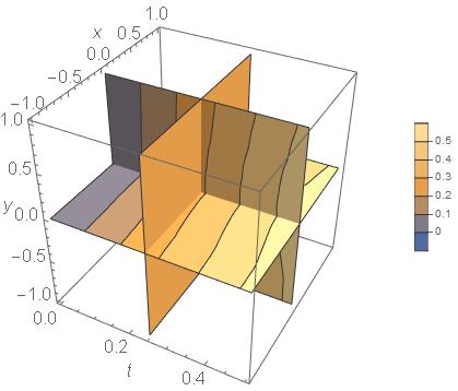
Figure 1: Numerical solution of (113) for $t\in[0,0.5]$.

From the numerical solution of (113), we see that the transition layer is located in the region $-1\leq h_{0}(x,y,t)\leq 1$ for any $x\in[-1;1],y\in[-1;1]$, and $t\in[0,0.5]$ (Fig. 1), thus Assumption 2 is satisfied.

To obtain a numerical solution of (110), the results of which will be used for the inverse problem, it is necessary to know the initial function, which we take in the form

(114) $$u_{init}(x,y,z,\mu)=\frac{u^{a}-u^{-a}}{2}\tanh\left(x+y+\frac{z-h_{0}(x,y,0)}{0.1\mu}\right)+\frac{u^{a}+u^{-a}}{2}\\ =3\tanh\left(x+y+\frac{z}{0.001}\right)-1,$$

with an inner transition layer in the vicinity of $h_{0}(x,y,0)=0$.

All the assumptions formulated in this paper are satisfied, and the considered equation (110) has a solution in the form of an autowave with a transitional moving layer localized near $h_{0}(x,y,t)$, which in the zeroth-order approximation has the form

(115) $$U_{0}=\begin{cases}\displaystyle\varphi^{(-)}(x,y,z)+\frac{\varphi^{(+)}(x,y,h_{0})-\varphi^{(-)}(x,y,h_{0})}{\exp\left(\frac{\left(h_{0}-z\right)\left(\varphi^{(+)}(x,y,h_{0})-\varphi^{(-)}(x,y,h_{0})\right)\left(1-{h_{0}}_{x}-{h_{0}}_{y}\right)}{2\mu}\right)+1},z\in[-1;h_{0}],\\ \displaystyle\varphi^{(+)}(x,y,z)+\frac{\varphi^{(-)}(x,y,h_{0})-\varphi^{(+)}(x,y,h_{0})}{\exp\left(\frac{\left(h_{0}-z\right)\left(\varphi^{(-)}(x,y,h_{0})-\varphi^{(+)}(x,y,h_{0})\right)\left(1-{h_{0}}_{x}-{h_{0}}_{y}\right)}{2\mu}\right)+1},z\in[h_{0};1].\end{cases}$$

To evaluate the accuracy of our approach, we show the asymptotic solution (115) and a high-accuracy numerical solution at time $t_{0}=0.4$ in Figures 2 and 2, respectively, from which we conclude that the asymptotic solution is highly qualified. Indeed, the error of the asymptotic solution is

$$\frac{\|U_{0}(x,y,z,t_{0})-u(x,y,z,t_{0})\|_{L^{2}([-1,1]\times[-1,1]\times[-1,1])}}{\|u(x,y,z,t_{0})\|_{L^{2}([-1,1]\times[-1,1]\times[-1,1])}}=0.0735.$$

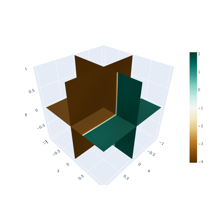
Figure 2: Asymptotic solution 2 and numerical solution 2 of PDE (110) with $t_{0}=0.4$.

5.2 Inverse problem

Now, as a more complex scenario, we consider the problem of identifying the source function $f(x,y,z)$ of problem (110) when only the noisy measurements $\{u^{\delta}_{i,j,k}\}^{p,q,v}_{i,j,k=0}$ are provided.

Because the functions $\varphi^{(-)}(x,y,z)$ and $\varphi^{(+)}(x,y,z)$ are solutions to problems (111) and (112), the asymptotic analysis allows us to reduce the original inverse problem of determining the source function $f(x,y,z)$ to a first-order equation of the asymptotic approximation of the solution of the direct problem. We use the parameters $a=1,t_{0}=0.4,\delta=5\%,p=100,q=100,v=100,v^{(-)}=58,v^{(+)}=73$.

We take the data $u(x_{i},y_{j},z_{k},t_{0})$ obtained from the numerical result (i.e., by a finite-volume method) for the forward problem [Fig. 2], which belong to the mesh knots $X_{p}=\{x_{i},0\leq i\leq p:x_{i}=x_{0}+d_{1}i,d_{1}=2a/p\}$, $Y_{q}=\{y_{j},0\leq j\leq q:y_{j}=y_{0}+d_{2}j,d_{2}=2a/q\}$, and $Z_{v}=\{z_{k},0\leq k\leq v:z_{k}=-a+d_{3}k,d_{3}=2a/v\}$. The points belonging to the transitional layer $(h_{0}(x,y,t_{0})-\Delta h/2,h_{0}(x,y,t_{0})+\Delta h/2)$ have been removed, so we use only the points with indices $i=0,\cdots,p$, $j=0,\cdots,q$ and $k=0,\cdots,v^{(-)}$, $k=v^{(+)},\cdots,v$. Artificial noise data are obtained by adding uniform noise with $\delta=5\%$ to the values $u(x_{i},y_{j},z_{k},t_{0})$ [Fig. 3]:

(116) $$u^{\delta}_{i,j,k}:=[1+\delta(2\,\text{rand}-1)]u(x_{i},y_{j},y_{k},t_{0}),$$

where “rand” returns a pseudo-random value drawn from a uniform distribution on $[0,1]$.

Following Algorithm 1, we smooth the noisy data on both regions by (63) and (64) and obtain the smooth function $u^{\varepsilon}(x,y,z,t_{0})$ [Fig. 3]. We then calculate the regularized approximate source function $f^{\delta}$ by (62) and compare it with the exact source function $f^{*}(x,y,z)=\cos{(\pi x)}\cos{(\pi y)}\cos{(\pi z)}$ (Fig. 4). The relative error of reconstructing the source function for the noise $\delta=5\%$ is

$$\frac{\|f^{\delta}-f^{*}\|_{L^{2}([-1,1]\times[-1,1]\times[-1,1])}}{\|f^{*}\|_{L^{2}([-1,1]\times[-1,1]\times[-1,1])}}=0.3674.$$

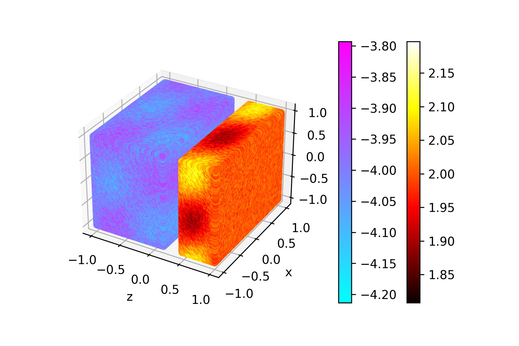
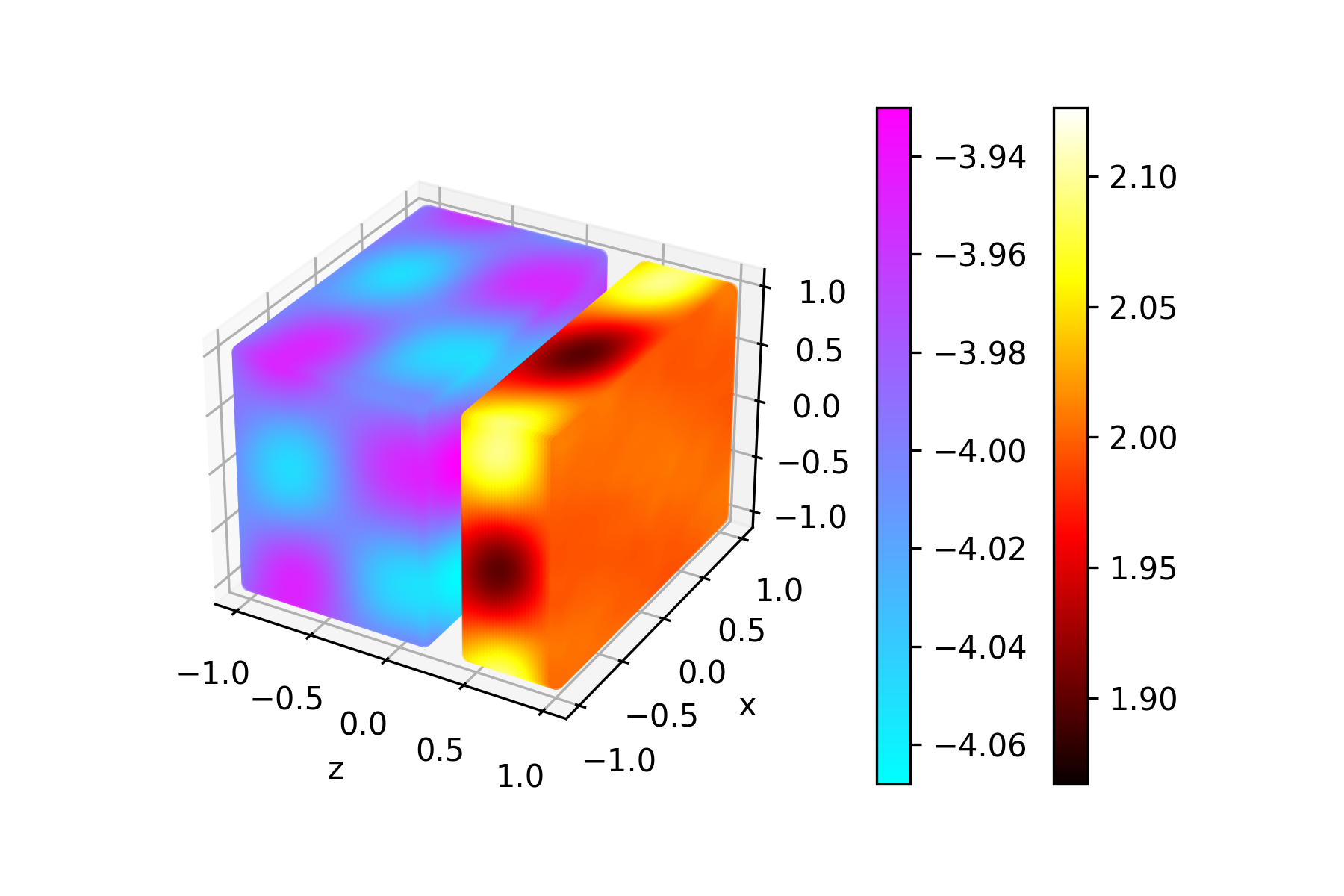
Figure 3: Noisy data $\{u^{\delta}_{i,j,k}(t_{0})\}$ with $\delta=5\%$ 3 and smooth approximate data $\{u^{\varepsilon}_{i,j,k}(t_{0})\}$ 3.

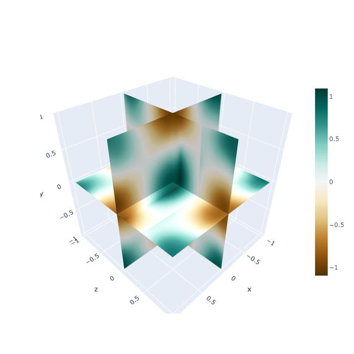
Figure 4: Reconstructed source function $f^{\delta}(x,y,z)$ 4 for $\delta=5\%$, where data in the transition layer was obtained by the linear interpolation, and exact source function $f^{*}(x)$ 4.

6 Conclusion

In this paper, by using asymptotic expansions, we developed an efficient approach for obtaining the approximate solutions of both forward and inverse problems associated with a three-dimensional nonlinear PDE of the RDA type with an internal transition layer. The merit of our approach is twofold. First, by incorporating the asymptotic method of inequalities, the existence and uniqueness of a classical solution of the PDE have been proven. Second, the procedure of asymptotic expansion can be used as one of model reduction for some inverse problems: when constructing an asymptotic solution, a equation linking measurements and unknown quantities can be explored, which produces an efficient inversion algorithm.

Note that our approach could be applied easily to many other similar problems in mathematical physics. For instance, the present model (1) can be viewed as a special case of the general model

$$\mu\Delta u-\frac{\partial u}{\partial t}=\left(\mathbf{A}\left(u,x,y,z\right),\nabla\right)u+F(u,x,y,z),$$

where $\mathbf{A}(u,x,y,z)=\left\{A_{1}(u,x,y,z),A_{2}(u,x,y,z),A_{3}(u,x,y,z)\right\}$. Having chosen the functions $A_{1}$, $A_{2}$, $A_{3}$, and $F$ so that it is possible to obtain explicit solutions for the inner and outer functions, all the results in this paper can be derived similarly.

Funding

This work was funded by the National Natural Science Foundation of China (Grant No. 12171036) and the Beijing Natural Science Foundation (Key Project No. Z210001).

References

- [1] Y. Zhang, G. Lin, P. Forssen, M. Gulliksson, T. Fornstedt, and X. Cheng. A regularization method for the reconstruction of adsorption isotherms in liquid chromatography. Inverse Problem, 32(10):105005, 2016.
- [2] G. Lin, Y. Zhang, X. Cheng, M. Gulliksson, P. Forssen, and T. Fornstedt. A regularizing Kohn-Vogelius formulation for the model-free adsorption isotherm estimation problem in chromatography. Applicable Analysis, 97:13–40, 2018.
- [3] A. Hidalgo, L. Tello, and E.F. Toro. Numerical and analytical study of an atherosclerosis in ammatory disease model. Journal of Mathematical Biology, 68:1785–1814, 2014.
- [4] C. Cosner. Reaction-diffusion-advection models for the effects and evolution of dispersal. Discrete and Continuous Dynamical Systems, 34(5):1701–1745, 2014.
- [5] A. Sogachev and O. Panferov. Modification of two-equation models to account for plant drag. Boundary-Layer Meteorology, 121:229–266, 2006.
- [6] A.V. Olchev, K. Radler, A. Sogachev, O. Panferov, and G. Gravenhorst. Application of a three-dimensional model for assessing effects of small clear-cuttings on radiation and soil temperature. Ecological Modelling, 220:3046–3056, 2009.
- [7] O. Rudenko. Inhomogeneous burgers equation with modular nonlinearity: Excitation and evolution of high-intensity waves. Doklady Mathematics, 95:291–294, 05 2017.
- [8] N. Nefedov and O. Rudenko. On front motion in a burgers-type equation with quadratic and modular nonlinearity and nonlinear amplification. Doklady Mathematics, 97:99–103, 01 2018.
- [9] N.N. Nefedov. The existence and asymptotic stability of periodic solutions with an interior layer of burgers type equations with modular advection. Mathematical Modelling of Natural Phenomena, 2019.
- [10] N. Levashova and O. Nikolaeva. The heat equation solution near the interface between two media. Model. Anal. Inform. Sist., 24:339–352, 2017.
- [11] A. Orlov, N. Levashova, and T. Burbaev. The use of asymptotic methods for modelling of the carriers wave functions in the si/sige heterostructures with quantum-confined layers. Journal of Physics: Conference Series, 586, jan 2015.
- [12] N. Levashova, A. Sidorova, A. Semina, and M. Ni. A spatio-temporal autowave model of shanghai territory development. Sustainability, 11:3658, 2019.
- [13] A. Sidorova, N. Levashova, and A.E. Semina. Autowave model of megapolis morphogenesis in the context of inhomogeneous active media. Bulletin of the Russian Academy of Sciences: Physics, 83:91–96, 2019.
- [14] N. Kopteva and M. Stynes. Stabilised approximation of interior-layer solutions of a singularly perturbed semilinear reaction–diffusion problem. Numerische Mathematik, 119:787–810, 2011.
- [15] V. Volkov, N. Nefedov, and E. Antipov. Asymptotic-numerical method for moving fronts in two-dimensional r-d-a problems. In Finite Difference Methods,Theory and Applications, pages 408–416, Cham, 2015. Springer International Publishing.
- [16] N. Kopteva and E. O’Riordan. Shishkin meshes in the numerical solution of singularly perturbed differential equations. International Journal of Numerical Analysis and Modeling, 7(3):393–415, 2010.
- [17] J. Quinn. A numerical method for a nonlinear singularly perturbed interior layer problem using an approximate layer location. Journal of Computational and Applied Mathematics, 290:500–515, 2015.
- [18] E. O’Riordan and J. Quinn. Parameter-uniform numerical methods for some linear and nonlinear singularly perturbed convection diffusion boundary turning point problems. BIT Numerical Mathematics, 51:317–337, 2011.
- [19] D. Lukyanenko, V. Volkov, and N. Nefedov. Dynamically adapted mesh construction for the efficient numerical solution of a singular perturbed reaction-diffusion-advection equation. Modeling and Analysis of Information Systems, 24:322–338, 01 2017.
- [20] D. Lukyanenko, V.B. Grigorev, V. Volkov, and M. Shishlenin. Solving of the coefficient inverse problem for a nonlinear singularly perturbed two-dimensional reaction–diffusion equation with the location of moving front data. Computers & Mathematics with Applications, 77, 11 2018.
- [21] A.N. Tikhonov, A.V. Goncharsky, V.V. Stepanov, and A.G. Yagola. Numerical Methods for the Solution of Ill-Posed Problems. Kluwer Academic Publishers, Dordrecht, 1995.
- [22] V. Isakov. Inverse Source Problems. American Mathematical Society, New York, 1990.
- [23] D. Lukyanenko, M. Shishlenin, and V. Volkov. Solving of the coefficient inverse problems for a nonlinear singularly perturbed reaction-diffusion-advection equation with the final time data. Commun. Nonlinear Sci. Numer. Simul., 54:233–247, 2018.
- [24] D. Chaikovskii and Y. Zhang. Convergence analysis for forward and inverse problems in singularly perturbed time-dependent reaction-advection-diffusion equations. Journal of Computational Physics, 470:111609, 2022.
- [25] E.A. Antipov, N.T. Levashova, and N.N. Nefedov. Asymptotic approximation of the solution of the reaction-diffusion-advection equation with a nonlinear advective term. Modelirovanie i Analiz Informatsionnykh Sistem, 25:18–32, 01 2018.
- [26] A.B. Vasil’eva and V.F. Butuzov. Asimptoticheskie metody v teorii singuljarnyh vozmushhenij (in Russian). Vysshaja shkola, Moskva, 1990.
- [27] A.B. Vasil’eva, V. Butuzov, and N. Nefedov. Contrast structures in singularly perturbed problems. Fundamental and Applied Mathematics, 4(3):799–851, 1998.
- [28] V. Butuzov, A. B. Vasil’eva, and N. Nefedov. Asymptotic theory of contrast structures. Automation and Remote Control, 58:1068–1091, 1997.
- [29] Hanke M. and O. Scherzer. Inverse problems light: Numerical differentiation. The American Mathematical Monthly, 108(6):512–521, 2001.
- [30] Y.B. Wang and T. Wei. Numerical differentiation for two-dimensional scattered data. Journal of Mathematical Analysis and Applications, 312(1):121–137, 2005.
- [31] N.N. Nefedov. The method of differential inequalities for some classes of nonlinear singularly perturbed problems with internal layers. Differential Equations, 31:1142–1149, 1995.
- [32] D.H. Sattinger. Monotone methods in elliptic and parabolic boundary value problems. Indiana University Mathematics Journal, 21:979–1001, 1972.
- [33] N.N. Nefedov, L. Recke, and K.R. Schneider. Existence and asymptotic stability of periodic solutions with an interior layer of reaction–advection–diffusion equations. Journal of Mathematical Analysis and Applications, 405(1):90–103, 2013.
- [34] E.A. Antipov, N.T. Levashova, and N.N. Nefedov. Asymptotics of the front motion in the reaction-diffusion-advection problem. Computational Mathematics and Mathematical Physics, 54:1536–1549, 2014.
- [35] C.V. Pao. Nonlinear Parabolic and Elliptic Equations. Plenum Press, New York, 1992.