Abstract

Recently, graph (network) data is an emerging research area in artificial intelligence, machine learning and statistics. In this work, we are interested in whether node’s labels (people’s responses) are affected by their neighbor’s features (friends’ characteristics). We propose a novel latent logistic regression model to describe the network dependence with binary responses. The key advantage of our proposed model is that a latent binary indicator is introduced to indicate whether a node is susceptible to the influence of its neighbour. A score-type test is proposed to diagnose the existence of network dependence. In addition, an EM-type algorithm is used to estimate the model parameters under network dependence. Extensive simulations are conducted to evaluate the performance of our method. Two public datasets are used to illustrate the effectiveness of the proposed latent logistic regression model.

Keywords: Artificial intelligence; EM algorithm; Graph data; Logistic regression; ROC curves; Social network

1 Introduction

Nowadays, graphs or networks are widely used in many research fields, such as social interactions, protein-protein interactions, chemical molecule bonds, transport networks, etc. Great efforts have been focused on network data in the literature. For example, Zhu et al. (2017) proposed a network vector autoregressive model. Yan et al. (2019) studied the maximum likelihood estimation of a directed network model with covariates. Zhang et al. (2022) studied some topics on large scale social networks. Chandna et al. (2021) considered the local linear estimation of the graphon function. Zhu et al. (2021) introduced a network functional varying coefficient model. Pan et al. (2022) proposed a latent space logistic regression model for link prediction with social networks. Zhao et al. (2022) proposed a dimension reduction method for covariates in network data, etc.

The logistic regression is a very famous statistical tool, which plays an important role in practical applications. e.g. finance research Li et al. (2019), public health Lemon et al. (2003), medicine Lu and Yang (2012), education Pyke and Sheridan (1993), bioinformatics Wu et al. (2009). There have been some methodological developments on the logistic regression. e.g. Landwehr et al. (1984) proposed a graphical methods for assessing logistic regression models. Stefanski and Carroll (1985) studied the logistic regression model when covariates are subject to measurement error. Jennings (1986) investigated the outliers and residual distributions in logistic regression. Efron (1988) used the logistic regression techniques to estimate hazard rates and survival curves from censored data. Carroll and Pederson (1993) investigated robustness in the logistic regression model. Meier et al. (2008) extended the group lasso to logistic regression models. Liu et al. (2009) proposed an algorithm for solving large-scale sparse logistic regression. Singh et al. (2009) examined the problem of efficient feature selection for logistic regression on very large data sets. Shi et al. (2010) and Yuan et al. (2012) studied some algorithms for L1-regularized logistic regression. Conroy and Sajda (2012) proposed a fast and exact model selection procedure for L2-regularized logistic regression. Das et al. (2013) introduced new supervised and semi-supervised learning algorithms based on locally-weighted logistic regression. Tripathi et al. (2017) considered estimation of the probability density function and the cumulative distribution function of the generalized logistic distribution. Schein and Ungar (2007) and Yang and Loog (2018) studied the active learning methods for logistic regression. Wang (2020) studied binary logistic regression for rare events data. Han et al. (2019) presented an efficient algorithm for logistic regression on homomorphic encrypted data. Wang et al. (2018) and Zuo et al. (2021) considered the optimal subsmapling for logistic regression in big data, among others.

However, the above-mentioned logistic regression methods did not consider the effects of networks. For example, does a persion like to playing a game given that his/her friends like it? Will the customers by a commodity if their friends have bought it? In this work, we are interested in exploring whether certain type of network dependence exists with binary outcomes data and to quantify this dependence structure if it exists. To deal with this issue, we propose a logistic model with latent binary indicator, which has the ability to describe whether a node is susceptible to the influence of its neighbor. Our method has the following two advantages: First, the proposed logistic model with a latent binary indicator is very flexibility in practical applications. It provides a solution to estimate the probability that a node might be affected by neighbor’s characteristics in the network. Hence, we can detect a subgroup of nodes who are more likely to be influenced by their neighbors. Second, we give a score-type test for detecting the existence of the network dependence in the logistic model. An EM algorithm is employed to estimate the model parameters, which leads to consistence estimator with desirable performance in simulations.

The remainder of this article is organized as follows: In Section 2, we introduce a latent logistic regression model. In Section 3, we propose a supremum score test statistic to detect the existence of network dependence. In Section 4, an EM-type estimation algorithm is proposed. Simulations and a real data application are presented in Sections 5 and 6, respectively. In Section 7, we give some concluding remarks.

2 Model and Notation

Let $G=(V,E)$ be an undirected graph with nodes $V$ and edges $E$. Assume that there are $n$ nodes belonging to two classes. Let $Y_{i}\in\{0,1\}$ and $\mathbf{X}_{i}=(X_{i1},\cdots,X_{ip})^{\prime}\in\mathbb{R}^{p}$ be the binary label and feature vector of the $i$-th node $v_{i}$, $i=1,\cdots,n$. Given the graph structure of $G$, we propose a novel latent logistic regression model:

$${\mathbb{P}}(Y_{i}=1|\mathbf{X}_{i},\zeta_{i}) =\frac{\exp\{\beta_{0}+\mathbf{X}_{i}^{\prime}{\bm{\beta}}+\delta\zeta_{i}\sum_{j=1}^{n}a_{ij}\mathbf{X}_{j}^{\prime}{\bm{\beta}}\}}{1+\exp\{\beta_{0}+\mathbf{X}_{i}^{\prime}{\bm{\beta}}+\delta\zeta_{i}\sum_{j=1}^{n}a_{ij}\mathbf{X}_{j}^{\prime}{\bm{\beta}}\}},~{}~{}i=1,\cdots,n,$$ (2.1)

where $\beta_{0}\in\mathbb{R}$ is an intercept, ${\bm{\beta}}=(\beta_{1},\cdots,\beta_{p})^{\prime}$ is the vector of regression parameters, $\mathbf{A}=(a_{ij})$ is the adjacency matrix ($a_{ii}=0$, and $a_{ij}=1$ if there is an edge between the $i$th node and $j$th node, $a_{ij}=0$ otherwise); $\zeta_{i}\in\{0,1\}$ is a latent indicator denoting whether the label (response) of $i$th node depends on its neighbor’s features. Note that $\zeta_{i}$ is unobservable, and we assume that

$${\mathbb{P}}(\zeta_{i}=1|\mathbf{X}_{i})=\frac{\exp\{\gamma_{0}+\mathbf{X}_{i}^{\prime}{\bm{\gamma}}\}}{1+\exp\{\gamma_{0}+\mathbf{X}_{i}^{\prime}{\bm{\gamma}}\}}.$$ (2.2)

The parameter $\delta$ plays the role of describing the magnitude of the dependence of a node to its neighbor. When $\delta=0$, there is no network dependence between labels of connected nodes, and the parameters $\gamma_{0}$ and ${\bm{\gamma}}$ are not estimable in this case. In what follows, we will proposed a method to test the null hypothesis $H_{0}:\delta=0$, and then give an EM-type algorithm to estimate the model parameters under $\delta\neq 0$.

3 Test for $H_{0}:\delta=0$

First we assume that $\bm{\zeta}=(\zeta_{1},\cdots,\zeta_{n})^{\prime}$ is known. The log likelihood function is

$$L({\bm{\theta}};{\bm{\zeta}}) = \sum_{i=1}^{n}\Bigg{[}Y_{i}\Big{(}\beta_{0}+\mathbf{X}_{i}^{\prime}{\bm{\beta}}+\delta\zeta_{i}\sum_{j=1}^{n}a_{ij}\mathbf{X}_{j}^{\prime}{\bm{\beta}}\Big{)}$$ (3.1)

$$-\log\bigg{(}1+\exp\Big{\{}\beta_{0}+\mathbf{X}_{i}^{\prime}{\bm{\beta}}+\delta\zeta_{i}\sum_{j=1}^{n}a_{ij}\mathbf{X}_{j}^{\prime}{\bm{\beta}}\Big{\}}\bigg{)}\Bigg{]},$$

where ${\bm{\theta}}=(\delta,\beta_{0},{\bm{\beta}}^{\prime})^{\prime}$. Under $H_{0}$, model (2.1) reduces to the standard logistic model. Let $\tilde{\beta}_{0}$ and $\tilde{{\bm{\beta}}}$ denote the maximum likelihood estimator under the null. Denote $\tilde{{\bm{\theta}}}=(0,\tilde{\beta}_{0},\tilde{{\bm{\beta}}}^{\prime})^{\prime}$. Some calculations lead to the following score function:

$$S(\tilde{{\bm{\theta}}};{\bm{\zeta}})=\frac{\partial L({\bm{\theta}};{\bm{\zeta}})}{\partial\delta}|_{{\bm{\theta}}=\tilde{{\bm{\theta}}}}=\sum_{i=1}^{n}\tilde{Z}_{i}\left[Y_{i}-\frac{\exp(\tilde{\beta}_{0}+\mathbf{X}_{i}^{\prime}\tilde{{\bm{\beta}}})}{1+\exp(\tilde{\beta}_{0}+\mathbf{X}_{i}^{\prime}\tilde{{\bm{\beta}}})}\right],$$ (3.2)

where $\tilde{Z}_{i}=\zeta_{i}\sum_{j=1}^{n}a_{ij}\mathbf{X}_{j}^{\prime}\tilde{{\bm{\beta}}}$. Because ${\bm{\zeta}}$ is not available in $\tilde{Z}_{i}$’s, we propose to replace $\zeta_{i}$ with its expectation $E(\zeta_{i})=P(\zeta_{i}=1|\mathbf{X}_{i})$ given in (2.2). For convenience, denote $\tilde{Z}_{i}^{*}=E(\zeta_{i})\sum_{j=1}^{n}a_{ij}\mathbf{X}_{j}^{\prime}\tilde{{\bm{\beta}}}$. After replacing $\tilde{Z}_{i}$ with $\tilde{Z}_{i}^{*}$ in (3.2), we obtain a score-type statistic:

$$S^{*}(\tilde{{\bm{\theta}}};{\bm{\phi}})=\sum_{i=1}^{n}\tilde{Z}^{*}_{i}\left[Y_{i}-\frac{\exp(\tilde{\beta}_{0}+\mathbf{X}_{i}^{\prime}\tilde{{\bm{\beta}}})}{1+\exp(\tilde{\beta}_{0}+\mathbf{X}_{i}^{\prime}\tilde{{\bm{\beta}}})}\right],$$ (3.3)

where ${\bm{\phi}}=(\gamma_{0},{\bm{\gamma}}^{\prime})^{\prime}$.

Motivated by Fan et al. (2017), we propose a supremum score test statistic:

$$T_{n}=\sup\limits_{{\bm{\phi}}\in{\bm{\Gamma}}}\frac{\{S^{*}(\tilde{{\bm{\theta}}};{\bm{\phi}})\}^{2}}{\sum_{i=1}^{n}\{U_{i}^{*}(\tilde{{\bm{\theta}}};{\bm{\phi}})\}^{2}},$$ (3.4)

where ${\bm{\Gamma}}\in\mathbb{R}^{p+1}$, and

$$U_{i}^{*}(\tilde{{\bm{\theta}}};{\bm{\phi}}) = \left[Y_{i}-\frac{\exp(\tilde{\beta}_{0}+\mathbf{X}_{i}^{\prime}\tilde{{\bm{\beta}}})}{1+\exp(\tilde{\beta}_{0}+\mathbf{X}_{i}^{\prime}\tilde{{\bm{\beta}}})}\right]\left\{\tilde{Z}^{*}_{i}-\mathcal{B}_{n}^{*}(\tilde{{\bm{\theta}}})\mathcal{I}_{n}^{-1}(\tilde{{\bm{\theta}}})(1,\mathbf{X}_{i}^{\prime})^{\prime}\right\},$$

where $\mathcal{I}_{n}(\tilde{{\bm{\theta}}})=-\frac{\partial^{2}L({\bm{\theta}};{\bm{\zeta}})}{\partial{\bm{\eta}}{\bm{\eta}}^{\prime}}|_{{\bm{\theta}}=\tilde{{\bm{\theta}}}}$, $\mathcal{B}_{n}(\tilde{{\bm{\theta}}})=-\frac{\partial^{2}L({\bm{\theta}};{\bm{\zeta}})}{\partial\delta\partial{\bm{\eta}}^{\prime}}|_{{\bm{\theta}}=\tilde{{\bm{\theta}}}}$, ${\bm{\eta}}=(\beta_{0},{\bm{\beta}}^{\prime})^{\prime}$ and $\mathcal{B}^{*}_{n}(\tilde{{\bm{\theta}}})$ is given from $\mathcal{B}_{n}(\tilde{{\bm{\theta}}})$ by replacing $\zeta_{i}$ with its expectation $E(\zeta_{i})=P(\zeta_{i}=1|\mathbf{X}_{i})$. To be more specific, we have the following two explicit expressions:

$$\mathcal{I}_{n}(\tilde{{\bm{\theta}}})=\sum_{i=1}^{n}\left[\frac{\exp(\tilde{\mathbf{X}}^{\prime}_{i}\tilde{{\bm{\eta}}})}{1+\exp(\tilde{\mathbf{X}}^{\prime}_{i}\tilde{{\bm{\eta}}})}-\left\{\frac{\exp(\tilde{\mathbf{X}}^{\prime}_{i}\tilde{{\bm{\eta}}})}{1+\exp(\tilde{\mathbf{X}}^{\prime}_{i}\tilde{{\bm{\eta}}})}\right\}^{2}\right]\tilde{\mathbf{X}}_{i}\tilde{\mathbf{X}}^{\prime}_{i},$$

and

$$\mathcal{B}_{n}(\tilde{{\bm{\theta}}}) = -\sum_{i=1}^{n}\Bigg{[}\zeta_{i}\bigg{\{}Y_{i}-\frac{\exp(\tilde{\mathbf{X}}^{\prime}_{i}\tilde{{\bm{\eta}}})}{1+\exp(\tilde{\mathbf{X}}^{\prime}_{i}\tilde{{\bm{\eta}}})}\bigg{\}}\Big{(}0,\sum_{j=1}^{n}a_{ij}\mathbf{X}_{j}^{\prime}\Big{)}$$

$$+\zeta_{i}\sum_{j=1}^{n}a_{ij}\mathbf{X}_{j}^{\prime}\tilde{{\bm{\beta}}}\bigg{(}\bigg{\{}\frac{\exp(\tilde{\mathbf{X}}^{\prime}_{i}\tilde{{\bm{\eta}}})}{1+\exp(\tilde{\mathbf{X}}^{\prime}_{i}\tilde{{\bm{\eta}}})}\bigg{\}}^{2}-\frac{\exp(\tilde{\mathbf{X}}^{\prime}_{i}\tilde{{\bm{\eta}}})}{1+\exp(\tilde{\mathbf{X}}^{\prime}_{i}\tilde{{\bm{\eta}}})}\bigg{)}\mathbf{\tilde{X}}_{i}^{\prime}\Bigg{]},$$

where $\tilde{{\bm{\eta}}}=(\tilde{\beta}_{0},\tilde{{\bm{\beta}}}^{\prime})^{\prime}$, and $\tilde{\mathbf{X}}_{i}=(1,\mathbf{X}_{i}^{\prime})^{\prime}$.

Theorem 1

As $n\rightarrow\infty$, we have $T_{n}$ converges in distribution to $\sup\limits_{{\bm{\phi}}\in{\bm{\Gamma}}}G^{2}({\bm{\phi}})$ under $H_{0}$, where $\{G({\bm{\phi}}):{\bm{\phi}}\in{\bm{\Gamma}}\}$ is a mean zero Gaussian process with the covariance function

$${\bm{\Sigma}}({\bm{\phi}}_{1},{\bm{\phi}}_{2})=\lim_{n\rightarrow\infty}\frac{\sum_{i=1}^{n}U_{i}^{*}({\bm{\theta}}_{t};{\bm{\phi}}_{1})U_{i}^{*}({\bm{\theta}}_{t};{\bm{\phi}}_{2})}{[\sum_{i=1}^{n}\{U_{i}^{*}({\bm{\theta}}_{t};{\bm{\phi}}_{1})\}^{2}\sum_{i=1}^{n}\{U_{i}^{*}({\bm{\theta}}_{t};{\bm{\phi}}_{2})\}^{2}]^{1/2}},$$

for any ${\bm{\phi}}_{1}$, ${\bm{\phi}}_{2}\in{\bm{\Gamma}}$.

We adopt a resampling method in order to obtain the the critical value of the asymptotic distribution of $T_{n}$ under $H_{0}$. To be more specific, we define a perturbed test statistic:

$$T_{n}^{*}=\sup\limits_{{\bm{\phi}}\in{\bm{\Gamma}}}\frac{\{\sum_{i=1}^{n}\xi_{i}U_{i}^{*}(\tilde{{\bm{\theta}}};{\bm{\phi}})\}^{2}}{\sum_{i=1}^{n}\{U_{i}^{*}(\tilde{{\bm{\theta}}};{\bm{\phi}})\}^{2}},$$ (3.5)

where $\xi_{1},\cdots,\xi_{n}$ are independently generated from $N(0,1)$. Note that $T_{n}$ and $T_{n}^{*}$ own the same asymptotic distribution under $H_{0}$. By repeatedly generating a great deal of perturbed statistics, we can obtain the empirical upper $\alpha$-quantile, $C_{\alpha}$, of the perturbed statistics $T_{n}^{*}$’s. The null $H_{0}$ is rejected if $T_{n}>C_{\alpha}$.

4 Estimation Method

In this section, we assume $\delta\neq 0$. Therefore, the models (2.1) and (2.2) are identifiable in terms of parameter ${\bm{\Theta}}=(\delta,\beta_{0},{\bm{\beta}}^{\prime},{\bm{\phi}}^{\prime})^{\prime}$. The complete log likelihood function is

$$L({\bm{\Theta}}) = \sum_{i=1}^{n}\Bigg{[}Y_{i}\Big{(}\beta_{0}+\mathbf{X}_{i}^{\prime}{\bm{\beta}}+\delta\zeta_{i}\sum_{j=1}^{n}a_{ij}\mathbf{X}_{j}^{\prime}{\bm{\beta}}\Big{)}-\log\bigg{(}1+\exp\Big{\{}\beta_{0}+\mathbf{X}_{i}^{\prime}{\bm{\beta}}+\delta\zeta_{i}\sum_{j=1}^{n}a_{ij}\mathbf{X}_{j}^{\prime}{\bm{\beta}}\Big{\}}\bigg{)}$$ (4.1)

$$+~{}\zeta_{i}(\gamma_{0}+\mathbf{X}_{i}^{\prime}{\bm{\gamma}})-\log\big{(}1+\exp\{\gamma_{0}+\mathbf{X}_{i}^{\prime}{\bm{\gamma}}\}\big{)}\Bigg{]}.$$

To estimate the parameter of interest ${\bm{\Theta}}$, we adopt an EM-type algorithm towards the log likelihood function given in (4.1): Let $\mathcal{D}_{n}=\{(\mathbf{X}_{i},Y_{i})\}_{i=1}^{n}$ denote the observed data, and $\hat{{\bm{\Theta}}}^{(k)}$ be the estimate of ${\bm{\Theta}}$ at the $k$th iteration. In the E-step of $(k+1)$th iteration, we calculate the conditional expectation of $L({\bm{\Theta}})$ given the observed data $\mathcal{D}_{n}$ and $\hat{{\bm{\Theta}}}^{(k)}$. i.e.,

$$\ell\big{(}{\bm{\Theta}}|\hat{{\bm{\Theta}}}^{(k)}\big{)} = E\big{\{}L({\bm{\Theta}})|\mathcal{D}_{n},\hat{{\bm{\Theta}}}^{(k)}\big{\}}$$ (4.2)

$$= \underbrace{\sum_{i=1}^{n}Y_{i}\bigg{[}\beta_{0}+\mathbf{X}_{i}^{\prime}{\bm{\beta}}+\hat{w}_{ik}\delta\sum_{j=1}^{n}a_{ij}\mathbf{X}_{j}^{\prime}{\bm{\beta}}\bigg{]}}_{\ell_{1}({\bm{\Theta}}|\hat{{\bm{\Theta}}}^{(k)})}+\ell_{2}\big{(}{\bm{\Theta}}|\hat{{\bm{\Theta}}}^{(k)}\big{)}+\ell_{3}\big{(}{\bm{\Theta}}|\hat{{\bm{\Theta}}}^{(k)}\big{)},$$

where $\hat{w}_{ik}=E\{\zeta_{i}|\mathcal{D}_{n},\hat{{\bm{\Theta}}}^{(k)}\}={T_{i1}^{(k)}}/\{T_{i1}^{(k)}+T_{i2}^{(k)}\}$ with

$$T_{i1}^{(k)} = \frac{\exp\bigg{\{}Y_{i}\Big{(}\hat{\beta}^{(k)}_{0}+\mathbf{X}_{i}^{\prime}\hat{{\bm{\beta}}}^{(k)}+\hat{\delta}^{(k)}\sum_{j=1}^{n}a_{ij}\mathbf{X}_{j}^{\prime}\hat{{\bm{\beta}}}^{(k)}\Big{)}\bigg{\}}}{1+\exp\Big{\{}\hat{\beta}^{(k)}_{0}+\mathbf{X}_{i}^{\prime}\hat{{\bm{\beta}}}^{(k)}+\hat{\delta}^{(k)}\sum_{j=1}^{n}a_{ij}\mathbf{X}_{j}^{\prime}\hat{{\bm{\beta}}}^{(k)}\Big{\}}}\hat{P}_{i}^{(k)},$$

$$T_{i2}^{(k)} = \frac{\exp\bigg{\{}Y_{i}\Big{(}\hat{\beta}^{(k)}_{0}+\mathbf{X}_{i}^{\prime}\hat{{\bm{\beta}}}^{(k)}\Big{)}\bigg{\}}}{1+\exp\Big{\{}\hat{\beta}^{(k)}_{0}+\mathbf{X}_{i}^{\prime}\hat{{\bm{\beta}}}^{(k)}\Big{\}}}(1-\hat{P}_{i}^{(k)}),$$

$$\hat{P}_{i}^{(k)} = \frac{\exp\Big{\{}\hat{\gamma}^{(k)}_{0}+\mathbf{X}_{i}^{\prime}\hat{{\bm{\gamma}}}^{(k)}\Big{\}}}{1+\exp\Big{\{}\hat{\gamma}^{(k)}_{0}+\mathbf{X}_{i}^{\prime}\hat{{\bm{\gamma}}}^{(k)}\Big{\}}},$$

and

$$\ell_{2}\big{(}{\bm{\Theta}}|\hat{{\bm{\Theta}}}^{(k)}\big{)} = -\sum_{i=1}^{n}\hat{w}_{ik}\log\bigg{(}1+\exp\Big{\{}\beta_{0}+\mathbf{X}_{i}^{\prime}{\bm{\beta}}+\delta\sum_{j=1}^{n}a_{ij}\mathbf{X}_{j}^{\prime}{\bm{\beta}}\Big{\}}\bigg{)}$$

$$-\sum_{i=1}^{n}(1-\hat{w}_{ik})\log\big{(}1+\exp\{\beta_{0}+\mathbf{X}_{i}^{\prime}{\bm{\beta}}\}\big{)}$$

$$\ell_{3}\big{(}{\bm{\Theta}}|\hat{{\bm{\Theta}}}^{(k)}\big{)} = \sum_{i=1}^{n}\Big{[}\hat{w}_{ik}(\gamma_{0}+\mathbf{X}_{i}^{\prime}{\bm{\gamma}})-\log\big{(}1+\exp\{\gamma_{0}+\mathbf{X}_{i}^{\prime}{\bm{\gamma}}\}\big{)}\Big{]}.$$

In the M-step of $(k+1)$-th iteration, we can separately maximize the functions $\ell_{1}\big{(}{\bm{\Theta}}|\hat{{\bm{\Theta}}}^{(k)}\big{)}+\ell_{2}\big{(}{\bm{\Theta}}|\hat{{\bm{\Theta}}}^{(k)}\big{)}$ and $\ell_{3}\big{(}{\bm{\Theta}}|\hat{{\bm{\Theta}}}^{(k)}\big{)}$. Because $\ell_{3}\big{(}{\bm{\Theta}}|\hat{{\bm{\Theta}}}^{(k)}\big{)}$ only contains parameters $\gamma_{0}$ and ${\bm{\gamma}}$, it is straight-forward to find the numerical maximizer $\hat{{\bm{\phi}}}^{(k+1)}=(\hat{\gamma}^{(k+1)}_{0},\hat{{\bm{\gamma}}}^{(k+1)\prime})^{\prime}$ via Newton-Raphson algorithm. To maximize $\ell_{1}\big{(}\cdot|\hat{{\bm{\Theta}}}^{(k)}\big{)}+\ell_{2}\big{(}\cdot|\hat{{\bm{\Theta}}}^{(k)}\big{)}$ with respect to $\delta$, $\beta_{0}$ and ${\bm{\beta}}$, we suggest to use an iterative optimization procedure. Given $\beta_{0}$ and ${\bm{\beta}}$, the function $\ell_{1}\big{(}\cdot|\hat{{\bm{\Theta}}}^{(k)}\big{)}+\ell_{2}\big{(}\cdot|\hat{{\bm{\Theta}}}^{(k)}\big{)}$ a univariate concave function of $\delta$, which can be easily maximized by Newton-Raphson method. Denote

$$\hat{\delta}^{(k+1)}=\arg\max_{\delta}\Big{\{}\ell_{1}\big{(}\delta,\hat{\beta}_{0}^{(k)},\hat{{\bm{\beta}}}^{(k)}|\hat{{\bm{\Theta}}}^{(k)}\big{)}+\ell_{2}\big{(}\delta,\hat{\beta}_{0}^{(k)},\hat{{\bm{\beta}}}^{(k)}|\hat{{\bm{\Theta}}}^{(k)}\big{)}\Big{\}}.$$

In order to guarantee algorithmic stability, we specify $\delta=\hat{\delta}^{(k+1)}$ and ${\bm{\beta}}=\hat{{\bm{\beta}}}^{(k)}$ in the term $\delta\sum_{j=1}^{n}a_{ij}\mathbf{X}_{j}^{\prime}{\bm{\beta}}$ of $\ell_{1}\big{(}\cdot|\hat{{\bm{\Theta}}}^{(k)}\big{)}+\ell_{2}\big{(}\cdot|\hat{{\bm{\Theta}}}^{(k)}\big{)}$, which leads to profiled log likelihood function of $\beta_{0}$ and ${\bm{\beta}}$:

$$L_{pro}(\beta_{0},{\bm{\beta}}) = \sum_{i=1}^{n}Y_{i}(\beta_{0}+\mathbf{X}_{i}^{\prime}{\bm{\beta}}+\hat{w}_{ik}\hat{u}_{ik})-\sum_{i=1}^{n}\hat{w}_{ik}\log\bigg{(}1+\exp\Big{\{}\beta_{0}+\mathbf{X}_{i}^{\prime}{\bm{\beta}}+\hat{u}_{ik}\Big{\}}\bigg{)}$$

$$-\sum_{i=1}^{n}(1-\hat{w}_{ik})\log\big{(}1+\exp\{\beta_{0}+\mathbf{X}_{i}^{\prime}{\bm{\beta}}\}\big{)},$$

where $\hat{u}_{ik}=\hat{\delta}^{(k+1)}\sum_{j=1}^{n}a_{ij}\mathbf{X}_{j}^{\prime}\hat{{\bm{\beta}}}^{(k)}$. Denote $(\hat{\beta}_{0}^{(k+1)},\hat{{\bm{\beta}}}^{(k+1)})$ as the maximizer of $L_{pro}(\beta_{0},{\bm{\beta}})$. In the proposed EM algorithm, we set the initial estimators of the parameters as follows: $\hat{\delta}^{(0)}=0$, $\hat{\gamma}_{0}^{(0)}=0$, $\hat{{\bm{\gamma}}}^{(0)}=\mathbf{0}$, $\hat{\beta}_{0}^{(0)}$ and $\hat{{\bm{\beta}}}^{(0)}$ are the maximum likelihood estimators of classical logistic regression. We repeatedly apply the E-step and M-step until convergence with $\|\hat{{\bm{\Theta}}}^{(k+1)}-\hat{{\bm{\Theta}}}^{(k)}\|<10^{-6}$. The final estimator is denoted as $\hat{{\bm{\Theta}}}=(\hat{\delta},\hat{\beta}_{0},\hat{{\bm{\beta}}}^{\prime},\hat{\gamma}_{0},\hat{{\bm{\gamma}}}^{\prime})^{\prime}$. The performance of EM-based estimator will be carefully studied via numerical simulation. Here we point out that the term $\hat{w}_{ik}$ at convergence indicates the posterior probability that the $i$th node might be affected by its neighbor’s behavior. For $i=1,\cdots,n$, we denote $\hat{w}_{i}={T_{i1}}/\{T_{i1}+T_{i2}\}$, where

$$T_{i1} = \frac{\exp\bigg{\{}Y_{i}\Big{(}\hat{\beta}_{0}+\mathbf{X}_{i}^{\prime}\hat{{\bm{\beta}}}+\hat{\delta}\sum_{j=1}^{n}a_{ij}\mathbf{X}_{j}^{\prime}\hat{{\bm{\beta}}}\Big{)}\bigg{\}}}{1+\exp\Big{\{}\hat{\beta}_{0}+\mathbf{X}_{i}^{\prime}\hat{{\bm{\beta}}}+\hat{\delta}\sum_{j=1}^{n}a_{ij}\mathbf{X}_{j}^{\prime}\hat{{\bm{\beta}}}\Big{\}}}\hat{P}_{i},$$

$$T_{i2} = \frac{\exp\bigg{\{}Y_{i}\Big{(}\hat{\beta}_{0}+\mathbf{X}_{i}^{\prime}\hat{{\bm{\beta}}}\Big{)}\bigg{\}}}{1+\exp\Big{\{}\hat{\beta}_{0}+\mathbf{X}_{i}^{\prime}\hat{{\bm{\beta}}}\Big{\}}}(1-\hat{P}_{i}),$$

$$\hat{P}_{i} = \frac{\exp\Big{\{}\hat{\gamma}_{0}+\mathbf{X}_{i}^{\prime}\hat{{\bm{\gamma}}}\Big{\}}}{1+\exp\Big{\{}\hat{\gamma}_{0}+\mathbf{X}_{i}^{\prime}\hat{{\bm{\gamma}}}\Big{\}}}.$$

We call $\hat{w}_{i}$ as the posterior “susceptible” probability for the $i$th node. A larger $\hat{w}_{i}$ indicates that the outcome of $i$th node is more likely to be by its neighbor’s feature. In this case, the predicted outcome $\hat{Y}_{i}$ satisfies:

$$\mathbb{{P}}(\hat{Y}_{i}=1|\mathbf{X}_{i},\hat{\zeta}_{i}) =\frac{\exp\{\hat{\beta}_{0}+\mathbf{X}_{i}^{\prime}\hat{{\bm{\beta}}}+\hat{\delta}\hat{\zeta}_{i}\sum_{j=1}^{n}a_{ij}\mathbf{X}_{j}^{\prime}\hat{{\bm{\beta}}}\}}{1+\exp\{\hat{\beta}_{0}+\mathbf{X}_{i}^{\prime}\hat{{\bm{\beta}}}+\hat{\delta}\hat{\zeta}_{i}\sum_{j=1}^{n}a_{ij}\mathbf{X}_{j}^{\prime}\hat{{\bm{\beta}}}\}},~{}~{}i=1,\cdots,n,$$ (4.3)

where $\hat{\delta}$, $\hat{\beta}_{0}$ and $\hat{{\bm{\beta}}}$ are the EM-based estimator; $\hat{\zeta}_{i}$ is generated from the Binomial distribution with $\mathbb{P}(\hat{\zeta}_{i}=1)=\hat{w}_{i}$, $i=1,\cdots,n$.

Table 1. Type I error and power of the proposed test with significance level $\alpha=0.05$^†.  

		$\delta=0$		$\delta=0.01$		$\delta=0.03$		$\delta=0.05$		$\delta=0.10$
Case I		0.048		0.116		0.802		0.996		1
Case II		0.048		0.098		0.794		0.992		1

 

5 Simulation Study

In this section, we conduct some simulations to verify the performance of our proposed method. We generate the graph (network) from the stochastic block model Holland et al. (1983). Specifically, we assume there are five communities in the network, and the stochastic block model is given by

$$\mathbb{P}(a_{ij}=1)=1-\mathbb{P}(a_{ij}=0)=\mathbf{P}_{C_{i}C_{j}},$$

where $\mathbf{P}$ is a $5\times 5$ symmetric matrix whose $(C_{i},C_{j})$th element $\mathbf{P}_{C_{i}C_{j}}$ denotes the probability that communities $C_{i}$ and $C_{j}$ are connected. The total number of nodes is set as $n=2000$, and the numbers of nodes contained in each community are $(500,500,400,400,200)$. The probability matrix $\mathbf{P}$ has elements $\mathbf{P}_{11}=0.01$, $\mathbf{P}_{22}=\mathbf{P}_{55}=0.10$, $\mathbf{P}_{33}=0.05$, $\mathbf{P}_{44}=0.15$, and $\mathbf{P}_{C_{i}C_{j}}=10^{-4}$ for $C_{i}\neq C_{j}$. The covariates $\mathbf{X}_{i}=(X_{i1},X_{i2})^{\prime}$ are generated from two situations:

Case I: $X_{i1}$ follows from a Bernoulli distribution with the success probability 0.5, and $X_{i2}$ follows from a uniform distribution over $(-1,1)$.

Case II: $X_{i1}$ follows from $N(0,1)$ and $X_{i2}$ follows from $N(0,2)$.
We set the parameters $\beta_{0}=0.5$, $\beta_{1}=-1$, $\beta_{2}=1$, $\gamma_{0}=0$, $\gamma_{1}=-1$ and $\gamma_{2}=1$. The computation is implemented with the help of R software. All the simulation results are based on 500 replicates.

Table 2. The Bias and MSE of estimators with proposed method^†.

		$\delta=0.1$			$\delta=0.3$
		Case I	Case II		Case I	Case II
$\delta$		(0.0035, 0.0013)	(0.0022, 0.0003)		(0.0031, 0.0098)	(0.0011, 0.0005)
$\gamma_{0}$		(0.0870, 0.1652)	(0.0188, 0.2502)		(-0.0302, 0.0527)	(-0.0014, 0.0327)
$\gamma_{1}$		(0.0791, 0.3190)	(0.1645, 0.5752)		(0.0075, 0.0985)	(0.0094, 0.0427)
$\gamma_{2}$		(-0.0604, 0.3102)	(-0.1209, 0.3559)		(0.0193, 0.1046)	(-0.0169, 0.0245)
$\beta_{0}$		(0.0034, 0.0178)	(0.0043, 0.0046)		(-0.0180, 0.0425)	(-0.0067, 0.0058)
$\beta_{1}$		(-0.0059, 0.0289)	(-0.0049, 0.0058)		(-0.0224, 0.0392)	(-0.0069, 0.0078)
$\beta_{2}$		(-0.0017, 0.0235)	(0.0043, 0.0030)		(0.0335, 0.0505)	(0.0083, 0.0042)

The first simulation is to validate the effectiveness of the perturbed test statistic given in (3.5). We set the values of $\delta$ to be 0, 0.01, 0.03, 0.05 and 0.10, respectively. The p-value of the test statistic is calculated by generating 1000 perturbed test statistics as described in Section 3. In Table 1, we report the empirical type I error and power of proposed testing method with significance level $\alpha=0.05$. From the results in Table 1, we can see that the type I error is reasonable under the null when $\delta=0$. Moreover, the power of the test is increasing as $\delta$ increases. Therefore, the proposed testing procedure works well in terms of diagnosing the existence of network in logistic regression model.

Table 3. The Bias and MSE of estimators with the classical logistic regression model^†.

		$\delta=0.1$			$\delta=0.3$
		Case I	Case II		Case I	Case II
$\beta_{0}$		(-0.6432, 0.4182)	(0.0158, 0.0092)		(-0.9797, 0.9647)	(0.0529, 0.0164)
$\beta_{1}$		(-0.1353, 0.0302)	(0.1022, 0.0162)		(-0.2028, 0.0534)	(0.3232, 0.1092)
$\beta_{2}$		(0.1309, 0.0255)	(-0.1028, 0.0135)		(0.2063, 0.0525)	(-0.3224, 0.1067)

We perform the second simulation to investigate the performance of EM estimation algorithm under $\delta\neq 0$. The generation of data is the same with the first simulation, except that $\delta$ is chosen as 0.1 and 0.3, respectively. In Table 2, we report the simulation results of proposed estimator, including the bias (Bias) given by the difference of sample means of estimator and the true value, and the mean squared error (MSE) of estimator. The results in Table 2 indicate that all estimators are unbiased, except for $\gamma_{1}$ and $\gamma_{2}$ with $\delta=0.1$ (Case II). One possible explanation for this phenomenon is due to the fact that ${\bm{\phi}}=(\gamma_{0},{\bm{\gamma}}^{\prime})^{\prime}$ is unidentified for small $\delta$. In addition, the performance of $\gamma$ with $\delta=0.3$ is much better than that of $\delta=0.1$. For comparison, we also consider the following classical logistic regression model when modeling the binary outcome:

$$\mathbf{P}(Y_{i}=1|\mathbf{X}_{i}) =\frac{\exp\{\beta_{0}+\mathbf{X}_{i}^{\prime}{\bm{\beta}}\}}{1+\exp\{\beta_{0}+\mathbf{X}_{i}^{\prime}{\bm{\beta}}\}},~{}~{}i=1,\cdots,n.$$ (5.1)

Note that the classical logistic model (5.1) does not describe the influence of network among nodes (samples). In Table 3, we report the Bias and MSE for maximum likelihood estimators of $\beta_{0}$ and ${\bm{\beta}}$ with model (5.1), where the data are generated as the first simulation with $\delta$ = 0.1 and 0.3. The results in Table 3 indicate that the estimators are biased if we ignore the network of samples. Basically, the proposed method works well when there exists potential network among samples with binary outcomes.

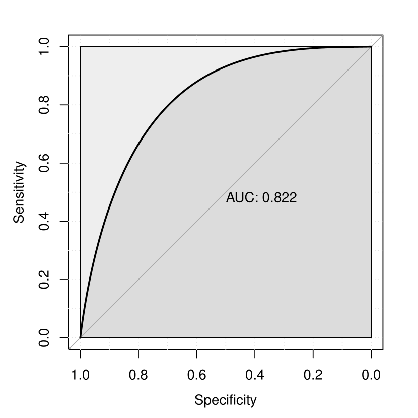
(a) ROC of proposed method

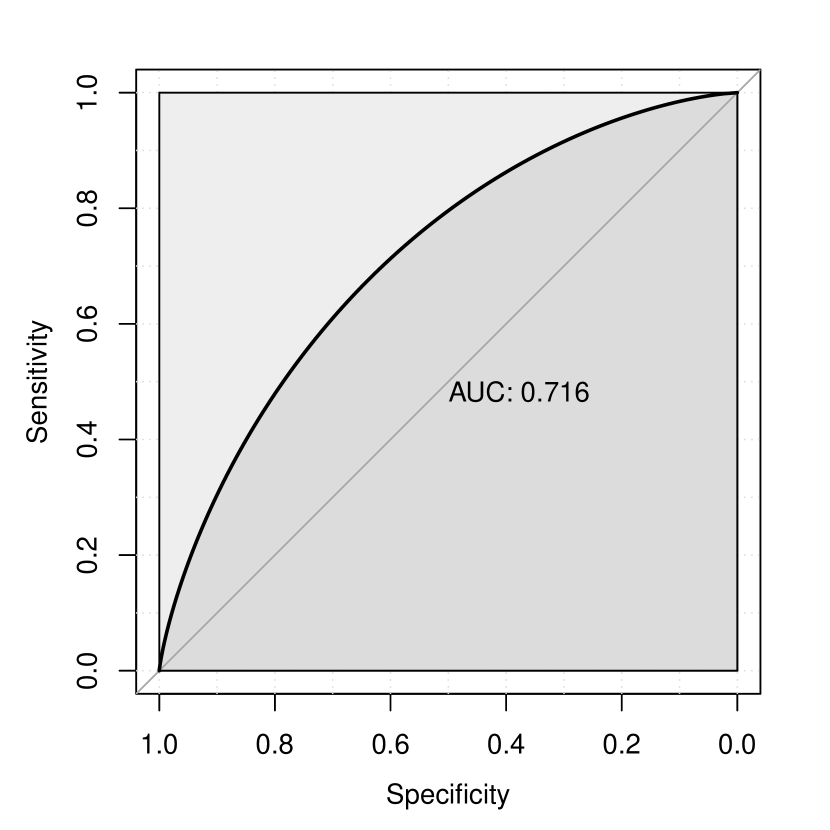
(b) ROC of logistic model

Figure 1. The ROC plots with Case I and $\delta=0.1$ in the simulation.

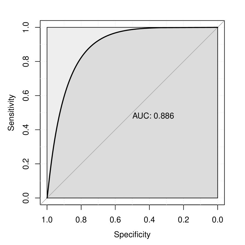
(a) ROC of proposed method

(b) ROC of logistic model

Figure 2. The ROC plots with Case I and $\delta=0.3$ in the simulation.

(a) ROC of proposed method

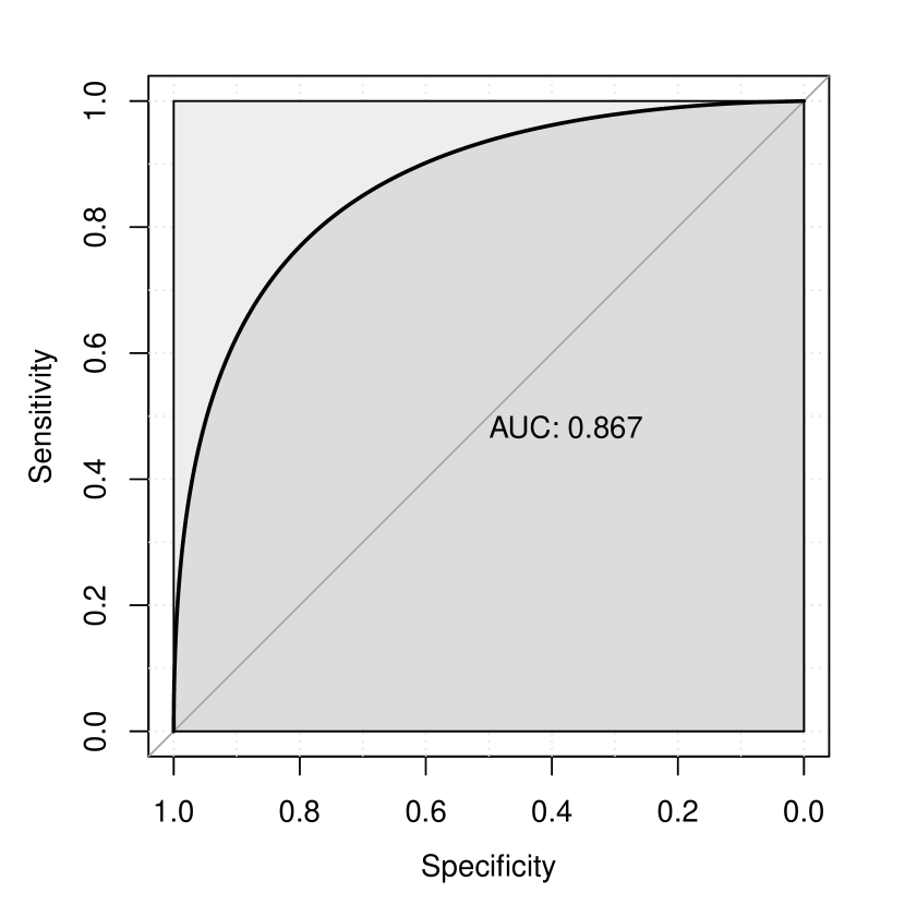
(b) ROC of logistic model

Figure 3. The ROC plots with Case II and $\delta=0.1$ in the simulation.

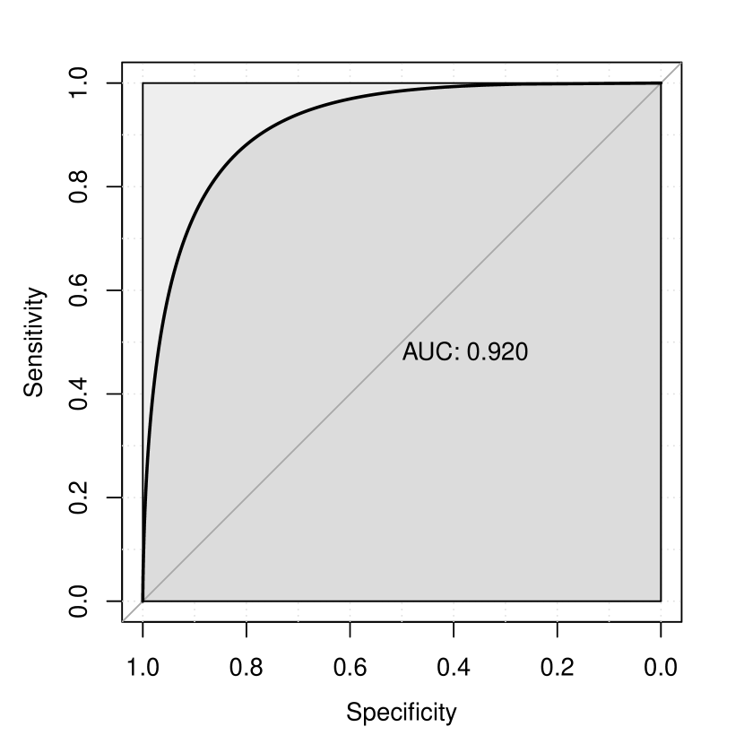
(a) ROC of proposed method

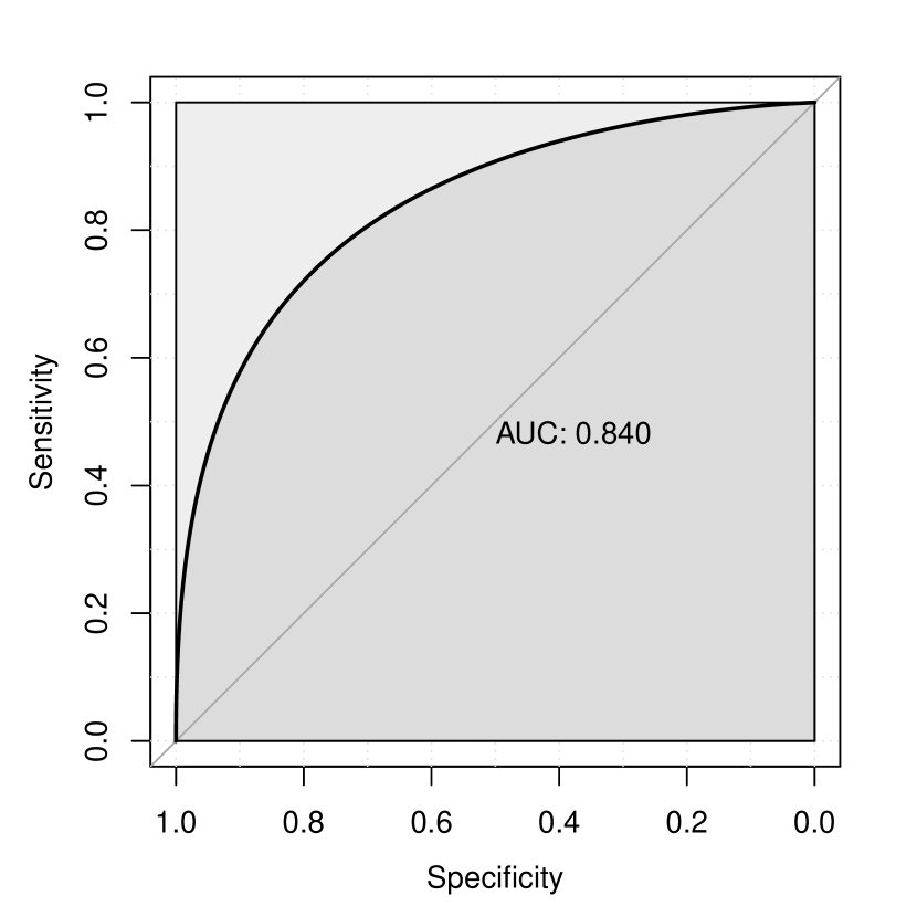
(b) ROC of logistic model

Figure 4. The ROC plots with Case II and $\delta=0.3$ in the simulation.

The receiver operating characteristic (ROC) curve is a very useful tool evaluate classifiers in many practical applications Fawcett (2006). In Figures 1-2, we report the ROC curves with $\delta=0.1$ (other cases are similar and omitted), which are plotted by the R package pROC Robin et al. (2011). From the view of ROC analysis, the area under the curve (AUC) measures the performance of a classifier. A larger value of AUC means a better classification capacity. In Figures 1-2 we also present the AUCs of two classifiers, which indicate the proposed method has a larger AUC compared with the classical logistic regression model. i.e., it is useful to use the network information when predicting the binary outcomes with our proposed model.

Figure 5. The plot of network for survival data in the Section 6.

6 Application

6.1 A generated network with survival data

In this section, we apply our proposed method to a generated network with survival data, which is available in the online supplemental material of Su et al. (2020). There are total 2000 nodes in the network ($n=2000$), and each node contains two covariates ($X_{i1}$ and $X_{i2}$), the observed failure time and censored indicator, where $X_{i1}$ is binary (e.g. male =1, female=0), $X_{i2}$ is continuous (e.g. age), $i=1,\cdots,n$. Denote the response $Y_{i}=1$ if the $i$th node is not censored, and $Y_{i}=0$ otherwise. The second variable $X_{2}$ is scaled with zero mean and unit variance. We use the proposed models (2.1) and (2.2) to analyse this network dataset. In Figure 3, we illustrate the above-mentioned network data in this application. It is clear that there are five communities in this network.

Table 4. The summary of parameter estimators in the Section 6.1^†. $\delta$ $\gamma_{0}$ $\gamma_{1}$ $\gamma_{2}$ $\beta_{0}$ $\beta_{1}$ $\beta_{2}$ Proposed 0.0275 -0.2861 3.3878 -1.7049 0.0495 1.1521 -0.6966 Logistic $*$ $*$ $*$ $*$ 0.3143 1.4415 -0.8353

$\dagger$ “Proposed” denotes our proposed method; “Logistic” denotes the the classical logistic regression model; “$*$” denotes the value is not available.

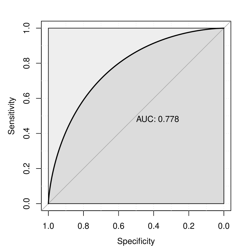
(a) ROC of proposed method

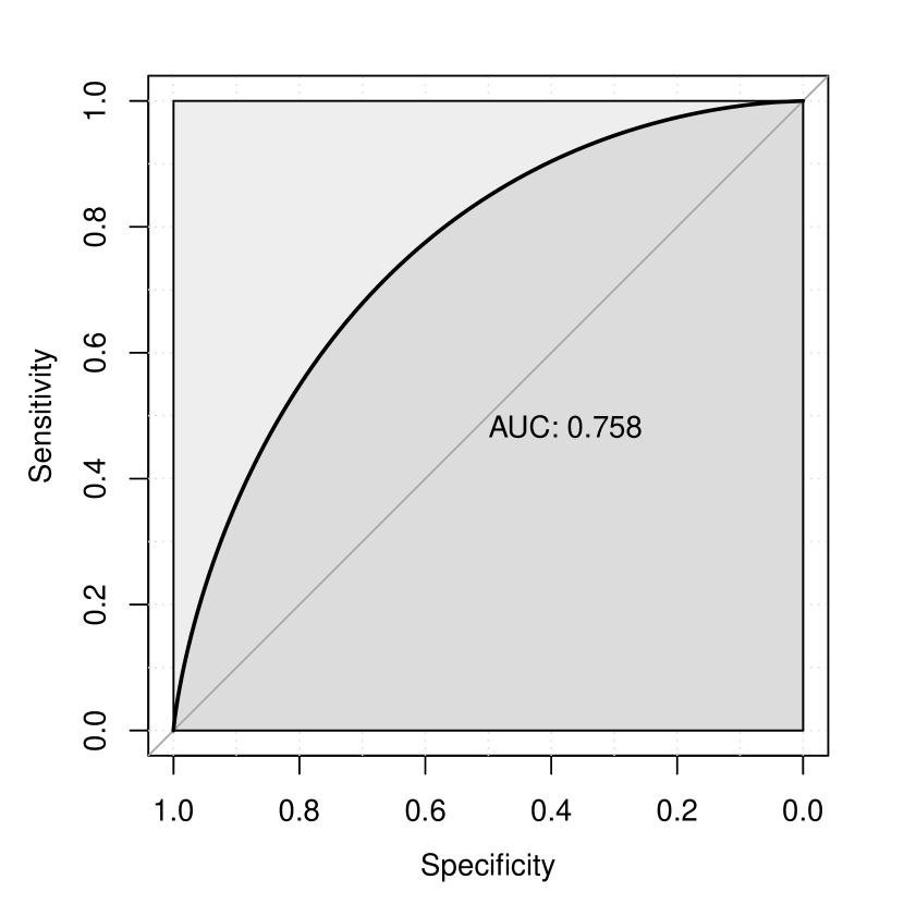
(b) ROC of logistic model

Figure 6. The ROC plots in the application (Section 6.1).

First we employ the proposed score test for $H_{0}:\delta=0$, where the perturbed test statistic $T_{n}^{*}$ is calculated 1000 times. At significance level $\alpha=0.05$, the empirical upper $\alpha$-quantile, $C_{\alpha}=9.44$, and the value of test statistic $T_{n}$ is 19.02. In view of the fact that $T_{n}>C_{\alpha}$, we can reject the null hypothesis $H_{0}$. i.e., there exists network dependence among nodes’ binary outcomes. Next, we estimate the model parameters by the proposed EM algorithm, where the results are presented in Table 4. The estimated parameter $\delta$ is 0.0275, indicating a significant positive network dependence among those susceptible nodes. For comparison, we also use the classical logistic model to fit this dataset, where the estimated parameters are given in Table 5. To evaluate the performance of classification, we report the ROC curves of both methods in Figure 4. Because the AUC of proposed method is larger than that of classical logistic model, our method is desirable to fit this network dataset. In addition, we calculate the estimated posterior “susceptible” probability for each node, where the histogram of the estimated posterior is reported in Figure 5. The majority of “susceptible” probabilities are large, indicating that those nodes are more likely to be influenced by their neighbors in the network.

Figure 7. Histogram of the estimated susceptible probabilities for the nodes in Section 6.1.

Figure 8. The plot of network for CiteSeer dataset in the Section 6.2.

6.2 The CiteSeer dataset with citation network

In this section, we apply our proposed method to the CiteSeer dataset, consisting of 3312 scientific publications classified into one of six classes. The datset is public available at https://linqs.soe.ucsc.edu/data. Every node (publication) in the dataset is described by a 0/1-valued word vector (features) indicating the absence/presence of the corresponding word from the dictionary with 3703 unique words. We use the PCA dimension reduction to obtain two covariates ($X_{i1}$ and $X_{i2}$) for each node. Denote the response $Y_{i}=1$ if the $i$th node is about artificial intelligence, and $Y_{i}=0$ otherwise. We use the proposed models (2.1) and (2.2) to analyse this network dataset. In Figure 8, we plot the CiteSeer dataset network, indicating this network is very sparse.

Table 5. The summary of parameter estimators in the Section 6.2^†. $\delta$ $\gamma_{0}$ $\gamma_{1}$ $\gamma_{2}$ $\beta_{0}$ $\beta_{1}$ $\beta_{2}$ Proposed 1.8986 -1.0855 -3.9585 6.1909 -2.4419 0.3034 -0.1540 Logistic $*$ $*$ $*$ $*$ -2.5526 0.3985 -0.3590

$\dagger$ “Proposed” denotes our proposed method; “Logistic” denotes the the classical logistic regression model; “$*$” denotes the value is not available.

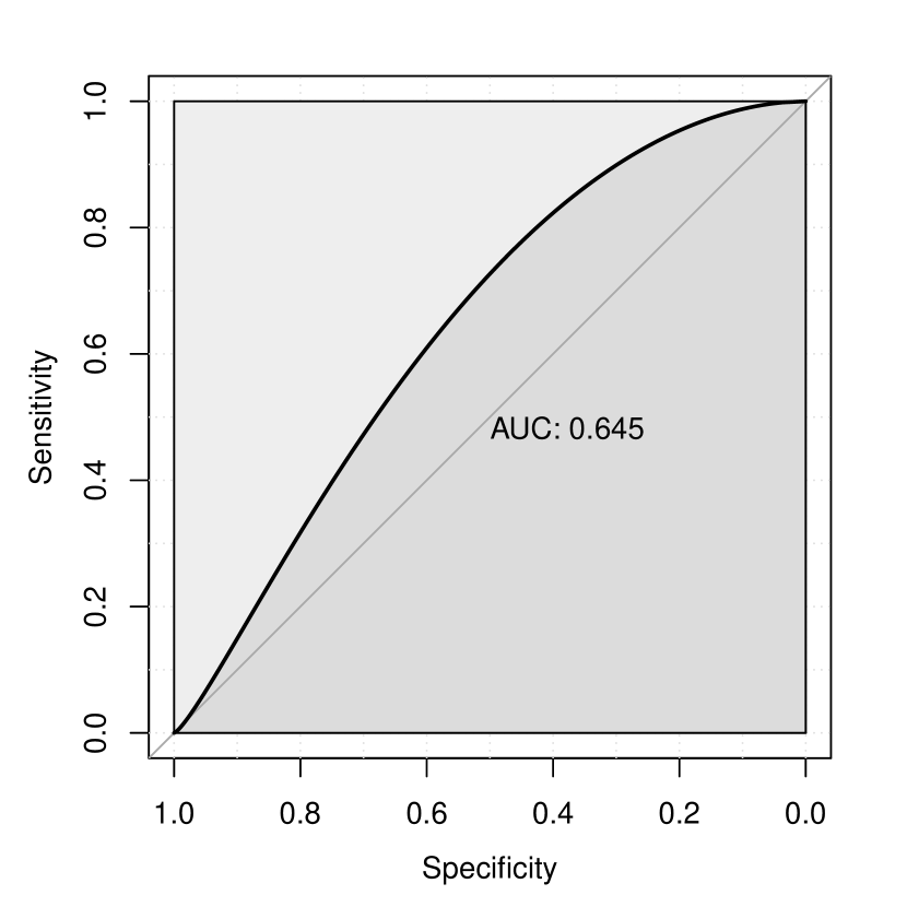
(a) ROC of proposed method

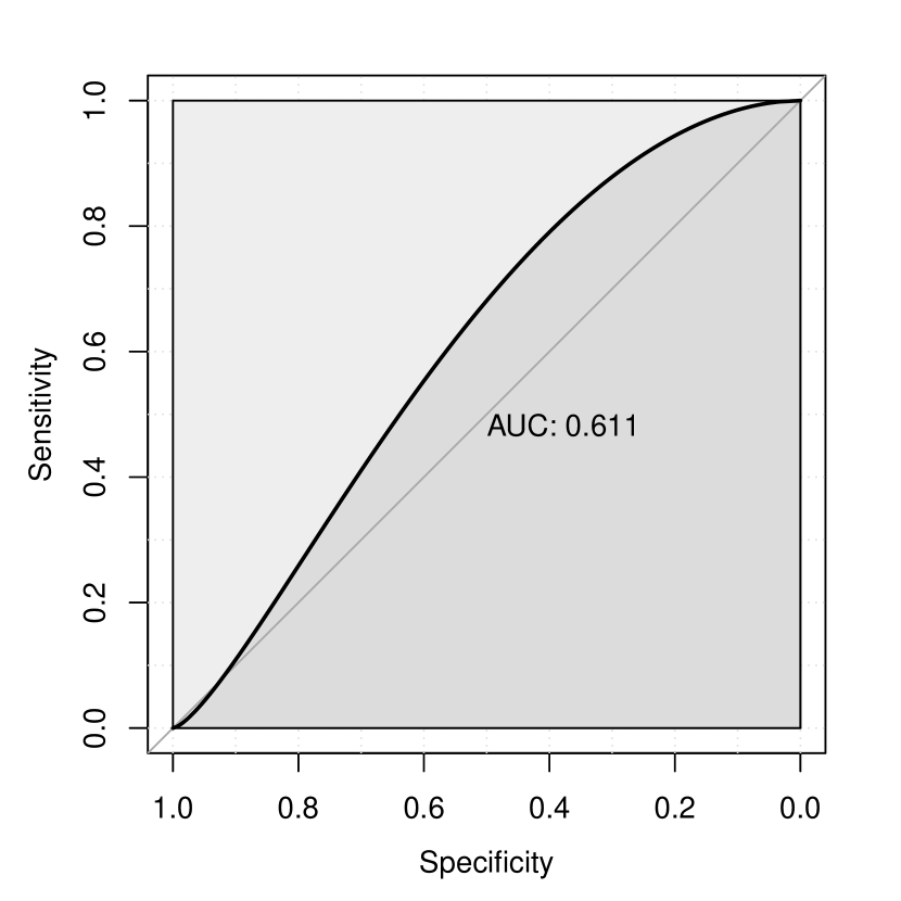
(b) ROC of logistic model

Figure 9. The ROC plots in the application (Section 6.2).

First we use the proposed score test for $H_{0}:\delta=0$, where the perturbed test statistic $T_{n}^{*}$ is calculated 1000 times. With significance level $\alpha=0.05$, the empirical upper $\alpha$-quantile, $C_{\alpha}=9.01$, and the value of test statistic $T_{n}$ is 41.20. Due to the fact that $T_{n}>C_{\alpha}$, we can reject the null hypothesis $H_{0}$. i.e., there exists network dependence among nodes’ binary outcomes. Next, we estimate the model parameters by the proposed EM algorithm, where the results are presented in Table 5. The estimated parameter $\delta$ is 1.8986, indicating a significant positive network dependence among those susceptible nodes. For comparison, we also use the classical logistic model to fit this dataset, where the estimated parameters are given in Table 6. To evaluate the performance of classification, we report the ROC curves of both methods in Figure 9. Because the AUC of proposed method is larger than that of classical logistic model, our method is desirable to fit this network dataset. Furthermore, we calculate the estimated posterior “susceptible” probability for each node, where the histogram of the estimated posterior is reported in Figure 10. The majority of “susceptible” probabilities are low for most nodes, but can be high for a group of node.

Figure 10. Histogram of the estimated susceptible probabilities for the nodes in Section 6.2.

7 Concluding Remarks

In this paper, we have proposed a novel latent logistic regression model to describe network dependence. We introduced a score-type test to check the existence of network dependence. An EM-type algorithm was used to estimate the model parameters. Simulations and applications were used to validate the usefulness of the proposed method. It is interesting to extend our idea to multi-class logistic regression model with graph data, which will be studied in the future of our research.

Appendix

Proof of Theorem 1: Note that $\tilde{{\bm{\eta}}}=(\tilde{\beta}_{0},\tilde{{\bm{\beta}}}^{\prime})^{\prime}$ is the standard maximum likelihood estimator with $\delta=0$, where the asymptotic property of $\tilde{{\bm{\eta}}}$ has been well established. By the Taylor expansion, we have

$$\frac{1}{\sqrt{n}}S^{*}(\tilde{{\bm{\theta}}};{\bm{\phi}})=\frac{1}{\sqrt{n}}S^{*}({\bm{\theta}}_{t};{\bm{\phi}})-\mathcal{B}^{*}_{n}({\bm{\theta}}_{t})\mathcal{I}_{n}^{-1}({\bm{\theta}}_{t})\frac{1}{\sqrt{n}}S_{1}({\bm{\theta}}_{t};{\bm{\phi}})+o_{P}(1),$$

where

$$S_{1}({\bm{\theta}}_{t};{\bm{\phi}}) = \frac{\partial L({\bm{\theta}};{\bm{\zeta}})}{\partial{\bm{\eta}}}|_{{\bm{\theta}}={\bm{\theta}}_{t}}$$

$$= \sum_{i=1}^{n}\left[Y_{i}-\frac{\exp(\beta_{0t}+\mathbf{X}_{i}^{\prime}{\bm{\beta}}_{t})}{1+\exp(\beta_{0t}+\mathbf{X}_{i}^{\prime}{\bm{\beta}}_{t})}\right](1,\mathbf{X}_{i}^{\prime})^{\prime}.$$

Hence, some calculations lead to the following expression:

$$\frac{1}{\sqrt{n}}S^{*}(\tilde{{\bm{\theta}}};{\bm{\phi}}) = \frac{1}{\sqrt{n}}\sum_{i=1}^{n}\tilde{Z}^{*}_{i}\left[Y_{i}-\frac{\exp(\beta_{0t}+\mathbf{X}_{i}^{\prime}{\bm{\beta}}_{t})}{1+\exp(\beta_{0t}+\mathbf{X}_{i}^{\prime}{\bm{\beta}}_{t})}\right]$$

$$-\mathcal{B}^{*}_{n}({\bm{\theta}}_{t})\mathcal{I}_{n}^{-1}({\bm{\theta}}_{t})\frac{1}{\sqrt{n}}\sum_{i=1}^{n}\left[Y_{i}-\frac{\exp(\beta_{0t}+\mathbf{X}_{i}^{\prime}{\bm{\beta}}_{t})}{1+\exp(\beta_{0t}+\mathbf{X}_{i}^{\prime}{\bm{\beta}}_{t})}\right](1,\mathbf{X}_{i}^{\prime})^{\prime}+o_{P}(1)$$

$$= \frac{1}{\sqrt{n}}\sum_{i=1}^{n}U_{i}^{*}({\bm{\theta}}_{t};{\bm{\phi}})+o_{P}(1).$$

Under some regularity conditions, it can be proved that $\sigma^{2}({\bm{\phi}})=\lim_{n\rightarrow\infty}n^{-1}\sum_{i=1}^{n}\{U_{i}^{*}({\bm{\theta}}_{t};{\bm{\phi}})\}^{2}$ is finite and can be consistently estimated by $n^{-1}\sum_{i=1}^{n}\{U_{i}^{*}(\tilde{{\bm{\theta}}};{\bm{\phi}})\}^{2}$. For fixed ${\bm{\phi}}$, we get that as $n\rightarrow\infty$,

$$n^{-1/2}S^{*}(\tilde{{\bm{\theta}}};{\bm{\phi}})\stackrel{{\scriptstyle d}}{{\longrightarrow}}N(0,\sigma^{2}({\bm{\phi}})),$$

where $\stackrel{{\scriptstyle d}}{{\longrightarrow}}$ denotes convergence in distribution. Moreover, we can derive that $n^{-1/2}S^{*}(\tilde{{\bm{\theta}}};{\bm{\phi}})$ converges in distribution to a Gaussian process with mean 0 and covariance matrix
$\lim_{n\rightarrow\infty}n^{-1}\sum_{i=1}^{n}U_{i}^{*}({\bm{\theta}}_{t};{\bm{\phi}}_{1})U_{i}^{*}({\bm{\theta}}_{t};{\bm{\phi}}_{2})$ for any ${\bm{\phi}}_{1}$, ${\bm{\phi}}_{2}\in{\bm{\Gamma}}$. This ends the proof.

References

• Carroll and Pederson (1993) Carroll, R. J. and Pederson, S. (1993). On robustness in the logistic regression model. Journal of the Royal Statistical Society: Series B (Methodological) 55, 693–706.
• Chandna et al. (2021) Chandna, S., Olhede, S., and Wolfe, P. (2021). Local linear graphon estimation using covariates. Biometrika DOI:10.1093/biomet/asab057.
• Conroy and Sajda (2012) Conroy, B. and Sajda, P. (2012). Fast, exact model selection and permutation testing for l2-regularized logistic regression. Proceedings of the Fifteenth International Conference on Artificial Intelligence and Statistics 22, 246–254.
• Das et al. (2013) Das, S., Moore, T., Wong, W., Stumpf, S., Oberst, I., McIntosh, K., and Burnett, M. (2013). End-user feature labeling: Supervised and semi-supervised approaches based on locally-weighted logistic regression. Artificial Intelligence 204, 56–74.
• Efron (1988) Efron, B. (1988). Logistic regression, survival analysis, and the kaplan-meier curve. Journal of the American statistical Association 83, 414–425.
• Fan et al. (2017) Fan, A., Song, R., and Lu, W. (2017). Change-plane analysis for subgroup detection and sample size calculation. Journal of the American Statistical Association 112, 769–778.
• Fawcett (2006) Fawcett, T. (2006). An introduction to roc analysis. Pattern Recognition Letters 27, 861–874.
• Han et al. (2019) Han, K., Hong, S., Cheon, J. H., and Park, D. (2019). Logistic regression on homomorphic encrypted data at scale. Proceedings of the AAAI Conference on Artificial Intelligence 33, 9466–9471.
• Holland et al. (1983) Holland, P., Laskey, K., and Leinhardt, S. (1983). Stochastic blockmodels: First steps. Social networks 5, 109–137.
• Jennings (1986) Jennings, D. (1986). Outliers and residual distributions in logistic regression. Journal of the American Statistical Association 81, 987–990.
• Landwehr et al. (1984) Landwehr, J. M., Pregibon, D., and Shoemaker, A. C. (1984). Graphical methods for assessing logistic regression models. Journal of the American Statistical Association 79, 61–71.
• Lemon et al. (2003) Lemon, S., Roy, J., Clark, M., Friedmann, P., and Rakowski, W. (2003). Classification and regression tree analysis in public health: Methodological review and comparison with logistic regression. Annals of Behavioral Medicine 26, 172–181.
• Li et al. (2019) Li, Y., Bellotti, T., and Adams, N. (2019). Issues using logistic regression with class imbalance, with a case study from credit risk modelling. Foundations of Data Science 1, 389–417.
• Liu et al. (2009) Liu, J., Chen, J., and Ye, J. (2009). Large-scale sparse logistic regression. Proceedings of the 15th ACM SIGKDD international conference on Knowledge discovery and data mining 547–556.
• Lu and Yang (2012) Lu, M. and Yang, W. (2012). Multivariate logistic regression analysis of complex survey data with application to BRFSS data. Journal of Data Science 10, 157–173.
• Meier et al. (2008) Meier, L., Geer, S. V. D., and Buhlmann, P. (2008). The group lasso for logistic regression. Journal of the Royal Statistical Society: Series B (Methodological) 70, 53–71.
• Pan et al. (2022) Pan, R., Chang, X., Zhu, X., and Wang, H. (2022). Link prediction via latent space logistic regression model. Statistics and Its Interface 15, 267–282.
• Pyke and Sheridan (1993) Pyke, S. and Sheridan, P. (1993). Logistic regression analysis of graduate student retention. Canadian Journal of Higher Education 23, 44–64.
• Robin et al. (2011) Robin, X., Turck, N., Hainard, A., Tiberti, N., Lisacek, F., Sanchez, J.-C., and Muller, M. (2011). proc: an open-source package for r and s+ to analyze and compare roc curves. BMC Bioinformatics 12:77.
• Schein and Ungar (2007) Schein, A. and Ungar, L. (2007). Active learning for logistic regression: an evaluation. Machine Learning 68, 235–265.
• Shi et al. (2010) Shi, J., Yin, W., Osher, S., and Sajda, P. (2010). A fast hybrid algorithm for large-scale l1-regularized logistic regression. Journal of Machine Learning Research 11, 713–741.
• Singh et al. (2009) Singh, S., Kubica, J., Larsen, S., and Sorokina, D. (2009). Parallel large scale feature selection for logistic regression. Proceedings of the 2009 SIAM International Conference on Data Mining (SDM) 1172–1183.
• Stefanski and Carroll (1985) Stefanski, L. A. and Carroll, R. J. (1985). Covariate measurement error in logistic regression. Annals of Statistics 13, 1335–1351.
• Su et al. (2020) Su, L., Lu, W., Song, R., and Huang, D. (2020). Testing and estimation of social network dependence with time to event data. Journal of the American Statistical Association 115, 570–582.
• Tripathi et al. (2017) Tripathi, Y., Mahto, A., and Dey, S. (2017). Efficient estimation of the PDF and the CDF of a generalized logistic distribution. Annals of Data Science 4, 63–81.
• Wang (2020) Wang, H. (2020). Logistic regression for massive data with rare events. Proceedings of the 37th International Conference on Machine Learning 119, 9829–9836.
• Wang et al. (2018) Wang, H., Zhu, R., and Ma, P. (2018). Optimal subsampling for large sample logistic regression. Journal of the American Statistical Association 113, 522, 829–844.
• Wu et al. (2009) Wu, T. T., Chen, Y. F., Hastie, T., Sobel, E., and Lange, K. (2009). Genome-wide association analysis by lasso penalized logistic regression. Bioinformatics 25, 714–721.
• Yan et al. (2019) Yan, T., Jiang, B., Fienberg, S., and Leng, C. (2019). Statistical inference in a directed network model with covariates. Journal of the American Statistical Association 114, 857–868.
• Yang and Loog (2018) Yang, Y. and Loog, M. (2018). A benchmark and comparison of active learning for logistic regression. Pattern Recognition 83, 401–415.
• Yuan et al. (2012) Yuan, G., Ho, C., and Lin, C. (2012). An improved glmnet for L1-regularized logistic regression. Journal of Machine Learning Research 13, 1999–2030.
• Zhang et al. (2022) Zhang, H., Guo, X., and Chang, X. (2022). Randomized spectral clustering in large-scale stochastic block models. Journal of Computational and Graphical Statistics DOI: 10.1080/10618600.2022.2034636.
• Zhao et al. (2022) Zhao, J., Liu, X., Wang, H., and Leng, C. (2022). Dimension reduction for covariates in network data. Biometrika 109, 85–102.
• Zhu et al. (2021) Zhu, X., Cai, Z., and Ma, Y. (2021). Network functional varying coefficient model. Journal of the American Statistical Association DOI: 10.1080/01621459.2021.1901718.
• Zhu et al. (2017) Zhu, X., Pan, R., Li, G., Liu, Y., and Wang, H. (2017). Network vector autoregression. Annals of Statistics 43, 1096–1123.
• Zuo et al. (2021) Zuo, L., Zhang, H., Wang, H., and Sun, L. (2021). Optimal subsample selection for massive logistic regression with distributed data. Computational Statistics 36, 2535–2562.