Kernelized multi-graph matching

Abstract

Multigraph matching is a recent variant of the graph matching problem. In this framework, the optimization procedure considers several graphs and enforces the consistency of the matches along the graphs. This constraint can be formalized as a cycle consistency across the pairwise permutation matrices, which implies the definition of a universe of vertex (Pachauri et al., 2013). The label of each vertex is encoded by a sparse vector and the dimension of this space corresponds to the rank of the bulk permutation matrix, the matrix built from the aggregation of all the pairwise permutation matrices. The matching problem can then be formulated as a non-convex quadratic optimization problem (QAP) under constraints imposed on the rank and the permutations. In this paper, we introduce a novel kernelized multigraph matching technique that handles vectors of attributes on both the vertices and edges of the graphs, while maintaining a low memory usage. We solve the QAP problem using a projected power optimization approach and propose several projectors leading to improved stability of the results. We provide several experiments showing that our method is competitive against other unsupervised methods.

1 Introduction & Related work

Graph matching is general problem with many applications such as e.g. object recognition and registration, or shape matching to cite a few. Let $G_{1}$ and $G_{2}$ be two graphs with respectively $n_{1}$ and $n_{2}$ vertices. The pairwise matching problem is often cast as a quadratic assignment problem (QAP), using the Lawler’s formula (Lawler, 1963),

$$\max_{X\in\mathcal{P}_{n_{1},n_{2}}}{\mathrm{vec}(X)}^{T}K^{e}\mathrm{vec}(X)+\mathrm{tr}(K^{v}X)\leavevmode\nobreak\ ,$$ (1)

with $\mathcal{P}_{n_{1},n_{2}}$ the set of permutation matrix of size $n_{1}\times n_{2}$, $K^{v}\in\mathbb{R}^{n_{1}\times n_{2}}$ the vertex affinity matrix and $K^{e}\in\mathbb{R}^{n_{1}n_{2}\times n_{1}n_{2}}$ the edge affinity matrix. These affinity matrices can be built using kernels, then $K^{v}$ and $K^{e}$ are both Gram matrix build using respectively a vertex kernel and an edge kernel (Zhang et al., 2019).

As $K^{e}$ could be a very large matrix, usually the Koopmans-Beckmann’s QAP (Koopmans and Beckmann, 1957) is preferred,

$$\max_{X\in\mathcal{P}_{n_{1},n_{2}}}\mathrm{tr}(XA_{1}XA_{2})+\mathrm{tr}(K^{v}X)\leavevmode\nobreak\ ,$$ (2)

with $A_{1}$ and $A_{2}$ respectively the adjacency matrices of $G_{1}$ and $G_{2}$. (2) is a special case of Lawler’s QAP with $K^{e}=A_{1}\otimes A_{2}$ (the Kronecker product between the two adjacency matrices).

Recently, Zhang et al. (2019) showed that by using specific kernels for computing the edge affinity matrix, (1) has a more memory manageable writing. Furthermore, their formulation with kernels allows to match a large diversity of graphs, as kernels can easily manage labels or vectors of attributes. They also propose a regularization scheme combined with a Frank-Wolfe optimization leading to very good performances compared to state of the art methods and good robustness to noise both on attributes and structure.

Multigraph matching is an extension of the graph matching problem, where one aims at matching several graphs at once while enforcing coherence between the vertex assignments. In order to enforce the coherence, the idea is to search for a cycle consistency (Pachauri et al., 2013) between the permutation matrices, i.e. if $X_{i,j}$ is the permutation matrix between graphs $i$ and $j$, for a graph $k$ we have $X_{i,j}\approx X_{i,k}X_{k,j}$. It is an approximation since the graphs may not have the same number of vertices.

Pachauri et al. (2013) showed that the cycle consistency property is equivalent to projecting the vertices into a discrete space. A matching between two vertices means that they have the same image in this space. The dimension of this space is directly linked to the diversity of the vertices in the set of graphs. This diversity reflects the attributes and/or labels that are defined on the vertices. Recent methods like MatchALS (Zhou et al., 2015) implicitly use it by minimizing the rank the bulk permutation matrix. Some others such as HiPPI (Bernard et al., 2019) and GA-MGM (Wang et al., 2020a) directly run the optimization in the universe of vertex. On the other side CAO (Yan et al., 2015) and Floyd (Jiang et al., 2020) optimize both affinity and the cycle consistency using a graduated scheme. MLRWM-multi (Park and Yoon, 2016), a multigraph extension of RRWM (Cho et al., 2010) is based on a multi-layer approach to ensure vertex consistency. Most of these methods relies on non-convex optimization as convex relaxation is not trivial (Fogel et al., 2013; Swoboda et al., 2019) and may lead to inappropriate solutions in some cases (Aflalo et al., 2015; Lyzinski et al., 2015). While there is now many works using deep learning methods (Fey et al., 2020; Wang et al., 2020b; Rolínek et al., 2020; Wang et al., 2021; Liu et al., 2021b) for graph matching only a few tackle the multi-graph matching problem.

In this paper we focus on the unsupervised version of the multigraph matching problem that is faced in the many applications where no ground truth labeling is available. We propose an extended version of the framework proposed for KerGM (Zhang et al., 2019) for multigraph matching with an appropriate projection to fulfill the constraints. The induced optimization problem is solved using recent non-convex optimization scheme which guarantees convergence under mild condition. Results on classic data set show promising results compared to other state-of-art unsupervised methods.

Our main contributions are:

• An unsupervised multigraph matching method based on Lawler’s QAP which allows kernel over both edge and vertex attributes while keeping a tractable computer memory load.

• A flexible algorithm which allows a set of projection power to find cycle consistent permutation matrices.

• Experiments on real data-sets demonstrating that our approach is competitive with state-of-art results.

2 Preliminaries about array operations and multi-graph matching

Let $\{G_{i}\}_{i=1\ldots n}$ be a set of $n$ graphs with $\forall i,G_{i}=\{V_{i},E_{i}\subseteq V_{i}\times V_{i},L^{v},L^{e}\}$, i.e. a graph is defined by a set of vertices, a set of edges and two functions: $L^{v}:V\mapsto\mathbb{R}^{d_{v}}$ which gives the data vector associated to a vertex and $L^{e}:E\mapsto\mathbb{R}^{d_{e}}$ which gives the data vector associated to an edge. We also define $\boldsymbol{\mathrm{I}}_{m}$ as the identity matrix of size $m$ and $\mathbb{1}_{m}$ the vector of $1$ of size $m$. For a matrix $X\in\mathbb{R}^{n\times n}$, we denote for $i,j\in\{1,\ldots,n\}$ by $X[i,j]$ the scalar at line $i$ and column $j$, and by $X[:,j]$ we denote the vector form by column $j$ (and reciprocally for lines). First we introduce the notion of array operations in Hilbert space, these tools will be useful to factorize (1) the edge affinity matrices.

2.1 Array operations in Hilbert space

We propose a rapid and simplified introduction to $\mathcal{H}$-operations arrays in Hilbert spaces presented in Zhang et al. (2019). Let $\Phi,\Psi\in\mathbb{R}^{d\times m\times m}$ be 3d-arrays (or 3d-matrices). For $\Phi\in\mathbb{R}^{d\times m\times m}$, we denote by $\Phi[l,i,j]\in\mathbb{R}$ the scalar at coordinates $l,i,j$ and by $\Phi[:,i,j]\in\mathbb{R}^{d}$ the vector at the coordinates $i,j$. $\forall X\in\mathbb{R}^{m\times m}$ we define the following operations,

1. $\Phi^{T}\in\mathbb{R}^{d\times m\times m}$ with $\forall i,j,\ \Phi[:,i,j]=\Phi[:,j,i]$ (i.e. the transpose operation along the two last axis).

2. $\Phi*\Psi\in\mathbb{R}^{m\times m}$ where $\forall i,j$,

   $$[\Phi*\Psi][i,j]=\sum_{k=1}^{m}\left\langle\Phi[:,i,k],\Psi[:,k,j]\right\rangle=\sum_{k=1}^{m}\sum_{l=1}^{d}\Phi[l,i,k]\Psi[l,k,j]\leavevmode\nobreak\ .$$

3. $\forall X\in\mathbb{R}^{d\times m\times m}$, $\Phi\odot X\in\mathbb{R}^{m\times m}$ where $\forall i,j$,

   $$[\Phi\odot X][i,j]=\sum_{k=1}^{m}\Phi[:,i,k]X[k,j]=\sum_{k=1}^{m}X[k,j]\Phi[:,i,k]\leavevmode\nobreak\ .$$

   Similarly, we define $X\odot\Phi\in\mathbb{R}^{m\times m}$ where,

   $$\forall i,j,\ [X\odot\Phi][i,j]=\sum_{k=1}^{m}X[i,k]\Phi[:,k,j]\leavevmode\nobreak\ .$$

The last operator can be read as a parallelized matrix product over the first axis.

We recap several results from Zhang et al. (2019) with the following proposition,

Proposition 2.1 (Zhang et al. (2019)).

Define the function $\left\langle.,.\right\rangle:\mathbb{R}^{d\times m\times m}\times\mathbb{R}^{d\times m\times m}\to\mathbb{R}$ such that $\forall\Phi,\Psi\in\mathbb{R}^{d\times m\times m}$, $\left\langle\Phi,\Psi\right\rangle=\mathrm{tr}(\Phi^{T}*\Psi)$. Then $\left\langle.,.\right\rangle$ is a inner product on $\mathbb{R}^{d\times m\times m}$ and the following equalities are true,

• Let $\Phi,\Psi\in\mathbb{R}^{d\times m\times m}$, we have $\forall X\in\mathbb{R}^{m\times m}$, $\left\langle\Phi\odot X,\Psi\right\rangle=\left\langle\Phi,\Psi\odot X^{T}\right\rangle$ and $\left\langle X\odot\Phi,\Psi\right\rangle=\left\langle\Phi,X^{T}\odot\Psi\right\rangle$ .

• $\forall X,Y\in\mathbb{R}^{m\times m}$, $\Phi\in\mathbb{R}^{d\times m\times m}$, we have, $\Phi\odot X\odot Y=\Phi\odot(XY)$, and $Y\odot(X\odot\Phi)=(YX)\odot\Phi$ .

• Let $\Phi,\Psi\in\mathbb{R}^{d\times m\times m}$, we have $\forall X\in\mathbb{R}^{m\times m}$, $\left\langle\Phi,\Psi\odot X\right\rangle=\left\langle\Psi^{T}*\Phi,X\right\rangle$ and $\left\langle\Phi,X\odot\Psi\right\rangle=\left\langle\Phi*\Psi^{T},X\right\rangle$ .

2.2 Building the optimization problem

We assume that the graphs have the same number of vertices $m>0$, we add dummy vertices if necessary. We define the constraints on cycle consistency in Definition 2.2.

Definition 2.2 (Cycle-consistency (Bernard et al., 2019)).

Let $\mathcal{X}=\{X_{i,j}\in\mathcal{P}_{m,m}\}^{n}_{i,j=1}$ be the set of pairwise matchings in a collection of $n$ objects, where each $X_{i,j}$ is an element of the set of partial permutation matrices,

$$\mathcal{P}_{m,q}=\{X\in\{0,1\}^{m\times q}\ :\ X\mathbb{1}_{q}\leq\mathbb{1}_{m},X^{T}\mathbb{1}_{m}\leq\mathbb{1}_{q}\}\leavevmode\nobreak\ .$$ (3)

The set $\mathcal{X}$ is said to be cycle-consistent if for all $i,j,l\in\{1,\ldots,k\}$ it holds that: (i) $X_{i,i}=\boldsymbol{\mathrm{I}}_{m}$ (identity matching), (ii) $X_{i,j}=X^{T}_{j,i}$ (symmetry), and (iii) $X_{i,j}X_{j,l}\leq X_{i,l}$ (transitivity).

The inequalities in this definition allows graphs of different sizes.

From Definition 2.2, Bernard et al. (2019) formalized the links with the universe of vertices with the following lemma,

Lemma 2.3 (Cycle-consistency, universe points (Bernard et al., 2019)).

The set $\mathcal{X}$ of pairwise matchings is cycle-consistent, if there exists a collection of rank $r$ $\{X_{l}\in\mathcal{P}_{m,r}\ :\ X_{l}\mathbb{1}_{r}=\mathbb{1}_{m}\}^{n}_{l=1}$, such that for each $X_{i,j}\in\mathcal{X}$ it holds that $X_{i,j}=X_{i}X_{j}^{T}$.

Notice that the universe of vertices can be seen as a discrete embedding space for vertices.

From Lemma 2.3 and using matrix factorization, we build our constraint set as follows,

$$\mathcal{C}_{r}=\{X\in\mathbb{R}^{nm\times nm}\ :\ X_{i,i}=\boldsymbol{\mathrm{I}}_{m},X_{i,j}=X^{T}_{j,i}=X_{i}X_{j}^{T}\text{ with }X_{i}\in\mathcal{P}_{m,r}\}\leavevmode\nobreak\ .$$ (4)

This formulation implies that $X\in\mathcal{C}_{r}$ is of rank $r$.

Let $K^{v}\in\mathbb{R}^{mn\times mn}$ be the full vertex affinity matrix built using a kernel on vertices where each block $K^{v}_{i,j}\in\mathbb{R}^{m\times m}$ is the Gram matrix of a vertex kernel applied on the data vectors (through $L^{v}$) on vertices of $G_{i}$ and $G_{j}$. Let $K^{e}\in\mathbb{R}^{mn^{2}\times mn^{2}}$ be the full edge affinity matrix built using a kernel on edges. Using the Lawler’s QAP, we aim to solve,

$$\max_{X\in\mathcal{C}_{r}}{\mathrm{vec}(X)}^{T}K^{e}\mathrm{vec}(X)+\mathrm{tr}(K^{v}X)\leavevmode\nobreak\ .$$ (5)

3 Proposed approach

The limitation with (5) is the size of $K^{e}$ which may be very large. In order to address this limitation, we use the framework proposed in Section 2.1 (following the ideas from Zhang et al. (2019)) to rewrite $K^{e}$ by factorizing it using a array $\Phi$ such that,

$${\mathrm{vec}(X)}^{T}K^{e}\mathrm{vec}(X)=\left\langle\Phi\odot X,X\odot\Phi\right\rangle\leavevmode\nobreak\ .$$ (6)

To build $\Phi$, we need to define it for each graph. For graph $G_{k}$, let $\Phi_{k}^{d\times m\times m}$ be defined as follows,

$$\Phi_{k}[i,j]=\begin{cases}L^{e}(v_{i},v_{j})=\phi_{i,j}\in\mathbb{R}^{d}\quad&\text{if }(v_{i},v_{j})\in E_{k}\leavevmode\nobreak\ ,\\ 0\quad&\text{otherwise}\leavevmode\nobreak\ .\end{cases}$$ (7)

$\phi_{i,j}$ is the data vector on the edge $(v_{i},v_{j})$. There many way to build these vectors, for example Gaussian kernels can be approximated using Random Fourier Features (Rahimi and Recht, 2007) (see also (Liu et al., 2021a) for other kernel approximations). Then $\Phi\in\mathbb{R}^{d\times nm\times nm}$ is given by the 3d-array with the $\Phi_{k}$ on the diagonal,

$$\Phi=\left(\begin{array}[]{ccc}\Phi_{1}&&0\\ &\Phi_{2}&\\ 0&&\ddots\end{array}\right)$$ (8)

This formulation has the advantage to be more compact than manipulating the full edge affinity matrix, since the size of $\Phi$ is $d\times nm\times nm$ compare to $(nm)^{2}\times(nm)^{2}$ for $K^{e}$.

Then we reformulate (5) as

$$\max_{X\in\mathcal{C}_{r}}J(X)=\left\langle\Phi\odot X,X\odot\Phi\right\rangle+\mathrm{tr}(K^{v}X)\leavevmode\nobreak\ .$$ (9)

This optimization problem is non-convex because of the two constraints (rank and permutation), we need then a dedicated scheme to solve it.

3.1 Optimization scheme

Since (9) is a quadratic optimization problem with non-convex constraints, we use a power optimization scheme. This scheme has the advantages to have almost no hyper-parameters and show rather fast convergence rate and the non-convex constraints are deal with a projector which gives an approximate solution. First we need the gradient of the objective function in (9).

Proposition 3.1.

The gradient of $J$ in (9) at $X$ is,

$$\nabla J(X)=K^{v}+(\Phi\odot X)*\Phi^{T}+\Phi^{T}*(X\odot\Phi)\leavevmode\nobreak\ .$$ (10)

Proof 3.2.

Let $J=J_{1}+J_{2}$ with $J_{1}(X)=\left\langle\Phi\odot X,X\odot\Phi\right\rangle$ and $J_{2}(X)=\mathrm{tr}(K^{v}X)$. By definition of the gradient we have,

$$\left\langle\nabla J_{1}(X),E\right\rangle=\lim_{t\to 0}\frac{1}{t}(J_{1}(X+tE)-J_{1}(X))\leavevmode\nobreak\ .$$

Using Proposition 2.1 we have,

$$J_{1}(X+tE) =\left\langle\Phi\odot(X+tE),(X+tE)\odot\Phi\right\rangle\leavevmode\nobreak\ ,$$

$$=\left\langle\Phi\odot X+t\Phi\odot E,X\odot\Phi+tE\odot\Phi\right\rangle\leavevmode\nobreak\ ,$$

$$=\left\langle\Phi\odot X,X\odot\Phi\right\rangle+t\left\langle\Phi\odot E,X\odot\Phi+tE\odot\Phi\right\rangle\leavevmode\nobreak\ ,$$

$$=\left\langle\Phi\odot X,X\odot\Phi\right\rangle+t\left\langle\Phi\odot X,E\odot\Phi\right\rangle+t\left\langle\Phi\odot E,X\odot\Phi\right\rangle+$$

$$\qquad t^{2}\left\langle\Phi\odot E,E\odot\Phi\right\rangle\leavevmode\nobreak\ .$$

From the gradient definition we yield,

$$\left\langle\nabla J_{1}(X),E\right\rangle =\left\langle\Phi\odot X,E\odot\Phi\right\rangle+\left\langle\Phi\odot E,X\odot\Phi\right\rangle\leavevmode\nobreak\ ,$$

$$=\left\langle(\Phi\odot X)*\Phi^{T}+\Phi^{T}*(X\odot\Phi),E\right\rangle\leavevmode\nobreak\ .$$

By identification we have $\nabla J_{1}(X)=(\Phi\odot X)*\Phi^{T}+\Phi^{T}*(X\odot\Phi)$. As the gradient of $J_{2}(X)=\mathrm{tr}(K^{v}X)$ is $\nabla J_{2}(X)=K^{v}$, we produce (10).

With the gradient we can solve (9) using a power method scheme. The full method is described in Algorithm 1. Since the gradient is a proxy for the quadratic operator, this scheme is closely related to HiPPI (Bernard et al., 2019). Assuming that we are able to solve the projection step, the scheme converges to a stationary point.

Proposition 3.3.

Algorithm 1 produces a monotone sequence and converges to a stationary point in a finite number of steps.

Proof 3.4.

This proof relies on the same arguments as for HiPPI (Bernard et al., 2019) for its Proposition 3. Let $\mathcal{U}=\mathrm{conv}(\mathcal{C}_{r})$ (the convex hull of the constraint set). We can relax (9) in

$$\max_{X\in\mathcal{U}}\left\langle\Phi\odot X,X\odot\Phi\right\rangle+\mathrm{tr}(K^{v}X) =\max_{X\in\mathcal{U}}\mathrm{vec}(X)^{T}K^{e}\mathrm{vec}(X)+\mathrm{tr}(K^{v}X),$$

$$\equiv\min_{X\in\mathbb{R}^{nm\times mn}}\imath_{\mathcal{U}}(X)-\underbrace{\mathrm{vec}(X)^{T}\tilde{K}\mathrm{vec}(X)}_{h(X)}\leavevmode\nobreak\ ,$$ (11)

with $\imath_{\mathcal{U}}$ the convex indicator function of set $\mathcal{U}$ (i.e. it return 0 for element from $\mathcal{U}$ and $+\infty$ otherwise) and $\tilde{K}$ the matrix compound of $K^{e}$ with the addition of $\mathrm{vec}(K^{v})$ on the diagonal. Since (11) is a difference of two convex functions we can apply difference of convex (DC) programming updates rules (Le Thi and Pham Dinh, 2018) with an initial step $X_{0}$,

$$V_{t} =\nabla_{X}h(X)=2\ \mathrm{unvec}(\tilde{K}\mathrm{vec}(X_{t}))\leavevmode\nobreak\ ,$$

$$X_{t+1} =\operatorname*{argmin}_{X\in\mathbb{R}^{nm\times nm}}\imath_{\mathcal{U}}(X)-h(X_{t})-\langle X-X_{t},V_{t}\rangle\leavevmode\nobreak\ ,$$

$$=\operatorname*{argmin}_{X\in\mathcal{U}}-\langle X,V_{t}\rangle\leavevmode\nobreak\ ,$$

where $\mathrm{unvec}$ is the inverse of $\mathrm{vec}$. $\mathcal{U}$ is linked with the Birkhoff polytope with the permutation matrix as extreme points (Maciel and Costeira, 2003; Birdal and Simsekli, 2019). Since the maximum of the linear objective over a compact set is attained at its extreme points, we get,

$$X_{t+1} =\operatorname*{argmin}_{X\in\mathcal{U}}-\langle X,V_{t}\rangle\leavevmode\nobreak\ ,$$

$$=\operatorname*{argmin}_{X\in\mathcal{U}}\|V_{t}-X\|^{2}_{F}=\mathrm{proj}_{\mathcal{C}_{r}}(V_{t})\leavevmode\nobreak\ ,$$

where $\langle X,X\rangle=nm$ since $X$ is formed from permutation matrices. Then we get from DC programming property that the sequence $\{X_{t}\}^{T}_{t=0}$ is a increasing sequence for $J$ in (9). Since $\mathcal{C}_{r}$ is a finite set, $J$ is bounded above for any $X\in\mathcal{C}_{r}$. Furthermore as $\forall t>0,X_{t}\in\mathcal{C}_{r}$, the increasing sequence $\{X_{t}\}^{T}_{t=0}$ converges to a stationary point.

Input : Affinity vertices matrix $K^{v}$, edges’ data 3d-array $\Phi$, tolerance $\tau$, maximal number of iterations $T$, rank $r$.

Output : $X_{T}$ the bulk permutation matrix.

$X_{0}\leftarrow 0$;

for $t\leftarrow 1$ to $T$ do

       $\hat{X}_{t}\leftarrow\nabla J(X_{t})$;

        // Using Proposition 3.1

       $X_{t+1}\leftarrow\text{proj}_{\mathcal{C}_{r}}(\hat{X}_{t})$;

       if $\|X_{t+1}-X_{t}\|<\tau$ then

             break;

            

       end if

      $t\leftarrow t+1$;

      

end for

Algorithm 1 Power method for solving (9)

Complexity of Algorithm 1: The computational complexity of the algorithm mainly depends on both the computation of the gradient and the projection onto the set of permutations. Since we are dealing with 3d-arrays of size $d\times m\times n$ the complexity of both $*$ and $\odot$ operations is $\mathcal{O}(d(nm)^{2})$. The complexity of the permutation depends on the selected approach to solve the optimization. We discuss this point in the next section.

Initialization: As many non-convex methods our method is sensitive to the initialization. For example methods like HiPPI (Bernard et al., 2019) or GA-MGM (Wang et al., 2020a) cannot start with an uniformly valued matrix. Since they are working in the universe of vertices, the initialization impacts the projection step and a method like the Hungarian method will just put the vertex in order (i.e. the vertex 1 will match other vertex 1 and so on). The algorithm ends-up being stuck in a solution where the permutation matrices are simply the identity. To avoid such an issue, GA-MGM for example, uses a random initialization, leading to a non deterministic optimization method. For our method such initialization is less a problem. If we initialize with the null matrix, the algorithm will only use the vertex affinity matrix to recover the permutations. Such initialization is relevant if the affinity is correctly tuned and it makes our method deterministic.

Comparison with closely related methods: While our method is not the first multi-graph method to include edge attributes, it is the first to propose a tractable way of dealing with real-world data. For example, methods like Floyd (Jiang et al., 2020) or deep learning methods like NGM (Wang et al., 2021) directly work with Lawler’s QAP (1). This leads to manipulate matrices whose size are quadratic in the number of vertices, so they only consider pairwise matching for most set of graphs. In comparison, with the arrays, we are able to manipulate matrices whose sizes linearly depends on the number of vertices. The cycle consistency constraints can then consider the full set of graphs.

3.2 Projection over the set of constraints

Optimizing on $\mathcal{C}_{r}$ is a NP-Hard problem. Furthermore as mentioned in several publications (Bernard et al., 2019; Shi et al., 2020), most of the approximation methods are very sensitive to the initialization and some require to provide a reference graph (mSync (Pachauri et al., 2013) for example). Recent methods include:

mSync

(Pachauri et al., 2013) uses an eigen decomposition and a reference graph (the first graph in the algorithm presented in the paper) combined with the Hungarian method to recover the permutations.

MatchEIG

(Maset et al., 2017) is an alternative to mSync with no reference graph but still combines eigen decomposition with the Hungarian method. As noticed in Bernard et al. (2021), the cycle consistency is not guaranteed.

Birkhoff-RLMC

(Birdal and Simsekli, 2019) uses a probabilistic method to estimate the permutation matrix from a noisy observation. This method relies on an optimization onto Riemannian manifold.

IRGCL

(Shi et al., 2020) combines several methods to estimate the permutations from a noisy permutation matrix. This method requires a reference graph for cycle consistency. They also estimate the projection of each vertex in the universe of vertices.

SQAP

(Bernard et al., 2021) is based on QR decomposition and a power method to recover the permutations from a noisy permutation matrix. As in IRGCL, they estimate the projection of each vertex in the universe of vertices and guarantee the cycle consistency.

Generalized power method

(Ling, 2020, 2022) can be seen as an iterative extension of MatchEIG where the result is refined through a power method scheme. As for MatchEIG the cycle consistency is not guaranteed.

In this paper, we propose to use three methods: MatchEIG in the version presented in Algorithm 2, the iterative version of MatchEIG (Algorithm 3) which is a generalized power method and we expect it to produce better results (Ling, 2020) and IRGCL (Shi et al., 2020). To avoid the need of a reference graph, we propose to apply IRGCL combined with SQAP for solving the inner problem of permutation estimation. We apply it on the permutation matrix estimated by MatchEIG. While IRGCL is more accurate than MatchEIG, its complexity may limit its scalability to large data-sets. Notice that all these methods require to have a estimation of the rank $r$, some are more sensitive to a bad value than others (Maset et al., 2017) and finding easily a good guess or the optimal value remains an open question.

Input : Perturbed bulk permutation matrix $X$, rank $r$.

Output : $\hat{X}$ an estimation of the bulk permutation matrix.

$U\Sigma U^{T}\leftarrow\mathrm{EIG}(X)$;

$U\leftarrow U\sqrt{\Sigma}$;

for $i\leftarrow 1$ to $n$ do

       for $j\leftarrow 1$ to $n$ do

             $Z\leftarrow U[im:(i+1)m,1:r]U^{T}[jm:(j+1)m,1:r]$;

             $\hat{X}_{i,j}\leftarrow\mathrm{Hungarian(Z)}$;

            

       end for

      

end for

Algorithm 2 MatchEIG (Maset et al., 2017) for computing an approximation of the permutation matrix where EIG$(X)$ is function which computes the eigen decomposition of $X$ and Hungarian$(Z)$ is the Hungarian method for estimating the permutations from $Z$.

Input : Perturbed bulk permutation matrix $X$, rank $r$, tolerance $\tau$, maximal number of iterations $T$.

Output : $\hat{X}$ an estimation of the bulk permutation matrix.

$Z_{0}\leftarrow\mathrm{MatchEIG}(X,r)$;

for $i\leftarrow 1$ to $T$ do

       $Z_{t}\leftarrow\mathrm{MatchEIG}(XZ_{t-1},r)$;

      

      if $\|Z_{t-1}-Z_{t}\|<\tau$ then

             break;

            

       end if

      

end for

$\hat{X}\leftarrow Z_{T}$;

Algorithm 3 GPow: an adaptation of the generalized power method (Ling, 2020, 2022) for the bulk permutation matrix estimation.

Complexity: We report here only the complexity of three methods that will be used in Section 4. As the version of MatchEIG presented by Algorithm 2 is based on an eigen decomposition and the Hungarian method the complexity is at least $\mathcal{O}(n^{2}m^{3})$. SQAP is mostly based on QR decomposition and GPow iterate MatchEIG-like methods. These methods have a complexity of $\mathcal{O}(Tn^{2}m^{3})$ with $T$ the maximal number of iterations. IRGCL is at least as complex because it relies on methods like mSync at each iteration. Thus, while MatchEIG may be the fastest method, the others may lead to better results that fully respect the cycle consistency.

4 Experiments

We extensively benchmark our method on four data-sets. In addition to a synthetic set of graphs, we consider two multi-image data-sets that are commonly used for graph matching comparison: Willow, PascalVOC. We compare our method against several state-of-art unsupervised methods: HiPPI (Bernard et al., 2019), MatchEIG (Maset et al., 2017) (without the thresholding step), GA-MGM (Wang et al., 2020a) and Floyd (Jiang et al., 2020). We also compare the performances of our method against three state-of-art supervised methods for pairwise graph matching: DGMC (Fey et al., 2020), NGM (Wang et al., 2021) and SIGMA (Liu et al., 2021b). Both methods are based on deep learning to learn the best representation for matching.

Data-set management: All the computer vision data-sets are provided by pytorch-geometric. We directly use the keypoint and their attributes (descriptor and position). For the construction of the graphs from the keypoints, we follow the procedure from Fey et al. (2020) where the graphs are built using a Delaunay tessellation with an isotropic distance. For Willow and PascalVOC, the descriptors are taken for each keypoint from the concatenated output of relu4_2 and relu5_1 on a VGG16 network trained on ImageNet (Simonyan and Zisserman, 2015).

Kernel setting: For the synthetic graphs experiments we only use linear kernels to avoid hyper-parameter setting. For Willow and PascalVOC, we use the Gaussian kernel for computing the vertices weight as in Bernard et al. (2019). We follow also the same protocol as in Bernard et al. (2019) to compute the weights on the edges. The weights are computed using a Gaussian kernel applied to the distance between the vertices and the variance is given by the median of the minimal distances. As kernel on the edges, we use the Random Fourier Features (RFF) (Rahimi and Recht, 2007) as proposed for KerGM (Zhang et al., 2019). For all experiments we take a dimension of 100 for the random features.

Initialization: For all our experiments, we initialize our method using the null matrix, which is equivalent to an initialization using the projection method on the vertex affinity matrix.

Dummy vertices: For all experiments we add dummy vertices when the size of the graphs varies. In practice, we add unconnected vertices with attribute values far from the legitimates ones (the same for all dummy vertices). These vertices are removed before computing the score, the vertices that are matched to a dummy vertex are then considered as unmatched. We thus take such configuration into account when defining the score.

Convergence setting: For Algorithm 1 we set the maximal number of iterations to 100 and the tolerance to $10^{-2}$. The algorithm stops when one of the conditions is met. For IRGCL we use the same setting and parameters as proposed in Shi et al. (2020). For Algorithm 3 we set the maximal number of iterations at 100 with a tolerance of $10^{-3}$.

Similarity scores: We compute the precision and recall directly from the ground truth bulk permutation matrix $X_{truth}$. Let $X$ be the current estimated bulk permutation matrix, the score are then computed as follows:

$$\mathrm{precision} =\frac{\langle X_{truth}-\boldsymbol{\mathrm{I}},X-\boldsymbol{\mathrm{I}}\rangle}{\|X-\boldsymbol{\mathrm{I}}\|^{2}_{F}},\qquad\mathrm{recall}=\frac{\langle X_{truth}-\boldsymbol{\mathrm{I}},X-\boldsymbol{\mathrm{I}}\rangle}{\|X_{truth}-\boldsymbol{\mathrm{I}}\|^{2}_{F}}$$

$$\mathrm{F1-score} =\frac{2*\mathrm{precision}*\mathrm{recall}}{\mathrm{precision}+\mathrm{recall}}$$ (12)

4.1 Synthetic data-set

We use a synthetic data-set to assess the robustness of our method to different perturbations. In this purpose we adapt the protocol from Gold and Rangarajan (1996); Zhang et al. (2019) where the graphs are generated from an Erdős-Rényi model. For this experiment, we generate graphs with 50 vertices and a probability of edges of $0.05$ (also named connectivity density in Gold and Rangarajan (1996)). For each test, we report the mean value across 20 graphs. For each graph, the attributes of the vertices and the edges are random vectors built from the uniform distribution $\mathcal{U}(0,1)$. The dimension of these vectors is set to $10$.

First, we assess the sensitivity of our method with respect to noise on the attributes. For each graph in the set we compute nine shuffled versions to make a total of 10 graphs. We add the same additive Gaussian noise on the attributes of the vertices and edges, with different variances. We set the rank to 50, the number of vertices. We compare our method against MatchEIG (Maset et al., 2017) where only the vertices are taken into account. Figure 1(left) shows the evolution of the F1-score as a function of the variance of the noise. We show only our results with MatchEIG as projector, we also test with IRGCL and GPow but they yield similar results, so for visualization purpose we selected only one method. Our method is more robust to noise since it uses both edges and vertices. It is interesting to see that it is robust to small and mild noise values while the performance severely degrades with higher noise levels. Compared to MatchEIG, the robustness likely comes from taking the edges into account, as long as the attributes on edges are reliable.

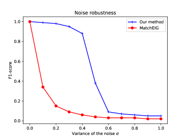
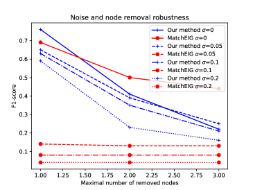
Figure 1: (left) The robustness of our method compare to MatchEIG following the variance of the noise. (right) The robustness of our method compare to MatchEIG following the maximal number of removed vertices and the variance of the noise.

Secondly, we assess the robustness of our method against vertex removal. For this, we remove vertices at random until a maximal number is reached. This means that for a given set of graphs, the number of vertices removed is not the same for all the graphs but cannot exceed the specified maximum. The removed vertices are disconnected from the other vertices and transformed into dummy in order to preserve an equal number of vertices. We also add different levels of noise on the attributes (same variance for edge and vertex data vectors). The results are presented by Figure 1(right). In absence of noise, MatchEIG shows a better robustness to vertex removal. But when we add the noise, our method performs better. Note that the matching quality degrades severely with increased maximal number of removed vertices. This is expected since removing vertices leads to changes in the edges and but also in the topology of the graphs.

4.2 Willow data-set

Willow is an image data-set composed of 5 classes of objects. For each class we have a minimum of 40 graphs with exactly 10 vertices. Here we use the same edge attributes as in Bernard et al. (2019) where the weights are computed using the median distance between vertices.

In order to find an appropriate set of hyper-parameters we run a grid-search on the variance for the Gaussian kernel on the vertices and the parameter of the RFF. The tested values range from $10$ to $100$ for an additive step of $10$ for the vertices and from $10^{-6}$ to $1$ with a multiplicative step of $0.1$ for the edges. For each set of values, we take at random 10 graphs from the car class and apply our method to estimate the F1-score. We repeat the process 10 times and report the mean of the scores. We use the set with the best mean score ($80$ for vertices and $10^{-5}$ for edges).

Method/Class	Car	Duck	Face	Motorbike	Winebottle
MatchEIG (Maset et al., 2017)	23.4	36.1	47.6	19.4	21.1
HiPPI (Bernard et al., 2019)	74.0	88.0	100	84.0	95.0
GA-MGM (Wang et al., 2020a)	74.6	90.0	99.7	89.2	93.7
Floyd-c (Jiang et al., 2020)	85.0	79.3	100	84.3	93.1
DGMC (Fey et al., 2020)	95.53	93.0	100	99.4	99.39
NGM-v2 (Wang et al., 2021)	97.4	93.4	100	98.6	98.3
Our (MatchEIG)	89.6	80.1	100	82.0	93.0
Our (GPow)	90.3	78.6	100	80.7	96.1
Our (IRGCL)	83.5	74.5	100	83.7	93.8

Table 1: F1-score of the different approaches on the Willow data-set. DGMC and NGM-v2 are supervised method where the vertices attributes are learned using deep learning framework. The others methods are unsupervised. We remind that the IRGCL method is combined with SQAD and initialized with MatchEIG result.

We present the results in Table 1. Here we use three methods for the projection onto permutations set: MatchEIG, GPow and IRGCL (with SQAD for the inner optimization step). For all methods expect MatchEIG we report the score from the articles. For MatchEIG we used our own implementation. The results show that we are competitive compared to other state-of-art methods. On the projection side, IRGCL leads to better results on motorbike while GPow is better on winebottle. Between the three methods, MatchEIG gives the best average results and is a little better than unsupervised state-of-art methods like Floyd-c (Jiang et al., 2020).

4.3 PascalVOC data-set

PascalVOC is an image data-set composed of 20 classes of objects with key points on each image. This database is challenging since the number of vertices vary greatly inside a class and there are also outliers. The number of vertices for a graph can vary from 1 to 16. For this data-set with follow the protocol from Fey et al. (2020) (it differs from the protocol of Wang et al. (2021) as they have different limits for the number of vertices). For comparison purpose we only use the test sets of each category.

Method/Class	Aero	Bike	Bird	Boat	Bottle	Bus	Car	Cat	Chair	Cow
MatchEIG (Maset et al., 2017)	9.0	15.3	15.8	16.8	19.8	23.5	13.3	13.0	11.5	9.4
NGM (unsup) (Wang et al., 2021)	30.8	42.5	44.3	33.8	39.8	52.2	49.2	53.9	27.5	42.4
SIGMA (Liu et al., 2021b)	55.1	70.6	57.8	71.3	88.0	88.6	88.2	75.5	46.8	70.9
DGMC (Fey et al., 2020)	50.1	65.4	55.7	65.3	80.0	83.5	78.3	69.7	34.7	60.7
NGM-v2 (Wang et al., 2021)	61.8	71.2	77.6	78.8	87.3	93.6	87.7	79.8	55.4	77.8
Ours (Eig)	10.7	41.6	24.6	24.3	47.6	31.0	19.0	24.1	14.4	10.4
Method/Class	Table	Dog	Horse	M-Bike	Person	Plant	Sheep	Sofa	Train	TV
MatchEIG (Maset et al., 2017)	19.2	12.2	9.6	11.7	6.5	20.1	10.6	15.3	28.0	36.5
NGM (unsup) (Wang et al., 2021)	29.3	49.1	45.1	45.1	24.0	48.3	49.9	29.9	70.2	73.3
SIGMA (Liu et al., 2021b)	90.4	66.5	78.0	67.5	65.0	96.7	68.5	97.9	94.3	86.1
DGMC (Fey et al., 2020)	70.4	59.9	70.0	62.2	56.1	80.2	70.3	88.8	81.1	84.3
NGM-v2 (Wang et al., 2021)	89.5	78.8	80.1	79.2	62.6	97.7	77.7	75.7	96.7	93.2
Ours (Eig)	15.4	15.1	15.4	20.3	8.0	60.2	10.6	17.2	48.3	62.3

Table 2: F1-score of the different approaches on the PascalVOC data-set.

For the hyper-parameters estimations we use the same protocol as for Willow (Section 4.2) but using the horse class. The optimal parameter were $60$ for vertices and $0.01$ for edges. We report the results in Table 2. Except MatchEIG where we use our own implementation, the results of the other methods are taken from the articles. Notice that we also report the results from NGM-v2 using an unsupervised setting with the same VGG16 data of the vertices. While supervised methods clearly perform better on this set, we are competitive with the two unsupervised methods. For computational reasons we did not apply IRGCL or GPow for the projection step. Interestingly while our method generally outperform MatchEIG, there are some classes where it is the reverse (e.g. tables). This could be explained by the way the edges are built (Delaunay tessellation). For some classes we are even better than the unsupervised version of NGM-v2 (bottle and plant).

These results are in line with our experiment on the robustness in Section 4.1. Since PascalVOC graphs are affected by noise and vertex suppression, our method performs badly on the most degraded category. Furthermore some categories are only composed by few graphs, for the test set. The cycle consistency is then insufficient to recover the good matches.

5 Conclusion and future work

We propose a generalization of the KerGM approach (Zhang et al., 2019) for multi-graph matching. Our approach allows for more flexibility than previous methods for dealing attributes on edges. While others methods directly deals with Lawler’s QAP, our approach relies on more efficient matrices and arrays and can be applied to larger and more complex data-sets. Contrary to other methods (Bernard et al., 2019; Wang et al., 2020a), we do not optimize in the universe of vertices, but directly manage the projection onto the permutation sets. This avoids some common limitations induced by the definition of the universe of vertices. In addition, our approach benefits from recently published methods to estimate the projection in reasonable computational times.

The kernel framework is very flexible and allows for specific definitions of the affinity on vertices and edges. For the edges we only use the classical Random Fourier Feature, but one can use more adapted features (Li et al., 2019) while keeping a tractable memory load. As an unsupervised method, the matching relies essentially on the constraints and the experiments show it is sufficient to deal with mild level of noise and almost homogeneous, in term of number of vertices, sets of graphs. Managing more complex sets requires either supervised learning or additional constraints.

Potential improvements include building a stochastic version of the method in order to be able to handle very large sets of graphs, for example by adapting stochastic DC methods (Xu et al., 2019). We also seek to improve the projection step while keeping an acceptable computational burden.

This work received support from the French government under the France 2030 investment plan, as part of the Initiative d’Excellence d’Aix-Marseille Université - A*MIDEX.

References

- Aflalo et al. (2015) Yonathan Aflalo, Alexander Bronstein, and Ron Kimmel. On convex relaxation of graph isomorphism. Proceedings of the National Academy of Sciences, 112(10):2942–2947, 2015.
- Bernard et al. (2019) Florian Bernard, Johan Thunberg, Paul Swoboda, and Christian Theobalt. HiPPI: Higher-order projected power iterations for scalable multi-matching. In Proceedings of the IEEE/CVF International Conference on Computer Vision, pages 10284–10293, 2019.
- Bernard et al. (2021) Florian Bernard, Daniel Cremers, and Johan Thunberg. Sparse quadratic optimisation over the Stiefel manifold with application to permutation synchronisation. Advances in Neural Information Processing Systems, 34, 2021.