Make Sharpness-Aware Minimization Stronger:
A Sparsified Perturbation Approach

Abstract

Deep neural networks often suffer from poor generalization caused by complex and non-convex loss landscapes. One of the popular solutions is Sharpness-Aware Minimization (SAM), which smooths the loss landscape via minimizing the maximized change of training loss when adding a perturbation to the weight. However, we find the indiscriminate perturbation of SAM on all parameters is suboptimal, which also results in excessive computation, i.e., double the overhead of common optimizers like Stochastic Gradient Descent (SGD). In this paper, we propose an efficient and effective training scheme coined as Sparse SAM (SSAM), which achieves sparse perturbation by a binary mask. To obtain the sparse mask, we provide two solutions which are based onFisher information and dynamic sparse training, respectively. In addition, we theoretically prove that SSAM can converge at the same rate as SAM, i.e., $O(\log T/\sqrt{T})$. Sparse SAM not only has the potential for training acceleration but also smooths the loss landscape effectively. Extensive experimental results on CIFAR10, CIFAR100, and ImageNet-1K confirm the superior efficiency of our method to SAM, and the performance is preserved or even better with a perturbation of merely 50% sparsity. Code is available at https://github.com/Mi-Peng/Sparse-Sharpness-Aware-Minimization.

1 Introduction

Over the past decade or so, the great success of deep learning has been due in great part to ever-larger model parameter sizes [13, 57, 53, 10, 40, 5]. However, the excessive parameters also make the model inclined to poor generalization. To overcome this problem, numerous efforts have been devoted to training algorithm [24, 42, 51], data augmentation [11, 58, 56], and network design [26, 28].

One important finding in recent research is the connection between the geometry of loss landscape and model generalization [31, 17, 27, 44, 54]. In general, the loss landscape of the model is complex and non-convex, which makes model tend to converge to sharp minima. Recent endeavors [31, 27, 44] show that the flatter the minima of convergence, the better the model generalization. This discovery reveals the nature of previous approaches [24, 26, 11, 56, 58, 28] to improve generalization, i.e., smoothing the loss landscape.

Based on this finding, Foret et al. [17] propose a novel approach to improve model generalization called sharpness-aware minimization (SAM), which simultaneously minimizes loss value and loss sharpness. SAM quantifies the landscape sharpness as the maximized difference of loss when a perturbation is added to the weight. When the model reaches a sharp area, the perturbed gradients in SAM help the model jump out of the sharp minima. In practice, SAM requires two forward-backward computations for each optimization step, where the first computation is to obtain the perturbation and the second one is for parameter update. Despite the remarkable performance [17, 34, 14, 7], This property makes SAM double the computational cost of the conventional optimizer, e.g., SGD [3].

Since SAM calculates perturbations indiscriminately for all parameters, a question is arisen:

Do we need to calculate perturbations for all parameters?

Above all, we notice that in most deep neural networks, only about 5% of parameters are sharp and rise steeply during optimization [31]. Then we explore the effect of SAM in different dimensions to answer the above question and find out (i) little difference between SGD and SAM gradients in most dimensions (see Fig. LABEL:fig:grad-diff); (ii) more flatter without SAM in some dimensions (see Fig. 4 and Fig. 5).

Inspired by the above discoveries, we propose a novel scheme to improve the efficiency of SAM via sparse perturbation, termed Sparse SAM (SSAM). SSAM, which plays the role of regularization, has better generalization, and its sparse operation also ensures the efficiency of optimization. Specifically, the perturbation in SSAM is multiplied by a binary sparse mask to determine which parameters should be perturbed. To obtain the sparse mask, we provide two implementations. The first solution is to use Fisher information [16] of the parameters to formulate the binary mask, dubbed SSAM-F. The other one is to employ dynamic sparse training to jointly optimize model parameters and the sparse mask, dubbed SSAM-D. The first solution is relatively more stable but a bit time-consuming, while the latter is more efficient.

In addition to these solutions, we provide the theoretical convergence analysis of SAM and SSAM in non-convex stochastic setting, proving that our SSAM can converge at the same rate as SAM, i.e., $O(\log T/\sqrt{T})$. At last, we evaluate the performance and effectiveness of SSAM on CIFAR10 [33], CIFAR100 [33] and ImageNet [8] with various models. The experiments confirm that SSAM contributes to a flatter landscape than SAM, and its performance is on par with or even better than SAM with only about 50% perturbation. These results coincide with our motivations and findings.

To sum up, the contribution of this paper is three-fold:

• We rethink the role of perturbation in SAM and find that the indiscriminate perturbations are suboptimal and computationally inefficient.

• We propose a sparsified perturbation approach called Sparse SAM (SSAM) with two variants, i.e., Fisher SSAM (SSAM-F) and Dynamic SSAM (SSAM-D), both of which enjoy better efficiency and effectiveness than SAM. We also theoretically prove that SSAM can converge at the same rate as SAM, i.e., $O(\log T/\sqrt{T})$.

• We evaluate SSAM with various models on CIFAR and ImageNet, showing WideResNet with SSAM of a high sparsity outperforms SAM on CIFAR; SSAM can achieve competitive performance with a high sparsity; SSAM has a comparable convergence rate to SAM.

2 Related Work

In this section, we briefly review the studies on sharpness-aware minimum optimization (SAM), Fisher information in deep learning, and dynamic sparse training.

SAM and flat minima. Hochreiter et al. [27] first reveal that there is a strong correlation between the generalization of a model and the flat minima. After that, there is a growing amount of research based on this finding. Keskar et al. [31] conduct experiments with a larger batch size, and in consequence observe the degradation of model generalization capability. They [31] also confirm the essence of this phenomenon, which is that the model tends to converge to the sharp minima. Keskar et al. [31] and Dinh et al. [12] state that the sharpness can be evaluated by the eigenvalues of the Hessian. However, they fail to find the flat minima due to the notorious computational cost of Hessian.

Inspired by this, Foret et al. [17] introduce a sharpness-aware optimization (SAM) to find a flat minimum for improving generalization capability, which is achieved by solving a mini-max problem. Zhang et al. [59] make a point that SAM [17] is equivalent to adding the regularization of the gradient norm by approximating Hessian matrix. Kwon et al. [34] propose a scale-invariant SAM scheme with adaptive radius to improve training stability. Zhang et al. [60] redefine the landscape sharpness from an intuitive and theoretical perspective based on SAM. To reduce the computational cost in SAM, Du et al. [14] proposed Efficient SAM (ESAM) to randomly calculate perturbation. However, ESAM randomly select the samples every steps, which may lead to optimization bias. Instead of the perturbations for all parameters, i.e., SAM, we compute a sparse perturbation, i.e., SSAM, which learns important but sparse dimensions for perturbation.

Fisher information (FI). Fisher information [16] was proposed to measure the information that an observable random variable carries about an unknown parameter of a distribution. In machine learning, Fisher information is widely used to measure the importance of the model parameters [32] and decide which parameter to be pruned [50, 52]. For proposed SSAM-F, Fisher information is used to determine whether a weight should be perturbed for flat minima.

Dynamic sparse training. Finding the sparse network via pruning unimportant weights is a popular solution in network compression, which can be traced back to decades [35]. The widely used training scheme, i.e., pretraining-pruning-fine-tuning, is presented by Han et.al. [23]. Limited by the requirement for the pre-trained model, some recent research [15, 2, 9, 30, 43, 37, 38] attempts to discover a sparse network directly from the training process. Dynamic Sparse Training (DST) finds the sparse structure by dynamic parameter reallocation. The criterion of pruning could be weight magnitude [18], gradient [15] and Hessian [35, 49], etc. We claim that different from the existing DST methods that prune neurons, our target is to obtain a binary mask for sparse perturbation.

3 Rethinking the Perturbation in SAM

In this section, we first review how SAM converges at the flat minimum of a loss landscape. Then, we rethink the role of perturbation in SAM.

3.1 Preliminary

In this paper, we consider the weights of a deep neural network as $\boldsymbol{w}=(w_{1},w_{2},...,w_{d})\subseteq\mathcal{W}\in\mathbb{R}^{d}$ and denote a binary mask as $\boldsymbol{m}\in\{0,1\}^{d}$, which satisfies $\boldsymbol{1}^{T}\boldsymbol{m}=(1-s)\cdot d$ to restrict the computational cost. Given a training dataset as $\mathcal{S}\triangleq\{(\boldsymbol{x}_{i},\boldsymbol{y}_{i})\}_{i=1}^{n}$ i.i.d. drawn from the distribution $\mathcal{D}$, the per-data-point loss function is defined by $f(\boldsymbol{w},\boldsymbol{x}_{i},\boldsymbol{y}_{i})$. For the classification task in this paper, we use cross-entropy as loss function. The population loss is defined by $f_{\mathcal{D}}=\mathbb{E}_{(\boldsymbol{x}_{i},\boldsymbol{y}_{i})\sim\mathcal{D}}f(\boldsymbol{w},\boldsymbol{x}_{i},\boldsymbol{y}_{i})$, while the empirical training loss function is $f_{\mathcal{S}}\triangleq\frac{1}{n}\sum_{i=1}^{n}f(\boldsymbol{w},\boldsymbol{x}_{i},\boldsymbol{y}_{i})$.

Sharpness-aware minimization (SAM) [17] aims to simultaneously minimize the loss value and smooth the loss landscape, which is achieved by solving the min-max problem:

$$\min_{\boldsymbol{w}}\max_{||\boldsymbol{\epsilon}||_{2}\leq\rho}f_{\mathcal{S}}(\boldsymbol{w}+\boldsymbol{\epsilon}).$$ (1)

SAM first obtains the perturbation $\boldsymbol{\epsilon}$ in a neighborhood ball area with a radius denoted as $\rho$. The optimization tries to minimize the loss of the perturbed weight $\boldsymbol{w}+\boldsymbol{\epsilon}$. Intuitively, the goal of SAM is that small perturbations to the weight will not significantly rise the empirical loss, which indicates that SAM tends to converge to a flat minimum. To solve the mini-max optimization, SAM approximately calculates the perturbations $\boldsymbol{\epsilon}$ using Taylor expansion around $\boldsymbol{w}$:

$$\boldsymbol{\epsilon}=\mathop{\arg\max}_{||\boldsymbol{\epsilon}||_{2}\leq\rho}f_{\mathcal{S}}(\boldsymbol{w}+\boldsymbol{\epsilon})\approx\mathop{\arg\max}_{||\boldsymbol{\epsilon}||_{2}\leq\rho}f_{\mathcal{S}}(\boldsymbol{w})+\boldsymbol{\epsilon}\cdot\nabla_{\boldsymbol{w}}f(\boldsymbol{w})=\rho\cdot{\nabla_{\boldsymbol{w}}f(\boldsymbol{w})}{\big{/}}{||\nabla_{\boldsymbol{w}}f(\boldsymbol{w})||_{2}}.$$ (2)

In this way, the objective function can be rewritten as $\min_{\boldsymbol{w}}f_{\mathcal{S}}\big{(}\boldsymbol{w}+\rho{\nabla_{\boldsymbol{w}}f(\boldsymbol{w})}{\big{/}}{||\nabla_{\boldsymbol{w}}f(\boldsymbol{w})||_{2}}\big{)}$, which could be implemented by a two-step gradient descent framework in Pytorch or TensorFlow:

• In the first step, the gradient at $\boldsymbol{w}$ is used to calculate the perturbation $\boldsymbol{\epsilon}$ by Eq. 2. Then the weight of model will be added to $\boldsymbol{w}+\boldsymbol{\epsilon}$.

• In the second step, the gradient at $\boldsymbol{w}+\boldsymbol{\epsilon}$ is used to solve $\min_{\boldsymbol{w}}f_{\mathcal{S}}(w+\boldsymbol{\epsilon})$, i.e., update the weight $\boldsymbol{w}$ by this gradient.

3.2 Rethinking the Perturbation Step of SAM

How does SAM work in flat subspace? SAM perturbs all parameters indiscriminately, but the fact is that merely about 5% parameter space is sharp while the rest is flat [31]. We are curious whether perturbing the parameters in those already flat dimensions would lead to the instability of the optimization and impair the improvement of generalization. To answer this question, we quantitatively and qualitatively analyze the loss landscapes with different training schemes in Section 5, as shown in  Fig. 4 and Fig. 5. The results confirm our conjecture that optimizing some dimensions without perturbation can help the model generalize better.

What is the difference between the gradients of SGD and SAM? We investigate various neural networks optimized with SAM and SGD on CIFAR10/100 and ImageNet, whose statistics are given in LABEL:fig:grad-diff. We use the relative difference ratio $r$, defined as $r=\log\left|{(g_{SAM}-g_{SGD})}/{g_{SGD}}\right|$, to measure the difference between the gradients of SAM and SGD. As showin in LABEL:fig:grad-diff, the parameters with $r$ less than 0 account for the vast majority of all parameters, indicating that most SAM gradients are not significantly different from SGD gradients. These results show that most parameters of the model require no perturbations for achieving the flat minima, which well confirms our the motivation.

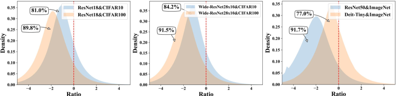
Figure 1: The distribution of relative difference ratio $r$ among various models and datasets. There is little difference between SAM and SGD gradients for most parameters, i.e., the ratio $r$ is less than $0$.

figure]fig:grad-diff

Inspired by the above observation and the promising hardware acceleration for sparse operation modern GPUs, we further propose Sparse SAM, a novel sparse perturbation approach, as an implicit regularization to improve the efficiency and effectiveness of SAM.

4 Methodology

In this section, we first define the proposed Sparse SAM (SSAM), which strengths SAM via sparse perturbation. Afterwards, we introduce the instantiations of the sparse mask used in SSAM via Fisher information and dynamic sparse training, dubbed SSAM-F and SSAM-D, respectively.

4.1 Sparse SAM

Motivated by the finding discussed in the introduction, Sparse SAM (SSAM) employs a sparse binary mask to decide which parameters should be perturbed, thereby improving the efficiency of sharpness-aware minimization. Specifically, the perturbation $\boldsymbol{\epsilon}$ will be multiplied by a sparse binary mask $\boldsymbol{m}$, and the objective function is then rewritten as $\min_{\boldsymbol{w}}f_{\mathcal{S}}\left(\boldsymbol{w}+\rho\cdot\frac{\nabla_{\boldsymbol{w}}f(\boldsymbol{w})}{||\nabla_{\boldsymbol{w}}f(\boldsymbol{w})||_{2}}\odot\boldsymbol{m}\right)$. To stable the optimization, the sparse binary mask $\boldsymbol{m}$ is updated at regular intervals during training. We provide two solutions to obtain the sparse mask $\boldsymbol{m}$, namely Fisher information based Sparse SAM (SSAM-F) and dynamic sparse training based Sparse SAM (SSAM-D). The overall algorithms of SSAM and sparse mask generations are shown in Algorithm 1 and Algorithm 2, respectively.

Algorithm 1 Sparse SAM (SSAM) 0:  sparse ratio $s$, dense model $\boldsymbol{w}$, binary mask $\boldsymbol{m}$, update interval $T_{m}$, number of samples $N_{F}$, learning rate $\eta$, training set $\mathcal{S}$. 1:  Initialize $\boldsymbol{w}$ and $\boldsymbol{m}$ randomly. 2:  for epoch $t=1,2\ldots T$ do 3:     for each training iteration do 4:        Sample a batch from $\mathcal{S}$: $\mathcal{B}$ 5:        Compute perturbation $\boldsymbol{\epsilon}$ by Eq. (2) 6:        if $t\mod T_{m}=0$ then 7:           Generate mask $m$ via Option I or II 8:        end if 9:        $\boldsymbol{\epsilon}\leftarrow\boldsymbol{\epsilon}\odot\boldsymbol{m}$ 10:     end for 11:     $\boldsymbol{w}\leftarrow\boldsymbol{w}-\eta\nabla f(\boldsymbol{w}+\boldsymbol{\epsilon})$ 12:  end for 13:  return  Final weight of model $\boldsymbol{w}$

Algorithm 2 Sparse Mask Generation 1:  Option I:(Fisher Information Mask) 2:  Sample $N_{F}$ data from $\mathcal{S}$: $\mathcal{B}_{F}$ 3:  Compute Fisher $\hat{F}_{\boldsymbol{w}}$ by Eq. (5) 4:  $\boldsymbol{m_{1}}\!=\!\{m_{i}\!=\!1|m_{i}\!\in\!\boldsymbol{m}\}\leftarrow{\rm ArgTopK}(\hat{F}_{\boldsymbol{w}},s\cdot|\boldsymbol{w}|)$ 5:  $\boldsymbol{m_{0}}\!=\!\{m_{i}\!=\!0|m_{i}\!\in\!\boldsymbol{m}\}\leftarrow\{m_{i}|m_{i}\!\notin\!\boldsymbol{m_{1}}\}$ 6:  $\boldsymbol{m}\leftarrow\boldsymbol{m_{0}}\cup\boldsymbol{m_{1}}$ 7:  Option II:(Dynamic Sparse Mask) 8:  $N_{drop}=f_{decay}(t;\alpha)\cdot(1-s)\cdot|\boldsymbol{w}|$ 9:  $N_{growth}=N_{drop}$ 10:  $\boldsymbol{m_{1}}\!=\!\{m_{i}\!=\!1|m_{i}\!\in\!\boldsymbol{m}\}\!\leftarrow\!\{m_{i}\!=\!1|m_{i}\!\in\!\boldsymbol{m}\}\!-\!{\rm ArgTopK}_{m_{i}\!\in\!\boldsymbol{m_{1}}}(-|\nabla f(\boldsymbol{w})|,N_{drop})$ 11:  $\boldsymbol{m_{1}}\!\leftarrow\!\{m_{i}\!=\!1|m_{i}\!\in\!\boldsymbol{m}\}+{\rm Random}_{\boldsymbol{m}_{i}\!\notin\!\boldsymbol{m_{1}}}(N_{growth})$ 12:  $\boldsymbol{m_{0}}\!=\!\{m_{i}\!=\!0|m_{i}\!\in\!\boldsymbol{m}\}\leftarrow\{m_{i}|m_{i}\!\notin\!\boldsymbol{m_{1}}\}$ 13:  $\boldsymbol{m}\leftarrow\boldsymbol{m_{0}}\cup\boldsymbol{m_{1}}$ 14:  return  Sparse mask $\boldsymbol{m}$

According to the previous work [55] and Ampere architecture equipped with sparse tensor cores [47, 46, 45], currently there exists technical support for matrix multiplication with 50% fine-grained sparsity [55]. Therefore, SSAM of 50% sparse perturbation has great potential to achieve true training acceleration via sparse back-propagation.

4.2 SSAM-F: Fisher information based Sparse SAM

Inspired by the connection between Fisher information and Hessian [16], which can directly measure the flatness of the loss landscape, we apply Fisher information to achieve sparse perturbation, denoted as SSAM-F. The Fisher information is defined by

$$F_{\boldsymbol{w}}=\mathbb{E}_{x\sim p(x)}\left[\mathbb{E}_{y\sim p_{\boldsymbol{w}}(y|x)}\nabla_{\boldsymbol{w}}\log p_{\boldsymbol{w}}(y|x)\nabla_{\boldsymbol{w}}\log p_{\boldsymbol{w}}(y|x)^{T}\right],$$ (3)

where $p_{\boldsymbol{w}}(y|x)$ is the output distribution predicted by the model. In over-parameterized networks, the computation of Fisher information matrix is also intractable, i.e., $|\boldsymbol{w}|\times|\boldsymbol{w}|$. Following [50, 19, 41, 22], we approximate $F_{\boldsymbol{w}}$ as a diagonal matrix, which is included in a vector in $\mathbb{R}^{|\boldsymbol{w}|}$. Note that there are the two expectation in Eq. (3). The first one is that the original data distribution $p(x)$ is often not available. Therefore, we approximate it by sampling $N_{F}$ data $\boldsymbol{x}_{1},\boldsymbol{x}_{2},\ldots,\boldsymbol{x}_{N_{F}}$ from $x\sim p(x)$:

$$F_{\boldsymbol{w}}=\frac{1}{N_{F}}\mathbb{E}_{y\sim p_{\boldsymbol{w}}(y|\boldsymbol{x}_{i})}(\nabla_{\boldsymbol{w}}\log p_{\boldsymbol{w}}(y|\boldsymbol{x}_{i}))^{2}.$$ (4)

For the second expectation over $p_{\boldsymbol{w}}(y|\boldsymbol{x})$, it is not necessary to compute its explicit expectation, since the ground-truth $y_{i}$ for each training sample $x_{i}$ is available in supervised learning. Therefore we rewrite the Eq. (4) as "empirical Fisher":

$$\hat{F}_{\boldsymbol{w}}=\frac{1}{N_{F}}(\nabla_{\boldsymbol{w}}\log p_{\boldsymbol{w}}(y_{i}|\boldsymbol{x}_{i}))^{2}.$$ (5)

We emphasize that the empirical Fisher is a $|\boldsymbol{w}|$-dimension vector, which is the same as the mask $\boldsymbol{m}$. To obtain the mask $\boldsymbol{m}$, we calculate the empirical Fisher by Eq. (5) over $N_{F}$ training data randomly sampled from training set $\mathcal{S}$. Then we sort the elements of empirical Fisher in descending, and the parameters corresponding to the the top $k$ Fisher values will be perturbed:

$$\boldsymbol{m_{1}}\!=\!\{m_{i}\!=\!1|m_{i}\!\in\!\boldsymbol{m}\}\leftarrow{\rm ArgTopK}(\hat{F}_{\boldsymbol{w}},k),$$ (6)

where ${\rm ArgTopK}(\boldsymbol{v},N)$ returns the index of the top $N$ largest values among $\boldsymbol{v}$, $\boldsymbol{m_{1}}$ is the set of values that are 1 in $\boldsymbol{m}$. $k$ is the number of perturbed parameters, which is equal to $(1-s)\cdot|\boldsymbol{w}|$ for sparsity $s$. After setting the rest values of the mask to 0, i.e., $\boldsymbol{m_{0}}=\{m_{i}=0|m_{i}\notin\boldsymbol{m_{1}}\}$, we get the final mask $\boldsymbol{m}=\boldsymbol{m_{0}}\cup\boldsymbol{m_{1}}$. The algorithm of SSAM-F is shown in Algorithm 2.

4.3 SSAM-D: Dynamic sparse training mask based sparse SAM

Considering the computation of empirical Fisher is still relatively high, we also resort to dynamic sparse training for efficient binary mask generation. The mask generation includes the perturbation dropping and the perturbation growth steps. At the perturbation dropping phase, the flattest dimensions of the perturbed parameters will be dropped, i.e., the gradients of lower absolute values, which means that they require no perturbations. The update of the sparse mask follows

$$\boldsymbol{m_{1}}=\{m_{i}=1|m_{i}\in\boldsymbol{m}\}\leftarrow\boldsymbol{m_{1}}-{\rm ArgTopK}_{\boldsymbol{w}\in\boldsymbol{m_{1}}}(-|\nabla f(\boldsymbol{w})|,N_{drop}),$$ (7)

where $N_{drop}$ is the number of perturbations to be dropped. At the perturbation growth phase, for the purpose of exploring the perturbation combinations as many as possible, several unperturbed dimensions grow, which means these dimensions need to compute perturbations. The update of the sparse mask for perturbation growth follows

$$\boldsymbol{m_{1}}=\{m_{i}=1|m_{i}\in\boldsymbol{m}\}\leftarrow\boldsymbol{m_{1}}+{\rm Random}_{\boldsymbol{w}\notin\boldsymbol{m_{1}}}(N_{growth}),$$ (8)

where ${\rm Random}_{\mathcal{S}}(N)$ randomly returns $N$ indexes in $\mathcal{S}$, and $N_{growth}$ is the number of perturbation growths. To keep the sparsity constant during training, the number of growths is equal to the number of dropping, i.e., $N_{growth}=N_{drop}$. Afterwards, we set the rest values of the mask to $0$, i.e., $\boldsymbol{m_{0}}\!=\!\{m_{i}\!=\!0|m_{i}\!\notin\!\boldsymbol{m_{1}}\}$, and get the final mask $\boldsymbol{m}\!=\!\boldsymbol{m_{0}}\cup\boldsymbol{m_{1}}$. The drop ratio $\alpha$ represents the proportion of dropped perturbations in the total perturbations $s\cdot|\boldsymbol{w}|$, i.e., $\alpha=N_{drop}/(s\cdot|\boldsymbol{w}|)$. In particular, a larger drop rate means that more combinations of binary mask can be explored during optimization, which, however, may slightly interfere the optimization process. Following [15, 9], we apply a cosine decay scheduler to alleviate this problem:

$$f_{decay}(t;\alpha)=\frac{\alpha}{2}\left(1+\cos\left({t\pi}{/}{T}\right)\right),$$ (9)

where $T$ denotes number of training epochs. The algorithm of SSAM-D is depicted in  Algorithm 2.

4.4 Theoretical analysis of Sparse SAM

In the following, we analyze the convergence of SAM and SSAM in non-convex stochastic setting. Before introducing the main theorem, we first describe the following assumptions that are commonly used for characterizing the convergence of nonconvex stochastic optimization [39, 60, 1, 6, 4, 20].

Assumption 1.

(Bounded Gradient.) It exists $G\geq 0$ s.t. $||\nabla f(\boldsymbol{w})||\leq G$.

Assumption 2.

(Bounded Variance.) It exists $\sigma\geq 0$ s.t. $\mathbb{E}[||g(\boldsymbol{w})-\nabla f(\boldsymbol{w})||^{2}]\leq\sigma^{2}$.

Assumption 3.

(L-smoothness.) It exists $L>0$ s.t. $||\nabla f(\boldsymbol{w})-\nabla f(\boldsymbol{v})||\leq L||\boldsymbol{w}-\boldsymbol{v}||$, $\forall\boldsymbol{w},\boldsymbol{v}\in\mathbb{R}^{d}$.

Theorem 1.

Consider function $f(\boldsymbol{w})$ satisfying the Assumptions 1-3 optimized by SAM. Let $\eta_{t}=\frac{\eta_{0}}{\sqrt{t}}$ and perturbation amplitude $\rho$ decay with square root of $t$, e.g., $\rho_{t}=\frac{\rho_{0}}{\sqrt{t}}$. With $\rho_{0}\leq G\eta_{0}$, we have

$$\frac{1}{T}\sum_{t=0}^{T}\mathbb{E}||\nabla f(\boldsymbol{w}_{t})||^{2}\leq C_{1}\frac{1}{\sqrt{T}}+C_{2}\frac{\log T}{\sqrt{T}},$$ (10)

where $C_{1}=\frac{2}{\eta_{0}}(f(\boldsymbol{w}_{0})-\mathbb{E}f(\boldsymbol{w}_{T}))$ and $C_{2}=2(L\sigma^{2}\eta_{0}+LG\rho_{0})$.

Theorem 2.

Consider function $f(\boldsymbol{w})$ satisfying the Assumptions 1-3 optimized by SSAM. Let $\eta_{t}=\frac{\eta_{0}}{\sqrt{t}}$ and perturbation amplitude $\rho$ decay with square root of $t$, e.g., $\rho_{t}=\frac{\rho_{0}}{\sqrt{t}}$. With $\rho_{0}\leq G\eta_{0}/2$, we have:

$$\frac{1}{T}\sum_{t=0}^{T}\mathbb{E}||\nabla f(\boldsymbol{w}_{t})||^{2}\leq C_{3}\frac{1}{\sqrt{T}}+C_{4}\frac{\log T}{\sqrt{T}},$$ (11)

where $C_{3}=\frac{2}{\eta_{0}}(f(\boldsymbol{w}_{0})-\mathbb{E}f(\boldsymbol{w}_{T})+\eta_{0}L^{2}\rho^{2}(1+\eta_{0}L)\frac{\pi^{2}}{6})$ and $C_{4}=2(L\sigma^{2}\eta_{0}+LG\rho_{0})$.

For non-convex stochastic optimization, Theorems 1&2 imply that our SSAM could converge the same rate as SAM, i.e., $O(\log T/\sqrt{T})$. Detailed proofs of the two theorems are given in Appendix.

5 Experiments

In this section, we evaluate the effectiveness of SSAM through extensive experiments on CIFAR10, CIFAR100 [33] and ImageNet-1K [8]. The base models include ResNet [25] and WideResNet [57]. We report the main results on CIFAR datasets in Tables 1&2 and ImageNet-1K in LABEL:imagenet-experiments. Then, we visualize the landscapes and Hessian spectra to verify that the proposed SSAM can help the model generalize better. More experimental results are placed in Appendix due to page limit.

5.1 Implementation details

Datasets. We use CIFAR10/CIFAR100 [33] and ImageNet-1K [8] as the benchmarks of our method. Specifically, CIFAR10 and CIFAR100 have 50,000 images of 32$\times$32 resolution for training, while 10,000 images for test. ImageNet-1K [8] is the most widely used benchmark for image classification, which has 1,281,167 images of 1000 classes and 50,000 images for validation.

Hyper-parameter setting. For small resolution datasets, i.e., CIFAR10 and CIFAR100, we replace the first convolution layer in ResNet and WideResNet with the one of 3$\times$3 kernel size, 1 stride and 1 padding. The models on CIFAR10/CIFAR100 are trained with 128 batch size for 200 epochs. We apply the random crop, random horizontal flip, normalization and cutout [11] for data augmentation, and the initial learning rate is 0.05 with a cosine learning rate schedule. The momentum and weight decay of SGD are set to 0.9 and 5e-4, respectively. SAM and SSAM apply the same settings, except that weight decay is set to 0.001 [14]. We determine the perturbation magnitude $\rho$ from $\{0.01,0.02,0.05,0.1,0.2,0.5\}$ via grid search. In CIFAR10 and CIFAR100, we set $\rho$ as 0.1 and 0.2, respectively. For ImageNet-1K, we randomly resize and crop all images to a resolution of 224$\times$224, and apply random horizontal flip, normalization during training. We train ResNet with a batch size of 256, and adopt the cosine learning rate schedule with initial learning rate 0.1. The momentum and weight decay of SGD is set as 0.9 and 1e-4. SAM and SSAM use the same settings as above. The test images of both architectures are resized to 256$\times$256 and then centerly cropped to 224$\times$224. The perturbation magnitude $\rho$ is set to 0.07.

5.2 Experimental results

Results on CIFAR10/CIFAR100. We first evaluate our SSAM on CIFAR-10 and CIFAR100. The models we used are ResNet-18 [25] and WideResNet-28-10 [57]. The perturbation magnitude $\rho$ for SAM and SSAM are the same for a fair comparison. As shown in Table 1, ResNet18 with SSAM of 50% sparsity outperforms SAM of full perturbations. From Table 2, we can observe that the advantages of SSAM-F and SSAM-D on WideResNet28 are more significant, which achieve better performance than SAM with up to 95% sparsity. Note that the parameter size of WideResNet28 is much larger than that of ResNet-18, and CIFAR is often easy to overfit. In addition, even with very large sparsity, both SSAM-F and SSAM-D can still obtain competitive performance against SAM.

Table 1: Comparison between SGD, SAM and SSAM on CIFAR using ResNet-18

Model	Optimizer	Sparsity	CIFAR10	CIFAR100	FLOPs
ResNet18	SGD	/	96.07%	77.80%	1$\times$
	SAM	0%	96.83%	81.03%	2$\times$
	SSAM-F (Ours)	50%	96.81% (-0.02)	81.24% (+0.21)	1.65$\times$
		80%	96.64% (-0.19)	80.47% (-0.56)	1.44$\times$
		90%	96.75% (-0.08)	80.02% (-1.01)	1.36$\times$
		95%	96.66% (-0.17)	80.50% (-0.53)	1.33$\times$
		98%	96.55% (-0.28)	80.09% (-0.94)	1.31$\times$
		99%	96.52% (-0.31)	80.07% (-0.96)	1.30$\times$
	SSAM-D (Ours)	50%	96.87% (+0.04)	80.59% (-0.44)	1.65$\times$
		80%	96.76% (-0.07)	80.43% (-0.60)	1.44$\times$
		90%	96.67% (-0.16)	80.39% (-0.64)	1.36$\times$
		95%	96.56% (-0.27)	79.79% (-1.24)	1.33$\times$
		98%	96.61% (-0.22)	79.79% (-1.24)	1.31$\times$
		99%	96.59% (-0.24)	79.61% (-1.42)	1.30$\times$

Table 2: Comparsion between SGD, SAM and SSAM on CIFAR using WideResNet-28-10

Model	Optimizer	Sparsity	CIFAR10	CIFAR100	FLOPs
WideResNet28-10	SGD	/	97.11%	81.93%	1$\times$
	SAM	0%	97.48%	84.20%	2$\times$
	SSAM-F (Ours)	50%	97.71% (+0.23)	85.16% (+0.96)	1.65$\times$
		80%	97.67% (+0.19)	84.57% (+0.37)	1.44$\times$
		90%	97.47% (-0.01)	84.76% (+0.56)	1.36$\times$
		95%	97.42% (-0.06)	84.17% (-0.03)	1.33$\times$
		98%	97.32% (-0.16)	83.85% (-0.35)	1.31$\times$
		99%	97.59% (+0.11)	84.00% (-0.20)	1.30$\times$
	SSAM-D (Ours)	50%	97.70% (+0.22)	84.99% (+0.79)	1.65$\times$
		80%	97.72% (+0.24)	84.36% (+0.16)	1.44$\times$
		90%	97.53% (+0.05)	84.16% (-0.04)	1.36$\times$
		95%	97.52% (+0.04)	83.66% (-0.54)	1.33$\times$
		98%	97.30% (-0.18)	83.30% (-0.90)	1.31$\times$
		99%	97.27% (-0.25)	84.16% (-0.04)	1.30$\times$

Results on ImageNet.  LABEL:imagenet-experiments reports the result of SSAM-F and SSAM-D on the large-scale ImageNet-1K [8] dataset. The model we used is ResNet50 [25]. We can observe that SSAM-F and SSAM-D can maintain the performance with 50% sparsity. However, as sparsity ratio increases, SSAM-F will receive relatively obvious performance drops while SSAM-D is more robust.

Table 3: Comparsion between SGD, SAM and SSAM on ImageNet-1K using ResNet50.

table]imagenet-experiments Model Optimizer Sparsity ImageNet FLOPs ResNet50 SGD / 76.67% 1$\times$ SAM 0% 77.25% 2$\times$ SSAM-F (Ours) 50% 77.31%(+0.06) 1.65$\times$ 80% 76.81%(-0.44) 1.44$\times$ 90% 76.74%(-0.51) 1.36$\times$ SSAM-D (Ours) 50% 77.25%(-0.00) 1.65$\times$ 80% 77.00%(-0.25) 1.44$\times$ 90% 77.00%(-0.25) 1.36$\times$

Training curves. We visualize the training curves of SGD, SAM and SSAM in LABEL:fig:train-curve. The training curves of SGD are more jittery, while SAM is more stable. In SSAM, about half of gradient updates are the same as SGD, but its training curves are similar to those of SAM, suggesting the effectiveness.

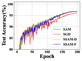
(a) ResNet18 on CIFAR10

(b) ResNet18 on CIFAR100

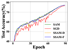
(c) ResNet50 on ImageNet-1K

Figure 2: The training curves of SGD, SAM and SSAM. The sparsity of SSAM is 50%.

figure]fig:train-curve

Sparsity vs. Accuracy. We report the effect of sparsity ratios in SSAM, as depicted in LABEL:fig:sparsity-acc. We can observe that on CIFAR datasets, the sparsities of SSAM-F and SSAM-D pose little impact on performance. In addition, they can obtain better accuracies than SAM with up to 99% sparsity. On the much larger dataset, i.e., ImageNet, a higher sparsity will lead to more obvious performance drop.

​​​

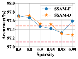
(a) WideResNet on CIFAR10.

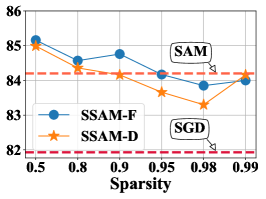
(b) WideResNet on CIFAR100.

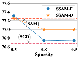
(c) ResNet50 on ImageNet.

Figure 3: Accuarcy v.s. sparsity on CIFAR10, CIFAR100 and ImageNet datasets.

figure]fig:sparsity-acc

5.3 SSAM with better generalization

Visualization of landscape. For a more intuitive comparison between different optimization schemes, we visualize the training loss landscapes of ResNet18 optimized by SGD, SAM and SSAM as shown in Fig. 4. Following [36], we sample $50\times 50$ points in the range of $[-1,1]$ from random "filter normalized" [36] directions, i.e., the $x$ and $y$ axes. As shown in Fig. 4, the landscape of SSAM is flatter than both SGD and SAM, and most of its area is low loss (blue). This result indicates that SSAM can smooth the loss landscape notably with sparse perturbation, and it also suggests that the complete perturbation on all parameters will result in suboptimal minima.

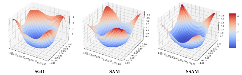
Figure 4: Training loss landscapes of ResNet18 on CIFAR10 trained with SGD, SAM, SSAM.

Hessian spectra. In Fig. 5, we report the Hessian spectrum to demonstrate that SSAM can converge to a flat minima. Here, we also report the ratio of dominant eigenvalue to fifth largest ones, i.e., $\lambda_{1}/\lambda_{5}$, used as the criteria in [17, 29]. We approximate the Hessian spectrum using the Lanczos algorithm [21] and illustrate the Hessian spectra of ResNet18 using SGD, SAM and SSAM on CIFAR10. From this figure, we observe that the dominant eigenvalue $\lambda_{1}$ with SSAM is less than SGD and comparable to SAM. It confirms that SSAM with a sparse perturbation can still converge to the flat minima as SAM does, or even better.

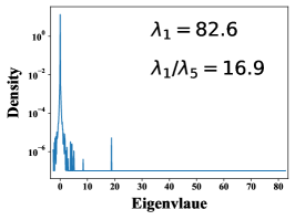
(a) SGD Hessian spectrum

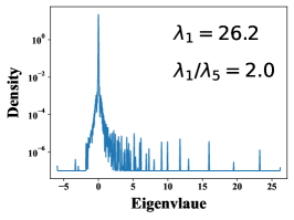
(b) SAM Hessian spectrum

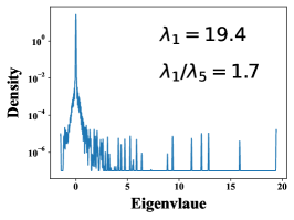
(c) SSAM Hessian spectrum

Figure 5: Hessian spectra of ResNet18 using SGD, SAM and SSAM on CIFAR10.

6 Conclusion

In this paper, we reveal that the SAM gradients for most parameters are not significantly different from the SGD ones. Based on this finding, we propose an efficient training scheme called Sparse SAM, which is achieved by computing a sparse perturbation. We provide two solutions for sparse perturbation, which are based on Fisher information and dynamic sparse training, respectively. In addition, we also theoretically prove that SSAM has the same convergence rate as SAM. We validate our SSAM on extensive datasets with various models. The experimental results show that retaining much better efficiency, SSAM can achieve competitive and even better performance than SAM.

Checklist

1. For all authors…

   1. Do the main claims made in the abstract and introduction accurately reflect the paper’s contributions and scope? [Yes]

   2. Did you describe the limitations of your work? [No]

   3. Did you discuss any potential negative societal impacts of your work? [No]

   4. Have you read the ethics review guidelines and ensured that your paper conforms to them? [Yes]

2. If you are including theoretical results…

   1. Did you state the full set of assumptions of all theoretical results? [Yes] See Section 4.4.

   2. Did you include complete proofs of all theoretical results? [Yes] The detailed proof is in Appendix.

3. If you ran experiments…

   1. Did you include the code, data, and instructions needed to reproduce the main experimental results (either in the supplemental material or as a URL)? [Yes]

   2. Did you specify all the training details (e.g., data splits, hyperparameters, how they were chosen)? [Yes] See Section 5.1.

   3. Did you report error bars (e.g., with respect to the random seed after running experiments multiple times)? [No]

   4. Did you include the total amount of compute and the type of resources used (e.g., type of GPUs, internal cluster, or cloud provider)? [No]

4. If you are using existing assets (e.g., code, data, models) or curating/releasing new assets…

   1. If your work uses existing assets, did you cite the creators? [N/A]

   2. Did you mention the license of the assets? [N/A]

   3. Did you include any new assets either in the supplemental material or as a URL? [N/A]

   4. Did you discuss whether and how consent was obtained from people whose data you’re using/curating? [N/A]

   5. Did you discuss whether the data you are using/curating contains personally identifiable information or offensive content? [N/A]

5. If you used crowdsourcing or conducted research with human subjects…

   1. Did you include the full text of instructions given to participants and screenshots, if applicable? [N/A]

   2. Did you describe any potential participant risks, with links to Institutional Review Board (IRB) approvals, if applicable? [N/A]

   3. Did you include the estimated hourly wage paid to participants and the total amount spent on participant compensation? [N/A]

Appendix A Missing Proofs

In this section, we will proof the main theorem in our paper. Before the detailed proof, we first recall the following assumptions that are commonly used for characterizing the convergence of non-convex stochastic optimization.

Assumption 1^′.

(Bounded Gradient.) It exists $G\geq 0$ s.t. $||\nabla f(\boldsymbol{w})||\leq G$.

Assumption 2^′.

(Bounded Variance.) It exists $\sigma\geq 0$ s.t. $\mathbb{E}[||g(\boldsymbol{w})-\nabla f(\boldsymbol{w})||^{2}]\leq\sigma^{2}$.

Assumption 3^′.

(L-smoothness.) It exists $L>0$ s.t. $||\nabla f(\boldsymbol{w})-\nabla f(\boldsymbol{v})||\leq L||\boldsymbol{w}-\boldsymbol{v}||$, $\forall\boldsymbol{w},\boldsymbol{v}\in\mathbb{R}^{d}$.

A.1 Proof of Theorem 1

Based on the objective function of Sharpness-Aware Minimization (SAM), suppose we can obtain the noisy observation gradient $g(\boldsymbol{w})$ of true gradient $\nabla f(\boldsymbol{w})$, we can write the iteration of SAM:

$$\left\{\begin{array}[]{ll}\boldsymbol{w}_{t+\frac{1}{2}}=&\boldsymbol{w}_{t}+\rho\cdot\frac{g(\boldsymbol{w}_{t})}{||g(\boldsymbol{w}_{t})||}\\ \boldsymbol{w}_{t+1}=&\boldsymbol{w}_{t}-\eta\cdot g(\boldsymbol{w}_{t+\frac{1}{2}})\end{array}\right.$$ (12)

Lemma 1.

For any $\rho>0$, $L>0$ and the differentiable function $f$, we have the following inequality:

$$\langle\nabla f(\boldsymbol{w}_{t}),\nabla f(\boldsymbol{w}_{t}+\rho\frac{\nabla f(\boldsymbol{w}_{t})}{||\nabla f(\boldsymbol{w}_{t})||})\rangle\geq||\nabla f(\boldsymbol{w}_{t})||^{2}-\rho LG$$

Proof.

We first add and subtract a term $||\nabla f(\boldsymbol{w}_{t})||$ to make use of classical inequalities bounding $\langle\nabla f(\boldsymbol{w}_{1})-\nabla f(\boldsymbol{w}_{2}),\boldsymbol{w}_{1}-\boldsymbol{w}_{2}\rangle$ by $||\boldsymbol{w}_{1}-\boldsymbol{w}_{2}||^{2}$ for smooth.

$$LHS= \langle\nabla f(\boldsymbol{w}_{t}),\nabla f(\boldsymbol{w}_{t}+\rho\frac{\nabla f(\boldsymbol{w}_{t})}{||\nabla f(\boldsymbol{w}_{t})||})-\nabla f(\boldsymbol{w}_{t})\rangle+||\nabla f(\boldsymbol{w}_{t})||^{2}$$

$$= \frac{||\nabla f(\boldsymbol{w}_{t})||}{\rho}\langle\frac{\rho}{||\nabla f(\boldsymbol{w}_{t})||}\nabla f(\boldsymbol{w}_{t}),\nabla f(\boldsymbol{w}_{t}+\rho\frac{\nabla f(\boldsymbol{w}_{t})}{||\nabla f(\boldsymbol{w}_{t})||}))-\nabla f(\boldsymbol{w}_{t})\rangle+||\nabla f(\boldsymbol{w}_{t})||^{2}$$

$$\geq -L\frac{||\nabla f(\boldsymbol{w}_{t})||}{\rho}||\frac{\rho}{||\nabla f(\boldsymbol{w}_{t})||}\nabla f(\boldsymbol{w}_{t})||^{2}+||\nabla f(\boldsymbol{w}_{t})||^{2}$$

$$= -||\nabla f(\boldsymbol{w}_{t})||\rho L+||\nabla f(\boldsymbol{w}_{t})||^{2}$$

$$\geq -G\rho L+||\nabla f(\boldsymbol{w}_{t})||^{2}$$

where the first inequality is that

$$\langle\nabla f(\boldsymbol{w}_{1})-\nabla f(\boldsymbol{w}_{2}),\boldsymbol{w}_{1}-\boldsymbol{w}_{2}\rangle\geq-L||\boldsymbol{w}_{1}-\boldsymbol{w}_{2}||^{2},$$

and the second inequality is the Assumption 1. ∎

Lemma 2.

For $\rho>0$, $L>0$, the iteration 12 satisfies following inequality:

$$\mathbb{E}\langle\nabla f(\boldsymbol{w}_{t}),g(\boldsymbol{w}_{t+\frac{1}{2}})\rangle\geq\frac{1}{2}||\nabla f(\boldsymbol{w}_{t})||^{2}-L^{2}\rho^{2}-L\rho G$$

Proof.

We denote the deterministic values of $\boldsymbol{w}_{t+\frac{1}{2}}$ as $\hat{\boldsymbol{w}}_{t+\frac{1}{2}}=\boldsymbol{w}_{t}+\rho\frac{\nabla f(\boldsymbol{w}_{t})}{||\nabla f(\boldsymbol{w}_{t})||}$ in this section. After we add and subtract the term $g(\hat{\boldsymbol{w}}_{t+\frac{1}{2}})$, we have the following equation:

$$\langle\nabla f(\boldsymbol{w}_{t}),g(\boldsymbol{w}_{t+\frac{1}{2}})\rangle= \langle\nabla f(\boldsymbol{w}_{t}),g(\boldsymbol{w}_{t}+\rho\frac{g(\boldsymbol{w}_{t})}{||g(\boldsymbol{w}_{t})||})-g(\hat{\boldsymbol{w}}_{t+\frac{1}{2}})\rangle+\langle g(\hat{\boldsymbol{w}}_{t+\frac{1}{2}}),\nabla f(\boldsymbol{w}_{t})\rangle$$

For the first term, we bound it by using the smoothness of $g(\boldsymbol{w})$:

$$-\langle\nabla f(\boldsymbol{w}_{t}),g(\boldsymbol{w}_{t}+\rho\frac{g(\boldsymbol{w}_{t})}{||g(\boldsymbol{w}_{t})||})-g(\hat{\boldsymbol{w}}_{t+\frac{1}{2}})\rangle\leq \frac{1}{2}||g(\boldsymbol{w}_{t}+\rho\frac{g(\boldsymbol{w}_{t})}{||g(\boldsymbol{w}_{t})||})-g(\hat{\boldsymbol{w}}_{t+\frac{1}{2}})||^{2}+\frac{1}{2}||\nabla f(\boldsymbol{w}_{t})||^{2}$$

$$\leq \frac{L^{2}}{2}||\boldsymbol{w}_{t}+\rho\frac{g(\boldsymbol{w}_{t})}{||g(\boldsymbol{w}_{t})||}-\hat{\boldsymbol{w}}_{t+\frac{1}{2}}||^{2}+\frac{1}{2}||\nabla f(\boldsymbol{w}_{t})||^{2}$$

$$= \frac{L^{2}}{2}||\boldsymbol{w}_{t}+\rho\frac{g(\boldsymbol{w}_{t})}{||g(\boldsymbol{w}_{t})||}-(\boldsymbol{w}_{t}+\rho\frac{\nabla f(\boldsymbol{w}_{t})}{||\nabla f(\boldsymbol{w}_{t})||})||^{2}+\frac{1}{2}||\nabla f(\boldsymbol{w}_{t})||^{2}$$

$$= \frac{L^{2}\rho^{2}}{2}||\frac{g(\boldsymbol{w}_{t})}{||g(\boldsymbol{w}_{t})||}-\frac{\nabla f(\boldsymbol{w}_{t})}{||\nabla f(\boldsymbol{w}_{t})||}||^{2}+\frac{1}{2}||\nabla f(\boldsymbol{w}_{t})||^{2}$$

$$\leq L^{2}\rho^{2}+\frac{1}{2}||\nabla f(\boldsymbol{w}_{t})||^{2}$$

For the second term, by using the Lemma 1, we have:

$$\mathbb{E}\langle g(\hat{\boldsymbol{w}}_{t+\frac{1}{2}}),\nabla f(\boldsymbol{w}_{t})\rangle= \langle\nabla f(\hat{\boldsymbol{w}}_{t+\frac{1}{2}}),\nabla f(\boldsymbol{w}_{t})\rangle$$

$$= \langle\nabla f(\boldsymbol{w}_{t}+\rho\frac{\nabla f(\boldsymbol{w}_{t})}{||\nabla f(\boldsymbol{w}_{t})||}),\nabla f(\boldsymbol{w}_{t})\rangle$$

$$\geq ||\nabla f(\boldsymbol{w}_{t})||^{2}-\rho LG$$

Asesmbling the two inequalities yields to the result. ∎

Lemma 3.

For $\eta\leq\frac{1}{L}$, the iteration 12 satisfies for all $t>0$:

$$\mathbb{E}f(\boldsymbol{w}_{t+1})\leq\mathbb{E}f(\boldsymbol{w}_{t})-\frac{\eta}{2}\mathbb{E}||\nabla f(\boldsymbol{w}_{t})||^{2}+L\eta^{2}\sigma^{2}+\eta L^{2}\rho^{2}+(1-L\eta)\eta LG\rho$$

Proof.

By the smoothness of the function $f$, we obtain

$$f(\boldsymbol{w}_{t+1})\leq f(\boldsymbol{w}_{t})-\eta\langle\nabla f(\boldsymbol{w}_{t}),g(\boldsymbol{w}_{t+\frac{1}{2}})\rangle+\frac{L\eta^{2}}{2}||g(\boldsymbol{w}_{t+\frac{1}{2}})||^{2}$$

$$= f(\boldsymbol{w}_{t})-\eta\langle\nabla f(\boldsymbol{w}_{t}),g(\boldsymbol{w}_{t+\frac{1}{2}})\rangle+\frac{L\eta^{2}}{2}(||\nabla f(\boldsymbol{w}_{t})-g(\boldsymbol{w}_{t+\frac{1}{2}})||^{2}-||\nabla f(\boldsymbol{w}_{t})||^{2}+2\langle\nabla f(\boldsymbol{w}_{t}),g(\boldsymbol{w}_{t+\frac{1}{2}})\rangle)$$

$$= f(\boldsymbol{w}_{t})-\frac{L\eta^{2}}{2}||\nabla f(\boldsymbol{w}_{t})||^{2}+\frac{L\eta^{2}}{2}||\nabla f(\boldsymbol{w}_{t})-g(\boldsymbol{w}_{t+\frac{1}{2}})||^{2}-(1-L\eta)\eta\langle\nabla f(\boldsymbol{w}_{t}),g(\boldsymbol{w}_{t+\frac{1}{2}})\rangle$$

$$\leq f(\boldsymbol{w}_{t})-\frac{L\eta^{2}}{2}||\nabla f(\boldsymbol{w}_{t})||^{2}+L\eta^{2}||\nabla f(\boldsymbol{w}_{t})-g(\boldsymbol{w}_{t})||^{2}+L\eta^{2}||g(\boldsymbol{w}_{t})-g(\boldsymbol{w}_{t+\frac{1}{2}})||^{2}$$

$$-(1-L\eta)\eta\langle\nabla f(\boldsymbol{w}_{t}),g(\boldsymbol{w}_{t+\frac{1}{2}})\rangle$$

$$\leq f(\boldsymbol{w}_{t})-\frac{L\eta^{2}}{2}||\nabla f(\boldsymbol{w}_{t})||^{2}+L\eta^{2}||\nabla f(\boldsymbol{w}_{t})-g(\boldsymbol{w}_{t})||^{2}+L\eta^{2}L^{2}||\boldsymbol{w}_{t}-\boldsymbol{w}_{t+\frac{1}{2}}||^{2}$$

$$-(1-L\eta)\eta\langle\nabla f(\boldsymbol{w}_{t}),g(\boldsymbol{w}_{t+\frac{1}{2}})\rangle$$

$$= f(\boldsymbol{w}_{t})-\frac{L\eta^{2}}{2}||\nabla f(\boldsymbol{w}_{t})||^{2}+L\eta^{2}||\nabla f(\boldsymbol{w}_{t})-g(\boldsymbol{w}_{t})||^{2}+\eta^{2}L^{3}\rho^{2}$$

$$-(1-L\eta)\eta\langle\nabla f(\boldsymbol{w}_{t}),g(\boldsymbol{w}_{t+\frac{1}{2}})\rangle$$

Taking the expectation and using Lemma 2 we obtain

$$\mathbb{E}f(\boldsymbol{w}_{t+1})\leq \mathbb{E}f(\boldsymbol{w}_{t})-\frac{L\eta^{2}}{2}\mathbb{E}||\nabla f(\boldsymbol{w}_{t})||^{2}+L\eta^{2}\mathbb{E}||\nabla f(\boldsymbol{w}_{t})-g(\boldsymbol{w}_{t})||^{2}+\eta^{2}L^{3}\rho^{2}$$

$$-(1-L\eta)\eta\mathbb{E}\langle\nabla f(\boldsymbol{w}_{t}),g(\boldsymbol{w}_{t+\frac{1}{2}})\rangle$$

$$\leq \mathbb{E}f(\boldsymbol{w}_{t})-\frac{L\eta^{2}}{2}\mathbb{E}||\nabla f(\boldsymbol{w}_{t})||^{2}+L\eta^{2}\sigma^{2}+\eta^{2}L^{3}\rho^{2}$$

$$-(1-L\eta)\eta\mathbb{E}\langle\nabla f(\boldsymbol{w}_{t}),g(\boldsymbol{w}_{t+\frac{1}{2}})\rangle$$

$$\leq \mathbb{E}f(\boldsymbol{w}_{t})-\frac{L\eta^{2}}{2}\mathbb{E}||\nabla f(\boldsymbol{w}_{t})||^{2}+L\eta^{2}\sigma^{2}+\eta^{2}L^{3}\rho^{2}$$

$$-(1-L\eta)\eta\left[\frac{1}{2}\mathbb{E}||\nabla f(\boldsymbol{w}_{t})||^{2}-L^{2}\rho^{2}-L\rho G\right]$$

$$= \mathbb{E}f(\boldsymbol{w}_{t})-\frac{\eta}{2}\mathbb{E}||\nabla f(\boldsymbol{w}_{t})||^{2}+L\eta^{2}\sigma^{2}+\eta^{2}L^{3}\rho^{2}+(1-L\eta)\eta L^{2}\rho^{2}+(1-L\eta)\eta L\rho G$$

$$= \mathbb{E}f(\boldsymbol{w}_{t})-\frac{\eta}{2}\mathbb{E}||\nabla f(\boldsymbol{w}_{t})||^{2}+L\eta^{2}\sigma^{2}+\eta L^{2}\rho^{2}+(1-L\eta)\eta LG\rho$$

∎

Proposition 1.

Let $\eta_{t}=\frac{\eta_{0}}{\sqrt{t}}$ and perturbation amplitude $\rho$ decay with square root of $t$, e.g., $\rho_{t}=\frac{\rho_{0}}{\sqrt{t}}$. For $\rho_{0}\leq G\eta_{0}$ and $\eta_{0}\leq\frac{1}{L}$, we have

$$\frac{1}{T}\sum_{t=1}^{T}\mathbb{E}||\nabla f(\boldsymbol{w}_{t})||^{2}\leq C_{1}\frac{1}{\sqrt{T}}+C_{2}\frac{\log T}{\sqrt{T}},$$

where $C_{1}=\frac{2}{\eta_{0}}(f(\boldsymbol{w}_{0})-\mathbb{E}f(\boldsymbol{w}_{T}))$ and $C_{2}=2(L\sigma^{2}\eta_{0}+LG\rho_{0})$.

Proof.

By Lemma 3, we replace $\rho$ and $\eta$ with $\rho_{t}=\frac{\rho_{0}}{\sqrt{t}}$ and $\eta_{t}=\frac{\eta_{0}}{\sqrt{t}}$, we have

$$\mathbb{E}f(\boldsymbol{w}_{t+1})\leq \mathbb{E}f(\boldsymbol{w}_{t})-\frac{\eta_{t}}{2}\mathbb{E}||\nabla f(\boldsymbol{w}_{t})||^{2}+L\eta_{t}^{2}\sigma^{2}+\eta_{t}L^{2}\rho_{t}^{2}+(1-L\eta_{t})\eta_{t}LG\rho_{t}.$$

Take telescope sum, we have

$$\mathbb{E}f(\boldsymbol{w}_{T})-f(\boldsymbol{w}_{0})\leq -\sum_{t=1}^{T}\frac{\eta_{t}}{2}\mathbb{E}||\nabla f(\boldsymbol{w}_{t})||^{2}+(L\sigma^{2}\eta_{0}^{2}+LG\rho_{0}\eta_{0})\sum_{t=1}^{T}\frac{1}{t}+(L^{2}\eta_{0}\rho_{0}^{2}-L^{2}G\eta_{0}^{2}\rho_{0})\sum_{t=1}^{T}\frac{1}{t^{\frac{3}{2}}}$$

Under $\rho_{0}\leq G\eta_{0}$, the last term will be less than 0, which means:

$$\mathbb{E}f(\boldsymbol{w}_{T})-f(\boldsymbol{w}_{0})\leq -\sum_{t=1}^{T}\frac{\eta_{t}}{2}\mathbb{E}||\nabla f(\boldsymbol{w}_{t})||^{2}+(L\sigma^{2}\eta_{0}^{2}+LG\rho_{0}\eta_{0})\sum_{t=1}^{T}\frac{1}{t}.$$

With

$$\frac{\eta_{T}}{2}\sum_{t=1}^{T}\mathbb{E}||\nabla f(\boldsymbol{w}_{t})||^{2}\leq \sum_{t=1}^{T}\frac{\eta_{t}}{2}\mathbb{E}||\nabla f(\boldsymbol{w}_{t})||^{2}\leq f(\boldsymbol{w}_{0})-\mathbb{E}f(\boldsymbol{w}_{T})+(L\sigma^{2}\eta_{0}^{2}+LG\rho_{0}\eta_{0})\sum_{t=1}^{T}\frac{1}{t},$$

we have

$$\frac{\eta_{0}}{2\sqrt{T}}\sum_{t=1}^{T}\mathbb{E}||\nabla f(\boldsymbol{w}_{t})||^{2}\leq f(\boldsymbol{w}_{0})-\mathbb{E}f(\boldsymbol{w}_{T})+(L\sigma^{2}\eta_{0}^{2}+LG\rho_{0}\eta_{0})\sum_{t=1}^{T}\frac{1}{t}$$

$$\leq f(\boldsymbol{w}_{0})-\mathbb{E}f(\boldsymbol{w}_{T})+(L\sigma^{2}\eta_{0}^{2}+LG\rho_{0}\eta_{0})\log T.$$

Finally, we achieve the result:

$$\frac{1}{T}\sum_{t=1}^{T}\mathbb{E}||\nabla f(\boldsymbol{w}_{t})||^{2}\leq \frac{2\cdot(f(\boldsymbol{w}_{0})-\mathbb{E}f(\boldsymbol{w}_{T}))}{\eta_{0}}\frac{1}{\sqrt{T}}+2(L\sigma^{2}\eta_{0}+LG\rho_{0})\frac{\log T}{\sqrt{T}},$$

which shows that SAM can converge at the rate of $O(\log T/\sqrt{T})$. ∎

A.2 Proof of Theorem 2

Suppose we can obtain the noisy observation gradient $g(\boldsymbol{w}_{t})$ of true gradient $\nabla f(\boldsymbol{w}_{t})$, and the mask $\boldsymbol{m}$, we can write the iteration of SAM: Consider the iteration of Sparse SAM:

$$\left\{\begin{array}[]{ll}\tilde{\boldsymbol{w}}_{t+\frac{1}{2}}=&\boldsymbol{w}_{t}+\rho\frac{g(\boldsymbol{w}_{t})}{||g(\boldsymbol{w}_{t})||}\odot\boldsymbol{m}_{t}\\ \boldsymbol{w}_{t+1}=&\boldsymbol{w}_{t}-g(\tilde{\boldsymbol{w}}_{t+\frac{1}{2}})\end{array}\right.$$ (15)

Let us denote the difference as $\boldsymbol{w}_{t+\frac{1}{2}}-\tilde{\boldsymbol{w}}_{t+\frac{1}{2}}=\boldsymbol{e}_{t}$.

Lemma 4.

With $\rho>0$, we have:

$$\mathbb{E}\langle\nabla f(\boldsymbol{w}_{t}),g(\tilde{\boldsymbol{w}}_{t+\frac{1}{2}})\rangle\geq\frac{1}{2}||\nabla f(\boldsymbol{w}_{t})||^{2}-2L^{2}\rho^{2}-L\rho G-L^{2}||\boldsymbol{e}_{t}||^{2}$$

Proof.

Similar to Lemma 2, We denote the true gradient as $\hat{\boldsymbol{w}}_{t+\frac{1}{2}}=\boldsymbol{w}_{t}+\rho\frac{\nabla f(\boldsymbol{w}_{t})}{||\nabla f(\boldsymbol{w}_{t})||}$, and also add and subtract the item $g(\tilde{\boldsymbol{w}}_{t+\frac{1}{2}})$:

$$\langle\nabla f(\boldsymbol{w}_{t}),g(\tilde{\boldsymbol{w}}_{t+\frac{1}{2}})\rangle= \langle\nabla f(\boldsymbol{w}_{t}),g(\tilde{\boldsymbol{w}}_{t+\frac{1}{2}})-g(\hat{\boldsymbol{w}}_{t+\frac{1}{2}})\rangle+\langle g(\hat{\boldsymbol{w}}_{t+\frac{1}{2}}),\nabla f(\boldsymbol{w}_{t})\rangle$$

For the first term, we bound it by using the smoothness of $g(\boldsymbol{w})$:

$$-\langle\nabla f(\boldsymbol{w}_{t}),g(\tilde{\boldsymbol{w}}_{t+\frac{1}{2}})-g(\hat{\boldsymbol{w}}_{t+\frac{1}{2}})\rangle\leq \frac{1}{2}||g(\tilde{\boldsymbol{w}}_{t+\frac{1}{2}})-g(\hat{\boldsymbol{w}}_{t+\frac{1}{2}})||^{2}+\frac{1}{2}||\nabla f(\boldsymbol{w}_{t})||^{2}$$

$$\leq \frac{L^{2}}{2}||\tilde{\boldsymbol{w}}_{t+\frac{1}{2}}-\hat{\boldsymbol{w}}_{t+\frac{1}{2}}||^{2}+\frac{1}{2}||\nabla f(\boldsymbol{w}_{t})||^{2}$$

$$= \frac{L^{2}}{2}||\boldsymbol{w}_{t+\frac{1}{2}}-\boldsymbol{e}_{t}-\hat{\boldsymbol{w}}_{t+\frac{1}{2}}||^{2}+\frac{1}{2}||\nabla f(\boldsymbol{w}_{t})||^{2}$$

$$\leq L^{2}(||\boldsymbol{w}_{t+\frac{1}{2}}-\hat{\boldsymbol{w}}_{t+\frac{1}{2}}||^{2}+||\boldsymbol{e}_{t}||^{2})+\frac{1}{2}||\nabla f(\boldsymbol{w}_{t})||^{2}$$

$$= L^{2}(\rho^{2}||\frac{g(\boldsymbol{w}_{t})}{||g(\boldsymbol{w}_{t})||}-\frac{\nabla f(\boldsymbol{w}_{t})}{||\nabla f(\boldsymbol{w}_{t})||}||^{2}+||\boldsymbol{e}_{t}||^{2})+\frac{1}{2}||\nabla f(\boldsymbol{w}_{t})||^{2}$$

$$\leq 2L^{2}\rho^{2}+L^{2}||\boldsymbol{e}_{t}||^{2}+\frac{1}{2}||\nabla f(\boldsymbol{w}_{t})||^{2}$$

For the second term, we do the same in Lemma 2:

$$\mathbb{E}\langle g(\hat{\boldsymbol{w}}_{t+\frac{1}{2}}),\nabla f(\boldsymbol{w}_{t})\rangle\geq ||\nabla f(\boldsymbol{w}_{t})||^{2}-\rho LG.$$

Assembling the two inequalities yields to the result. ∎

Lemma 5.

For $\eta\leq\frac{1}{L}$, the iteration 15 satisfies for all $t>0$:

$$\mathbb{E}f(\boldsymbol{w}_{t+1})\leq \mathbb{E}f(\boldsymbol{w}_{t})-\frac{\eta}{2}\mathbb{E}||\nabla f(\boldsymbol{w}_{t})||^{2}+L\eta^{2}\sigma^{2}+2\eta L^{2}\rho^{2}+(1-L\eta)\eta LG\rho$$

$$+(1+L\eta)\eta L^{2}||\boldsymbol{e}_{t}||^{2}$$

Proof.

By the smoothness of the function $f$, we obtain

$$f(\boldsymbol{w}_{t+1})\leq f(\boldsymbol{w}_{t})-\eta\langle\nabla f(\boldsymbol{w}_{t}),g(\tilde{\boldsymbol{w}}_{t+\frac{1}{2}})\rangle+\frac{L\eta^{2}}{2}||g(\tilde{\boldsymbol{w}}_{t+\frac{1}{2}})||^{2}$$

$$= f(\boldsymbol{w}_{t})-\eta\langle\nabla f(\boldsymbol{w}_{t}),g(\tilde{\boldsymbol{w}}_{t+\frac{1}{2}})\rangle+\frac{L\eta^{2}}{2}(||\nabla f(\boldsymbol{w}_{t})-g(\tilde{\boldsymbol{w}}_{t+\frac{1}{2}})||^{2}-||\nabla f(\boldsymbol{w}_{t})||^{2}+2\langle\nabla f(\boldsymbol{w}_{t}),g(\tilde{\boldsymbol{w}}_{t+\frac{1}{2}})\rangle)$$

$$= f(\boldsymbol{w}_{t})-\frac{L\eta^{2}}{2}||\nabla f(\boldsymbol{w}_{t})||^{2}+\frac{L\eta^{2}}{2}||\nabla f(\boldsymbol{w}_{t})-g(\tilde{\boldsymbol{w}}_{t+\frac{1}{2}})||^{2}-(1-L\eta)\eta\langle\nabla f(\boldsymbol{w}_{t}),g(\tilde{\boldsymbol{w}}_{t+\frac{1}{2}})\rangle$$

$$\leq f(\boldsymbol{w}_{t})-\frac{L\eta^{2}}{2}||\nabla f(\boldsymbol{w}_{t})||^{2}+L\eta^{2}||\nabla f(\boldsymbol{w}_{t})-g(\boldsymbol{w}_{t})||^{2}+L\eta^{2}||g(\boldsymbol{w}_{t})-g(\tilde{\boldsymbol{w}}_{t+\frac{1}{2}})||^{2}$$

$$-(1-L\eta)\eta\langle\nabla f(\boldsymbol{w}_{t}),g(\tilde{\boldsymbol{w}}_{t+\frac{1}{2}})\rangle$$

$$\leq f(\boldsymbol{w}_{t})-\frac{L\eta^{2}}{2}||\nabla f(\boldsymbol{w}_{t})||^{2}+L\eta^{2}||\nabla f(\boldsymbol{w}_{t})-g(\boldsymbol{w}_{t})||^{2}+L\eta^{2}L^{2}||\boldsymbol{w}_{t}-\tilde{\boldsymbol{w}}_{t+\frac{1}{2}}||^{2}$$

$$-(1-L\eta)\eta\langle\nabla f(\boldsymbol{w}_{t}),g(\tilde{\boldsymbol{w}}_{t+\frac{1}{2}})\rangle$$

$$= f(\boldsymbol{w}_{t})-\frac{L\eta^{2}}{2}||\nabla f(\boldsymbol{w}_{t})||^{2}+L\eta^{2}||\nabla f(\boldsymbol{w}_{t})-g(\boldsymbol{w}_{t})||^{2}+\eta^{2}L^{3}||\boldsymbol{w}_{t}-\boldsymbol{w}_{t+\frac{1}{2}}+\boldsymbol{e}_{t}||^{2}$$

$$-(1-L\eta)\eta\langle\nabla f(\boldsymbol{w}_{t}),g(\tilde{\boldsymbol{w}}_{t+\frac{1}{2}})\rangle$$

$$\leq f(\boldsymbol{w}_{t})-\frac{L\eta^{2}}{2}||\nabla f(\boldsymbol{w}_{t})||^{2}+L\eta^{2}||\nabla f(\boldsymbol{w}_{t})-g(\boldsymbol{w}_{t})||^{2}+2\eta^{2}L^{3}(||\boldsymbol{w}_{t}-\boldsymbol{w}_{t+\frac{1}{2}}||^{2}+||\boldsymbol{e}_{t}||^{2})$$

$$-(1-L\eta)\eta\langle\nabla f(\boldsymbol{w}_{t}),g(\tilde{\boldsymbol{w}}_{t+\frac{1}{2}})\rangle$$

$$= f(\boldsymbol{w}_{t})-\frac{L\eta^{2}}{2}||\nabla f(\boldsymbol{w}_{t})||^{2}+L\eta^{2}||\nabla f(\boldsymbol{w}_{t})-g(\boldsymbol{w}_{t})||^{2}+2\eta^{2}L^{3}(\rho^{2}+||\boldsymbol{e}_{t}||^{2})$$

$$-(1-L\eta)\eta\langle\nabla f(\boldsymbol{w}_{t}),g(\tilde{\boldsymbol{w}}_{t+\frac{1}{2}})\rangle$$

Taking the expectation and using Lemma 4 we obtain

$$\mathbb{E}f(\boldsymbol{w}_{t+1})\leq \mathbb{E}f(\boldsymbol{w}_{t})-\frac{L\eta^{2}}{2}\mathbb{E}||\nabla f(\boldsymbol{w}_{t})||^{2}+L\eta^{2}\mathbb{E}||\nabla f(\boldsymbol{w}_{t})-g(\boldsymbol{w}_{t})||^{2}+2\eta^{2}L^{3}(\rho^{2}+||\boldsymbol{e}_{t}||^{2})$$

$$-(1-L\eta)\eta\mathbb{E}\langle\nabla f(\boldsymbol{w}_{t}),g(\boldsymbol{w}_{t+\frac{1}{2}})\rangle$$

$$\leq \mathbb{E}f(\boldsymbol{w}_{t})-\frac{L\eta^{2}}{2}\mathbb{E}||\nabla f(\boldsymbol{w}_{t})||^{2}+L\eta^{2}\sigma^{2}+2\eta^{2}L^{3}(\rho^{2}+||\boldsymbol{e}_{t}||^{2})$$

$$-(1-L\eta)\eta\mathbb{E}\langle\nabla f(\boldsymbol{w}_{t}),g(\boldsymbol{w}_{t+\frac{1}{2}})\rangle$$

$$\leq \mathbb{E}f(\boldsymbol{w}_{t})-\frac{L\eta^{2}}{2}\mathbb{E}||\nabla f(\boldsymbol{w}_{t})||^{2}+L\eta^{2}\sigma^{2}+2\eta^{2}L^{3}(\rho^{2}+||\boldsymbol{e}_{t}||^{2})$$

$$-(1-L\eta)\eta\left[\frac{1}{2}||\nabla f(\boldsymbol{w}_{t})||^{2}-2L^{2}\rho^{2}-L\rho G-L^{2}||\boldsymbol{e}_{t}||^{2}\right]$$

$$= \mathbb{E}f(\boldsymbol{w}_{t})-\frac{\eta}{2}\mathbb{E}||\nabla f(\boldsymbol{w}_{t})||^{2}+L\eta^{2}\sigma^{2}+2\eta L^{2}\rho^{2}+(1-L\eta)\eta LG\rho$$

$$+(1+L\eta)\eta L^{2}||\rho\frac{g(\boldsymbol{w}_{t})}{||g(\boldsymbol{w}_{t})||}\odot\boldsymbol{m}_{t}-\rho\frac{g(\boldsymbol{w}_{t})}{||g(\boldsymbol{w}_{t})||}||^{2}$$

$$= \mathbb{E}f(\boldsymbol{w}_{t})-\frac{\eta}{2}\mathbb{E}||\nabla f(\boldsymbol{w}_{t})||^{2}+L\eta^{2}\sigma^{2}+2\eta L^{2}\rho^{2}+(1-L\eta)\eta LG\rho$$

$$+(1+L\eta)\eta L^{2}||\boldsymbol{e}_{t}||^{2}$$

∎

Proposition 2.

Let us $\eta_{t}=\frac{\eta_{0}}{\sqrt{t}}$ and perturbation amplitude $\rho$ decay with square root of $t$, e.g., $\rho_{t}=\frac{\rho_{0}}{\sqrt{t}}$. With $\rho_{0}\leq G\eta_{0}/2$, we have:

$$\frac{1}{T}\sum_{t=1}^{T}\mathbb{E}||\nabla f(\boldsymbol{w})||^{2}\leq C_{3}\frac{1}{\sqrt{T}}+C_{4}\frac{\log T}{\sqrt{T}},$$

where $C_{3}=\frac{2}{\eta_{0}}(f(\boldsymbol{w}_{0}-\mathbb{E}f(\boldsymbol{w}_{T})+\eta_{0}L^{2}\rho^{2}(1+\eta_{0}L)\frac{\pi^{2}}{6})$ and $C_{4}=2(L\sigma^{2}\eta_{0}+LG\rho_{0})$.

Proof.

By taking the expectation and using Lemma 4, and taking the schedule to be $\eta_{t}=\frac{\eta_{0}}{\sqrt{t}}$, $\rho_{t}=\frac{\rho_{0}}{\sqrt{t}}$, we obtain:

$$\mathbb{E}f(\boldsymbol{w}_{t+1})\leq \mathbb{E}f(\boldsymbol{w}_{t})-\frac{\eta_{t}}{2}\mathbb{E}||\nabla f(\boldsymbol{w}_{t})||^{2}+L\eta_{t}^{2}\sigma^{2}+2\eta_{t}L^{2}\rho_{t}^{2}+(1-L\eta_{t})\eta_{t}LG\rho_{t}$$

$$+(1+L\eta_{t})\eta_{t}L^{2}||\boldsymbol{e}_{t}||^{2}$$

By taking sum and bound $\rho$ with $\frac{G\eta_{0}}{2}$, we have:

$$\frac{\eta_{0}}{2\sqrt{T}}\sum_{t=1}^{T}\mathbb{E}||\nabla f(\boldsymbol{w}_{t})||^{2}\leq f(\boldsymbol{w}_{0})-\mathbb{E}f(\boldsymbol{w}_{T})+(L\sigma^{2}\eta_{0}^{2}+LG\rho_{0}\eta_{0})\sum_{t=1}^{T}\frac{1}{t}$$

$$+\sum_{t=1}^{T}(1+L\eta_{t})\eta_{t}L^{2}||\boldsymbol{e}_{t}||^{2}$$

$$\leq f(\boldsymbol{w}_{0})-\mathbb{E}f(\boldsymbol{w}_{T})+(L\sigma^{2}\eta_{0}^{2}+LG\rho_{0}\eta_{0})\sum_{t=1}^{T}\frac{1}{t}$$

$$+\eta_{0}L^{2}\rho_{0}^{2}\sum_{t=1}^{T}\frac{1}{t^{\frac{3}{2}}}+\eta_{0}^{2}L^{3}\rho^{2}\sum_{t=1}^{T}\frac{1}{t^{2}}$$

$$\leq f(\boldsymbol{w}_{0})-\mathbb{E}f(\boldsymbol{w}_{T})+(L\sigma^{2}\eta_{0}^{2}+LG\rho_{0}\eta_{0})\sum_{t=1}^{T}\frac{1}{t}$$

$$+\eta_{0}L^{2}\rho_{0}^{2}\sum_{t=1}^{T}\frac{1}{t^{2}}+\eta_{0}^{2}L^{3}\rho_{0}^{2}\sum_{t=1}^{T}\frac{1}{t^{2}}$$

$$\leq f(\boldsymbol{w}_{0})-\mathbb{E}f(\boldsymbol{w}_{T})+(L\sigma^{2}\eta_{0}^{2}+LG\rho_{0}\eta_{0})\log T$$

$$+\eta_{0}L^{2}\rho_{0}^{2}(1+\eta_{0}L)\frac{\pi^{2}}{6}$$

Finally, we achieve the result:

$$\frac{1}{T}\sum_{t=1}^{T}\mathbb{E}||\nabla f(\boldsymbol{w}_{t})||^{2}\leq \frac{2(f(\boldsymbol{w}_{0}-\mathbb{E}f(\boldsymbol{w}_{T})+\eta_{0}L^{2}\rho^{2}(1+\eta_{0}L)\frac{\pi^{2}}{6})}{\eta_{0}}\frac{1}{\sqrt{T}}$$

$$+2(L\sigma^{2}\eta_{0}+LG\rho_{0})\frac{\log T}{\sqrt{T}}$$

∎

So far, we have completed the proof of the theory in the main text.

Appendix B More Experimets

VGG on CIFAR10. To further confirm the model-agnostic characteristic of our Sparse SAM, we test the VGG-style architecture on CIFAR10. Following [48], we test SSAM training the VGG11-BN on CIFAR10 and the results are shown in the following LABEL:table:vgg-cifar-ssam. The perturbation magnitude $\rho$ is set to 0.05.

Table 4: Test accuracy of VGG11-BN on CIFAR10 with proposed Sparse SAM.

table]table:vgg-cifar-ssam Model Dataset Optimizer Sparsity Accuracy VGG11-BN CIFAR10 SGD / 93.42% SAM 0% 93.87% SSAM-F/SSAM-D 50% 94.03%/93.79% 80% 93.83%/93.95% 90% 93.76%/93.85% 95% 93.77%/93.48% 98% 93.54%/93.54% 99% 93.47%/93.33%

SAM with different perturbation magnitude $\rho$. We determine the perturbation magnitude $\rho$ by using grid search. We choose $\rho$ from the set $\{0.01,0.02,0.05,0.1,0.2,0.5\}$ for CIFAR, and choose $\rho$ from $\{0.01,0.02,0.05,0.07,0.1,0.2\}$ for ImageNet. We show the results when varying $\rho$ in LABEL:table:rho-cifar and Table 6. From this table, we can see that the $\rho=0.1$, $\rho=0.2$ and $\rho=0.07$ is sutiable for CIFAR10, CIFAR100 and ImageNet respectively.

Table 5: Test accuracy of ResNet18 and WideResNet28-10 on CIFAR10 and CIFAR100 with different perturbation magnitude $\rho$.

table]table:rho-cifar Dataset SAM $\rho$ 0.01 0.02 0.05 0.1 0.2 0.5 ResNet18 96.58% 96.54% 96.68% 96.83% 96.32% 93.16% CIFAR10 WideResNet28-10 97.26% 97.34% 97.31% 97.48% 97.29% 95.13% ResNet18 79.56% 79.98% 80.71% 80.65% 81.03% 77.57% CIFAR100 WideResNet28-10 82.25% 83.04% 83.47% 83.47% 84.20% 84.03%

Table 6: Test accuracy of ResNet50 on ImageNet with different perturbation magnitude $\rho$.

datasets	SAM $\rho$	0.01	0.02	0.05	0.07	0.1	0.2
ImageNet	ResNet50	76.63%	76.78%	77.12%	77.25%	77.00%	76.37%

Ablations of Masking Strategy. For further verification of our masking strategy, we perform more ablations in this paragraph. For the mask update in SSAM-F, the parameters with largest fisher information are selected. Compared with SSAM-F, we consider the random mask, i.e., the mask is randomly generated to choose which parameters are perturbated. For the mask update in SSAM-D, we first drop the flattest weights and then random grow some weights. Compared with SSAM-D, we experiment the SSAM-D which drops randomly or drops the sharpest weights, i.e., the weights with large gradients. The results of ablations are shown in LABEL:table:mask-strategy. The results show that random strategies are less effective than our SSAM. The performance of SSAM-D dropping sharpest weights drops a lot even worse than random strategy, which is consistent with our conjecture.

Table 7: Ablation of different masking strategy.

table]table:mask-strategy Model Dataset Optimizer Strategy Accuracy ResNet50 ImageNet SGD / 76.67% SAM / 77.25% Sparse SAM Random Mask 77.08%(-0.17) SSAM-F Topk Fisher Information 77.31%(+0.06) SSAM-D Random Drop 77.08%(-0.17) Drop Sharpnest weights 76.68%(-0.57) Drop Flattest weights 77.25%(-0.00)

Influence of hyper-parameters We first examine the effect of the number of sample size $N_{F}$ of SSAM-F in Table 9. From it we can see that a certain number of samples is enough for the approximation of data distribution in SSAM-F, e.g., $N_{F}=128$, which greatly saves the computational cost of SSAM-F. In Table 9, we also report the influence of the mask update interval on SSAM-F and SSAM-D. The results show that the performance degrades as the interval becom longer, suggesting that dense mask updates are necessary for our methods. Both of them are ResNet18 on CIFAR10.

Table 8: Results of ResNet18 on CIFAR10 with different number of samples $N_{F}$ in SSAM-F. ‘Time’ reported in table is the time cost to calculate Fisher Information based on $N_{F}$ samples.

Sparsity	$N_{F}$	Acc	Time
0.5	16	96.77%	1.49s
	128	96.84%	4.40s
	512	96.67%	15.35s
	1024	96.83%	30.99s
	2048	96.68%	56.23s
	4096	96.66%	109.31s
0.9	16	96.79%	1.47s
	128	96.50%	5.42s
	512	96.43%	15.57s
	1024	96.75%	29.24s
	2048	96.62%	57.72s
	4096	96.59%	110.65s

Table 9: Results of ResNet18 on CIFAR10 with different $T_{m}$ intervals of update mask. The left of ‘/’ is accuracy of SSAM-F, while the right is SSAM-D.

Sparsity	$T_{m}$	Acc
0.5	1	96.81%/96.74%
	2	96.51%/96.74%
	5	96.83%/96.60%
	10	96.71%/96.73%
	50	96.65%/96.75%
	Fixed	96.57%/96.52%
0.9	1	96.70%/96.65%
	2	93.75%/96.63%
	5	96.51%/96.69%
	10	96.67%/96.74%
	50	96.64%/96.66%
	Fixed	96.21%/96.46%

Appendix C Limitation and Societal Impacts

Limitation. Our method Sparse SAM is mainly based on sparse operation. At present, the sparse operation that has been implemented is only 2:4 sparse operation. The 2:4 sparse operation requires that there are at most two non-zero values in four contiguous memory, which does not hold for us. To sum up, there is currently no concrete implemented sparse operation to achieve training acceleration. But in the future, with the development of hardware for sparse operation, our method has great potential to achieve truly training acceleration.

Societal Impacts. In this paper, we provide a Sparse SAM algorithm that reduces computation burden and improves model generalization. In the future, we believe that with the development of deep learning, more and more models need the guarantee of generalization and also the efficient training. Different from the work on sparse networks, our proposed Sparse SAM does not compress the model for hardware limited device, but instead accelerates model training. It’s helpful for individuals or laboratories which are lack computing resources.

References

- Andriushchenko and Flammarion [2021] Maksym Andriushchenko and Nicolas Flammarion. Understanding sharpness-aware minimization. 2021.
- Bellec et al. [2017] Guillaume Bellec, David Kappel, Wolfgang Maass, and Robert Legenstein. Deep rewiring: Training very sparse deep networks. arXiv preprint arXiv:1711.05136, 2017.
- Bottou [2010] Léon Bottou. Large-scale machine learning with stochastic gradient descent. In Proceedings of COMPSTAT’2010, pages 177–186. Springer, 2010.
- Bottou et al. [2018] Léon Bottou, Frank E Curtis, and Jorge Nocedal. Optimization methods for large-scale machine learning. Siam Review, 60(2):223–311, 2018.
- Brock et al. [2018] Andrew Brock, Jeff Donahue, and Karen Simonyan. Large scale gan training for high fidelity natural image synthesis. arXiv preprint arXiv:1809.11096, 2018.
- Chen et al. [2022] Congliang Chen, Li Shen, Fangyu Zou, and Wei Liu. Towards practical adam: Non-convexity, convergence theory, and mini-batch acceleration. Journal of Machine Learning Research, 23:1–47, 2022.
- Chen et al. [2021] Xiangning Chen, Cho-Jui Hsieh, and Boqing Gong. When vision transformers outperform resnets without pre-training or strong data augmentations. arXiv preprint arXiv:2106.01548, 2021.
- Deng et al. [2009] Jia Deng, Wei Dong, Richard Socher, Li-Jia Li, Kai Li, and Li Fei-Fei. Imagenet: A large-scale hierarchical image database. In 2009 IEEE conference on computer vision and pattern recognition, pages 248–255. Ieee, 2009.
- Dettmers and Zettlemoyer [2019] Tim Dettmers and Luke Zettlemoyer. Sparse networks from scratch: Faster training without losing performance. arXiv preprint arXiv:1907.04840, 2019.
- Devlin et al. [2018] Jacob Devlin, Ming-Wei Chang, Kenton Lee, and Kristina Toutanova. Bert: Pre-training of deep bidirectional transformers for language understanding. arXiv preprint arXiv:1810.04805, 2018.
- DeVries and Taylor [2017] Terrance DeVries and Graham W Taylor. Improved regularization of convolutional neural networks with cutout. arXiv preprint arXiv:1708.04552, 2017.
- Dinh et al. [2017] Laurent Dinh, Razvan Pascanu, Samy Bengio, and Yoshua Bengio. Sharp minima can generalize for deep nets. In International Conference on Machine Learning, pages 1019–1028. PMLR, 2017.
- Dosovitskiy et al. [2020] Alexey Dosovitskiy, Lucas Beyer, Alexander Kolesnikov, Dirk Weissenborn, Xiaohua Zhai, Thomas Unterthiner, Mostafa Dehghani, Matthias Minderer, Georg Heigold, Sylvain Gelly, et al. An image is worth 16x16 words: Transformers for image recognition at scale. arXiv preprint arXiv:2010.11929, 2020.
- Du et al. [2021] Jiawei Du, Hanshu Yan, Jiashi Feng, Joey Tianyi Zhou, Liangli Zhen, Rick Siow Mong Goh, and Vincent YF Tan. Efficient sharpness-aware minimization for improved training of neural networks. arXiv preprint arXiv:2110.03141, 2021.
- Evci et al. [2020] Utku Evci, Trevor Gale, Jacob Menick, Pablo Samuel Castro, and Erich Elsen. Rigging the lottery: Making all tickets winners. In International Conference on Machine Learning, pages 2943–2952. PMLR, 2020.
- Fisher [1922] Ronald A Fisher. On the mathematical foundations of theoretical statistics. Philosophical transactions of the Royal Society of London. Series A, containing papers of a mathematical or physical character, 222(594-604):309–368, 1922.
- Foret et al. [2020] Pierre Foret, Ariel Kleiner, Hossein Mobahi, and Behnam Neyshabur. Sharpness-aware minimization for efficiently improving generalization. In International Conference on Learning Representations, 2020.
- Frankle and Carbin [2018] Jonathan Frankle and Michael Carbin. The lottery ticket hypothesis: Finding sparse, trainable neural networks. arXiv preprint arXiv:1803.03635, 2018.
- George et al. [2018] Thomas George, César Laurent, Xavier Bouthillier, Nicolas Ballas, and Pascal Vincent. Fast approximate natural gradient descent in a kronecker factored eigenbasis. Advances in Neural Information Processing Systems, 31, 2018.
- Ghadimi and Lan [2013] Saeed Ghadimi and Guanghui Lan. Stochastic first-and zeroth-order methods for nonconvex stochastic programming. SIAM Journal on Optimization, 23(4):2341–2368, 2013.
- Ghorbani et al. [2019] Behrooz Ghorbani, Shankar Krishnan, and Ying Xiao. An investigation into neural net optimization via hessian eigenvalue density. In International Conference on Machine Learning, pages 2232–2241. PMLR, 2019.
- Grosse and Martens [2016] Roger Grosse and James Martens. A kronecker-factored approximate fisher matrix for convolution layers. In International Conference on Machine Learning, pages 573–582. PMLR, 2016.
- Han et al. [2015] Song Han, Huizi Mao, and William J Dally. Deep compression: Compressing deep neural networks with pruning, trained quantization and huffman coding. arXiv preprint arXiv:1510.00149, 2015.
- Hansen et al. [1997] Lars Kai Hansen, Jan Larsen, and Torben Fog. Early stop criterion from the bootstrap ensemble. In 1997 IEEE International Conference on Acoustics, Speech, and Signal Processing, volume 4, pages 3205–3208. IEEE, 1997.
- He et al. [2016] Kaiming He, Xiangyu Zhang, Shaoqing Ren, and Jian Sun. Deep residual learning for image recognition. In Proceedings of the IEEE conference on computer vision and pattern recognition, pages 770–778, 2016.
- Hinton et al. [2012] Geoffrey E Hinton, Nitish Srivastava, Alex Krizhevsky, Ilya Sutskever, and Ruslan R Salakhutdinov. Improving neural networks by preventing co-adaptation of feature detectors. arXiv preprint arXiv:1207.0580, 2012.
- Hochreiter and Schmidhuber [1994] Sepp Hochreiter and Jürgen Schmidhuber. Simplifying neural nets by discovering flat minima. Advances in neural information processing systems, 7, 1994.
- Ioffe and Szegedy [2015] Sergey Ioffe and Christian Szegedy. Batch normalization: Accelerating deep network training by reducing internal covariate shift. In International conference on machine learning, pages 448–456. PMLR, 2015.
- Jastrzebski et al. [2020] Stanislaw Jastrzebski, Maciej Szymczak, Stanislav Fort, Devansh Arpit, Jacek Tabor, Kyunghyun Cho, and Krzysztof Geras. The break-even point on optimization trajectories of deep neural networks. arXiv preprint arXiv:2002.09572, 2020.
- Jayakumar et al. [2020] Siddhant Jayakumar, Razvan Pascanu, Jack Rae, Simon Osindero, and Erich Elsen. Top-kast: Top-k always sparse training. Advances in Neural Information Processing Systems, 33:20744–20754, 2020.
- Keskar et al. [2016] Nitish Shirish Keskar, Dheevatsa Mudigere, Jorge Nocedal, Mikhail Smelyanskiy, and Ping Tak Peter Tang. On large-batch training for deep learning: Generalization gap and sharp minima. 2016.
- Kirkpatrick et al. [2017] James Kirkpatrick, Razvan Pascanu, Neil Rabinowitz, Joel Veness, Guillaume Desjardins, Andrei A Rusu, Kieran Milan, John Quan, Tiago Ramalho, Agnieszka Grabska-Barwinska, et al. Overcoming catastrophic forgetting in neural networks. Proceedings of the national academy of sciences, 114(13):3521–3526, 2017.
- Krizhevsky et al. [2009] Alex Krizhevsky et al. Learning multiple layers of features from tiny images. 2009.
- Kwon et al. [2021] Jungmin Kwon, Jeongseop Kim, Hyunseo Park, and In Kwon Choi. Asam: Adaptive sharpness-aware minimization for scale-invariant learning of deep neural networks. In International Conference on Machine Learning, pages 5905–5914. PMLR, 2021.
- LeCun et al. [1989] Yann LeCun, John Denker, and Sara Solla. Optimal brain damage. Advances in neural information processing systems, 2, 1989.
- Li et al. [2018] Hao Li, Zheng Xu, Gavin Taylor, Christoph Studer, and Tom Goldstein. Visualizing the loss landscape of neural nets. Advances in neural information processing systems, 31, 2018.
- Liu et al. [2021a] Shiwei Liu, Tianlong Chen, Xiaohan Chen, Zahra Atashgahi, Lu Yin, Huanyu Kou, Li Shen, Mykola Pechenizkiy, Zhangyang Wang, and Decebal Constantin Mocanu. Sparse training via boosting pruning plasticity with neuroregeneration. Advances in Neural Information Processing Systems, 34:9908–9922, 2021a.
- Liu et al. [2021b] Shiwei Liu, Tianlong Chen, Xiaohan Chen, Li Shen, Decebal Constantin Mocanu, Zhangyang Wang, and Mykola Pechenizkiy. The unreasonable effectiveness of random pruning: Return of the most naive baseline for sparse training. In International Conference on Learning Representations, 2021b.
- Liu et al. [2021c] Yong Liu, Xiangning Chen, Minhao Cheng, Cho-Jui Hsieh, and Yang You. Concurrent adversarial learning for large-batch training. arXiv preprint arXiv:2106.00221, 2021c.
- Liu et al. [2021d] Ze Liu, Yutong Lin, Yue Cao, Han Hu, Yixuan Wei, Zheng Zhang, Stephen Lin, and Baining Guo. Swin transformer: Hierarchical vision transformer using shifted windows. In Proceedings of the IEEE/CVF International Conference on Computer Vision, pages 10012–10022, 2021d.
- Martens and Grosse [2015] James Martens and Roger Grosse. Optimizing neural networks with kronecker-factored approximate curvature. In International conference on machine learning, pages 2408–2417. PMLR, 2015.
- Mnih et al. [2016] Volodymyr Mnih, Adria Puigdomenech Badia, Mehdi Mirza, Alex Graves, Timothy Lillicrap, Tim Harley, David Silver, and Koray Kavukcuoglu. Asynchronous methods for deep reinforcement learning. In International conference on machine learning, pages 1928–1937. PMLR, 2016.
- Mostafa and Wang [2019] Hesham Mostafa and Xin Wang. Parameter efficient training of deep convolutional neural networks by dynamic sparse reparameterization. In International Conference on Machine Learning, pages 4646–4655. PMLR, 2019.
- Neyshabur et al. [2017] Behnam Neyshabur, Srinadh Bhojanapalli, David McAllester, and Nati Srebro. Exploring generalization in deep learning. Advances in neural information processing systems, 30, 2017.
- [45] nvidia ampere architecture. Nvidia ampere tensor core. https://www.nvidia.com/en-us/data-center/ampere-architecture/.
- [46] nvidia auto sparsity. Accelerating sparsity in the nvidia ampere architecture. https://developer.download.nvidia.com/video/gputechconf/gtc/2020/presentations/s22085-accelerating-sparsity-in-the-nvidia-ampere-architecture%E2%80%8B.pdf.
- [47] nvidia whitepaper. Nvidia a100 tensor core gpu architecture. https://images.nvidia.com/aem-dam/en-zz/Solutions/data-center/nvidia-ampere-architecture-whitepaper.pdf.
- Pytorch Cifar [100] Pytorch Cifar100. Pytorch cifar100 github. https://github.com/weiaicunzai/pytorch-cifar100.
- Singh and Alistarh [2020] Sidak Pal Singh and Dan Alistarh. Woodfisher: Efficient second-order approximation for neural network compression. Advances in Neural Information Processing Systems, 33:18098–18109, 2020.
- Sung et al. [2021] Yi-Lin Sung, Varun Nair, and Colin A Raffel. Training neural networks with fixed sparse masks. Advances in Neural Information Processing Systems, 34, 2021.
- Szegedy et al. [2016] Christian Szegedy, Vincent Vanhoucke, Sergey Ioffe, Jon Shlens, and Zbigniew Wojna. Rethinking the inception architecture for computer vision. In Proceedings of the IEEE conference on computer vision and pattern recognition, pages 2818–2826, 2016.
- Theis et al. [2018] Lucas Theis, Iryna Korshunova, Alykhan Tejani, and Ferenc Huszár. Faster gaze prediction with dense networks and fisher pruning. arXiv preprint arXiv:1801.05787, 2018.
- Vaswani et al. [2017] Ashish Vaswani, Noam Shazeer, Niki Parmar, Jakob Uszkoreit, Llion Jones, Aidan N Gomez, Łukasz Kaiser, and Illia Polosukhin. Attention is all you need. Advances in neural information processing systems, 30, 2017.
- Wu et al. [2020] Dongxian Wu, Shu-Tao Xia, and Yisen Wang. Adversarial weight perturbation helps robust generalization. Advances in Neural Information Processing Systems, 33:2958–2969, 2020.
- Xu et al. [2022] Weixiang Xu, Xiangyu He, Ke Cheng, Peisong Wang, and Jian Cheng. Towards fully sparse training: Information restoration with spatial similarity. 2022.
- Yun et al. [2019] Sangdoo Yun, Dongyoon Han, Seong Joon Oh, Sanghyuk Chun, Junsuk Choe, and Youngjoon Yoo. Cutmix: Regularization strategy to train strong classifiers with localizable features. In Proceedings of the IEEE/CVF international conference on computer vision, pages 6023–6032, 2019.
- Zagoruyko and Komodakis [2016] Sergey Zagoruyko and Nikos Komodakis. Wide residual networks. arXiv preprint arXiv:1605.07146, 2016.
- Zhang et al. [2017] Hongyi Zhang, Moustapha Cisse, Yann N Dauphin, and David Lopez-Paz. mixup: Beyond empirical risk minimization. arXiv preprint arXiv:1710.09412, 2017.
- Zhao et al. [2022] Yang Zhao, Hao Zhang, and Xiuyuan Hu. Penalizing gradient norm for efficiently improving generalization in deep learning. arXiv preprint arXiv:2202.03599, 2022.
- Zhuang et al. [2022] Juntang Zhuang, Boqing Gong, Liangzhe Yuan, Yin Cui, Hartwig Adam, Nicha Dvornek, Sekhar Tatikonda, James Duncan, and Ting Liu. Surrogate gap minimization improves sharpness-aware training. arXiv preprint arXiv:2203.08065, 2022.