LARF: Two-level Attention-based Random Forests with a Mixture of Contamination Models

Abstract

New models of the attention-based random forests called LARF (Leaf Attention-based Random Forest) are proposed. The first idea behind the models is to introduce a two-level attention, where one of the levels is the “leaf” attention and the attention mechanism is applied to every leaf of trees. The second level is the tree attention depending on the “leaf” attention. The second idea is to replace the softmax operation in the attention with the weighted sum of the softmax operations with different parameters. It is implemented by applying a mixture of the Huber’s contamination models and can be regarded as an analog of the multi-head attention with “heads” defined by selecting a value of the softmax parameter. Attention parameters are simply trained by solving the quadratic optimization problem. To simplify the tuning process of the models, it is proposed to make the tuning contamination parameters to be training and to compute them by solving the quadratic optimization problem. Many numerical experiments with real datasets are performed for studying LARFs. The code of proposed algorithms can be found in https://github.com/andruekonst/leaf-attention-forest.

Keywords: attention mechanism, random forest, Nadaraya-Watson regression, quadratic programming, contamination model

1 Introduction

Several crucial improvements of neural networks have been made in recent years. One of them is the attention mechanism which has played an important role in many machine learning areas, including the natural language processing models, the computer vision, etc. [1, 2, 3, 4, 5]. The idea behind the attention mechanism is to assign weights to features or examples in accordance with their importance and their impact on the model predictions. At the same time, the success of the attention models as components of neural network motivates to extend this approach to other machine learning models different from neural networks, for example, to random forests (RFs) [6]. Following this idea, a new model called the attention-based random forest (ABRF), which incorporates the attention mechanism into ensemble-based models such as RFs and the gradient boosting machine [7, 8] has been developed [9, 10]. The ABRF models stems from the interesting interpretation [1, 11] of the attention mechanism through the Nadaraya-Watson kernel regression model [12, 13]. According to [9, 10], attention weights in the Nadaraya-Watson regression are assigned to decision trees in a RF depending on examples which fall into leaves of trees. Weights in ABRF have trainable parameters and use the Huber’s $\epsilon$-contamination model [14] for defining the attention weights such that each attention weight consists of two parts: the softmax operation with the tuning coefficient $1-\epsilon$ and the trainable bias of the softmax weight with coefficient $\epsilon$. One of the improvements of ABRF, which has been proposed in [15], is based on joint incorporating self-attention and attention mechanisms into the RF. The proposed models outperform ABRF, but this outperformance is not sufficient. The model for several dataset provided inferior results. Therefore, we propose a set of models which can be regarded as extensions of ABRF and are based on two main ideas.

The first idea is to introduce a two-level attention, where one of the levels is the “leaf” attention, i.e., the attention mechanism is applied to every leaf of trees. As a result, we get the attention weights assigned to leaves and the attention weights assigned to trees. At that, the attention weights of trees depend on the corresponding weights of leaves belonging to these trees. In other words, the attention at the second level depends on the attention at the first level, i.e., we get the attention of the attention. Due to the “leaf” attention, the proposed model will be abbreviated as LARF (Leaf Attention-based Random Forest).

One of the peculiarities of LARFs is the use of a mixture of the Huber’s $\epsilon$-contamination models instead of the single contamination model as it has been done in ABRF. This peculiarity stems from the second idea behind the model to take into account the softmax operation with different parameters simultaneously. In fact, we replace the standard softmax operation by the weighted sum of the softmax operations with different parameters. With this idea, we achieve two goals. First of all, we partially solve the problem of tuning parameters of the softmax operations which are a part of attention operations. Each value of the tuning parameter from a predefined set (from a predefined grid) is used in a separate softmax operation. Then weights of the softmax operations in the sum are trained jointly with training other parameters. This approach can also be interpreted as the linear approximation of the softmax operations with trainable weights and with different values of tuning parameters. However, a more interesting goal is that some analog of the multi-head attention [16] is implemented by using the mixture of contamination models where “heads” are defined by selecting a value of the corresponding softmax operation parameter.

Additionally, in contrast to ABRF [10] where the contamination parameter $\epsilon$ of the Huber’s model was a tuning parameter, the LARF model considers this parameter as the training one. This allows us to significantly reduce the model tuning time and to avoid enumeration of the parameter values in accordance with a grid. The same is implemented for the mixture of the Huber’s models.

Different configurations of LARF produce a set of models which depend on trainable parameters of the two-level attention and its implementation.

We investigate two types of RFs in experiments: original RFs and Extremely Randomized Trees (ERT) [17]. According to [17], the ERT algorithm chooses a split point randomly for each feature at each node and then selects the best split among these.

Our contributions can be summarized as follows:

1. New two-level attention-based RF models are proposed, where the attention mechanism at the first level is applied to every leaf of trees, the attention at the second level incorporates the “leaf” attention and is applied to trees. Training of the two-level attention is reduced to solving the standard quadratic optimization problem.

2. A mixture of the Huber’s $\epsilon$-contamination models is used to implement the attention mechanism at the second level. The mixture allows us to replace a set of tuning attention parameters (the temperature parameters of the softmax operations) with trainable parameters whose optimal values are computed by solving the quadratic optimization problem. Moreover, this approach can be regarded as an analog of the multi-head attention.

3. An approach is proposed to make the tuning contamination parameters ($\epsilon$ parameters) in the mixture of the $\epsilon$-contamination models to be training. Their optimal values are also computed by solving the quadratic optimization problem.

4. Many numerical experiments with real datasets are performed for studying LARFs. They demonstrate outperforming results of some modifications of LARF. The code of proposed algorithms can be found in https://github.com/andruekonst/leaf-attention-forest.

The paper is organized as follows. Related work can be found in Section 2. A brief introduction to the attention mechanism as the Nadaraya-Watson kernel regression is given in Section 3. A general approach to incorporating the two-level attention mechanism into the RF is provided in Section 4. Ways for implementation of the two-level attention mechanism and constructing several attention-based models by using the mixture of the Huber’s $\epsilon$-contamination models are considered in Section 5. Numerical experiments with real data illustrating properties of the proposed models are provided in Section 6. Concluding remarks can be found in Section 7.

2 Related work

Attention mechanism. Due to the great efficiency of machine learning models with the attention mechanisms, interest in the different attention-based models has increased significantly in recent years. As a result, many attention models have been proposed to improve the performance of machine learning algorithms. The most comprehensive analysis and description of various attention-based models can be found in interesting surveys [1, 2, 3, 4, 5, 18].

It is important to note that parametric attention models as parts of neural networks are mainly trained by applying the gradient-based algorithms which lead to computational problems when training is carried out through the softmax function. Many approaches have been proposed to cope with this problem. A large part of approaches is based on some kinds of linear approximation of the softmax attention of [19, 20, 21, 22]. Another part of the approaches is based on random feature methods to approximate the softmax function [18, 23].

Another improvement of the attention-based models is to use the self-attention which was proposed in [16] as a crucial component of neural networks called Transformers. The self-attention models have been also studied in surveys [4, 24, 25, 26, 27, 28]. This is only a small part of all works devoted to the attention and self-attention mechanisms.

It should be noted that the aforementioned models are implemented as neural networks, and they have not been studied for application to other machine learning models, for example, to RFs. Attempts to incorporate the attention and self-attention mechanisms into the RF and the gradient boosting machine were made in [9, 10, 15]. Following these works, we extend the proposed models to improve the attention-based models. Moreover, we propose the attention models which do not use the gradient-based algorithms for computing optimal attention parameters. The training process of the models is based on solving standard quadratic optimization problems.

Weighted RFs. Many approaches have been proposed in recent years to improve RFs. One of the important approaches is based on assignment of weights to decision trees in the RF. This approach is implemented in various algorithms [29, 30, 31, 32, 33, 34, 35]. However, most these algorithms have an disadvantage. The weights are assigned to trees independently of examples, i.e., each weight characterizes trees on the average over all training examples and does not take into account any feature vector. Moreover, the weights do not have training parameters which usually make the model more flexible and accurate.

Contamination model in attention mechanisms. There are several models which use imprecise probabilities in order to model the lack of sufficient training data. One of the first models is the so-called Credal Decision Tree, which is based on applying the imprecise probability theory to classification and proposed in [36]. Following this work, a number of models based on imprecise probabilities were presented in [37, 38, 39, 40] where the imprecise Dirichlet model is used. This model can be regarded as a reparametrization of the imprecise $\epsilon$-contamination model which is applied to LARF. The imprecise $\epsilon$-contamination model has been also applied to machine learning methods, for example, to the support vector machine [41] or to the RF [42]. The attention-based RF applying the imprecise $\epsilon$-contamination model to the parametric attention mechanism was proposed in [10, 15]. However, there were no other works which use the imprecise models in order to implement the attention mechanism.

3 Nadaraya-Watson regression and the attention mechanism

A basis of the attention mechanism can be considered in the framework of the Nadaraya-Watson kernel regression model [12, 13] which estimates a function $f$ as a locally weighted average using a kernel as a weighting function. Suppose that the dataset is represented by $n$ examples $(\mathbf{x}_{1},y_{1}),...,(\mathbf{x}_{n},y_{n})$, where $\mathbf{x}_{i}=(x_{i1},...,x_{im})\in\mathbb{R}^{m}$ is a feature vector consisting of $m$ features; $y_{i}\in\mathbb{R}$ is a regression output. The regression task is to construct a regressor $f:\mathbb{R}^{m}\rightarrow\mathbb{R}$ which can predict the output value $\tilde{y}$ of a new observation $\mathbf{x}$, using the dataset.

The Nadaraya-Watson kernel regression estimates the regression output $\tilde{y}$ corresponding to a new input feature vector $\mathbf{x}$ as follows [12, 13]:

$$\tilde{y}=\sum_{i=1}^{n}\alpha(\mathbf{x},\mathbf{x}_{i})y_{i},$$ (1)

where weight $\alpha(\mathbf{x},\mathbf{x}_{i})$ conforms with relevance of the feature vector $\mathbf{x}_{i}$ to the vector $\mathbf{x}$.

It can be seen from the above that the Nadaraya-Watson regression model estimates $\tilde{y}$ as a weighted sum of training outputs $y_{i}$ from the dataset such that their weights depend on location of $\mathbf{x}_{i}$ relative to $\mathbf{x}$. This mean that the closer $\mathbf{x}_{i}$ to $\mathbf{x}$, the greater the weight assigned to $y_{i}$.

According to the Nadaraya-Watson kernel regression [12, 13], weights can be defined by means of a kernel $K$ as a function of the distance between vectors $\mathbf{x}_{i}$ and $\mathbf{x}$. The kernel estimates how $\mathbf{x}_{i}$ is close to $\mathbf{x}$. Then the weight is written as follows:

$$\alpha(\mathbf{x},\mathbf{x}_{i})=\frac{K(\mathbf{x},\mathbf{x}_{i})}{\sum_{j=1}^{n}K(\mathbf{x},\mathbf{x}_{j})}.$$ (2)

One of the popular kernel is the Gaussian kernel. It produces weights of the form:

$$\alpha(\mathbf{x},\mathbf{x}_{i})=\text{$\sigma$}\left(-\frac{\left\|\mathbf{x}-\mathbf{x}_{i}\right\|^{2}}{\tau}\right),$$ (3)

where $\tau$ is a tuning (temperature) parameter; $\sigma\left(\cdot\right)$ is a notation of the softmax operation.

In terms of the attention mechanism [43], vector $\mathbf{x}$, vectors $\mathbf{x}_{i}$, outputs $y_{i}$ and weight $\alpha(\mathbf{x},\mathbf{x}_{i})$ are called as the query, keys, values and the attention weight, respectively. Weights $\alpha(\mathbf{x},\mathbf{x}_{i})$ can be extended by incorporating trainable parameters. In particular, parameter $\tau$ can be also regarded as the trainable parameter.

Many forms of parametric attention weights, which also define the attention mechanisms, have been proposed, for example, the additive attention [43], the multiplicative or dot-product attention [16, 44]. We will consider also the attention weights based on the Gaussian kernels, i.e., producing the softmax operation. However, the parametric forms of the attention weights will be quite different from many popular attention operations.

4 Two-level attention-based random forest

One of the powerful machine learning models handling with tabular data is the RF which can be regarded as an ensemble of $T$ decision trees such that each tree is trained on a subset of examples randomly selected from the training set. In the original RF, the final RF prediction $\tilde{y}$ for a testing example $\mathbf{x}$ is determined by averaging predictions $\tilde{y}_{1},...,\tilde{y}_{T}$ obtained for all trees.

Let $\mathcal{J}_{k}(\mathbf{x})$ be the index set of examples which fall into the same leaf in the $k$-th tree as $\mathbf{x}$. One of the ways to construct the attention-based RF is to introduce the mean vector $\mathbf{A}_{k}(\mathbf{x)}$ defined as the mean of training vectors $\mathbf{x}_{j}$ which fall into the same leaf as $\mathbf{x}$. However, this simple definition can be extended by incorporating the Nadaraya-Watson regression into the leaf. In this case, we can write

$$\mathbf{A}_{k}(\mathbf{x)}=\sum_{j\in\mathcal{J}_{k}(\mathbf{x})}\mu\left(\mathbf{x},\mathbf{x}_{j}\right)\mathbf{x}_{j},$$ (4)

where $\mu\left(\mathbf{x},\mathbf{x}_{j}\right)$ is the attention weight in accordance with the Nadaraya-Watson kernel regression.

In fact, (4) can be regarded as the self-attention. The idea behind (4) is that we find the mean value of $\mathbf{x}$ by assigning weights to training examples which fall into the corresponding leaf in accordance with their vicinity to the vector $\mathbf{x}$.

In the same way, we can define the mean value of regression outputs corresponding to examples falling into the same leaf as $\mathbf{x}$:

$$B_{k}(\mathbf{x)}=\sum_{j\in\mathcal{J}_{k}(\mathbf{x})}\mu\left(\mathbf{x},\mathbf{x}_{j}\right)y_{j}.$$ (5)

Expression (5) can be regarded as the attention. The idea behind (5) is to get the prediction provided by the corresponding leaf by using the standard attention mechanism or the Nadaraya-Watson regression. In other words, we weigh predictions provided by the $k$-th leaf of a tree in accordance with the distance between the feature vector $\mathbf{x}$, which falls into the $k$-th leaf, and all feature vectors $\mathbf{x}_{j}$ which fall into the same leaf. It should be noted that the original regression tree provides the averaged prediction, i.e., it corresponds to the case when all $\mu\left(\mathbf{x},\mathbf{x}_{j}\right)$ are identical for all $j\in\mathcal{J}_{k}(\mathbf{x})$ and equal to $1/\#\mathcal{J}_{k}(\mathbf{x})$.

We suppose that the attention mechanisms used above are non-parametric. This implies that weights do not have trainable parameters. It is assumed that

$$\sum_{j\in\mathcal{J}_{k}(\mathbf{x})}\mu\left(\mathbf{x},\mathbf{x}_{j}\right)=1.$$ (6)

The “leaf” attention introduced above can be regarded as the first-level attention in a hierarchy of the attention mechanisms. It characterizes how the feature vector $\mathbf{x}$ fits the corresponding tree.

If we suppose that the whole RF consists of $T$ decision trees, then the set of $\mathbf{A}_{k}(\mathbf{x)}$, $k=1,...,T$, in the framework of the attention mechanism can be regarded as a set of keys for every $\mathbf{x}$, the set of $B_{k}(\mathbf{x)}$, $k=1,...,T$, can be regarded as a set of values. This implies that the final prediction $\tilde{y}$ of the RF can be computed by using the Nadaraya-Watson regression, namely,

$$\tilde{y}=f(\mathbf{x},\mathbf{w})=\sum_{k=1}^{T}\alpha\left(\mathbf{x},\mathbf{A}_{k}(\mathbf{x}),\mathbf{w}\right)B_{k}(\mathbf{x)}.$$ (7)

Here $\alpha\left(\mathbf{x},\mathbf{A}_{k}(\mathbf{x)},\mathbf{w}\right)$ is the attention weight with vector $\mathbf{w}=(w_{1},...,w_{T})$ of trainable parameters belonging to a set $\mathcal{W}$ such that they are assigned to each tree. The attention weight $\alpha$ is defined by the distance between $\mathbf{x}$ and $\mathbf{A}_{k}(\mathbf{x)}$. It is assumed due to properties of the attention weights in the Nadaraya-Watson regression that there holds

$$\sum_{k=1}^{T}\alpha\left(\mathbf{x},\mathbf{A}_{k}(\mathbf{x}),\mathbf{w}\right)=1.$$ (8)

The above “random forest” attention can be regarded as the second-level attention which assigned weights to trees in accordance with their impact on the RF prediction corresponding to $\mathbf{x}$.

The main idea behind the approach is to use the above attention mechanisms jointly. After substituting (4) and (5) into (7), we get

$$\tilde{y}(\mathbf{x})=f(\mathbf{x},\mathbf{w})=\sum_{k=1}^{T}\alpha\left(\mathbf{x},\mathbf{A}_{k}(\mathbf{x)},\mathbf{w}\right)\sum_{j\in\mathcal{J}_{k}(\mathbf{x})}y_{j}\mu\left(\mathbf{x},\mathbf{x}_{j}\right),$$ (9)

or

$$\tilde{y}(\mathbf{x})=\sum_{k=1}^{T}\alpha\left(\mathbf{x},\sum_{i\in\mathcal{J}_{k}(\mathbf{x})}\mu\left(\mathbf{x},\mathbf{x}_{i}\right)\mathbf{x}_{i},\mathbf{w}\right)\sum_{j\in\mathcal{J}_{k}(\mathbf{x})}y_{j}\mu\left(\mathbf{x},\mathbf{x}_{j}\right).$$ (10)

A scheme of two-level attention is shown in Fig. 1. It is clearly seen from Fig. 1 how the attention at the second level depends on the “leaf” attention at the first level.

In sum, we get the trainable attention-based RF with parameters $\mathbf{w}$, which are defined by minimizing the expected loss function over set $\mathcal{W}$ of parameters, respectively, as follows:

$$\mathbf{w}_{opt}=\arg\min_{\mathbf{w\in}\mathcal{W}}~{}\sum_{s=1}^{n}L\left(\tilde{y}(\mathbf{x}_{s}),y_{s},\mathbf{w}\right).$$ (11)

The loss function can be rewritten as

$$\sum_{s=1}^{n}L\left(\tilde{y}(\mathbf{x}_{s}),y_{s},\mathbf{w}\right)=\sum_{s=1}^{n}\left(y_{s}-\tilde{y}(\mathbf{x}_{s})\right)^{2}$$

$$=\sum_{s=1}^{n}\left(y_{s}-\sum_{k=1}^{T}\sum_{j\in\mathcal{J}_{k}(\mathbf{x}_{s})}y_{j}\mu\left(\mathbf{x}_{s},\mathbf{x}_{j}\right)\cdot\alpha\left(\mathbf{x}_{s},\sum_{i\in\mathcal{J}_{k}(\mathbf{x}_{s})}\mu\left(\mathbf{x}_{s},\mathbf{x}_{i}\right)\mathbf{x}_{i},\mathbf{w}\right)\right)^{2}.$$ (12)

Optimal trainable parameters $\mathbf{w}$ are computed depending on forms of attention weights $\alpha$ in optimization problem (12). It should be noted that problem (12) may be complex from the computation point of view. Therefore, one of our results is to propose such a form of attention weights $\alpha$ that makes problem (12) a convex quadratic optimization problem whose solution does not meet any difficulties.

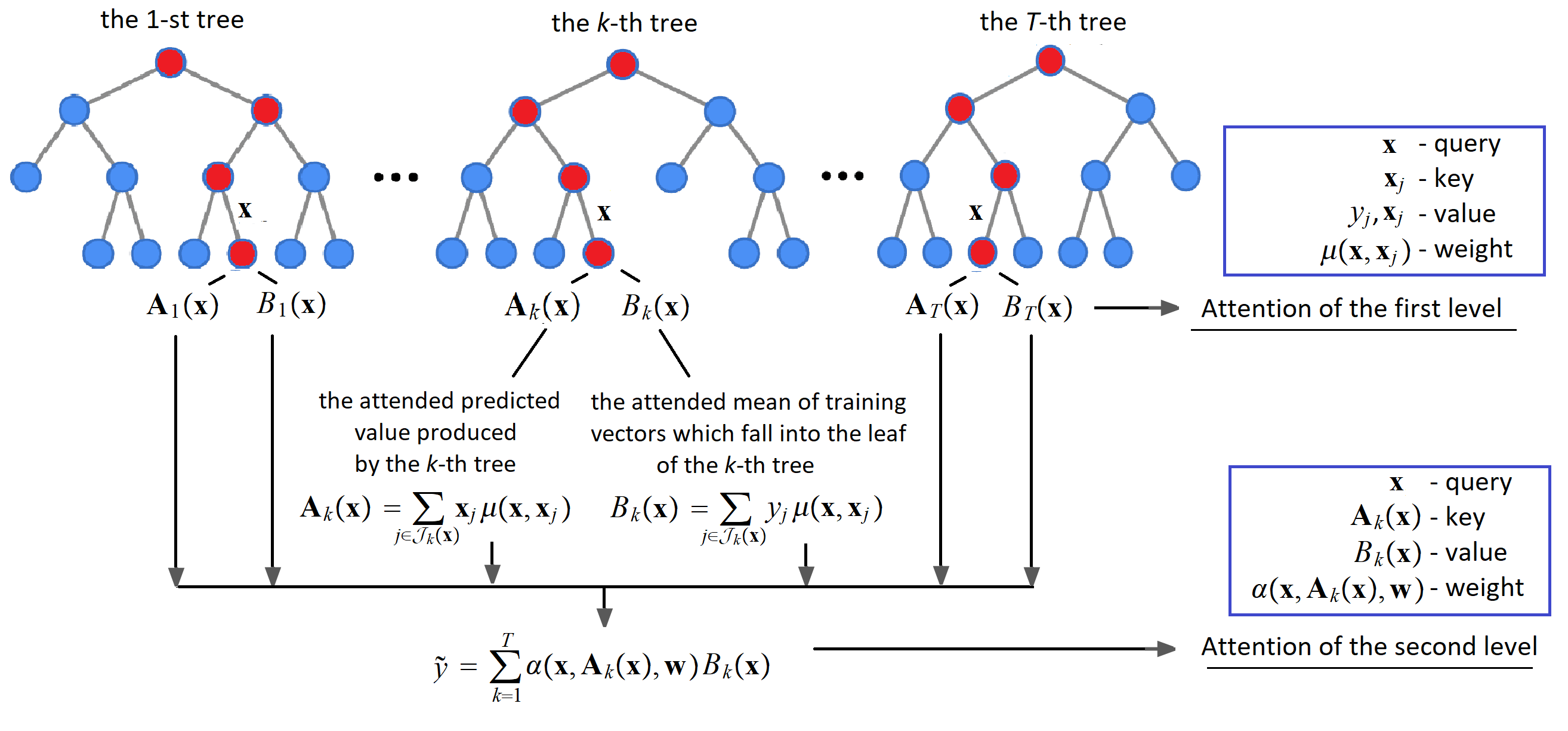
Figure 1: A scheme of the proposed two-level hierarchical attention model applied to the RF

Remark 1

It is important to point out that the additional sets of trainable parameters can be introduced into the definition of attention weights $\mu\left(\mathbf{x},\mathbf{x}_{j}\right)$. On the one hand, we get a more flexible attention mechanisms in this case due to the parametrization of training weights $\mu\left(\mathbf{x},\mathbf{x}_{j}\right)$. On the other hand, many trainable parameters lead to increasing complexity of the optimization problem (11) and to the possible overfitting of the whole RF.

5 Modifications of the two-level attention-based random forest

Different configurations of LARF produce a set of models which depend on trainable parameters of the two-level attention and its implementation. A classification of models and their notations are shown in Table 1. In order to explain the classification, two subsets of the attention parameters should be considered:

1. Parameters produced by contamination probability distributions of the Huber’s $\epsilon$-contamination model in the form of a vector $\mathbf{w}$ whose length coincides with the number of trees.

2. Parameters $\epsilon_{1},...,\epsilon_{M}$ of contamination in the mixture of $M$ the Huber’s contamination models, which define imprecision of the mixture model.

The following models can be constructed depending on trainable parameters and on using the “leaf” attention, i.e., the two-level attention mechanism:

• $\epsilon$-ARF: the attention-based forest with learning $\epsilon$ as a attention parameter, but without training vector $\mathbf{w}$, i.e., $w_{k}=1/T$, $k=1,...,T$, and without the “leaf” attention;

• $\mathbf{w}$-ARF: the attention-based forest with learning vector $\mathbf{w}$ as the attention parameters and without the “leaf” attention;

• $\epsilon$-LARF: the attention-based forest with learning $\epsilon$ as a attention parameter, but without training vector $\mathbf{w}$ and with the “leaf” attention, i.e., by using the two-level attention mechanism;

• $\mathbf{w}$-LARF: the attention-based forest with learning vector $\mathbf{w}$ as the attention parameters and with the “leaf” attention, i.e., by using the two-level attention mechanism;

• $\epsilon$-$\mathbf{w}$-ARF: the attention-based forest with learning vector $\mathbf{w}$ and the parameter $\epsilon$ as the attention parameters and without the “leaf” attention;

• $\epsilon$-$\mathbf{w}$-LARF: the attention-based forest with learning vector $\mathbf{w}$ and the parameter $\epsilon$ as the attention parameters and with the “leaf” attention;

• $\epsilon M$-ARF: the attention-based forest with learning parameters $\epsilon_{1},...,\epsilon_{M}$ as the attention parameters, with $w_{k}=1/T$, $k=1,...,T$, and without the “leaf” attention;

• $\epsilon M$-LARF: the attention-based forest with learning parameters $\epsilon_{1},...,\epsilon_{M}$ as the attention parameters, with $w_{k}=1/T$, $k=1,...,T$, and with the “leaf” attention;

• $\epsilon M$-$\mathbf{w}$-ARF: the attention-based forest with learning vector $\mathbf{w}$ and the parameters $\epsilon_{1},...,\epsilon_{M}$ as the attention parameters and without the “leaf” attention;

• $\epsilon M$-$\mathbf{w}$-LARF: the attention-based forest with learning vector $\mathbf{w}$ and the parameters $\epsilon_{1},...,\epsilon_{M}$ as the attention parameters and with the “leaf” attention.

Models $\epsilon$-ARF, $\epsilon$-LARF, $\epsilon$-$\mathbf{w}$-ARF, $\epsilon$-$\mathbf{w}$-LARF are not presented in Table 1 because they are special cases of models $\epsilon M$-ARF, $\epsilon M$-LARF, $\epsilon M$-$\mathbf{w}$-ARF, $\epsilon M$-$\mathbf{w}$-LARF, respectively, by $M=1$.

Table 1: Classification of the attention-based RF models proposed and studied in the paper

	Tuning $\epsilon$		Trainable $\epsilon_{1},...,\epsilon_{M}$
	fixed $\mathbf{w}$	trainable $\mathbf{w}$	fixed $\mathbf{w}$	trainable $\mathbf{w}$
Without the “leaf” attention	-	$\mathbf{w}$-ARF	$\epsilon M$-ARF	$\epsilon M$-$\mathbf{w}$-ARF
With the “leaf” attention	-	$\mathbf{w}$-LARF	$\epsilon M$-LARF	$\epsilon M$-$\mathbf{w}$-LARF

5.1 Huber’s contamination model and the basic two-level attention

In order to simplify optimization problem (12) and to effectively solve it, we propose to represent the attention weights $\alpha\left(\mathbf{x},\mathbf{A}_{k}(\mathbf{x)},\mathbf{w}\right)$ by using the Huber’s $\epsilon$-contamination model [14]. The idea to represent the attention weight by means of the $\epsilon$-contamination model has been proposed in [10]. We use this idea to incorporate the $\epsilon$-contamination model into optimization problem (12) and to construct first modifications of LARF.

Let us give a brief introduction into the Huber’s $\epsilon$-contamination model. The model considers a set of probability distributions of the form $F(\mathbf{x})=(1-\epsilon)\cdot P(\mathbf{x})+\epsilon\cdot R$. Here $P(\mathbf{x})=(p_{1}(\mathbf{x}),...,p_{T}(\mathbf{x}))$ is a discrete probability distribution contaminated by another probability distribution denoted $R=(r_{1},...,r_{T})$ which can be arbitrary in the unit simplex having dimension $T$. It is important to note that the distribution $P$ depends on the feature vector $\mathbf{x}$, i.e., it is different for every vector $\mathbf{x}$, whereas the distribution $R$ does not depend on $\mathbf{x}$. Contamination parameter $\epsilon\in[0,1]$ controls the impact of the contamination probability distribution $R$ on the distribution $P(\mathbf{x})$. Since the distribution $R$ can be arbitrary, then the set the distributions $F$ forms a subset of the unit simplex such that its size depends on parameter $\epsilon$. If $\epsilon=0$, then the subset of distributions $F$ is reduced to the single distribution $P(\mathbf{x})$. In case of $\epsilon=1$, the set of $F(\mathbf{x})$ is the whole unit simplex.

Following the common definition of the attention weights through the softmax operation with the parameter $\tau$, we propose to define each probability in $P(\mathbf{x})$ as

$$p_{k}(\mathbf{x})=\sigma\left(-\left\|\mathbf{x}-\mathbf{A}_{k}(\mathbf{x)}\right\|^{2}/\tau\right).$$

This implies that distribution $P(\mathbf{x})$ characterizes how the feature vector $\mathbf{x}$ is far from the vector $\mathbf{A}_{k}(\mathbf{x)}$ in all trees of the RF. Let us suppose that the probability distribution $R$ is the vector of trainable parameters $\mathbf{w}$. The idea is to train parameters $\mathbf{w}$ to achieve the best accuracy of the RF. After substituting the softmax operation into the attention weight $\alpha$, we get:

$$\alpha\left(\mathbf{x},\mathbf{A}_{k}(\mathbf{x)},\mathbf{w}\right)=(1-\epsilon)\cdot\text{$\sigma$}\left(-\left\|\mathbf{x}-\mathbf{A}_{k}(\mathbf{x)}\right\|^{2}/\tau\right)+\epsilon\cdot w_{k},\ k=1,...,T.$$ (13)

One can see from (13) that the attention weight is linearly depends on trainable parameters $\mathbf{w}=(w_{1},...,w_{T})$. It is important to note that the attention weight assigned to the $k$-th tree depends only on the $k$-th parameter $w_{k}$, but not on other elements of vector $\mathbf{w}$. Parameter $\epsilon$ is a tuning parameter determined by means of the standard validation procedure. It should be noted that elements of vector $\mathbf{w}$ are probabilities. Hence, there holds

$$\sum_{k=1}^{T}w_{k}=1.\ w_{k}\geq 0,\ k=1,...,T.$$ (14)

This implies that set $\mathcal{W}$ is the unit simplex of the dimension $T$.

Let us return to the attention weight $\mu\left(\mathbf{x},\mathbf{x}_{j}\right)$ of the first level. The attention is non-parametric at the first level, therefore, the attention weight can be defined in the standard way by using the Gaussian kernel or the softmax operation with parameter $\tau_{0}$, i.e., there holds

$$\mu\left(\mathbf{x},\mathbf{x}_{j}\right)=\sigma\left(-\left\|\mathbf{x}-\mathbf{x}_{j}\right\|^{2}/\tau_{0}\right).$$ (15)

Finally, we can rewrite the loss function (12) by taking into account the above definitions of the attention weights as follows:

$$\min_{\mathbf{w\in}\mathcal{W}}\sum_{s=1}^{n}L\left(\tilde{y}(\mathbf{x}_{s}),y_{s},\mathbf{w}\right)$$

$$=\min_{\mathbf{w\in}\mathcal{W}}\sum_{s=1}^{n}\left(y_{s}-\sum_{k=1}^{T}\left((1-\epsilon)C_{k}(\mathbf{x}_{s})-\epsilon D_{k}(\mathbf{x}_{s})w_{k}\right)\right)^{2},$$ (16)

where

$$C_{k}(\mathbf{x}_{s}) =\sum\nolimits_{l\in\mathcal{J}_{k}(\mathbf{x}_{s})}y_{l}\cdot\sigma\left(-\frac{\left\|\mathbf{x}_{s}-\mathbf{x}_{l}\right\|^{2}}{\tau_{0}}\right)$$

$$\times\text{$\sigma$}\left(-\frac{\left\|\mathbf{x}-\sum\nolimits_{i\in\mathcal{J}_{k}(\mathbf{x}_{s})}\mathbf{x}_{i}\cdot\sigma\left(-\left\|\mathbf{x}_{s}-\mathbf{x}_{i}\right\|^{2}/\tau_{0}\right)\right\|^{2}}{\tau}\right),$$ (17)

$$D_{k}(\mathbf{x}_{s})=\sum\nolimits_{j\in\mathcal{J}_{k}(\mathbf{x}_{s})}y_{j}\cdot\sigma\left(-\frac{\left\|\mathbf{x}_{s}-\mathbf{x}_{j}\right\|^{2}}{\tau_{0}}\right).$$ (18)

One can see from the above that $C_{k}(\mathbf{x}_{s})$ and $D_{k}(\mathbf{x}_{s})$ do not depend on parameters $\mathbf{w}$. Therefore, the objective function (16) jointly with the simple constraints $\mathbf{w}\in\mathcal{W}$ or (14) is the standard quadratic optimization problem which can be solved by means of many available efficient algorithms. The corresponding model is called $\mathbf{w}$-LARF. The notation means that trainable parameters are $\mathbf{w}$. The same model without “leaf” attention is denoted as $\mathbf{w}$-ARF. It coincides with the model $\epsilon$-ABRF proposed in [10].

It should be noted that the problem (16) is similar to the optimization problem stated in [9, 10]. However, it turns out that the addition of the “leaf” attention significantly improves the RF as it will be shown by many numerical experiments with real data.

5.2 Models with trainable contamination parameter $\epsilon$

One of the important contributions to the work, which makes the proposed model different from the model presented in [9, 10], is the idea to learn the contamination parameter $\epsilon$ jointly with parameters $\mathbf{w}$. However, this idea leads to a complex optimization problem such that gradient-based algorithms have to be used. In order to avoid using these algorithms and to get a simple optimization problem, we consider two ways. The first way is just to assign the same value $1/T$ to all parameters $w_{k}$. Then the optimization problem (16) can be rewritten as

$$\min_{0\leq\epsilon\leq 1}\sum_{s=1}^{n}\left(y_{s}-\sum_{k=1}^{T}\left((1-\epsilon)C_{k}(\mathbf{x}_{s})-\epsilon D_{k}(\mathbf{x}_{s})\frac{1}{T}\right)\right)^{2}.$$ (19)

We get a simple quadratic optimization problem with one variable $\epsilon$. Let us call the corresponding model as $\epsilon$-LARF. The notation means that the trainable parameter is $\epsilon$. The same model without “leaf” attention is denoted as $\epsilon$-ARF.

Another way is to introduce new variables $\gamma_{k}=\epsilon w_{k}$, $k=1,...,T$. Then the optimization problem (16) can be rewritten as

$$\min_{\gamma_{1},...,\gamma_{T},\epsilon}\sum_{s=1}^{n}\left(y_{s}-(1-\epsilon)\sum_{k=1}^{T}C_{k}(\mathbf{x}_{s})-\sum_{k=1}^{T}\gamma_{k}D_{k}(\mathbf{x}_{s})\right)^{2},$$ (20)

subject to

$$\sum_{k=1}^{T}\gamma_{k}=\epsilon,\ \gamma_{k}\geq 0,\ k=1,...,T,$$ (21)

$$0+\varsigma\leq\epsilon\leq 1.$$ (22)

We again get the quadratic optimization problem with new optimization variables $\gamma_{1},...,\gamma_{T},\epsilon$ and linear constraints. The parameter $\varsigma$ takes a small value to avoid the case $\epsilon=0$. The corresponding model is denoted $\epsilon$-$\mathbf{w}$-LARF. The notation means that trainable parameters are $\mathbf{w}$ and $\epsilon$. The same model without “leaf” attention is denoted as $\epsilon$-$\mathbf{w}$-ARF.

5.3 Mixture of contamination models

Another important contribution is an attempt to search for an optimal value of the temperature parameter $\tau$ in (13) or in (17). We propose an approximate approach which can significantly improve the model. Let us introduce a finite set $\{\tau_{1},...,\tau_{M}\}$ of $M$ values of parameter $\tau$. Here $M$ can be regarded as a tuning integer parameter which impact on the number of all training parameters. Large values of $M$ may lead to a large number of training parameters and the corresponding overfitting. Small values of $M$ may lead to an inexact approximation of $\tau$.

Before considering how the optimization problem can be rewritten taking into account the above, we again return to the attention weight $\alpha$ in (13) and represent it as follows:

$$\alpha\left(\mathbf{x},\mathbf{A}_{k}(\mathbf{x)},w_{k}\right)=\frac{1}{M}\sum_{j=1}^{M}\alpha_{j}\left(\mathbf{x},\mathbf{A}_{k}(\mathbf{x)},w_{k}\right),$$ (23)

where

$$\alpha_{j}\left(\mathbf{x},\mathbf{A}_{k}(\mathbf{x)},w_{k}\right)=(1-\epsilon_{j})\text{$\sigma$}\left(-\frac{\left\|\mathbf{x}-\mathbf{A}_{k}(\mathbf{x)}\right\|^{2}}{\tau_{j}}\right)+\epsilon_{j}w_{k}.$$ (24)

We have a mixture of $M$ contamination models with different contamination parameters $\epsilon_{j}$. It is obvious that the sum of new weights $\alpha$ over $k=1,...,T$ is $1$ because the sum of each $\alpha_{j}\left(\mathbf{x},\mathbf{A}_{k}(\mathbf{x)},w_{k}\right)$ over $k=1,...,T$ is also $1$. Each $\alpha_{j}\left(\mathbf{x},\mathbf{A}_{k}(\mathbf{x)},w_{k}\right)$ forms a small simplex such that its center is defined by $\tau_{j}$ and its size is defined by $\tau_{j}$. The corresponding sets of possible attention weights are depicted in Fig. 2 where the unit simplex by $T=3$ includes small simplices corresponding to three ($M=3$) contamination models $\alpha_{j}\left(\mathbf{x},\mathbf{A}_{k}(\mathbf{x)},w_{k}\right)$, $j=1,2,3$, with different centers and different contamination parameters $\epsilon_{1},\epsilon_{2},\epsilon_{3}$. The “mean” simplex of weights $\alpha\left(\mathbf{x},\mathbf{A}_{k}(\mathbf{x)},w_{k}\right)$ is depicted by using dashed sides. Parameters $\mathbf{w}$ are optimized such that the attention weights will be located in the “mean” simplex.

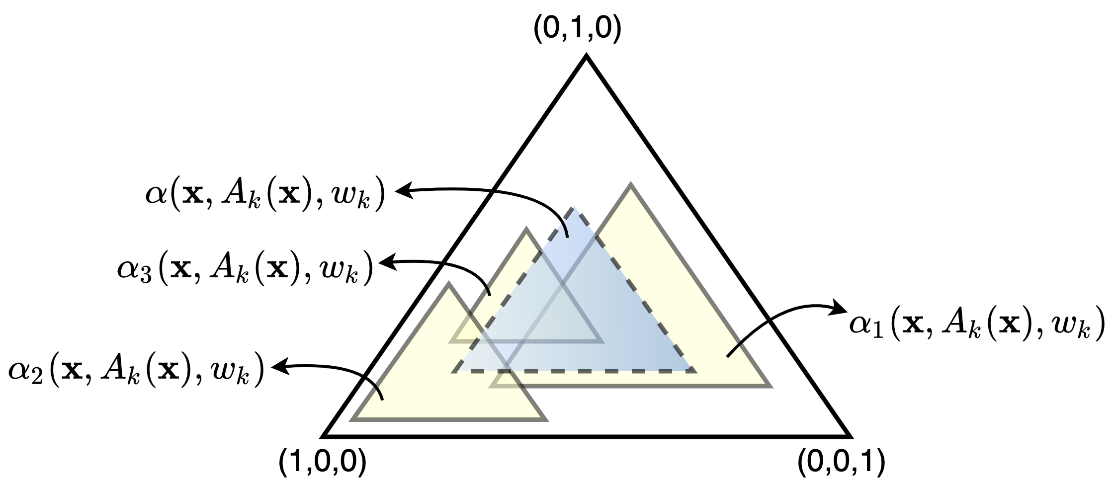
Figure 2: The unit simplex of possible attention weights which includes small simplices corresponding to three contamination models with different centers and different contamination parameters $\epsilon$ and the “mean” simplex (with dashed sides) which defines the set of final attention weights

Let us prove that the resulting “mean” model represents the $\epsilon$-contamination model with a contamination parameter $\epsilon$. Denote

$$P_{j}=\sigma\left(-\frac{\left\|\mathbf{x}-\mathbf{A}_{k}(\mathbf{x)}\right\|^{2}}{\tau_{j}}\right).$$ (25)

Here $P_{j}$ is a probability distribution, i.e., $P_{j}=(p_{j}^{(1)},...,p_{j}^{(T)})$. Then we can write

$$\alpha\left(\mathbf{x},\mathbf{A}_{k}(\mathbf{x)},w_{k}\right) =\frac{1}{M}\sum_{j=1}^{M}(1-\epsilon_{j})P_{j}+\frac{1}{M}\sum_{j=1}^{M}\epsilon_{j}w_{k}$$

$$=\frac{1}{M}\sum_{j=1}^{M}(1-\epsilon_{j})P_{j}+\epsilon w_{k},$$ (26)

where

$$\epsilon=\frac{1}{M}\sum_{j=1}^{M}\epsilon_{j}.$$ (27)

Suppose that there exists a probability distribution $Q=(q^{(1)},...,q^{(T)})$ such that there holds

$$\frac{1}{M}\sum_{j=1}^{M}(1-\epsilon_{j})P_{j}=(1-\epsilon)Q.$$ (28)

If we prove that the probability distribution $Q$ exists, then the resulting “mean” model is the $\epsilon$-contamination model. Let us find sums of the left and the right sides of (28) over $i=1,...,T$. Hence, we get

$$\frac{1}{M}\sum_{j=1}^{M}(1-\epsilon_{j})\sum_{i=1}^{T}p_{j}^{(i)}=(1-\epsilon)\sum_{i=1}^{T}q^{(i)}.$$ (29)

Substituting (27) into (29), we get

$$\sum_{i=1}^{T}q^{(i)}=1,$$

as was to be proved.

The introduced mixture of the contamination models can be regarded as a multi-head attention to some extent where every “head” is produced by using a certain parameter $\tau_{j}$.

Let us represent the softmax operation in (13) jointly with the factor $(1-\epsilon)$ as follows:

$$(1-\epsilon)\cdot\text{$\sigma$}\left(\frac{-\left\|\mathbf{x}-\mathbf{A}_{k}(\mathbf{x)}\right\|^{2}}{\tau}\right)=\frac{1}{M}\sum_{j=1}^{M}(1-\epsilon_{j})\cdot\text{$\sigma$}\left(\frac{-\left\|\mathbf{x}-\mathbf{A}_{k}(\mathbf{x)}\right\|^{2}}{\tau_{j}}\right).$$ (30)

It can be seen from (30) that new parameters $\epsilon_{1},...,\epsilon_{M}$ along with $\tau_{1},...,\tau_{M}$ are introduced in place of $\epsilon$ and $\tau$, respectively. Term $(1-\epsilon)\cdot$ $C_{k}(\mathbf{x}_{s})$ in (16) and (17) is replaced with the following terms:

$$\frac{1}{M}\sum_{j=1}^{M}(1-\epsilon_{j})C_{k}^{(j)}(\mathbf{x}_{s}),$$ (31)

where

$$C_{k}^{(j)}(\mathbf{x}_{s}) =\sum\nolimits_{l\in\mathcal{J}_{k}(\mathbf{x}_{s})}y_{l}\cdot\sigma\left(-\frac{\left\|\mathbf{x}_{s}-\mathbf{x}_{l}\right\|^{2}}{\tau_{0}}\right)$$

$$\times\text{$\sigma$}\left(-\frac{\left\|\mathbf{x}_{s}-\sum\nolimits_{i\in\mathcal{J}_{k}(\mathbf{x}_{s})}\mathbf{x}_{i}\mu\left(\mathbf{x}_{s},\mathbf{x}_{i}\right)\right\|^{2}}{\tau_{j}}\right).$$ (32)

Finally, we get the following optimization problem:

$$\min_{\gamma_{1},...,\gamma_{T},\epsilon}\sum_{s=1}^{n}\left(y_{s}-\frac{1}{M}\sum_{j=1}^{M}(1-\epsilon_{j})\sum_{k=1}^{T}C_{k}^{(j)}(\mathbf{x}_{s})\right.$$

$$\left.-\frac{1}{M}\sum_{j=1}^{M}\epsilon_{j}\sum_{k=1}^{T}w_{k}D_{k}(\mathbf{x}_{s})\right)^{2},$$ (33)

subject to

$$\sum_{k=1}^{T}w_{k}=1,~{}w_{k}\geq 0,~{}k=1,...,T.$$

Introduce new variables $\gamma_{k}^{(j)}=w_{k}\epsilon_{j}$, $k=1,...,T$, $j=1,...,M$. Hence we can write the optimization problem with new $M\cdot T+M$ variables as

$$\min_{\gamma_{1},...,\gamma_{T},\epsilon}\sum_{s=1}^{n}\left(y_{s}-\frac{1}{M}\sum_{j=1}^{M}(1-\epsilon_{j})\sum_{k=1}^{T}C_{k}^{(j)}(\mathbf{x}_{s})\right.$$

$$\left.-\frac{1}{M}\sum_{j=1}^{M}\sum_{k=1}^{T}\gamma_{k}^{(j)}D_{k}(\mathbf{x}_{s})\right)^{2},$$ (34)

subject to

$$\sum_{k=1}^{T}\gamma_{k}^{(j)}=\epsilon_{j},\ \gamma_{k}^{(j)}\geq 0,\ k=1,...,T,~{},j=1,...,M,$$ (35)

$$0+\varsigma\leq\epsilon_{j}\leq 1.$$ (36)

We again get the quadratic optimization problem with linear constraints. The corresponding model will be denoted as $\epsilon M$-$\mathbf{w}$-ARF or $\epsilon M$-$\mathbf{w}$-LARF depending on the applying the “leaf” attention. The notation means that trainable parameters are $\mathbf{w}$ and $\epsilon_{1},...,\epsilon_{M}$. We also will use the same model, but with condition $w_{k}=1/T$ for all $k=1,...,T$. The corresponding models are denoted as $\epsilon M$-ARF or $\epsilon M$-LARF.

6 Numerical experiments

Let is introduce notation for different models of the attention-based RFs.

1. RF (ERT): the original RF (the ERT) without applying the attention mechanisms;

2. ARF (LARF): the attention-based forest having the following modifications: $\epsilon M$-ARF, $\epsilon M$-LARF, $\epsilon M$-$\mathbf{w}$-ARF, $\epsilon M$-$\mathbf{w}$-LARF.

In all experiments, RFs as well as ERTs consist of $100$ trees. For selecting the best tuning parameters in numerical experiments, a 3-fold cross-validation on the training set consisting of $n_{\text{tr}}=4n/5$ examples with $100$ repetitions is performed. The search for the best parameter $\tau_{0}$ is carried out by considering all its values in a predefined grid. A cross-validation procedure is subsequently used to select their appropriate values. The testing set for computing the accuracy measures consists of $n_{\text{test}}=n/5$ examples. In order to get desirable estimates of vectors $\mathbf{A}_{k}(\mathbf{x})$ and $B_{k}(\mathbf{x})$, all trees in experiments are trained such that at least $10$ examples fall into every leaf of trees.

We do not consider models $\epsilon$-ARF, $\mathbf{w}$-ARF, $\epsilon$-LARF, $\mathbf{w}$-LARF because they can be regarded as special cases of the corresponding models $\epsilon$$M$-ARF, $\epsilon M$-$\mathbf{w}$-ARF, $\epsilon$$M$-LARF, $\epsilon M$-$\mathbf{w}$-LARF when $M=1$. The value of $M$ is taken $10$. Set $\{\tau_{1},...,\tau_{M}\}$ of the softmax operation parameters is defined as $\left\{10^{-\left\lfloor M/2\right\rfloor},10^{-\left\lfloor M/2\right\rfloor+1},...,10^{0},...,10^{\left\lfloor M/2\right\rfloor-1},10^{\left\lfloor M/2\right\rfloor}\right\}$. In particular, if $M=1$, then the set of $\tau$ consists of one element $\tau=1$. Parameter of the first-level attention in “leaf” $\tau_{0}$ is taken equal to $1$.

Numerical results are presented in tables where the best results are shown in bold. The coefficient of determination denoted $R^{2}$ and the mean absolute error (MAE) are used for the regression evaluation. The greater the value of the coefficient of determination and the smaller the MAE, the better results we get.

The proposed approach is studied by applying datasets which are taken from open sources. The dataset Diabetes is downloaded from the R Packages; datasets Friedman 1, 2 and 3 are taken at site: https://www.stat.berkeley.edu/~breiman/bagging.pdf; datasets Regression and Sparse are taken from package “Scikit-Learn”; datasets Wine Red, Boston Housing, Concrete, Yacht Hydrodynamics, Airfoil can be found in the UCI Machine Learning Repository [45]. These datasets with their numbers of features $m$ and numbers of examples $n$ are given in Table 2. A more detailed information can be found from the aforementioned data resources.

Table 2: A brief introduction about the regression data sets

Data set	Abbreviation	$m$	$n$
Diabetes	Diabetes	$10$	$442$
Friedman 1	Friedman 1	$10$	$100$
Friedman 2	Friedman 2	$4$	$100$
Friedman 3	Friedman 3	$4$	$100$
Scikit-Learn Regression	Regression	$100$	$100$
Scikit-Learn Sparse Uncorrelated	Sparse	$10$	$100$
UCI Wine red	Wine	$11$	$1599$
UCI Boston Housing	Boston	$13$	$506$
UCI Concrete	Concrete	$8$	$1030$
UCI Yacht Hydrodynamics	Yacht	$6$	$308$
UCI Airfoil	Airfoil	$5$	$1503$

Values of the measure $R^{2}$ for several models, including RF, $\epsilon M$-$\mathbf{w}$-ARF, $\epsilon M$-$\mathbf{w}$-LARF, $\epsilon M$-ARF and $\epsilon M$-LARF, are shown in Table 3. The results are obtained by training the RF. Optimal values of $\tau_{0}$ are also given in the table. It can be seen from Table 3 that $\epsilon M$-$\mathbf{w}$-LARF outperforms all models for most datasets. Moreover, one can see from Table 3 that the two-level attention models ($\epsilon M$-$\mathbf{w}$-LARF and $\epsilon M$-LARF) provide better results than models which do not use the “leaf” attention ($\epsilon M$-$\mathbf{w}$-ARF and $\epsilon M$-ARF). It should be also noted that all attention-based models outperform the original RF. The same relationship between the models takes place for another accuracy measure (MAE). It is clearly shown in Table 4.

Table 3: Values of $R^{2}$ for comparison of models based on the RF

Data set	$\tau_{0}$	RF	$\epsilon M$-$\mathbf{w}$-ARF	$\epsilon M$-$\mathbf{w}$-LARF	$\epsilon M$-ARF	$\epsilon M$-LARF
Diabetes	$0.01$	$0.416$	$0.419$	$\mathbf{0}$.$\mathbf{434}$	$0.425$	$0.426$
Friedman 1	$1$	$0.459$	$0.470$	$\mathbf{0}$.$\mathbf{524}$	$0.438$	$0.472$
Friedman 2	$1$	$0.841$	$0.887$	$\mathbf{0}$.$\mathbf{933}$	$0.886$	$0.916$
Friedman 3	$1$	$0.625$	$0.708$	$\mathbf{0}$.$\mathbf{749}$	$0.675$	$0.704$
Airfoil	$100$	$0.823$	$0.844$	$0.914$	$0.822$	$\mathbf{0}$.$\mathbf{917}$
Boston	$1$	$0.814$	$0.820$	$\mathbf{0}$.$\mathbf{870}$	$0.819$	$0.856$
Concrete	$10$	$0.845$	$0.857$	$\mathbf{0}$.$\mathbf{896}$	$0.844$	$\mathbf{0}$.$\mathbf{896}$
Wine	$1$	$0.433$	$0.421$	$\mathbf{0}$.$\mathbf{481}$	$0.421$	$0.477$
Yacht	$0.1$	$0.981$	$0.989$	$\mathbf{0}$.$\mathbf{993}$	$0.981$	$0.982$
Regression	$0.1$	$0.380$	$0.434$	$\mathbf{0}$.$\mathbf{455}$	$0.361$	$0.409$
Sparse	$1$	$0.470$	$0.489$	$\mathbf{0}$.$\mathbf{641}$	$0.535$	$0.630$

Table 4: Values of MAE for comparison of models based on the RF

Data set	RF	$\epsilon M$-$\mathbf{w}$-ARF	$\epsilon M$-$\mathbf{w}$-LARF	$\epsilon M$-ARF	$\epsilon M$-LARF
Diabetes	$44.92$	$44.95$	$\mathbf{44}$.$\mathbf{61}$	$44.79$	$44.81$
Friedman 1	$2.540$	$2.545$	$\mathbf{2}$.$\mathbf{411}$	$2.595$	$2.473$
Friedman 2	$111.7$	$95.29$	$\mathbf{72}$.$\mathbf{71}$	$92.44$	$74.24$
Friedman 3	$0.154$	$0.130$	$0.135$	$0.144$	$\mathbf{0}$.$\mathbf{129}$
Airfoil	$2.203$	$2.065$	$1.451$	$2.217$	$\mathbf{1}$.$\mathbf{416}$
Boston	$2.539$	$2.538$	$\mathbf{2}$.$\mathbf{148}$	$2.489$	$2.217$
Concrete	$4.834$	$4.676$	$\mathbf{3}$.$\mathbf{496}$	$4.883$	$3.615$
Wine	$0.451$	$0.459$	$\mathbf{0}$.$\mathbf{411}$	$0.461$	$0.417$
Yacht	$1.004$	$0.787$	$\mathbf{0}$.$\mathbf{611}$	$1.004$	$0.971$
Regression	$109.1$	$103.6$	$\mathbf{101}$.$\mathbf{3}$	$111.2$	$105.8$
Sparse	$1.908$	$1.871$	$\mathbf{1}$.$\mathbf{528}$	$1.772$	$1.543$

Another important question is how the attention-based models perform when the ERT is used. The corresponding values of $R^{2}$ and MAE are shown in Tables 5 and 6, respectively. Table 5 also contains optimal values $\tau_{0}$. In contrast to the case of using the RF, it can be seen from the tables that $\epsilon M$-LARF outperforms $\epsilon M$-$\mathbf{w}$-LARF for several models. It can be explained by reducing the accuracy due to a larger number of training parameters (parameters $\mathbf{w}$) and overfitting for small datasets. It is also interesting to note that models based on ERTs provide better results than models based on RFs. However, this improvement is not significant. This is clearly seen from Table 7 where the best results are collected for models based on ERTs and RFs. One can see from Table 7 that results are identical for several datasets, namely, for datasets Friedman 1, 2, 3, Concrete, Yacht. If to apply the $t$-test to compare values of $R^{2}$ obtained for two models, then, according to [46], the $t$-statistics is distributed in accordance with the Student distribution with $11-1$ degrees of freedom ($11$ datasets). The obtained p-value is $p=0.071$. We can conclude that the outperformance of the ERT is not statistically significant because $p>0.05$.

Table 5: Values of $R^{2}$ for comparison of models based on the ERT

Data set	$\tau_{0}$	ERT	$\epsilon M$-$\mathbf{w}$-ARF	$\epsilon M$-$\mathbf{w}$-LARF	$\epsilon M$-ARF	$\epsilon M$-LARF
Diabetes	$0.01$	$0.438$	$0.441$	$0.434$	$\mathbf{0}$.$\mathbf{471}$	$0.444$
Friedman 1	$1$	$0.471$	$0.471$	$\mathbf{0}$.$\mathbf{524}$	$0.441$	$0.495$
Friedman 2	$10$	$0.813$	$0.840$	$\mathbf{0}$.$\mathbf{933}$	$0.840$	$0.919$
Friedman 3	$1$	$0.570$	$0.569$	$\mathbf{0}$.$\mathbf{749}$	$0.569$	$0.637$
Airfoil	$100$	$0.802$	$0.804$	$\mathbf{0}$.$\mathbf{914}$	$0.804$	$0.909$
Boston	$10$	$0.831$	$0.834$	$0.870$	$0.834$	$\mathbf{0}$.$\mathbf{882}$
Concrete	$10$	$0.839$	$0.838$	$\mathbf{0}$.$\mathbf{896}$	$0.838$	$0.895$
Wine	$1$	$0.418$	$0.418$	$0.481$	$0.418$	$\mathbf{0}$.$\mathbf{486}$
Yacht	$1$	$0.988$	$0.988$	$\mathbf{0}$.$\mathbf{993}$	$0.988$	$\mathbf{0}$.$\mathbf{993}$
Regression	$0.1$	$0.402$	$0.429$	$0.455$	$0.429$	$\mathbf{0}$.$\mathbf{464}$
Sparse	$1$	$0.452$	$0.522$	$0.641$	$0.522$	$\mathbf{0}$.$\mathbf{663}$

Table 6: Values of MAE for comparison of models based on the ERT

Data set	ERT	$\mathbf{w}$-ARF	$\mathbf{w}$-LARF	$\epsilon M$-ARF	$\epsilon M$-LARF
Diabetes	$44.549$	$44.271$	$44.614$	$44.271$	$\mathbf{44}$.$\mathbf{21}$
Friedman 1	$2.502$	$2.502$	$2.411$	$2.502$	$\mathbf{2}$.$\mathbf{388}$
Friedman 2	$123.0$	$113.7$	$72.71$	$113.7$	$\mathbf{70}$.$\mathbf{48}$
Friedman 3	$0.179$	$0.179$	$\mathbf{0}$.$\mathbf{135}$	$0.179$	$0.148$
Airfoil	$2.370$	$2.360$	$\mathbf{1}$.$\mathbf{451}$	$2.360$	$1.471$
Boston	$2.481$	$2.451$	$2.148$	$2.451$	$\mathbf{2}$.$\mathbf{023}$
Concrete	$5.119$	$5.124$	$\mathbf{3}$.$\mathbf{496}$	$5.124$	$3.659$
Wine	$0.464$	$0.464$	$\mathbf{0}$.$\mathbf{411}$	$0.464$	$0.412$
Yacht	$0.824$	$0.822$	$\mathbf{0}$.$\mathbf{611}$	$0.822$	$0.612$
Regression	$106.3$	$103.1$	$101.3$	$103.1$	$\mathbf{100}$.$\mathbf{0}$
Sparse	$1.994$	$1.820$	$1.528$	$1.820$	$\mathbf{1}$.$\mathbf{519}$

Table 7: Comparison of the best results provided by models based on RFs and ERTs

Data set	RF	ERT
Diabetes	$0.434$	$\mathbf{0}$.$\mathbf{471}$
Friedman 1	$\mathbf{0}$.$\mathbf{524}$	$\mathbf{0}$.$\mathbf{524}$
Friedman 2	$\mathbf{0}$.$\mathbf{933}$	$\mathbf{0}$.$\mathbf{933}$
Friedman 3	$\mathbf{0}$.$\mathbf{749}$	$\mathbf{0}$.$\mathbf{749}$
Airfoil	$\mathbf{0}$.$\mathbf{917}$	$0.914$
Boston	$0.870$	$\mathbf{0}$.$\mathbf{882}$
Concrete	$\mathbf{0}$.$\mathbf{896}$	$\mathbf{0}$.$\mathbf{896}$
Wine	$0.481$	$\mathbf{0}$.$\mathbf{486}$
Yacht	$\mathbf{0}$.$\mathbf{993}$	$\mathbf{0}$.$\mathbf{993}$
Regression	$0.455$	$\mathbf{0}$.$\mathbf{464}$
Sparse	$0.641$	$\mathbf{0}$.$\mathbf{663}$

It should be pointed out that the proposed models can be regarded as extensions of the attention-based RF ($\epsilon$-ABRF) presented in [10]. Therefore, it is also interesting to compare the two-level attention models with $\epsilon$-ABRF. Table 8 shows values of $R^{2}$ obtained by using $\epsilon$-ABRF and the best values of proposed models when the RF and the ERT are used.

If to formally compare results presented in Table 8 by applying the $t$-tests in accordance with [46], then tests for the proposed models and $\epsilon$-ABRF based on the RF and the ERT provide p-values equal to $p=0.00067$ and $p=0.00029$, respectively. The tests demonstrate the clear outperformance of the proposed models in comparison with $\epsilon$-ABRF.

Table 8: Comparison of $\epsilon$-ABRF and the proposed models by using the measure $R^{2}$ when RFs and ERTs are the basis

	RF		ERT
Data set	$\epsilon$-ABRF	LARF	$\epsilon$-ABRF	LARF
Diabetes	$0.424$	$\mathbf{0.434}$	$0.441$	$\mathbf{0.471}$
Friedman 1	$0.470$	$\mathbf{0.524}$	$0.513$	$\mathbf{0.524}$
Friedman 2	$0.877$	$\mathbf{0.933}$	$0.930$	$\mathbf{0.933}$
Friedman 3	$0.686$	$\mathbf{0.749}$	$0.739$	$\mathbf{0.749}$
Airfoil	$0.843$	$\mathbf{0.917}$	$0.837$	$\mathbf{0.914}$
Boston	$0.823$	$\mathbf{0.870}$	$0.838$	$\mathbf{0.882}$
Concrete	$0.857$	$\mathbf{0.896}$	$0.863$	$\mathbf{0.896}$
Wine	$0.423$	$\mathbf{0.481}$	$0.416$	$\mathbf{0.486}$
Yacht	$0.989$	$\mathbf{0.993}$	$0.988$	$\mathbf{0.993}$
Regression	$0.450$	$\mathbf{0.455}$	$0.447$	$\mathbf{0.464}$
Sparse	$0.529$	$\mathbf{0.641}$	$0.536$	$\mathbf{0.663}$

7 Concluding remarks

New attention-based RF models proposed in the paper have supplemented the class attention models incorporated into machine learning models different from neural networks [9, 10]. Moreover, the proposed models do not use gradient-based algorithms to learn attention parameters, and their training is based on solving the quadratic optimization problem with linear constraints. This peculiarity significantly simplifies the training process.

It is interesting to point out that computing the attention weights in leaves of trees is a very simple task from the computational point of view. At the same time, this simple modification leads to the crucial improvement of the RF models. Numerical results with real data have demonstrated this improvement. This fact motivates us to continue developing attention-based modifications of machine learning models in different directions. First of all, the same approach can be applied to the gradient boosting machine [8]. The first successful attempt to use the attention mechanism in the gradient boosting machine with decision trees as base learners has been carried out in [9]. This attempt has been shown that the boosting model can be improved by adding the attention component. An idea of the “leaf” attention and the optimization over parameters of kernels can be directly transferred to the gradient boosting machine. This is a direction for further research.

One of the important results presented in the paper is the usage of a specific mixture of contamination models which can be regarded as a variant of the well-known multi-head attention [16], where each “head” is defined by the kernel parameter. However, values of the parameter are selected in accordance with a predefined set. Therefore, the next direction for research is to consider randomized procedures for selecting values of the parameter.

The proposed models consider only a single leaf of a tree for every example and implement the “leaf” attention in this leaf. However, they do not take into account neighbor leaves which also may provide useful information for improving the models. The corresponding modification can be also regarded as another direction for research.

It has been shown in [10] that attention-based RFs allow us to interpret predictions by using the attention weights. The introduced two-level attention mechanisms may also improve interpretability of RFs by taking into account additional factors. The corresponding procedures of the interpretation is also a direction for further research.

Finally, we have developed the proposed modifications by using the Huber’s $\epsilon$-contamination model and the mixture of the models. Another problem of interest is to consider different available statistical models [47] and their mixtures. A proper choice of the mixture components may significantly improve the whole attention-based RF. This is also a direction for further research.

References

- [1] S. Chaudhari, V. Mithal, G. Polatkan, and R. Ramanath. An attentive survey of attention models. arXiv:1904.02874, Apr 2019.
- [2] A.S. Correia and E.L. Colombini. Attention, please! A survey of neural attention models in deep learning. arXiv:2103.16775, Mar 2021.
- [3] A.S. Correia and E.L. Colombini. Neural attention models in deep learning: Survey and taxonomy. arXiv:2112.05909, Dec 2021.
- [4] T. Lin, Y. Wang, X. Liu, and X. Qiu. A survey of transformers. arXiv:2106.04554, Jul 2021.
- [5] Z. Niu, G. Zhong, and H. Yu. A review on the attention mechanism of deep learning. Neurocomputing, 452:48–62, 2021.
- [6] L. Breiman. Random forests. Machine learning, 45(1):5–32, 2001.
- [7] J.H. Friedman. Greedy function approximation: A gradient boosting machine. Annals of Statistics, 29:1189–1232, 2001.
- [8] J.H. Friedman. Stochastic gradient boosting. Computational statistics & data analysis, 38(4):367–378, 2002.
- [9] A.V. Konstantinov, L.V. Utkin, and S.R. Kirpichenko. AGBoost: Attention-based modification of gradient boosting machine. In 31st Conference of Open Innovations Association (FRUCT), pages 96–101. IEEE, 2022.
- [10] L.V. Utkin and A.V. Konstantinov. Attention-based random forest and contamination model. Neural Networks, 2022. In press.
- [11] A. Zhang, Z.C. Lipton, M. Li, and A.J. Smola. Dive into deep learning. arXiv:2106.11342, Jun 2021.
- [12] E.A. Nadaraya. On estimating regression. Theory of Probability & Its Applications, 9(1):141–142, 1964.
- [13] G.S. Watson. Smooth regression analysis. Sankhya: The Indian Journal of Statistics, Series A, pages 359–372, 1964.
- [14] P.J. Huber. Robust Statistics. Wiley, New York, 1981.
- [15] L.V. Utkin and A.V. Konstantinov. Attention and self-attention in random forests. arXiv:2207.04293, Jul 2022.
- [16] A. Vaswani, N. Shazeer, N. Parmar, J. Uszkoreit, L. Jones, A.N. Gomez, L. Kaiser, and I. Polosukhin. Attention is all you need. In Advances in Neural Information Processing Systems, pages 5998–6008, 2017.
- [17] P. Geurts, D. Ernst, and L. Wehenkel. Extremely randomized trees. Machine learning, 63:3–42, 2006.
- [18] F. Liu, X. Huang, Y. Chen, and J.A. Suykens. Random features for kernel approximation: A survey on algorithms, theory, and beyond. arXiv:2004.11154v5, Jul 2021.
- [19] K. Choromanski, V. Likhosherstov, D. Dohan, X. Song, A. Gane, T. Sarlos, P. Hawkins, J. Davis, A. Mohiuddin, L. Kaiser, D. Belanger, L. Colwell, and A. Weller. Rethinking attention with performers. In 2021 International Conference on Learning Representations, 2021.
- [20] K. Choromanski, H. Chen, H. Lin, Y. Ma, A. Sehanobish, D. Jain, M.S. Ryoo, J. Varley, A. Zeng, V. Likhosherstov, D. Kalachnikov, V. Sindhwani, and A. Weller. Hybrid random features. arXiv:2110.04367v2, Oct 2021.
- [21] X. Ma, X. Kong, S. Wang, C. Zhou, J. May, H. Ma, and L. Zettlemoyer. Luna: Linear unified nested attention. arXiv:2106.01540, Nov 2021.
- [22] I. Schlag, K. Irie, and J. Schmidhuber. Linear transformers are secretly fast weight programmers. In International Conference on Machine Learning 2021, pages 9355–9366. PMLR, 2021.
- [23] H. Peng, N. Pappas, D. Yogatama, R. Schwartz, N. Smith, and L. Kong. Random feature attention. In International Conference on Learning Representations (ICLR 2021), pages 1–19, 2021.
- [24] G. Brauwers and F. Frasincar. A general survey on attention mechanisms in deep learning. arXiv:2203.14263, Mar 2022.
- [25] T. Goncalves, I. Rio-Torto, L.F. Teixeira, and J.S. Cardoso. A survey on attention mechanisms for medical applications: are we moving towards better algorithms? arXiv:2204.12406, Apr 2022.
- [26] A. Santana and E. Colombini. Neural attention models in deep learning: Survey and taxonomy. arXiv:2112.05909, Dec 2021.
- [27] D. Soydaner. Attention mechanism in neural networks: Where it comes and where it goes. arXiv:2204.13154, Apr 2022.
- [28] Y. Xu, H. Wei, M. Lin, Y. Deng, K. Sheng, M. Zhang, F. Tang, W. Dong, F. Huang, and C. Xu. Transformers in computational visual media: A survey. Computational Visual Media, 8(1):33–62, 2022.
- [29] H. Kim, H. Kim, H. Moon, and H. Ahn. A weight-adjusted voting algorithm for ensemble of classifiers. Journal of the Korean Statistical Society, 40(4):437–449, 2011.
- [30] C.A. Ronao and S.-B. Cho. Random forests with weighted voting for anomalous query access detection in relational databases. In Artificial Intelligence and Soft Computing. ICAISC 2015, volume 9120 of Lecture Notes in Computer Science, pages 36–48, Cham, 2015. Springer.
- [31] L.V. Utkin, A.V. Konstantinov, V.S. Chukanov, and A.A. Meldo. A new adaptive weighted deep forest and its modifications. International Journal of Information Technology & Decision Making, 19(4):963–986, 2020.
- [32] L.V. Utkin, A.V. Konstantinov, V.S. Chuknov, M.V. Kots, M.A. Ryabinin, and A.A. Meldo. A weighted random survival forest. arXiv:1901.00213, Jan 2019.
- [33] S.J. Winham, R.R. Freimuth, and J.M. Biernacka. A weighted random forests approach to improve predictive performance. Statistical Analysis and Data Mining, 6(6):496–505, 2013.
- [34] S. Xuan, G. Liu, and Z. Li. Refined weighted random forest and its application to credit card fraud detection. In Computational Data and Social Networks, pages 343–355, Cham, 2018. Springer International Publishing.
- [35] X. Zhang and M. Wang. Weighted random forest algorithm based on bayesian algorithm. In Journal of Physics: Conference Series, volume 1924, pages 1–6. IOP Publishing, 2021.
- [36] J. Abellan and S. Moral. Building classification trees using th building classification trees using the total uncertainty criterion. International Journal of Intelligent Systems, 18(12):1215–1225, 2003.
- [37] J. Abellan, C.J. Mantas, and J.G. Castellano. A random forest approach using imprecise probabilities. Knowledge-Based Systems, 134:72–84, 2017.
- [38] J. Abellan, C.J. Mantas, J.G. Castellano, and S. Moral-Garcia. Increasing diversity in random forest learning algorithm via imprecise probabilities. Expert Systems With Applications, 97:228–243, 2018.
- [39] C.J. Mantas and J. Abellan. Analysis and extension of decision trees based on imprecise probabilities: Application on noisy data. Expert Systems with Applications, 41(5):2514–2525, 2014.
- [40] S. Moral-Garcia, C.J. Mantas, J.G. Castellano, M.D. Benitez, and J. Abellan. Bagging of credal decision trees for imprecise classification. Expert Systems with Applications, 141(Article 112944):1–9, 2020.
- [41] L.V. Utkin and A. Wiencierz. An imprecise boosting-like approach to regression. In Fabio Cozman, Therry Denoeux, Sébastien Destercke, and Teddy Seidfenfeld, editors, ISIPTA ’13, Proceedings of the Eighth International Symposium on Imprecise Probability: Theories and Applications, pages 345–354, Compiegne, France, 2013. SIPTA.
- [42] L.V. Utkin, M.S. Kovalev, and F. Coolen. Imprecise weighted extensions of random forests for classification and regression. Applied Soft Computing, 92(Article 106324):1–14, 2020.
- [43] D. Bahdanau, K. Cho, and Y. Bengio. Neural machine translation by jointly learning to align and translate. arXiv:1409.0473, Sep 2014.
- [44] T. Luong, H. Pham, and C.D. Manning. Effective approaches to attention-based neural machine translation. In Proceedings of the 2015 Conference on Empirical Methods in Natural Language Processing, pages 1412–1421. The Association for Computational Linguistics, 2015.
- [45] D. Dua and C. Graff. UCI machine learning repository, 2017.
- [46] J. Demsar. Statistical comparisons of classifiers over multiple data sets. Journal of Machine Learning Research, 7:1–30, 2006.
- [47] P. Walley. Statistical Reasoning with Imprecise Probabilities. Chapman and Hall, London, 1991.