Contrastive Trajectory Similarity Learning with Dual-Feature Attention

Abstract

Trajectory similarity measures act as query predicates in trajectory databases, making them the key player in determining the query results. They also have a heavy impact on the query efficiency. An ideal measure should have the capability to accurately evaluate the similarity between any two trajectories in a very short amount of time. Towards this aim, we propose a contrastive learning-based trajectory modeling method named TrajCL. We present four trajectory augmentation methods and a novel dual-feature self-attention-based trajectory backbone encoder. The resultant model can jointly learn both the spatial and the structural patterns of trajectories. Our model does not involve any recurrent structures and thus has a high efficiency. Besides, our pre-trained backbone encoder can be fine-tuned towards other computationally expensive measures with minimal supervision data. Experimental results show that TrajCL is consistently and significantly more accurate than the state-of-the-art trajectory similarity measures. After fine-tuning, i.e., to serve as an estimator for heuristic measures, TrajCL can even outperform the state-of-the-art supervised method by up to 56% in the accuracy for processing trajectory similarity queries.

I Introduction

A trajectory is commonly represented as a sequence of location points to describe the movement of an object, such as a person or a vehicle. Measuring the similarity between trajectories is a fundamental step in trajectory queries [1, 2, 3, torchdison, 4, 5, 6], since it is used as a query predicate which determines query results and efficiency. Unlike numeric data and character data, there are not many universally applicable comparison criteria for trajectory data, and thus measuring similarity between trajectories is an important area of research.

A series of trajectory similarity measures [7, 8, 9, 10, 11, 12, 13] have been proposed, which can be classified into two categories: heuristic measures and learned measures. Heuristic trajectory similarity measures [7, 8, 9, 10] mainly aim to find a point-oriented matching between two trajectories based on hand-crafted rules. For example, Hausdorff [9] leverages the Euclidean distances between points on two trajectories to measure trajectory similarity. Learned trajectory similarity measures [11, 12, 13, 14], on the other hand, utilize deep learning models to predict similarity values by computing the distance between trajectory-oriented embeddings (i.e., numeric vector representations of trajectories). For example, t2vec [11] and E2DTC [14] adapt recurrent neural networks (RNN) to encode trajectories into embeddings, TrjSR [12] uses convolutional neural networks (CNN) to embed trajectories.

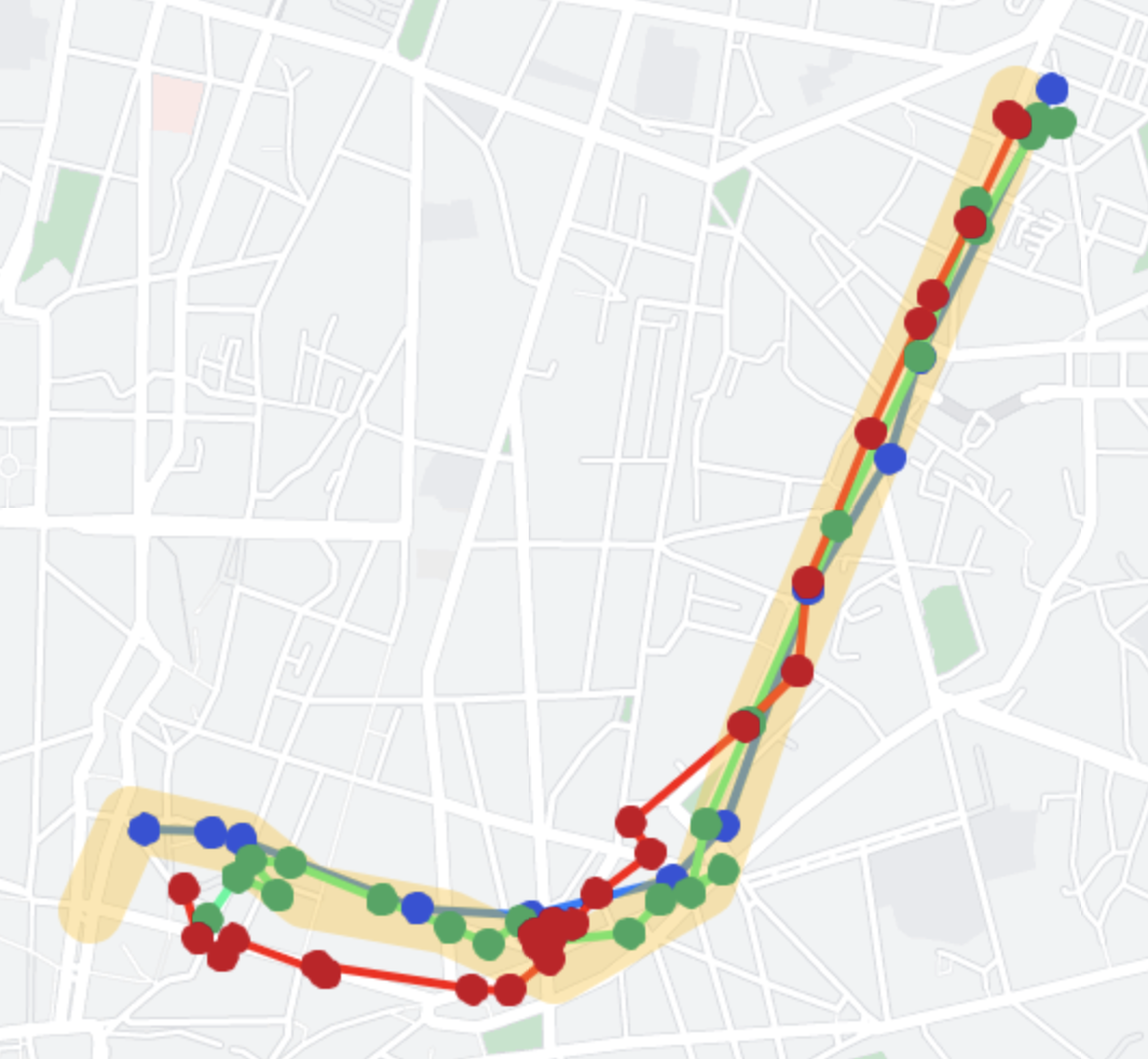
(a) Hausdorff (heuristic) 

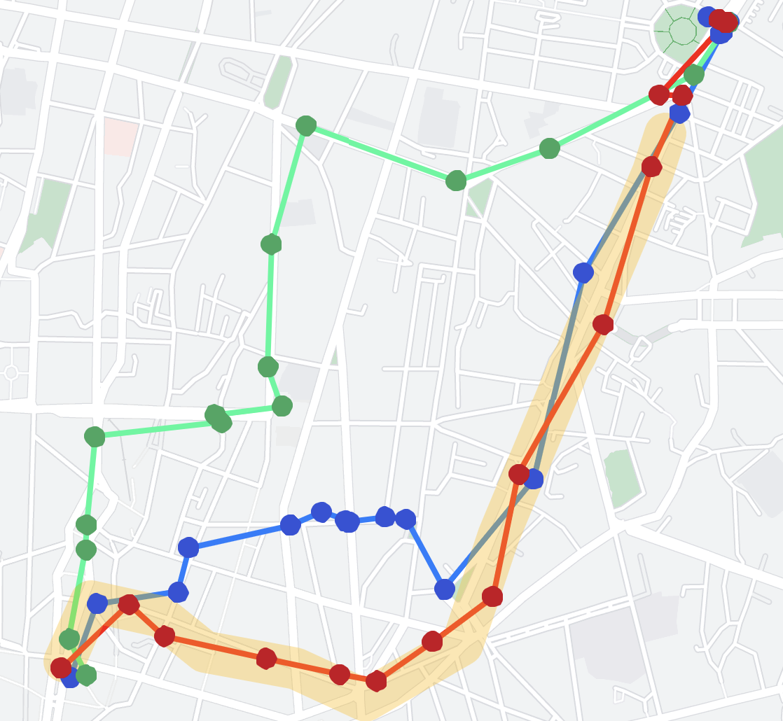
(b) t2vec (learned) 

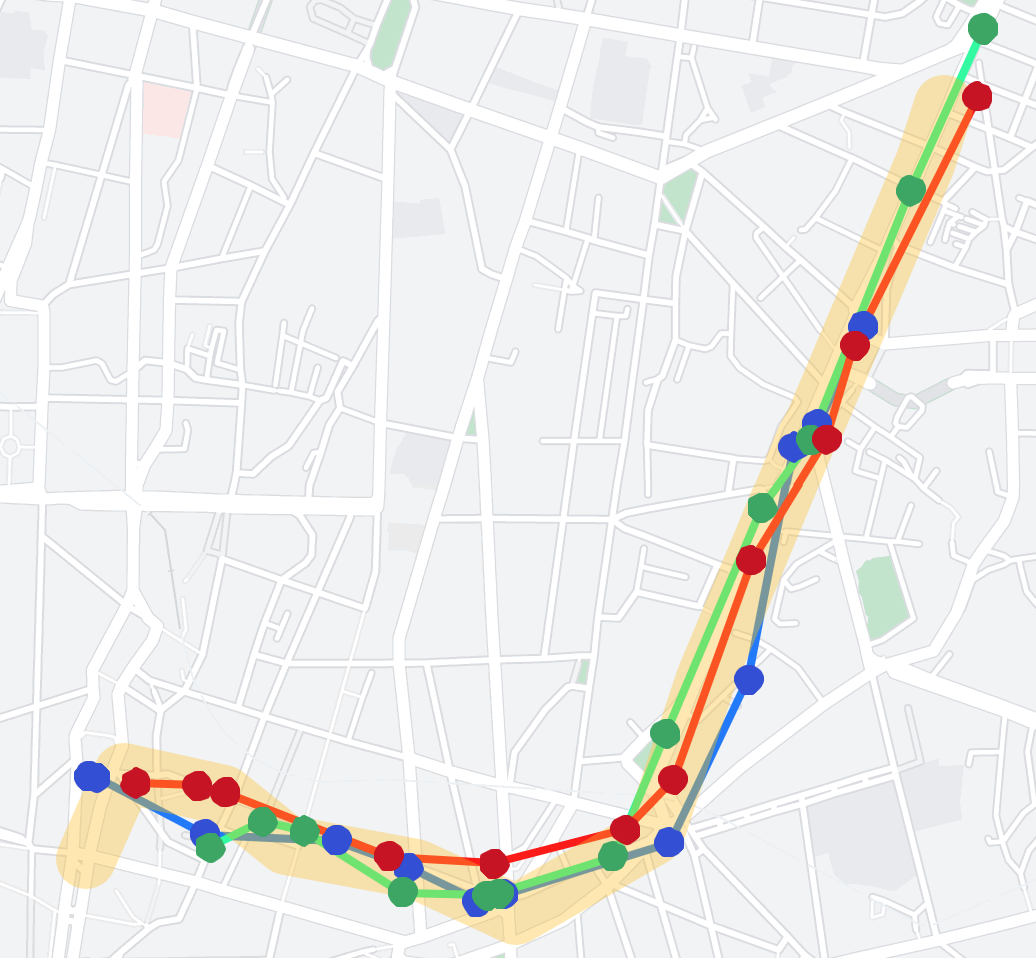
(c) TrajCL (ours) 

Figure 1: Querying the $3$NN trajectories (The query trajectory is in yellow with extra thick lines for easy viewing. The $3$NN results are colored in red, green and blue, respectively.)

TABLE I: Trajectory similarity computation time

3	Hausdorff	t2vec	TrajCL
Time ($\mu$s)	6.63	0.34	0.14
3

Measures in the both categories above face the following challenges. (1) Ineffectiveness: Trajectories with different sampling rates or containing noise can degrade the effectiveness of the existing measures. This is because the heuristic measures using hand-crafted rules are prone to errors by low-quality trajectories. The learned measures also suffer from this problem, since they mostly adopt deep learning models which are not originally designed for trajectory data and may fail to capture long spatial correlations between trajectory points and between similar trajectories. For example, Fig. 1 shows the 3-nearest neighbor query results on the Porto taxi trajectory dataset [15]. The query results obtained using t2vec (Fig. 1b) are far from the query trajectory. Those obtained by Hausdorff are closer to the query trajectory (Fig. 1a), but not as close as those obtained by our TrajCL method (Fig. 1c), while Hausdorff suffers in efficiency (discussed next). (2) Inefficiency: Existing heuristic measures compute the distance between each pair of points on two trajectories. They take at least a quadratic time w.r.t. the number of trajectory points, which is unacceptable in online systems, especially when trajectories become longer. Although the learned measures get rid of pairwise point comparisons, they are still limited in efficiency. As Table I shows, Hausdorff takes 6.63 microseconds to compute the similarity of two Porto taxi trajectories. t2vec reduces the time by more than an order of magnitude to 0.34 microseconds. However, its recurrent structure has not fully exploited the parallel power of GPUs. Our TrajCL avoids this recurrent structure and further brings the computation time down to 0.14 microseconds.

To address these issues, we propose TrajCL, a contrastive learning-based trajectory similarity measure with a dual-feature self-attention-based trajectory backbone encoder (DualSTB). TrajCL first leverages our proposed trajectory augmentation methods to generate diverse trajectory variants (i.e., so called views) with different characteristics for each training sample. Then, the proposed DualSTB encoder embeds the augmented trajectories into trajectory embeddings, which can capture the spatial distance correlation between the trajectories. After that, we compute the similarity of two trajectories simply as the $L_{1}$ distance between their embeddings.

Due to the lack of ground-truth for trajectory similarity, we train our proposed DualSTB encoder by adopting self-supervised contrastive learning [16, 17] that aims to maximize the agreement between the representations of positive (i.e., similar) data pairs and minimize that of the negative (i.e., dissimilar) data pairs, where the positive and negative data pairs are generated from input data via augmentation methods.

The idea of using contrastive learning for representation learning is not new. By introducing it into trajectory embedding learning, our first technical contribution is four trajectory augmentation methods that enable obtaining the positive and negative data pairs for contrastive learning over trajectories. These methods include point shifting, point masking, trajectory truncating, and trajectory simplification. The augmented trajectories can be regarded as a set of low-quality variants of the input trajectories with uncertainty. Such diverse trajectories guide our model to learn the key patterns to differentiate between similar and not-so-similar trajectory pairs.

Our second technical contribution is a dual-feature self-attention-based trajectory backbone encoder (i.e., DualSTB) that encodes both structural and spatial trajectory features of a trajectory into its learned embedding. The two types of features together provide coarse-grained and fine-grained location information of trajectories. To obtain a comprehensive embedding based on the two types of features, we devise a dual-feature multi-head self-attention module that first learns the correlations between trajectory points based on each type of features. Then, the module adaptively combines the two types of correlations, and finally it forms the output embeddings. Such a module can capture the long-term dependency between trajectory points, while its non-recurrent structure enables model inference with high efficiency.

After TrajCL is trained, it can be fine-tuned towards any existing heuristic measure as a fast estimator with little training effort, similar to the approximate learned measures [18, 19, 20, 21]. To sum up, we make the following contributions:

1. We propose TrajCL, a contrastive learning-based trajectory similarity measure that does not rely on any supervision data during training. Our measure is robust to low-quality trajectories and efficient on trajectory similarity computation. Besides, pre-trained TrajCL models can be used to fast approximate any existing heuristic trajectory similarity measure with little training effort.

2. We design four trajectory augmentation methods for our trajectory contrastive learning framework, to enhance the robustness of TrajCL on measuring trajectory similarity.

3. We present a dual-feature self-attention-based trajectory backbone encoder, which incorporates the structural feature-based attention and the spatial feature-based attention adaptively. It can capture more comprehensive correlations between trajectory points comparing with a vanilla self-attention-based encoder.

4. We conduct extensive experiments on four trajectory datasets. The results show that: (i) Compared with the state-of-the-art learned trajectory similarity measures, TrajCL improves the measuring accuracy by 3.22 times and reduces the running time by more than 50%, on average. (ii) When acting as a fast estimator of a heuristic measure, TrajCL outperforms the state-of-the-art supervised method by up to 56% in terms of the prediction accuracy.

II Related Work

Trajectory similarity measures. Existing studies on measuring the similarity between two trajectories can be divided into two categories: heuristic measures and learned measures.

Heuristic measures, in general, compare pairs of points from two trajectories to find optimal point matches [22, 23, 7, 24, 8, 9, 10]. The (Euclidean) distances aggregated from the matched points formulate the similarity of two trajectories. Such methods usually take $O(n^{2})$ time given trajectories of $n$ points each. For example, Hausdorff [9] computes the maximum point-to-trajectory distance between two trajectories. Fréchet [10] resembles Hausdorff but requires the point matches to strictly follow the sequential point order. EDR [7] and EDwP [8] compute edit distance between trajectories, while EDwP [8] further considers the real point distances, and it allows interpolation points to account for non-uniform sampling frequencies. A few other studies [2, 3, 4] measure similarity on spatial networks, which are less relevant and are omitted.

A few recent studies [18, 20, 19, 21, 25, 26, 27] take a supervised approach and train a deep learning model to approximate a heuristic measure (e.g., Hausdorff). Once trained, the model can predict trajectory similarity in time linear to the embedding dimensionality. For example, NEUTRAJ [18] leverages LSTMs [28] with a spatial memory module to capture the correlation between trajectories. Traj2SimVec [19] accelerates NEUTRAJ training with a sampling strategy, and it uses an auxiliary loss to capture sub-trajectory similarity. T3S [20] uses vanilla LSTMs and self-attention [29] to learn heuristic measures. TrajGAT [21] proposes a graph-based attention model to capture the long-term dependency between trajectories.

Learned measures [11, 12, 14, 13] do not require a given heuristic measure to generate model training signals. These methods still learn trajectory embeddings with deep learning, which are expected to be more robust to low-quality (e.g., noisy or with low sampling rates) trajectories, since deep learning models are strong in capturing the distinctive data features. t2vec [11] uses an RNN-based sequence-to-sequence model to learn trajectory embeddings and then the similarity. It uses a spatial proximity-aware loss that helps encode the spatial distance between trajectories. E2DTC [14] leverages t2vec as the backbone encoder for trajectory clustering. It adds two loss functions to capture the similarity between trajectories from the same cluster. TrjSR [12] captures the spatial pattern of trajectories by converting trajectories into images. CSTRM [13] uses vanilla self-attention as its trajectory encoder and proposes a multi-view hinge loss to capture both point-level and trajectory-level similarities between trajectories. It generates positive trajectory pairs using two augmentation methods, i.e., point shifting and point masking, which are empirically shown to be sub-optimal in Section V.

Our model is a learned trajectory similarity measure. It aims to address the limitations of the existing learned measures in effectiveness and efficiency as discussed in Section I.

Contrastive learning. Contrastive learning [16, 30, 17, 31, 32, 33, 34, 35, 36, 37, 38] is a self-supervised learning technique. Its core idea is to maximize the agreement between the learned representations of similar objects (i.e., positive pairs) while minimizing that between dissimilar objects (i.e., negative pairs). The positive and the negative sample pairs are generated from an input dataset, and no supervision (labeled) data is needed. Once trained, the representation generation model (i.e., a backbone encoder) can be connected to downstream models, to generate object representations for downstream learning tasks (e.g., classification). A few studies introduce contrastive learning into spatial problems, such as traffic flow prediction [39].

Self-attention models. Self-attention-based models [29, 40, 41, 42] learn the correlation between every two elements of an input sequence. Studies have adopted self-attention for trajectory similarity measurement (i.e., T3S and CSTRM). Unlike our model, both T3S and CSTRM adopt the vanilla multi-head self-attention encoder [29], while we propose a dual-feature self-attention-based encoder which can capture trajectory features from two levels of granularity and thus generate more robust embeddings.

III Solution Overview

We consider a trajectory $T$ as a sequence of points recording discrete locations of the movement of some entity, denoted by $T=[p_{1},p_{2},...,p_{|T|}]$, where $p_{i}$ is the $i$-th point on $T$, and $|T|$ denotes the number of points on $T$. A point $p_{i}$ is represented by its coordinates in an Euclidean space, i.e., $p_{i}=(x_{i},y_{i})$.

Problem statement. Given a set of trajectories, we aim to learn a trajectory encoder $\mathcal{F}:T\rightarrow\mathbf{h}$ that maps a trajectory $T$ to a $d$-dimensional embedding vector $\mathbf{h}\in\mathbb{R}^{d}$. The distance between the learned embeddings of two trajectories should be negatively correlated to the similarity between the two trajectories (we use the $L_{1}$ distance in the experiments).

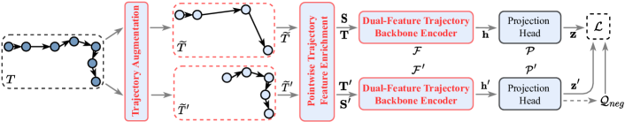
Figure 2: The model architecture of TrajCL (The modules in red are our core technical contributions.)

Model overview. Fig. 2 shows an overview of our TrajCL model. The model follows the dual-branch structure of a strong contrastive learning framework, MoCo [16]. Our technical contributions come in the design of the learning modules as highlighted in red in Fig. 2, to be detailed in the next section.

Given an input trajectory $T$, it first goes through a trajectory augmentation module to generate two different trajectory views (i.e., variants) of $T$, denoted as $\widetilde{T}$ and $\widetilde{T}^{\prime}$, respectively. We propose four different augmentation methods that emphasize different features of a trajectory (Section IV-A). The augmentation process is based on $T$ directly, and hence no additional manual data labeling efforts are needed.

The generated views $\widetilde{T}$ and $\widetilde{T}^{\prime}$ are fed into pointwise trajectory feature enrichment layers to generate pointwise features beyond just the coordinates, which reflect the key characteristics of $\widetilde{T}$ and $\widetilde{T}^{\prime}$ (Section IV-B). We represent the enriched features by two types of embeddings, the structural feature embedding and the spatial feature embedding, for each point in $\widetilde{T}$ (and $\widetilde{T}^{\prime}$). These embeddings encode pointwise structural and spatial features, and form a structural embedding matrix $\mathbf{T}$ ($\mathbf{T^{\prime}}$) and a spatial embedding matrix $\mathbf{S}$ ($\mathbf{S^{\prime}}$).

Then, we input ($\mathbf{T}$, $\mathbf{S}$) and ($\mathbf{T^{\prime}}$, $\mathbf{S^{\prime}}$) into trajectory backbone encoders $\mathcal{F}$ and $\mathcal{F}^{\prime}$ to obtain embeddings $\mathbf{h}$ and $\mathbf{h}^{\prime}$ for $\widetilde{T}$ and $\widetilde{T}^{\prime}$, respectively (Section IV-C). Our backbone encoders are adapted from Transformer [29], and they encode structural and spatial features of trajectories into the embeddings.

Next, $\mathbf{h}$ and $\mathbf{h}^{\prime}$ go through two projection heads $\mathcal{P}$ and $\mathcal{P}^{\prime}$ (which are fully connected layers of the same structure) to be mapped into lower-dimensional vectors $\mathbf{z}$ and $\mathbf{z}^{\prime}$, respectively:

$$\mathbf{z}=\mathcal{P}(\mathbf{h})=(\mathrm{FC}\circ\mathrm{ReLU}\circ\mathrm{FC})(\mathbf{h})$$ (1)

Here, $\mathrm{FC}$ denotes a fully connected layer, $\mathrm{ReLU}$ denotes the ReLU activation function, and $\circ$ denotes function composition. We omit the equation for $\mathcal{P}^{\prime}$ as it is the same. Such projections have been shown to improve the embedding quality [30, 17].

Model training. Following previous contrastive learning models, we use the InfoNCE [43] loss for model training. We use $\mathbf{z}$ and $\mathbf{z}^{\prime}$ as a pair of positive samples, as they both come from variants of $T$ and are supposed to be similar in the learned latent space. The embeddings (except $\mathbf{z}^{\prime}$) from projection head $\mathcal{P}^{\prime}$ that are in the current and recent past training batches are used as negative samples of $\mathbf{z}$. The InfoNCE loss $\mathcal{L}$ maximizes the agreement between positive samples and minimizes that between negative samples:

$$\mathcal{L}(T)=-\log\frac{\mathrm{exp}\big{(}\mathrm{sim}(\mathbf{z},\mathbf{z}^{\prime})/\tau\big{)}}{\mathrm{exp}\big{(}\mathrm{sim}(\mathbf{z},\mathbf{z}^{\prime})/\tau\big{)}+\sum_{j=1}^{|\mathcal{Q}_{neg}|}\mathrm{exp}\big{(}\mathrm{sim}(\mathbf{z},\mathbf{z}_{j}^{-})/\tau\big{)}}$$ (2)

Here, $\mathrm{sim}$ is the cosine similarity. $\tau$ is a temperature parameter that controls the contribution of the negative samples [44].

We use a queue $\mathcal{Q}_{neg}$ of a fixed size (an empirical parameter) to store negative samples. The queue includes the embeddings from $\mathcal{P}^{\prime}$ in recent batches, to enlarge the negative sample pool, since more negative samples help produce more robust embeddings [17, 16]. To reuse negative samples from recent batches, the parameters of $\mathcal{F}^{\prime}$ and $\mathcal{P}^{\prime}$ should change smoothly between batches. We follow the momentum update [16] procedure to satisfy this requirement:

$$\Theta_{\mathcal{F}^{\prime}}=m\Theta_{\mathcal{F}^{\prime}}+(1-m)\Theta_{\mathcal{F}};\ \ \ \Theta_{\mathcal{P}^{\prime}}=m\Theta_{\mathcal{P}^{\prime}}+(1-m)\Theta_{\mathcal{P}}$$ (3)

Here, $\Theta_{\mathcal{X}}$ denotes the parameters of model $\mathcal{X}$; $m\in(0,1)$ (which is 0.999 in our experiments) is a momentum coefficient that determines the smoothness of parameter updates. Note that $\Theta_{\mathcal{F}}$ and $\Theta_{\mathcal{P}}$ are still updated by stochastic gradient descent.

Once trained, the pointwise trajectory feature enrichment layers and trajectory backbone encoder $\mathcal{F}$ can be detached from TrajCL to serve as an encoder to generate embeddings for given trajectories, which can be used to directly compare the similarity between trajectories. They can also be connected to other models to approximate heuristic similarity measures.

IV Model Details

We next elaborate our model components, including trajectory augmentation methods (Section IV-A), pointwise trajectory feature enrichment layers (Section IV-B), and dual-feature self-attention-based backbone encoders (Section IV-C). We also analyze the model complexity (Section IV-D).

IV-A Trajectory Augmentation

Data augmentation creates different variants of an input record such that the encoder later can learn to capture the common (and distinguishing) features from the variants.

No augmentation methods have been proposed for trajectory contrastive learning. We propose four augmentation methods to fill this gap: (1) point shifting, (2) point masking (3) trajectory truncating, and (4) trajectory simplification. The aim is to cover the common trajectory transformations. Fig. 3 shows examples for the four methods, where the trajectory in dark blue denotes an input trajectory, and those in light blue are variants generated by the different augmentation methods.

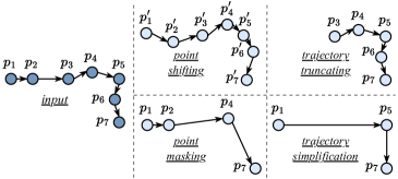
Figure 3: Examples of the proposed trajectory augmentation methods (The same $p_{i}$ on different trajectories denotes the same point from the input; $p^{\prime}_{i}$ is shifted from $p_{i}$.)

Point shifting. Given a trajectory $T$, point shifting randomly adds an offset to each coordinate of $p_{i}\in T$, aiming to learn similar trajectories with minor point location differences. The point-shifted output trajectory $\widetilde{T}$ (or $\widetilde{T}^{\prime}$, same for the rest of the subsection) of $T$ can be represented as:

$$\begin{split}\widetilde{T}=[p_{1}^{\prime},p_{2}^{\prime},\ldots,p_{|T|}^{\prime}],\mathrm{where}\;\forall p_{i}=(x_{i},y_{i})\in T,\;\;\;\\ p_{i}^{\prime}=(x_{i}+\Delta{x_{i}},y_{i}+\Delta{y_{i}}),\>\Delta{x_{i}}\sim X_{n},\>\Delta{y_{i}}\sim X_{n}\end{split}$$ (4)

Here, $\Delta{x_{i}}$ and $\Delta{y_{i}}$ are the location offsets, and $X_{n}$ is their distribution. We use a bounded Gaussian distribution $X_{n}\sim\frac{\rho_{m}}{\lambda}\cdot\mathcal{N}(\mu,{\sigma}^{2})$, since the location errors of a GPS point cannot be arbitrarily large. Parameter $\rho_{m}$ is the maximum distance offset, and $\lambda$ is a normalization coefficient to let the integral of the cumulative distribution function of $X_{n}$ to be 1: $\lambda=\int_{-{\rho_{m}}}^{{\rho_{m}}}f_{X_{n}}(x)dx$, where $f_{X_{n}}(x)$ is the probability density function of $X_{n}$. We set $\rho_{m}$ at 100 meters and use $\mathcal{N}(0,0.5^{2})$ in the experiments.

Point masking. Given a trajectory $T$, point masking randomly masks (i.e., removes) a subset of points in $T$ to generate a variant $\widetilde{T}$, to help learn similar trajectories with varying sampling rates or incomplete records. We use an independent and identically uniform distribution for the masking probability of each point, and we set the proportion of points masked, $\rho_{d}\in(0,1)$, to 0.3 in our experiments. The point-masked output trajectory $\widetilde{T}$ is represented as:

$$\begin{split}\widetilde{T}\;=\;[p_{n_{1}},p_{n_{2}},\ldots,p_{n_{|\widetilde{T}|}}],\end{split}$$ (5)

where $n_{1},n_{2},\ldots,n_{|\widetilde{T}|}$ is a strictly increasing sequence, $\widetilde{T}\subset T$, and ${|\widetilde{T}|}=\lfloor(1-\rho_{d})\cdot|T|\rfloor$.

Trajectory truncating. Given a trajectory $T$, trajectory truncating cuts a prefix or a suffix (or both) from $T$ and keeps the rest as a variant $\widetilde{T}$. This method aims to uncover partially overlapped trajectories for applications such as carpooling. We use a parameter $\rho_{b}\in(0,1)$ to control the proportion of points kept in $\widetilde{T}$. We set $\rho_{b}=0.7$ in the experiments. Formally, a variant $\widetilde{T}$ generated by trajectory truncating is represented as:

$$\begin{split}\widetilde{T}=&[p_{i},p_{i+1},\ldots,p_{\lfloor i+\rho_{b}\cdot|T|\rfloor}],\;\\ &\text{where }i\text{ is a random integer in }[1,\lceil(1-\rho_{b})\cdot|T|\rceil]\end{split}$$ (6)

Trajectory simplification. Given a trajectory $T$, trajectory simplification removes points from $T$ that are not critical to the overall shape and trend of $T$ to form a variant $\widetilde{T}$. The variant is meant to guide the trajectory encoder to focus on the critical (e.g., turning) points of $T$. We adopt the Douglas–Peucker (DP) simplification algorithm [45] for its wide applicability, although other simplification methods also apply. DP starts by drawing a line segment to connect the two end points of $T$. The breaking point of $T$ that is the farthest from this line segment is calculated (e.g., $p_{5}$ in Fig. 3), and two line segments are drawn to connect this point with the two initial end points, respectively. We repeat the breaking point finding process on each of the two line segments recursively, until the breaking points found are close to the line segments enough (defined by a threshold $\rho_{p}$ which is 100 meters in the experiments). Only the breaking points found in the process are kept in $\widetilde{T}$.

$$\widetilde{T}=\text{Douglas\_Peucker}(T)$$ (7)

Discussion. Parameters $\rho_{m}$, $\rho_{d}$, $\rho_{b}$ and $\rho_{p}$ above control how far off an augmented trajectory can be from the input trajectory. We have set empirical values for them, while changing their values offers flexibility in creating augmented trajectories that help learn embeddings for trajectory similarity queries of different accuracy requirements.

IV-B Pointwise Trajectory Feature Enrichment

After augmenting $T$, we obtain two augmented trajectory views $\widetilde{T}$ and $\widetilde{T}^{\prime}$. The next step is to enrich $\widetilde{T}$ and $\widetilde{T}^{\prime}$ to create features beyond just point coordinates that can reflect the key characteristics of trajectories, which will later be used as the input to the trajectory backbone encoder.

We create two types of features, i.e., structural features and spatial features, for every trajectory point, and we represent each feature by an embedding vector, i.e., the structural feature embedding and the spatial feature embedding. To also preserve the relative position information of the points, we further encode positional information into embedding vectors.

Structural feature embedding. The structural features aim to capture the general shape and point connectivity of a trajectory. We partition the data space with a regular grid where the cell side length is a system parameter, and we represent a trajectory point by the grid cell enclosing it. The sequence of grid cells passed by a trajectory $\widetilde{T}$ (or $\widetilde{T}^{\prime}$) depicts the trajectory shape, and the cell adjacency relationships reflect the connectivity among the points on the trajectory.

Using an ID to represent each cell (and the trajectory points inside) offers only sparse information and misses the cell adjacency relationships. Instead, we learn a cell embedding to capture such information as follows. We construct a graph where each vertex represents a grid cell. A vertex corresponding to a cell is connected by an edge to each of the eight vertices that correspond to the eight cells surrounding the given cell. We then run a self-supervised graph embedding algorithm (i.e., node2vec [46]) to learn the vertex embeddings which encode the graph (and hence the grid) structural information. The vertex embeddings are used as the cell embeddings.

Once the cell embeddings (of $d_{t}$ dimensions) are obtained, we represent every point $p_{i}$ on $\widetilde{T}$ (and $\widetilde{T}^{\prime}$) by the cell embedding of $p_{i}$. This results in an embedding matrix $\mathbf{T}\in\mathbb{R}^{|\widetilde{T}|\times d_{t}}$ (and $\mathbf{T^{\prime}}\in\mathbb{R}^{|\widetilde{T}^{\prime}|\times d_{t}}$) to represent $\widetilde{T}$ (and $\widetilde{T}^{\prime}$).

Spatial feature embedding. We further capture fine-grain location information of the points in a trajectory by computing their spatial feature embeddings.

Given a point $p_{i}$ on $\widetilde{T}$ (or $\widetilde{T}^{\prime}$), its spatial feature embedding is a four-tuple $(x_{i},y_{i},r_{i},l_{i})$, where $x_{i}$ and $y_{i}$ are its spatial coordinates, $r_{i}$ is the radian between the two trajectory segments before and after $p_{i}$, i.e., $\overline{p_{i-1},p_{i}}$ and $\overline{p_{i},p_{i+1}}$, respectively, and $l_{i}$ is the mean length of $\overline{p_{i-1},p_{i}}$ and $\overline{p_{i},p_{i+1}}$. Formally:

$$r_{i}=\angle p_{i-1}p_{i}p_{i+1};\quad\quad l_{i}=0.5\times\big{(}|\overline{p_{i-1},p_{i}}|+|\overline{p_{i},p_{i+1}}|\big{)}$$ (8)

We use $\mathbf{S}\in\mathbb{R}^{|\widetilde{T}|\times d_{s}}$ and $\mathbf{S^{\prime}}\in\mathbb{R}^{|\widetilde{T}^{\prime}|\times d_{s}}$ to denote the spatial feature embedding matrices of $\widetilde{T}$ and $\widetilde{T}^{\prime}$, respectively ($d_{s}=4$).

Position encoding. The structural and the spatial feature embeddings have not considered the relative positions (i.e., preceding and subsequent) of the points on a trajectory, which are important information in trajectory similarity. We modify these embeddings to further encode such information.

We adopt the sine and cosine functions [29] for point-in-sequence position encoding. For the $j$-th dimension value of the structural feature embedding (and the spatial feature embedding) of the $i$-th point on a trajectory, denoted by $\mathbf{T}[i,j]$ (and $\mathbf{S}[i,j]$), we update it by adding the following value $e_{i,j}$:

$$\begin{split}&\mathbf{T}[i,j]=\mathbf{T}[i,j]+e_{i,j};\quad\quad\mathbf{S}[i,j]=\mathbf{S}[i,j]+e_{i,j}\\ e_{i,j}&=\begin{cases}\>\sin\big{(}i/10000^{j/d_{p}}\big{)},&j\text{ is even}\\ \>\cos\big{(}i/10000^{(j-1)/d_{p}}\big{)},&j\text{ is odd}\end{cases}\end{split}$$ (9)

Here, $d_{p}$ denotes the embedding dimensionality of $T$ or $S$, respectively. Intuitively, $e_{i,j}$ encodes the position information $i$ which is added to the embeddings of the $i$-th point.

IV-C Dual-Feature Self-Attention-Based Backbone Encoder

We propose a dual-feature self-attention-based trajectory backbone encoder (DualSTB) equipped with a dual-feature multi-head self-attention module (DualMSM) to capture both structural and spatial features of an input trajectory. Compared with the vanilla multi-head self-attention module (MSM) in Transformer [29], DualMSM models not only attentions for each type of features separately but also their joint impact, to generate more comprehensive trajectory representations.

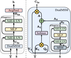
Figure 4: The dual-feature self-attention-based trajectory backbone encoder, DualSTB (left), and the dual-feature multi-head self-attention module, DualMSM (right)

DualSTB. Fig. 4 shows the structure of DualSTB (the left sub-figure) and its DualMSM module (the right sub-figure). DualSTB follows the overall structure of a multi-layer Transformer encoder, where our new design lies in DualMSM and the use of two types of input $\mathbf{T}$ and $\mathbf{S}$ instead of one ($\mathbf{T^{\prime}}$ and $\mathbf{S^{\prime}}$ for DualSTB over $\widetilde{T^{\prime}}$, which is omitted below for conciseness). We include the computation steps of the DualSTB encoder for completeness. Readers who are familiar with the Transformer model can skip the next paragraph.

DualSTB takes $\mathbf{T}$ and $\mathbf{S}$ as the input, which go through a DualMSM module to learn the joint attention of the input features. The output of DualMSM, denoted by $\mathbf{C_{ts}}$, is fed to a residual connection [47] (i.e., a dropout function [48] and an add function) and a layer normalization [49] which help alleviate the problems of gradient vanishing and explosion to obtain smoother gradients. Then, the output goes through a multi-layer perceptron (MLP) with a residual connection and a layer normalization to slow down the model degeneration. The post-DualMSM processing steps are summarized as follows:

$$\hat{\mathbf{C}}_{\mathbf{ts}}=\mathrm{LayerNorm}(\mathbf{T}+\mathrm{Dropout}(\mathbf{C}_{\mathbf{ts}}))$$ (10)

$$\mathbf{H}_{\mathbf{ts}}=\mathrm{LayerNorm}(\hat{\mathbf{C}}_{\mathbf{ts}}+\mathrm{Dropout}(\mathrm{MLP}(\hat{\mathbf{C}}_{\mathbf{ts}})))$$ (11)

Here, $\hat{\mathbf{C}}_{\mathbf{ts}}$ is an intermediate result and $\mathbf{H}_{\mathbf{ts}}$ is the trajectory point representation matrix based on both structural and spatial features. Multiple layers (two in the experiments) of the structures are stacked. Finally, we apply average pooling on $\mathbf{H}_{\mathbf{t}\mathbf{s}}$ of the last layer to obtain trajectory representation $\mathbf{h}\in\mathbb{R}^{d}$, by averaging along each dimension of the point representations.

DualMSM. The core learning module of the DualSTB encoder, DualMSM, takes as input both structural features $\mathbf{T}\in\mathbb{R}^{l\times d_{t}}$ and spatial features $\mathbf{S}\in\mathbb{R}^{l\times d_{s}}$ of a trajectory and outputs the hidden representations of trajectory points. Here, $l$ denotes the maximum number of points on a trajectory. We pad trajectories with less than $l$ points with 0’s.

DualMSM first applies linear transformations on $\mathbf{T}$ to obtain a value matrix $\mathbf{V}_{\mathbf{t}}^{i}\in\mathbb{R}^{l\times(d_{t}/h)}=\mathbf{T}\mathbf{W}_{v}^{i}$, a key matrix $\mathbf{K}_{\mathbf{t}}^{i}\in\mathbb{R}^{l\times(d_{t}/h)}=\mathbf{T}\mathbf{W}_{k}^{i}$ and a query matrix $\mathbf{Q}_{\mathbf{t}}^{i}\in\mathbb{R}^{l\times(d_{t}/h)}=\mathbf{T}\mathbf{W}_{q}^{i}$, where $h$ is the number of heads, $i$ denotes the $i$-th head, and $\mathbf{W}_{v}^{i}$, $\mathbf{W}_{k}^{i}$ and $\mathbf{W}_{q}^{i}$ (all in $\mathbb{R}^{d_{t}\times(d_{t}/h)}$) are learnable weights of the $i$-th head. The multi-head mechanism maps different features of $\mathbf{T}$ into different feature sub-spaces such that each head only needs to focus on part of the features. Each single head attention still covers all features of $\mathbf{T}$, to reduce feature bias. Besides, the linear transformation strengthens the representation capacity of the inputs and refrains the attention coefficient matrix from degrading into an identity matrix.

Then, we compute the attention coefficients between the input points of each trajectory:

$$\mathbf{A}_{\mathbf{t}}^{i}=\mathrm{Softmax}\big{(}\frac{\mathbf{Q}_{\mathbf{t}}^{i}\mathbf{K}_{\mathbf{t}}^{{i}\mathsf{T}}}{\sqrt{d_{t}/h}}\big{)}$$ (12)

Here, $\sqrt{d_{t}/h}$ is used as a scaling factor, and $\mathbf{A}_{\mathbf{t}}^{i}$ is the structural attention coefficient matrix of the $i$-th head, which represents the structural correlation between the points (cf. the left half of the DualMSM module in Fig. 4).

For the right half of DualMSM in Fig. 4, following a procedure similar to the above, we compute $\mathbf{V}_{\mathbf{s}}^{i}$, $\mathbf{K}_{\mathbf{s}}^{i}$ and $\mathbf{Q}_{\mathbf{s}}^{i}$ based on the spatial features $\mathbf{S}$ with a different set of learnable parameters, and we compute the spatial attention coefficient matrices $\mathbf{A}_{\mathbf{s}}^{i}$ following an equation like Equation 12.

Then, we multiply the spatial attention coefficient matrix $\mathbf{A}_{\mathbf{s}}^{i}$ with the value matrix $\mathbf{V}_{\mathbf{s}}^{i}$ to obtain the hidden output $\mathbf{C}_{\mathbf{s}}^{i}\in\mathbb{R}^{l\times(d_{s}/h)}$ for input $\mathbf{S}$ on the $i$-th head:

$$\mathbf{C}_{\mathbf{s}}^{i}=\mathbf{A}_{\mathbf{s}}^{i}\times\mathbf{V}_{\mathbf{s}}^{i}$$ (13)

After that, we concatenate the output of each head to form the full hidden output $\mathbf{C}_{\mathbf{s}}$ for $\mathbf{S}$:

$$\mathbf{C}_{\mathbf{s}}=(\mathbf{C}_{\mathbf{s}}^{1}\|\mathbf{C}_{\mathbf{s}}^{2}\|\mathbf{C}_{\mathbf{s}}^{3}\;...\;\|\mathbf{C}_{\mathbf{s}}^{h})\mathbf{W}_{o}$$ (14)

where $\|$ denotes concatenation, and $\mathbf{W}_{o}\in\mathbb{R}^{d_{s}\times d_{s}}$ is the learnable weight matrix. The steps above on $\mathbf{S}$ correspond to the MSM module at the bottom right of Fig. 4.

The full hidden output $\mathbf{C}_{\mathbf{s}}$ then goes through layer normalization with a residual connection, an MLP module with a residual connection, and another layer normalization like those described by Equations 10 and 11 above, where $\hat{\mathbf{C}}_{\mathbf{ts}}$, $\mathbf{T}$, $\mathbf{C}_{\mathbf{ts}}$ and $\mathbf{H}_{\mathbf{ts}}$ are replaced by $\hat{\mathbf{C}}_{\mathbf{s}}$, $\mathbf{S}$, $\mathbf{C}_{\mathbf{s}}$ and $\mathbf{H}_{\mathbf{s}}$, respectively. Similar to Transformer, we stack these layers in DualMSM (two layers in the experiments).

So far, we have obtained both the structural and the spatial attention coefficient matrices $\mathbf{A}_{\mathbf{t}}^{i}$ and $\mathbf{A}_{\mathbf{s}}^{i}$ ($\mathbf{A}_{\mathbf{s}}^{i}$ denotes the matrix of the last stacked layer). We calculate a weighted sum of $\mathbf{A}_{\mathbf{t}}^{i}$ and $\mathbf{A}_{\mathbf{s}}^{i}$ with a learnable weighting parameter $\gamma$ as the final attention coefficient. This learnable parameter guides the learned embeddings to adaptively take structural and spatial correlations between trajectory points into consideration. The output of the $i$-th head of DualMSM, denoted as $\mathbf{C}_{\mathbf{t}\mathbf{s}}^{i}\in\mathbb{R}^{l\times(d_{t}/h)}$, is computed by:

$$\mathbf{C}_{\mathbf{t}\mathbf{s}}^{i}=\big{(}\mathbf{A}_{\mathbf{t}}^{i}+\gamma\mathbf{A}_{\mathbf{s}}^{i})\mathbf{V}_{\mathbf{t}}^{i}$$ (15)

Lastly, similar to $\mathbf{C}_{\mathbf{s}}^{i}$ in Equation 14, we concatenate the output of each head $\mathbf{C}_{\mathbf{t}\mathbf{s}}^{i}$ and apply a linear transformation to form the final output of DualMSM, i.e., $\mathbf{C}_{\mathbf{t}\mathbf{s}}\in\mathbb{R}^{l\times d_{t}}$.

Discussion. The differences between DualMSM and the vanilla MSM [29] are twofold. First, DualMSM takes as input two types of features, i.e., structural and spatial, for trajectory embedding learning, while MSM only accepts one type of input features. One may concatenate both types of features into one to suit the input structure of MSM. Such an approach, however, is shown to be inferior empirically (Section V-G). Second, DualMSM allows learning exclusive attention coefficients for each type of input features, which are then integrated adaptively. Such a mechanism is not supported in MSM. This mechanism ensures that the correlations (i.e., the attention coefficients) between points based on different types of features are modeled independently, while the adaptive integration makes the attention mechanism more flexible to combine different types of input features.

IV-D Cost Analysis

TrajCL takes $O(l^{2}\cdot d\cdot L)$ time to compute $\mathbf{h}$ for $T$, where $l$ denotes the number of points on $T$, and $L$ is the number of DualMSM layers. This cost has hidden the $O(l)$ time to obtain the pointwise trajectory features, i.e., $T\rightarrow\mathbf{T}$ and $\mathbf{S}$, since the dominating cost comes from the trajectory encoding stage (i.e., $\mathbf{T}$ and $\mathbf{S}\rightarrow\mathbf{h}$), in particular, the matrix multiplication costs in Equations 12 and 13. Without any recurrent structures, our TrajCL model can be easily accelerated by GPUs.

In comparison, the representative competitor methods t2vec [11] and E2DTC [14] take $O(l\cdot d^{2}\cdot L)$ time to compute a trajectory embedding, TrjSR [12] takes $O(m^{2}\cdot k^{2}\cdot n_{k}\cdot cl\cdot L)$ time, and CSTRM [13] takes the same time as TrajCL, where $m$ is the side length (number of pixels) of trajectory images, $k$ is the side length of convolution kernels, $n_{k}$ is the number of kernels, and $cl$ is the number of image channels in TrjSR.

Once $\mathbf{h}$ is obtained, it will only take a time linear to $d$ to compute the similarity between two trajectories.

V Experiments

We evaluate TrajCL on four real trajectory datasets by comparing with heuristic methods and learned methods for both trajectory similarity computation and similarity queries. We also study the effectiveness of TrajCL on a downstream task by fine-tuning it to learn heuristic similarity measures. Finally, we study the impact of model components and parameters.

V-A Experimental Settings

Datasets. We use four real-world trajectory datasets: (1) Porto [15] contains 1.7 million taxi trajectories from Porto, Portugal, between July 2013 and June 2014; (2) Chengdu [50], contains 6.1 million ride-hailing trajectories from Chengdu, China, during November 2016; (3) Xi’an [50] contains 2.1 million ride-hailing trajectories from Xi’an, China, during the first two weeks of October 2018; and (4) Germany [51] is a country-wide dataset, containing 170.7 thousand user-submitted trajectories within Germany, between 2006 and 2013. Following previous studies [11, 12, 13], we preprocess each dataset by filtering out trajectories that are outside the city area or contain less than 20 points or more than 200 points. The datasets after preprocessing are summarized in Table II.

TABLE II: Dataset statistics

3	Porto	Chengdu	Xi’an	Germany
#trajectories	1,372,725	4,477,858	900,562	143,417
Avg. #points per trajectory	48	105	118	72
Max. #points per trajectory	200	200	200	200
Avg. trajectory length (km)	6.37	3.47	3.25	252.49
Max. trajectory length (km)	80.61	23.12	99.41	115,740.67
3

Each dataset is randomly partitioned into four disjoint subsets: (1) 200,000 trajectories in Porto, Chengdu and Xi’an, and 30,000 trajectories in Germany for training, respectively, (2) a 10% subset for validation, (3) 100,000 trajectories for testing, and (4) 10,000 trajectories for downstream task experiments, i.e., learning to approximate a heuristic similarity measure, which are further split by 7:1:2 for training, validation, and testing.

Competitors. We compare our method TrajCL with four representative heuristic trajectory similarity measures, i.e., EDR [7], EDwP [8], Hausdorff [9] and Fréchet [10], and three recently proposed self-supervised learned measures, i.e., t2vec [11], TrjSR [12], E2DTC [14] and CSTRM [13] Similar to TrajCL, all these measures are used as a standalone trajectory similarity measure. These baseline methods are described in Section II.

In the downstream task, i.e., fine-tuning TrajCL to learn and approximate a heuristic measure, we compare TrajCL with the above self-supervised learned methods, as well as the latest supervised methods Traj2SimVec [19], T3S [20] and TrajGAT [21]. We omit NEUTRAJ [18] as it has been shown to be outperformed by these methods already.

We use the released code and default parameters for all baseline methods except Traj2SimVec and T3S which have no released code. We implement these two methods following their original proposals [19, 20].

Implementation details. We implement TrajCL with PyTorch 1.8.1. We run experiments on a machine with a 32-core Intel Xeon CPU, an NVIDIA Tesla V100 GPU and 64 GB RAM. We report mean results over five runs of each experiment with different random seeds.

We train TrajCL using the Adam optimizer. The maximum number of training epochs is set to 20, and we early stop after 5 consecutive epochs without improvements in the loss. The learning rate is initialized to 0.001 and decayed by half after every 5 epochs. We set the embedding dimensionality $d$ to 256 for all learned methods except TrajGAT, which performs better with its default $d$ value 32 and hence has used this value. For TrajCL and T3S, the number of heads $h$ is 4, and the number of encoder layers $\#layers$ is 2. The default augmentation methods are point masking and trajectory truncating for the two views. The side length of the grid cells is 100 meters.

We use ‘$\blacktriangle$’ (and ‘$\blacktriangledown$’) to indicate that larger (and smaller) values are better, and the best results are in bold.

V-B Learning Trajectory Similarity

We first investigate the effectiveness of TrajCL on learning trajectory similarity, i.e., to find similar trajectories.

Setup. Following the baseline methods [11, 12, 13], the experimental data includes a query set $Q$ and a database $D$, which are created from the 100,000 randomly chosen testing set (see Datasets in Section V-A above) as follows. We test how well TrajCL can help recover the ground-truth similar trajectories in $D$ for the query trajectories in $Q$.

From each dataset, we randomly sample 1,000 trajectories from the 100,000 testing set. For each sampled trajectory $T^{q}$, we create two sub-trajectories – one consisting of the odd points of $T^{q}$, i.e., $T^{q}_{a}=[p_{1},p_{3},p_{5},\ldots]$, and the other the even points, i.e., $T^{q}_{b}=[p_{2},p_{4},p_{6},\ldots]$. Trajectory $T^{q}_{a}$ is put into the query set $Q$, and $T^{q}_{b}$ is put into the database $D$ and will serve as the ground-truth most similar trajectory of $T^{q}_{a}$. We further add randomly chosen trajectories from the testing set into $D$ to form databases of different sizes. We generate $T^{q}_{a}$ and $T^{q}_{b}$ because there is no known ground-truth similar trajectory pair. Such a pair can be seen as different trajectories recorded with the same sampling rate for the same movement sequence but starting at slightly different locations. Thus, they can be considered as a reasonably similar pair.

For every query $T^{q}_{a}\in Q$, we compute the similarity between $T^{q}_{a}$ and all trajectories in $D$ (for each method), and we report the mean rank of $T^{q}_{b}$ by sorting the similarity values of trajectory pairs in descending order. Ideally, $T^{q}_{b}$ should rank 1^st, for the reason above.

TABLE III: Mean rank ($\blacktriangledown$) of the ground truth most similar trajectory vs. database size (Best results are in bold.)

3 Dataset	Method	20K	40K	60K	80K	100K
Porto	EDR	8.318	14.398	17.983	22.902	28.753
	EDwP	3.280	4.579	5.276	6.191	7.346
	Hausdorff	3.068	4.014	4.649	5.451	6.376
	Fréchet	3.560	4.959	5.968	7.192	8.631
	t2vec	1.523	2.051	2.257	2.612	3.068
	TrjSR	1.876	2.783	3.208	3.826	4.635
	E2DTC	1.560	2.111	2.349	2.731	3.213
	CSTRM	4.476	7.954	10.630	13.576	16.699
	TrajCL	1.005	1.006	1.006	1.007	1.010
Chengdu	EDR	80.021	156.847	234.128	312.528	388.796
	EDwP	9.066	15.890	22.779	29.615	36.724
	Hausdorff	25.248	48.293	71.537	94.861	118.179
	Fréchet	18.973	35.731	52.622	69.617	86.620
	t2vec	4.705	8.225	11.811	15.461	19.114
	TrjSR	4.421	7.723	11.027	14.364	17.873
	E2DTC	5.062	8.880	12.816	16.784	20.775
	CSTRM	5.914	10.655	15.423	20.100	24.900
	TrajCL	1.038	1.074	1.113	1.151	1.200
Xi’an	EDR	57.149	113.583	169.284	224.900	280.126
	EDwP	2.318	2.611	2.929	3.288	3.606
	Hausdorff	37.896	74.044	109.996	145.924	182.224
	Fréchet	40.378	79.087	117.677	156.159	194.685
	t2vec	2.574	4.047	5.538	7.047	8.644
	TrjSR	13.791	26.901	39.683	52.559	65.647
	E2DTC	2.988	4.909	6.854	8.810	10.861
	CSTRM	3.078	5.231	7.317	9.402	11.635
	TrajCL	1.023	1.050	1.066	1.087	1.107
Germany	EDR	279.385	558.288	834.208	1108.975	1370.004
	EDwP	2.168	2.277	2.371	2.454	2.515
	Hausdorff	2.803	3.509	4.206	4.906	5.551
	Fréchet	2.581	3.108	3.633	4.113	4.589
	t2vec	1.571	1.982	2.387	2.718	3.053
	TrjSR	6.517	11.741	16.969	22.182	24.083
	E2DTC	3.136	5.156	7.248	9.207	10.956
	CSTRM	-	-	-	-	-
	TrajCL	1.012	1.022	1.034	1.040	1.045
3

Results. Varying database size $|D|$. We first vary the database size $|D|$ from 20,000 to 100,000. Table III shows the mean rank of $T^{q}_{b}$ (smaller values are better) produced by the different methods. TrajCL outperforms all heuristic and learned similarity measures on all four datasets, producing mean ranks very close to 1 consistently. For example, on Porto, compared with those of the best heuristic competitor Hausdorff and the best learned competitor t2vec, the mean rank of $T^{q}_{b}$ for TrajCL is up to 5.31 times and 2.04 times smaller (1.010 vs. 6.376 and 3.068 when $|D|$=100K), respectively. Further, TrajCL shows better stability with respect to $|D|$. When $|D|$ grows, TrajCL  can still tell that $T^{q}_{b}$ is more similar to $T^{q}_{a}$ than any other trajectories added to $D$, with the worst mean rank of $T^{q}_{b}$ being 1.200, which is captured on Chengdu when $|D|$=100K. In comparison, the worst-case mean rank of $T^{q}_{b}$ of the best baseline method (i.e., TrjSR) on the same dataset grows to 17.873 which is 13.89 times larger. Such results confirm the effectiveness of TrajCL to obtain better trajectory representations that preserve the similarity.

We note that t2vec and E2DTC share similar results, as they use the same backbone encoder. E2DTC is slightly worse than t2vec even though it is a newer method. This is because E2DTC is designed for trajectory clustering which may not be optimized for trajectory similarity learning. We also note that TrjSR has reported better performance than t2vec [12]. However, we were not able to produce the same results on our datasets, while we do not have access to their datasets.

Besides, although CSTRM also uses self-attention, it cannot accurately learn trajectory similarity. This is because CSTRM uses the vanilla MSM and only learns coarse-grained trajectory representations based on grid cells, while our proposed DualMSM can capture both coarse-grained and fine-grained features and leverage the topology of grid cells. Further, due to the large number of parameters of the cell embedding module in CSTRM, it triggers an out-of-memory error on Germany and hence no results were obtained.

Further, we observe that, in general, the learning-based methods achieve better results on Germany than on Chengdu and Xi’an, and best results on Porto. Germany has the largest geographical region and grid space among the four datasets, while it has the fewest training trajectories. These make trajectory point correlation learning among different grid cells difficult and lead to a more challenging dataset than Porto. On the other hand, Germany has the lowest trajectory density, and its trajectories are easier to be distinguished among each other, especially comparing with those in the Chengdu and Xi’an datasets which are much denser (with the smaller spatial regions).

Varying down-sampling rate $\rho_{s}$. We down-sample trajectories in $Q$ and $D$ by randomly masking points in each trajectory with a probability $\rho_{s}\in[0.1,0.5]$, while $|D|=100,000$. Table IV shows the performance results. TrajCL again achieves the smallest mean ranks of $T^{q}_{b}$ consistently. Compared with the best heuristic competitor EDwP and the best learned competitor t2vec, TrajCL reduces the mean rank of $T^{q}_{b}$ by at least 0.87 times and 2.17 times (on Porto), while the advantage is up to 11.38 times and 12.01 times, respectively.

TABLE IV: Mean rank ($\blacktriangledown$) vs. down-sampling rate

3 Dataset	Method	0.1	0.2	0.3	0.4	0.5
Porto	EDR	57.173	203.993	806.033	2286.821	4872.231
	EDwP	8.442	10.968	18.727	28.394	68.061
	Hausdorff	10.026	23.293	56.561	89.827	275.206
	Fréchet	10.668	18.516	29.740	93.851	181.271
	t2vec	4.786	8.461	19.689	35.219	115.364
	TrjSR	7.941	15.746	151.948	549.108	1341.883
	E2DTC	5.100	9.385	21.845	39.402	124.320
	CSTRM	24.794	47.137	123.124	257.540	687.262
	TrajCL	1.026	1.191	1.513	3.847	36.352
Chengdu	EDR	398.870	455.498	446.041	594.004	820.628
	EDwP	35.954	35.553	34.232	38.848	41.424
	Hausdorff	117.908	121.474	116.300	125.098	152.359
	Fréchet	87.673	89.005	86.420	91.204	104.220
	t2vec	19.539	20.168	20.037	23.662	30.864
	TrjSR	20.193	27.302	57.337	88.716	111.768
	E2DTC	21.247	21.936	21.515	25.387	35.381
	CSTRM	30.165	34.347	41.677	53.707	75.486
	TrajCL	1.219	1.465	1.261	6.611	15.523
Xi’an	EDR	279.835	285.550	340.820	367.227	516.571
	EDwP	4.038	7.047	10.499	20.807	25.631
	Hausdorff	64.390	122.651	124.112	127.969	184.158
	Fréchet	66.813	86.647	144.120	160.499	196.099
	t2vec	9.929	10.710	15.098	22.184	22.493
	TrjSR	85.815	114.777	140.970	147.401	336.613
	E2DTC	12.411	11.918	26.242	18.267	28.326
	CSTRM	13.153	16.056	25.374	34.194	47.146
	TrajCL	1.198	1.371	1.414	2.162	2.446
Germany	EDR	1368.829	1379.489	1375.261	1380.517	1389.433
	EDwP	2.173	2.509	2.176	2.191	2.209
	Hausdorff	2.514	2.742	4.353	4.448	5.627
	Fréchet	2.358	2.492	3.735	3.824	4.642
	t2vec	4.453	6.736	9.087	9.470	9.775
	TrjSR	24.539	30.318	55.002	68.070	111.175
	E2DTC	11.595	13.478	15.843	18.532	19.134
	CSTRM	-	-	-	-	-
	TrajCL	1.048	1.050	1.059	1.418	2.045
3

TABLE V: Mean rank ($\blacktriangledown$) vs. distortion rate

3 Dataset	Method	0.1	0.2	0.3	0.4	0.5
Porto	EDR	28.243	28.498	27.899	28.070	28.932
	EDwP	7.591	7.166	7.038	7.235	7.236
	Hausdorff	6.549	6.737	6.706	6.592	6.739
	Fréchet	8.689	8.854	8.755	8.636	9.083
	t2vec	3.212	3.487	3.981	3.897	3.999
	TrjSR	4.781	5.087	35.144	6.194	7.201
	E2DTC	3.348	3.678	4.210	4.129	4.222
	CSTRM	20.860	20.081	22.081	24.688	26.243
	TrajCL	1.022	1.154	1.076	1.091	1.039
Chengdu	EDR	381.155	374.169	368.976	364.785	360.5494
	EDwP	34.392	33.151	33.817	29.300	29.193
	Hausdorff	117.189	116.779	117.954	116.999	117.850
	Fréchet	86.658	86.949	88.367	88.238	88.253
	t2vec	19.263	16.919	19.262	19.044	19.436
	TrjSR	21.408	22.898	54.451	20.376	24.377
	E2DTC	20.627	18.012	20.629	20.705	20.758
	CSTRM	25.026	27.530	28.691	29.349	26.786
	TrajCL	1.168	1.260	1.810	2.508	1.115
Xi’an	EDR	275.205	270.394	266.143	263.054	259.541
	EDwP	16.545	7.587	16.371	17.833	35.977
	Hausdorff	184.629	183.114	188.238	186.298	179.990
	Fréchet	195.383	195.244	195.385	197.348	196.140
	t2vec	11.045	11.912	10.522	12.834	12.233
	TrjSR	64.139	82.476	89.274	106.198	80.282
	E2DTC	13.490	14.768	13.227	16.621	16.498
	CSTRM	15.261	15.063	13.253	16.865	13.924
	TrajCL	1.331	1.376	1.420	1.470	1.268
Germany	EDR	1373.985	1372.984	1373.981	1373.966	1373.944
	EDwP	2.488	2.489	2.492	2.489	2.489
	Hausdorff	5.587	5.576	5.573	5.566	5.568
	Fréchet	4.631	4.625	4.609	4.625	4.612
	t2vec	3.863	3.976	4.903	3.580	3.625
	TrjSR	27.146	27.156	27.032	26.935	27.035
	E2DTC	10.946	11.161	10.940	11.275	10.693
	CSTRM	-	-	-	-	-
	TrajCL	1.049	1.051	1.049	1.062	1.054
3

Varying distortion rate $\rho_{d}$. We further randomly distort the trajectories in $Q$ and $D$ by shifting point coordinates following Equation 4. We vary the proportion of points distorted in each trajectory, denoted by $\rho_{d}$, from 0.1 to 0.5, and we keep $|D|=100,000$. Table V shows the results, where TrajCL outperforms all competitors again. Compared with the best baseline t2vec, TrajCL reduces that mean rank of $T^{Q}_{b}$ by up to 2.85, 16.43, 27.37 and 3.67 times on the Porto, Chengdu, Xi’an and Germany datasets, respectively. The results further confirm that TrajCL is more robust than the competitors on trajectories with distorted points. We observe that the results of all methods may fluctuate when $\rho_{d}$ varies. This is because the random distortion is applied to all trajectories, not just the query or ground-truth ones. The relative similarity of the different trajectories may change towards any direction, such that there is no unified changing pattern of the mean rank of the target trajectory.

TABLE VI: Mean rank ($\blacktriangledown$) vs. test dataset

3					$\mathbf{|D|}$=100K	$\mathbf{\rho_{s}}$=0.2	$\mathbf{\rho_{d}}$=0.2
Xi’an $\rightarrow$ Xi’an	t2vec	8.644	10.710	11.912
	TrajCL	1.107	1.371	1.376
Porto $\rightarrow$ Xi’an	t2vec	1021.883	1031.330	6430.850
	TrajCL	4.211	8.295	10.682
3

Varying test dataset. We further study the generalizability of TrajCL under a cross-dataset setting, i.e., training TrajCL on Porto and testing it on Xi’an without fine-tuning (denoted as Porto $\rightarrow$ Xi’an). We compare with the best learned competitor, t2vec, and we report the mean ranks of $T^{q}_{b}$ for the representative settings where $|D|$=100K (no trajectory modification), $\rho_{s}$=0.2 and $\rho_{d}$=0.2, respectively. We only present the results on Porto, since the relative performance on the other datasets is similar. We also contrast the results with those on model training and testing both on Xi’an (denoted as Xi’an $\rightarrow$ Xi’an).

As Table V-B shows, TrajCL consistently outperforms t2vec under the cross-dataset setting, and the performance gap is even larger than that under the same-dataset setting. Comparing with the results reported in Tables III, IV and V on Xi’an, TrajCL (Porto $\rightarrow$ Xi’an) still outperforms most of the heuristic methods which are dataset independent, except for EDwP with a small gap (4.211 vs. 3.606 at $|D|=100K$). These results show the strong generalizability of TrajCL, attributing to our dual-feature encoder which can capture generic correlation patterns between similar trajectories that translate across datasets. In comparison, t2vec uses $k$NN to compute the distance between cells, which is more vulnerable to a changed data distribution across datasets.

V-C Efficiency of Similarity Computation

Setup. We report the training and testing times of the different methods to compute the similarity between 1,000 query trajectories from $Q$ against 100,000 data trajectories in $D$, i.e., $10^{8}$ trajectory similarity computations in total. The heuristic methods are run on a 32-core CPU. The learning-based methods are trained on GPU, and tested on a 32-core CPU and on GPU (to observe the best performance) separately.

TABLE VII: Training time of learning-based measures (second)

3	Porto	Chengdu	Xi’an	Germany
t2vec	5,992	6,599	6,638	852
TrjSR	31,983	32,088	32,137	9,604
E2DTC	7,998	8,893	9,759	1,856
CSTRM	2,956	3,070	3,650	-
TrajCL	3,611	3,572	4,182	524
3

TABLE VIII: Trajectory similarity computation times (second)

3		Porto	Chengdu	Xi’an	Germany
CPU only	EDR	734	2,007	3,451	4,609
	EDwP	31,956	180,381	305,219	341,904
	Hausdorff	663	1,244	1,911	3,568
	Fréchet	1,047	2,706	2,964	4,175
	t2vec	55	73	70	61
	TrjSR	1,390	1,348	1,289	1,338
	E2DTC	55	73	70	61
	CSTRM	111	149	149	-
	TrajCL	126	160	153	164
GPU only	t2vec	34	35	36	37
	TrjSR	228	235	237	226
	E2DTC	34	35	36	37
	CSTRM	11	15	14	-
	TrajCL	13	17	16	18
3

Results. Training. As Table VII shows, TrajCL is only slightly slower than CSTRM on Porto, Chengdu and Xi’an but faster than the other models. CSTRM uses the vanilla multi-head self-attention, which can be regarded as a simplified version of our DualMSM module and hence is faster to train (but is also much worse in model accuracy as shown above). On Germany, TrajCL is the fastest (CSTRM triggers an out-of-memory error as mentioned above), taking less than 9 minutes to train. Note that all methods are faster on Germany than on the other three datasets, as the Germany training set has 30,000 trajectories while the other three datasets each has 200,000 trajectories for training. The heuristic methods do not require training and hence no training times are reported for them.

Similarity computation. As reported in Table V-C, TrajCL is also the fastest to complete the $10^{8}$ trajectory similarity computations, taking less than 20 seconds (0.2$\mu$s per computation) when powered by GPU. It achieves up to a $10^{4}$-time speedup against the heuristic methods (on Xi’an against EDwP). When running on CPU, TrajCL is still at least 4.26 times (on Porto against Hausdorff) and up to $10^{3}$ times (on Xi’an against EDwP) faster than the heuristic methods.

We also note from the tables: (1) TrjSR is the slowest learning-based method in both training and testing. This is because it stacks 13 convolutional layers which is expensive to compute. (2) t2vec and E2DTC share the same testing times, as E2DTC only uses its backbone encoder during testing, which is essentially a t2vec encoder. (3) t2vec (and E2DTC) is faster than TrajCL on CPU but is slower on GPU for testing. This is because t2vec has $l$ recurrent matrix computation steps, while TrajCL can compute in one single step which better suits GPU. (4) The running times of the heuristic methods vary largely across different datasets, while those of the learning-based methods are much less impacted. This is because the heuristic methods are heavily impacted by the trajectory length which varies across datasets, while the learning-based methods use the same embedding size across datasets.

V-D Training Scalability

Next, we study the scalability of TrajCL in training. We report the mean ranks and training times for the settings where $|D|$=100K, $\rho_{s}$=0.2 and $\rho_{d}$=0.2 on Porto like above.

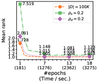
(a) Mean rank ($\blacktriangledown$) vs. #epochs 

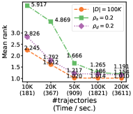
(b) Mean rank ($\blacktriangledown$) vs. #trajectories  

Figure 5: Impact of model training

Impact of the number of the training epochs. Fig. 4a shows the learning curve of TrajCL from 1 to 18 epochs of one run (when early termination is triggered and hence a time different from that in Table VII is reported). As expected, TrajCL produces lower mean ranks (i.e., better model accuracy) when it is trained for more epochs. By the 7th epoch (about 20 minutes), TrajCL has already achieved a satisfactory performance. This shows that TrajCL is easy to train and converge, which helps its scalability.

Impact of the number of training trajectories. As Fig. 4b shows, TrajCL benefits from more training trajectories. This is expected as more training trajectories offer more examples for the model to learn the different data patterns from. The performance gains diminish when using more than 50,000 original trajectories for training, while it takes a few more training trajectories when they are down-sampled or distorted, which is also intuitive. Using 50,000 trajectories, TrajCL only takes about 15 minutes to train, which is quite practical. We used 200,000 as the default training set size, since the baseline methods require at least this size [11, 12, 14, 13].

V-E Efficiency of $K$ Nearest Neighbor Queries

In real applications, we may index the trajectory database $D$ to support fast similarity searches. We test TrajCL under such a setting. To the best of our knowledge, this is the first reported results for $k$NN queries over trajectories using a non-trivial algorithm (i.e., non-full scans) based on learned embeddings.

Setup. We generate three trajectory databases $D$ with $|D|=0.1,1$ and $10$ million, by distorting ($\rho_{d}=0.2$) randomly selected trajectories from the Xi’an dataset which has the largest number of points per trajectory. The three datasets have 11.8 million, 118.0 million and 1.2 billion trajectory points, respectively. We use the same 1,000 trajectory query sets as before, and run $k$NN queries over the generated databases.

We run TrajCL to generate embeddings for the data trajectories and index them with Faiss [52] which is a widely used library for similarity queries over dense vectors based on a Voronoi diagram. Note that our aim here is not to come up with another trajectory index but to test the query efficiency of TrajCL embeddings with existing $k$NN algorithms.

We compare with Hausdorff, since the other learned methods will share the same query efficiency with TrajCL on Faiss, while Hausdorff is the fastest heuristic measure (cf. Table V-C). For Hausdorff, we build a segment-based index with $k$NN pruning strategies, following a recent work DFT [1].

Results. $k$NN query. Fig. 6 shows the total response times to run 1,000 $k$NN queries, which grow with the dataset size $|D|$ for both methods, as expected. TrajCL is about two orders of magnitude faster than Hausdorff, which attributes to both the fast embedding-based similarity computation and the efficient query procedure enabled by the embedding vectors. The Hausdorff index triggers an out-of-memory error when $|D|=10$M and hence no results were obtained for this case.

Figure 6: $k$NN query costs

TABLE IX: Index building costs

3	$|D|$	Time (sec)	RAM (GB)
Hausdorff	0.1M	20.7	2.8
	1M	256.3	30.8
	10M	-	OOM
TrajCL	0.1M	42.7	0.5
	1M	426.1	2.9
	10M	4,234.0	20.3
3

Index construction. Table IX further reports the index construction costs, which also grow with $|D|$. The TrajCL index (i.e., Faiss) takes about twice the time of the Hausdorff index (i.e., DFT) to build, where the extra times are spent on converting the trajectories to their embeddings. However, the TrajCL index takes much less memory than the Hausdorff index, e.g., 2.9 GB vs. 30.8 GB when $|D|=1$M. This is because DFT needs to store auxiliary data for query pruning, which causes the out-of-memory error when $|D|=10$M (1.2 billion segments, while DFT is a segment-based index).

TABLE X: HR@5, HR@20 and R5@20 ($\blacktriangle$) of self-supervised and supervised methods to approximate heuristic measures

3 Dataset	Category	Method	EDR			EDwP			Hausdorff			Fréchet			Average rank ($\blacktriangledown$)
			HR@5	HR@20	R5@20	HR@5	HR@20	R5@20	HR@5	HR@20	R5@20	HR@5	HR@20	R5@20
Porto	Pre-trained + fine-tuning	t2vec	0.125	0.164	0.286	0.399	0.518	0.751	0.405	0.549	0.770	0.504	0.651	0.883	5
		TrjSR	0.137	0.147	0.273	0.271	0.346	0.535	0.541	0.638	0.880	0.271	0.356	0.523	8
		E2DTC	0.122	0.157	0.272	0.390	0.514	0.742	0.391	0.537	0.753	0.498	0.648	0.879	6
		CSTRM	0.138	0.191	0.321	0.415	0.536	0.753	0.459	0.584	0.813	0.421	0.557	0.768	3
		TrajCL	0.169	0.220	0.373	0.506	0.615	0.845	0.570	0.670	0.909	0.554	0.674	0.897	2
		TrajCL∗	0.172	0.222	0.376	0.546	0.646	0.881	0.643	0.721	0.954	0.618	0.740	0.955	1
	Supervised	Traj2SimVec	0.119	0.163	0.285	0.172	0.253	0.390	0.339	0.429	0.543	0.529	0.664	0.894	9
		TrajGAT	0.090	0.102	0.184	0.201	0.274	0.469	0.686	0.740	0.969	0.362	0.403	0.704	7
		T3S	0.140	0.192	0.325	0.377	0.498	0.702	0.329	0.482	0.668	0.595	0.728	0.946	4
Chengdu	Pre-trained + fine-tuning	t2vec	0.144	0.250	0.332	0.285	0.364	0.539	0.347	0.510	0.681	0.479	0.607	0.823	6
		TrjSR	0.137	0.245	0.347	0.210	0.251	0.430	0.555	0.690	0.887	0.369	0.472	0.671	7
		E2DTC	0.136	0.241	0.317	0.269	0.348	0.518	0.319	0.484	0.647	0.461	0.585	0.802	8
		CSTRM	0.153	0.239	0.354	0.342	0.391	0.642	0.541	0.665	0.871	0.519	0.629	0.848	3
		TrajCL	0.171	0.258	0.382	0.366	0.405	0.665	0.594	0.715	0.918	0.602	0.697	0.918	2
		TrajCL∗	0.178	0.271	0.404	0.381	0.429	0.671	0.697	0.785	0.968	0.726	0.794	0.981	1
	Supervised	Traj2SimVec	0.140	0.239	0.356	0.181	0.313	0.487	0.183	0.257	0.409	0.240	0.325	0.594	9
		TrajGAT	0.091	0.188	0.261	0.257	0.373	0.612	0.695	0.771	0.970	0.435	0.496	0.853	5
		T3S	0.149	0.237	0.346	0.330	0.417	0.605	0.440	0.582	0.741	0.498	0.622	0.831	4
Xi’an	Pre-trained + fine-tuning	t2vec	0.162	0.244	0.361	0.272	0.317	0.494	0.354	0.514	0.683	0.445	0.565	0.774	6
		TrjSR	0.151	0.267	0.391	0.218	0.273	0.439	0.536	0.661	0.843	0.379	0.464	0.685	7
		E2DTC	0.152	0.232	0.344	0.244	0.291	0.455	0.317	0.472	0.628	0.400	0.529	0.724	8
		CSTRM	0.161	0.244	0.360	0.336	0.364	0.522	0.522	0.656	0.848	0.497	0.605	0.816	5
		TrajCL	0.178	0.269	0.399	0.360	0.414	0.672	0.580	0.705	0.901	0.592	0.687	0.908	2
		TrajCL∗	0.181	0.277	0.413	0.362	0.424	0.677	0.695	0.779	0.964	0.690	0.769	0.966	1
	Supervised	Traj2SimVec	0.143	0.255	0.388	0.163	0.287	0.491	0.130	0.217	0.372	0.156	0.254	0.487	9
		TrajGAT	0.131	0.269	0.387	0.312	0.440	0.696	0.739	0.787	0.976	0.476	0.537	0.884	3
		T3S	0.175	0.272	0.408	0.328	0.439	0.617	0.423	0.601	0.782	0.539	0.651	0.848	4
Germany	Pre-trained + fine-tuning	t2vec	0.050	0.373	0.382	0.211	0.260	0.391	0.202	0.240	0.357	0.204	0.257	0.374	7
		TrjSR	0.029	0.311	0.346	0.234	0.288	0.451	0.445	0.606	0.780	0.400	0.573	0.745	6
		E2DTC	0.047	0.338	0.378	0.198	0.244	0.369	0.196	0.235	0.346	0.200	0.254	0.369	8
		CSTRM	-	-	-	-	-	-	-	-	-	-	-	-	9
		TrajCL	0.114	0.406	0.433	0.444	0.603	0.740	0.506	0.612	0.810	0.531	0.663	0.857	2
		TrajCL∗	0.127	0.427	0.461	0.486	0.679	0.908	0.619	0.736	0.919	0.620	0.755	0.922	1
	Supervised	Traj2SimVec	0.073	0.386	0.437	0.309	0.433	0.584	0.428	0.634	0.812	0.456	0.640	0.883	4
		TrajGAT	0.081	0.402	0.442	0.452	0.648	0.833	0.563	0.658	0.889	0.411	0.537	0.722	3
		T3S	0.044	0.358	0.365	0.443	0.590	0.733	0.423	0.515	0.657	0.415	0.564	0.756	5
3

V-F Approximating Heuristic Measures

We investigate the generalizability of TrajCL by fine-tuning a pre-trained TrajCL to learn and approximate a heuristic similarity measure with very few labelled data. To the best of our knowledge, this is the first study to investigate the effectiveness of a learning-based trajectory similarity measure to approximate a heuristic measure. The fine-tuned TrajCL can be used as a fast estimator for fast online computation of an expensive heuristic similarity measure (e.g., EDwP).

Setup. We take the trained encoder of TrajCL (and other self-supervised methods) on each dataset from Section V-B and connect it with a two-layer MLP where the size of each layer is the same as $d$. We fine-tune the last layer of the encoder and train the MLP to predict a given heuristic similarity value, optimizing the MSE loss. Besides the above self-supervised methods and the state-of-the-art supervised methods mentioned in Section V-A, we also add an variant to show the optimal performance of TrajCL where all layers of the encoder are fine-tuned, named TrajCL^∗.

Following the supervised methods [19, 21, 20], we report the hit ratio results HR@$k$ ($k=5,20$), i.e., the ratio of the ground-truth top-$k$ trajectories in the predicted top-$k$ results, and R5@20, which denotes the recall of returning the ground-truth top-5 trajectories in the predicted top-20 results. We also report the average rank of each method over the 4 measures and 3 metrics on each dataset.

Results. Table X summarizes the results. Overall, TrajCL^∗ achieves the best similarity prediction accuracy (i.e., average rank is 1), while TrajCL ranks the second.

Comparing with the self-supervised baselines t2vec, TrjSR and E2DTC, TrajCL^∗ and TrajCL produce higher HR@5, HR@20 and R5@20 scores consistently. Based on HR@5, TrajCL gains improvements by up to 128.0%, 89.7%, 41.5% and 32.7% to approximate EDR, EDwP, Hausdorff and Fréchet, respectively. TrajCL^∗ further improves over TrajCL by up to 11.4%, 9.4%, 22.3% and 20.6% on approximating the four heuristic measures, respectively. Similar trends can be observed on HR@20 and R5@20. The high R5@20 scores of TrajCL^∗ and TrajCL for Hausdorff and Fréchet, i.e., almost all over 0.9 on all four datasets, show that our models can approximate the two measures very well, since they are directly based on the spatial distances between point pairs.

Compared with the supervised methods Traj2SimVec, TrajGAT and T3S, TrajCL^∗ is better in 80% of the cases, i.e., 38 out of the 48 cases tested. When TrajCL^∗ performs better, its performance gain is 14.6% on average. On the contrary, when a supervised baseline performs better, the average performance gap is just 2.8%. Such cases are mostly observed on approximating Hausdorff, and the strong performance of TrajGAT in these cases is consistent with its own study [21].

These confirm that the pre-trained TrajCL models can be easily adapted to approximate a given heuristic similarity measure. Such generalizability attributes to the trajectory augmentation methods and the TrajCL encoder.

V-G Ablation Study

We study the impact of model components and augmentation methods in TrajCL in this section.

Impact of the model components. We compare TrajCL with two model variants: (1) TrajCL-MSM replaces DualMSM with the vanilla MSM used in Transformer. This variant also ignores the spatial features S. It can be regarded as applying a vanilla Transformer encoder in our proposed trajectory contrastive learning framework. (2) TrajCL-concat also uses the vanilla MSM, but it concatenates the spatial features with the structural features, i.e., $\mathbf{T}\|\mathbf{S}$, as the input.

We repeat the two sets of experiments of Sections V-B and V-F, i.e., running our models on their own (denoted as “no fine-tuning”) and fine-tuning them to approximate a heuristic similarity measure (denoted as “with fine-tuning”). When running our models on their own, we follow the settings in Section V-D. When fine-tuning our models to approximate a heuristic measure, we report HR@5. We only present the results on Porto for conciseness, since similar comparative patterns are observed on the other datasets.

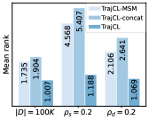
(a) No fine-tuning ($\blacktriangledown$) 

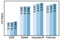
(b) With fine-tuning ($\blacktriangle$, HR@5)  

Figure 7: Ablation study results

Results. Fig. 6a shows the results on TrajCL variants without fine-tuning. TrajCL performs better than the two variants by reducing the mean rank of $T^{q}_{b}$ by at least 72.29% and 89.08%, respectively. TrajCL-concat performs the worst, even though it uses the spatial features while TrajCL-MSM does not, as a direct concatenation can confuse the feature space of the model. The result highlights the importance of DualMSM that adaptively fuses both type of input features.

Fig. 6b shows the results with fine-tuning. TrajCL still outperforms the two variants overall, except when approximating EDwP where all variants have similar results. This confirms that our DualMSM module has a strong generalization capability to capture the similarity between trajectories such that the fine-tuned TrajCL can make more accurate predictions.

Impact of the augmentation methods. Next, we study how augmentation methods affect model performance by varying the augmentation methods to generate $\widetilde{T}$ and $\widetilde{T}^{\prime}$. We use the same experimental setup as the last experiment. We only report the mean ranks on $|D|$=100K without fine-tuning and report the fine-tuning results of approximating EDwP (the most accurate but slowest heuristic measure), due to similar comparative patterns observed on other metrics.

Results. As Fig. 8 shows, overall, augmentation helps TrajCL learn more robust embeddings. TrajCL without data augmentation (i.e., Raw&Raw, using $T$ as $\widetilde{T}$ and $\widetilde{T}^{\prime}$) has the lowest (i.e., worst) HR@5 value in Fig. 7b and the second-largest (i.e., worst but second) mean rank values in Fig. 7a. Such results confirm the importance of the proposed augmentation methods. Further, using the same augmentation methods for both $\widetilde{T}$ and $\widetilde{T}^{\prime}$ may be sub-optimal, as this limits the learning space. Overall, point masking and trajectory truncating (i.e., Mask&Trun.) produce the best similarity learning results, and thus have been used by default.

Point masking helps learn the correlation between non-adjacent points and hence makes TrajCL adaptive to trajectories with different sampling rates. Meanwhile, trajectory truncating helps learn the similarity between partial trajectories and the full ones. In comparison, point shifting aims to guide TrajCL to learn to overcome noises, while the grid cells used in TrajCL can already achieve a similar purpose. Also, trajectory simplification may remove too many points and hence miss key movement patterns to reflect trajectory similarity.

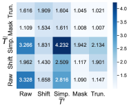
(a) Mean rank ($\blacktriangledown$, $|D|$=100K) 

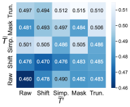
(b) HR@5 ($\blacktriangle$, with fine-tuning) 

Figure 8: Impact of the augmentation methods (Lighter color is better. Raw, Shift, Mask, Trun. and Simp. denote no augmentation, point shifting, point masking, trajectory truncating and trajectory simplification, respectively.)

Impact of parameters in augmentation methods. We focus on $\rho_{d}$ and $\rho_{b}$ for the two default augmentation methods point masking and trajectory truncating, respectively.

Results. We vary $\rho_{d}$ and $\rho_{b}$ from 0.1 to 0.9, respectively. As Fig. 9 shows, overall, TrajCL is not heavily impacted by the two parameters unless for extreme values 0.1 and 0.9, i.e., when the augmented trajectories are too or little different from the original ones. When $\rho_{d}\in\{0.3,0.5\}$ and $\rho_{b}\in\{0.5,0.7\}$, TrajCL performs the best. We use 0.3 and 0.7 by default for $\rho_{d}$ and $\rho_{b}$, respectively, where the lowest (i.e., best) mean rank is reached while HR@5 is also close to the best.

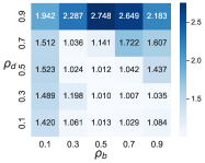
(a) Mean rank ($\blacktriangledown$, $|D|$=100K) 

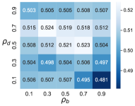
(b) HR@5 ($\blacktriangle$, with fine-tuning) 

Figure 9: Impact of parameters of the augmentation methods

V-H Parameter Study

We further study the impact of model parameters using the same experimental setup as Section V-G.

Impact of the embedding dimensionality $d$. We vary $d$ from 64 to 1,024. As Fig. 10 shows, overall, TrajCL performs better when $d\leqslant 256$ without fine-tuning. This is because a large embedding dimensionality results in overfitting which impacts the similarity prediction results. When TrajCL is fine-tuned, on the other hand, a larger $d$ allows it to better approximate heuristic measures. We note that a large $d$ also means larger fine-tuning and inference times. Thus, we have used 256 by default to balance model accuracy and efficiency.

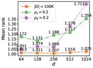
(a) No fine-tuning ($\blacktriangledown$) 

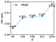
(b) With fine-tuning ($\blacktriangle$) 

Figure 10: Impact of the embedding dimensionality

Impact of the number of the encoder layers $\#layers$. Fig. 11 shows the results for $\#layers\in[1,5]$. As $\#layers$ increases, the model performance first improves and then drops when $\#layers$ exceeds 4. This is because adding more layers yields better feature generalization capability at first, since more layers help learn more complicated non-linear functions. When there are too many layers, however, it causes the model to overfit the training data. Given that a model with more layers takes substantially more time to train and run, we have only used a 2-layer encoder by default.

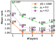
(a) No fine-tuning ($\blacktriangledown$) 

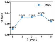
(b) With fine-tuning ($\blacktriangle$)  

Figure 11: Impact of the number of the encoder layers

Impact of the size of the negative sample queue $|Q_{neg}|$. Lastly, we vary $|Q_{neg}|$ from 512 to 8,192. As Fig. 12 shows, when $|Q_{neg}|$ increases, TrajCL  performs better in general, i.e., the mean ranks decrease and HR@5 increases. This is because more negative samples help reduce the bias caused by a small sample set, leading to more uniformly distributed embeddings in the latent space. As before, a large $|Q_{neg}|$ also leads to a larger training cost. We thus have used 2,048 by default.

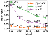
(a) No fine-tuning ($\blacktriangledown$) 

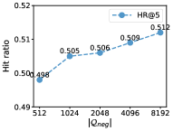
(b) With fine-tuning ($\blacktriangle$) 

Figure 12: Impact of the size of the negative sample queue

VI Conclusion

We proposed TrajCL, a self-supervised trajectory similarity learning model that comes with a set of trajectory augmentation methods and a dual-feature multi-head self-attention-based trajectory backbone encoder. TrajCL can learn the inherent similarity between trajectories and approximate predefined heuristic trajectory similarity measures. This makes TrajCL a highly applicable trajectory similarity computation method. Experiments on four real trajectory datasets show that, compared with the state-of-the-art methods, TrajCL achieves significant improvements in the accuracy for measuring trajectory similarity and approximating a heuristic measure.

Acknowledgment

This work is partially supported by Australian Research Council (ARC) Discovery Project DP230101534. We thank Prof. Gao Cong for his comments which helped improve the paper.

References

- [1] D. Xie, F. Li, and J. M. Phillips, “Distributed Trajectory Similarity Search,” PVLDB, vol. 10, no. 11, pp. 1478–1489, 2017.
- [2] H. Yuan and G. Li, “Distributed In-Memory Trajectory Similarity Search and Join on Road Network,” in ICDE, 2019, pp. 1262–1273.
- [3] S. Shang, L. Chen, Z. Wei, C. S. Jensen, K. Zheng, and P. Kalnis, “Trajectory Similarity Join in Spatial Networks,” PVLDB, vol. 10, no. 11, pp. 1178–1189, 2017.
- [4] S. Wang, Z. Bao, J. S. Culpepper, Z. Xie, Q. Liu, and X. Qin, “Torch: A Search Engine for Trajectory Data,” in SIGIR, 2018, pp. 535–544.
- [5] Y. Chang, J. Qi, E. Tanin, X. Ma, and H. Samet, “Sub-Trajectory Similarity Join with Obfuscation,” in SSDBM, 2021, pp. 181–192.
- [6] Z. Shang, G. Li, and Z. Bao, “DITA: Distributed In-Memory Trajectory Analytics,” in SIGMOD, 2018, pp. 725–740.
- [7] L. Chen, M. T. Özsu, and V. Oria, “Robust and Fast Similarity Search for Moving Object Trajectories,” in SIGMOD, 2005, pp. 491–502.
- [8] S. Ranu, P. Deepak, A. D. Telang, P. Deshpande, and S. Raghavan, “Indexing and Matching Trajectories under Inconsistent Sampling Rates,” in ICDE, 2015, pp. 999–1010.
- [9] H. Alt, “The Computational Geometry of Comparing Shapes,” in Efficient Algorithms, 2009, pp. 235–248.
- [10] H. Alt and M. Godau, “Computing the Fréchet Distance between Two Polygonal Curves,” International Journal of Computational Geometry & Applications, vol. 5, no. 01n02, pp. 75–91, 1995.
- [11] X. Li, K. Zhao, G. Cong, C. S. Jensen, and W. Wei, “Deep Representation Learning for Trajectory Similarity Computation,” in ICDE, 2018, pp. 617–628.
- [12] H. Cao, H. Tang, Y. Wu, F. Wang, and Y. Xu, “On Accurate Computation of Trajectory Similarity via Single Image Super-Resolution,” in IJCNN, 2021, pp. 1–9.
- [13] X. Liu, X. Tan, Y. Guo, Y. Chen, and Z. Zhang, “CSTRM: Contrastive Self-Supervised Trajectory Representation Model for Trajectory Similarity Computation,” Computer Communications, vol. 185, pp. 159–167, 2022.
- [14] Z. Fang, Y. Du, L. Chen, Y. Hu, Y. Gao, and G. Chen, “E2DTC: An End to End Deep Trajectory Clustering Framework via Self-training,” in ICDE, 2021, pp. 696–707.
- [15] “Porto Taxi Trajectory Dataset,” https://www.kaggle.com/c/pkdd-15-predict-taxi-service-trajectory-i, 2022.
- [16] K. He, H. Fan, Y. Wu, S. Xie, and R. Girshick, “Momentum Contrast for Unsupervised Visual Representation Learning,” in CVPR, 2020, pp. 9729–9738.
- [17] T. Chen, S. Kornblith, M. Norouzi, and G. Hinton, “A Simple Framework for Contrastive Learning of Visual Representations,” in ICML, 2020, pp. 1597–1607.
- [18] D. Yao, G. Cong, C. Zhang, and J. Bi, “Computing Trajectory Similarity in Linear Time: A Generic Seed-guided Neural Netric learning approach,” in ICDE, 2019, pp. 1358–1369.
- [19] H. Zhang, X. Zhang, Q. Jiang, B. Zheng, Z. Sun, W. Sun, and C. Wang, “Trajectory Similarity Learning with Auxiliary Supervision and Optimal Matching,” in IJCAI, 2020, pp. 11–17.
- [20] P. Yang, H. Wang, Y. Zhang, L. Qin, W. Zhang, and X. Lin, “T3S: Effective Representation Learning for Trajectory Similarity Computation,” in ICDE, 2021, pp. 2183–2188.
- [21] D. Yao, H. Hu, L. Du, G. Cong, S. Han, and J. Bi, “TrajGAT: A Graph-based Long-term Dependency Modeling Approach for Trajectory Similarity Computation,” in KDD, 2022, pp. 2275–2285.
- [22] Y. Yanagisawa, J.-i. Akahani, and T. Satoh, “Shape-Based Similarity Query for Trajectory of Mobile Objects,” in MDM, 2003, pp. 63–77.
- [23] M. Vlachos, G. Kollios, and D. Gunopulos, “Discovering Similar Multidimensional Trajectories,” in ICDE, 2002, pp. 673–684.
- [24] L. Chen and R. Ng, “On the Marriage of LP-Norms and Edit Distance,” in VLDB, 2004, pp. 792–803.
- [25] P. Han, J. Wang, D. Yao, S. Shang, and X. Zhang, “A Graph-based Approach for Trajectory Similarity Computation in Spatial Networks,” in KDD, 2021, pp. 556–564.
- [26] Z. Fang, Y. Du, X. Zhu, L. Chen, Y. Gao, and C. S. Jensen, “ST2Vec: Spatio-Temporal Trajectory Similarity Learning in Road Networks,” arXiv preprint arXiv:2112.09339, 2021.
- [27] Y. Chang, E. Tanin, X. Cao, and J. Qi, “Spatial Structure-Aware Road Network Embedding via Graph Contrastive Learning,” in EDBT, 2023.
- [28] S. Hochreiter and J. Schmidhuber, “Long Short-Term Memory,” Neural Computation, vol. 9, no. 8, pp. 1735–1780, 1997.
- [29] A. Vaswani, N. Shazeer, N. Parmar, J. Uszkoreit, L. Jones, A. N. Gomez, Ł. Kaiser, and I. Polosukhin, “Attention Is All You Need,” in NeurIPS, 2017, p. 6000–6010.
- [30] X. Chen, H. Fan, R. Girshick, and K. He, “Improved Baselines with Momentum Contrastive Learning,” arXiv preprint arXiv:2003.04297, 2020.
- [31] M. Caron, I. Misra, J. Mairal, P. Goyal, P. Bojanowski, and A. Joulin, “Unsupervised Learning of Visual Features by Contrasting Cluster Assignments,” in NeurIPS, 2020, pp. 9912–9924.
- [32] H. Fang, S. Wang, M. Zhou, J. Ding, and P. Xie, “CERT: Contrastive Self-Supervised Learning for Language Understanding,” arXiv preprint arXiv:2005.12766, 2020.
- [33] T. Gao, X. Yao, and D. Chen, “SimCSE: Simple Contrastive Learning of Sentence Embeddings,” in EMNLP, 2021, pp. 6894–6910.
- [34] J. Giorgi, O. Nitski, B. Wang, and G. Bader, “DeCLUTR: Deep Contrastive Learning for Unsupervised Textual Representations,” in ACL, 2021, pp. 879–895.
- [35] P. Veličković, W. Fedus, W. L. Hamilton, P. Liò, Y. Bengio, and R. D. Hjelm, “Deep Graph Infomax,” in ICLR, 2018.
- [36] K. Hassani and A. H. Khasahmadi, “Contrastive Multi-View Representation Learning on Graphs,” in ICML, 2020, pp. 4116–4126.
- [37] J. Qiu, Q. Chen, Y. Dong, J. Zhang, H. Yang, M. Ding, K. Wang, and J. Tang, “GCC: Graph Contrastive Coding for Craph Neural Network Pre-Training,” in KDD, 2020, pp. 1150–1160.
- [38] Y. Zhu, Y. Xu, F. Yu, Q. Liu, S. Wu, and L. Wang, “Graph Contrastive Learning with Adaptive Augmentation,” in WWW, 2021, pp. 2069–2080.
- [39] X. Liu, Y. Liang, C. Huang, Y. Zheng, B. Hooi, and R. Zimmermann, “When Do Contrastive Learning Signals Help Spatio-Temporal Graph Forecasting?” in SIGSPATIAL, 2022.
- [40] J. Devlin, M.-W. Chang, K. Lee, and K. Toutanova, “BERT: Pre-training of Deep Bidirectional Transformers for Language Understanding,” in NAACL, 2019, pp. 4171–4186.
- [41] A. Dosovitskiy, L. Beyer, A. Kolesnikov, D. Weissenborn, X. Zhai, T. Unterthiner, M. Dehghani, M. Minderer, G. Heigold, S. Gelly et al., “An Image is Worth 16x16 Words: Transformers for Image Recognition at Scale,” in ICLR, 2020.
- [42] Z. Liu, Y. Lin, Y. Cao, H. Hu, Y. Wei, Z. Zhang, S. Lin, and B. Guo, “Swin Transformer: Hierarchical Vision Transformer using Shifted Windows,” in ICCV, 2021, pp. 10 012–10 022.
- [43] A. v. d. Oord, Y. Li, and O. Vinyals, “Representation Learning with Contrastive Predictive Coding,” arXiv preprint arXiv:1807.03748, 2018.
- [44] F. Wang and H. Liu, “Understanding the Behaviour of Contrastive Loss,” in CVPR, 2021, pp. 2495–2504.
- [45] D. H. Douglas and T. K. Peucker, “Algorithms for the Reduction of the Number of Points Required to Represent a Digitized Line or its Caricature,” Cartographica: The International Journal for Geographic Information and Geovisualization, vol. 10, no. 2, pp. 112–122, 1973.
- [46] A. Grover and J. Leskovec, “node2vec: Scalable Feature Learning for Networks,” in KDD, 2016, pp. 855–864.
- [47] K. He, X. Zhang, S. Ren, and J. Sun, “Deep Residual Learning for Image Recognition,” in CVPR, 2016, pp. 770–778.
- [48] N. Srivastava, G. Hinton, A. Krizhevsky, I. Sutskever, and R. Salakhutdinov, “Dropout: A Simple Way to Prevent Neural Networks from Overfitting,” Journal of Machine Learning Research, vol. 15, no. 1, pp. 1929–1958, 2014.
- [49] J. L. Ba, J. R. Kiros, and G. E. Hinton, “Layer Normalization,” arXiv preprint arXiv:1607.06450, 2016.
- [50] “DiDi GAIA Open Dataset,” https://outreach.didichuxing.com/en/, 2022.
- [51] “OpenStreetMap Public Route Dataset,” https://wiki.openstreetmap.org/wiki/Planet.gpx, 2013.
- [52] J. Johnson, M. Douze, and H. Jégou, “Billion-Scale Similarity Search with GPUs,” IEEE Transactions on Big Data, vol. 7, no. 3, pp. 535–547, 2019.