Understanding the Failure of Batch Normalization for Transformers in NLP

Abstract

Batch Normalization (BN) is a core and prevalent technique in accelerating the training of deep neural networks and improving the generalization on Computer Vision (CV) tasks. However, it fails to defend its position in Natural Language Processing (NLP), which is dominated by Layer Normalization (LN). In this paper, we are trying to answer why BN usually performs worse than LN in NLP tasks with Transformer models. We find that the inconsistency between training and inference of BN is the leading cause that results in the failure of BN in NLP. We define Training Inference Discrepancy (TID) to quantitatively measure this inconsistency and reveal that TID can indicate BN’s performance, supported by extensive experiments, including image classification, neural machine translation, language modeling, sequence labeling, and text classification tasks. We find that BN can obtain much better test performance than LN when TID keeps small through training. To suppress the explosion of TID, we propose Regularized BN (RBN) that adds a simple regularization term to narrow the gap between batch statistics and population statistics of BN. RBN improves the performance of BN consistently and outperforms or is on par with LN on 17 out of 20 settings, involving ten datasets and two common variants of Transformer.

1 Introduction

Deep learning [21] has revolutionized Computer Vision (CV) [20] and Natural Language Processing (NLP) [41]. Normalization layers are key components to stabilize and accelerate the training in Deep Neural Networks (DNNs). In CV, Batch Normalization (BN) [17] is the default normalization technique and reveals superior performance over other normalization techniques in image recognition tasks by enforcing the input of a neuron to have zero mean and unit variance within a mini-batch data. Furthermore, a growing number of theoretical works analyze the excellent properties of BN in benefiting optimization [17, 36, 4, 13, 8, 9]. While BN almost dominates in CV with empirical success and theoretical properties, Layer Normalization (LN) is the leading normalization technique in NLP, especially for Transformer models that achieve the state-of-the-art performance on extensive tasks, including machine translation [41], natural language understanding [10], text generation [34], few shot learning [5], to name a few. As a direct substitute of LN, BN performs poorly in Transformer for neural machine translation [38]. It remains elusive to explain the failure of BN in NLP community. In this work, we are trying to take a step forward. Our contributions are summarized as follows:

• We find that the inconsistency between training and inference leads to the failure of BN in NLP, supported by our extensive experiments, including image classification, neural machine translation, language modeling, sequence labeling, and text classification tasks.

• We define Training Inference Discrepancy (TID) to quantitatively measure this inconsistency and show that TID can serve as an indicator of BN’s performance. In particular, BN reaches much better test performance than LN when TID keeps small through training, e.g., in image recognition and language modeling tasks.

• We propose Regularized BN (RBN) that adds a regularization term in BN to penalize and reduce the TID when the TID of BN is large. We reveal the optimization advantages of RBN over LN by exploring the layer-wise training dynamics of Transformer.

• We empirically show that RBN can exceed or match the performance of LN, sometimes with a large margin, on 17 out of 20 settings, involving ten datasets and two common variants of Transformer. Besides, RBN introduces no extra computation at inference compared to LN.

2 Related Work

Analyses of BN’s Success

As BN becomes an indispensable component in deep neural networks deployed in CV tasks, a bunch of works explore the theoretical reasons behind its success. From the view of optimization, the original BN paper [17] argues that BN can reduce internal covariate shift and thus stabilize the training, while Santurkar et al. [36] debate that BN could smooth the loss landscape and thus enable training of neural network with larger learning rate [4]. Daneshmand et al. [8, 9] prove that a stack of randomized linear layers and BN layers will endow the intermediate features of neural network with sufficient numerical rank as depth increases, which is beneficial for optimization and learning discriminative hierarchical features. Huang et al. [13] show that BN could improve the layer-wise conditioning of the neural network optimization by exploring the spectrum of Hessian matrix with block diagonal approximation [28]. From the view of generalization, Ioffe and Szegedy [17], Luo et al. [25], Li et al. [22], Wu and Johnson [43] argue that BN serves as regularizer which reduces over-fitting when its stochasticity is small and may have detrimental effect when it is large [43]. Huang et al. [12] further propose Stochastic Normalization Disturbance (SND) to measure such stochasticity and shows that large SND will hinder the training of neural networks.

Training Inference Inconsistency of BN

Normalizing along the batch dimension usually introduces training inference inconsistency since mini-batch data is neither necessary nor desirable during inference. BN uses population statistics, estimated by running average over mini-batch statistics, for inference. The training inference inconsistency usually harms the performance of BN for small-batch-size training since the estimation of population statistics could be inaccurate [42]. One way to reduce the inconsistency between training and inference is to exploit the estimated population statistics for normalization during training [16, 6, 47, 50, 49]. These works may outperform BN when the batch size is small, where inaccurate estimation may be the main issue [17, 18], but they usually work inferior to BN under moderate batch-size training [24]. Another way to reduce the inconsistency is estimating corrected normalization statistics during inference only, either for domain adaptation [23], corruption robustness [37, 31, 2], or small-batch-size training  [39, 40]. We note that a recent work [14] investigates the estimation shift problem of BN. Unlike this work that addresses the accumulated estimation shift due to the stack of BNs for CNNs in CV tasks, our work pays more attention to how the training inference inconsistency of BN correlates with its performances for Transformers in NLP tasks. Besides, the estimation shift of BN defined in [14], which addresses the differences between the estimated population statistics and the expected statistics, differs from our TID of BN that addresses the differences between the mini-batch statistics and populations statistics.

Exploring the Failure of BN in Transformer

Similar to our work, Power Normalization (PN) [38] also investigates the reason behind the failure of BN in Transformers. Our work significantly differs from PN [38] in the following facets. PN attributes the failure of BN to the unstable training of BN incurred by fluctuated forward and backward batch statistics with outlier values, while we observe that the training of BN is as good as LN and the inconsistency between training and inference of BN matters more. Based on our observation, we propose a regularization term to reduce the TID of BN. Compared with PN, which incorporates a layer-scale layer (root mean square layer normalization [51] without affine transformation [45]), our method introduces no extra computation at inference. Besides, we use a more reasonable index to measure inconsistency which is invariant to the scale of data. Furthermore, we show that our RBN can improve the layer-wise training dynamics of LN, which reveals the optimization advantages of RBN.

3 Analyses of Training Inference Inconsistency in $\text{Transformer}_{BN}$

3.1 Preliminary

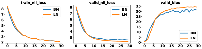
Figure 1: Train loss, validation loss/BLEU of Transformer trained on IWSLT14 with BN and LN. The training of $\text{Transformer}_{BN}$ is better than $\text{Transformer}_{LN}$ while the validation loss/BLEU of $\text{Transformer}_{BN}$ underperforms that of $\text{Transformer}_{LN}$ after 8 epoch. At the end of the training, $\text{Transformer}_{BN}$ falls behind $\text{Transformer}_{LN}$ with large BLEU scores. Lower loss and higher BLEU scores indicate better performance. Based on the inconsistency of training and validation performance of BN, we hypothesize that the training inference discrepancy of BN causes its performance degradation.

Batch Normalization (BN) [17] is typically used to stabilize and accelerate DNN’s training. Let $\mathbf{x}\in\mathbb{R}^{d}$ denote the $d$-dimensional input to a neural network layer. During training, BN standardizes each neuron/channel within $m$ mini-batch data by

$$\hat{\mathbf{x}}_{j}=BN_{train}(\mathbf{x}_{j})=\frac{\mathbf{x}_{j}-\mu_{B,j}}{\sqrt{\sigma^{2}_{B,j}}},~{}~{}j=1,2,...,d,$$ (1)

where $\mu_{B,j}=\frac{1}{m}\sum_{i=1}^{m}\mathbf{x}_{j}^{(i)}$ and $\sigma^{2}_{B,j}=\frac{1}{m}\sum_{i=1}^{m}(\mathbf{x}_{j}^{(i)}-\mu_{B,j})^{2}$ are the mini-batch mean and variance for each neuron, respectively. Note that an extra small number $\epsilon$ is usually added to the variance in practice to prevent numerical instability. During inference, the population mean $\mu$ and variance $\sigma^{2}$ of the layer input are required for BN to make a deterministic prediction [17] as:

$$\hat{\mathbf{x}}_{j}=BN_{inf}(\mathbf{x}_{j})=\frac{\mathbf{x}_{j}-\mu_{j}}{\sqrt{\sigma^{2}_{j}}},~{}~{}j=1,2,...,d.$$ (2)

These population statistics $\{\mu,\sigma^{2}\}$ are usually calculated as the running average of mini-batch statistics over different training iteration $t$ with an update factor $\alpha$ as follows:

$$\begin{cases}\quad\mu^{(t)}=(1-\alpha)\mu^{(t-1)}+\alpha\mu^{(t)}_{B},\\ \quad(\sigma^{2})^{(t)}=(1-\alpha)(\sigma^{2})^{(t-1)}+\alpha(\sigma^{2}_{B})^{(t)}.\end{cases}$$ (3)

The discrepancy of BN for normalization during training (using Eqn. 1) and inference (using Eqn. 2) can produce stochasticity, since the population statistics of BN are estimated from the mini-batch statistics that depend on the sampled mini-batch inputs. This discrepancy is believed to benefit the generalization [17, 12] if the stochasticity is well controlled. However, this discrepancy usually harms the performance of small-batch-size training [42] since the estimation of population statistics can be inaccurate. To address this problem, a bunch of batch-free normalizations are proposed that use consistent operations during training and inference, e.g., Layer Normalization (LN) [1].

Basic Observations

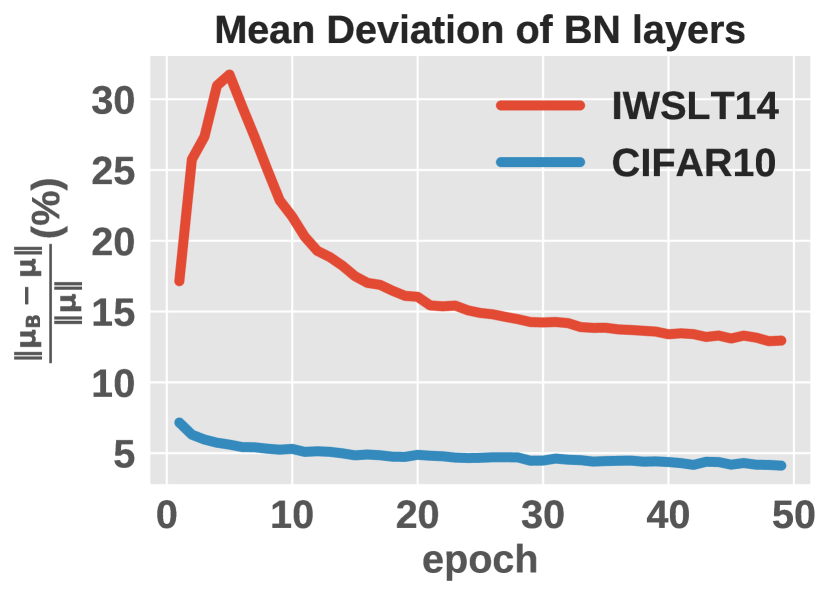
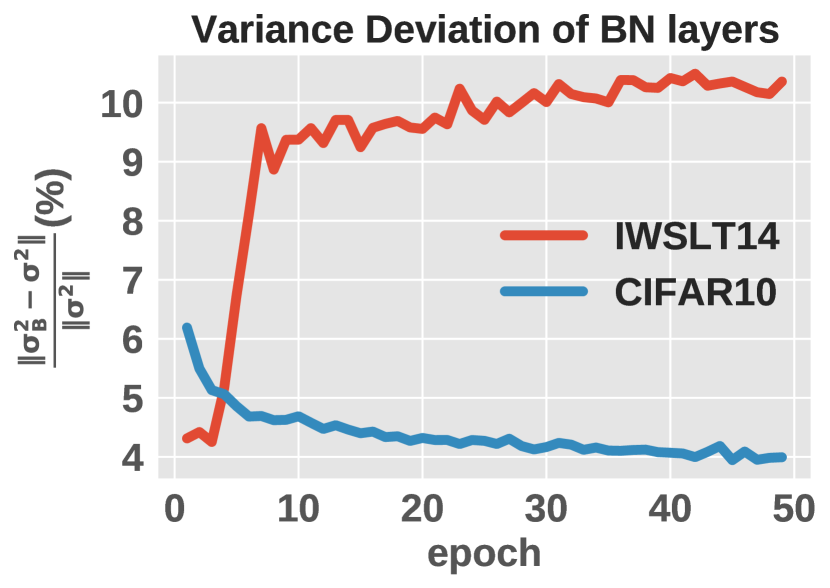
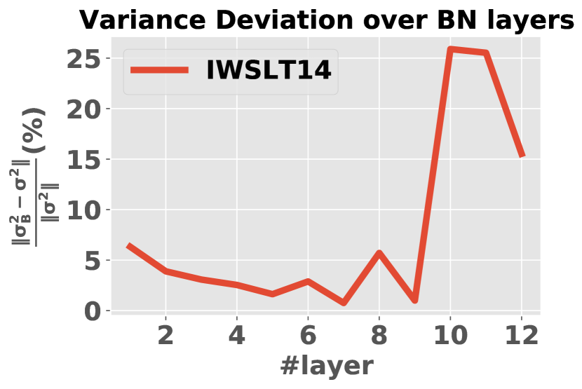
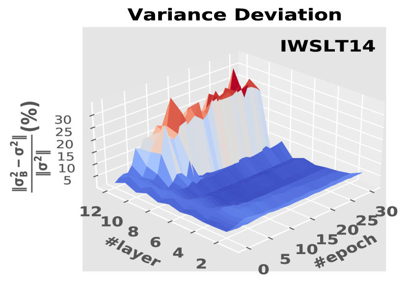
Figure 2: Top: The average deviation of batch mean $\mu_{B}$ (left figure) and batch variance $\sigma_{B}^{2}$ (right figure) to population mean $\mu$ and population variance $\sigma^{2}$ of all BN layers through training in ResNet18 and $\text{Transformer}_{BN}$. There are 21 BN layers in ResNet18 and 12 BN layers in the encoder of $\text{Transformer}_{BN}$. At the end of training, ResNet18 has mean/variance deviation of around $4\%$/$4\%$ and those in $\text{Transformer}_{BN}$ are around $11\%$/$13\%$. Large deviation of statistics hurts the performance of $\text{Transformer}_{BN}$. Bottom: Variance deviation of BN layers with different depths (left) at the end of training and variance deviation over depth and training progress (right).

To analyze the failure of BN in NLP tasks, we first plot the training loss and validation loss/BLEU [33] of BN and LN on IWSLT14 (De-En) dataset with the original Transformer model (see Figure 1). We observe that the training of $\text{Transformer}_{BN}$ is faster than $\text{Transformer}_{LN}$. The training nll_loss of BN is even smaller than that of LN, especially at the beginning. However, validation loss/BLEU of BN is worse than that of LN after around the seventh epoch. This phenomenon can not be attributed to over-fitting since BN introduces more stochasticity than LN in the training phase. The inconsistency between training and inference of BN may play a role.

Since BN in ResNet18 also involves training inference inconsistency, we guess the degree of such inconsistency has a difference between ResNet18 and $\text{Transformer}_{BN}$. Therefore, we plot the deviation of batch statistics to population statistics of BN in ResNet18 and $\text{Transformer}_{BN}$ in Figure 2 (top) to make a comparison. ResNet18 is trained on CIFAR-10 [19] and accuracy will drop 2 percent if we replace BN with LN. We find that at the end of the training, $\text{Transformer}_{BN}$ has a much bigger mean and variance deviation than ResNet18. Besides, the last several BN layers that are close to the output in $\text{Transformer}_{BN}$ have large variance deviation (Figure 2 (bottom)), which negatively impact the model output. Furthermore, the performance degradation of $\text{Transformer}_{BN}$ coincides with the increase of variance deviation by comparing Figure 1 (right) and Figure 2 (bottom right). Based on these observations, we hypothesize that the inconsistency between training and inference of BN causes BN’s performance degradation in neural machine translation. We first mathematically define the training inference discrepancy of BN in the next subsection.

3.2 Training Inference Discrepancy

By observing Eqns. 1 and 2, the normalized output during training can be calculated as:

$$\frac{\mathbf{x}_{j}-\mu_{B,j}}{\sigma_{B,j}}=\left(\frac{\mathbf{x}_{j}-\mu_{j}}{\sigma_{j}}+\frac{\mu_{j}-\mu_{B,j}}{\sigma_{j}}\right)\frac{\sigma_{j}}{\sigma_{B,j}},~{}~{}j=1,2,...,d,$$ (4)

where $\sigma_{B,j}>0$ and $\sigma_{j}>0$ are the standard deviation for the $j$-th dimension. We can see $\frac{\mu_{j}-\mu_{B,j}}{\sigma_{j}}$ and $\frac{\sigma_{j}}{\sigma_{B,j}}$ can be viewed as random variables. Their magnitude can characterize the diversity of mini-batch examples during training and indicate how hard the estimation of population statistics is. We thus define the training inference discrepancy to quantitatively measure the inconsistency as follows.

Definition 1 (Training Inference Discrepancy (TID)).

Let $p_{B}$ be the distribution of batch data. Given a mini-batch data $X$ sampled from $p_{B}$, we define the TID of its mean and variance (with respect to model parameter $\theta$) as:

Mean TID $$=\mathbb{E}_{X\sim p_{B}}\frac{\|\mu_{B}-\mu\|_{2}}{\|\sigma\|_{2}}$$ (5)

Variance TID $$=\mathbb{E}_{X\sim p_{B}}\frac{\|\sigma_{B}-\sigma\|_{2}}{\|\sigma\|_{2}}$$

In terms of computing the TID in practice, we add a small positive constant in the denominator to avoid numerical instability. We save the checkpoint at the end of each epoch and before training. We first estimate the population statistics by running forward propagation one epoch and then compute mean and variance TID by another epoch.

We omit $\theta$ when it can be inferred from context without confusion. We compute the average mean and variance TID of all BN layers in ResNet18 trained on CIFAR10 and that of $\text{Transformer}_{BN}$ trained on IWSLT14 throughout training. At the end of the training, the average mean/variance TID of BN in ResNet18 is approximately $0.8\%$/$0.9\%$, while that in Transformer is around $2.8\%$/$4.1\%$. TID in Transformer is much larger than that in ResNet18. The trends are the same as basic observations in Section 3.1. We will use Equation 5 to compute TID in the subsequent analysis due to its better theoretical formulation (Equation 4).

3.3 Comprehensive Validation

To further verify our hypothesis that large inconsistency between training and inference of BN causes BN’s degraded performance, we conduct experiments on Neural Machine Translation (NMT), Language Modeling (LM), Named Entity Recognition (NER), and Text Classification (TextCls) tasks. We test both Post-Norm [41] and Pre-Norm [44] Transformers.

Experimental Setup

We briefly illustrate the experimental settings. More detailed description can be found in Appendix A. For neural machine translation, we use IWSLT14 German-to-English (De-En) and WMT16 English-to-German (En-De) datasets, following the settings in Shen et al. [38]. Our code is based on fairseq [32]. For language modeling, we conduct experiments on PTB [30] and WikiText-103 (WT103) [29]. We follow the experimental settings in Shen et al. [38], Ma et al. [26]. For named entity recognition, we choose CoNLL2003 (English) [35] and Resume (Chinese) [52] datasets. We mainly follow the experimental settings in Yan et al. [46]. For text classification, we select one small scale dataset (IMDB) [27] and three large scale datasets (Yelp, DBPedia, Sogou News). We use the code and follow most configurations in Bhardwaj et al. [3].

Table 1: Results for performance and TID of last BN layer with Post-Norm (top) and Pre-Norm (bottom) Transformers on four tasks containing ten datasets. We use BLEU scores (%)/perplexity/F1 score (%)/accuracy (%) to measure the model performance on neural machine translation/language modeling/named entity recognition/text classification. "+" ("-") means the bigger (smaller) the better. Post-LN means the Post-Norm Transformer with LN. Performance gap is the difference between performance of BN and LN. Positive (Negative) Performance gap indicates BN performs better (worse) than LN.

Task	NMT (+)		LM (-)		NER (+)		TextCls (+)
Datasets	IWSLT14	WMT16	PTB	WT103	Resume	CoNLL	IMDB	Sogou	DBPedia	Yelp
Post-LN	35.5	27.3	53.2	20.9	94.8	91.3	84.1	94.6	97.5	93.3
Post-BN	34.0	25.0	45.9	17.2	94.5	90.9	84.0	94.3	97.5	93.3
Performance Gap	-1.5	-2.3	7.3	3.7	-0.3	-0.4	-0.1	-0.3	0	0
Mean TID of $\text{BN}_{last}$	1.5%	4.2%	0.9%	1.8%	1.7%	4.2%	1.8%	1.8%	2.2%	3.1%
Var TID of $\text{BN}_{last}$	10.6%	17.9%	1.1%	2.0%	3.7%	9.5%	3.9%	4.3%	3.5%	4.0%
Pre-LN	35.5	27.3	54.5	24.6	94.0	91.0	84.1	94.5	97.5	93.3
Pre-BN	34.8	25.2	45.9	17.8	93.2	89.9	84.0	94.3	97.5	93.3
Performance Gap	-0.7	-2.1	8.6	6.8	-0.8	-1.1	-0.1	-0.2	0	0
Mean TID of $\text{BN}_{last}$	3.4%	7.9%	1.6%	2.4%	9.6%	10.0%	2.9%	7.5%	3.9%	12.1%
Var TID of $\text{BN}_{last}$	4.6%	30.1%	1.7%	2.5%	6.5%	6.4%	6.2%	7.1%	3.3%	8.6%

Performance Result

We first verify the inefficiency of BN compared to LN on four natural language tasks. Results for Post-Norm and Pre-Norm Transformers are listed in Table 1. BN performs much worse than LN on NMT, slightly worse on NER and TextCls tasks, but performs much better on LM. Although BN performs worse in most cases, it has remarkable improvement over LN on LM, raising the question: what contributes to the failure or success of BN?

Analyzing the Statistics of BN

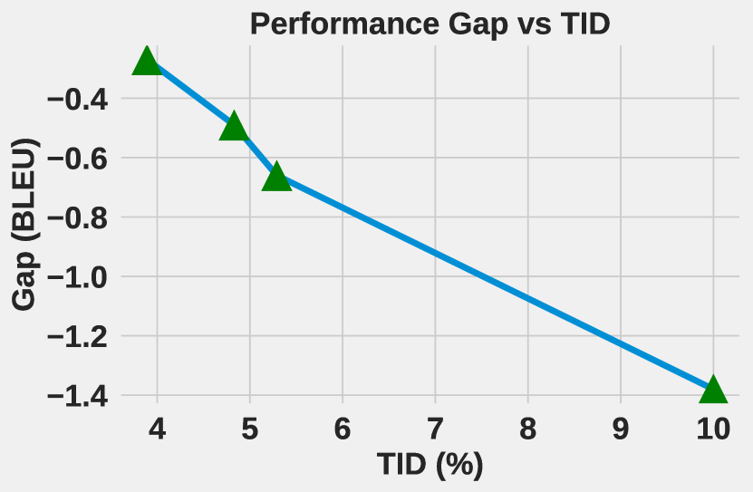
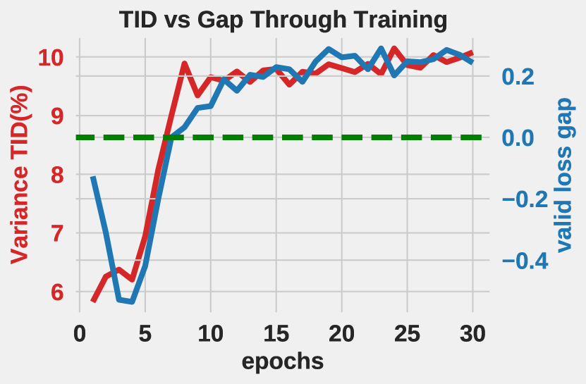
Figure 3: Left: Variance TID and BLEU gap between $\text{Transformer}_{BN}$ and $\text{Transformer}_{LN}$ when replacing different numbers of LN layers with BN. Right: Variance TID and valid loss gap of Post-Norm Transformer through training.

We compute the TID of the last BN layer in Table 1 and leave the average TID of all BN layers in Appendix D. The last BN layer, which is close to the output, significantly impacts the model prediction. We observe that TID is highly correlated with the performance gap between BN and LN. When TID is large, e.g., on WMT16, BN performs much worse than LN. However, when the TID of BN is negligible, e.g., on PTB and WT103, BN performs better than LN with a large margin. We select one dataset from each task with Pre-Norm Transformer and define the total TID as the sum of mean and variance TID. At the end of the training, the total TID of the last BN layer for WMT16/CoNLL/IMDB/WT103 is around 38%/16%/9%/5%, and the performance gap is -2.1 BLEU scores/-1.1 F1 score/-0.1% accuracy/6.8 perplexity (PPL). Larger TID tends to hurt BN’s performance.

To explore the quantitative relation between TID and performance gap, we substitute $L=3\sim 6$ LN layers with BN layers from the bottom in the Post-Norm Transformer encoder on IWSLT14. As $L$ increases, the variance TID of the last BN layer grows, and the BLEU scores of $\text{Transformer}_{BN}$ drops off. We plot the variance TID and BLEU gap between $\text{Transformer}_{BN}$ and $\text{Transformer}_{LN}$ in Figure 3 (left). We can see that the two quantities are highly correlated.

In Figure 3 (right), we plot the variance TID of the last BN layer and the validation loss gap between $\text{Transformer}_{BN}$ and $\text{Transformer}_{LN}$ on IWSLT14 through training. The validation loss gap is calculated by subtracting loss of $\text{Transformer}_{LN}$ from $\text{Transformer}_{BN}$. At the beginning of training, BN performs better than LN. When the TID begins to explode, BN’s performance starts to degrade.

Based on the results in Table 1 and observations in Figure 3, we argue that TID serves as an indicator of BN’s performance in Transformers. Large TID hurts BN’s performance, while BN with small TID performs better than LN due to its more efficient optimization (see experimental validation in Section 4.3).

4 Suppressing High TID by RBN

In this section, we are devoted to reducing the TID of BN when it is large. If TID is suppressed, the performance of BN will be improved and may exceed LN due to the training efficiency of BN.

4.1 Regularized Batch Normalization

Assume there are $H$ layers of BN in a neural network. We denote the batch statistics and running statistics of each layer by $\mu_{B}^{i}$, $\sigma_{B}^{i}$, and $\mu^{i}$, $\sigma^{i}$, $i=1\ldots,H$. Assume the Cross-Entropy (CE) loss with respect to the neural network parameters $\theta$ is denoted by ${\cal L}(\theta)$. To avoid undesirable training inference discrepancy, we pose the optimization as a constrained problem:

$$\min\limits_{\theta} {\cal L}(\theta)$$ (6)

$$s.t. \mathbb{E}_{p_{B}}d_{\mu}(\mu_{B}^{i},\mu^{i})\leq\epsilon_{i},\ i=1,\ldots,H$$

$$\mathbb{E}_{p_{B}}d_{\sigma}(\sigma_{B}^{i},\sigma^{i})\leq\eta_{i},\ i=1,\ldots,H$$

where $d_{\mu}$ and $d_{\sigma}$ measure the inconsistency of mean and variance. This is equivalent to

$$\min\limits_{\theta}\quad{\cal L}(\theta)+\sum\limits_{i=1}^{H}\lambda_{i}\mathbb{E}d_{\mu}(\mu_{B}^{i},\mu^{i})+\nu_{i}\mathbb{E}d_{\sigma}(\sigma_{B}^{i},\sigma^{i})$$ (7)

To simplify the problem, we set $\lambda_{i}=\lambda$, $\nu_{i}=\nu$, for $\ i=1,\ldots,H$.
When handling batch data, we apply gradient-based optimization to the following loss (${\cal L}_{B}(\theta)$ is the batch CE loss):

$${\cal L}_{B}(\theta)+\sum\limits_{i=1}^{H}\lambda d_{\mu}(\mu_{B}^{i},\mu^{i})+\nu d_{\sigma}(\sigma_{B}^{i},\sigma^{i})$$

In particular, we choose $d_{\mu}\left(\mu_{B},\mu\right)=\|\mu_{B}-\mu\|_{2}^{2}$ and $d_{\sigma}\left(\sigma_{B},\sigma\right)=\|\sigma_{B}-\sigma\|_{2}^{2}$. The sensitivity analysis of hyperparameter is given in Section 4.3. Since back propagating through the running statistics $\mu$ and $\sigma$ would trace back to the first batch of data which is impractical, we simply stop the gradient of $\mu$ and $\sigma$ in back propagation.

4.2 Experimental Result for RBN

Table 2: Results for the performance of Post-Norm (top) and Pre-Norm (bottom) Transformers with LN/BN/RBN. RBN consistently improves BN and could match or exceed LN on 17 out of 20 settings.

Task	NMT (+)		LM (-)		NER (+)		TextCls (+)
Datasets	IWSLT14	WMT16	PTB	WT103	Resume	CoNLL	IMDB	Sogou	DBPedia	Yelp
Post-LN	35.5	27.3	53.2	20.9	94.8	91.3	84.1	94.6	97.5	93.3
Post-BN	34.0	25.0	45.9	17.2	94.5	90.9	84.0	94.3	97.5	93.3
Post-RBN	35.5	26.5	44.6	17.1	94.8	91.4	84.5	94.7	97.6	93.6
Pre-LN	35.5	27.3	54.5	24.6	94.0	91.0	84.1	94.5	97.5	93.3
Pre-BN	34.8	25.2	45.9	17.8	93.2	89.9	84.0	94.3	97.5	93.3
Pre-RBN	35.6	26.2	43.2	17.1	94.0	90.6	84.4	94.7	97.5	93.5

We choose $\lambda,\nu$ both from $\left\{0,0.01,0.1,1\right\}$ by validation loss. Results are shown in Table 2. The optimal hyperparameters are listed in Appendix B.

Neural Machine Translation

On IWSLT14 datasets, we see that RBN significantly improves BN and can exceed LN with 0.1 BLEU scores with Pre-Norm Transformer and match LN with Post-Norm Transformer. On WMT16 dataset, although RBN still falls behind LN, it could improve 1.5/1.0 BLEU scores over BN in Post-Norm/Pre-Norm setting. The reason is that even though RBN can suppress a large amount of TID, the remaining is still large since the original TID is huge. We speculate that the high data diversity in WMT16 contributes to the explosive TID of BN, which is hard to remove. We leave the verification as future work.

Language Modeling

On Post-Norm Transformer, BN could boost the testing PPL of LN from 53.2 to 45.9 on PTB and from 20.9 to 17.2 on WikiText-103. Furthermore, substituting RBN for BN improves the testing PPL to 44.6 on PTB and 17.1 on WikiText-103. On Pre-Norm Transformer, BN elevates the testing PPL of LN from 54.5 to 45.9 on PTB and from 24.6 to 17.8 on WikiText-103. Moreover, replacing BN with RBN improves the testing PPL to 43.2 on PTB and 17.1 on WikiText-103. Overall, RBN exceeds LN with 8.6/3.8 testing PPL with Post-Norm Transformer and 11.3/7.5 testing PPL with Pre-Norm Transformer on PTB/WikiText-103.

Named Entity Recognition

BN performs worse than LN on both Resume and CoNLL2003 datasets, especially for Pre-Norm Transformer. RBN improves BN in all settings, matches or exceeds LN in three out of four settings. By taking the better performance of Post-Norm and Pre-Norm, RBN matches the performance of LN on Resume and exceeds LN on CoNLL2003.

Text Classification

We find that BN performs similar to/worse than LN on 4/4 settings. RBN improves the performance of BN consistently and can match/exceed LN on 1/7 settings. RBN improves BN with 0.3% accuracy on average, which shows the benefit of our regularization. We do not intend to achieve the state-of-the-art performance but to verify the efficacy of RBN.

Comparison to BN’s Variants

We compare our RBN with Power Normalization (PN) [38], Batch Renormalization (BRN) [16], and Moving Averaing Batch Normaliazation (MABN) [47] in Table 3. These methods incorporate population statistics of BN in training, which is beneficial for alleviating training inference inconsistency of BN. PN and MABN are implemented by their official codes. BRN is implemented according to their paper [16]. The configurations of PN, BRN, and MABN are given in Appendix F. We highlight that PN incorporates layer scaling (LS) [51], which is important for stabilizing training, as shown in the supplementary materials and official code of PN. We thus report the results for PN only and PN with layer scaling (PN+LS). We can see that RBN performs the best in most settings. PN and MABN is not stable without layer scaling, especially for Post-Norm Transformers.

Table 3: Results for the performance of Post-Norm (top) and Pre-Norm (bottom) Transformers with PN/BRN/MABN/RBN.

Task	NMT (+)		LM (-)		NER (+)		TextCls (+)
Datasets	IWSLT14	WMT16	PTB	WT103	Resume	CoNLL	IMDB	Sogou	DBPedia	Yelp
Post-PN-only	0	0	254.6	inf	94.4	67.1	84.2	90.6	97.1	89.6
Post-PN+LS	35.6	0	49.8	21.0	94.3	90.9	84.0	94.6	97.4	93.2
Post-BRN	35.3	25.8	45.1	17.3	93.6	89.9	83.6	94.5	97.5	93.3
Post-MABN	0	0	47.4	33.6	94.4	90.8	84.1	94.5	97.5	93.5
Post-RBN	35.5	26.5	44.6	17.1	94.8	91.4	84.5	94.7	97.6	93.6
Pre-PN-only	34.5	26.0	48.6	inf	5.0	11.1	84.2	94.4	97.4	93.3
Pre-PN+LS	35.6	27.2	59.8	20.9	93.3	54.1	83.3	94.4	97.3	93.4
Pre-BRN	35.2	25.3	45.7	17.5	94.1	91.1	84.3	94.5	97.4	93.4
Pre-MABN	35.0	26.8	48.7	inf	94.8	90.9	84.4	94.6	97.5	93.3
Pre-RBN	35.6	26.2	43.2	17.1	94.0	90.6	84.4	94.7	97.5	93.5

4.3 Analysis

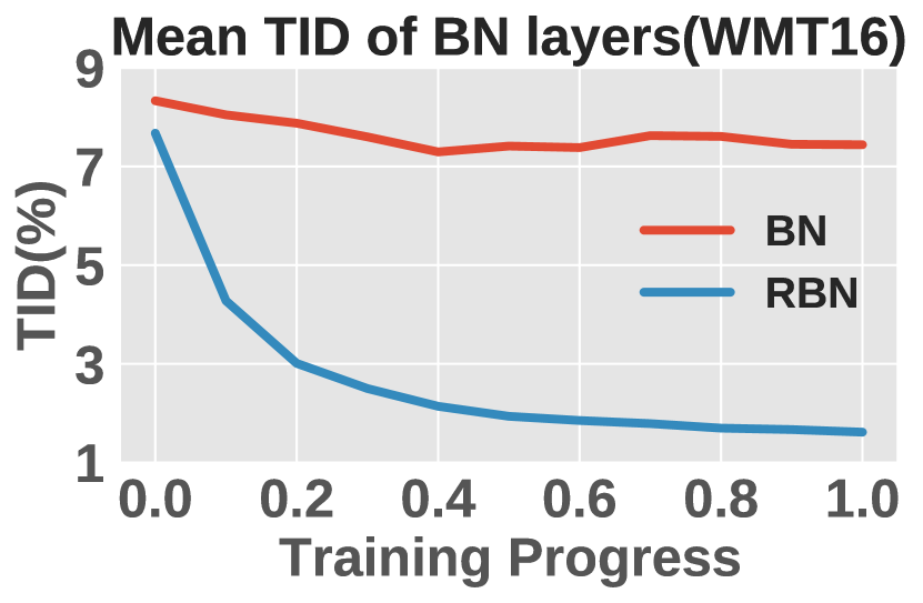
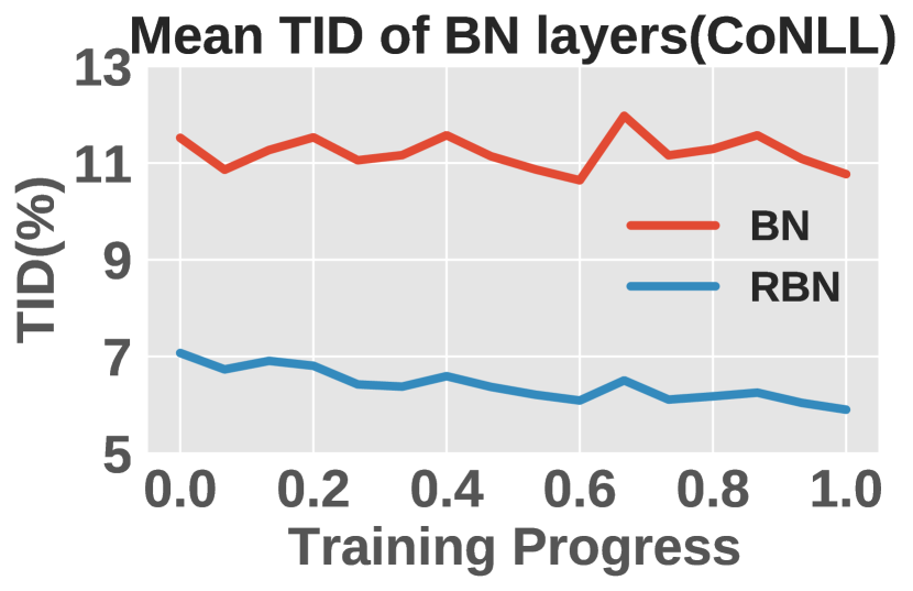
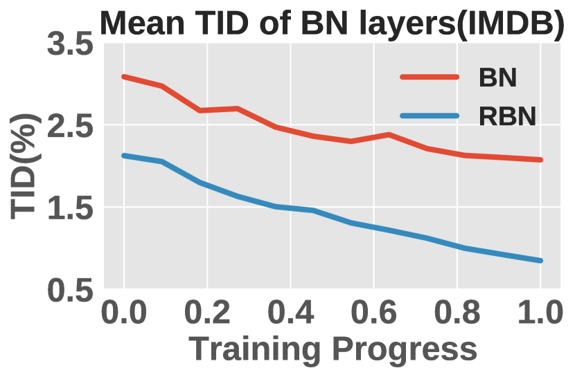
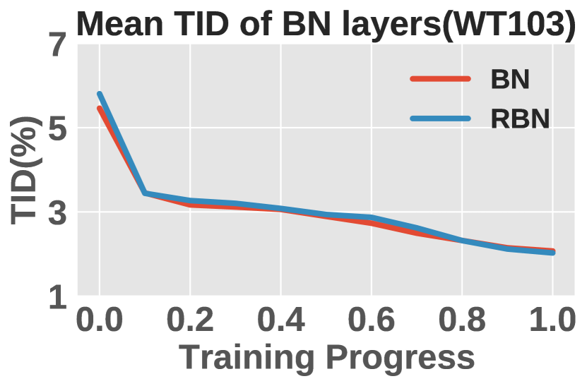
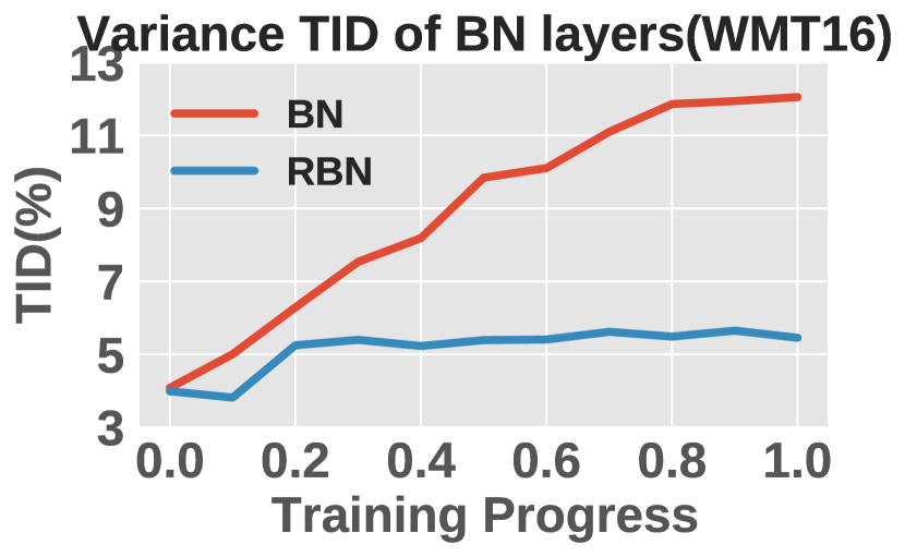
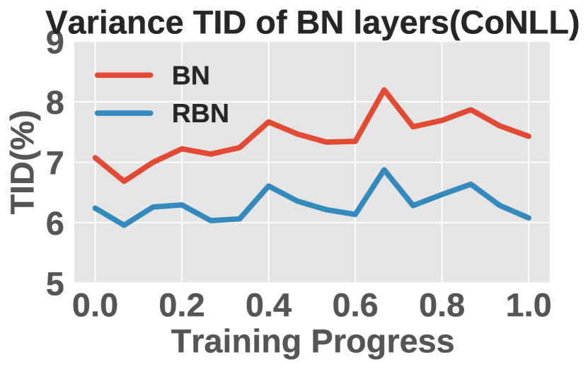
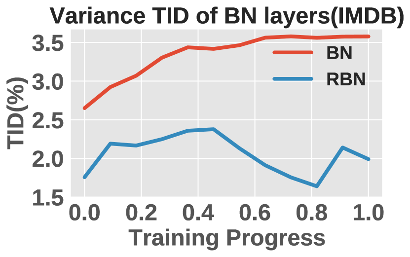
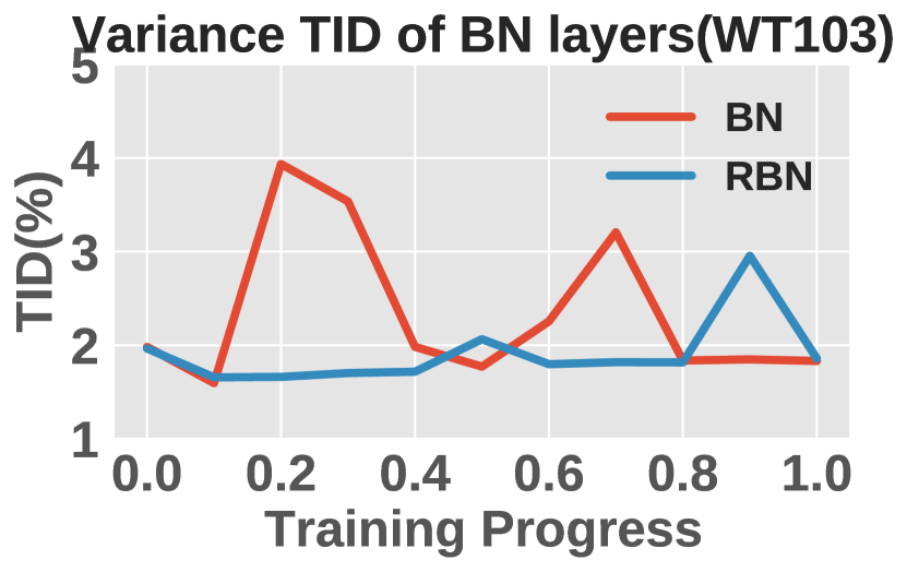
Figure 4: Average Mean and Variance TID on WMT16/CoNLL/IMDB/WT103 for Pre-Norm Transformer with BN and RBN. RBN reduces the Mean and Variance TID of BN at the end of the training and leads to better performance.

Training Inference Inconsistency

Table 4: TID of the last BN/RBN layer in Post-Norm and Pre-Norm Transformers on various NLP tasks. RBN reduces the TID of BN effectively.

Task	NMT		LM		NER		TextCls
Datasets	IWSLT14	WMT16	PTB	WT103	Resume	CoNLL	IMDB	Sogou	DBPedia	Yelp
Post-Norm Transformer
Mean TID of $\text{BN}_{last}$	1.5%	4.2%	0.9%	1.8%	1.7%	4.2%	1.8%	1.8%	2.2%	3.1%
Mean TID of $\text{RBN}_{last}$	0.8%	2.3%	0.9%	1.8%	1.4%	1.9%	0.2%	0.2%	0.3%	0.2%
Var TID of $\text{BN}_{last}$	10.6%	17.9%	1.1%	2.0%	3.7%	9.5%	3.9%	4.3%	3.5%	4.0%
Var TID of $\text{RBN}_{last}$	6.7%	7.7%	1.1%	1.7%	3.0%	5.0%	1.2%	0.2%	0.3%	0.1%
Pre-Norm Transformer
Mean TID of $\text{BN}_{last}$	3.4%	7.9%	1.6%	2.4%	9.6%	10.0%	2.9%	7.5%	3.9%	12.1%
Mean TID of $\text{RBN}_{last}$	3.2%	1.3%	1.6%	2.4%	4.5%	4.0%	0.7%	1.0%	1.1%	1.0%
Var TID of $\text{BN}_{last}$	4.6%	30.1%	1.7%	2.5%	6.5%	6.4%	6.2%	7.1%	3.3%	8.6%
Var TID of $\text{RBN}_{last}$	1.5%	12.1%	1.7%	2.4%	6.3%	5.6%	4.7%	0.4%	0.5%	0.5%

We compute the TID of the last BN layer ($\text{BN}_{last}$) in Table 4 and plot the average TID of BN and RBN on WMT16, WT103, CoNLL2003, and IMDB datasets for Pre-Norm Transformers through training in Figure 4. Figures of TID for other datasets and Post-Norm Transformer can be found in Appendix C. We can see that RBN reduces BN’s mean and variance TID at the end of training. On neural machine translation and named entity recognition tasks, the original TID is large. RBN significantly decreases the TID of BN and improves BN’s performance by a clear margin. For language modeling and text classification tasks, RBN also reduces the moderate TID of BN and gets better PPL or accuracy.

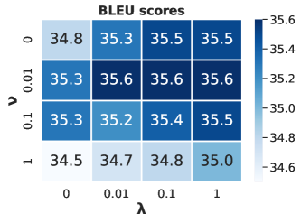
Figure 5: The BLEU scores on IWSLT14 with different mean ($\lambda$) and variance ($\nu$) discrepancy penalty of RBN.

Sensitivity to Hyperparameters

We test different penalty coefficients for RBN on neural machine translation with Pre-Norm Transformer. The results are shown in Figure 5. Penalizing the mean and variance discrepancy can both improve the performance of BN. Combining them with moderate coefficients achieves the best performance.

Training Dynamics

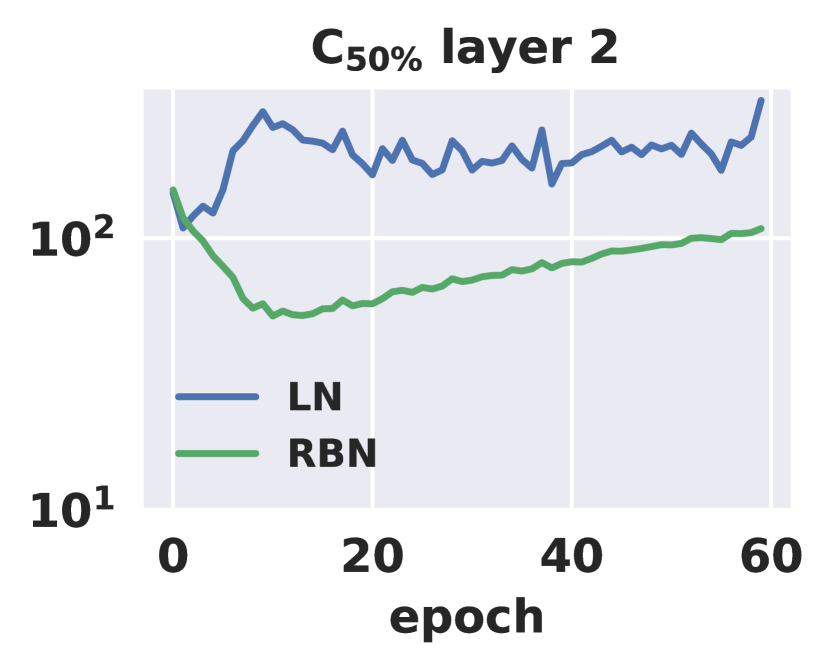
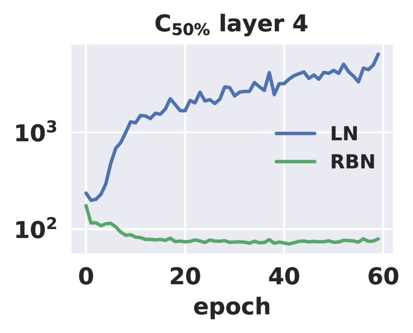
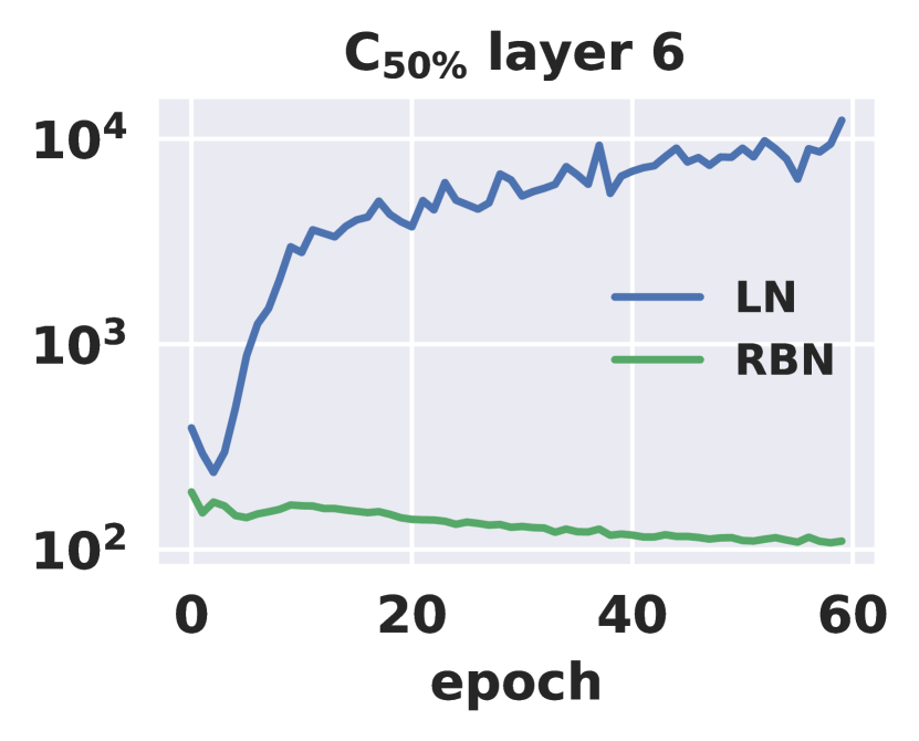
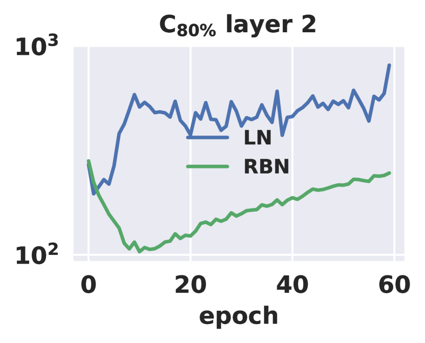
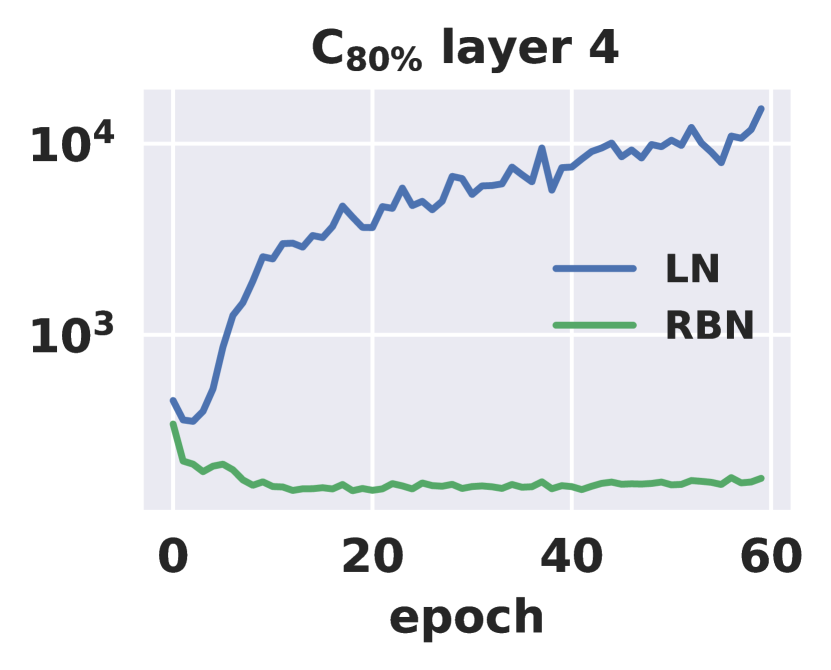
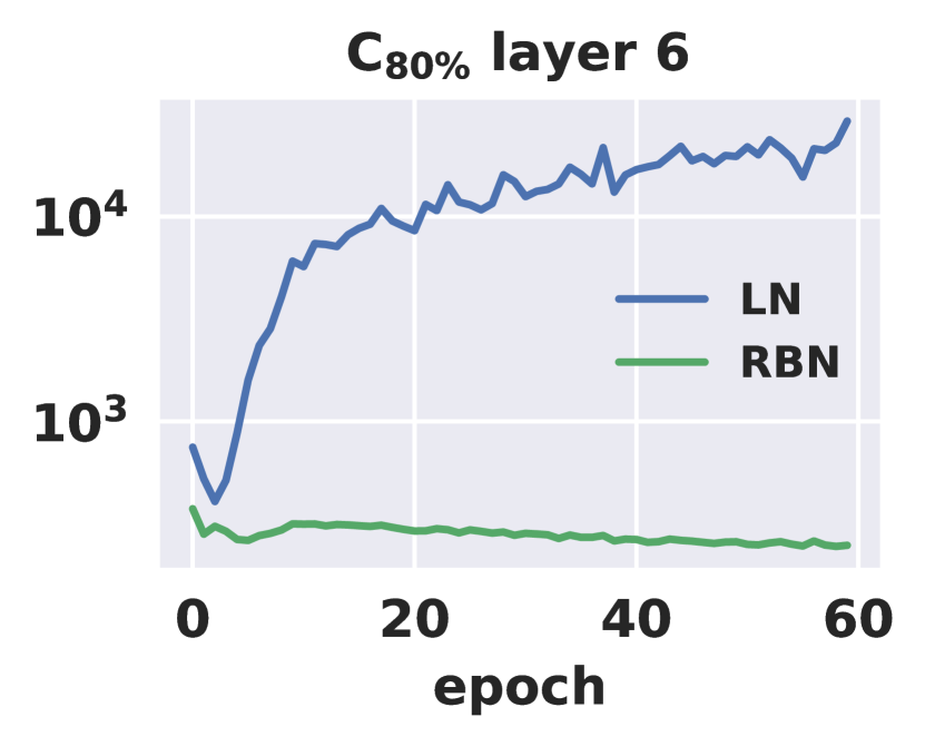
Figure 6: $C_{50\%}$ (top), and $C_{80\%}$ (bottom) of input features of Transformer encoder layer 2/4/6. RBN improves the $C_{50\%}$ and $C_{80\%}$ of LN, especially for deep layers (2 orders of magnitude at layer 6).

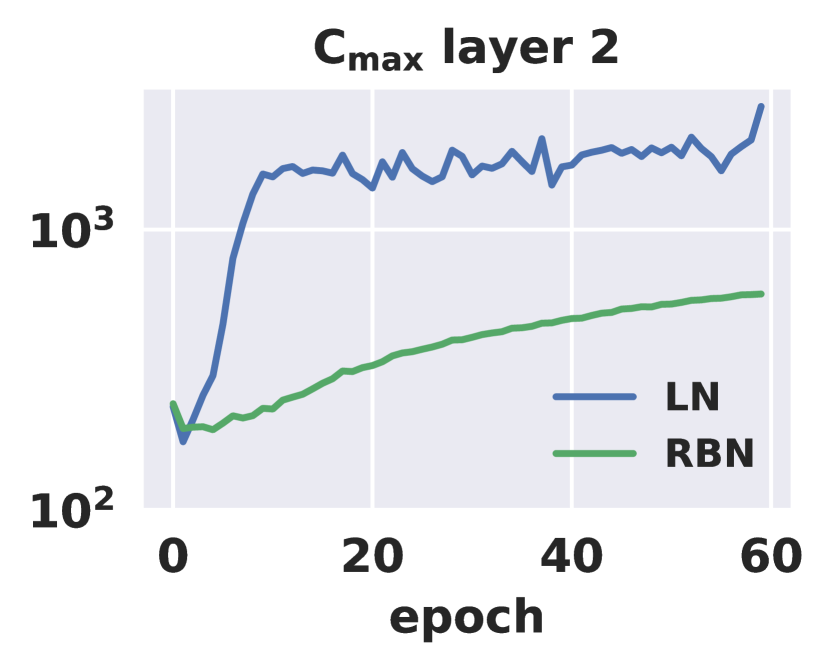
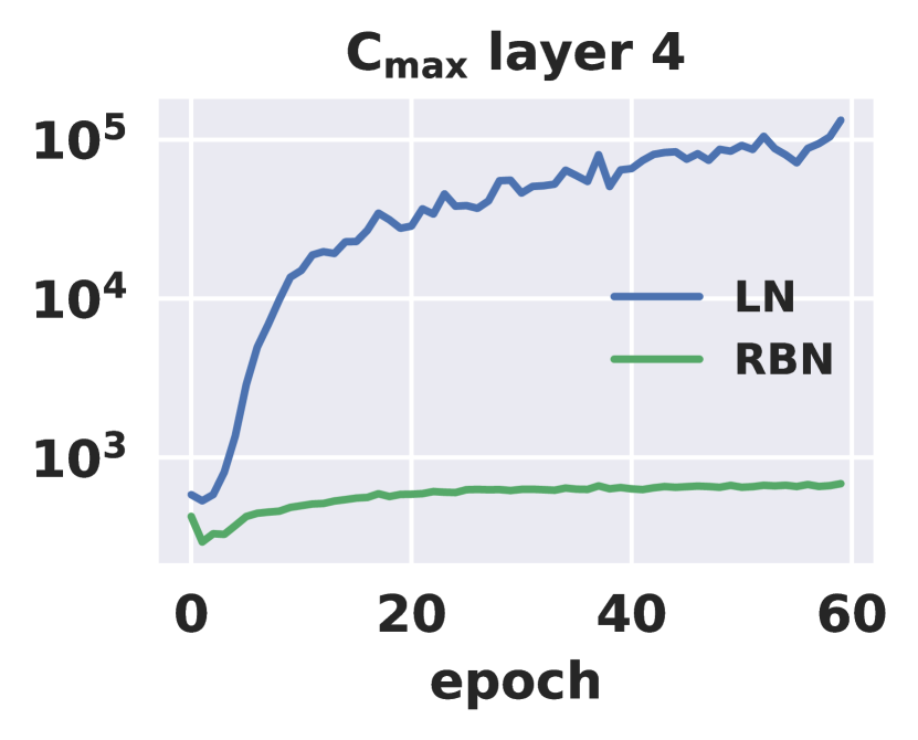
Figure 7: $\text{C}_{max}$ of input features of Transformer encoder layer 2/4/6 through training.

To show the optimization advantages of RBN over LN, we explore the layer-wise training dynamics of LN and RBN in Pre-Norm Transformer on IWSLT14. We refer the reader to Huang et al. [13] for detailed analysis about the correlation between optimization of neural network and layer-wise training dynamics. We empirically observe that replacing LN with RBN significantly improves the layer-wise conditioning [13] of Transformer. We denote the intermediate embedding in Transformer by $\tilde{\mathbf{X}}\in\mathbb{R}^{B\times T\times d}$, each $\tilde{\mathbf{X}}_{i,j,:}\in\mathbb{R}^{d}$ is a word vector. We reshape $\tilde{\mathbf{X}}$ to a sequence of word vectors to $\mathbf{X}=\left[\mathbf{x}_{1},\mathbf{x}_{2},\ldots,\mathbf{x}_{BT}\right]\in\mathbb{R}^{BT\times d}$. We assume $BT>d$ which is satisfied in our experiments. We define the general condition number with respect to the percentage as $C_{p}(\mathbf{X})=\frac{\sigma_{1}}{\sigma_{\lceil pd\rceil}}$, $0<p\leq 1$. $\lceil a\rceil$ is the smallest integer that is larger than or equal to $a$. Lower $C_{p}(\mathbf{X})$ is usually associated with faster convergence of training. We plot $C_{50\%}$, and $C_{80\%}$ of input features of transformer encoder layer 2/4/6 in Figure 6. We can see that RBN significantly reduces the $C_{50\%}$ and $C_{80\%}$ of LN, usually with orders of magnitude. We also plot the layer-wise $C_{max}(\mathbf{X})=\lambda_{max}((\mathbf{X}^{T}\mathbf{X})^{\frac{1}{2}})$ in Figure 7. Smaller $C_{max}$ usually permits higher learning rates which leads to faster training and better generalization [11]. RBN has much smaller $C_{max}$ than LN.

5 Conclusion and Limitation

In this paper, we defined Training Inference Discrepancy (TID) and showed that TID is a good indicator of BN’s performance for Transformers, supported by comprehensive experiments. We observed BN performs much better than LN when TID is negligible and proposed Regularized BN (RBN) to alleviate TID when TID is large. Our RBN has theoretical advantages in optimization and works empirically better by controlling the TID of BN when compared with LN. We hope our work will facilitate a better understanding and application of BN in NLP.

Limitation.

Our analyses on TID are almost empirical studies without theoretical guarantee. It is better to further model the geometric distribution of word embedding, evolving along with the training dynamics and information propagation, with theoretical derivation under mild assumptions. Besides, our proposed RBN cannot entirely suppress huge TID in training large-scale datasets with high diversity, leading to degraded performance. One possible direction is to combine RBN and LN for both better optimization properties and small TID, as explored in [14, 48] for CV tasks.

Acknowledgement

Ji Wu was sponsored by National Key Research & Development Program of China (2021ZD0113402), Tsinghua University Spring Breeze Fund (2021Z99CFZ010), National Key Research & Development Program of China (Grant Number: 2021YFC2500803), and Tsinghua-Toyota Joint Research Institute Inter-disciplinary Program. Lei Huang was supported by National Natural Science Foundation of China (Grant No. 62106012) and the Fundamental Research Funds for the Central Universities.

Appendix A Experimental Details

In the main paper, we sketch the experimental settings. Here, we report the details. Our WMT16 experiments require two NVIDIA 3090 GPUs with 24GB memory each, and other experiments are implemented with one NVIDIA 3090 GPU.

Neural Machine Translation

Datasets

We use two widely used datasets: IWSLT14 German-to-English (De-En) dataset and WMT16 English-to-German (En-De) dataset. IWSLT14/WMT16 contains 0.15M/4.5M sentence pairs.

Configurations

Our code is based on fairseq [32]. We use six encoder layers and six decoder layers for both datasets. We keep the Transformer decoder unchanged and only modify normalization layers in Transformer encoder throughout NMT experiments. We follow the model settings in [38] for IWSLT14 and apply $\text{Transformer}_{base}$ model [41] for WMT16. At test phase, we averaged the last six checkpoints and measure case sensitive tokenized BLEU [33] with beam size 4/5 and length penalty 0.6/1.0 for ISWLT14/WMT16. We use Adam with $\left(\beta_{1},\beta_{2}\right)=\left(0.9,0.98\right)$, an inverse square root learning rate scheduler, and a warmup stage with $8000$ steps. We apply labeling smoothing $\epsilon_{ls}=0.1$. For IWSLT14, we set num-tokens=4096, max-epochs=60, dropout=0.3, attention dropout=0.1, activation dropout=0.1 and lr=$5e^{-4}$/$1.5e^{-3}$ for Post-Norm/Pre-Norm Transformer. For WMT16, we set num-tokens=8192, update-freq=4, max-epochs=20, dropout=0.1, attention dropout=0.1, activation dropout=0.1 and lr=$7e^{-4}$/$2e^{-3}$ for Post-Norm/Pre-Norm Transformer.

Language Modeling

Datasets

We conduct experiments on PTB (0.93M tokens) [30] and WikiText-103 (WT103)(100M tokens) [29]. We follow the evaluation scheme in [7] and use perplexity (PPL) of test set to compare the model performance.

Configurations

Following the experimental settings in [38][26], we use three and six layers tensorized transformer core-1 for PTB and Wikitext-103 separately. We use the same hyperparameters for Post-Norm and Pre-Norm Transformer. We use Adam optimizer and set lr=$2.5e^{-4}$ with linear decay. For PTB, we use dropout=0.3, batch size=120, max-steps=20000. For PTB, we use dropout=0.1, batch size=60, max-steps=200000.

Named Entity Recognition

Datasets

We choose two widely used NER datasets: CoNLL2003 (English) [35] and Resume (Chinese) [52]. CoNLL2003/Resume contains four/eight kinds of named entities. CoNLL2003 contains 14.0k/3.2k/3.5k sentences for train/dev/test split while Resume includes 3.8k/0.5k/0.5k sentences for train/dev/test set. We use F1 score to measure the model performance.

Configurations

We mainly follow the experimental settings in [46]. We use two and four layers transformer encoder for CoNLL2003 and Resume, respectively. An additional CRF layer [15] is added to model the transition probability. We use SGD optimizer with 0.9 momentum and 1% total steps as warmup steps. We set the learning rate to be $9e^{-4}$ and $7e^{-4}$ for CoNLL2003 and Resume.

Text Classification

Datasets

For text classification, we use the code and most configurations in [3]. We select one small scale dataset (IMDB [27]) and three large scale datasets (Yelp, DBPedia, Sogou News), including two sentiment classification tasks (IMDB, Yelp) and two topic classification tasks (DBPedia, Sogou News).

Configurations

We use six Transformer encoder layers with a CLS token at the beginning of each sentence for classification. We extract 30% of training data as validation set for all datasets. The best checkpoint for the validation is applied in the test phase. We run three times with different random seeds for each setting and report the mean accuracy.

Appendix B Optimal Hyperparameters

For RBN, we choose $\lambda,\nu$ both from $\left\{0,0.01,0.1,1\right\}$ by validation loss. We empirically find that increasing the mean penalty on NMT for Post-Norm Transformer can further improve the BLEU scores. Thus, we apply $\left(\lambda,\nu\right)=\left(10,0\right)/\left(100,0\right)$ on ISWLT14/WMT16 for Post-Norm Transformer exceptionally.

Table 5: Optimal hyperparameters $\left(\lambda,\nu\right)$ for each experimental setting. $\left(\lambda,\nu\right)$ are mean and variance penalty coefficients separately.

Task	NMT		LM		NER		TextCls
Datasets	IWSLT14	WMT16	PTB	WT103	Resume	CoNLL	IMDB	Sogou	DBPedia	Yelp
Post-Norm	(10,0)	(100,0)	(0.1,0.01)	(0.1,0.01)	(0.01,0)	(0.01,0)	(0.1,0)	(0.1,0.01)	(0.1,0.01)	(0,0.1)
Pre-Norm	(0.1,0.01)	(0.1,0)	(0.01,0)	(0.1,0)	(0.01,0)	(0.01,0)	(0,0.01)	(0.1,0.01)	(0.1,0.01)	(0.1,0.01)

Appendix C Average TID of BN and RBN

In the main paper, we have shown the TID of the last BN (RBN) layer on various NLP datasets with Post-Norm or Pre-Norm Transformer. Here, we report the average TID of all BN (RBN) layers (Table 6). RBN decreases the average TID of BN.

Table 6: Average TID of all BN/RBN layer in Post-Norm and Pre-Norm Transformers on various natural language tasks at the end of training. RBN reduces the TID of BN effectively.

Task	NMT		LM		NER		TextCls
Datasets	IWSLT14	WMT16	PTB	WT103	Resume	CoNLL	IMDB	Sogou	DBPedia	Yelp
Post-Norm Transformer
Mean TID of BN_avg	2.8%	3.0%	1.0%	0.9%	5.0%	9.9%	1.5%	1.9%	1.3%	2.7%
Mean TID of RBN_avg	0.8%	1.5%	1.0%	1.0%	4.4%	5.6%	0.4%	0.4%	0.4%	0.4%
Var TID of BN_avg	7.1%	4.9%	1.1%	2.2%	4.2%	9.8%	3.1%	2.1%	1.4%	3.9%
Var TID of RBN_avg	2.6%	2.8%	1.0%	1.0%	4.0%	6.5%	1.7%	0.3%	0.3%	0.2%
Pre-Norm Transformer
Mean TID of BN_avg	3.2%	7.6%	1.6%	2.1%	10.3%	10.8%	2.1%	4.2%	2.5%	4.2%
Mean TID of RBN_avg	3.0%	1.6%	1.6%	2.0%	6.7%	5.9%	0.8%	1.2%	1.2%	1.1%
Var TID of BN_avg	5.5%	12.8%	1.6%	1.9%	8.1%	7.4%	3.6%	3.7%	2.1%	5.1%
Var TID of RBN_avg	1.6%	5.6%	1.6%	1.8%	7.5%	6.1%	1.9%	0.5%	0.5%	0.5%

Appendix D Figures of TID Through Training

We have shown the average mean and variance TID on WMT16/CoNLL/IMDB/WT103 for Pre-Norm Transformer with BN and RBN in the main paper. Here, we plot the average mean and variance TID on other datasets with Pre-Norm and Post-Norm Transformers in Figures 8, 9, 10 and 11. RBN reduces the TID of BN effectively.

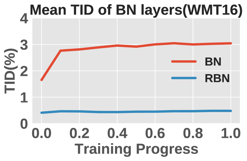
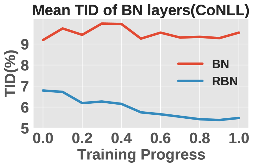
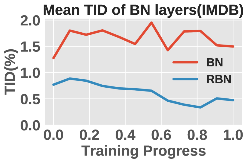
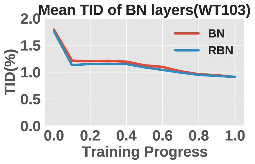
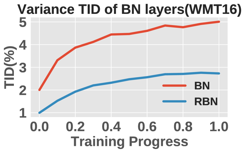
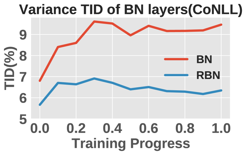
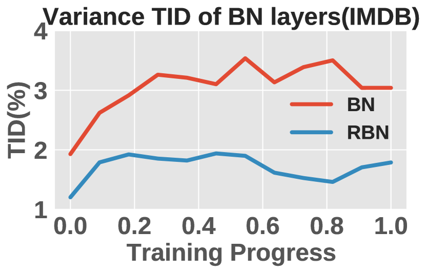
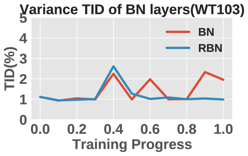
Figure 8: Averaged Mean and Variance TID on WMT16/CoNLL/IMDB/WT103 for Post-Norm Transformer with BN and RBN.

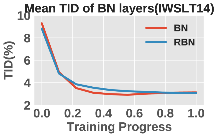
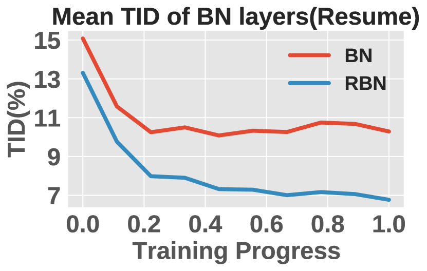
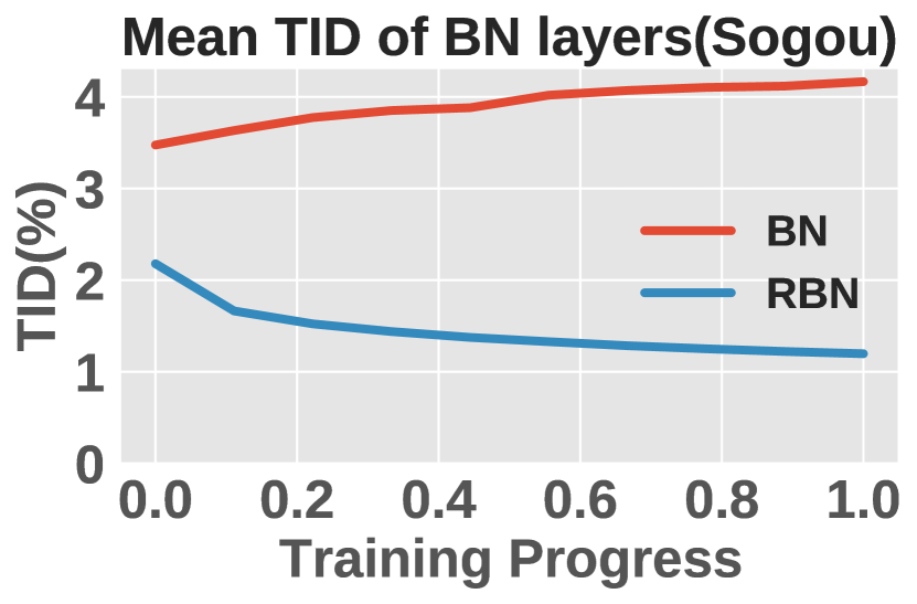
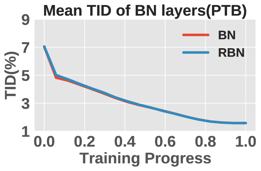
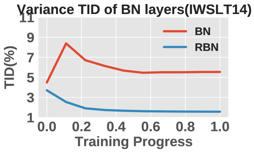
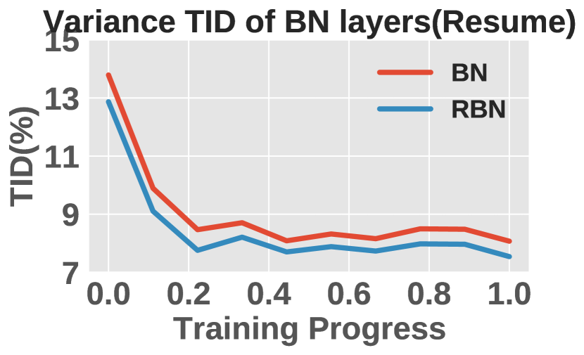
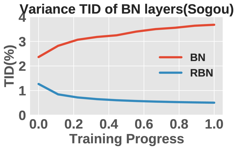
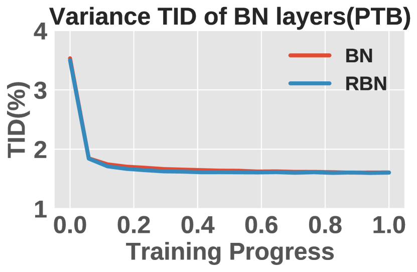
Figure 9: Averaged Mean and Variance TID on IWSLT14/Resume/Sogou/PTB for Pre-Norm Transformer with BN and RBN.

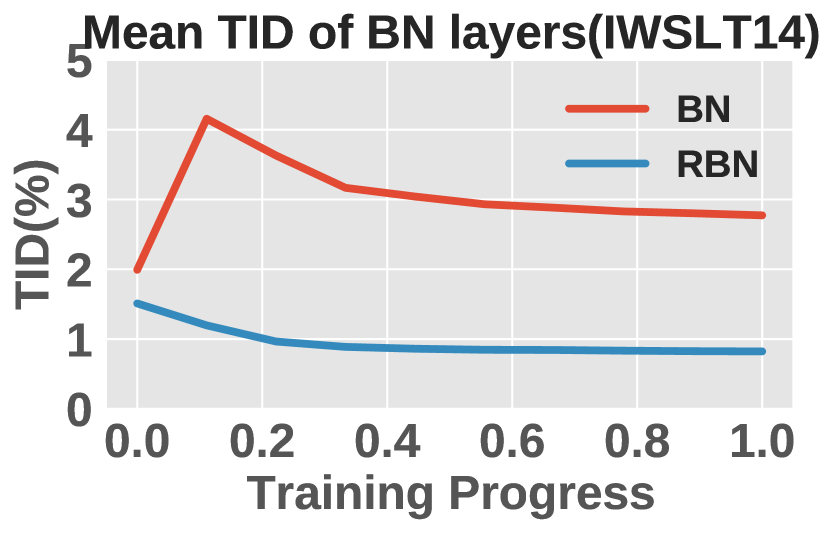
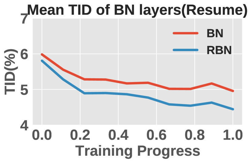
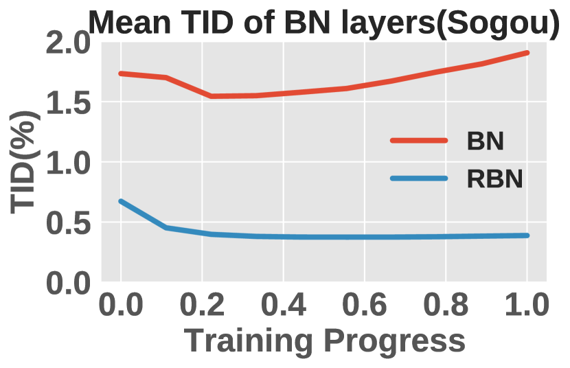
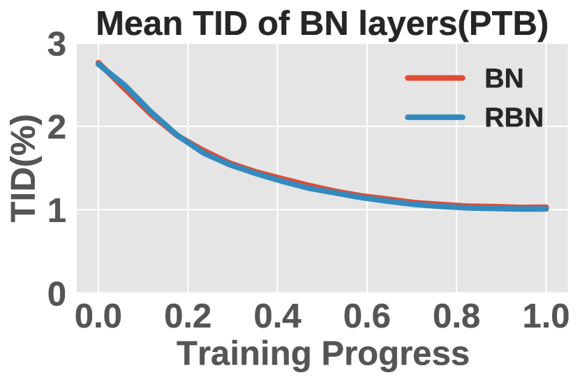
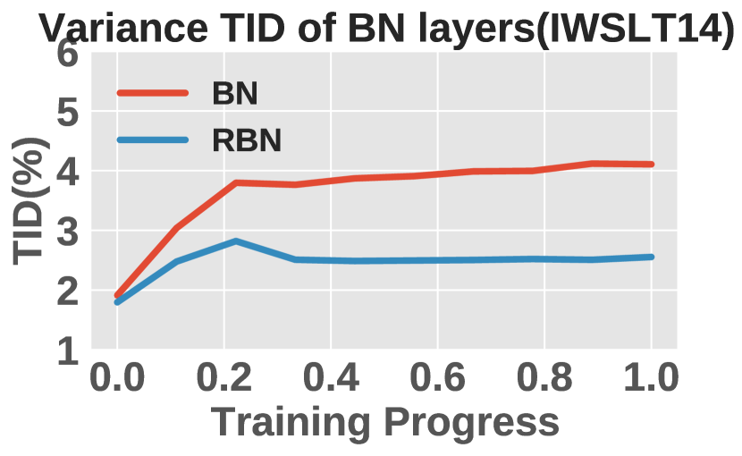
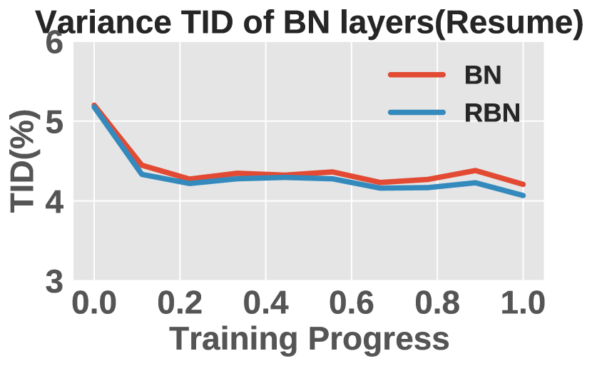
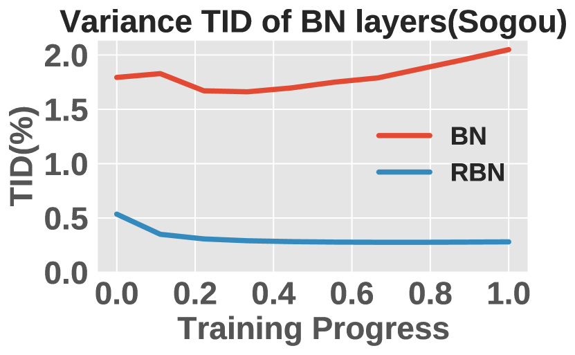
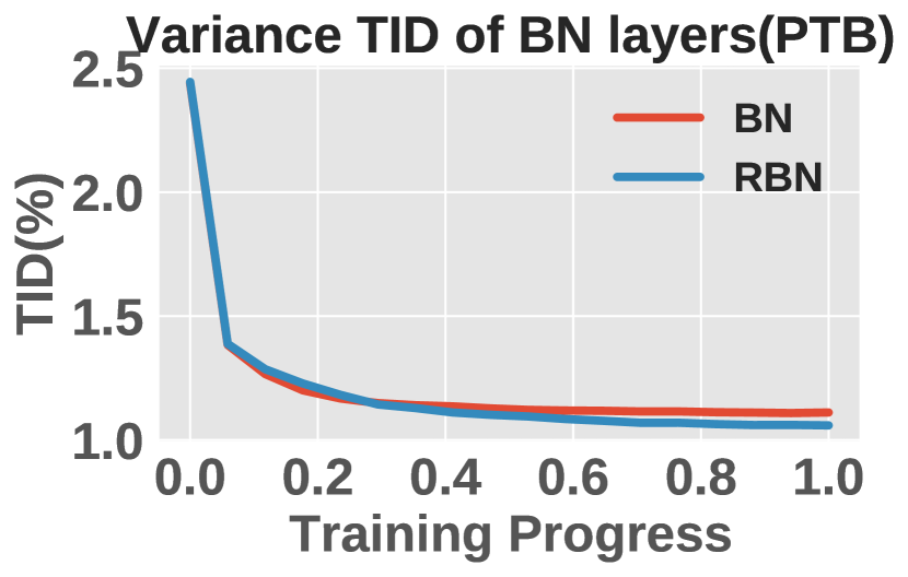
Figure 10: Averaged Mean and Variance TID on IWSLT14/Resume/Sogou/PTB for Post-Norm Transformer with BN and RBN.

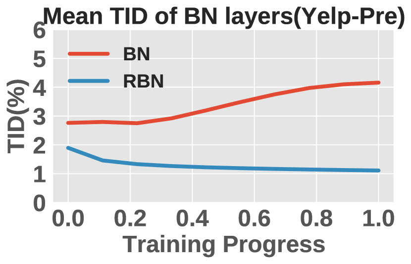
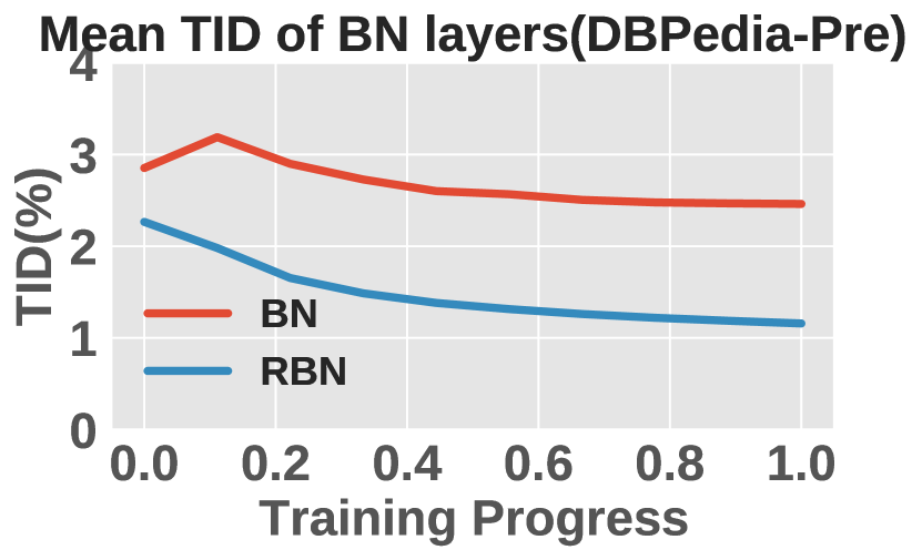
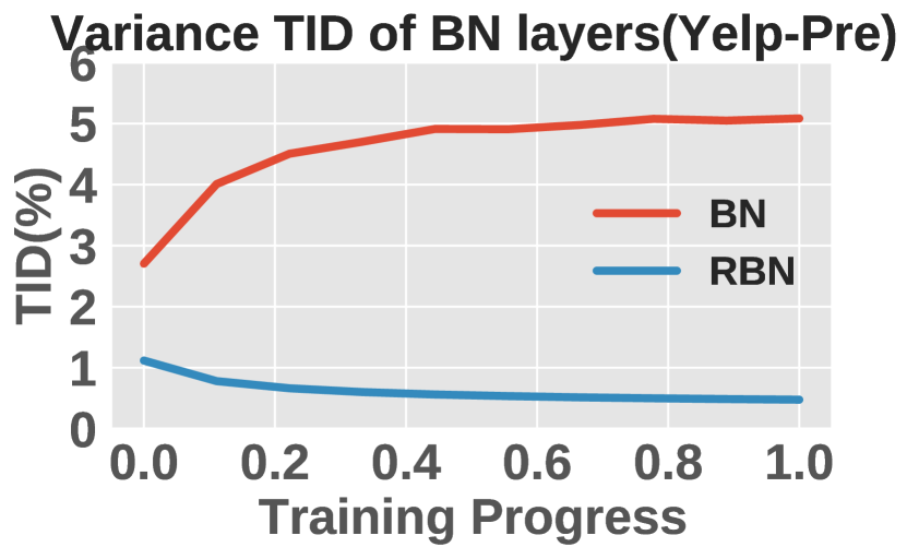
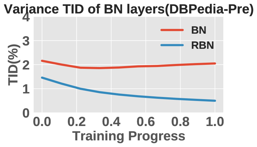
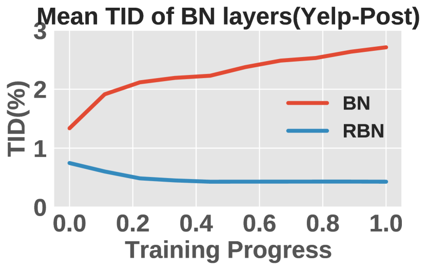
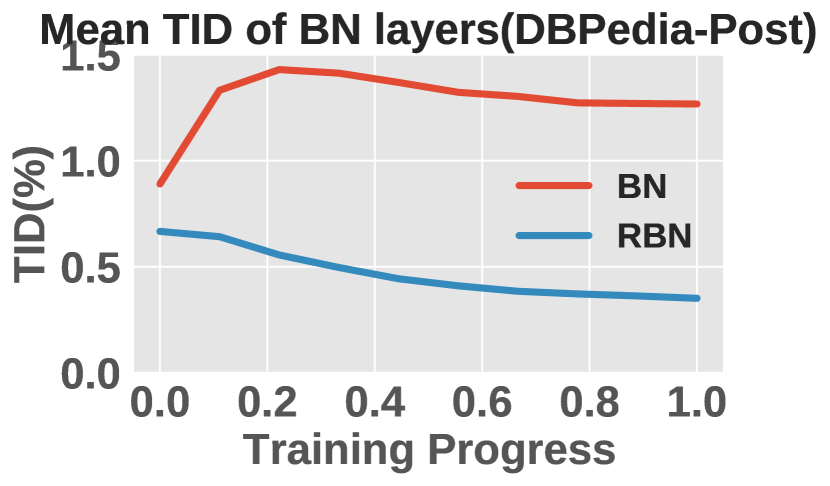
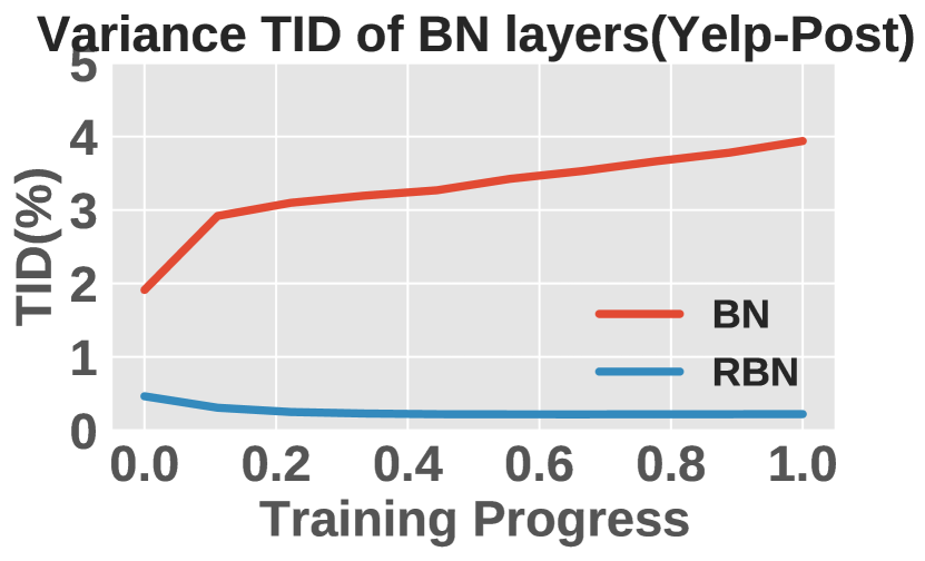
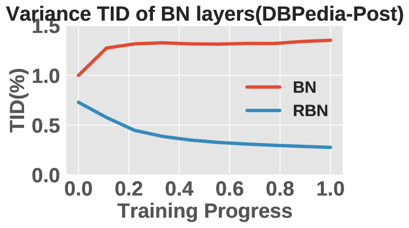
Figure 11: Averaged Mean and Variance TID on Yelp/DBPedia for Pre-Norm Transformer (upper) and Post-Norm Transformer (bottom) with BN and RBN.

Appendix E Other settings of BN in Test Stage

In the main paper, we test BN (RBN) with population statistics estimated by Exponential Moving Average (EMA). Here, we test two other settings of BN on IWSLT14 dataset. In the first setting (Table 7), we reestimate the population statistics of BN by running two more epochs with zero learning rate. In the second setting (Table 8), we test BN with batch statistics of different effective batch size (max-tokens).

From Table 7, we can see that reestimating the population statistics leads to similar results as EMA. However, using batch statistics instead of population statistics boosts the performance of Post-Norm $\text{Transformer}_{BN}$, but hurts the performance of Pre-Norm $\text{Transformer}_{BN}$ and Post-Norm $\text{Transformer}_{RBN}$ (Table 8). Pre-Norm $\text{Transformer}_{RBN}$ is robust to different max-tokens. Note that $\text{Transformer}_{LN}$ achieves 35.5 BLEU in both Pre-Norm and Post-Norm settings. BN can not match the performance of LN by changing the test settings.

Table 7: EMA: Use population statistics estimated by EMA. Reestimation: Run two more epochs with zero learning rate to update population statistics. The performance metric is BLEU.

	Post-BN	Post-RBN	Pre-BN	Pre-RBN
EMA	34.0	35.5	34.8	35.6
Reestimation	33.8	35.6	34.9	35.4

Appendix F Configurations of BN’s Variants

We compare the performance of RBN with Power Normalization (PN) [38], Batch Renormalization (BRN) [16] and Moving Averaing Batch Normaliazation (MABN) [47] in the main paper. We mainly follow the hyperparameters in their papers. For PN, we use 4000 warmups, and set foward and backward momentum as $0.9$. For BRN, we use one epoch BN as warmup and linearly increase $r$ to 3 and $d$ to 5. $r$ and $d$ are renormalizing factors. For MABN, we use $16$ mini-batches to compute simple moving average statistics and momentum $\alpha=0.98$ to compute exponential moving average statistics.

Appendix G Potential Negative Societal Impact

We spend many GPU hours on running experiments which may negatively impact the environment.

Table 8: Testing BN (RBN) with batch statistics of different max-tokens.

Max-tokens	Post-BN	Post-RBN	Pre-BN	Pre-RBN
EMA	34.0	35.5	34.8	35.6
512	34.8	34.9	27.2	35.6
1024	35.1	34.9	30.9	35.6
2048	35.2	34.9	32.3	35.6
4096	35.2	34.9	32.7	35.6
8192	35.2	34.9	32.8	35.6
16384	35.2	34.8	32.9	35.6

References

- Ba et al. [2016] Jimmy Lei Ba, Jamie Ryan Kiros, and Geoffrey E. Hinton. Layer normalization, 2016.
- Benz et al. [2021] Philipp Benz, Chaoning Zhang, Adil Karjauv, and In So Kweon. Revisiting batch normalization for improving corruption robustness. In WACV, 2021.
- Bhardwaj et al. [2021] Rishabh Bhardwaj, Navonil Majumder, Soujanya Poria, and Eduard Hovy. More identifiable yet equally performant transformers for text classification. In Proceedings of the 59th Annual Meeting of the Association for Computational Linguistics and the 11th International Joint Conference on Natural Language Processing (Volume 1: Long Papers), pages 1172–1182. Association for Computational Linguistics, 2021.
- Bjorck et al. [2018] Nils Bjorck, Carla P Gomes, Bart Selman, and Kilian Q Weinberger. Understanding batch normalization. In S. Bengio, H. Wallach, H. Larochelle, K. Grauman, N. Cesa-Bianchi, and R. Garnett, editors, Advances in Neural Information Processing Systems, volume 31. Curran Associates, Inc., 2018.
- Brown et al. [2020] Tom Brown, Benjamin Mann, Nick Ryder, Melanie Subbiah, Jared D Kaplan, Prafulla Dhariwal, Arvind Neelakantan, Pranav Shyam, Girish Sastry, Amanda Askell, Sandhini Agarwal, Ariel Herbert-Voss, Gretchen Krueger, Tom Henighan, Rewon Child, Aditya Ramesh, Daniel Ziegler, Jeffrey Wu, Clemens Winter, Chris Hesse, Mark Chen, Eric Sigler, Mateusz Litwin, Scott Gray, Benjamin Chess, Jack Clark, Christopher Berner, Sam McCandlish, Alec Radford, Ilya Sutskever, and Dario Amodei. Language models are few-shot learners. In Advances in Neural Information Processing Systems, volume 33, pages 1877–1901. Curran Associates, Inc., 2020.
- Chiley et al. [2019] Vitaliy Chiley, Ilya Sharapov, Atli Kosson, Urs Koster, Ryan Reece, Sofia Samaniego de la Fuente, Vishal Subbiah, and Michael James. Online normalization for training neural networks. In NeurIPS, 2019.
- Dai et al. [2019] Zihang Dai, Zhilin Yang, Yiming Yang, Jaime Carbonell, Quoc Le, and Ruslan Salakhutdinov. Transformer-XL: Attentive language models beyond a fixed-length context. In Proceedings of the 57th Annual Meeting of the Association for Computational Linguistics, pages 2978–2988. Association for Computational Linguistics, 2019.
- Daneshmand et al. [2020] Hadi Daneshmand, Jonas Moritz Kohler, Francis Bach, Thomas Hofmann, and Aurélien Lucchi. Batch normalization provably avoids ranks collapse for randomly initialised deep networks. In NeurIPS, 2020.
- Daneshmand et al. [2021] Hadi Daneshmand, Amir Joudaki, and Francis Bach. Batch normalization orthogonalizes representations in deep random networks. In Advances in Neural Information Processing Systems, 2021.
- Devlin et al. [2019] Jacob Devlin, Ming-Wei Chang, Kenton Lee, and Kristina Toutanova. BERT: Pre-training of deep bidirectional transformers for language understanding. In Proceedings of the 2019 Conference of the North American Chapter of the Association for Computational Linguistics: Human Language Technologies, Volume 1 (Long and Short Papers), pages 4171–4186. Association for Computational Linguistics, 2019.
- Hardt et al. [2016] Moritz Hardt, Benjamin Recht, and Yoram Singer. Train faster, generalize better: Stability of stochastic gradient descent. ArXiv, abs/1509.01240, 2016.
- Huang et al. [2019] Lei Huang, Yi Zhou, Fan Zhu, Li Liu, and Ling Shao. Iterative normalization: Beyond standardization towards efficient whitening. 2019 IEEE/CVF Conference on Computer Vision and Pattern Recognition (CVPR), pages 4869–4878, 2019.
- Huang et al. [2020] Lei Huang, Jie Qin, Li Liu, Fan Zhu, and Ling Shao. Layer-wise conditioning analysis in exploring the learning dynamics of dnns. In Andrea Vedaldi, Horst Bischof, Thomas Brox, and Jan-Michael Frahm, editors, Computer Vision – ECCV 2020, pages 384–401. Springer International Publishing, 2020. ISBN 978-3-030-58536-5.
- Huang et al. [2022] Lei Huang, Yi Zhou, Tian Wang, Jie Luo, and Xianglong Liu. Delving into the estimation shift of batch normalization in a network. arXiv preprint arXiv:2203.10778, 2022.
- Huang et al. [2015] Zhiheng Huang, Wei Xu, and Kai Yu. Bidirectional lstm-crf models for sequence tagging. ArXiv, abs/1508.01991, 2015.
- Ioffe [2017] Sergey Ioffe. Batch renormalization: Towards reducing minibatch dependence in batch-normalized models. In NeurIPS, 2017.
- Ioffe and Szegedy [2015] Sergey Ioffe and Christian Szegedy. Batch normalization: Accelerating deep network training by reducing internal covariate shift. In Proceedings of the 32nd International Conference on Machine Learning, volume 37 of Proceedings of Machine Learning Research, pages 448–456. PMLR, 2015.
- Izmailov et al. [2018] Pavel Izmailov, Dmitrii Podoprikhin, Timur Garipov, Dmitry Vetrov, and Andrew Gordon Wilson. Averaging weights leads to wider optima and better generalization. arXiv preprint arXiv:1803.05407, 2018.
- Krizhevsky [2009] Alex Krizhevsky. Learning multiple layers of features from tiny images. 2009.
- Krizhevsky et al. [2012] Alex Krizhevsky, Ilya Sutskever, and Geoffrey E. Hinton. Imagenet classification with deep convolutional neural networks. In NIPS, pages 1106–1114, 2012.
- LeCun et al. [2015] Yann LeCun, Yoshua Bengio, and Geoffrey Hinton. Deep learning. Nature, 521(7553):436–444, 2015.
- Li et al. [2019] Xiang Li, Shuo Chen, Xiaolin Hu, and Jian Yang. Understanding the disharmony between dropout and batch normalization by variance shift. In Proceedings of the IEEE/CVF Conference on Computer Vision and Pattern Recognition (CVPR), June 2019.
- Li et al. [2016] Yanghao Li, Naiyan Wang, Jianping Shi, Jiaying Liu, and Xiaodi Hou. Revisiting batch normalization for practical domain adaptation. arXiv preprint arXiv:1603.04779, 2016.
- Luo et al. [2019a] Ping Luo, Jiamin Ren, Zhanglin Peng, Ruimao Zhang, and Jingyu Li. Differentiable learning-to-normalize via switchable normalization. In ICLR, 2019a.
- Luo et al. [2019b] Ping Luo, Xinjiang Wang, Wenqi Shao, and Zhanglin Peng. Towards understanding regularization in batch normalization. In International Conference on Learning Representations, 2019b.
- Ma et al. [2019] Xindian Ma, Peng Zhang, Shuai Zhang, Nan Duan, Yuexian Hou, Ming Zhou, and Dawei Song. A tensorized transformer for language modeling. In H. Wallach, H. Larochelle, A. Beygelzimer, F. d'Alché-Buc, E. Fox, and R. Garnett, editors, Advances in Neural Information Processing Systems, volume 32. Curran Associates, Inc., 2019.
- Maas et al. [2011] Andrew L. Maas, Raymond E. Daly, Peter T. Pham, Dan Huang, Andrew Y. Ng, and Christopher Potts. Learning word vectors for sentiment analysis. In Proceedings of the 49th Annual Meeting of the Association for Computational Linguistics: Human Language Technologies, pages 142–150. Association for Computational Linguistics, 2011.
- Martens and Grosse [2015] James Martens and Roger B. Grosse. Optimizing neural networks with kronecker-factored approximate curvature. CoRR, abs/1503.05671, 2015.
- Merity et al. [2016] Stephen Merity, Caiming Xiong, James Bradbury, and Richard Socher. Pointer sentinel mixture models. CoRR, abs/1609.07843, 2016.
- Mikolov et al. [2011] Tomas Mikolov, Anoop Deoras, Stefan Kombrink, Lukas Burget, and Jan "Honza" Cernocky. Empirical evaluation and combination of advanced language modeling techniques. In Interspeech. ISCA, August 2011.
- Nado et al. [2020] Zachary Nado, Shreyas Padhy, D Sculley, Alexander D’Amour, Balaji Lakshminarayanan, and Jasper Snoek. Evaluating prediction-time batch normalization for robustness under covariate shift. arXiv preprint arXiv:2006.10963, 2020.
- Ott et al. [2019] Myle Ott, Sergey Edunov, Alexei Baevski, Angela Fan, Sam Gross, Nathan Ng, David Grangier, and Michael Auli. fairseq: A fast, extensible toolkit for sequence modeling. In Proceedings of the 2019 Conference of the North American Chapter of the Association for Computational Linguistics (Demonstrations), pages 48–53. Association for Computational Linguistics, 2019.
- Papineni et al. [2002] Kishore Papineni, Salim Roukos, Todd Ward, and Wei-Jing Zhu. Bleu: A method for automatic evaluation of machine translation. In Proceedings of the 40th Annual Meeting on Association for Computational Linguistics, ACL ’02, page 311–318. Association for Computational Linguistics, 2002.
- Radford et al. [2019] Alec Radford, Jeff Wu, Rewon Child, David Luan, Dario Amodei, and Ilya Sutskever. Language models are unsupervised multitask learners. 2019.
- Sang and Meulder [2003] Erik Tjong Kim Sang and Fien De Meulder. Introduction to the conll-2003 shared task: Language-independent named entity recognition. In CoNLL, 2003.
- Santurkar et al. [2018] Shibani Santurkar, Dimitris Tsipras, Andrew Ilyas, and Aleksander Madry. How does batch normalization help optimization? In S. Bengio, H. Wallach, H. Larochelle, K. Grauman, N. Cesa-Bianchi, and R. Garnett, editors, Advances in Neural Information Processing Systems, volume 31, 2018.
- Schneider et al. [2020] Steffen Schneider, Evgenia Rusak, Luisa Eck, Oliver Bringmann, Wieland Brendel, and Matthias Bethge. Improving robustness against common corruptions by covariate shift adaptation. In NeurIPS, 2020.
- Shen et al. [2020] Sheng Shen, Zhewei Yao, Amir Gholami, Michael Mahoney, and Kurt Keutzer. Powernorm: Rethinking batch normalization in transformers. In ICML, 2020.
- Singh and Shrivastava [2019] Saurabh Singh and Abhinav Shrivastava. Evalnorm: Estimating batch normalization statistics for evaluation. In ICCV, 2019.
- Summers and Dinneen [2020] Cecilia Summers and Michael J. Dinneen. Four things everyone should know to improve batch normalization. In ICLR, 2020.
- Vaswani et al. [2017] Ashish Vaswani, Noam Shazeer, Niki Parmar, Jakob Uszkoreit, Llion Jones, Aidan N Gomez, Ł ukasz Kaiser, and Illia Polosukhin. Attention is all you need. In I. Guyon, U. V. Luxburg, S. Bengio, H. Wallach, R. Fergus, S. Vishwanathan, and R. Garnett, editors, Advances in Neural Information Processing Systems, volume 30. Curran Associates, Inc., 2017.
- Wu and He [2018] Yuxin Wu and Kaiming He. Group normalization. In ECCV, 2018.
- Wu and Johnson [2021] Yuxin Wu and Justin Johnson. Rethinking "batch" in batchnorm. CoRR, abs/2105.07576, 2021.
- Xiong et al. [2020] Ruibin Xiong, Yunchang Yang, Di He, Kai Zheng, Shuxin Zheng, Chen Xing, Huishuai Zhang, Yanyan Lan, Liwei Wang, and Tie-Yan Liu. On layer normalization in the transformer architecture. In ICML 2020, 2020.
- Xu et al. [2019] Jingjing Xu, Xu Sun, Zhiyuan Zhang, Guangxiang Zhao, and Junyang Lin. Understanding and improving layer normalization. In Advances in Neural Information Processing Systems, volume 32, 2019.
- Yan et al. [2019] Hang Yan, Bocao Deng, Xiaonan Li, and Xipeng Qiu. Tener: Adapting transformer encoder for named entity recognition, 2019.
- Yan et al. [2020] Junjie Yan, Ruosi Wan, Xiangyu Zhang, Wei Zhang, Yichen Wei, and Jian Sun. Towards stabilizing batch statistics in backward propagation of batch normalization. In ICLR, 2020.
- Yao et al. [2021a] Zhuliang Yao, Yue Cao, Yutong Lin, Ze Liu, Zheng Zhang, and Han Hu. Leveraging batch normalization for vision transformers. 2021 IEEE/CVF International Conference on Computer Vision Workshops (ICCVW), pages 413–422, 2021a.
- Yao et al. [2021b] Zhuliang Yao, Yue Cao, Shuxin Zheng, Gao Huang, and Stephen Lin. Cross-iteration batch normalization. In CVPR, 2021b.
- Yong et al. [2020] Hongwei Yong, Jianqiang Huang, Xiansheng Hua, and Lei Zhang. Gradient centralization: A new optimization technique for deep neural networks. In ECCV, 2020.
- Zhang and Sennrich [2019] Biao Zhang and Rico Sennrich. Root mean square layer normalization. In H. Wallach, H. Larochelle, A. Beygelzimer, F. d'Alché-Buc, E. Fox, and R. Garnett, editors, Advances in Neural Information Processing Systems, volume 32. Curran Associates, Inc., 2019.
- Zhang and Yang [2018] Yue Zhang and Jie Yang. Chinese ner using lattice lstm. In ACL, 2018.