Markup-to-Image Diffusion Models
with Scheduled Sampling

Abstract

Building on recent advances in image generation, we present a fully data-driven approach to rendering markup into images. The approach is based on diffusion models, which parameterize the distribution of data using a sequence of denoising operations on top of a Gaussian noise distribution. We view the diffusion denoising process as a sequential decision making process, and show that it exhibits compounding errors similar to exposure bias issues in imitation learning problems. To mitigate these issues, we adapt the scheduled sampling algorithm to diffusion training. We conduct experiments on four markup datasets: mathematical formulas (LaTeX), table layouts (HTML), sheet music (LilyPond), and molecular images (SMILES). These experiments each verify the effectiveness of the diffusion process and the use of scheduled sampling to fix generation issues. These results also show that the markup-to-image task presents a useful controlled compositional setting for diagnosing and analyzing generative image models.

1 Introduction

Recent years have witnessed rapid progress in text-to-image generation with the development and deployment of pretrained image/text encoders (Radford et al., 2021; Raffel et al., 2020) and powerful generative processes such as denoising diffusion probabilistic models (Sohl-Dickstein et al., 2015; Ho et al., 2020). Most existing image generation research focuses on generating realistic images conditioned on possibly ambiguous natural language (Nichol et al., 2021; Saharia et al., 2022; Ramesh et al., 2022). In this work, we instead study the task of markup-to-image generation, where the presentational markup describes exactly one-to-one what the final image should look like.

While the task of markup-to-image generation can be accomplished with standard renderers, we argue that this task has several nice properties for acting as a benchmark for evaluating and analyzing text-to-image generation models. First, the deterministic nature of the problem enables exposing and analyzing generation issues in a setting with known ground truth. Second, the compositional nature of markup language is nontrivial for neural models to capture, making it a challenging benchmark for relational properties. Finally, developing a model-based markup renderer enables interesting applications such as markup compilers that are resilient to typos, or even enable mixing natural and structured commands (Glennie, 1960; Teitelman, 1972).

We build a collection of markup-to-image datasets shown in Figure 1: mathematical formulas, table layouts, sheet music, and molecules (Nienhuys & Nieuwenhuizen, 2003; Weininger, 1988). These datasets can be used to assess the ability of generation models to produce coherent outputs in a structured environment. We then experiment with utilizing diffusion models, which represent the current state-of-the-art in conditional generation of realistic images, on these tasks.

The markup-to-image challenge exposes a new class of generation issues. For example, when generating formulas, current models generate perfectly formed output, but often generate duplicate or misplaced symbols (see Figure 2). This type of error is similar to the widely studied exposure bias issue in autoregressive text generation (Ranzato et al., 2015). To help the model fix this class of errors during the generation process, we propose to adapt scheduled sampling (Bengio et al., 2015). Specifically, we train diffusion models by using the model’s own generations as input such that the model learns to correct its own mistakes.

Experiments on all four datasets show that the proposed scheduled sampling approach improves the generation quality compared to baselines, and generates images of surprisingly good quality for these tasks. Models produce clearly recognizable images for all domains, and often do very well at representing the semantics of the task. Still, there is more to be done to ensure faithful and consistent generation in these difficult deterministic settings. All models, data, and code are publicly available at https://github.com/da03/markup2im.

Math

⬇

\widetilde \gamma _ { \mathrm { h o p f } } \simeq \sum _ { n > 0 } \widetilde { G } _ { n } { \frac { ( - a ) ^ { n } } { 2 ^ { 2 n - 1 } } }

Table Layouts

⬇

... <span style=" font-weight:bold; text-align:center; font-size:150%; " > f j </span> </div> ...

Sheet Music

⬇

\relative c’’ { \time 4/4 d4 | r2 b4 b2 | ces4 b4~ g2 f4 | a4 d8 | e4 g16 g2 f2 r4 | des2 d8 d8 f8 e4 d8 a16 b16 | d4 e2 d2. a8~ g4 r16~ e16. d2 f4 b4 e2 | f4. | b16 a16 e4. r2~ c4 r4 b4 d8 b2 | d4 | r8. e8 e2 | r8~ e2 }

Molecules

⬇

COc1ccc(cc1N)C(=O)Nc2ccccc2

Figure 1: Markup-to-Image suite with generated images. Tasks include mathematical formulas (LaTeX), table layouts (HTML), sheet music (LilyPond), and molecular images (SMILES). Each example is conditioned on a markup (bottom) and produces a rendered image (top). Evaluation directly compares the rendered image with the ground truth image.

2 Motivation: Diffusion Models for Markup-to-Image Generation

Task

We define the task of markup-to-image generation as converting a source in a markup language describing an image to that target image. The input is a sequence of $M$ tokens $x=x_{1},\cdots,x_{M}\in\mathcal{X}$, and the target is an image $y\in\mathcal{Y}\subseteq\mathbb{R}^{H\times W}$ of height $H$ and width $W$ (for simplicity we only consider grayscale images here). The task of rendering is defined as a mapping $f:\mathcal{X}\to\mathcal{Y}$. Our goal is to approximate the rendering function using a model parameterized by $\theta$ $f_{\theta}:\mathcal{X}\to\mathcal{Y}$ trained on supervised examples $\{(x^{i},y^{i}):i\in\{1,2,\cdots,N\}\}$. To make the task tangible, we show several examples of $x,y$ pairs in Figure 1.

Challenge

The markup-to-image task contains several challenging properties that are not present in other image generation benchmarks. While the images are much simpler, they act more discretely than typical natural images. Layout mistakes by the model can lead to propagating errors throughout the image. For example, including an extra mathematical symbol can push everything one line further down. Some datasets also have long-term symbolic dependencies, which may be difficult for non-sequential models to handle, analogous to some of the challenges observed in non-autoregressive machine translation (Gu et al., 2018).

Generation with Diffusion Models

Denoising diffusion probabilistic models (DDPM) (Ho et al., 2020) parameterize a probabilistic distribution $P(y_{0}|x)$ as a Markov chain $P(y_{t-1}|y_{t})$ with an initial distribution $P(y_{T})$. These models conditionally generate an image by sampling iteratively from the following distribution (we omit the dependence on $x$ for simplicity):

$$P(y_{T})=\mathcal{N}(0,I)$$

$$P(y_{t-1}|y_{t})=\mathcal{N}(\mu_{\theta}(y_{t},t);\sigma_{t}^{2}I)$$

where $y_{1},y_{2},\cdots,y_{T}$ are latent variables of the same size as $y_{0}\in\mathcal{Y}$, $\mu_{\theta}(\cdot,t)$ is a neural network parameterizing a map $\mathcal{Y}\to\mathcal{Y}$.

Diffusion models have proven to be effective for generating realistic images (Nichol et al., 2021; Saharia et al., 2022; Ramesh et al., 2022) and are more stable to train than alternative approaches for image generation such as Generative Adversarial Networks (Goodfellow et al., 2014). Diffusion models are surprisingly effective on the markup-to-image datasets as well. However, despite generating realistic images, they make major mistakes in the layout and positioning of the symbols. For an example of these mistakes see Figure 2 (left).

We attribute these mistakes to error propagation in the sequential Markov chain. Small mistakes early in the sampling process can lead to intermediate $y_{t}$ states that may have diverged significantly far from the model’s observed distribution during training. This issue has been widely studied in the inverse RL and autoregressive token generation literature, where it is referred to as exposure bias (Ross et al., 2011; Ranzato et al., 2015).

$150$

$250$

$350$

$450$

$550$

$650$

$750$

$1000$

Figure 2: The generation process of diffusion (left) versus diffusion+schedule sampling (right). The numbers on the y-axis are the number of diffusion steps ($T-t$). The ground truth LaTeX is γ_n^μ=α_n^μ+~α_n^μ,   n≠0.—

3 Scheduled Sampling for Diffusion Models

In this work, we adapt scheduled sampling, a simple and effective method based on DAgger (Ross et al., 2011; Bengio et al., 2015) from discrete autoregressive models to the training procedure of diffusion models. The core idea is to replace the standard training procedure with a biased sampling approach that mimics the test-time model inference based on its own predictions. Before describing this approach, we first give a short background on training diffusion models.

Background: Training Diffusion Models

Diffusion models maximize an evidence lower bound (ELBO) on the above Markov chain. We introduce an auxiliary Markov chain $Q(y_{1},\cdots,y_{T}|y_{0})=\prod_{t=1}^{T}Q(y_{t}|y_{t-1})$ to compute the ELBO:

$$\log P(y_{0})\geq\mathbb{E}_{y_{1},\cdots,y_{T}\sim Q}\log\frac{P(y_{0},\cdots,y_{T})}{Q(y_{1},\cdots,y_{T})}$$

$$=\mathbb{E}_{Q}\left[\log P(y_{0}|y_{1})-\sum_{t=1}^{T}D_{\mathrm{KL}}(Q(y_{t-1}|y_{t},y_{0})\|P(y_{t-1}|y_{t}))-D_{\mathrm{KL}}(Q(y_{T}|y_{0})\|P(y_{T}))\right].$$ (1)

Diffusion models fix $Q$ to a predefined Markov chain:

$$Q(y_{t}|y_{t-1})=\mathcal{N}(\sqrt{1-\beta_{t}}y_{t-1},\beta_{t}I)\ \ \ Q(y_{1},\cdots,y_{T}|y_{0})=\prod_{t=1}^{T}Q(y_{t}|y_{t-1}),$$

where $\beta_{1},\cdots,\beta_{T}$ is a sequence of predefined scalars controlling the variance schedule.

Since $Q$ is fixed, the last term $-\mathbb{E}_{Q}D_{\mathrm{KL}}(Q(y_{T}|y_{0})\|P(y_{T}))$ in Equation 1 is a constant, and we only need to optimize

$$\mathbb{E}_{Q}\left[\log P(y_{0}|y_{1})-\sum_{t=1}^{T}D_{\mathrm{KL}}(Q(y_{t-1}|y_{t},y_{0})\|P(y_{t-1}|y_{t}))\right]$$

$$=\mathbb{E}_{Q(y_{1}|y_{0})}\log P(y_{0}|y_{1})-\sum_{t=1}^{T}\mathbb{E}_{Q(y_{t}|y_{0})}D_{\mathrm{KL}}(Q(y_{t-1}|y_{t},y_{0})\|P(y_{t-1}|y_{t})).$$

With large $T$, sampling from $Q(y_{t}|y_{0})$ can be made efficient since $Q(y_{t}|y_{0})$ has an analytical form:

$$Q(y_{t}|y_{0})=\int_{y_{1},\cdots,y_{t-1}}Q(y_{1:t}|y_{0})=\mathcal{N}(\sqrt{\bar{\alpha}_{t}}y_{0},\sqrt{1-\bar{\alpha}_{t}}I),$$

where $\bar{\alpha}_{t}=\prod_{s=1}^{t}\alpha_{s}$ and $\alpha_{t}=1-\beta_{t}$.

To simplify the $P(y_{t-1}|y_{t})$ terms. Ho et al. (2020) parameterize this distribution by defining $\mu_{\theta}(y_{t},t)$ through an auxiliary neural network $\epsilon_{\theta}(y_{t},t)$:

$$\mu_{\theta}(y_{t},t)=\frac{1}{\sqrt{\alpha_{t}}}(y_{t}-\frac{\beta_{t}}{\sqrt{1-\bar{\alpha}_{t}}}\epsilon_{\theta}(y_{t},t)).$$

With $P$ in this form, applying Gaussian identities, reparameterization (Kingma & Welling, 2013), and further simplification leads to a final MSE training objective,

$$\max_{\theta}\sum_{t=1}^{T}\mathbb{E}_{y_{t}\sim Q(y_{t}|y_{0})}\left\|\frac{y_{t}-\sqrt{\bar{\alpha}_{t}}y_{0}}{\sqrt{1-\bar{\alpha}_{t}}}-\epsilon_{\theta}(y_{t},t)\right\|^{2},$$ (2)

where $y_{t}$ is the sampled latent, $\bar{\alpha}_{t}$ is a constant derived from the variance schedule, $y_{0}$ is the training image, and $\epsilon_{\theta}$ is a neural network predicting the update to $y_{t}$ that leads to $y_{t-1}$.

Scheduled Sampling

Our main observation is that at training time, for each $t$, the objective function in Equation 2 takes the expectation with respect to a $Q(y_{t}|y_{0})$. At test time the model instead uses the learned $P(y_{t})$ leading to exposure bias issues like Figure 2.

Scheduled sampling (Bengio et al., 2015) suggests alternating sampling in training from the standard distribution and the model’s own distribution based on a schedule that increases model usage through training. Ideally, we would sample from

$$P(y_{t})=\int_{y_{t+1},\cdots,y_{T}}P(t_{T})\prod_{s=t+1}^{T}P(y_{s-1}|y_{s}).$$

However, sampling from $P(y_{t})$ is expensive since it requires rolling out the intermediate steps $y_{T},\cdots,y_{t+1}$.

We propose an approximation instead. First we use $Q$ as an approximate posterior of an earlier step $t+m$, and then roll out a finite number of steps $m$ from $y_{t+m}\sim Q(y_{t+m}|y_{0})$:

$${\tilde{P}}(y_{t}|y_{0})\triangleq\int_{y_{t+1},\cdots,y_{t+m}}Q(y_{t+m}|y_{0})\prod_{s=t+1}^{t+m}P(y_{s-1}|y_{s}).$$

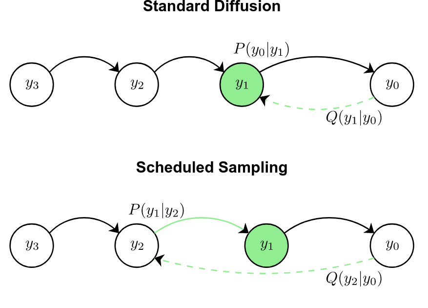
Figure 3: Diffusion samples $y_{1}$ from $Q$. Scheduled sampling instead samples an upstream latent variable $y_{2}$ and then $y_{1}$ based on the model’s Markov chain $P(y_{1}|y_{2})$.

Note that when $m=0$, ${\tilde{P}}(y_{t}|y_{0})=Q(y_{t}|y_{0})$ and we recover normal diffusion training. When $m=T-t$, ${\tilde{P}}(y_{t}|y_{0})=P(y_{t})$ if $Q(y_{T}|y_{0})=\mathcal{N}(0,I)$. An example of $m=1$ is shown in Figure 3. Substituting back, the objective becomes

$$\sum_{t=1}^{T}\mathbb{E}_{y_{t}\sim{\tilde{P}(y_{t}|y_{0})}}\left\|\frac{y_{t}-\sqrt{\bar{\alpha}_{t}}y_{0}}{\sqrt{1-\bar{\alpha}_{t}}}-\epsilon_{\theta}(y_{t},t)\right\|^{2}.$$ (3)

To compute its gradients, in theory we need to back-propagate through $\tilde{P}$ since it depends on $\theta$, but in practice to save memory we ignore $\frac{\partial\tilde{P}}{\partial\theta}$ and only consider the term inside expectation.

4 Markup-to-Image Setup

4.1 Data

We adapt datasets from four domains to the task of markup-to-image. Table 1 provides a summary of dataset statistics.

Math

Our first dataset, LaTeX-to-Math, is a large collection of real-world mathematical expressions written in LaTeX markups and their rendered images. We adopt im2latex-100k introduced in Deng et al. (2016), which is collected from Physics papers on arXiv. im2latex-100k is originally created for the visual markup decompiling task, but we adapt this dataset for the reverse task of markup-to-image. We pad all images to size $64\times 320$ and remove images larger than that size. For faster evaluation, we form a smaller test set by subsampling 1,024 examples from the original test set in im2latex-100k .

Table Layouts

The second dataset we use is based on the 100k synthesized HTML snippets and corresponding rendered webpage images from Deng et al. (2016). Each HTML snippet contains a nested $<$div$>$ with a solid border, a random width, and a random float. The maximum depth of a nest is limited to two. We make no change to this dataset, except that we subsample 1,024 examples from the original test set to form a new test set.

Sheet Music

We generate a third dataset of sheet music. The markup language LilyPond is a file format for music engraving (Nienhuys & Nieuwenhuizen, 2003). LilyPond is a powerful language for writing music scores: it allows specifying notes using letters and note durations using numbers. One challenge in the LilyPond-to-Sheet music task is to deal with the possible “relative” mode, where the determination of each note relies on where the previous note is. We generate 35k synthetic LilyPond files and compile them into sheet music. We downsample images by a factor of two and then filter out images greater than $192\times 448$.

Molecules

The last dataset we use is from the chemistry domain. The input is a string of Simplified Molecular Input Line Entry System (SMILES) which specifies atoms and bonds of a molecule (Weininger, 1988). The output is a scheme of the input molecule. We use a solubility dataset by Wilkinson et al. (2022), containing 19,925 SMILES strings. The dataset is originally proposed to improve the accessibility of chemical structures for deep learning research. 2D molecules images are rendered from SMILES strings using the Python package RDKIT (Landrum et al., 2016). We partition the data into training, validation, and test sets. We downsample images by a factor of two.

Dataset	Input Format	Input Length	# Train	# Val	# Test	Image Size	Grayscale
Math	LaTeX Math	$113$	55,033	6,072	1,024	$64\times 320$	Y
Table Layouts	HTML Snippet	481	80,000	10,000	1,024	$64\times 64$	Y
Sheet Music	LilyPond File	240	30,902	989	988	$192\times 448$	Y
Molecules	SMILES String	30	17,925	1,000	1,000	$128\times 128$	N

Table 1: Markup-to-image datasets. Inputs to each dataset are described in Section 4.1 in detail. Input length is measured as the median number of characters in the validation set.

4.2 Evaluation

Popular metrics for conditional image generation such as Inception Score (Salimans et al., 2016) or Fréchet Inception Distance (Heusel et al., 2017) evaluate the fidelity and high-level semantics of generated images. In markup-to-image tasks, we instead emphasize the pixel-level similarity between generated and ground truth images because input markups describe exactly what the image should look like.

Pixel Metrics

Our primary evaluation metric is Dynamic Time Warping (DTW) (Müller, 2007), which calculates the pixel-level similarities of images by treating them as a column time-series. We preprocess images by binarizing them. We treat binarized images as time-series by viewing each image as a sequence of column feature vectors. We evaluate the similarity of generated and ground truth images by calculating the cost of alignment between the two time-series using DTW. We use Euclidean distance as a feature matching metric. We allow minor perturbations of generated images by allowing up to 10% of upward/downward movement during feature matching.

Our secondary evaluation metric is the root squared mean error (RMSE) of pixels between generated and ground truth images. We convert all images to grayscale before calculating RMSE. While RMSE compares two images at the pixel level, one drawback is that RMSE heavily penalizes the score of symbolically equivalent images with minor perturbations.

Complimentary Metrics

Complementary to the above two main metrics, we report one learned and six classical image similarity metrics. We use CLIP score (Radford et al., 2021) as a learned metric to calculate the similarity between the CLIP embeddings of generated and ground truth images. While CLIP score is robust to minor perturbations of images, it is unclear if CLIP embeddings capture the symbolic meanings of the images in the domains of rendered markups. For classical image similarity metrics, we report SSIM (Wang et al., 2004), PSNR (Wang et al., 2004), UQI (Wang & Bovik, 2002), ERGAS (Wald, 2000), SCC (Zhou et al., 1998), and RASE (González-Audícana et al., 2004).

4.3 Experimental Setup

Model

For Math, Table Layouts, and Sheet Music datasets, we use GPT-Neo-175M (Black et al., 2021; Gao et al., 2020) as the input encoder, which incorporates source code in its pre-training. For the Molecules dataset, we use ChemBERTa-77M-MLM from DeepChem (Ramsundar et al., 2019; Chithrananda et al., 2020) to encode the input. To parameterize the diffusion decoder, we experiment with three variants of U-Net (Ronneberger et al., 2015): 1) a standard U-Net conditioned on an average-pooled encoder embedding (denoted as “-Attn,-Pos”), 2) a U-Net alternating with cross-attention layers over the full resolution of the encoder embeddings (denoted as “+Attn,-Pos”), and 3) a U-Net with both cross-attention and additional position embeddings on the query marking row ids and column ids (denoted as “+Attn,+Pos”) (Vaswani et al., 2017).

Hyperparameters

We train all models for 100 epochs using the AdamW optimizer (Kingma & Ba, 2014; Loshchilov & Hutter, 2018). The learning rate is set to $1e-4$ with a cosine decay schedule over 100 epochs and 500 warmup steps. We use a batch size of 16 for all models. For scheduled sampling, we use $m=1$. We linearly increase the rate of applying scheduled sampling from 0% to 50% from the beginning of the training to the end.

Implementation Details

Our code is built on top of the HuggingFace diffusers library. We use a single Nvidia A100 GPU to train on the Math, Table Layouts, and Molecules datasets; We use four A100s to train on the Sheet Music dataset. Training takes approximately 25 minutes per epoch for Math and Table Layouts, 30 minutes for Sheet Music, and 15 minutes for Molecules. Although one potential concern is that the scheduled sampling approach needs more compute due to the extra computation to get ${\tilde{P}}$ for $m>0$, in practice, we find that the training speed is not much affected: on the Math dataset, scheduled sampling takes 24 minutes 59 seconds per training epoch, whereas without scheduled sampling it takes 24 minutes 13 seconds per epoch.

5 Results

Approach	Pixel		Complimentary
	DTW$\downarrow$	RMSE$\downarrow$	CLIP$\uparrow$	SSIM$\uparrow$	PSNR$\uparrow$	UQI$\uparrow$	ERGAS$\downarrow$	SCC$\uparrow$	RASE$\downarrow$
Math
-Attn,-Pos	27.73	44.72	0.95	0.70	15.35	0.97	2916.76	0.02	729.19
+Attn,-Pos	20.81	39.53	0.96	0.76	16.62	0.98	2448.35	0.06	612.09
+Attn,+Pos	19.45	37.81	0.97	0.78	17.12	0.98	2314.31	0.07	578.58
Scheduled Sampling	18.81	37.19	0.97	0.79	17.25	0.98	2247.41	0.07	561.85
Table Layouts
+Attn,-Pos	6.09	22.89	0.95	0.92	38.55	0.98	2497.51	0.44	624.38
+Attn,+Pos	5.91	22.17	0.95	0.93	38.91	0.98	2409.28	0.44	602.32
Scheduled Sampling	5.64	21.11	0.95	0.93	40.20	0.98	2285.83	0.45	571.46
Sheet Music
+Attn,-Pos	81.21	45.23	0.97	0.67	15.10	0.97	3056.72	0.02	764.18
+Attn,+Pos	80.63	45.16	0.97	0.68	15.11	0.97	3032.40	0.02	758.10
Scheduled Sampling	79.76	44.70	0.97	0.68	15.20	0.97	2978.36	0.02	744.59
Molecules
+Attn,-Pos	24.87	38.12	0.97	0.61	16.66	0.98	2482.08	0.00	620.52
+Attn,+Pos	24.95	38.15	0.96	0.61	16.64	0.98	2455.18	0.00	613.79
Scheduled Sampling	24.80	37.92	0.96	0.61	16.69	0.98	2467.16	0.00	616.79

Table 2: Evaluation results of markup-to-image generation across four datasets. (+/-)Attn indicates a model with or without attention, and (+/-)Pos is a model with or without positional embeddings. Scheduled Sampling is applied to training of models with attention and positional embeddings.

Table 2 summarizes the results of markup-to-image tasks across four domains. We use DTW and RMSE as our primary evaluation metrics to make our experimental conclusions. First, we train and evaluate the variations of diffusion models on the Math dataset. Comparing the model with attention (“-Attn,-Pos”) to without attention (“+Attn,-Pos”), using attention in the model results in a significant improvement by reducing DTW (25$\%$ reduction) and RMSE (12$\%$ reduction). Therefore, we always use attention for experiments on other datasets. We observe that additionally, using positional embeddings (“+Attn,+Pos”) is helpful for the Math dataset. The proposed scheduled sampling approach improves the model’s performance using attention and positional embeddings.

We observe a similar trend in the other three datasets–Table Layouts, Sheet Music, and Molecules. Using positional embeddings improves the performance measured by DTW and RMSE (except for the Molecules dataset). Training models with the proposed scheduled sampling achieves the best results consistently across all the datasets. As noted in Figure 2, we can qualitatively observe that schedule sampling, which exposes the model to its own generations during training time, comes with the benefits of the model being capable of correcting its own mistakes at inference time.

Absolute Evaluation

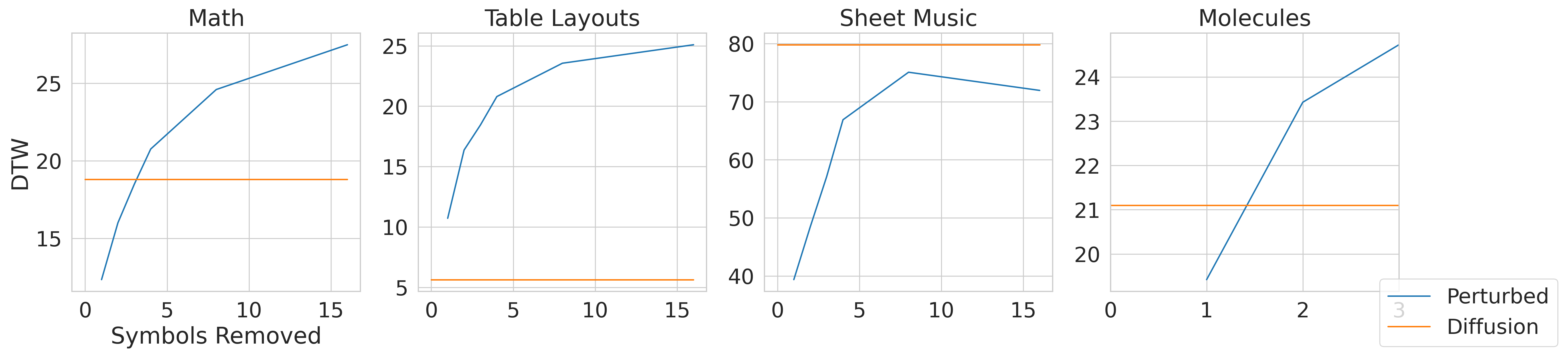
Figure 4: Perturbation results.

Our evaluation metrics enable relative comparisons between models in the markup-to-image task. However, it remains unclear how capable the models are in an absolute sense–if the models are generating near-perfect images or even the best model is missing a lot of symbols. We investigate this question by removing an increasing number of symbols from the ground truth markups and evaluating the perturbed images against the ground truth images. Our results in Figure 4 highlight that our best model performs roughly equivalent to the ground truth images with three symbols removed on the Math dataset. On the other hand, our best model performs better than ground truth images with only a single symbol removed on the Table Layouts dataset and two symbols removed on the Molecules dataset, indicating that our best model adapts to these datasets well. Results for music are less strong.

Qualitative Analysis

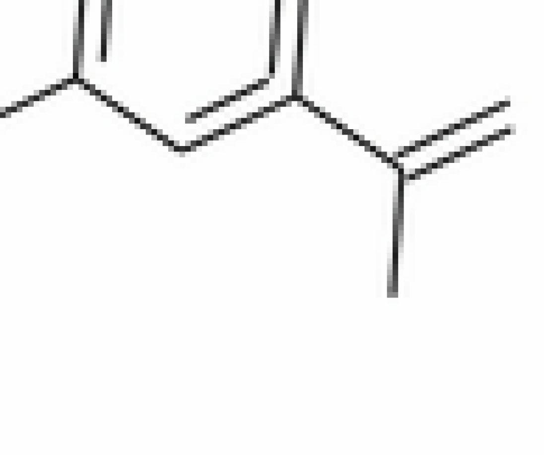
Figure 5: Qualitative results showing typical mistakes. (Top row) Model-generated images across datasets. (Bottom row) Ground truth images.

We perform qualitative analysis on the results of our best models, and we observe that diffusion models show a different level of adaptation to four datasets. First, we observe that diffusion models fully learn the Table Layouts dataset, where the majority of generated images are equivalent to the ground truth images for human eyes. Second, diffusion models perform moderately well on the Math and Molecules datasets: diffusion models generate images similar to the ground truth images most of the time on the Math dataset, but less frequently so on the Molecules dataset. The common failure modes such as dropping a few symbols, adding extra symbols, and repeating symbols are illustrated in Figure 5.

On the Sheet Music dataset, diffusion models struggle by generating images that deviate significantly from the ground truth images. Despite this, we observe that diffusion models manage to generate the first few symbols correctly in most cases. The intrinsic difficulty of the Sheet Music dataset is a long chain of dependency of symbols from left to right, and the limited number of denoising steps might be a bottleneck to generating images containing this long chain.

We provide additional qualitative results for all four datasets in Appendix A.

6 Related Work

Text-to-Image Generation

Text-to-image generation has been broadly studied in the machine learning literature, and several model families have been adopted to approach the task. Generative Adversarial Networks (Goodfellow et al., 2014) is one of the popular choices to generate realistic images from text prompts. Initiating from the pioneering work of text-to-image generation in the bird and flower domains by Reed et al. (2016a), researchers have developed methods to improve the quality of text-to-image generation via progressive refinement (Zhang et al., 2017; 2018; Zhu et al., 2019; Tao et al., 2020), cross-modal attention mechanisms (Xu et al., 2018; Zhang et al., 2021), as well as spatial and semantic modeling of objects (Koh et al., 2021; Reed et al., 2016b; Hong et al., 2018; Hinz et al., 2019). Another common method is based on VQ-VAE (Van Den Oord et al., 2017). In this approach, text-to-image generation is treated as a sequence-to-sequence task of predicting discretized image tokens autoregressively from text prompts (Ramesh et al., 2021; Ding et al., 2021; Gafni et al., 2022; Gu et al., 2022; Aghajanyan et al., 2022; Yu et al., 2022).

Diffusion models (Sohl-Dickstein et al., 2015) are the most recent progress in text-to-image generation. The simplicity of training diffusion models introduces significant utility, which often reduces to the minimization of mean-squared error for estimating noises added to images (Ho et al., 2020). Diffusion models are free from training instability or model collapses (Brock et al., 2018; Dhariwal & Nichol, 2021), and yet manage to outperform Generative Adversarial Networks on text-to-image generation in the MSCOCO domain (Dhariwal & Nichol, 2021). Diffusion models trained on large-scale image-text pairs demonstrate impressive performance in generating creative natural or artistic images (Nichol et al., 2021; Ramesh et al., 2022; Saharia et al., 2022).

So far, the demonstration of successful text-to-image generation models is centered around the scenario with flexible interpretations of text prompts (e.g., artistic image generation). When there is an exact interpretation of the given text prompt (e.g., markup-to-image generation), text-to-image generation models are understudied (with a few exceptions such as Liu et al. (2021) which studied controlled text-to-image generation in CLEVR (Johnson et al., 2017) and iGibson (Shen et al., 2021) domains). Prior work reports that state-of-the-art diffusion models face challenges in the exact interpretation scenario. For example, Ramesh et al. (2022) report unCLIP struggles to generate coherent texts based on images. In this work, we propose a controlled compositional testbed for the exact interpretation scenario across four domains. Our study brings potential opportunities for evaluating the ability of generation models to produce coherent outputs in a structured environment, and highlights open challenges of deploying diffusion models in the exact interpretation scenario.

Scheduled Sampling

In sequential prediction tasks, the mismatch between teacher forcing training and inference is known as an exposure bias or covariate shift problem (Ranzato et al., 2015; Spencer et al., 2021). During teacher forcing training, a model’s next-step prediction is based on previous steps from the ground truth sequence. During inference, the model performs the next step based on its own previous predictions. Training algorithms such as DAgger (Ross et al., 2011) or scheduled sampling (Bengio et al., 2015) are developed to mitigate this mismatch problem, primarily by forcing the model to use its own previous predictions during training with some probability. In this work, we observe a problem similar to exposure bias in diffusion models, and we demonstrate that training diffusion models using scheduled sampling improves their performance on markup-to-image generation.

7 Conclusion

We propose the task of markup-to-image generation which differs from natural image generation tasks in that there are ground truth images and deterministic compositionality. We adapt four instances of this task and show that they can be used to analyze state-of-the-art diffusion-based image generation models. Motivated by the observation that a diffusion model cannot correct its own mistakes at inference time, we propose to use scheduled sampling to expose it to its own generations during training. Experiments confirm the effectiveness of the proposed approach. The generated images are surprisingly good, but model generations are not yet robust enough for perfect rendering. We see rendering markup as an interesting benchmark and potential application of pretrained models plus diffusion.

Acknowledgments

YD is supported by an Nvidia Fellowship. NK is supported by a Masason Fellowship. AR is supported by NSF CAREER 2037519, NSF 1704834, and a Sloan Fellowship. Thanks to Bing Yan for preparing molecule data and Ge Gao for editing drafts of this paper. We would also like to thank Harvard University FAS Research Computing for providing computational resources.

Appendix A Qualitative Results

We provide additional qualitative results from models trained with or without scheduled sampling on four datasets in Figure 6, Figure 7, Figure 8, and Figure 9.

Figure 6: Qualitative results in the Math domain. Left column: ground truth images. Middle column: generations from +Attn,+Pos. Right column: generations from Scheduled Sampling. The top two rows are random selections, and the bottom two rows are examples of good generations.

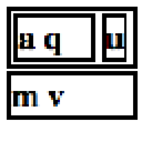
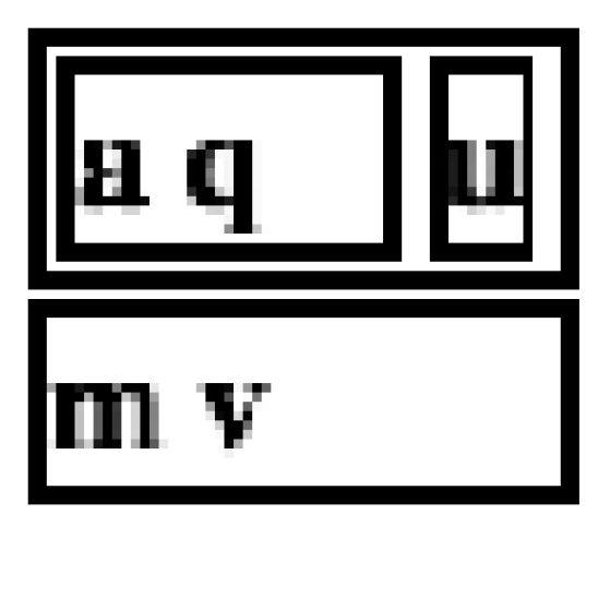
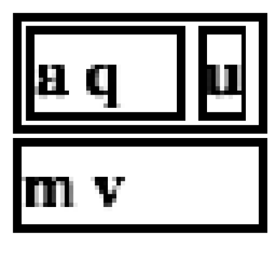
Figure 7: Qualitative results in the Table Layouts domain. Left column: ground truth images. Middle column: generations from +Attn,+Pos. Right column: generations from Scheduled Sampling. The top two rows are random selections, and the bottom two rows are examples of good generations.

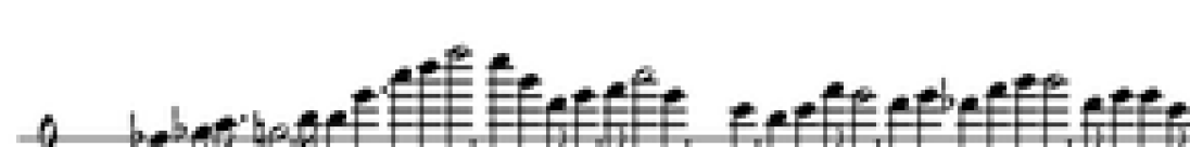
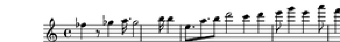
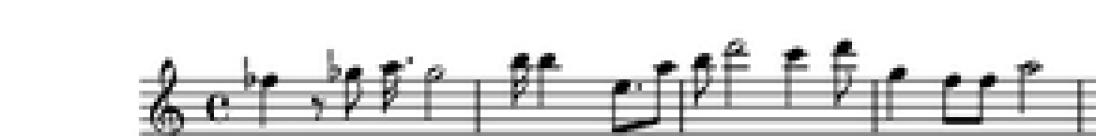
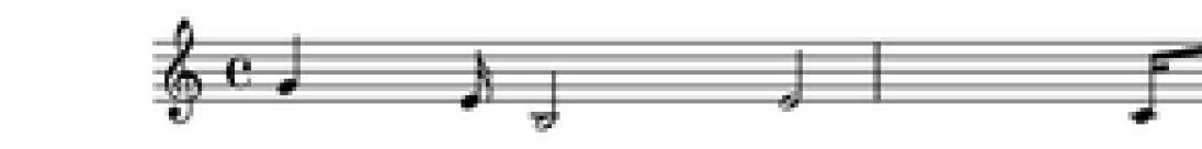
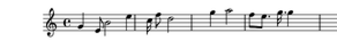
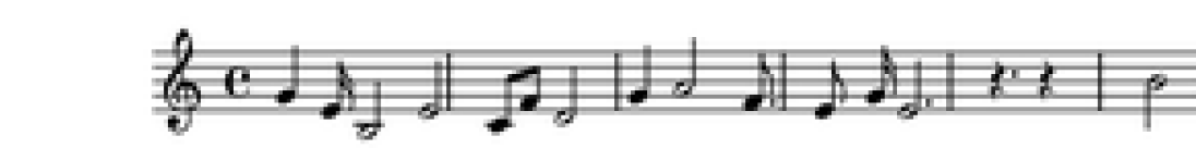
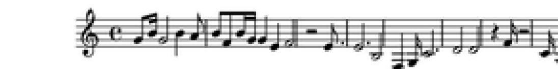
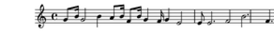
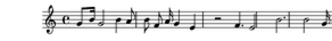
Figure 8: Qualitative results in the Sheet Music domain. Left column: ground truth images. Middle column: generations from +Attn,+Pos. Right column: generations from Scheduled Sampling. The top two rows are random selections, and the bottom two rows are examples of good generations.

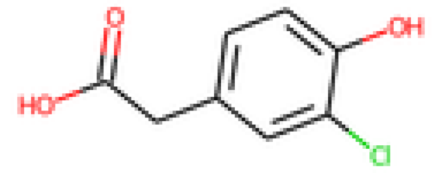
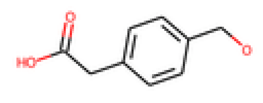
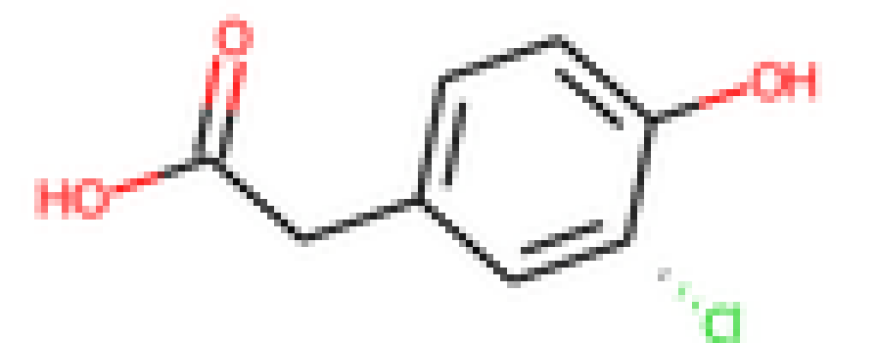
Figure 9: Qualitative results in the Molecules domain. Left column: ground truth images. Middle column: generations from +Attn,+Pos. Right column: generations from Scheduled Sampling. The top two rows are random selections, and the bottom two rows are examples of good generations.

References

- Aghajanyan et al. (2022) Armen Aghajanyan, Bernie Huang, Candace Ross, Vladimir Karpukhin, Hu Xu, Naman Goyal, Dmytro Okhonko, Mandar Joshi, Gargi Ghosh, Mike Lewis, et al. Cm3: A causal masked multimodal model of the internet. arXiv preprint arXiv:2201.07520, 2022.
- Bengio et al. (2015) Samy Bengio, Oriol Vinyals, Navdeep Jaitly, and Noam Shazeer. Scheduled sampling for sequence prediction with recurrent neural networks. Advances in neural information processing systems, 28, 2015.
- Black et al. (2021) Sid Black, Leo Gao, Phil Wang, Connor Leahy, and Stella Biderman. GPT-Neo: Large Scale Autoregressive Language Modeling with Mesh-Tensorflow, March 2021. URL https://doi.org/10.5281/zenodo.5297715.
- Brock et al. (2018) Andrew Brock, Jeff Donahue, and Karen Simonyan. Large scale gan training for high fidelity natural image synthesis. arXiv preprint arXiv:1809.11096, 2018.
- Chithrananda et al. (2020) Seyone Chithrananda, Gabriel Grand, and Bharath Ramsundar. Chemberta: large-scale self-supervised pretraining for molecular property prediction. arXiv preprint arXiv:2010.09885, 2020.
- Deng et al. (2016) Yuntian Deng, Anssi Kanervisto, and Alexander M Rush. What you get is what you see: A visual markup decompiler. arXiv preprint arXiv:1609.04938, 10:32–37, 2016.
- Dhariwal & Nichol (2021) Prafulla Dhariwal and Alexander Nichol. Diffusion models beat gans on image synthesis. Advances in Neural Information Processing Systems, 34:8780–8794, 2021.
- Ding et al. (2021) Ming Ding, Zhuoyi Yang, Wenyi Hong, Wendi Zheng, Chang Zhou, Da Yin, Junyang Lin, Xu Zou, Zhou Shao, Hongxia Yang, et al. Cogview: Mastering text-to-image generation via transformers. Advances in Neural Information Processing Systems, 34:19822–19835, 2021.
- Gafni et al. (2022) Oran Gafni, Adam Polyak, Oron Ashual, Shelly Sheynin, Devi Parikh, and Yaniv Taigman. Make-a-scene: Scene-based text-to-image generation with human priors. arXiv preprint arXiv:2203.13131, 2022.
- Gao et al. (2020) Leo Gao, Stella Biderman, Sid Black, Laurence Golding, Travis Hoppe, Charles Foster, Jason Phang, Horace He, Anish Thite, Noa Nabeshima, et al. The pile: An 800gb dataset of diverse text for language modeling. arXiv preprint arXiv:2101.00027, 2020.
- Glennie (1960) AE Glennie. On the syntax machine and the construction of a universal compiler. Technical report, CARNEGIE INST OF TECH PITTSBURGH PA COMPUTATION CENTER, 1960.
- González-Audícana et al. (2004) María González-Audícana, José Luis Saleta, Raquel García Catalán, and Rafael García. Fusion of multispectral and panchromatic images using improved ihs and pca mergers based on wavelet decomposition. IEEE Transactions on Geoscience and Remote sensing, 42(6):1291–1299, 2004.
- Goodfellow et al. (2014) Ian J Goodfellow, Jean Pouget-Abadie, Mehdi Mirza, Bing Xu, David Warde-Farley, Sherjil Ozair, Aaron C Courville, and Yoshua Bengio. Generative adversarial nets. In NIPS, 2014.
- Gu et al. (2018) Jiatao Gu, James Bradbury, Caiming Xiong, Victor OK Li, and Richard Socher. Non-autoregressive neural machine translation. In International Conference on Learning Representations, 2018.
- Gu et al. (2022) Shuyang Gu, Dong Chen, Jianmin Bao, Fang Wen, Bo Zhang, Dongdong Chen, Lu Yuan, and Baining Guo. Vector quantized diffusion model for text-to-image synthesis. In Proceedings of the IEEE/CVF Conference on Computer Vision and Pattern Recognition, pp. 10696–10706, 2022.
- Heusel et al. (2017) Martin Heusel, Hubert Ramsauer, Thomas Unterthiner, Bernhard Nessler, and Sepp Hochreiter. Gans trained by a two time-scale update rule converge to a local nash equilibrium. Advances in neural information processing systems, 30, 2017.
- Hinz et al. (2019) Tobias Hinz, Stefan Heinrich, and Stefan Wermter. Generating multiple objects at spatially distinct locations. arXiv preprint arXiv:1901.00686, 2019.
- Ho et al. (2020) Jonathan Ho, Ajay Jain, and Pieter Abbeel. Denoising diffusion probabilistic models. Advances in Neural Information Processing Systems, 33:6840–6851, 2020.
- Hong et al. (2018) Seunghoon Hong, Dingdong Yang, Jongwook Choi, and Honglak Lee. Inferring semantic layout for hierarchical text-to-image synthesis. In Proceedings of the IEEE conference on computer vision and pattern recognition, pp. 7986–7994, 2018.
- Johnson et al. (2017) Justin Johnson, Bharath Hariharan, Laurens Van Der Maaten, Li Fei-Fei, C Lawrence Zitnick, and Ross Girshick. Clevr: A diagnostic dataset for compositional language and elementary visual reasoning. In Proceedings of the IEEE conference on computer vision and pattern recognition, pp. 2901–2910, 2017.
- Kingma & Ba (2014) Diederik P Kingma and Jimmy Ba. Adam: A method for stochastic optimization. arXiv preprint arXiv:1412.6980, 2014.
- Kingma & Welling (2013) Diederik P Kingma and Max Welling. Auto-encoding variational bayes. arXiv preprint arXiv:1312.6114, 2013.
- Koh et al. (2021) Jing Yu Koh, Jason Baldridge, Honglak Lee, and Yinfei Yang. Text-to-image generation grounded by fine-grained user attention. In Proceedings of the IEEE/CVF Winter Conference on Applications of Computer Vision, pp. 237–246, 2021.
- Landrum et al. (2016) Greg Landrum et al. Rdkit: Open-source cheminformatics software. 2016. URL https://github.com/rdkit/rdkit/.
- Liu et al. (2021) Nan Liu, Shuang Li, Yilun Du, Josh Tenenbaum, and Antonio Torralba. Learning to compose visual relations. Advances in Neural Information Processing Systems, 34:23166–23178, 2021.
- Loshchilov & Hutter (2018) Ilya Loshchilov and Frank Hutter. Decoupled weight decay regularization. In International Conference on Learning Representations, 2018.
- Müller (2007) Meinard Müller. Dynamic time warping. Information retrieval for music and motion, pp. 69–84, 2007.
- Nichol et al. (2021) Alex Nichol, Prafulla Dhariwal, Aditya Ramesh, Pranav Shyam, Pamela Mishkin, Bob McGrew, Ilya Sutskever, and Mark Chen. Glide: Towards photorealistic image generation and editing with text-guided diffusion models. arXiv preprint arXiv:2112.10741, 2021.
- Nienhuys & Nieuwenhuizen (2003) Han-Wen Nienhuys and Jan Nieuwenhuizen. Lilypond, a system for automated music engraving. In Proceedings of the XIV Colloquium on Musical Informatics (XIV CIM 2003), volume 1, pp. 167–171. Citeseer, 2003.
- Radford et al. (2021) Alec Radford, Jong Wook Kim, Chris Hallacy, Aditya Ramesh, Gabriel Goh, Sandhini Agarwal, Girish Sastry, Amanda Askell, Pamela Mishkin, Jack Clark, et al. Learning transferable visual models from natural language supervision. In International Conference on Machine Learning, pp. 8748–8763. PMLR, 2021.
- Raffel et al. (2020) Colin Raffel, Noam Shazeer, Adam Roberts, Katherine Lee, Sharan Narang, Michael Matena, Yanqi Zhou, Wei Li, Peter J Liu, et al. Exploring the limits of transfer learning with a unified text-to-text transformer. J. Mach. Learn. Res., 21(140):1–67, 2020.
- Ramesh et al. (2021) Aditya Ramesh, Mikhail Pavlov, Gabriel Goh, Scott Gray, Chelsea Voss, Alec Radford, Mark Chen, and Ilya Sutskever. Zero-shot text-to-image generation. In International Conference on Machine Learning, pp. 8821–8831. PMLR, 2021.
- Ramesh et al. (2022) Aditya Ramesh, Prafulla Dhariwal, Alex Nichol, Casey Chu, and Mark Chen. Hierarchical text-conditional image generation with clip latents. arXiv preprint arXiv:2204.06125, 2022.
- Ramsundar et al. (2019) Bharath Ramsundar, Peter Eastman, Patrick Walters, Vijay Pande, Karl Leswing, and Zhenqin Wu. Deep Learning for the Life Sciences. O’Reilly Media, 2019.
- Ranzato et al. (2015) Marc’Aurelio Ranzato, Sumit Chopra, Michael Auli, and Wojciech Zaremba. Sequence level training with recurrent neural networks. arXiv preprint arXiv:1511.06732, 2015.
- Reed et al. (2016a) Scott Reed, Zeynep Akata, Xinchen Yan, Lajanugen Logeswaran, Bernt Schiele, and Honglak Lee. Generative adversarial text to image synthesis. In International conference on machine learning, pp. 1060–1069. PMLR, 2016a.
- Reed et al. (2016b) Scott E Reed, Zeynep Akata, Santosh Mohan, Samuel Tenka, Bernt Schiele, and Honglak Lee. Learning what and where to draw. Advances in neural information processing systems, 29, 2016b.
- Ronneberger et al. (2015) Olaf Ronneberger, Philipp Fischer, and Thomas Brox. U-net: Convolutional networks for biomedical image segmentation. In International Conference on Medical image computing and computer-assisted intervention, pp. 234–241. Springer, 2015.
- Ross et al. (2011) Stéphane Ross, Geoffrey Gordon, and Drew Bagnell. A reduction of imitation learning and structured prediction to no-regret online learning. In Proceedings of the fourteenth international conference on artificial intelligence and statistics, pp. 627–635. JMLR Workshop and Conference Proceedings, 2011.
- Saharia et al. (2022) Chitwan Saharia, William Chan, Saurabh Saxena, Lala Li, Jay Whang, Emily Denton, Seyed Kamyar Seyed Ghasemipour, Burcu Karagol Ayan, S Sara Mahdavi, Rapha Gontijo Lopes, et al. Photorealistic text-to-image diffusion models with deep language understanding. arXiv preprint arXiv:2205.11487, 2022.
- Salimans et al. (2016) Tim Salimans, Ian Goodfellow, Wojciech Zaremba, Vicki Cheung, Alec Radford, and Xi Chen. Improved techniques for training gans. Advances in neural information processing systems, 29, 2016.
- Shen et al. (2021) Bokui Shen, Fei Xia, Chengshu Li, Roberto Martín-Martín, Linxi Fan, Guanzhi Wang, Claudia Pérez-D’Arpino, Shyamal Buch, Sanjana Srivastava, Lyne Tchapmi, et al. igibson 1.0: a simulation environment for interactive tasks in large realistic scenes. In 2021 IEEE/RSJ International Conference on Intelligent Robots and Systems (IROS), pp. 7520–7527. IEEE, 2021.
- Sohl-Dickstein et al. (2015) Jascha Sohl-Dickstein, Eric Weiss, Niru Maheswaranathan, and Surya Ganguli. Deep unsupervised learning using nonequilibrium thermodynamics. In International Conference on Machine Learning, pp. 2256–2265. PMLR, 2015.
- Spencer et al. (2021) Jonathan Spencer, Sanjiban Choudhury, Arun Venkatraman, Brian Ziebart, and J Andrew Bagnell. Feedback in imitation learning: The three regimes of covariate shift. arXiv preprint arXiv:2102.02872, 2021.
- Tao et al. (2020) Ming Tao, Hao Tang, Songsong Wu, Nicu Sebe, Xiao-Yuan Jing, Fei Wu, and Bingkun Bao. Df-gan: Deep fusion generative adversarial networks for text-to-image synthesis. arXiv preprint arXiv:2008.05865, 2020.
- Teitelman (1972) Warren Teitelman. Automated programmering: the programmer’s assistant. In Proceedings of the December 5-7, 1972, fall joint computer conference, part II, pp. 917–921, 1972.
- Van Den Oord et al. (2017) Aaron Van Den Oord, Oriol Vinyals, et al. Neural discrete representation learning. Advances in neural information processing systems, 30, 2017.
- Vaswani et al. (2017) Ashish Vaswani, Noam Shazeer, Niki Parmar, Jakob Uszkoreit, Llion Jones, Aidan N Gomez, Łukasz Kaiser, and Illia Polosukhin. Attention is all you need. Advances in neural information processing systems, 30, 2017.
- Wald (2000) Lucien Wald. Quality of high resolution synthesised images: Is there a simple criterion? In Third conference” Fusion of Earth data: merging point measurements, raster maps and remotely sensed images”, pp. 99–103. SEE/URISCA, 2000.
- Wang & Bovik (2002) Zhou Wang and Alan C Bovik. A universal image quality index. IEEE signal processing letters, 9(3):81–84, 2002.
- Wang et al. (2004) Zhou Wang, Alan C Bovik, Hamid R Sheikh, and Eero P Simoncelli. Image quality assessment: from error visibility to structural similarity. IEEE transactions on image processing, 13(4):600–612, 2004.
- Weininger (1988) David Weininger. Smiles, a chemical language and information system. 1. introduction to methodology and encoding rules. Journal of chemical information and computer sciences, 28(1):31–36, 1988.
- Wilkinson et al. (2022) Matthew R Wilkinson, Uriel Martinez-Hernandez, Chick C Wilson, and Bernardo Castro-Dominguez. Images of chemical structures as molecular representations for deep learning. Journal of Materials Research, 37(14):2293–2303, 2022.
- Xu et al. (2018) Tao Xu, Pengchuan Zhang, Qiuyuan Huang, Han Zhang, Zhe Gan, Xiaolei Huang, and Xiaodong He. Attngan: Fine-grained text to image generation with attentional generative adversarial networks. In Proceedings of the IEEE conference on computer vision and pattern recognition, pp. 1316–1324, 2018.
- Yu et al. (2022) Jiahui Yu, Yuanzhong Xu, Jing Yu Koh, Thang Luong, Gunjan Baid, Zirui Wang, Vijay Vasudevan, Alexander Ku, Yinfei Yang, Burcu Karagol Ayan, et al. Scaling autoregressive models for content-rich text-to-image generation. arXiv preprint arXiv:2206.10789, 2022.
- Zhang et al. (2017) Han Zhang, Tao Xu, Hongsheng Li, Shaoting Zhang, Xiaogang Wang, Xiaolei Huang, and Dimitris N Metaxas. Stackgan: Text to photo-realistic image synthesis with stacked generative adversarial networks. In Proceedings of the IEEE international conference on computer vision, pp. 5907–5915, 2017.
- Zhang et al. (2018) Han Zhang, Tao Xu, Hongsheng Li, Shaoting Zhang, Xiaogang Wang, Xiaolei Huang, and Dimitris N Metaxas. Stackgan++: Realistic image synthesis with stacked generative adversarial networks. IEEE transactions on pattern analysis and machine intelligence, 41(8):1947–1962, 2018.
- Zhang et al. (2021) Han Zhang, Jing Yu Koh, Jason Baldridge, Honglak Lee, and Yinfei Yang. Cross-modal contrastive learning for text-to-image generation. In Proceedings of the IEEE/CVF conference on computer vision and pattern recognition, pp. 833–842, 2021.
- Zhou et al. (1998) Jie Zhou, Daniel L Civco, and JA Silander. A wavelet transform method to merge landsat tm and spot panchromatic data. International journal of remote sensing, 19(4):743–757, 1998.
- Zhu et al. (2019) Minfeng Zhu, Pingbo Pan, Wei Chen, and Yi Yang. Dm-gan: Dynamic memory generative adversarial networks for text-to-image synthesis. In Proceedings of the IEEE/CVF conference on computer vision and pattern recognition, pp. 5802–5810, 2019.