Mixture of Attention Heads: Selecting Attention Heads Per Token
Abstract
Mixture-of-Experts (MoE) networks have been proposed as an efficient way to scale up model capacity and implement conditional computing. However, the study of MoE components mostly focused on the feedforward layer in Transformer architecture. This paper proposes the Mixture of Attention Heads (MoA), a new architecture that combines multi-head attention with the MoE mechanism. MoA includes a set of attention heads that each has its own set of parameters. Given an input, a router dynamically selects a subset of attention heads per token. This conditional computation schema allows MoA to achieve stronger performance than the standard multi-head attention layer. Furthermore, the sparsely gated MoA can easily scale up the number of attention heads and the number of parameters while preserving computational efficiency. In addition to the performance improvements, MoA also automatically differentiates heads’ utilities, providing a new perspective to discuss the model’s interpretability. We conducted experiments on several important tasks, including Machine Translation and Masked Language Modeling. Experiments have shown promising results on several tasks against strong baselines that involve large and very deep models111The code can be found at https://github.com/yikangshen/MoA..
1 Introduction
In recent years, large models have become a popular trend in the research of Natural Language Processing, especially large-scale Transformer (Vaswani et al., 2017). The model’s capacity has increased from millions of parameters (Devlin et al., 2019; Liu et al., 2019), to billions of parameters (Shoeybi et al., 2019; Raffel et al., 2020; Wang et al., 2022), even to trillions of parameters (Du et al., 2021; Fedus et al., 2021). However, these large-scale models demand substantially more computations than small-scale models. A popular trend is to utilize conditional computation with a sparsely activated model to seek greater computational efficiency. Thus, only a part of the model’s parameters is used for a specific input during the forward computation, which alleviates the computational load.
Among these attempts, the Mixture of Experts (MoE) (Jacobs et al., 1991; Jordan and Jacobs, 1994) is an essential technique. Since first applying the mixture of experts to Transformer architecture (Shazeer et al., 2018), researchers have mainly focused on combining the Feed-Forward Network layer and the Mixture of Experts. Recent works have discussed how to get a better routing strategy (Shazeer et al., 2017; Dua et al., 2021; Lewis et al., 2021; Nie et al., 2021) or how to scale up the Mixture of Experts on different nodes of GPUs (Lepikhin et al., 2021; Fedus et al., 2021). However, few attempts have explored the possibility of combining MoE with the Multi-Head Attention (MHA) mechanism. Since the MHA is another compulsory module in the Transformer architecture, combining MoE and the attention mechanism could also help achieve better performance while restraining the computational cost.
Besides, previous research has investigated the utility of different attention heads. Peng et al. (2020) found that the combination (reallocation) of a subset of attention heads helps the Translation task since they prune the useless attention heads. In the field of dependency parsing, researchers have unveiled that some attention heads in BERT-like language models (Devlin et al., 2019; Liu et al., 2019) model individual dependency types (Htut et al., 2019) and syntactic functions (Shen et al., 2022). Voita et al. (2019) claimed that the attention heads have different functions that could be categorized into three types. There is no need to pass through all multiple attention heads for an input token if we could select some relevant attention heads whose function is proper. Thus, we conceive an attention mechanism that selects different attention heads per token.
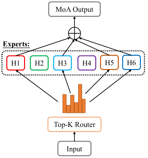
Based on the above discussion, we proposed Mixture of Attention Heads (MoA) (Section 4), an attention mechanism that selects different attention heads for different inputs. A simple illustration of this idea is shown in Figure 1. MoA includes a set of of attention heads with different parameters. Given an input, a routing network dynamically selects a subset of attention heads for each token. The output is a weighted sum of the selected attention heads given the confidence calculated by the routing network.
We conducted experiments on two tasks: Machine Translation and Masked Language Modeling (Section 5). Experiments shown promising results against several strong baselines. In all tasks, our proposed mixture of attention heads outperforms the original Transformer architecture (Vaswani et al., 2017). Our model surpasses many large models or achieves comparable results with only a half computational cost. Our contributions can be summarized in three folds: 1) We proposed a new attention mechanism called Mixture of Attention Heads, combining the idea of Mixture of Experts with the attention mechanism. 2) MoA can improve the model’s performance without substantially adding parameters and computational cost. 3) MoA is easy to scale up while maintaining with a restrained computation complexity, resulting in a further performance amelioration.
2 Related Work
Mixture of Experts
The Mixture of Experts (MoE) was firstly introduced in the 1990s (Jacobs et al., 1991; Jordan and Jacobs, 1994). Shazeer et al. (2017) adopted this method into modern deep learning architectures (LSTM; Hochreiter and Schmidhuber 1997) and proved its effectiveness in Language Modeling and Machine Translation. The MoE was used to substitute the FFN layers in Transformer architecture (Vaswani et al., 2017) by the Mesh Tensorflow library (Shazeer et al., 2018). Gshard (Lepikhin et al., 2021) is a lightweight module that helps scale up multilingual neural machine translation Transformer with a Sparsely-Gated Mixture of Experts beyond 600 billion parameters. In Switch Transformer (Fedus et al., 2021), the authors scaled the MoE-integrated Transformer architecture toward trillion parameter models. GLaM (Du et al., 2021) utilized a decoder-only architecture to do language model pre-training. Rajbhandari et al. (2022) proposed a Pyramid-Residual-MoE for smaller model size and fast inference.
Various routing strategies (Shazeer et al., 2017; Dua et al., 2021; Lewis et al., 2021; Nie et al., 2021) have been investigated for stabilizing the MoE training and balancing the expert loads. Chi et al. (2022) pointed out the representation collapse issue in the sparse Mixture of Experts models and solved by a two-stage routing strategy.
Machine Translation Architectures
With original Transformer architecture (Vaswani et al., 2017), Ott et al. (2018) found that training with reduced precision and large batch could improve the translation performance. Some models get better performance on translation by using larger scale of Transformer. Liu et al. (2020a) deepened the encoder and decoder of the Transformer by adequately initializing the model. DeepNet (Wang et al., 2022) scaled Transformers up to 1,000 layers by introducing a new normalization function. However, these methods require a great amount of computational cost. Some models make changes to the self-attention module. Peng et al. (2020) proposed MAE model. The reallocation of attention heads got better performance on Translation, since the model prune useless multi-head attention heads. However, their method is difficult to scale up and get further improvement of the results because it needs to use all the attention heads in the model rather than sparsely activate them. It also requires the complicated block coordinate descent training steps. Wu et al. (2019) proposed DynamicConv and LightConv by replacing self-attention mechanism with a lightweight convolution.
Specialization of Attention Heads
Since the publication of Transformer architecture (Vaswani et al., 2017), many researchers have been interested in analyzing how the attention mechanism works. Voita et al. (2019) systematically analyzed the attention heads in the encoder and categorized them into three functional subsets: positional, syntactic, and rare words. When dealing with dependency parsing, researchers also observed the same phenomenon that different heads could capture different syntactic functions (Htut et al., 2019; Shen et al., 2022).
3 Preliminaries
3.1 Mixture of Experts
MoE (Shazeer et al., 2017) contains a set of expert networks and a routing network . The output of the MoE is the weighted sum of the output of each expert. The routing network calculates the probability for each expert. Formally, the output of the MoE can be written as:
| (1) |
3.2 Multi-head Attention
Vaswani et al. (2017) proposed an encoder-decoder architecture Transformer, which contains the multi-head attention module. Different heads from the multi-head attention module attend to information from different representation subspaces, which learn the input from various perspectives.
Performing multi-head attention with heads, the are linearly projected times with different, learned linear projections to subspaces. On each projected and , the attention scores are calculated, via Equation 4. Values deriving from different heads are projected back to the model dimension size and summed up, with Equation 5.
| (4) |
| (5) |
where and , is the dimension of the key .
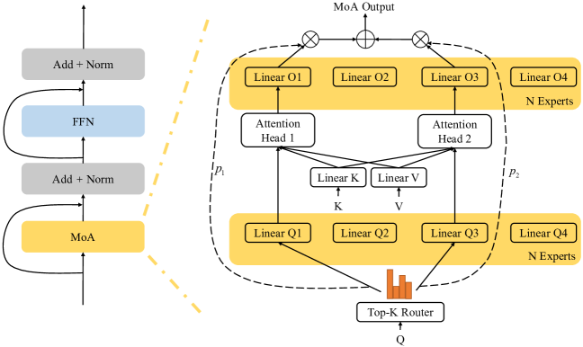
4 Mixture of Attention Heads
In this work, we propose a variant of multi-head attention for Transformer called Mixture of Attention Heads (MoA), illustrated in Figure 2. MoA consists of two major components, the routing network and a group of attention experts . Similar to standard multi-head self-attention, the input of MoA includes three sequences, query sequence , key sequence , and value sequence . We note as the query vector at time step . For each , the routing network selects a subset of experts based on and assign a weight to each selected expert. Then, these selected experts take , , and as inputs and compute an output . The output of the MoA is the weighted sum of the selected experts’ outputs. Formally, the MoA output at time step can be written as:
| (6) |
4.1 Routing Network
Similar to previous mixture-of-expert methods, the routing network assigns attention experts to input query. In order to select experts for query , we compute a routing probability for each expert . The routing probability is modeled with a linear layer and a softmax function:
| (7) |
Based on the routing probability , we select the top- attention experts among all attention experts with the largest probabilities. Formally, the routing network is defined as:
| (8) |
where , representing the routing matrix. Then, we renormalize the routing probability of the selected experts to get normalized expert weights:
| (9) |
where is a function that stops the gradient backpropagation. In other words, the denominator receives zero gradient during the training process. We empirically find that this trick helps the routing network learn better routing probability.
4.2 Attention Expert
An attention expert contains four different projection matrices, , , and . The attention calculation is similar to multi-head attention. We first compute the attention weight for keys.
| (10) |
where is the query projection matrix, is the key projection matrix, is the hidden state size, is named as head dimension. We then compute the weighted sum of values:
| (11) |
where is the value projection matrix. Finally, the attention output is obtained by projecting back to the hidden state space:
| (12) |
where is the output projection matrix.
In the multi-head attention, the projection matrices , , , and are all different across attention heads. The MoA shares and across attention experts to reduce the computational complexity. Attention experts are only differentiated by and . Thus, the expensive matrix projection of key sequence and value sequence can be pre-computed and shared for all attention experts. Each expert only need to compute the vector projection of query and output . This design can significantly reduce the computational and space complexity while the number of experts is large.
4.3 Training Losses
Previous work (Shazeer et al., 2017) has observed that the routing network tends to converge to a state where it always produces large weights for the same few experts, which indicates the insufficient utility of all the experts. Following Shazeer et al. (2017) and Fedus et al. (2021), we add an auxiliary loss to balance the loads of different experts.
Given experts and a sequence with queries , the auxiliary loss can be computed as:
| (13) |
where is the number of tokens attributed to the -th expert,
| (14) |
where represents the Kronecker-Symbol. is the sum of router probability allocated for the -th expert,
| (15) |
They are then normalized with norm 1 according to the expert column. Mathematically, is indifferentiable while is. Thus, larger will result in a larger derivative. This penalizes the making larger smaller. What’s more, is calculated by softmax. Thus smaller will become bigger.
Zoph et al. (2022) introduced a router z-loss (Equation 16) to penalize large logits into the gating network, which could stabilize the training and improve the performance.
| (16) |
where is the pre-softmax logit computed by router for -th expert and input query . Each mixture of attention heads module has an auxiliary loss and a router z-loss. We sum them up together and added with a multiplicative coefficient and respectively to the total model loss during training. Throughout this work, we use and to ensure the efficiency of the two added losses and not to disturb the primary cross-entropy model loss.
| (17) |
To validate the utility of these auxiliary losses, we conducted ablation tests and the results are shown in Appendix D.
4.4 Computational Complexity and Number of Parameters
On the one hand, given a sequence with tokens, the amount of computation required by an MoA layer that selects top- experts is
| (18) |
where is the sum of head dimension of selected experts. It represents the maximum amount of information that can be collected by an MoA layer for a token. On the other hand, the amount of computation required by a standard Multi-Head Attention (MHA) is
| (19) |
where is the sum of head dimension. If , the computational complexity of MoA is smaller than that of MHA. In other words, the MoA could collect more information for each token while maintaining a similar level of computational complexity as the MHA.
As for the number of parameters, given a Mixture of Attention Heads with attention experts, the number of parameters in MoA and MHA are:
| (20) |
When and , the number of parameters in MoA is smaller than MHA. In other words, MoA could collect more information for each token while maintaining a similar number of parameters as MHA. More details of the calculation are in Appendix B.
The above discussion suggests that, from an information collection point of view, the MoA is more computational and parameter efficient than the standard MHA. Our experimental results in Section 5 also empirically support the hypothesis. Additionally, the time complexity of MoA is decided by the number of attention heads and the attention head dimension , not the model’s total parameters. One could arbitrarily increase the amount of parameters in MoA, without increasing its computational complexity.
5 Experiments
5.1 Machine Translation
Dataset
We train our Mixture of Attention model on WMT 2014 English-German and English-French datasets (Bojar et al., 2014). Following the experimental settings used in Liu et al. (2020b), all sentences were encoded using byte-pair encoding (Sennrich et al., 2016). For both tasks, we use a joined dictionary and share all word embeddings of the encoder and the decoder. For English-German, their shared vocabulary size is set to be 32k. For English-French, their shared vocabulary size is set to be 40k.
| Model | WMT14 EnDe | WMT14 EnFr | MACs333We adopt the open-source tool ptflops (https://github.com/sovrasov/flops-counter.pytorch) to calculate the MACs. | ||
|---|---|---|---|---|---|
| #Params | BLEU | #Params | BLEU | ||
| Transformer base (Vaswani et al., 2017) | 65M | 27.3 | 62M | 38.1 | 604M |
| Admin 6L-6L (Liu et al., 2020b) | 61M | 27.7 | 67M | 41.5 | 604M |
| MAE-7 (Peng et al., 2020) | 63M | 28.4 | - | - | - |
| MoA Base () | 65M | 28.4 | 69M | 42.5 | 628M |
| Transformer big (Vaswani et al., 2017) | 213M | 28.4 | 210M | 41.8 | 2090M |
| Transformer big (Ott et al., 2018) | 210M | 29.3 | 222M | 43.2 | 2090M |
| LightConv (Wu et al., 2019) | 202M | 28.9 | - | 43.1 | 1750M444These MACs values are underestimated. Because the ptflops does not support the customized convolution layers in DynamicConv and LightConv. |
| DynamicConv (Wu et al., 2019) | 213M | 29.7 | - | 43.2 | 1790M444These MACs values are underestimated. Because the ptflops does not support the customized convolution layers in DynamicConv and LightConv. |
| Admin 18L-18L (Liu et al., 2020b) | 151M | 29.0 | - | - | 1490M |
| Admin 60L-12L (Liu et al., 2020b) | 256M | 30.1 | 262M | 43.8 | 2550M |
| MoA Big () | 200M | 29.4 | 204M | 43.7 | 1220M |
Training and Evaluation Details
We use the Adam Optimizer (Kingma and Ba, 2015) with a learning rate of and the inverse square root learning rate scheduler. During training, we employed label smoothing (Szegedy et al., 2016) of value 0.1. More training details can be found in Appendix C.
For the evaluation, we average the last 10 epochs’ checkpoints. We list BLEU score (Papineni et al., 2002) computed with multi-bleu.perl, and apply the compound split post-processing222https://github.com/tensorflow/tensor2tensor/blob/master/tensor2tensor/utils/get_ende_bleu.sh introduced in Vaswani et al. (2017). We use MACs (Multiply–Accumulate Operations)333We adopt the open-source tool ptflops (https://github.com/sovrasov/flops-counter.pytorch) to calculate the MACs. to evaluate the computational complexity of different models on a fixed input. Details of the MACs calculation are in Appendix E.
Baselines
We compare with several strong baselines: Transformer base and big (Vaswani et al., 2017), Transformer big (Ott et al., 2018) with reduced precision and large batch training, DynamicConv (Wu et al., 2019) by replacing self-attention mechanism with a lightweight convolution, MAE-7 with reallocation of attention heads proposed by Peng et al. (2020), Admin (Liu et al., 2020a) which deepens the Transformer architecture.
For our model, three parameters are used to differentiate its variants, one is number of the activated attention heads () per token, one is total number of the experts (), another is the attention expert dimension (). For example, our MoA base model is noted as , because it has 8 attention experts, 128 dimension per expert, and all 8 experts are activated for each token. Our MoA big model is as it has 32 attention experts and sparsely activates the top 16 experts for each token.
Results
The results on the test set of WMT14 EnDe and WMT14 EnFr datasets are shown in Table 3. The table is split into 2 parts, the upper part is for base models and the lower part is for large models. On all datasets, MoA base outperforms Transformer base and Admin 6L-6L by at least 0.6 BLEU. On the WMT14 EnFr dataset, MoA base also outperforms Transformer big. On the WMT14 EnDe dataset, MoA base reaches comparable results with the Mixture of Attention Experts model (MAE-7), which is the state-of-the-art performance for base-level models. MACs of MAE-7 and our model are comparable in the setting of 8 attention heads. While both models leverage the idea of weighting the attention heads, MoA is easier to implement and does not require the complicated block coordinate descent training steps. Compared to standard multi-head self-attention, the routing mechanism pays more attention to the more informative attention heads for each token, thus enabling the MoA base model to achieve better computation and parameter efficiency.
In the big-scale setting, MoA big consistently outperforms standard transformer big models, despite requiring significantly less computation. Compared to the models with more parameters, MoA is still very competitive. Only Admin 60L-12L outperforms MoA big on both datasets. However, the model has more parameters and requires about two times of MACs. The MACs of MoA big is 1220M, which is the lowest amount among big-scale models. This result shows that our proposed method could easily scale up to a large amount of parameters and achieve good results without substantially burdening the computation system.
| Model | #Params | PPL | MACs | |
|---|---|---|---|---|
| Transformer | 51.34M | 4.95 | 6.55G | |
| MoA | 52.45M | 4.82 | 7.27G | |
| 61.89M | 4.64 | 8.97G | ||
| 78.75M | 4.48 | 8.97G | ||
| 112.47M | 4.25 | 8.98G | ||
| 179.91M | 4.21 | 8.98G | ||
| MoA Model | #Params | PPL(Valid) | BLEU(Test) | MACs | |||
|---|---|---|---|---|---|---|---|
| Base | 8 | 8 | 128 | 65M | 4.68 | 28.4 | 628M |
| (A) | 8 | 8 | 256 | 87M | 4.51 | 28.7 | 841M |
| (B) | 8 | 16 | 256 | 125M | 4.45 | 28.4 | 841M |
| (C) | 8 | 32 | 64 | 83M | 4.79 | 27.9 | 524M |
| (D) | 8 | 32 | 128 | 123M | 4.55 | 28.4 | 631M |
| (E) | 8 | 32 | 256 | 200M | 4.44 | 28.8 | 841M |
| (F) | 4 | 32 | 256 | 200M | 4.65 | 27.5 | 654M |
| Big | 16 | 32 | 256 | 200M | 4.35 | 29.4 | 1220M |
5.2 Masked Language Modeling
Masked Language Modeling is the standard training objective for many Pretrained Language Models (PLMs), including BERT (Devlin et al., 2019) and RoBERTa (Liu et al., 2019). The task replaces a random sample of tokens in the input sequence with a special token [MASK]. The training objective is a cross-entropy loss on predicting the masked tokens. To better mimic the procedure of training PLMs, we adopt the setting introduced in RoBERTa (Liu et al., 2019) to conduct the masked language modeling experiment.
Dataset
We conducted the masked language modeling on the wikitext-103 dataset (Merity et al., 2016). The corpus includes over 100 million tokens collected from verified Good and Featured articles on English Wikipedia. Following the settings in Merity et al. (2016), the training/validation/test set has 103M/218K/246K words. The corpus is tokenized with the 50K subword vocabulary used in RoBERTa and initially introduced in GPT (Radford et al., 2019).
Settings
Then we train the model with the dynamic masking strategy and full-sentences input format. To avoid overfitting on the training corpus, we adopt a medium-size RoBERTa model as the base model, with 512-dim word embedding, 2048-dim feed-forward network, 8 heads, and 8 layers. Training details can be found in Appendix C. The perplexity is used as the evaluation metric.
Results
Table 2 shows the perplexity on WikiText-103 test data. While using a similar amount of parameters, MoA outperforms the standard transformer model by 0.13 perplexity. Furthermore, the performance simultaneously improves with the increase of number of experts and head size , while the number of selected heads and the computational complexity remains the same. The observation shows that our model has the ability of increasing the model’s performance while maintaining the computation complexity.
5.3 Model Analysis
MoA parameter influence
We study the influence of three parameters, , , and , on the WMT14 En-De Dataset. The results are shown in Table 3. For the expert dimension , we control and , vary the expert dimension with 64, 128, and 256. As the expert dimension size increases (rows C, D, E in Table 3), the PPL on the validation set and the BLEU score on the test set both improve. This amelioration is due to the increase in parameters. With a larger expert dimension size, each expert has more parameters, and the computational costs increase. We believe the increase in computational cost is acceptable. As in Table 3, Transformer big model has a MACs of 2090M, reaching BLEU of 28.4. However, by enlarging hidden size of expert, we could get BLEU of 28.8 while MACs at 841M (<<2090M).
For the number of attention experts , we control and , select three different values of , 8, 16, and 32. When adding the number of experts, the PPL on the valid set goes down, indicating our model’s continuous scaling up ability. The BLEU score on the test set does not change with that of PPL, and this may be because the training objective is not directly linked to the BLEU score calculation. However, we still observe that 32 experts can achieve better BLEU than the other two settings. As the number of selected attention heads remains unchanged, the MACs for these three settings are the same. Thus, MoA allows us to improve the model ability by adding more parameters without changing the computational complexity.
For the number of selected attention heads , we test three numbers of selected attention heads , 4, 8, and 16, freezing and . With the increase in the number of selected attention heads, we observe that the PPL on the valid set decreases and the BLEU score on the test set goes up. Since the number of attention experts remains the same, the model’s total parameters stay at 200M. This result shows the trade-off between computation efficiency and performance. The model needs more computations for better performance as the MACs vary from 654M to 1220M.
MoA Expert loads
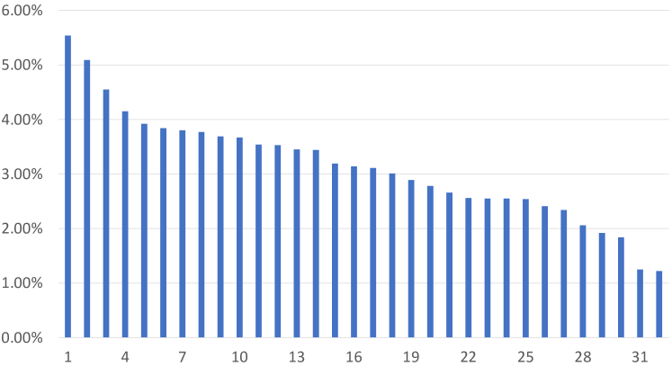
Load balancing is a long-standing problem of MoE models (Fedus et al., 2021). Figure 3 shows the experts’ load of the fourth layer of the MoA big model. It plots the percentage of each expert used in the development set of WMT14 EN-DE. For each input token and MoA big, 16 attention heads are selected among 32 attention experts. This figure shows a relatively based load, where the most used expert is selected by 5% of the tokens and the least used expert is selected by 1%, and most experts’ loads are between 2-4%. This observation suggests that the input tokens are attributed equally among attention experts. Experts are assigned to different roles with substantially different groups of input tokens. The load for every expert of different layers is shown in Appendix A.
MoA Interpretability: Specialize the Experts
| Expert 5 | Expert 29 | Expert 10 |
| Tech. | adv. | Location |
| DSL | likely | Costasur |
| JPEG | tastefully | Kaliningrad |
| Module | environmentally | Freiburg |
| DSLR | heavily | Brava |
| screen | certainly | Jesolo |
| Expert 7 | Expert 24 | Expert 23 |
| Computer | Reaction | Name |
| Outlook | supportive | Marx |
| Excel | misunderstanding | Jarzembowski |
| IO | advocating | Reding |
| emails | confirming | Donald |
| monitors | excitement | Socrates |
We study in this section whether the different experts possess different “expertises”. We try to find the most likely tokens to co-occur with each expert. We compute the pointwise mutual information (PMI; Church and Hanks 1990) between tokens and experts:
For each expert, the bigger the PMI, the more relevant the token with this expert. Table 4 lists the most indicative tokens of each expert for the first encoder layer of . Many experts are associated with nouns in the same topic, e.g., Location, Name, Tech, etc. We also found that some other experts are associated with adjectives and adverbs. For example, Expert 29 is related to adverbs, and Expert 24 is connected to people’s reactions, where some tokens are adjectives. We also study the relation between expert and input tokens for other layers of the encoder, but it is hard to find clear patterns in other layers.
6 Conclusion
This work introduces the Mixture of Attention Heads (MoA). MoA contains a set of attention experts and a routing network. Given an input, the MoA attributes a probability to each expert by the routing network and selects the top-K experts. The output of MoA is a weighted sum of the selected attention experts. The weighting mechanism allows different tokens to focus on different experts, thus improving the model’s parameter and computation efficiency. Experimental results show that a base-scale MoA model could achieve comparable or better performance than a transformer big model. Furthermore, MoA could improve its performance by adding more attention experts while maintaining a relatively small computational complexity. In this way, MoA can achieve comparable performance with deeper and computationally more expensive models. The interpretability analysis shows that different attention experts tend to specialize in a specific type of input tokens.
Limitations
In this work, we scale up MoA to at most 64 experts. However, regarding the works combining mixture of experts with FFN layer, they could expand the expert number to thousands. In the future, we will explore the limit of the scale up ability of MoA.
Our implementation of MoA is not optimistic. Our code could not fully explore the parallel computing capability of GPUs. Our current implementation spends some extra time on memory copy operations. Although the computational complexity (MACs) of MoA is relatively low compared to other baselines, the running time of our implementation is not optimal. In the future, if we could optimize the implementation at the cuda kernel level to remove the memory copy ops, we expect at least half the wall-clock time. This will make an MoA block as fast as a standard attention block.
Similar to Transformer architecture, MoA needs a careful hyperparameter search to reach satisfying results.
Acknowledgments
This work is supported in part by the State Key Laboratory of the Software Development Environment of China under Grant SKLSDE-2021ZX-16.
References
- Bojar et al. (2014) Ondrej Bojar, Christian Buck, Christian Federmann, Barry Haddow, Philipp Koehn, Johannes Leveling, Christof Monz, Pavel Pecina, Matt Post, Herve Saint-Amand, Radu Soricut, Lucia Specia, and Ales Tamchyna. 2014. Findings of the 2014 workshop on statistical machine translation. In Proceedings of the Ninth Workshop on Statistical Machine Translation, pages 12–58. The Association for Computer Linguistics.
- Chi et al. (2022) Zewen Chi, Li Dong, Shaohan Huang, Damai Dai, Shuming Ma, Barun Patra, Saksham Singhal, Payal Bajaj, Xia Song, and Furu Wei. 2022. On the representation collapse of sparse mixture of experts. CoRR, abs/2204.09179.
- Church and Hanks (1990) Kenneth Ward Church and Patrick Hanks. 1990. Word association norms, mutual information, and lexicography. Comput. Linguistics, 16(1):22–29.
- Devlin et al. (2019) Jacob Devlin, Ming-Wei Chang, Kenton Lee, and Kristina Toutanova. 2019. BERT: pre-training of deep bidirectional transformers for language understanding. In Proceedings of the 2019 Conference of the North American Chapter of the Association for Computational Linguistics: Human Language Technologies, pages 4171–4186. Association for Computational Linguistics.
- Du et al. (2021) Nan Du, Yanping Huang, Andrew M. Dai, Simon Tong, Dmitry Lepikhin, Yuanzhong Xu, Maxim Krikun, Yanqi Zhou, Adams Wei Yu, Orhan Firat, Barret Zoph, Liam Fedus, Maarten Bosma, Zongwei Zhou, Tao Wang, Yu Emma Wang, Kellie Webster, Marie Pellat, Kevin Robinson, Kathy Meier-Hellstern, Toju Duke, Lucas Dixon, Kun Zhang, Quoc V. Le, Yonghui Wu, Zhifeng Chen, and Claire Cui. 2021. Glam: Efficient scaling of language models with mixture-of-experts. CoRR, abs/2112.06905.
- Dua et al. (2021) Dheeru Dua, Shruti Bhosale, Vedanuj Goswami, James Cross, Mike Lewis, and Angela Fan. 2021. Tricks for training sparse translation models. CoRR, abs/2110.08246.
- Fedus et al. (2021) William Fedus, Barret Zoph, and Noam Shazeer. 2021. Switch transformers: Scaling to trillion parameter models with simple and efficient sparsity. CoRR, abs/2101.03961.
- Hochreiter and Schmidhuber (1997) Sepp Hochreiter and Jürgen Schmidhuber. 1997. Long short-term memory. Neural Comput., 9(8):1735–1780.
- Htut et al. (2019) Phu Mon Htut, Jason Phang, Shikha Bordia, and Samuel R. Bowman. 2019. Do attention heads in BERT track syntactic dependencies? CoRR, abs/1911.12246.
- Jacobs et al. (1991) Robert A. Jacobs, Michael I. Jordan, Steven J. Nowlan, and Geoffrey E. Hinton. 1991. Adaptive mixtures of local experts. Neural Comput., 3(1):79–87.
- Jordan and Jacobs (1994) Michael I. Jordan and Robert A. Jacobs. 1994. Hierarchical mixtures of experts and the EM algorithm. Neural Comput., 6(2):181–214.
- Kingma and Ba (2015) Diederik P. Kingma and Jimmy Ba. 2015. Adam: A method for stochastic optimization. In 3rd International Conference on Learning Representations.
- Lepikhin et al. (2021) Dmitry Lepikhin, HyoukJoong Lee, Yuanzhong Xu, Dehao Chen, Orhan Firat, Yanping Huang, Maxim Krikun, Noam Shazeer, and Zhifeng Chen. 2021. Gshard: Scaling giant models with conditional computation and automatic sharding. In 9th International Conference on Learning Representations. OpenReview.net.
- Lewis et al. (2021) Mike Lewis, Shruti Bhosale, Tim Dettmers, Naman Goyal, and Luke Zettlemoyer. 2021. BASE layers: Simplifying training of large, sparse models. In Proceedings of the 38th International Conference on Machine Learning, volume 139 of Proceedings of Machine Learning Research, pages 6265–6274. PMLR.
- Liu et al. (2020a) Liyuan Liu, Xiaodong Liu, Jianfeng Gao, Weizhu Chen, and Jiawei Han. 2020a. Understanding the difficulty of training transformers. In Proceedings of the 2020 Conference on Empirical Methods in Natural Language Processing, pages 5747–5763. Association for Computational Linguistics.
- Liu et al. (2020b) Xiaodong Liu, Kevin Duh, Liyuan Liu, and Jianfeng Gao. 2020b. Very deep transformers for neural machine translation. CoRR, abs/2008.07772.
- Liu et al. (2019) Yinhan Liu, Myle Ott, Naman Goyal, Jingfei Du, Mandar Joshi, Danqi Chen, Omer Levy, Mike Lewis, Luke Zettlemoyer, and Veselin Stoyanov. 2019. Roberta: A robustly optimized BERT pretraining approach. CoRR, abs/1907.11692.
- Merity et al. (2016) Stephen Merity, Caiming Xiong, James Bradbury, and Richard Socher. 2016. Pointer sentinel mixture models.
- Nie et al. (2021) Xiaonan Nie, Shijie Cao, Xupeng Miao, Lingxiao Ma, Jilong Xue, Youshan Miao, Zichao Yang, Zhi Yang, and Bin Cui. 2021. Dense-to-sparse gate for mixture-of-experts. CoRR, abs/2112.14397.
- Ott et al. (2018) Myle Ott, Sergey Edunov, David Grangier, and Michael Auli. 2018. Scaling neural machine translation. In Proceedings of the Third Conference on Machine Translation: Research Papers, pages 1–9, Brussels, Belgium. Association for Computational Linguistics.
- Papineni et al. (2002) Kishore Papineni, Salim Roukos, Todd Ward, and Wei-Jing Zhu. 2002. Bleu: a method for automatic evaluation of machine translation. In Proceedings of the 40th Annual Meeting of the Association for Computational Linguistics, pages 311–318. ACL.
- Peng et al. (2020) Hao Peng, Roy Schwartz, Dianqi Li, and Noah A. Smith. 2020. A mixture of h - 1 heads is better than h heads. In Proceedings of the 58th Annual Meeting of the Association for Computational Linguistics, pages 6566–6577. Association for Computational Linguistics.
- Radford et al. (2019) Alec Radford, Jeffrey Wu, Rewon Child, David Luan, Dario Amodei, Ilya Sutskever, et al. 2019. Language models are unsupervised multitask learners. OpenAI blog, 1(8):9.
- Raffel et al. (2020) Colin Raffel, Noam Shazeer, Adam Roberts, Katherine Lee, Sharan Narang, Michael Matena, Yanqi Zhou, Wei Li, and Peter J. Liu. 2020. Exploring the limits of transfer learning with a unified text-to-text transformer. J. Mach. Learn. Res., 21:140:1–140:67.
- Rajbhandari et al. (2022) Samyam Rajbhandari, Conglong Li, Zhewei Yao, Minjia Zhang, Reza Yazdani Aminabadi, Ammar Ahmad Awan, Jeff Rasley, and Yuxiong He. 2022. Deepspeed-moe: Advancing mixture-of-experts inference and training to power next-generation AI scale. CoRR, abs/2201.05596.
- Sennrich et al. (2016) Rico Sennrich, Barry Haddow, and Alexandra Birch. 2016. Neural machine translation of rare words with subword units. In Proceedings of the 54th Annual Meeting of the Association for Computational Linguistics (Volume 1: Long Papers), pages 1715–1725, Berlin, Germany. Association for Computational Linguistics.
- Shazeer et al. (2018) Noam Shazeer, Youlong Cheng, Niki Parmar, Dustin Tran, Ashish Vaswani, Penporn Koanantakool, Peter Hawkins, HyoukJoong Lee, Mingsheng Hong, Cliff Young, Ryan Sepassi, and Blake A. Hechtman. 2018. Mesh-tensorflow: Deep learning for supercomputers. In Advances in Neural Information Processing Systems 31, pages 10435–10444.
- Shazeer et al. (2017) Noam Shazeer, Azalia Mirhoseini, Krzysztof Maziarz, Andy Davis, Quoc V. Le, Geoffrey E. Hinton, and Jeff Dean. 2017. Outrageously large neural networks: The sparsely-gated mixture-of-experts layer. In 5th International Conference on Learning Representations. OpenReview.net.
- Shen et al. (2022) Yikang Shen, Shawn Tan, Alessandro Sordoni, Peng Li, Jie Zhou, and Aaron C. Courville. 2022. Unsupervised dependency graph network. In Proceedings of the 60th Annual Meeting of the Association for Computational Linguistics (Volume 1: Long Papers), pages 4767–4784. Association for Computational Linguistics.
- Shoeybi et al. (2019) Mohammad Shoeybi, Mostofa Patwary, Raul Puri, Patrick LeGresley, Jared Casper, and Bryan Catanzaro. 2019. Megatron-lm: Training multi-billion parameter language models using model parallelism. CoRR, abs/1909.08053.
- Szegedy et al. (2016) Christian Szegedy, Vincent Vanhoucke, Sergey Ioffe, Jonathon Shlens, and Zbigniew Wojna. 2016. Rethinking the inception architecture for computer vision. In 2016 IEEE Conference on Computer Vision and Pattern Recognition, pages 2818–2826. IEEE Computer Society.
- Vaswani et al. (2017) Ashish Vaswani, Noam Shazeer, Niki Parmar, Jakob Uszkoreit, Llion Jones, Aidan N. Gomez, Lukasz Kaiser, and Illia Polosukhin. 2017. Attention is all you need. In Advances in Neural Information Processing Systems 30, pages 5998–6008.
- Voita et al. (2019) Elena Voita, David Talbot, Fedor Moiseev, Rico Sennrich, and Ivan Titov. 2019. Analyzing multi-head self-attention: Specialized heads do the heavy lifting, the rest can be pruned. In Proceedings of the 57th Conference of the Association for Computational Linguistics, pages 5797–5808. Association for Computational Linguistics.
- Wang et al. (2022) Hongyu Wang, Shuming Ma, Li Dong, Shaohan Huang, Dongdong Zhang, and Furu Wei. 2022. Deepnet: Scaling transformers to 1, 000 layers. CoRR, abs/2203.00555.
- Wu et al. (2019) Felix Wu, Angela Fan, Alexei Baevski, Yann N. Dauphin, and Michael Auli. 2019. Pay less attention with lightweight and dynamic convolutions. In 7th International Conference on Learning Representations. OpenReview.net.
- Zoph et al. (2022) Barret Zoph, Irwan Bello, Sameer Kumar, Nan Du, Yanping Huang, Jeff Dean, Noam Shazeer, and William Fedus. 2022. Designing effective sparse expert models. CoRR, abs/2202.08906.
Appendix A Experts’ load percentages
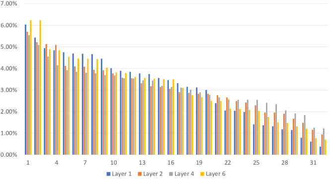
We compare the attribute distribution of tokens on different experts for different encoder layers of . The results are shown in Figure 4. The load percentages for each expert in different layers are relatively balanced.
Appendix B Computational Complexity Proof
Given a Mixture of Attention Heads with attention experts, a MoA layer has parameters. A multi-head attention layer has parameters. To compare these two complexities, we conduct the fraction of them.
We note , then we get
When , we have , and
which is a hyperbolic-like curve, with value equals to 1 when . Therefore, if , we have the proportion between the parameters of MoA and that of multi-head attention inferior to 1. Thus, the MoA layer contains fewer parameters than multi-head attention layer.
Appendix C Traning Details
| Dataset | Model | Emb Size | FFD Size | Encoder Layers | Decoder Layers |
|---|---|---|---|---|---|
| WMT14 | MoA base | 512 | 2048 | 6 | 6 |
| MoA big | 512 | 2048 | 6 | 6 | |
| Wikitext-103 | MoA | 512 | 2048 | 8 | - |
| Dataset | Model | BSZ | LR | warmup | Dropout | DropATT | DropFFD | Epochs |
|---|---|---|---|---|---|---|---|---|
| WMT14 EN-DE | MoA base | 8092 32 | 7e-4 | 4000 | 0.2 | 0.2 | 0.1 | 100 |
| MoA big | 4096 64 | 7e-4 | 4000 | 0.2 | 0.2 | 0.1 | 100 | |
| WMT14 EN-FR | MoA base | 8092 32 | 7e-4 | 8000 | 0.1 | 0 | 0.1 | 50 |
| MoA big | 4096 64 | 7e-4 | 8000 | 0.1 | 0.1 | 0.1 | 100 | |
| Wikitext-103 | MoA | 16384 32 | 6e-4 | 2000 | 0.1 | 0 | 0 | 60 |
All of our models are trained on 32 V100 GPUs. We use the Adam Optimizer (Kingma and Ba, 2015) with , and . We use a inverse square root learning rate scheduler for the translation tasks and a linear scheduler for the masked language model task. During training, we employed label smoothing (Szegedy et al., 2016) of value 0.1. More training hyperparameters can be found in Table 6.
Appendix D Utility of different auxiliary losses
We adopted two different auxiliary losses to balance the experts’ loads, one is proposed by Fedus et al. (2021), the other is proposed by Zoph et al. (2022). To validate the utility of these two auxiliary losses, we conducted several ablation tests. The results are shown in Table 7. With different combinations of auxiliary losses and different coefficients, we found that 0.01 + 0.001 achieved the best BLEU score on WMT14 EnDe test set.
| MoA | 0.01 | 0.01 | 0.001 | 0.01+0.001 | 0.01+0.01 |
|---|---|---|---|---|---|
| 28.95 | 28.73 | 28.78 | 28.94 | 28.73 | |
| 28.53 | 28.68 | 28.61 | 28.77 | 28.62 | |
| 28.45 | 28.31 | 28.38 | 28.32 | 28.4 |
Appendix E MACs calculation
ptflops launches a given model on a random tensor (with pre-defined input shapes) and estimates amount of computations (multiply-add operations) during inference. We need to define the shapes of inputs when using ptflops to calculate MACs. For translation models, we set encoder sequence length and decoder sequence length to be 10. We set the batch size to be 1. For language modeling models, we set the sequence length to be 128 and the batch size to be 1. With the pre-defined input shapes, ptflops will conduct the forward process of the given model and feed back the MACs.