The Type II-P Supernova 2019mhm and Constraints on Its Progenitor System

Abstract

We present pre- and post-explosion observations of the Type II-P supernova (SN II-P) 2019mhm located in NGC 6753. Based on optical spectroscopy and photometry, we show that SN 2019mhm exhibits broad lines of hydrogen with a velocity of $-8500\pm 200$ km s^-1 and a $111\pm 2$ day extended plateau in its luminosity, typical of the Type II-P subclass. We also fit its late-time bolometric light curve and infer that it initially produced a ⁵⁶Ni mass of $1.3\times 10^{-2}$ M${}_{\odot}\pm 5.5\times 10^{-4}$ $M_{\odot}$. Using imaging from the Wide Field Planetary Camera 2 on the Hubble Space Telescope obtained 19 years before explosion, we aligned to a post-explosion Wide Field Camera 3 image and demonstrate that there is no detected counterpart to the SN to a limit of $>$24.53 mag in F814W, corresponding to an absolute magnitude limit of $M_{\rm F814W}<-7.7$ mag. Comparing to massive-star evolutionary tracks, we determine that the progenitor star had a maximum zero-age main sequence mass $<$17.5 M_⊙, consistent with other SN II-P progenitor stars. SN 2019mhm can be added to the growing population of SNe II-P with both direct constraints on the brightness of their progenitor stars and well-observed SN properties.

1 Introduction

The core of a star of at least 8 $M_{\odot}$ will catastrophically collapse at the end of its life typically leading to a supernova (SN) (Burrows et al., 1995). Luminous supernovae (SNe) observed with hydrogen in their spectra are classified as Type II, with further sub-classifications called Type II-P, Type II-L, and Type IIb based on light curve and spectroscopic properties (Barbon et al., 1979; Filippenko, 1997; Arcavi, 2017). The most common Type II-P SNe quickly reach maximum brightness and then their luminosities tend to stay relatively constant in optical bands, resulting in a “plateau” in their light curves due to the recombination of hydrogen in their massive outer envelopes (Falk & Arnett, 1977). Nickel starts to decay into cobalt, and the SN then fades significantly to luminosities powered by radioactive ⁵⁶Co. Thus Type II-P SNe require progenitor stars with massive, extended hydrogen envelopes, which has long been taken as an indication that they arise from red supergiant (RSG) stars (Arnett, 1987; Woosley et al., 1987; Falk & Arnett, 1973).

Observations of RSG stars in the Milky Way and nearby galaxies suggest they range from ZAMS masses of 8–30 $M_{\odot}$ (Davies & Beasor, 2018; Davies et al., 2018; Davies & Beasor, 2020). Dozens of RSGs in nearby galaxies have been directly detected and confirmed as pre-explosion counterparts to Type II-P SNe (Smartt et al., 2004; Maund & Smartt, 2009; Maund, 2009; Fraser et al., 2010, 2011, 2014; Crockett et al., 2011; Elias-Rosa et al., 2011; Maund et al., 2013, 2014; Tomasella et al., 2013; Kochanek et al., 2017). All of these RSG progenitor stars have zero-age main sequence (ZAMS) masses of $<$17 M_⊙ with fewer than expected high-mass counterparts to any SN type found in pre-explosion imaging, despite expecting more massive stars given a Salpeter Initial Mass Function (the “red supergiant problem”; Smartt, 2009, 2015). Whether the SN progenitor-star mass function is actually cut off at or around 17-20 $M_{\odot}$ or there is some systematic or observational effect associated with this finding is unclear. For example, one proposed solution to the RSG problem is that some higher mass stars implode as “failed SNe,” becoming black holes producing a low-luminosity red transient with lower ejecta mass than a typical SNe (Woosley & Weaver, 1986; O’Connor & Ott, 2011; Adams et al., 2017; Piro, 2013). Other proposed solutions include the possibility that higher-mass stars shed their hydrogen envelopes and explode as other types of SNe (Smith et al., 2011; Beasor & Davies, 2016), reducing the contribution of high-mass RSGs to the SNe progenitor population.

A common assumption in addressing the red supergiant problem is that the line-of-sight extinction to the observed progenitor star is the same as the extinction inferred to the resulting SN. For example, the extinction to the progenitor star could be larger if the resulting SN destroys dust confined close to the star, or it could be smaller if the star produces dust between the time of the pre-explosion imaging and onset of the SN. Fraser et al. (2012) and Van Dyk et al. (2012) both found significant reddening for the progenitor of SN 2012aw, and concluded it was from circumstellar dust that was eventually destroyed after the explosion. However, Walmswell & Eldridge (2012) calculated additional extinction due to dust production from SN winds, but this hypothetical extinction was insufficient to explain the apparently missing high-mass stars in the red supergiant problem. It should be noted that Kochanek et al. (2012) demonstrated the physical inconsistencies when treating extinction of circumstellar material with interstellar medium material due to scattering of off-axis light in compact dust shells, potentially exaggerating the effect of extinction from this circumstellar material. Additional, well-observed examples are essential to disentangle the diversity of effects this may have on SNe and their massive progenitor stars.

There is still ambiguity on what the exact distribution of progenitors is and how high the upper mass limit can go, leaving a need for additional Type II progenitor detections and upper limits to constrain the intrinsic distribution. In this paper we present SN 2019mhm, a Type II-P SN discovered in NGC 6753 by Backyard Observatory Supernova Search (BOSS) transient survey 2019 Aug 2 13:13:21 (UT; Marples et al., 2019), located at $\alpha$ $=19^{\rm h}11^{\rm m}24^{\rm s}.06$, $\delta$ = $-57^{\circ}03^{\prime}18^{\prime\prime}.00$ (J2000), with an apparent magnitude $m_{C}=16.6$ Vega mag using a clear filter. We present optical observations of SN 2019mhm and constraints on the luminosity of its progenitor star using pre- and post-explosion Hubble Space Telescope imaging. The distance assumed for NGC 6753 is $23.4\pm 5.3$ Mpc via the fundamental plane method (Springob et al., 2014), along with an inferred distance modulus of $DM=31.85$ mag. We adopt a redshift of $z=0.01057$ (Wong et al., 2006).

2 OBSERVATIONS

2.1 Hubble Space Telescope Imaging

We obtained imaging of NGC 6753 from the Hubble Space Telescope (HST) Mikulski Archive for Space Telescopes covering the site of SN 2019mhm. The data were taken on 2000 June 22 20:26:14 using the Wide Field and Planetary Camera 2 (WFPC2) and on 2021 April 05 20:07:52 UT using the Wide Field Camera 3 (WFC3). WFPC2 observed for 320 seconds in the F814W filter and 1900 seconds in the F300W filter (Proposal ID 8645, PI Windhorst). We observed with WFC3 for 780 seconds in F814W and 710 seconds in F300X (Proposal ID 16239, PI Foley). The specific observations analyzed can be accessed via https://doi.org/10.17909/ggct-aw51 (catalog 10.17909/ggct-aw51). We then ran the files through the HST imaging and photometry pipeline hst123 (Kilpatrick et al., 2021) to align and construct drizzled frames for each unique filter and epoch. There were 148 common sources found in F814W. Using those combined images we further aligned each image using TweakReg (Avila et al., 2015), which uses a dynamic signal-to-noise threshold and a Gaussian convolution kernel with a 2.5 or 3.5 pixel full width at half maximum depending on the instrument to pick bright, isolated point sources. This resulted in a frame-to-frame alignment precision of 0.047 arcsec in right ascension and 0.036 arcsec in declination. To estimate the systematic uncertainty on our alignment procedure, we repeated the process using the same set of astrometric standards and splitting the sample randomly in half. Using half the stars to calculate a new alignment solution from WFPC2 to WFC3, we calculated the root-mean square offset in right ascension and declination between the positions of the other half of the stars in the WFC3 image and their updated positions in the aligned WFPC2 image. Repeating this process 100 times, we calculate the average root-mean square offset across each trial, which we consider to be the total systematic uncertainty in alignment. Our final alignment uncertainty is $0.36~{}({\rm stat.})+0.31~{}({\rm sys.})$ WFPC2 pixels in right ascension and $0.22~{}({\rm stat.})+0.29~{}({\rm sys.})$ WFPC2 pixels in declination. We obtained photometry of all sources near the site of SN 2019mhm using dolphot (Dolphin, 2016). The pre- and post-explosion F814W images centered on the site of SN 2019mhm are shown in Figure 1.

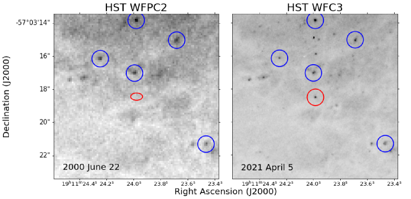
Figure 1: WFPC2 and WFC3 imaging of a 10.0${}^{\prime\prime}\times$ 10.0^′′ region centered around where we would expect to see the pre-explosion counterpart to SN 2019mhm, taken 2000 June 22 (pre-explosion,left) and WFC3 imaging of a region around SN 2019mhm taken 2021 April 05 (post-explosion, right). Both images are using the HST F814W filter. The location of SN 2019mhm is outlined by a red ellipse at $20\sigma$ in the left panel, and circled in red in the right panel. 5 additional point sources are circled in blue.

2.2 Imaging of SN 2019mhm

We observed SN 2019mhm in $uBV\!gri$ bands with the Swope 1-m optical telescope at Las Campanas Observatory, Chile from 2 August 2019 to 14 March 2020. All data were calibrated using bias and flat-field frames observed in the same instrumental configuration as described in Kilpatrick et al. (2018) and using the photpipe imaging and photometry package (Rest et al., 2005). We used photpipe to perform amplifier crosstalk corrections, masking, astrometric calibration, photometry using a custom version of DoPhot (Schechter et al., 1993), and photometric calibration using SkyMapper photometric standards (Onken et al., 2020) observed in the same field as SN 2019mhm. Finally, using deep template imaging obtained on 9–10 October 2021, we performed image subtraction using hotpants (Becker, 2015) and forced photometry on the position of SN 2019mhm using a custom version of DoPhot.

SN 2019mhm was also observed in $BVg^{\prime}r^{\prime}i^{\prime}$ bands by the Sinistro imagers on the Las Cumbres Observatory (LCO) 1-m telescope network from 2019 August 2 to 2020 March 2. Starting from the pixel-level calibrated imaging provided by the LCO BANZAI pipeline (McCully et al., 2018), we performed all masking, astrometric, and photometric calibration following identical methods to those described above for the Swope imaging. We then used the final epoch of $BVg^{\prime}r^{\prime}i^{\prime}$ LCO imaging obtained on 2020 June 18 as templates to perform image subtraction with hotpants and obtained forced photometry with DoPhot. The final forced-photometry of SN 2019mhm from our Swope and LCO difference images is shown in Table 1 and Figure 2.

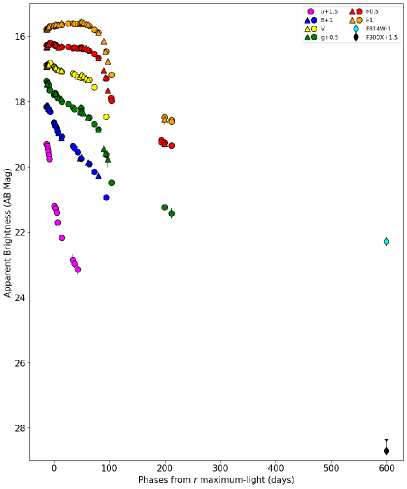
Figure 2: Light curves of SN 2019mhm from HST (diamonds), LCO (triangles), and Swope (circles) photometry of SN 2019mhm covering $uBVgri$, F814W, and F300X. Dates are reported with respect to maximum-light in the $r$ band.

2.3 Spectroscopy of SN 2019mhm

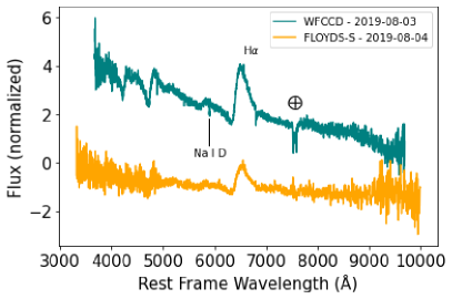
Figure 4: Spectra of SN 2019mhm in WFCCD and FLOYDS-S. The H-$\alpha$ line, Na I D line, and Telluric feature are highlighted.

We obtained the classification spectrum of SN 2019mhm for our spectral analysis (as described in Chen et al., 2019). These data were obtained at Las Campanas Observatory with the du Pont 2.5m telescope and Wide field reimaging CCD (WFCCD) on 3 August 2019. All data were processed following standard procedures in IRAF, including flattening, aperture extraction, wavelength calibration, and flux calibration. In addition, we analyzed spectroscopy of SN 2019mhm obtained through the Las Cumbres Observatory (LCO) network at Siding Spring Observatory, Australia on the Faulkes 2m telescope and FLOYDS spectrograph from 4 August 2019. We reduced these data with the LCO FLOYDS pipeline (Valenti et al., 2013) using arc and flat-field frames obtained on the same night and in the same instrumental configuration. The final spectra are shown in Figure 4.

3 Methods and Results

3.1 Spectroscopic and Extinction Properties of SN 2019mhm

The spectra of SN 2019mhm exhibit broad lines of H$\alpha$ and H$\beta$, which combined with its peak magnitude and light-curve evolution highlight its nature as a Type II-P SN. For the Milky Way, we use the reddening value of $E(B-V)=0.06$ mag from Schlafly & Finkbeiner (2011). Below we assume that the total-to-selective extinction in NGC 6753 is $R_{V}=A_{V}/E(B-V)=3.1$ (Cardelli89), similar to the Milky Way.

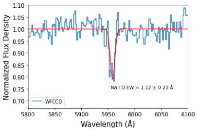
Figure 5: Na I D doublet in WFCCD spectrum of 2019mhm. The equivalent width of the doublet is $1.12\pm 0.20$ Å.

It is possible to determine the internal extinction from the EW of the Na ID absorption line at the host galaxy redshift. To infer the Na i D equivalent width, we first removed the recessional velocity of NGC 6753 and normalized the continuum emission in the WFCCD spectrum. We masked the wavelength range around the Na i D doublet centroid (near $\lambda\lambda$5889.95, 5895.92). We then masked the continuum around the centroid, and we fit a Gaussian profile to the Na i D absorption profile. The resulting equivalent width was $1.12\pm 0.20$ Å, as shown in Figure 5. To convert this quantity to a reddening value, we used the relation between Na i D column density and extinction presented in Phillips et al. (2013). We adopt a host-galaxy reddening value to be $E(B-V)=0.180\begin{subarray}{c}+0.036\\ -0.029\end{subarray}$ mag assuming $R_{V}=3.1$ for the following analyses.

We performed a similar analysis to calculate the velocity of the much broader H$\alpha$ line. Here we masked the wavelength range around $\lambda$ = 6563 Å. We calculate the velocity to be $-8500\pm 200$ km s^-1 at the absorption minimum. This velocity is consistent with those measured from other Type II SNe around or slightly before maximum light, for example well-observed events such as SNe 1986L, 1999em ($9820$ km s^-1), and 2012aw ($12800$ km s^-1; Bose et al., 2013) used to infer distances via the expanding photosphere method (Schmidt et al., 1994; Leonard et al., 2002; Bose & Kumar, 2014).

3.2 The Bolometric Light Curve of SN 2019mhm

Our multi-band light curves of SN 2019mhm are shown in Figure 2, which track the evolution of this event from 12 hours to 612 days from discovery. We ran all light curves through superbol (Nicholl et al., 2016) to integrate the time-varying spectral energy distribution (SED) of SN 2019mhm and obtain a bolometric light curve by integrating the black body fits of the SEDs over all wavelengths. We determined a bolometric luminosity at each $i$-band epoch, and performed a linear interpolation on the other light curves to that epoch to construct the full SED. We used a distance modulus value of $31.85$ mag and a reddening value of $E(B-V)=0.24$ mag as mentioned above when running the photometry through superbol, and we did not impose any UV suppression as our observations do not extend blueward of $u$-band.

The final epoch for SN 2019mhm was 612.845 days, corresponding to a rest-frame epoch of 606 days. We searched the Weizmann Interactive Supernova Data Repository (WISseREP; Yaron & Gal-Yam, 2012) for spectra of other SNe IIP with rest-frame epochs between 525 and 675 days, and found a single spectrum for the Type II-P SN 2004dj at 665 rest-frame days from explosion. From this spectrum, we used pysynphot (STScI Development Team, 2013) to calculate a pseudo-bolometric magnitude and in-band magnitude for F814W and thus a pseudo-bolometric correction for that band, which we estimate to be $BC_{{\rm F814W}}=0.35$ mag. This value is in agreement within the errors of our superbol analysis assuming no color evolution from the previous epoch, which results in $BC_{{\rm F814W}}=-0.2\pm 0.8$ mag. We adopt $BC_{{\rm F814W}}=0.35$ mag for the analysis below.

We then plotted the bolometric light curve with respect to time from explosion for SN 2019mhm using the assuming the time of explosion was the discovery date in MJD, plotted in Figure 6. We used the emcee package (Foreman-Mackey et al., 2013) to infer the plateau duration using equation 1 from Valenti et al. (2016).The decline rate of SN 2019mhm closely tracks expectations for a ⁵⁶Co-powered light curve (with a $\approx 0.012$ mag day^-1 decline as in Valenti et al., 2016). This is at both $200$ days from explosion when deep ground-based observations were still possible and out to 610 days from explosion as observed by HST. We can therefore scale the bolometric light curve of SN 2019mhm to other well-observed SNe such as SN 1987A (e.g., Spiro et al., 2014) to infer the total ⁵⁶Ni mass produced in the event. Using equation 3 of Spiro et al. (2014) and interpolating the bolometric luminosities of SN 2019mhm and SN 1987A at 200 days from explosion, we derive a ⁵⁶Ni mass of $1.3\times 10^{-2}$ $M_{\odot}\pm 5.5\times 10^{-4}$ $M_{\odot}$.

We compare SN 2019mhm’s bolometric light curve to those of other Type II SNe in Figure 6, including SN 2017gmr (Andrews et al., 2019), SN 1987A (Terreran et al., 2017; Suntzeff90; Hamuy90), SN 2013ej (Yuan et al., 2016), and SN 2012aw (Dall’Ora et al., 2014). SN  2019mhm is still brighter and with a higher ⁵⁶ Ni mass than the objects belonging to the family of ’faint’ or ’low-luminosity’ Type II-P SNe (Spiro et al., 2014).

3.3 Constraints on a pre-explosion counterpart to SN 2019mhm

We identified SN 2019mhm in a single post-explosion WFC3 F814W image, and consider a counterpart to be a source within a 3$\sigma$ radius of SN 2019mhm’s location. We did not find any counterpart within 3$\sigma$ alignment precision of that location in pre-explosion WFPC2 F814W imaging (Figure 1). There are seven point-like sources within a 5″ radius of the explosion site of WFPC2 imaging, the closest of which is approximately 1.1″ (41$\sigma$ astrometric uncertainty) away and detected at $m_{\rm F814W}=22.6$ mag. We therefore consider there to be no pre-explosion counterpart to SN 2019mhm in the WFPC2 imaging, and below we infer the upper limit on the flux to any counterpart in the pre-explosion data.

Using the deeper WFC3 F814W frame as a reference image for all sources detected in both the WFC3 and WFPC2 data, we obtained photometry of point sources in the individual flattened frames (flc/c0m) using dolphot (Dolphin, 2016). We derived the upper limit on the presence of a point-like source in pre-explosion WFPC2 frames by injecting various sources with magnitudes from 19 to 26 mag into the individual flat frames at the location of SN  2019mhm. Based on the non-detection of a source in the WFPC2 frames, we derived an upper limit on the presence of a counterpart by analyzing sources detected at $\geq$3$\sigma$ significance within 20^′′ of the location of SN 2019mhm. This estimate implies that in the pre-explosion image, any counterpart to SN 2019mhm must have had $m_{\rm F814W}>24.53$ mag (AB). We show the evolutionary tracks of stars with various masses in Figure 3. In the post-explosion image (roughly 1.6 yr after discovery), we derive $m_{\rm F814W}=23.28\pm 0.04$ mag (AB) for SN 2019mhm itself (Table 1 and Figure 2).

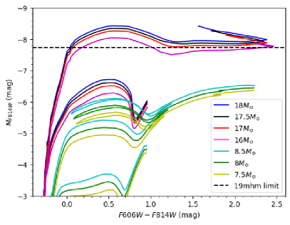
Figure 3: Evolutionary tracks of various stellar masses. The absolute limit of SN  2019mhm is noted in blue.

Using the limits on progenitor flux along with the distance modulus, Milky Way extinction and extinction in the host galaxy, we considered giant star tracks and the in-band luminosities of these stars right before explosion. We compared our limits to the MESA Isochrones and Stellar Tracks (MIST) models (Choi et al., 2017), and we found that our F814W explosion limit rules out all terminal RSGs with ZAMS masses $>$17.5 $M_{\odot}$.

The limit we derived is comparable to the upper limits for RSG progenitors presented in Smartt (2009, 2015), but more recent analyses suggest that the mass limit is actually higher than 18 $M_{\odot}$. Davies & Beasor (2018) argue that systematic error leads to a significant underestimation of progenitor star masses, and present a cutoff at 25 $M_{\odot}$, with an upper limit of $<33~{}M_{\odot}$ at 2$\sigma$ confidence. Davies & Beasor (2020) suggest that the lower mass limit is 6-8 $M_{\odot}$, and the upper mass limit between 18-20 $M_{\odot}$. It should be noted that as a whole, the sample size for detected progenitor stars is rather small, making the analysis of SNe like SN 2019mhm important to help build up statistics. We present the masses of RSG stars in the literature in Figure 7.

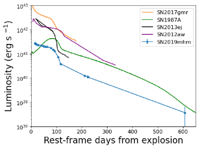
Figure 6: Bolometric light curves of Type II-P SNe.

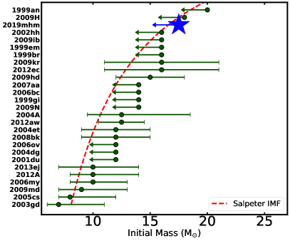
Figure 7: Masses of RSG progenitor stars in the literature, with a Salpeter IMF truncated at 8 and 24 $M_{\odot}$.

4 Discussion & Conclusions

SN 2019mhm can be added to the current sample of direct detections and upper limits used to analyze the Type II SN progenitor mass function, currently at 26 SNe (Smartt, 2015). Based on the methods described above, we derived a ZAMS mass limit of 17.5 $M_{\odot}$. This further constrains the mass threshold at which Type II-P SNe can explode from RSGs as likely being below 18 $M_{\odot}$ assuming a Salpeter IMF. Indeed, Davies & Beasor (2018) argue that the “upper mass” threshold for the RSG counterparts to SNe II may not be statistically significant with an upper mass limit that is consistent with the maximum mass RSG at the 3$\sigma$ level (i.e., at the Humphreys-Davidson limit of $\approx$30 $M_{\odot}$; Humphreys & Davidson, 1979).

Following methods in Davies & Beasor (2020), we analyzed the Type II progenitor star photometry presented in that paper to evaluate the effect of adding SN 2019mhm on that analysis. In summary, this analysis takes the progenitor star photometry, extinction, distance, and bolometric correction for each detected source and upper limit (24 total in Davies & Beasor, 2020) and estimates the most likely observed progenitor star luminosity distribution by varying each of these quantities within their reported uncertainties. It then compares this distribution to an empirical luminosity power-law distribution with a power-law index ($\Gamma$), lower luminosity cutoff ($L_{\rm low}$) and upper luminosity cutoff ($L_{\rm high}$). This analysis removes systematic biases in translating from RSG luminosity to initial mass and can be compared directly to the observed luminosities of RSGs in the Milky Way and other galaxies.

Following this analysis, we derive a lower and upper luminosity cutoffs of $\log(L_{\rm low}/L_{\odot})=4.43\begin{subarray}{c}+0.09\\ -0.10\end{subarray}$ and $\log(L_{\rm high}/L_{\odot})=5.23\begin{subarray}{c}+0.14\\ -0.10\end{subarray}$, with nominally smaller uncertainties than in Davies & Beasor (2020) but consistent with their analysis. When we added our limits on SN 2019mhm and re-ran this analysis, we found these values changed to $\log(L_{\rm low}/L_{\odot})=4.43\begin{subarray}{c}+0.07\\ -0.10\end{subarray}$ and $\log(L_{\rm high}/L_{\odot})=5.21\begin{subarray}{c}+0.12\\ -0.10\end{subarray}$, in agreement with the previous analysis although with a moderately lower $L_{\rm high}$ value and smaller uncertainties.

Analyzing every nearby SN with pre-explosion imaging is essential to building a large, unbiased population of progenitor systems and understand the causes of the RSG problem (Smartt, 2015). Another possible solution to the RSG problem is that dust shells surrounding these stars obscure them, and as a result their luminosities and masses are severely underestimated. However, it was shown that the luminosities of these progenitors in the X-ray luminosities were not high enough to prove this was the case (Dwarkadas, 2014). The conclusion that dust obscuration significantly lowers the inferred luminosities of these red supergiants assumes that the circumstellar material is extended around the progenitor star, whereas some Type II progenitors are known to have compact circumstellar shells (Kilpatrick & Foley, 2018).

5 Acknowledgements

We thank Ben Davies for providing progenitor luminosity code and helpful comments on our analysis. We also thank Jorge Anais Vilchez, Abdo Campillay, Yilin Kong-Riveros, Nahir Muñoz-Elgueta and Natalie Ulloa for observations on the Swope Telescope at Las Campanas Observatory, Chile. We thank Tom Holoien and Subo Dong for providing raw duPont data. This material is based upon work supported by the National Science Foundation under grant No.1757792,a Research Experiences for Undergraduates (REU) grant awarded to CIERA at Northwestern University. Any opinions, findings, and conclusions or recommendations expressed in this material are those of the author(s) and do not necessarily reflect the views of the National Science Foundation.

Table 1: Photometry of SN 2019mhm

MJD	Filter	$m$	$\sigma_{m}$	Source
		(mag)	(mag)
58698.0523	$B$	$>$17.151	–	Swope
58699.1103	$B$	17.195	0.015	Swope
58700.1585	$B$	17.203	0.014	Swope
58701.0631	$B$	17.248	0.017	Swope
58702.0586	$B$	17.244	0.019	Swope
58703.0934	$B$	17.296	0.027	Swope
58704.1889	$B$	17.317	0.021	Swope
58711.0576	$B$	17.647	0.044	Swope
58712.0317	$B$	17.686	0.029	Swope
58713.0139	$B$	17.742	0.020	Swope
58714.0861	$B$	17.757	0.028	Swope
58716.0392	$B$	17.820	0.017	Swope
58718.0530	$B$	17.920	0.017	Swope
58725.0228	$B$	18.070	0.017	Swope
58745.0505	$B$	18.356	0.026	Swope
58748.0183	$B$	18.424	0.019	Swope
58753.9984	$B$	18.546	0.021	Swope
58760.0564	$B$	18.753	0.104	Swope
58775.0350	$B$	18.918	0.031	Swope
58784.0457	$B$	19.157	0.027	Swope
58805.0251	$B$	19.936	0.059	Swope
58698.0512	$V$	16.881	0.017	Swope
58699.1082	$V$	16.866	0.018	Swope
58699.1092	$V$	16.874	0.017	Swope
58700.1573	$V$	16.899	0.016	Swope
58701.0620	$V$	16.896	0.018	Swope
58702.0575	$V$	16.845	0.023	Swope
58703.0924	$V$	16.846	0.025	Swope
58704.1877	$V$	16.832	0.020	Swope
58711.0564	$V$	16.925	0.037	Swope
58712.0302	$V$	16.939	0.023	Swope
58713.0127	$V$	16.981	0.019	Swope
58714.0848	$V$	16.989	0.030	Swope
58716.0361	$V$	17.024	0.015	Swope
58718.0519	$V$	17.029	0.017	Swope
58725.0214	$V$	17.087	0.015	Swope
58745.0480	$V$	17.148	0.019	Swope
58748.0158	$V$	17.169	0.016	Swope
58753.9963	$V$	17.249	0.016	Swope
58760.0537	$V$	17.269	0.088	Swope
58775.0328	$V$	17.335	0.024	Swope
58784.0435	$V$	17.558	0.019	Swope
58805.0224	$V$	18.472	0.032	Swope
58698.0449	$g$	16.869	0.018	Swope
58699.1019	$g$	16.932	0.016	Swope
58700.1502	$g$	16.933	0.014	Swope
58701.0563	$g$	16.954	0.016	Swope
58702.0518	$g$	17.024	0.021	Swope
58703.0864	$g$	17.159	0.051	Swope
58704.1860	$g$	17.165	0.022	Swope
58711.0547	$g$	17.292	0.052	Swope
58712.0233	$g$	17.243	0.025	Swope
58713.0111	$g$	17.234	0.018	Swope
58714.0780	$g$	17.280	0.025	Swope
58716.0275	$g$	17.334	0.014	Swope
58718.0453	$g$	17.378	0.016	Swope
58725.0128	$g$	17.495	0.015	Swope
58737.2121	$g$	17.575	0.020	Swope
58745.0377	$g$	17.677	0.021	Swope
58748.0039	$g$	17.745	0.015	Swope
58760.0507	$g$	17.707	0.137	Swope
58761.0173	$g$	17.787	0.024	Swope
58775.0306	$g$	17.993	0.027	Swope
58784.0408	$g$	18.191	0.019	Swope
58791.0157	$g$	18.355	0.042	Swope
58805.0197	$g$	19.122	0.039	Swope
58815.0265	$g$	19.982	0.049	Swope
58910.3514	$g$	20.738	0.090	Swope
58923.4080	$g$	20.927	0.165	Swope
58698.0439	$i$	16.783	0.018	Swope
58699.1003	$i$	16.779	0.017	Swope
58700.1489	$i$	16.782	0.016	Swope
58701.0553	$i$	16.739	0.017	Swope
58702.0508	$i$	16.729	0.020	Swope
58703.0854	$i$	16.708	0.035	Swope
58704.1850	$i$	16.686	0.019	Swope
58711.0535	$i$	16.676	0.034	Swope
58712.0211	$i$	16.687	0.022	Swope
58713.0098	$i$	16.665	0.018	Swope
58714.0769	$i$	16.670	0.018	Swope
58716.0257	$i$	16.681	0.015	Swope
58718.0442	$i$	16.654	0.015	Swope
58725.0115	$i$	16.644	0.015	Swope
58737.2043	$i$	16.603	0.014	Swope
58745.0352	$i$	16.611	0.016	Swope
58748.0013	$i$	16.616	0.014	Swope
58753.9862	$i$	16.617	0.017	Swope
58760.0493	$i$	16.616	0.109	Swope
58775.0284	$i$	16.678	0.017	Swope
58784.0385	$i$	16.789	0.017	Swope
58791.0141	$i$	16.883	0.028	Swope
58805.0178	$i$	17.464	0.024	Swope
58815.0216	$i$	18.184	0.027	Swope
58910.3439	$i$	19.481	0.051	Swope
58923.3903	$i$	19.567	0.111	Swope
58923.4006	$i$	19.618	0.050	Swope
58698.0429	$r$	16.769	0.016	Swope
58699.0991	$r$	16.788	0.017	Swope
58700.1475	$r$	16.765	0.014	Swope
58701.0543	$r$	16.752	0.016	Swope
58702.0498	$r$	16.760	0.020	Swope
58703.0844	$r$	16.726	0.023	Swope
58704.1840	$r$	16.693	0.018	Swope
58711.0525	$r$	16.736	0.030	Swope
58712.0199	$r$	16.759	0.018	Swope
58713.0086	$r$	16.781	0.018	Swope
58714.0747	$r$	16.755	0.018	Swope
58716.0237	$r$	16.800	0.014	Swope
58718.0432	$r$	16.805	0.014	Swope
58725.0093	$r$	16.821	0.014	Swope
58737.1967	$r$	16.822	0.014	Swope
58745.0327	$r$	16.857	0.016	Swope
58747.9988	$r$	16.845	0.013	Swope
58753.9848	$r$	16.876	0.015	Swope
58760.0480	$r$	16.830	0.048	Swope
58761.0138	$r$	16.831	0.055	Swope
58775.0263	$r$	16.946	0.017	Swope
58784.0355	$r$	17.043	0.015	Swope
58791.0124	$r$	17.162	0.023	Swope
58805.0157	$r$	17.791	0.021	Swope
58814.0250	$r$	18.388	0.023	Swope
58815.0165	$r$	18.472	0.028	Swope
58904.3849	$r$	19.675	0.073	Swope
58904.3857	$r$	19.748	0.029	Swope
58910.3363	$r$	19.759	0.033	Swope
58923.3827	$r$	19.845	0.044	Swope
58923.3931	$r$	19.853	0.039	Swope
58698.0459	$u$	17.799	0.018	Swope
58699.1031	$u$	17.865	0.017	Swope
58700.1515	$u$	17.948	0.016	Swope
58701.0574	$u$	18.025	0.019	Swope
58702.0528	$u$	18.135	0.025	Swope
58703.0875	$u$	18.266	0.037	Swope
58712.0248	$u$	19.705	0.108	Swope
58714.0795	$u$	19.774	0.085	Swope
58716.0295	$u$	19.905	0.042	Swope
58718.0468	$u$	20.204	0.052	Swope
58725.0141	$u$	20.666	0.071	Swope
58745.0402	$u$	21.357	0.181	Swope
58748.0069	$u$	21.463	0.138	Swope
58753.9889	$u$	21.638	0.181	Swope
58697.8094	$B$	17.114	0.028	LCO
58698.6828	$B$	17.115	0.026	LCO
58698.6845	$B$	17.138	0.027	LCO
58699.7424	$B$	17.111	0.027	LCO
58701.2949	$B$	17.207	0.032	LCO
58713.8128	$B$	17.709	0.030	LCO
58719.1947	$B$	17.956	0.031	LCO
58724.1995	$B$	18.105	0.031	LCO
58757.8405	$B$	18.743	0.047	LCO
58760.7363	$B$	18.704	0.046	LCO
58772.7468	$B$	18.867	0.050	LCO
58791.0465	$B$	19.269	0.100	LCO
58697.8117	$V$	16.929	0.025	LCO
58698.6864	$V$	16.896	0.026	LCO
58698.6877	$V$	16.910	0.026	LCO
58699.7448	$V$	16.889	0.025	LCO
58701.2972	$V$	16.873	0.024	LCO
58713.8147	$V$	16.967	0.025	LCO
58719.1966	$V$	17.032	0.024	LCO
58724.2014	$V$	17.038	0.020	LCO
58757.8436	$V$	17.226	0.023	LCO
58760.7394	$V$	17.170	0.023	LCO
58764.7429	$V$	17.220	0.023	LCO
58768.7399	$V$	17.276	0.027	LCO
58772.7499	$V$	17.327	0.026	LCO
58698.6893	$g$	16.967	0.022	LCO
58698.6910	$g$	16.952	0.021	LCO
58713.8161	$g$	17.243	0.025	LCO
58719.1980	$g$	17.391	0.025	LCO
58724.2028	$g$	17.417	0.024	LCO
58757.8453	$g$	17.808	0.027	LCO
58760.7410	$g$	17.826	0.026	LCO
58764.7446	$g$	17.850	0.028	LCO
58772.7515	$g$	17.983	0.028	LCO
58791.0491	$g$	18.357	0.043	LCO
58801.0107	$g$	18.950	0.115	LCO
58803.7668	$g$	19.094	0.126	LCO
58808.0161	$g$	19.263	0.272	LCO
58697.8082	$i$	16.782	0.037	LCO
58698.6957	$i$	16.778	0.046	LCO
58698.6971	$i$	16.770	0.043	LCO
58699.7413	$i$	16.718	0.030	LCO
58701.2937	$i$	16.708	0.031	LCO
58709.9815	$i$	16.673	0.032	LCO
58713.8189	$i$	16.625	0.030	LCO
58719.2008	$i$	16.643	0.025	LCO
58724.2056	$i$	16.596	0.024	LCO
58757.8487	$i$	16.573	0.027	LCO
58760.7445	$i$	16.539	0.025	LCO
58764.7480	$i$	16.577	0.025	LCO
58768.7450	$i$	16.614	0.027	LCO
58772.7550	$i$	16.625	0.031	LCO
58791.0523	$i$	16.888	0.030	LCO
58801.0130	$i$	17.142	0.039	LCO
58803.7691	$i$	17.459	0.086	LCO
58808.0189	$i$	17.761	0.049	LCO
58910.3803	$i$	19.541	0.173	LCO
58697.8105	$r$	16.841	0.023	LCO
58698.6928	$r$	16.830	0.023	LCO
58698.6942	$r$	16.811	0.022	LCO
58699.7436	$r$	16.755	0.023	LCO
58701.2960	$r$	16.733	0.021	LCO
58713.8176	$r$	16.759	0.021	LCO
58719.1995	$r$	16.835	0.021	LCO
58724.2043	$r$	16.803	0.018	LCO
58757.8473	$r$	16.849	0.022	LCO
58760.7430	$r$	16.830	0.019	LCO
58764.7466	$r$	16.880	0.021	LCO
58768.7436	$r$	16.866	0.022	LCO
58772.7535	$r$	16.901	0.021	LCO
58791.0508	$r$	17.165	0.025	LCO
58801.0119	$r$	17.536	0.035	LCO
58803.7680	$r$	17.760	0.048	LCO
58808.0176	$r$	18.157	0.042	LCO
58910.3762	$r$	19.797	0.087	LCO
59309.8452	F814W	23.282	0.039	HST
59309.8515	F300X	27.202	0.368	HST

Note. — Photometry of SN 2019mhm from HST, the Swope 1m telescope, and Las Cumbres Observatory (LCO) 1m telescopes. All photometry is on the AB mag system.

References

- Adams et al. (2017) Adams, S. M., Kochanek, C. S., Gerke, J. R., Stanek, K. Z., & Dai, X. 2017, MNRAS, 468, 4968
- Andrews et al. (2019) Andrews, J. E., Sand, D. J., Valenti, S., et al. 2019, ApJ, 885, 43
- Arcavi (2017) Arcavi, I. 2017, Hydrogen-Rich Core-Collapse Supernovae, ed. A. W. Alsabti & P. Murdin, 239
- Arnett (1987) Arnett, W. D. 1987, ApJ, 319, 136
- Avila et al. (2015) Avila, R. J., Hack, W., Cara, M., et al. 2015, in Astronomical Society of the Pacific Conference Series, Vol. 495, Astronomical Data Analysis Software an Systems XXIV (ADASS XXIV), ed. A. R. Taylor & E. Rosolowsky, 281
- Barbon et al. (1979) Barbon, R., Ciatti, F., & Rosino, L. 1979, A&A, 72, 287
- Beasor & Davies (2016) Beasor, E. R., & Davies, B. 2016, Monthly Notices of the Royal Astronomical Society, 463, 1269. https://doi.org/10.1093/mnras/stw2054
- Becker (2015) Becker, A. 2015, HOTPANTS: High Order Transform of PSF ANd Template Subtraction, , , ascl:1504.004
- Bose & Kumar (2014) Bose, S., & Kumar, B. 2014, ApJ, 782, 98
- Bose et al. (2013) Bose, S., Kumar, B., Sutaria, F., et al. 2013, MNRAS, 433, 1871
- Burrows et al. (1995) Burrows, A., Hayes, J., & Fryxell, B. A. 1995, ApJ, 450, 830
- Chen et al. (2019) Chen, P., Holoien, T. W. S., & Dong, S. 2019, Transient Name Server Classification Report, 2019-1444, 1
- Choi et al. (2017) Choi, J., Conroy, C., & Byler, N. 2017, ApJ, 838, 159
- Crockett et al. (2011) Crockett, R. M., Smartt, S. J., Pastorello, A., et al. 2011, MNRAS, 410, 2767
- Dall’Ora et al. (2014) Dall’Ora, M., Botticella, M. T., Pumo, M. L., et al. 2014, ApJ, 787, 139
- Davies & Beasor (2018) Davies, B., & Beasor, E. R. 2018, MNRAS, 474, 2116
- Davies & Beasor (2020) —. 2020, MNRAS, 493, 468
- Davies et al. (2018) Davies, B., Crowther, P. A., & Beasor, E. R. 2018, MNRAS, 478, 3138
- Dolphin (2016) Dolphin, A. 2016, DOLPHOT: Stellar photometry, , , ascl:1608.013
- Dwarkadas (2014) Dwarkadas, V. V. 2014, Monthly Notices of the Royal Astronomical Society, 440, 1917. https://doi.org/10.1093/mnras/stu347
- Elias-Rosa et al. (2011) Elias-Rosa, N., Van Dyk, S. D., Li, W., et al. 2011, ApJ, 742, 6
- Falk & Arnett (1973) Falk, S. W., & Arnett, W. D. 1973, ApJ, 180, L65
- Falk & Arnett (1977) —. 1977, ApJS, 33, 515
- Filippenko (1997) Filippenko, A. V. 1997, ARA&A, 35, 309
- Foreman-Mackey et al. (2013) Foreman-Mackey, D., Hogg, D. W., Lang, D., & Goodman, J. 2013, PASP, 125, 306
- Fraser et al. (2010) Fraser, M., Takáts, K., Pastorello, A., et al. 2010, ApJ, 714, L280
- Fraser et al. (2011) Fraser, M., Ergon, M., Eldridge, J. J., et al. 2011, MNRAS, 417, 1417
- Fraser et al. (2012) Fraser, M., Maund, J. R., Smartt, S. J., et al. 2012, ApJ, 759, L13
- Fraser et al. (2014) —. 2014, MNRAS, 439, L56
- Humphreys & Davidson (1979) Humphreys, R. M., & Davidson, K. 1979, ApJ, 232, 409
- Kilpatrick & Foley (2018) Kilpatrick, C. D., & Foley, R. J. 2018, MNRAS, 481, 2536
- Kilpatrick et al. (2018) Kilpatrick, C. D., Foley, R. J., Drout, M. R., et al. 2018, MNRAS, 473, 4805
- Kilpatrick et al. (2021) Kilpatrick, C. D., Drout, M. R., Auchettl, K., et al. 2021, MNRAS, 504, 2073
- Kochanek et al. (2012) Kochanek, C. S., Khan, R., & Dai, X. 2012, ApJ, 759, 20
- Kochanek et al. (2017) Kochanek, C. S., Fraser, M., Adams, S. M., et al. 2017, MNRAS, 467, 3347
- Leonard et al. (2002) Leonard, D. C., Filippenko, A. V., Gates, E. L., et al. 2002, PASP, 114, 35
- Marples et al. (2019) Marples, P., Bock, G., & Pearl, P. 2019, Transient Name Server Discovery Report, 2019-1393, 1
- Maund (2009) Maund, J. R. 2009, in American Institute of Physics Conference Series, Vol. 1111, Probing Stellar Populations Out to the Distant Universe: Cefalu 2008, Proceedings of the International Conference, ed. G. Giobbi, A. Tornambe, G. Raimondo, M. Limongi, L. A. Antonelli, N. Menci, & E. Brocato, 291–298
- Maund et al. (2014) Maund, J. R., Reilly, E., & Mattila, S. 2014, MNRAS, 438, 938
- Maund & Smartt (2009) Maund, J. R., & Smartt, S. J. 2009, Science, 324, 486
- Maund et al. (2013) Maund, J. R., Fraser, M., Smartt, S. J., et al. 2013, MNRAS, 431, L102
- McCully et al. (2018) McCully, C., Volgenau, N. H., Harbeck, D.-R., et al. 2018, in Society of Photo-Optical Instrumentation Engineers (SPIE) Conference Series, Vol. 10707, Software and Cyberinfrastructure for Astronomy V, ed. J. C. Guzman & J. Ibsen, 107070K
- Nicholl et al. (2016) Nicholl, M., Berger, E., Margutti, R., et al. 2016, ApJ, 828, L18
- O’Connor & Ott (2011) O’Connor, E., & Ott, C. D. 2011, ApJ, 730, 70
- Onken et al. (2020) Onken, C. A., Wolf, C., Bessell, M. S., et al. 2020, arXiv e-prints, arXiv:2008.10359
- Phillips et al. (2013) Phillips, M. M., Simon, J. D., Morrell, N., et al. 2013, ApJ, 779, 38
- Piro (2013) Piro, A. L. 2013, ApJ, 768, L14
- Rest et al. (2005) Rest, A., Stubbs, C., Becker, A. C., et al. 2005, ApJ, 634, 1103
- Schechter et al. (1993) Schechter, P. L., Mateo, M., & Saha, A. 1993, PASP, 105, 1342
- Schlafly & Finkbeiner (2011) Schlafly, E. F., & Finkbeiner, D. P. 2011, ApJ, 737, 103
- Schmidt et al. (1994) Schmidt, B. P., Kirshner, R. P., Eastman, R. G., et al. 1994, ApJ, 432, 42
- Smartt (2009) Smartt, S. J. 2009, ARA&A, 47, 63
- Smartt (2015) —. 2015, PASA, 32, e016
- Smartt et al. (2004) Smartt, S. J., Maund, J. R., Hendry, M. A., et al. 2004, Science, 303, 499
- Smith et al. (2011) Smith, N., Li, W., Filippenko, A. V., & Chornock, R. 2011, Monthly Notices of the Royal Astronomical Society, 412, 1522. https://doi.org/10.1111/j.1365-2966.2011.17229.x
- Spiro et al. (2014) Spiro, S., Pastorello, A., Pumo, M. L., et al. 2014, MNRAS, 439, 2873
- Springob et al. (2014) Springob, C. M., Magoulas, C., Colless, M., et al. 2014, MNRAS, 445, 2677
- STScI Development Team (2013) STScI Development Team. 2013, pysynphot: Synthetic photometry software package, Astrophysics Source Code Library, record ascl:1303.023, , , ascl:1303.023
- Terreran et al. (2017) Terreran, G., Pumo, M. L., Chen, T. W., et al. 2017, Nature Astronomy, 1, 713
- Tomasella et al. (2013) Tomasella, L., Cappellaro, E., Fraser, M., et al. 2013, MNRAS, 434, 1636
- Valenti et al. (2013) Valenti, S., Sand, D., & Howell, D. A. 2013
- Valenti et al. (2016) Valenti, S., Howell, D. A., Stritzinger, M. D., et al. 2016, MNRAS, 459, 3939
- Van Dyk et al. (2012) Van Dyk, S. D., Cenko, S. B., Poznanski, D., et al. 2012, ApJ, 756, 131
- Walmswell & Eldridge (2012) Walmswell, J. J., & Eldridge, J. J. 2012, MNRAS, 419, 2054
- Wong et al. (2006) Wong, O. I., Ryan-Weber, E. V., Garcia-Appadoo, D. A., et al. 2006, MNRAS, 371, 1855
- Woosley et al. (1987) Woosley, S. E., Pinto, P. A., Martin, P. G., & Weaver, T. A. 1987, ApJ, 318, 664
- Woosley & Weaver (1986) Woosley, S. E., & Weaver, T. A. 1986, ARA&A, 24, 205
- Yaron & Gal-Yam (2012) Yaron, O., & Gal-Yam, A. 2012, PASP, 124, 668
- Yuan et al. (2016) Yuan, F., Jerkstrand, A., Valenti, S., et al. 2016, MNRAS, 461, 2003