Tackling Instance-Dependent Label Noise with Dynamic Distribution Calibration

Abstract.

Instance-dependent label noise is realistic but rather challenging, where the label-corruption process depends on instances directly. It causes a severe distribution shift between the distributions of training and test data, which impairs the generalization of trained models. Prior works put great effort into tackling the issue. Unfortunately, these works always highly rely on strong assumptions or remain heuristic without theoretical guarantees. In this paper, to address the distribution shift in learning with instance-dependent label noise, a dynamic distribution-calibration strategy is adopted. Specifically, we hypothesize that, before training data are corrupted by label noise, each class conforms to a multivariate Gaussian distribution at the feature level. Label noise produces outliers to shift the Gaussian distribution. During training, to calibrate the shifted distribution, we propose two methods based on the mean and covariance of multivariate Gaussian distribution respectively. The mean-based method works in a recursive dimension-reduction manner for robust mean estimation, which is theoretically guaranteed to train a high-quality model against label noise. The covariance-based method works in a distribution disturbance manner, which is experimentally verified to improve the model robustness. We demonstrate the utility and effectiveness of our methods on datasets with synthetic label noise and real-world unknown noise.

1. Introduction

Learning with label noise is one of the hottest topics in weakly-supervised learning (Han et al., 2020; Lukasik et al., 2020; Collier et al., 2021). In real life, large-scale datasets are likely to contain label noise. The main reason is that manual high-quality labeling is expensive (Northcutt et al., 2021; Ortego et al., 2021; Wu et al., 2021a). Large-scale datasets are always collected from crowdsourcing platforms (Li et al., 2017) or crawled from the internet (Yao et al., 2020), which inevitably introduces label noise.

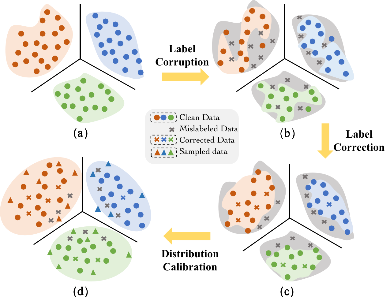
Figure 1. The illustrations of the distribution-shift problem and our solution. The background color areas represent the data distributions of different classes. (a) This represents clean data and ground-truth data distributions. (b) Due to label corruption, partial data are mislabeled, resulting in noisy labels. The distributions trained on data with noisy labels mismatch to ground-truth distributions. (c) Label correction mainly corrects data far from decision boundaries. However, the mislabeled data near decision boundaries are still not corrected, making learned distributions biased. (d) By using our distribution calibration, the learned distributions are closer to ground-truth distributions, naturally following better generalization abilities.

Instance-dependent label noise (Cheng et al., 2020a; Xia et al., 2020; Cheng et al., 2020b) is more realistic and applicable than instance-independent label noise, where the label-flipping process depends on instances/features directly. It is because, in real-world scenes, an instance whose features contain less discriminative information or are of poorer quality may be more likely to be mislabeled. Instance-dependent label noise is more challenging owing to its inherent complexity (Zhu et al., 2021). Compared with instance-independent label noise, it leads to a more severe distribution shift problem for trained models (Berthon et al., 2021). That is to say, this kind of noise makes the distributions of training and test data significantly different. If the models are trained with instance-dependent label noise, it is pessimistic that they would generalize poorly on test data (Xia et al., 2022b).

The recent methods on handling instance-dependent label noise are generally divided into two main categories. The first one is to estimate the instance-dependent transition matrix (Xia et al., 2020; Jiang et al., 2022; Xia et al., 2022a), which tends to characterize the behaviors of clean labels flipping into noisy labels. However, these methods are limited to the case with a small number of classes (Zhu et al., 2021; Xia et al., 2019). Besides, they highly rely on strong assumptions to achieve an accurate estimation, e.g., the assumptions on anchor points, bounded noise rates, and extra trusted data. It is hard or even infeasible to check these assumptions, which hinders the validity of these methods (Jiang et al., 2022). The second one tends to heuristically identify clean data based on the memorization effect of deep models (Arpit et al., 2017) for subsequent operations, e.g., label correction (Tanaka et al., 2018; Zheng et al., 2020; Tanaka et al., 2018). Unfortunately, due to the complexity of instance-dependent label noise, label correction will be much weaker in the noisy region near the decision boundary. Therefore, the labels corrected by the current predictions would likely be erroneous (Berthon et al., 2021). In addition, the training data in identified clean regions in this way is relatively monotonous (Xia et al., 2022b; Pleiss et al., 2020). The corresponding distribution will be restricted to a small region of the global distribution, which introduces covariate shift (Sugiyama and Kawanabe, 2012). We detail the above issues in Figure 1. Therefore, the methods belonging to both two categories cannot well handle the distribution shift brought by instance-dependent label noise.

In this paper, to address the above issues, we propose a dynamic distribution-calibration strategy. We first assume that, before training data are corrupted by label noise, each class conforms to a multivariate Gaussian distribution at the feature level. Such an assumption is more reasonable and has been verified in lots of works, such as (Hernández-Lobato et al., 2014; Kendall and Gal, 2017). Then, two methods based on the mean and covariance of multivariate Gaussian distributions are proposed. Specifically, the mean-based method works in a recursive dimension-reduction manner, which is theoretically guaranteed to train a high-quality model against instance-dependent label noise. It first assigns smaller weights to outliers and then divides the whole feature space into clean space and corrupted space where the contamination has larger effects on corrupted space. We recurse the computation on corrupted space for robust mean estimation. The covariance-based method works in a distribution disturbance manner, which is experimentally verified. It introduces an interference in the empirical covariance of given data. In this way, we can increase the diversity of training data to mitigate the distribution shift and improve generalization. After achieving multivariate Gaussian distributions for all classes, we sample examples from them for training, which calibrates the shifted distributions.

We conduct extensive experiments across various settings on CIFAR-10, CIFAR-100, WebVision, and Clothing1M. The results consistently exhibit substantial performance improvements compared to state-of-the-art methods, which support our claims well.

Organization. The rest of this paper is organized as follows. In Section 2, we introduce some background knowledge. In Section 3, we present our methods step by step, with theoretical justifications. In Section 4, empirical evaluations are provided. In Section 5, we summarize this paper.

Figure 2. The noise level curve of PMD noise. The red curve represents the upper bound. The noise level is bounded by $\rho$ in the restricted region while unbounded in the unrestricted region. The blue curve shows the actual noise level.

2. Preliminaries

Notations. Let $\mathbbm{I}[\mathcal{A}]$ be the indicator of the event $\mathcal{A}$. Let $[z]=\{0,\ldots,z-1\}$. Besides, $|\mathcal{B}|$ denotes the total number of elements in the set $\mathcal{B}$.

Problem setup. We consider a $k$-classification problem ($k\geq 2$). Let $\mathcal{X}$ and $\mathcal{Y}=[k]$ be the instance and class label spaces respectively. We assume the dataset $\{(\bm{x}_{i},y_{i})\}_{i=1}^{n}$ is sampled from the underlying joint distribution $\mathcal{D}$ over $\mathcal{X}\times\mathcal{Y}$, where $n$ is the sample size. Before observation, partial clean labels are flipped due to instance-dependent label noise. As a result, we are provided with a noisy training dataset $\{(\bm{x}_{i},\tilde{y}_{i})\}_{i=1}^{n}$ obtained from a noisy joint distribution $\tilde{\mathcal{D}}$ over $\mathcal{X}\times\mathcal{Y}$. For each instance $\bm{x}_{i}$, its label $\tilde{y}_{i}$ may be incorrect. Our goal is to learn a robust classifier by only exploiting the noisy dataset, which can assign clean labels to test data precisely.

Label noise model. In this paper, we consider polynomial-margin diminishing noise (PMD noise) (Zhang et al., 2021b). The PMD noise is one of the instance-dependent label noise, which is realistic but rather challenging. Although the noise setting and analyses naturally generalize to the multi-class case ($k>2$), for simplicity, we first focus on the binary case ($k=2$) to improve legibility. Specifically, let $\eta(\bm{x})=\mathbbm{P}(y=1|\bm{x})$ be the clean class posterior. Let $\rho_{0,1}(\bm{x})=\mathbbm{P}[\tilde{y}=1|y=0,\bm{x}]$ and $\rho_{1,0}(\bm{x})=\mathbbm{P}[\tilde{y}=0|y=1,\bm{x}]$ be the noise functions where $\tilde{y}$ denotes the noisy label. For example, an instance $\bm{x}$ has the true label $y=0$, the noisy label is flipped to $1$ with the probability of $\rho_{0,1}(\bm{x})$. We give the formal definition of PMD noise as follows.

Definition 0 (PMD noise).

The noise functions $\rho_{0,1}(\bm{x})$ and $\rho_{1,0}(\bm{x})$ are PMD, if there are constants $0<t_{0}<\frac{1}{2}$ and $c_{1},c_{2}>0$ such as

(1) $$\rho_{0,1}(\bm{x})\leq c_{1}\eta(\bm{x})^{1+c_{2}};\forall\eta(\bm{x})\leq\frac{1}{2}-t_{0};$$

(2) $$\rho_{1,0}(\bm{x})\leq c_{1}[1-\eta(\bm{x})]^{1+c_{2}};\forall\eta(\bm{x})\geq\frac{1}{2}+t_{0}.$$

We denote $t_{0}$ as the margin of $\rho$. In the restricted region $\{\bm{x}:|\eta(\bm{x})-\frac{1}{2}|>t_{0}\}$, the PMD noise requires the upper bound on $\rho$ to be polynomial and monotonically decreasing (Zhang et al., 2021b). Meanwhile, in the unrestricted region $\{\bm{x}:|\eta(\bm{x})-\frac{1}{2}|<t_{0}\}$, both $\rho_{0,1}$ and $\rho_{1,0}$ can be arbitrary. For a clearer understanding, Figure 2 provides the noise level curve of the PMD noise. The PMD noise is consistent with real-world noisy scenarios: data near the decision boundary is hard to distinguish and likely to be mislabeled so the noise level can be arbitrary. Meanwhile, data far away from the decision boundary owns typical features of its class so the noise level should be bounded.

3. Methodology

In this section, we present our methods step by step. We first show how to extract the deep features of instances based on label correction and how to model deep features (Section 3.1). Then, we detail the mean-based method (Section 3.2) and covariance-based method (Section 3.3). Lastly, the theoretical analysis is provided to justify our claims (Section 3.4).

3.1. Feature Extraction and Label Correction

Given a training example $(\bm{x},\tilde{y})$, we employ a deep network to finish the encoding and classification for it. In more detail, first, the instance $\bm{x}$ is fed into the deep network to obtain its deep features, which are denoted by $h(\bm{x})\in\mathbbm{R}^{d}$. Then, we map the deep features to the class label space with the classifier $f(h(\bm{x}))$. For simplicity, we use $f(\bm{x})$ to substitute $f(h(\bm{x}))$. In binary classification, $f(x):\mathcal{X}\rightarrow[0,1]$. Let $y_{f(\bm{x})}:=\mathbbm{I}(f(\bm{x})\geq\frac{1}{2})$ be the label predicted by $f$.

In this paper, we build our methods based on label correction (Zhang et al., 2021b), mainly considering its sample-efficiency (Tanaka et al., 2018). Specifically, we first warm up the deep network within a few epochs. The warm-up phase is used to initialize the model for the following operations. Then, we correct the label, where $f$ has high confidence in it. With a threshold $\tau$, if $|f(\bm{x})-\frac{1}{2}|>\tau$, we flip $\tilde{y}$ to the prediction $y_{f(\bm{x})}$ of $f$. We repeatedly correct labels and improve the network within the epoch, until no label can be corrected. In the next epoch, we sightly relax the threshold $\tau$ for label correction. The above procedure can be easily extended to the multi-class scenario (see Appendix B for more details).

Recall that we assume that before training data are corrupted by label noise, the features of each class conform to a multivariate Gaussian distribution. That is, for $k$ classes, we define $k$ multivariate Gaussian distributions in total. The distribution for the $c$-th class is denoted by $\mathcal{N}_{c}(h(\bm{x})|\bm{\mu}^{c},\bm{\Sigma}^{c})$, where $\bm{\mu}^{c}\in\mathbbm{R}^{d}$ and $\bm{\Sigma}^{c}\in\mathbbm{R}^{d\times d}$.

Note that when all deep feature distributions are ideal, i.e., they are not corrupted by label noise, the empirical mean $\bar{\bm{\mu}}^{c}$ is well-known to be an optimal estimator of the true mean $\bm{\mu}^{c}$ at most $\mathcal{O}(\sqrt{d/n_{c})}$, where $n_{c}$ is the number of examples belonging to the $c$-th class. The existence of label noise makes the empirical mean fail: even a single corrupted data can arbitrarily mislead the mean estimation. However, as discussed, the label correction approach cannot handle distribution shift caused by instance-dependent label noise in two aspects: (1) The labels corrected by the current predictions would likely be erroneous; (2) The training data in identified clean regions in this way is relatively monotonous, leading to covariate shift. The two issues motivate us to explore more robust solutions.

3.2. Mean-Based Method

Based on the Huber’s contamination model (Huber, 1992) and our assumption, we introduce the algorithm AgnosticMean (Lai et al., 2016). In summary, the algorithm consists of two steps: (1) the outlier damping step; (2) the projection step. In the outlier damping step, we assign different weights to each data point where outliers will get smaller weights. In the projection step, we project data points onto the span (denoted as $\mathcal{V}$) of the top $\frac{d}{2}$ principal components. Two steps are alternately implemented to achieve robust mean estimation, which mitigates the side effect of instance-dependent label noise. In the following, we give mathematical descriptions of our mean-based method.

Given the noisy dataset $\{(\bm{x}_{i},\tilde{y}_{i})\}_{i=1}^{n}$, after label correction at the $t$-th epoch, we obtain the dataset $\{(\bm{x}_{i},\tilde{y}_{i}^{t})\}_{i=1}^{n}$. For building the multivariate Gaussian distribution on deep features $h(\bm{x})$, we take instances whose labels are $c$ as examples, the rest classes are the same procedure. We group these instances into a set $\mathcal{S}$. Due to the corruption caused by label noise, we have $\mathcal{S}=\mathcal{S}_{\mathcal{N}}\cup\mathcal{S}_{\mathcal{Q}}$, where $\mathcal{S}_{\mathcal{N}}$ and $\mathcal{S}_{\mathcal{Q}}$ include the instances sampled from the underlying multivariate Gaussian distribution and arbitrary noise distribution respectively. If the noise rate is $\epsilon$, we have $|\mathcal{S}_{\mathcal{Q}}|=\epsilon|\mathcal{S}|$. We assume that the underlying distribution is $\mathcal{N}(h(\bm{x})|\bm{\mu},\sigma^{2}\bm{I})$. Note that the assumption on the covariance is practical in statistical/machine learning and related tasks (c.f.  (Kingma and Welling, 2013; Kingma et al., 2016; Diakonikolas and Kane, 2019)). The notations $\bm{\mu}_{\mathcal{S}}$ (resp. $\bm{\mu}_{\mathcal{Q}}$) and $\bm{\Sigma}_{\mathcal{S}}$ (resp. $\bm{\Sigma}_{\mathcal{Q}}$) denote the mean and covariance of the set $\mathcal{S}$ (resp. $\mathcal{S}_{\mathcal{Q}}$). We then have

(3) $$\bm{\Sigma}_{\mathcal{S}}=(1-\epsilon)\sigma^{2}\bm{I}+\epsilon\bm{\Sigma}_{\mathcal{Q}}+\epsilon(1-\epsilon)(\bm{\mu}_{\mathcal{\mathcal{S}}}-\bm{\mu}_{\mathcal{Q}})(\bm{\mu}_{\mathcal{S}}-\bm{\mu}_{\mathcal{Q}})^{\top}.$$

Our main goal is to find the mean shift, i.e., $\bm{\mu}_{\mathcal{S}}-\bm{\mu}$. The rationality behind this is that if outliers substantially move $\bm{\mu}_{\mathcal{S}}$ far away from $\bm{\mu}$, it must move $\bm{\mu}_{\mathcal{S}}$ in the direction of $\bm{\mu}_{\mathcal{S}}-\bm{\mu}$. The outlier damping step can effectively limit the effect of outliers. The projection step contributes to find the direction of the mean shift.

Outlier damping step. In this step, we impose different weights on different instances. Specifically, the instances that are far away from the coordinate-wise median are endowed with smaller weights. Here, the coordinate-wise median simply takes the median in each dimension. Subsequently, we use $\bm{m}$ to denote the coordinate-wise median of $\mathcal{S}$. Let $s^{2}=C\textsf{Tr}(\bm{\Sigma}_{\mathcal{S}})$, where $C$ is a constant, $\textsf{Tr}(\bm{\Sigma}_{\mathcal{S}})$ is the trace of $\bm{\Sigma}_{\mathcal{S}}$. The weight of each instance can be obtained by the following equation:

(4) $$\omega_{i}=\exp(-\frac{||h(\bm{x}_{i})-\bm{m}||_{2}^{2}}{s^{2}}),\bm{x}_{i}\in\mathcal{S}.$$

After obtaining different weights of all instances, we reset the covariance of the set $\mathcal{S}$ with the weights. That is,

(5) $$\bm{\Sigma}_{\mathcal{S},\bm{\omega}}=\sum\omega_{i}\frac{(h(\bm{x}_{i})-\bm{\mu}_{\mathcal{S},\bm{\omega}})(h(\bm{x}_{i})-\bm{\mu}_{\mathcal{S},\bm{\omega}})^{\top}}{n_{c}},$$

where $\bm{\mu}_{\mathcal{S},\bm{\omega}}=\sum\omega_{i}\frac{h(\bm{x}_{i})}{n_{c}}$ and $n_{c}$ denotes the number of examples belonging to the $c$-th class.

Projection step. With the aim of containing a large projection of $\bm{\mu}_{\mathcal{S}}-\bm{\mu}$, we project $\mathcal{S}$ onto the span $\mathcal{V}$ of the top $\frac{d}{2}$ principal components of $\bm{\Sigma}_{\mathcal{S,\bm{\omega}}}$. For the span of the bottom $\frac{d}{2}$ principal components (denoted as $\mathcal{W}$). $\mathcal{P}_{\mathcal{W}}\bm{\mu}$ is just approximated by $\mathcal{P}_{\mathcal{W}}\bm{\mu}_{\mathcal{S}}$, where $\mathcal{P}_{\mathcal{W}}$ represents the operation projecting to the space $\mathcal{W}$. After determining the projection of $\bm{\mu}$ in space $\mathcal{W}$, we still need to ensure the mean in space $\mathcal{V}$. We recursively perform the outlier damping step and projection step in $\mathcal{V}$. To the end, there will be only a one-dimensional space which is treated as the direction of $\bm{\mu}_{\mathcal{S}}-\bm{\mu}$. Note that when the dimension of deep features is 1, the median of $\mathcal{S}$ is known to be a robust estimator of the mean with the error of $\mathcal{O}(\epsilon\sigma)$ (Huber, 2004; Hampel et al., 2011). So we just compute the median as the robust mean estimator.

Figure 3 illutrates the effectiveness of the mean-based method. After the outlier damping step, outliers are assigned with smaller weights. The mean shift $\bm{\mu}_{\mathcal{S}}-\bm{\mu}$ onto the space $\mathcal{W}$ has very small projection, which implies that the contribution of outliers in space $\mathcal{W}$ on average cancels out and the sample mean leads to a small error. Therefore, we just need to perform the outlier damping step and projection step in space $\mathcal{V}$ at the next procedure until there is only one dimension. The procedure of the algorithm AgnosticMean is presented in Algorithm 1. Emphatically, Steps 4-6 belong to outlier damping. Step 7 belongs to projection. In Step 8, the outlier damping and projection steps are performed recursively, until there will be only a one-dimensional space. The procedure of AgnosticMean is executed for any $c-$th class to obtain its robust mean $\hat{\bm{\mu}}^{c}$. We will provide theoretical insights for the mean-based method in Section 3.4.

Algorithm 1 AgnosticMean

0:  The set $\mathcal{S}=\{h(\bm{x}_{1}),\ldots,h(\bm{x}_{n_{c}})\}$ with $h(\bm{x}_{i})\in\mathbbm{R}^{d}$.

1:  if $d=1$  then

2:     return  median($\mathcal{S}$).

3:  end if

4:  Let $s^{2}=C\textsf{Tr}(\bm{\Sigma}_{\mathcal{S}})$;

5:  Compute the weight $\omega_{i}$ for every $h(\bm{x_{i}})\in\mathcal{S}$ with Eq. (4), $\bm{\omega}=(\omega_{1},...,\omega_{n_{c}})$;

6:  Reset the covariance of the set $\mathcal{S}$ as $\bm{\Sigma}_{\mathcal{S},\bm{\omega}}$ with Eq. (5);

7:  Project $\mathcal{S}$ onto the span $\mathcal{V}$ and $\mathcal{W}$ to obtain $\mathcal{P}_{\mathcal{V}}\mathcal{S}$ and $\mathcal{P}_{\mathcal{W}}\mathcal{S}$, $\mathcal{P}_{\mathcal{V}}\mathcal{S}\in\mathbbm{R}^{\frac{d}{2}}$, $\mathcal{P}_{\mathcal{W}}\mathcal{S}\in\mathbbm{R}^{\frac{d}{2}}$;

8:  Set $\bm{\hat{\mu}}_{\mathcal{V}}$ = AgnosticMean($\mathcal{P}_{\mathcal{V}}\mathcal{S}$) recursively and $\bm{\hat{\mu}}_{\mathcal{W}}$ = mean($\mathcal{P}_{\mathcal{W}}\mathcal{S}$);

9:  Obtain $\bm{\hat{\mu}}\in\mathbbm{R}^{d}$, where $\mathcal{P}_{\mathcal{V}}\bm{\hat{\mu}}=\bm{\hat{\mu}}_{\mathcal{V}}$ and $\mathcal{P}_{\mathcal{W}}\bm{\hat{\mu}}=\bm{\hat{\mu}}_{\mathcal{W}}$.

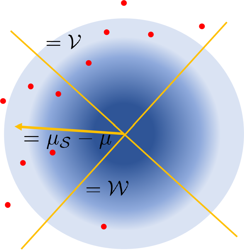
Figure 3. The illustration of the mean-based method. The circular area is the data space where the color depth degree indicates the weights of data. The points in the darker region will be assigned larger weights. The red points are outliers and the orange arrow represents the direction of the mean shift.

3.3. Covariance-Based Method

As discussed, if we exploit the memorization effect of deep networks (Arpit et al., 2017), the training data in identified clean regions in this way is relatively monotonous, leading to covariate shift. In other words, the training data in identified clean regions are sampled from a biased distribution and cannot cover the underlying distribution well (Wang et al., 2019b; Li et al., 2022; Yang et al., 2021).

To relieve the above issue, we add some disturbance to the empirical covariance of the biased distribution. Intuitively, in this way, we can increase the diversity of training data to mitigate the overfitting to the biased distribution. Specifically, for any $c$-th class, we first compute the mean and covariance of the corresponding distribution of the $c$-th class, i.e.,

$$\hat{\bm{\mu}}=\sum\frac{h(\bm{x}_{i})}{n_{c}},$$

(6) $$\hat{\bm{\Sigma}}=\sum\frac{\left(h(\bm{x}_{i})-\hat{\bm{\mu}}\right)\left(h(\bm{x}_{i})-\hat{\bm{\mu}}\right)^{\top}}{n_{c}}.$$

Then, we add the disturbance to the covariance $\hat{\bm{\Sigma}}$, which can expand the features’ regions, rendering the model gains robustness against covariate shift. That is,

(7) $$\hat{\bm{\Sigma}}^{*}=\sum\frac{\left(h(\bm{x}_{i})-\hat{\bm{\mu}}\right)\left(h(\bm{x}_{i})-\hat{\bm{\mu}}\right)^{\top}}{n_{c}}+\alpha\mathbf{1},$$

where $\alpha\in\mathbbm{R}^{+}$ is a hyperparameter that controls the degree of the disturbance, and $\mathbf{1}\in\mathbbm{R}^{d\times d}$ is a matrix of ones. Note that it is rather hard to set an optimal $\alpha$ from a theoretical view. It is because, without strong assumptions, the determination of the optimal covariance is an open problem in robust statistics. Therefore, in this paper, we determine the value of $\alpha$ by simply employing a (noisy) validation set. Experimental results prove the feasibility of this way.

Algorithm flow. We present the overall paradigm of our methods in Algorithm 2. For the setting of $\tau(t)$, we follow the setting in (Zhang et al., 2021b). In summary, we first use warm-up training to make the model predictions more reliable (Step 1). Then, in each epoch, we exploit label correction to obtain a corrected dataset (Steps 3-7) for the following extraction of deep features (Step 8). Next, we perform the proposed two methods (described in Section 3.2 and 3.3) to build multivariate Gaussian distributions for all classes (Steps 9-11). At last, extra data points are sampled from the built multivariate Gaussian distributions for training, which finishes the distribution calibration to improve generalization (Steps 12-15). In this work, we name our methods with label correction as mean-based dynamic distribution calibration (MDDC) and covariance-based dynamic distribution calibration (CDDC) respectively.

Algorithm 2 The algorithm flow of our methods

0:  The noisy dataset $\{(\bm{x}_{i},\tilde{y}_{i})\}_{i=1}^{n}$, the maximum of the training epoch $t_{\max}$, the number of warm up $t_{w}$, the threshold $\tau(t)$, the initial classifier $f$, and the sampled fraction $\lambda$.

1:  Warm up the classifier $f$ on $\{(\bm{x}_{i},\tilde{y}_{i})\}_{i=1}^{n}$ within $t_{w}$ epochs;

2:  for  $t=t_{w}+1,...,t_{max}$ do

3:     for all $(\bm{x}_{i},\tilde{y}_{i}^{t-1})\in\{(\bm{x}_{i},\tilde{y}_{i}^{t-1})\}_{i=1}^{n}$ and $|f(\bm{x}_{i})-\frac{1}{2}|\geq\tau(t)$ do

4:        $\tilde{y}_{i}^{t}\leftarrow\mathbbm{1}_{\{f(\bm{x}_{i})\geq\frac{1}{2}\}}$//label correction;

5:     end for

6:     Obtain the corrected dataset $\{(\bm{x}_{i},\tilde{y}_{i}^{t})\}_{i=1}^{n}$;

7:     Train $f$ on the corrected dataset;

8:     Extract the deep features of all instances, i.e., $h(\bm{x}_{i})$;

9:     for $c$ = 1, …, $k$ do

10:        Build multivariate Gaussian distributions for the $c$-th class using the mean-based or covariance-based method;

11:     end for

12:     Sample extra examples from all $k$ multivariate Gaussian distributions with the number of $\lambda n$//data sampling;

13:     Train $f$ on the sampled examples;

14:  end for

15:  return  Trained classifier $f$.

3.4. Theoretical Analysis

We provide theoretical analyses of MDDC based on PLC (Zhang et al., 2021b), which shows that a classifier trained with our strategy converges to be consistent with the Bayes optimal classifier with high probability. In this work, we focus on the asymptotic case (Mohri et al., 2018).

Pre-knowledge. For completeness, we first reproduce the relevant background knowledge.

Definition 0 ($(\beta,v)$-consistency (Zhang et al., 2021b)).

Suppose that a set of data $(\bm{x},\tilde{y})$ are sampled from $\tilde{\mathcal{D}}(\bm{x},\tilde{\eta}(\bm{x}))$, where $\tilde{\eta}(\bm{x})$ outputs the noisy posterior probability for $\bm{x}$. Given a hypothesis class $\mathcal{M}$ with sufficient examples, and $f(\bm{x})=\mathop{\arg\min}\limits_{m\in\mathcal{M}}\mathbb{E}_{(\bm{x},\tilde{y})\sim\tilde{\mathcal{D}}(\bm{x},\tilde{\eta}(\bm{x}))}Loss(m(x),\tilde{y})$, we define $\mathcal{M}$ is $(\beta,v)$-consistency if

(8) $$|f(\bm{x})-\eta(\bm{x})|\leq$$

$$\beta\mathbbm{E}_{(\bm{z},\tilde{y})\sim\tilde{\mathcal{D}}(\bm{z},\tilde{\eta}(\bm{z}))}\big{[}\mathbbm{1}_{\{\tilde{y}_{\bm{z}}\neq\eta^{*}(\bm{z})\}}(\bm{z})\big{|}|\eta(\bm{z})-\frac{1}{2}|\geq|\eta(\bm{x})-\frac{1}{2}|\big{]}+v,$$

where $\eta(\bm{z})$ outputs the clean posterior probability for $\bm{z}$ and $\eta^{*}(\bm{z})$ is the Bayes optimal classifier for $\bm{z}$.

Definition 1 measures the inconsistency between $f(\cdot)$ and $\eta(\cdot)$. We can approximate the error of the classifier $f$ at $\bm{x}$ by computing the risk of $\eta^{*}(\cdot)$ at $\bm{z}$ where $\eta^{*}(\bm{z})$ are more confident than $\eta^{*}(\bm{x})$.

Definition 0 ($c_{*},c^{*})$-bounded distribution (Zhang et al., 2021b)).

Denote the cumulative distribution function of $|\eta(\bm{x})-\frac{1}{2}|$ as $R(\cdot)$. For a random variable $o$, $R(o)=\mathbbm{P}(|\eta(\bm{x})-\frac{1}{2}|\leq o)$ and the corresponding probability density function is $r(o)$. We define the distribution $\mathcal{D}$ is ($c_{*},c^{*})$-bounded if $0<c_{*}\leq r(o)\leq c^{*}$ for all $0\leq o\leq\frac{1}{2}$. The worst-case density-imbalance ratio of $\mathcal{D}$ is denoted by $\ell:=\frac{c^{*}}{c_{*}}$.

The bounded condition enforces the continuity of the density function. The continuity allows one example to borrow useful information from its (clean) neighborhood region, which can help handle mislabeled data.

Definition 0 (Pure ($\tau,f,\eta$)-level set).

We say a set $S(\tau,\eta):=\big{\{}\bm{x}\big{|}|\eta(\bm{x})-\frac{1}{2}|\geq\tau\big{\}}$ is pure for the classifier $f$, if $y_{f(\bm{x})}=\eta^{*}(\bm{x})$ for all $\bm{x}\in S(\tau,\eta)$, where $y_{f(\bm{x})}$ denotes the label predicted by $f$, i.e., $y_{f(\bm{x})}=\mathbbm{1}_{\{f(\bm{x})\geq\frac{1}{2}\}}$.

The above definition indicates that the classifier $f$ has sufficient discriminating ability in a specific region.

Assumption. We present the following assumption for theoretical results.

Assumption 1.

We assume that the given hypothesis class $\mathcal{M}$ is $(\beta,v)$-consistency, and the underlying distribution $\mathcal{D}$ satisfied the $(c^{*},c_{*})$-bounded condition.

Theoretical results. Based on the above pre-knowledge and assumption, we formally present our theoretical results.

Lemma 0 (One round purity improvement).

Suppose that the classifier $f$ owns a pure ($\tau,f,\eta$)-level set where $3\xi v\leq\tau<\frac{1}{2}$, where $\xi<1$ is a constant that depends on the PMD noise. After one round label correction (described in Section 3.1) and one round sampling from estimated Gaussian distributions (described in Sections 3.2 and 3.3), the training set consists of two parts: the corrected set ($\bm{x}$, $\tilde{y}_{new})$ and the sampling set ($\bm{x}$, $\tilde{y}_{\mathcal{G}}$). Training on these data, $f$ owns a improved pure ($\tau_{new},f,\eta$)-level set where $\frac{1}{2}-\tau_{new}\geq(1+\frac{\xi v}{\beta\ell})(\frac{1}{2}-\tau)$.

Theorem 5.

After training on the noisy dataset, the proposed method will return the trained classifier $f$ such that

(9) $$\mathbb{P}_{\bm{x}\sim\tilde{\mathcal{D}}}[y_{f(\bm{x})}=\eta^{*}(\bm{x})]\geq 1-3\xi c^{*}v.$$

The proofs are provided in Appendix A. Lemma 4 tells us that the cleansed region will be enlarged by at least a constant factor after one training round. Theorem 5 states that the classifier trained with our method converges to be consistent with the Bayes optimal classifier with high probability. Note that since $\xi<1$, $1-3\xi c^{*}v>1-3c^{*}v$ holds, which indicates our method can help the classifier converge to be consistent with the Bayes optimal classifier with a higher probability than PLC (Zhang et al., 2021b). The theoretical results verify the effectiveness of our method well. In the next section, we use comprehensive experiments to support our claims.

4. Experiments

In this section, we first introduce the used baselines in this paper (Section 4.1). The evaluations on synthetic and real-world label-noise datasets are then provided (Section 4.2 and 4.3). Finally, a comprehensive ablation study is provided (Section 4.4).

4.1. Baselines

In this paper, we compare our methods with five representative baselines and implement all methods with default parameters by PyTorch. The baselines include: (i). Standard; (ii). Co-teaching+ (Yu et al., 2019); (iii). GCE (Zhang and Sabuncu, 2018); (iv). SL (Wang et al., 2019a); (v). LRT (Zheng et al., 2020). The details of the above baselines are provided in Appendix C.

As our methods finish distribution calibration after label correction using PLC (Zhang et al., 2021b), we compare our methods with PLC later (Section 4.3 and Section 4.4). In this way, we can demonstrate the improvement brought by our methods more systematically and clearly. Note that we do not directly compare the proposed methods with some state-of-the-art methods, e.g., DivideMix (Li et al., 2020). It is because, DivideMix is an aggregation of multiple advanced techniques, e.g., Mixup, soft labels, and semi-supervised learning. Therefore, the comparison is not fair. In this paper, to make a fair comparison, as did in (Xia et al., 2022b), we will boost DivideMix with our methods. More details will be provided shortly.

Table 1. Mean and standard deviations of test accuracy (%) on two synthetic noisy datasets. The best two mean results are in bold.

Dataset	Noise	Standard	Co-teaching+	GCE	SL	LRT	MDDC	CDDC
CIFAR-10	Type-I (35%)	78.11$\pm$0.74	79.97$\pm$0.15	80.65$\pm$0.39	79.76$\pm$0.72	80.98$\pm$0.80	83.12$\pm$0.44	83.17$\pm$0.43
	Type-I (70%)	41.98$\pm$1.96	40.69$\pm$1.99	36.52$\pm$1.62	36.29$\pm$0.66	41.52$\pm$4.53	43.70$\pm$0.91	45.14$\pm$1.11
	Type-II (35%)	76.65$\pm$0.57	77.35$\pm$0.44	77.60$\pm$0.88	77.92$\pm$0.89	80.74$\pm$0.25	80.59$\pm$0.19	80.76$\pm$0.25
	Type-II (70%)	45.57$\pm$1.12	45.44$\pm$0.64	40.30$\pm$1.46	41.11$\pm$1.92	44.67$\pm$3.89	47.06$\pm$0.41	48.10$\pm$1.74
	Type-III (35%)	76.89$\pm$0.79	78.38$\pm$0.67	79.18$\pm$0.61	78.81$\pm$0.29	81.08$\pm$0.35	82.02$\pm$0.23	81.58$\pm$0.07
	Type-III (70%)	43.32$\pm$1.00	41.90$\pm$0.86	37.10$\pm$0.59	38.49$\pm$1.46	44.47$\pm$1.23	46.31$\pm$0.92	47.92$\pm$1.28
CIFAR-100	Type-I (35%)	57.68$\pm$0.29	56.70$\pm$0.71	58.37$\pm$0.18	55.20$\pm$0.33	56.74$\pm$0.34	63.12$\pm$0.40	62.89$\pm$0.20
	Type-I (70%)	39.32$\pm$0.43	39.53$\pm$0.28	40.01$\pm$0.71	40.02$\pm$0.85	45.29$\pm$0.43	48.32$\pm$0.85	47.78$\pm$0.53
	Type-II (35%)	57.83$\pm$0.25	56.57$\pm$0.52	58.11$\pm$1.05	56.10$\pm$0.73	57.25$\pm$0.68	63.84$\pm$0.23	64.57$\pm$0.41
	Type-II (70%)	39.30$\pm$0.32	36.84$\pm$0.39	37.75$\pm$0.46	38.45$\pm$0.45	43.71$\pm$0.51	48.41$\pm$0.96	47.74$\pm$0.62
	Type-III (35%)	56.07$\pm$0.79	55.77$\pm$0.98	57.51$\pm$1.16	56.04$\pm$0.74	56.57$\pm$0.30	63.60$\pm$0.33	63.46$\pm$0.23
	Type-III (70%)	40.01$\pm$0.38	35.37$\pm$2.65	40.53$\pm$0.60	39.94$\pm$0.84	44.41$\pm$0.19	47.42$\pm$0.17	47.04$\pm$0.34

Table 2. Mean and standard deviations of test accuracy (%) on two balanced noisy datasets. Here, the label noise is mixed by instance-dependent and class-dependent noise. The noise levels of three kinds of instance-dependent label noise are 35%. The real noise levels range from 50% to 70% lastly, since class-dependent noise is overlayed on the instance-dependent one. The best two mean results are in bold.

Dataset	Noise	Standard	Co-teaching+	GCE	SL	LRT	MDDC	CDDC
CIFAR-10	Type-I + 30% Sym.	75.26$\pm$0.32	78.72$\pm$0.53	78.08$\pm$0.66	77.79$\pm$0.46	75.97$\pm$0.27	81.35$\pm$0.13	80.66$\pm$0.09
	Type-I + 60% Sym.	64.25$\pm$0.78	55.49$\pm$2.11	67.43$\pm$1.43	67.63$\pm$1.36	59.22$\pm$0.74	74.13$\pm$0.26	74.26$\pm$0.58
	Type-I + 30% Asym.	75.21$\pm$0.64	75.43$\pm$2.96	76.91$\pm$0.56	77.14$\pm$0.70	76.96$\pm$0.45	78.85$\pm$0.35	79.12$\pm$0.21
	Type-II + 30% Sym.	74.92$\pm$0.63	75.19$\pm$0.54	75.69$\pm$0.21	75.08$\pm$0.47	75.94$\pm$0.58	79.01$\pm$0.32	79.31$\pm$0.57
	Type-II + 60% Sym.	64.02$\pm$0.66	59.89$\pm$0.63	66.39$\pm$0.29	66.76$\pm$1.60	58.99$\pm$1.43	73.21$\pm$0.85	72.37$\pm$0.22
	Type-II + 30% Asym.	74.28$\pm$0.39	73.37$\pm$0.83	75.30$\pm$0.81	75.43$\pm$0.42	77.03$\pm$0.62	77.46$\pm$0.24	78.04$\pm$0.25
	Type-III + 30% Sym.	74.00$\pm$0.38	77.31$\pm$0.11	77.00$\pm$0.12	76.22$\pm$0.12	75.66$\pm$0.57	80.27$\pm$0.17	80.26$\pm$0.33
	Type-III + 60% Sym.	63.96$\pm$0.69	56.78$\pm$1.56	67.53$\pm$0.51	67.79$\pm$0.54	59.36$\pm$0.93	73.96$\pm$0.42	73.30$\pm$0.50
	Type-III + 30% Asym.	75.31$\pm$0.34	74.62$\pm$1.71	75.70$\pm$0.91	76.09$\pm$0.10	77.79$\pm$0.14	78.66$\pm$0.29	78.60$\pm$0.51
CIFAR-100	Type-I + 30% Sym.	48.86$\pm$0.56	52.33$\pm$0.64	52.90$\pm$0.53	51.34$\pm$0.64	45.66$\pm$1.60	60.01$\pm$0.69	59.41$\pm$0.78
	Type-I + 60% Sym.	35.97$\pm$1.12	27.17$\pm$1.66	38.62$\pm$1.65	37.57$\pm$0.43	23.37$\pm$0.72	45.45$\pm$0.24	47.98$\pm$0.56
	Type-I + 30% Asym.	45.85$\pm$0.93	51.21$\pm$0.31	52.69$\pm$1.14	50.18$\pm$0.97	52.04$\pm$0.15	61.70$\pm$0.06	60.78$\pm$0.61
	Type-II + 30% Sym.	49.32$\pm$0.36	51.99$\pm$0.75	53.61$\pm$0.46	50.58$\pm$0.25	43.86$\pm$1.31	60.50$\pm$0.18	59.03$\pm$0.28
	Type-II + 60% Sym.	35.16$\pm$0.05	25.91$\pm$0.64	39.58$\pm$3.13	37.93$\pm$0.22	23.05$\pm$0.99	44.67$\pm$0.78	47.41$\pm$0.48
	Type-II + 30% Asym.	46.50$\pm$0.95	51.07$\pm$1.44	51.98$\pm$0.37	49.46$\pm$0.23	52.11$\pm$0.46	62.21$\pm$0.06	61.56$\pm$0.39
	Type-III + 30% Sym.	48.94$\pm$0.61	49.94$\pm$0.44	52.07$\pm$0.35	50.18$\pm$0.54	42.79$\pm$1.78	60.03$\pm$0.41	58.61$\pm$0.24
	Type-III + 60% Sym.	34.67$\pm$0.16	22.89$\pm$0.75	36.82$\pm$0.49	37.65$\pm$1.42	22.81$\pm$0.72	46.44$\pm$0.86	47.70$\pm$0.10
	Type-III + 30% Asym.	45.70$\pm$0.12	49.38$\pm$0.86	50.87$\pm$1.12	48.15$\pm$0.90	50.31$\pm$0.39	62.23$\pm$0.24	60.92$\pm$0.25

4.2. Evaluations on Synthetic Datasets

Datasets. We validate our methods on the manually corrupted version of CIFAR-10 (Krizhevsky, 2009) and CIFAR-100 (Krizhevsky, 2009), which are popularly used in learning with label noise (Wei and Liu, 2021; Huang et al., 2019; Lee et al., 2018; Kim et al., 2019; Lee et al., 2019; Nishi et al., 2021; Kim et al., 2021; Sachdeva et al., 2021; Chen et al., 2020; Feng et al., 2021). CIFAR-10 has 10 classes of images including 50,000 training images and 10,000 test images. CIFAR-100 also has 50,000 training images and 10,000 test images, but 100 classes.

Noise generation. We consider a generic family of noise. Following (Zhang et al., 2021b), we employ not only instance-dependent noise, but also hybrid noise that includes both instance-dependent noise and class-dependent noise. For instance-dependent noise, we consider three kinds of noise functions within the PMD noise family. To make the task challenging enough, for input $\bm{x}$, we flip the label from the most confident class $a_{\bm{x}}$ to the second confident class $b_{\bm{x}}$. The three noise functions are in the following:

(10) $$\text{Type-I}:\rho_{a_{\bm{x}},b_{\bm{x}}}=-\frac{1}{2}[\eta_{a_{\bm{x}}}(\bm{x})-\eta_{b_{\bm{x}}}(\bm{x})]^{2}+\frac{1}{2},$$

$$\text{Type-II}:\rho_{a_{\bm{x}},b_{\bm{x}}}=1-[\eta_{a_{\bm{x}}}(\bm{x})-\eta_{b_{\bm{x}}}(\bm{x})]^{3},$$

$$\text{Type-III}:\rho_{a_{\bm{x}},b_{\bm{x}}}=1-\frac{1}{3}\big{[}[\eta_{a_{\bm{x}}}(\bm{x})-\eta_{b_{\bm{x}}}(\bm{x})]^{3}$$

$$+[\eta_{a_{\bm{x}}}(\bm{x})-\eta_{b_{\bm{x}}}(\bm{x})]^{2}+[\eta_{a_{\bm{x}}}(\bm{x})-\eta_{b_{\bm{x}}}(\bm{x})]\big{]}.$$

For PMD noise only, the noise levels are set to 35% and 70% respectively. For class-dependent noise, we exploit symmetric (abbreviated as sym.) (Liu and Guo, 2019; Liu et al., 2020; Thekumparampil et al., 2018; Lyu and Tsang, 2020; Li et al., 2021) and asymmetric (abbreviated as asym.) noise (Patrini et al., 2017; Yi and Wu, 2019; Wei et al., 2020; Tan et al., 2021; Han et al., 2018; Yao et al., 2021). The noise is generated by the class-dependent transition matrix $T_{ij}=\mathbbm{P}(\tilde{y}=j|y=i)$ (Hendrycks et al., 2018; Wu et al., 2021b; Zhang et al., 2021a). If the noise level is $\epsilon$, for the symmetric one, the clean label is uniformly flipped to other classes, i.e., $T_{ij}=\epsilon/(k-1)$ for $i\neq j$, and $T_{ii}=1-\epsilon$. For the asymmetric one, the clean label $i$ is flipped to $j$ or remains unchanged with $T_{ij}=\epsilon$ or $T_{ii}=1-\epsilon$. In this paper, for CIFAR-10, asymmetric noise is generated by mapping TRUCK $\rightarrow$ AUTOMOBINE, BIRD $\rightarrow$ AIRPLANE, DEER $\rightarrow$ HORSE, and CAT$\leftrightarrow$ DOG. For CIFAR-100, the 100 classes are divided into 20 super-classes with each has 5 sub-classes, and we flip between two randomly selected sub-classes within each super-class. We leave out 10% of noisy examples for validation. Note that the clean labels are dominating in noisy classes and that noisy labels are random, the accuracy on the noisy validation set and the accuracy on the clean test set are positively correlated. The noisy validation set can thus be used (Seo et al., 2019; Xia et al., 2021; Nguyen et al., 2020).

Model and configurations. For CIFAR-10 and CIFAR-100, we use a preact ResNet-34 network. We perform data augmentation by horizontal random flips and 32×32 random crops after padding 4 pixels on each side. The batch size is set to 128 and we run 100 epochs CIFAR-10, and 180 epochs for CIFAR-100. We adopt SGD optimizer (momentum=0.9). It should be noted that, since the data sampled from Gaussian distribution are penultimate layer’s features, we adopt two SGD optimizers for the corrected dataset and the new sampled dataset. The initialized learning rates are set to 0.01 and 0.0001 for two SGD optimizers. We divide learning rates by 0.5 at $40-$th and $80-$th epochs. All experiments are repeated three times with different random seeds. We report the mean and standard deviation of experimental results.

Measurement. To measure the performance, we use the test accuracy, i.e. test accuracy = (# of correct predictions) / (# of testing). Intuitively, the higher test accuracy means that a method is more robust to label noise.

Experimental results. Table 1 shows the results of our methods and other baselines under three types of PMD noise with noise levels 35% and 70%. For CIFAR-10, as can be seen, our methods, i.e., MDDC and CDDC, outperform baselines in almost all cases. Although the baseline LRT can achieve comparable performance in the case $\text{Type-II}~{}(35\%)$, its performance decreases drastically as the noise rate increases. For CIFAR-100, we observe that our methods exhibit a more distinct improvement. In addition, in partial noise settings, our methods can achieve over 7% higher test accuracy than all baselines. Table 2 summarizes the test accuracy achieved on the datasets corrupted with a combination of PMD noise and class-dependent noise. As can be seen, our methods work significantly better than baselines in all cases. In more detail, for CIFAR-100, our methods can achieve more than 10% lead over baselines in the case of combining PMD noise and additional 60% symmetric noise.

4.3. Experiments on Real-World Datasets

Datasets. In this paper, we exploit two large-scale real-world label-noise datasets, i.e., WebVision (Li et al., 2017) and Clothing1M (Xiao et al., 2015). WebVision contains 2.4 million images crawled from the websites using the 1,000 concepts in ImageNet ILSVRC12. Following the “mini” setting in (Ma et al., 2020; Chen et al., 2019), we take the first 50 classes of the Google resized image subset, and evaluate the trained networks on the same 50 classes of the WebVision and ILSVRC12 validation sets, which are exploited as test sets. Meanwhile, Clothing1M consists of 1M noisy training examples collected from online shopping websites.

Model and configurations. For WebVision, we use Inception-ResNet V2 (Szegedy et al., 2017). For Clothing1M, we exploit ResNet-50 with ImageNet pretrained weights. The networks are trained using SGD with a momentum of 0.9, a weight decay of 0.001, and a batch size of 32. For WebVision, we train the network for 100 epochs. The initial learning rate is set as 0.01 and reduced by a factor of 10 after 50 epochs. For Clothing1M, we train the network for 20 epochs. The initial learning rate is set as 0.001 and reduced by a factor of 10 after 5 epochs. In experiments, we boost DivideMix by applying our methods after the DivideMix paradigm.

Table 3. Comparison with state-of-the-art methods trained on (mini) WebVision (Chen et al., 2019) and Clothing1M. The best two results on the WebVision validation set, the ImageNet ILSVRC12 validation set and the Clothing1M test set are in bold.

Test Dataset	WebVision	ILSVRC12	Clothing1M
Method	Accuracy (%)	Accuracy (%)	Accuracy (%)
Standard	59.37	58.86	68.94
Co-teaching+	61.72	59.72	64.02
GCE	62.33	61.35	69.75
SL	62.17	60.95	71.02
LRT	62.96	62.09	71.74
PLC	63.90	62.74	74.02
MDDC	65.06	64.30	74.39
CDDC	64.82	64.09	74.43

Table 4. Comparison with state-of-the-art method DivideMix (Li et al., 2020) trained on real-world noisy datasets. Here, DivideMix-M and DivideMix-C mean that DivideMix is boosted with our methods MDDC and CDDC respectively. The best two results are in bold.

Test Dataset	WebVision	ILSVRC12	Clothing1M
Method	Accuracy (%)	Accuracy (%)	Accuracy (%)
DivideMix	77.32	75.20	74.76
DivideMix-M	77.45	75.30	74.85
DivideMix-C	77.62	75.68	74.96

Results. First, Table 3 shows the results on WebVision and Clothing1M. Compared MDDC and CDDC with the baselines without multiple techniques, we can see our methods outperform them clearly. Second, from Table 4, we observe that with our methods, the performance of the state-of-the-art method, i.e., DivideMix, is further enhanced. All results support our claims well.

4.4. Ablation Study

The role of different parts. We study the effect of removing distribution-calibration components to provide insights into what makes our methods successful. Note that without the mean-based and covariance-based methods, MDDC and CDDC will degenerate to the label correction method PLC (Zhang et al., 2021b). We analyze the results in Table 5 as follows. As we can see, our methods, i.e., MDDC and CDDC, achieve clear improvements in classification performance over PLC.

Table 5. Mean and standard deviations of test accuracy (%) on two synthetic noisy datasets. The improvement of MDDC and CDDC over PLC is highlighted.

Dataset	Noise	PLC	MDDC	CDDC
CIFAR-10	Type-I (35%)	82.80$\pm$0.27	83.12$\pm$0.44↑0.32	83.17$\pm$0.43↑0.37
	Type-I (70%)	42.74$\pm$2.14	43.70$\pm$0.91↑0.96	45.14$\pm$1.11↑2.40
	Type-II (35%)	81.54$\pm$0.47	80.73$\pm$0.19↓0.81	81.11$\pm$0.25↓0.43
	Type-II (70%)	46.04$\pm$2.20	47.06$\pm$0.41↑1.02	48.10$\pm$1.74↑2.06
	Type-III (35%)	81.50$\pm$0.50	82.34$\pm$0.23↑0.80	81.67$\pm$0.07↑0.17
	Type-III (70%)	45.05$\pm$1.13	46.31$\pm$0.92↑1.26	47.92$\pm$1.28↑2.06
CIFAR-100	Type-I (35%)	60.01$\pm$0.43	63.12$\pm$0.40↑3.11	62.89$\pm$0.40↑2.88
	Type-I (70%)	45.92$\pm$0.61	48.32$\pm$0.85↑2.40	47.78$\pm$0.53↑1.86
	Type-II (35%)	63.68$\pm$0.29	63.84$\pm$0.23↑0.16	64.57$\pm$0.41↑0.89
	Type-II (70%)	45.03$\pm$0.50	48.41$\pm$0.96↑3.38	47.74$\pm$0.62↑2.71
	Type-III (35%)	63.68$\pm$0.29	63.60$\pm$0.33↓0.08	63.46$\pm$0.23↓0.22
	Type-III (70%)	44.45$\pm$0.62	47.54$\pm$0.17↑3.09	47.04$\pm$0.34↑2.59

The influence of $\alpha$. For CDDC, the value of hyperparameter $\alpha$ controls the degree of the disturbance and can be determined with a noisy validation set. Results have shown the effectiveness of the determination. Here, Figure 4 shows the influence of $\alpha$ with different values. Specifically, the value of hyperparameter $\alpha$ is chosen in $\{0.1,0.2,0.3,0.4\}$.

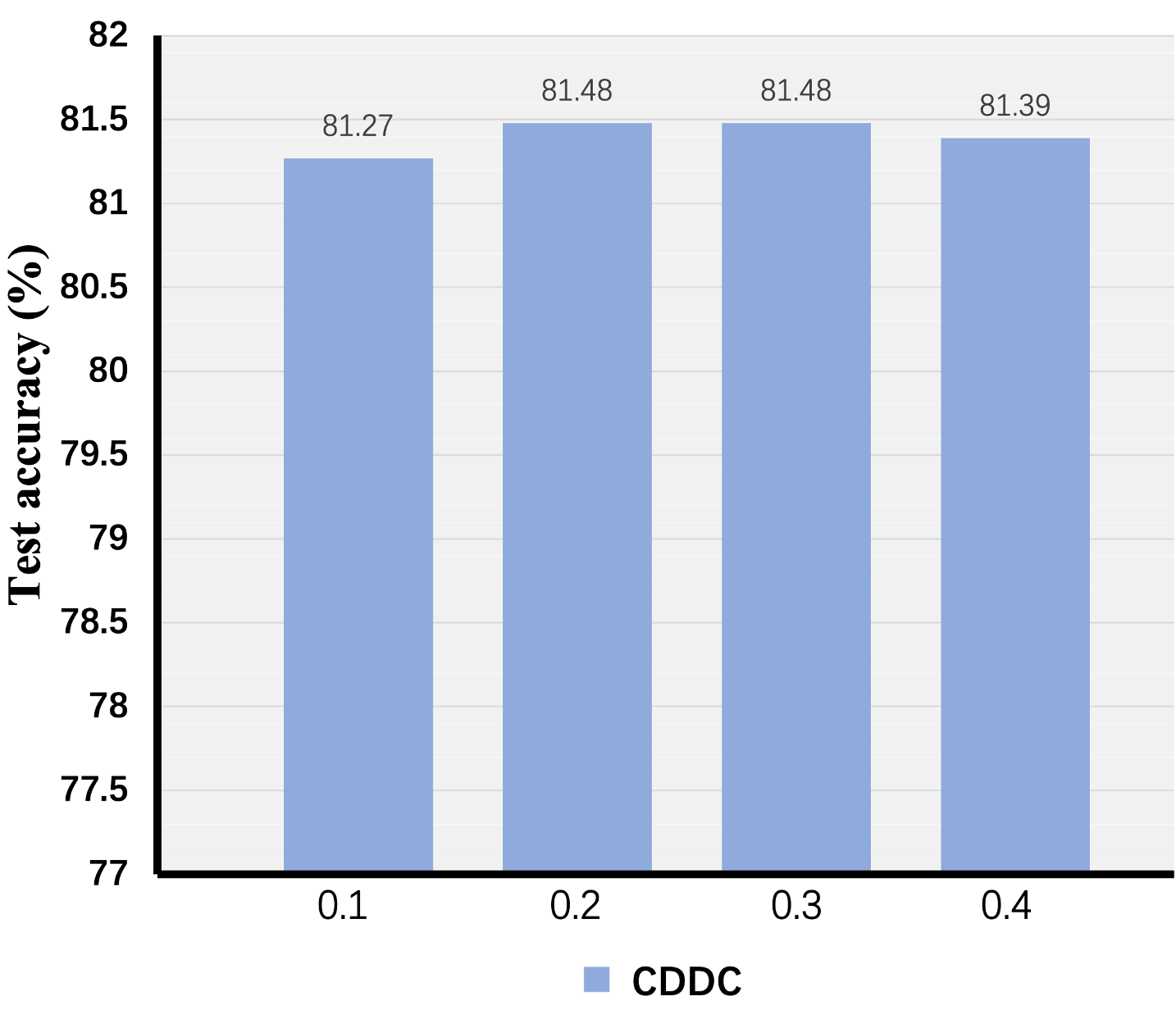
(a) Type-I + 30% Sym. noise

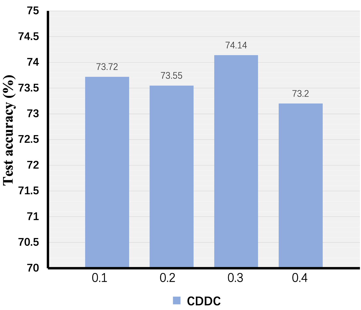
(b) Type-I + 60% Sym. noise

Figure 4. Results of ablation study on noisy CIFAR-1O under different values of $\alpha$.

The influence of $\lambda$. Recall that we sample $\lambda$ proportion data points from the built multivariate Gaussian distributions. Here, Figure 5 shows the influence of $\lambda$ with different values. Specifically, the value of hyperparameter $\lambda$ is chosen in $\{0.10,0.15,0.20,0.25\}$.

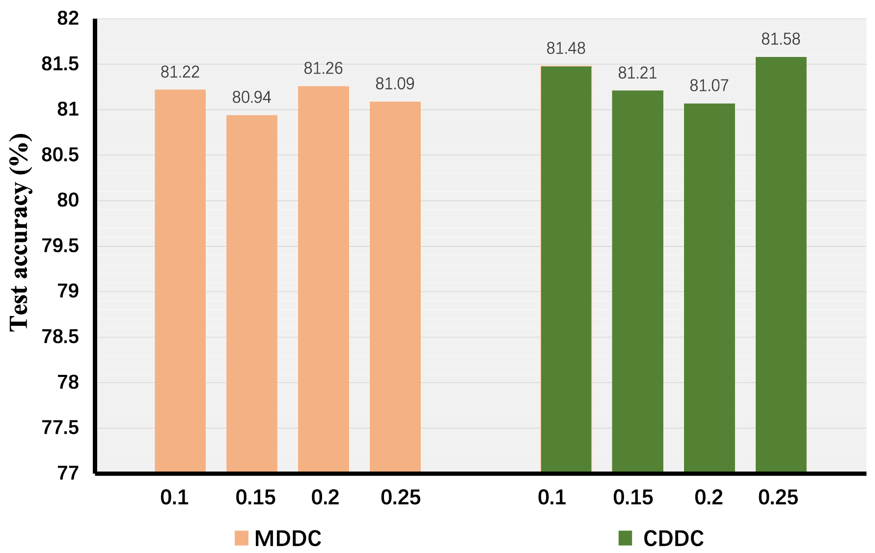
(a) Type-I + 30% Sym. noise

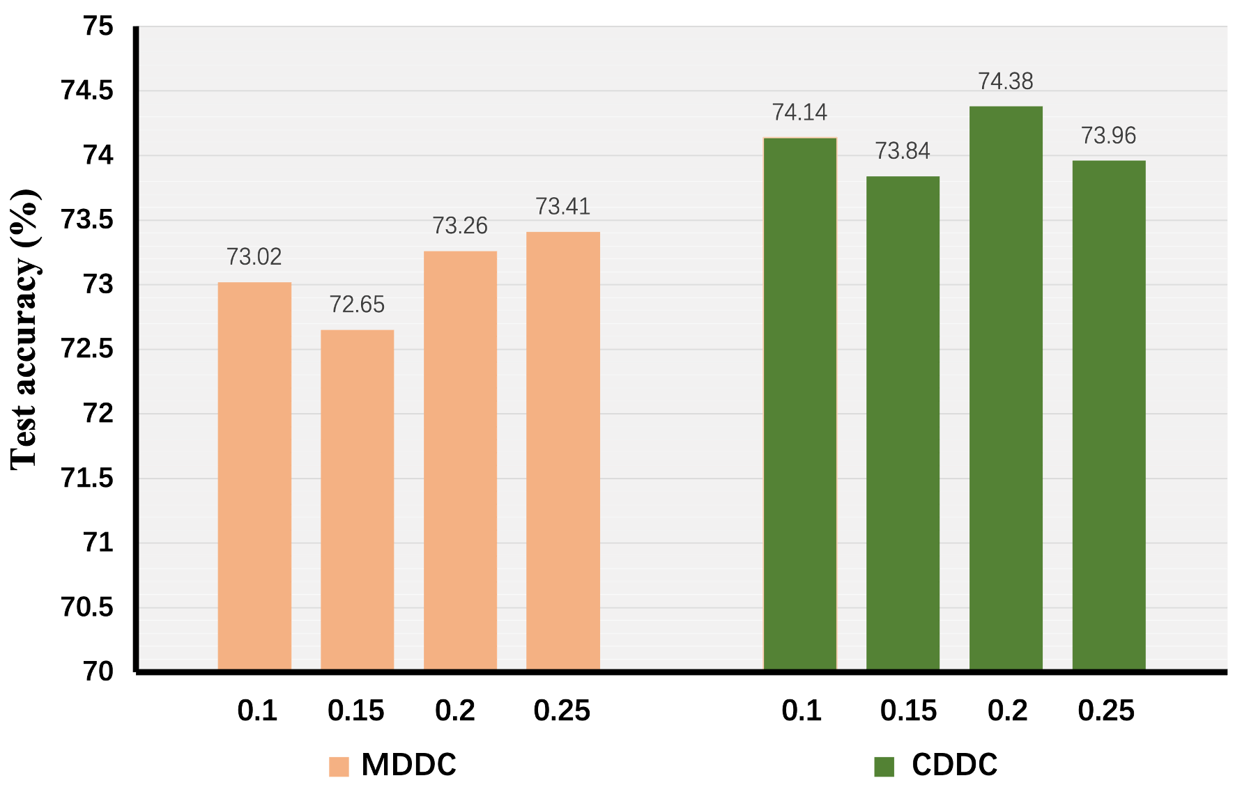
(b) Type-I + 60% Sym. noise

Figure 5. Results of ablation study on noisy CIFAR-1O under differnet values of $\lambda$.

Table 6. Mean and standard deviations of test accuracy (%) on noisy CIFAR-10 with different networks. The improvement of MDDC and CDDC over PLC is highlighted.

Network	Noise	PLC	MDDC	CDDC
SENet18	Type-I+30% Sym.	78.45$\pm$0.43	80.88$\pm$0.22↑2.43	80.35$\pm$0.15↑1.90
	Type-I+60% Sym.	72.56$\pm$0.19	72.65$\pm$0.95↑0.09	72.69$\pm$0.53↑0.13
	Type-I+30% Asym.	77.33$\pm$0.60	78.46 $\pm$1.14↑1.13	78.52$\pm$0.75↑1.19
MobileNetV2	Type-I+30% Sym.	74.90$\pm$0.81	80.49$\pm$0.20↑5.59	80.29$\pm$0.17↑5.39
	Type-I+60% Sym.	71.35$\pm$1.10	72.27$\pm$1.16↑0.92	73.79$\pm$0.96↑2.44
	Type-I+30% Asym.	75.74$\pm$0.82	78.23 $\pm$0.32↑2.58	78.64$\pm$0.34↑2.90
WRN-40-2	Type-I+30% Sym.	72.52$\pm$0.50	79.30$\pm$0.01↑6.78	78.80$\pm$0.41↑6.28
	Type-I+60% Sym.	70.90$\pm$0.03	68.79$\pm$0.09↓2.11	71.41$\pm$0.09↑0.51
	Type-I+30% Asym.	75.01$\pm$0.32	78.08$\pm$0.28↑3.07	77.91$\pm$0.58↑2.90
EfficientNet	Type-I+30% Sym.	71.66$\pm$0.20	78.09$\pm$0.09↑6.43	78.32$\pm$0.04↑6.66
	Type-I+60% Sym.	68.31$\pm$0.14	68.21$\pm$0.69↓0.10	70.58$\pm$0.49↑2.27
	Type-I+30% Asym.	74.11$\pm$0.25	77.83$\pm$0.14↑3.72	77.72$\pm$0.22↑3.61

The results with different networks. Before this, on CIFAR-10 and CIFAR-100, we have shown that our methods are effective with a preact ResNet-34 network. To show our methods are robust to different network structures, we exploit SENet18 (Hu et al., 2018), MobileNetV2 (Howard et al., 2018), WRN-40-2 (Zagoruyko and Komodakis, 2016), and EfficientNet (Tan and Le, 2019). The performance of our methods using these networks is shown in Table 6.

These results show that our methods are not sensitive to the value of $\alpha$ and $\lambda$. Moreover, our methods are robust to the choice of networks. The results imply that it is easy to apply our methods in real-world scenarios.

5. Conclusion

We propose a dynamic distribution-calibration strategy to handle the distribution shift problem brought by instance-dependent label noise. We suppose that before training data are corrupted by label noise, each class conforms to a multivariate Gaussian distribution at the feature level. Afterwards, two methods named MDDC and CDDC are proposed to calibrate the shifted distribution. Extensive experiments show that our methods can help improve the robustness against complicated instance-dependent label noise.

References

- (1)
- Arpit et al. (2017) Devansh Arpit, Stanisław Jastrz\kebski, Nicolas Ballas, David Krueger, Emmanuel Bengio, Maxinder S Kanwal, Tegan Maharaj, Asja Fischer, Aaron Courville, Yoshua Bengio, et al. 2017. A closer look at memorization in deep networks. In ICML. 233–242.
- Berthon et al. (2021) Antonin Berthon, Bo Han, Gang Niu, Tongliang Liu, and Masashi Sugiyama. 2021. Confidence Scores Make Instance-dependent Label-noise learning possible. In ICML.
- Chen et al. (2019) Pengfei Chen, Ben Ben Liao, Guangyong Chen, and Shengyu Zhang. 2019. Understanding and utilizing deep neural networks trained with noisy labels. In ICML. 1062–1070.
- Chen et al. (2020) Pengfei Chen, Junjie Ye, Guangyong Chen, Jingwei Zhao, and Pheng-Ann Heng. 2020. Beyond Class-Conditional Assumption: A Primary Attempt to Combat Instance-Dependent Label Noise. arXiv preprint arXiv:2012.05458 (2020).
- Cheng et al. (2020b) Hao Cheng, Zhaowei Zhu, Xingyu Li, Yifei Gong, Xing Sun, and Yang Liu. 2020b. Learning with instance-dependent label noise: A sample sieve approach. arXiv preprint arXiv:2010.02347 (2020).
- Cheng et al. (2020a) Jiacheng Cheng, Tongliang Liu, Kotagiri Ramamohanarao, and Dacheng Tao. 2020a. Learning with bounded instance-and label-dependent label noise. In ICML.
- Collier et al. (2021) Mark Collier, Basil Mustafa, Efi Kokiopoulou, Rodolphe Jenatton, and Jesse Berent. 2021. Correlated Input-Dependent Label Noise in Large-Scale Image Classification. In Proceedings of the IEEE/CVF Conference on Computer Vision and Pattern Recognition. 1551–1560.
- Diakonikolas and Kane (2019) Ilias Diakonikolas and Daniel M Kane. 2019. Recent advances in algorithmic high-dimensional robust statistics. arXiv preprint arXiv:1911.05911 (2019).
- Feng et al. (2021) Lei Feng, Senlin Shu, Zhuoyi Lin, Fengmao Lv, Li Li, and Bo An. 2021. Can cross entropy loss be robust to label noise?. In IJCAI. 2206–2212.
- Hampel et al. (2011) Frank R Hampel, Elvezio M Ronchetti, Peter J Rousseeuw, and Werner A Stahel. 2011. Robust statistics: the approach based on influence functions. Vol. 196. John Wiley & Sons.
- Han et al. (2020) Bo Han, Gang Niu, Xingrui Yu, Quanming Yao, Miao Xu, Ivor Tsang, and Masashi Sugiyama. 2020. Sigua: Forgetting may make learning with noisy labels more robust. In ICML. 4006–4016.
- Han et al. (2018) Bo Han, Jiangchao Yao, Gang Niu, Mingyuan Zhou, Ivor Tsang, Ya Zhang, and Masashi Sugiyama. 2018. Masking: A new perspective of noisy supervision. In NeurIPS. 5836–5846.
- Hendrycks et al. (2018) Dan Hendrycks, Mantas Mazeika, Duncan Wilson, and Kevin Gimpel. 2018. Using trusted data to train deep networks on labels corrupted by severe noise. In NeurIPS.
- Hernández-Lobato et al. (2014) Daniel Hernández-Lobato, Viktoriia Sharmanska, Kristian Kersting, Christoph H Lampert, and Novi Quadrianto. 2014. Mind the nuisance: Gaussian process classification using privileged noise. In NeurIPS. 837–845.
- Howard et al. (2018) Andrew Howard, Andrey Zhmoginov, Liang-Chieh Chen, Mark Sandler, and Menglong Zhu. 2018. Inverted residuals and linear bottlenecks: Mobile networks for classification, detection and segmentation. (2018).
- Hu et al. (2018) Jie Hu, Li Shen, and Gang Sun. 2018. Squeeze-and-excitation networks. In Proceedings of the IEEE conference on computer vision and pattern recognition. 7132–7141.
- Huang et al. (2019) Jinchi Huang, Lie Qu, Rongfei Jia, and Binqiang Zhao. 2019. O2u-net: A simple noisy label detection approach for deep neural networks. In ICCV. 3326–3334.
- Huber (1992) Peter J Huber. 1992. Robust estimation of a location parameter. In Breakthroughs in statistics. Springer, 492–518.
- Huber (2004) Peter J Huber. 2004. Robust statistics. Vol. 523. John Wiley & Sons.
- Jiang et al. (2022) Zhimeng Jiang, Kaixiong Zhou, Zirui Liu, Li Li, Rui Chen, Soo-Hyun Choi, and Xia Hu. 2022. An Information Fusion Approach to Learning with Instance-Dependent Label Noise. In ICLR.
- Kendall and Gal (2017) Alex Kendall and Yarin Gal. 2017. What uncertainties do we need in bayesian deep learning for computer vision?. In NeurIPS.
- Kim et al. (2021) Taehyeon Kim, Jongwoo Ko, JinHwan Choi, Se-Young Yun, et al. 2021. FINE Samples for Learning with Noisy Labels. In NeurIPS.
- Kim et al. (2019) Youngdong Kim, Junho Yim, Juseung Yun, and Junmo Kim. 2019. Nlnl: Negative learning for noisy labels. In ICCV. 101–110.
- Kingma et al. (2016) Durk P Kingma, Tim Salimans, Rafal Jozefowicz, Xi Chen, Ilya Sutskever, and Max Welling. 2016. Improved variational inference with inverse autoregressive flow. In NeurIPS.
- Kingma and Welling (2013) Diederik P Kingma and Max Welling. 2013. Auto-encoding variational bayes. arXiv preprint arXiv:1312.6114 (2013).
- Krizhevsky (2009) Alex Krizhevsky. 2009. Learning multiple layers of features from tiny images. Technical Report.
- Lai et al. (2016) Kevin A Lai, Anup B Rao, and Santosh Vempala. 2016. Agnostic estimation of mean and covariance. In 2016 IEEE 57th Annual Symposium on Foundations of Computer Science (FOCS). IEEE, 665–674.
- Lee et al. (2019) Kimin Lee, Sukmin Yun, Kibok Lee, Honglak Lee, Bo Li, and Jinwoo Shin. 2019. Robust inference via generative classifiers for handling noisy labels. In ICML. 3763–3772.
- Lee et al. (2018) Kuang-Huei Lee, Xiaodong He, Lei Zhang, and Linjun Yang. 2018. Cleannet: Transfer learning for scalable image classifier training with label noise. In CVPR. 5447–5456.
- Li et al. (2020) Junnan Li, Richard Socher, and Steven C.H. Hoi. 2020. DivideMix: Learning with Noisy Labels as Semi-supervised Learning. In ICLR.
- Li et al. (2022) Xiaotong Li, Yongxing Dai, Yixiao Ge, Jun Liu, Ying Shan, and Ling-Yu Duan. 2022. Uncertainty Modeling for Out-of-Distribution Generalization. arXiv preprint arXiv:2202.03958 (2022).
- Li et al. (2021) Xuefeng Li, Tongliang Liu, Bo Han, Gang Niu, and Masashi Sugiyama. 2021. Provably End-to-end Label-Noise Learning without Anchor Points. In ICML.
- Li et al. (2017) Yuncheng Li, Jianchao Yang, Yale Song, Liangliang Cao, Jiebo Luo, and Li-Jia Li. 2017. Learning from noisy labels with distillation. In ICCV. 1910–1918.
- Liu et al. (2020) Sheng Liu, Jonathan Niles-Weed, Narges Razavian, and Carlos Fernandez-Granda. 2020. Early-learning regularization prevents memorization of noisy labels. In NeurIPS.
- Liu and Guo (2019) Yang Liu and Hongyi Guo. 2019. Peer Loss Functions: Learning from Noisy Labels without Knowing Noise Rates. arXiv preprint arXiv:1910.03231 (2019).
- Lukasik et al. (2020) Michal Lukasik, Srinadh Bhojanapalli, Aditya Menon, and Sanjiv Kumar. 2020. Does label smoothing mitigate label noise?. In ICML. 6448–6458.
- Lyu and Tsang (2020) Yueming Lyu and Ivor W. Tsang. 2020. Curriculum Loss: Robust Learning and Generalization against Label Corruption. In ICLR.
- Ma et al. (2020) Xingjun Ma, Hanxun Huang, Yisen Wang, Simone Romano, Sarah Erfani, and James Bailey. 2020. Normalized loss functions for deep learning with noisy labels. In ICML. 6543–6553.
- Mohri et al. (2018) Mehryar Mohri, Afshin Rostamizadeh, and Ameet Talwalkar. 2018. Foundations of Machine Learning. MIT Press.
- Nguyen et al. (2020) Duc Tam Nguyen, Chaithanya Kumar Mummadi, Thi Phuong Nhung Ngo, Thi Hoai Phuong Nguyen, Laura Beggel, and Thomas Brox. 2020. SELF: Learning to Filter Noisy Labels with Self-Ensembling. In ICLR.
- Nishi et al. (2021) Kento Nishi, Yi Ding, Alex Rich, and Tobias Hollerer. 2021. Augmentation strategies for learning with noisy labels. In CVPR. 8022–8031.
- Northcutt et al. (2021) Curtis Northcutt, Lu Jiang, and Isaac Chuang. 2021. Confident learning: Estimating uncertainty in dataset labels. Journal of Artificial Intelligence Research 70 (2021), 1373–1411.
- Ortego et al. (2021) Diego Ortego, Eric Arazo, Paul Albert, Noel E O’Connor, and Kevin McGuinness. 2021. Multi-objective interpolation training for robustness to label noise. In CVPR. 6606–6615.
- Patrini et al. (2017) Giorgio Patrini, Alessandro Rozza, Aditya Krishna Menon, Richard Nock, and Lizhen Qu. 2017. Making deep neural networks robust to label noise: A loss correction approach. In CVPR. 1944–1952.
- Pleiss et al. (2020) Geoff Pleiss, Tianyi Zhang, Ethan R Elenberg, and Kilian Q Weinberger. 2020. Identifying mislabeled data using the area under the margin ranking. In NeurIPS.
- Sachdeva et al. (2021) Ragav Sachdeva, Filipe R Cordeiro, Vasileios Belagiannis, Ian Reid, and Gustavo Carneiro. 2021. Evidentialmix: Learning with combined open-set and closed-set noisy labels. In WACV. 3607–3615.
- Seo et al. (2019) Paul Hongsuck Seo, Geeho Kim, and Bohyung Han. 2019. Combinatorial inference against label noise. In NeurIPS. 1173–1183.
- Sugiyama and Kawanabe (2012) Masashi Sugiyama and Motoaki Kawanabe. 2012. Machine learning in non-stationary environments: Introduction to covariate shift adaptation. MIT press.
- Szegedy et al. (2017) Christian Szegedy, Sergey Ioffe, Vincent Vanhoucke, and Alexander A Alemi. 2017. Inception-v4, inception-resnet and the impact of residual connections on learning. In AAAI.
- Tan et al. (2021) Cheng Tan, Jun Xia, Lirong Wu, and Stan Z Li. 2021. Co-learning: Learning from noisy labels with self-supervision. In ACM MM. 1405–1413.
- Tan and Le (2019) Mingxing Tan and Quoc Le. 2019. Efficientnet: Rethinking model scaling for convolutional neural networks. In International conference on machine learning. PMLR, 6105–6114.
- Tanaka et al. (2018) Daiki Tanaka, Daiki Ikami, Toshihiko Yamasaki, and Kiyoharu Aizawa. 2018. Joint Optimization Framework for Learning with Noisy Labels. In CVPR.
- Thekumparampil et al. (2018) Kiran K Thekumparampil, Ashish Khetan, Zinan Lin, and Sewoong Oh. 2018. Robustness of conditional GANs to noisy labels. In NeurIPS. 10271–10282.
- Wang et al. (2019a) Yisen Wang, Xingjun Ma, Zaiyi Chen, Yuan Luo, Jinfeng Yi, and James Bailey. 2019a. Symmetric cross entropy for robust learning with noisy labels. In Proceedings of the IEEE/CVF International Conference on Computer Vision. 322–330.
- Wang et al. (2019b) Yulin Wang, Xuran Pan, Shiji Song, Hong Zhang, Gao Huang, and Cheng Wu. 2019b. Implicit semantic data augmentation for deep networks. Advances in Neural Information Processing Systems 32 (2019).
- Wei et al. (2020) Hongxin Wei, Lei Feng, Xiangyu Chen, and Bo An. 2020. Combating noisy labels by agreement: A joint training method with co-regularization. In CVPR. 13726–13735.
- Wei and Liu (2021) Jiaheng Wei and Yang Liu. 2021. When Optimizing -divergence is Robust with Label Noise. In ICLR.
- Wu et al. (2021b) Songhua Wu, Xiaobo Xia, Tongliang Liu, Bo Han, Mingming Gong, Nannan Wang, Haifeng Liu, and Gang Niu. 2021b. Class2Simi: A Noise Reduction Perspective on Learning with Noisy Labels. In ICML.
- Wu et al. (2021a) Zhi-Fan Wu, Tong Wei, Jianwen Jiang, Chaojie Mao, Mingqian Tang, and Yu-Feng Li. 2021a. Ngc: A unified framework for learning with open-world noisy data. In ICCV. 62–71.
- Xia et al. (2022a) Xiaobo Xia, Bo Han, Nannan Wang, Jiankang Deng, Jiatong Li, Yinian Mao, and Tongliang Liu. 2022a. Extended T: Learning with Mixed Closed-set and Open-set Noisy Labels. IEEE Transactions on Pattern Analysis and Machine Intelligence (2022).
- Xia et al. (2021) Xiaobo Xia, Tongliang Liu, Bo Han, Chen Gong, Nannan Wang, Zongyuan Ge, and Yi Chang. 2021. Robust early-learning: Hindering the memorization of noisy labels. In ICLR.
- Xia et al. (2022b) Xiaobo Xia, Tongliang Liu, Bo Han, Mingming Gong, Jun Yu, Gang Niu, and Masashi Sugiyama. 2022b. Sample Selection with Uncertainty of Losses for Learning with Noisy Labels. In ICLR.
- Xia et al. (2020) Xiaobo Xia, Tongliang Liu, Bo Han, Nannan Wang, Mingming Gong, Haifeng Liu, Gang Niu, Dacheng Tao, and Masashi Sugiyama. 2020. Part-dependent label noise: Towards instance-dependent label noise. In NeurIPS.
- Xia et al. (2019) Xiaobo Xia, Tongliang Liu, Nannan Wang, Bo Han, Chen Gong, Gang Niu, and Masashi Sugiyama. 2019. Are Anchor Points Really Indispensable in Label-Noise Learning?. In NeurIPS. 6835–6846.
- Xiao et al. (2015) Tong Xiao, Tian Xia, Yi Yang, Chang Huang, and Xiaogang Wang. 2015. Learning from massive noisy labeled data for image classification. In CVPR. 2691–2699.
- Yang et al. (2021) Shuo Yang, Lu Liu, and Min Xu. 2021. Free Lunch for Few-shot Learning: Distribution Calibration. In ICLR.
- Yao et al. (2020) Quanming Yao, Hansi Yang, Bo Han, Gang Niu, and James Tin-Yau Kwok. 2020. Searching to exploit memorization effect in learning with noisy labels. In ICML. 10789–10798.
- Yao et al. (2021) Yazhou Yao, Zeren Sun, Chuanyi Zhang, Fumin Shen, Qi Wu, Jian Zhang, and Zhenmin Tang. 2021. Jo-src: A contrastive approach for combating noisy labels. In CVPR. 5192–5201.
- Yi and Wu (2019) Kun Yi and Jianxin Wu. 2019. Probabilistic end-to-end noise correction for learning with noisy labels. In CVPR. 7017–7025.
- Yu et al. (2019) Xingrui Yu, Bo Han, Jiangchao Yao, Gang Niu, Ivor W Tsang, and Masashi Sugiyama. 2019. How Does Disagreement Benefit Co-teaching?. In ICML.
- Zagoruyko and Komodakis (2016) Sergey Zagoruyko and Nikos Komodakis. 2016. Wide residual networks. arXiv preprint arXiv:1605.07146 (2016).
- Zhang et al. (2021a) Yivan Zhang, Gang Niu, and Masashi Sugiyama. 2021a. Learning Noise Transition Matrix from Only Noisy Labels via Total Variation Regularization. In ICML.
- Zhang et al. (2021b) Yikai Zhang, Songzhu Zheng, Pengxiang Wu, Mayank Goswami, and Chao Chen. 2021b. Learning with Feature-Dependent Label Noise: A Progressive Approach. In ICLR.
- Zhang and Sabuncu (2018) Zhilu Zhang and Mert Sabuncu. 2018. Generalized cross entropy loss for training deep neural networks with noisy labels. In NeurIPS. 8778–8788.
- Zheng et al. (2020) Songzhu Zheng, Pengxiang Wu, Aman Goswami, Mayank Goswami, Dimitris Metaxas, and Chao Chen. 2020. Error-bounded correction of noisy labels. In ICML. 11447–11457.
- Zhu et al. (2021) Zhaowei Zhu, Tongliang Liu, and Yang Liu. 2021. A second-order approach to learning with instance-dependent label noise. In CVPR. 10113–10123.