Distributed-Memory Randomized Algorithms for Sparse Tensor CP Decomposition

Abstract

Sparse Candecomp / PARAFAC decomposition, a generalization of the matrix singular value decomposition to higher-dimensional tensors, is a popular tool for analyzing diverse datasets. On tensors with billions of nonzero entries, computing a CP decomposition is a computationally intensive task. We propose the first distributed-memory implementations of two randomized CP decomposition algorithms, CP-ARLS-LEV and STS-CP, that offer nearly an order-of-magnitude speedup at high decomposition ranks over well-tuned non-randomized decomposition packages. Both algorithms rely on leverage score sampling and enjoy strong theoretical guarantees, each with varying time and accuracy tradeoffs. We tailor the communication schedule for our random sampling algorithms, eliminating expensive reduction collectives and forcing communication costs to scale with the random sample count. Finally, we optimize the local storage format for our methods, switching between an analogue of compressed sparse column and compressed sparse row formats to facilitate both random sampling and efficient parallelization of sparse-dense matrix multiplication. Experiments show that our methods are fast and scalable, producing 11x speedup over SPLATT to compute a decomposition of the billion-scale Reddit tensor on 512 CPU cores in under 2 minutes.

I Introduction

Randomized algorithms for numerical linear algebra have become increasingly popular in the past decade, but their distributed-memory communication characteristics and scaling properties have received less attention. In this work, we examine randomized algorithms to compute the Candecomp / PARAFAC (CP) decomposition, a generalization of the matrix singular-value decomposition to dimensions higher than 2. Given a tensor $\mathcal{T}\in\mathbb{R}^{I_{1}\times...\times I_{N}}$ and a target rank $R$, the goal of CP decomposition is to find a set of factor matrices $U_{1},...,U_{N},U_{j}\in\mathbb{R}^{I_{j}\times R}$ with unit norm columns and a nonnegative vector $\sigma\in\mathbb{R}^{R}$ satisfying

$$\mathcal{T}\left[i_{1},...,i_{N}\right]\approx\sum_{r=1}^{R}\sigma\left[r\right]U_{1}\left[i_{1},r\right]...U_{N}\left[i_{N},r\right].$$ (1)

We consider real sparse tensors $\mathcal{T}$ with $N\geq 3$ (each dimension is called a “mode”), all entries known, and billions of nonzero entries. Sparse tensors are a flexible abstraction for a variety of data, such as network traffic logs [1], text corpora [2], and knowledge graphs [3]. Computing the CP decomposition of a sparse tensor can be interpreted as learning a dense embedding vector for every index $i_{j}\in I_{j}$ for $1\leq j\leq N$. These embeddings have been used to mine patterns from social networks [4], detect anomalies in packet traces [1], and monitor trends in internal network traffic [5].

One of the most popular methods for computing the CP decomposition, the Alternating-Least-Squares (ALS) algorithm, involves repeatedly solving large, overdetermined linear least-squares problems with structured design matrices [6]. High-performance libraries DFacto[7], SPLATT [8], HyperTensor [9], and BigTensor [10] distribute these expensive computations to a cluster of processors that communicate through an interconnect. Separately, several works use randomized sampling methods to accelerate the least-squares solves, with prototypes implemented in a shared-memory setting [11, 4, 12, 13]. These randomized algorithms have strong theoretical guarantees and offer significant asymptotic advantages over non-randomized ALS. Unfortunately, prototypes of these methods require hours to run [4, 13] and are neither competitive nor scalable compared to existing libraries with distributed-memory parallelism.

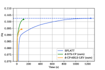
Figure 1: Running maximum accuracy over time for SPLATT, a state-of-the-art distributed CP decomposition software package, and our randomized algorithms on the Reddit tensor, target rank $R=100$, on 512 CPU cores across 4 nodes. Curves are averages of 5 trials, 80 ALS rounds.

We extend two randomized decomposition algorithms, CP-ARLS-LEV [4] and STS-CP [13], to the distributed-memory parallel setting and provide high-performance implementations to handle massive datasets. These are the first implementations of these algorithms that scale to thousands of CPU cores. To address the unique challenges that randomized algorithms pose in a parallel setting, we introduce several key innovations, three of which we highlight:

• Choice of Sampling Algorithms: We distribute two distinct randomized methods that downsample the design matrix and sparse tensor in each linear least-squares problem. The first, CP-ARLS-LEV, requires minimal computation and communication overhead, but may suffer from accuracy loss for high ranks and large tensors. The second, STS-CP, has asymptotically higher communication and computation costs, but produces decompositions of higher final accuracy for the same sample count. We show that either of these algorithms may be appropriate depending on the speedup / accuracy desired.

• Communication Costs and Load Balance: We demonstrate that communication-optimal schedules for non-randomized ALS may exhibit disproportionately high communication costs for randomized algorithms. To combat this, we use an “accumulator-stationary” schedule that eliminates expensive Reduce-scatter collectives, causing all communication costs to scale with the number of random samples taken. This alternate schedule may significantly reduce communication costs on tensors with large dimensions (Figure 7) and empirically improves the computational load balance (Figure 10).

• Local Tensor Storage Format: We use a modified compressed-sparse-column format to store each matricization of our tensor, allowing efficient selection of nonzero entries by our random sampling algorithms. We then transform the selected nonzero entries into compressed sparse row format, which eliminates shared-memory data races in the subsequent sparse-dense matrix multiplication. We observe that the cost of the transposition is justified and provides a roughly 1.7x speedup over using atomics in a hybrid OpenMP / MPI implementation.

On hundreds to thousands of CPU cores, our distributed-memory randomized algorithms have significant advantages over non-randomized CP decomposition libraries while preserving the accuracy of the final approximation. As Figure 1 shows, our method d-STS-CP computes a rank 100 decomposition of the Reddit tensor ($\sim 4.7$ billion nonzero entries) with a 11x speedup over SPLATT, a state-of-the-art distributed-memory CP decomposition package. The reported speedup was achieved on 512 CPU cores, with a final fit within $0.8\%$ of non-randomized ALS for the same iteration count. While the distributed algorithm d-CP-ARLS-LEV achieves a lower final accuracy, it makes progress faster than SPLATT and spends less time on sampling (completing 80 rounds in an average of 81 seconds). We demonstrate that it is well-suited to smaller tensors and lower target ranks.

Figure 2: Top: the linear least-squares problem to optimize factor matrix $U_{2}$ during the ALS algorithm for a 3D tensor (column dimension of $\textrm{mat}(\mathcal{T},2)$ not to scale). Middle: the exact solution to the problem using the Matricized Tensor Times Khatri-Rao Product (MTTKRP). Shaded columns of $\textrm{mat}(\mathcal{T},2)$ and rows of $(U_{3}\odot U_{1})$ are selected by our random sampling algorithm. Bottom: the downsampled linear least-squares problem after applying the random sampling matrix $S$ to decrease computation costs.

II Notation and Preliminaries

Symbol	Description
$\mathcal{T}$	Sparse tensor of dimensions $I_{1}\times\ldots\times I_{N}$
$R$	Target Rank of CP Decomposition
$U_{1},\ldots,U_{N}$	Dense factor matrices, $U_{j}\in\mathbb{R}^{I_{j}\times R}$
$\sigma$	Vector of scaling factors, $\sigma\in\mathbb{R}^{R}$
$J$	Sample count for randomized ALS
$\cdot$	Matrix multiplication
$\circledast$	Elementwise multiplication
$\otimes$	Kronecker product
$\odot$	Khatri-Rao product
$P$	Total processor count
$P_{1},\ldots,P_{N}$	Dimensions of processor grid, $\prod_{i}P_{i}=P$
$U_{i}^{(p_{j})}$	Block row of $U_{i}$ owned by processor $p_{j}$

TABLE I: Symbol Definitions

Table I summarizes our notation. We use script characters (e.g. $\mathcal{T}$) to denote tensors with at least three modes, capital letters for matrices, and lowercase letters for vectors. Bracketed tuples following any of these objects, e.g. $A\left[i,j\right]$, represent indexes into each object, and the symbol “:” in place of any index indicates a slicing of a tensor. We use $\odot$ to denote the Khatri-Rao product, which is a column-wise Kronecker product of a pair of matrices with the same number of columns. For $A\in\mathbb{R}^{I\times R},B\in\mathbb{R}^{J\times R}$, $A\odot B$ produces a matrix of dimensions $(IJ)\times R$ such that for $1\leq j\leq R$,

$$(A\odot B)\left[:,j\right]=A\left[:,j\right]\otimes B\left[:,j\right].$$

Let $\mathcal{T}$ be an $N$-dimensional tensor indexed by tuples $(i_{1},...,i_{N})\in\left[I_{1}\right]\times...\times\left[I_{N}\right]$, with $\textrm{nnz}(\mathcal{T})$ as the number of nonzero entries. In this work, sparse tensors are always represented as a collection of $(N+1)$-tuples, with the first $N$ elements giving the indices of a nonzero element and the last element giving the value. We seek a low-rank approximation of $\mathcal{T}$ given by Equation (1), the right-hand-side of which we abbreviate as $\left[\sigma;U_{1},...,U_{N}\right]$. By convention, each column of $U_{1},...,U_{N}$ has unit norm. Our goal is to minimize the sum of squared differences between our approximation and the provided tensor:

$$\textrm{argmin}_{\sigma,U_{1},\ldots,U_{N}}\left\lVert\left[\sigma;U_{1},...,U_{N}\right]-\mathcal{T}\right\rVert_{\textrm{F}}^{2}.$$ (2)

II-A CP Decomposition via Non-Randomized ALS

Minimizing Equation (2) jointly over $U_{1},...,U_{N}$ is still a non-convex problem (the vector $\sigma$ can be computed directly from the factor matrices by renormalizing each column). Alternating least squares is a popular heuristic algorithm that iteratively drives down the approximation error. The algorithm begins with a set of random factor matrices and optimizes the approximation in rounds, each involving $N$ subproblems. The $j$-th subproblem in a round holds all factor matrices but $U_{j}$ constant and solves for a new matrix $\hat{U}_{j}$ minimizing the squared Frobenius norm error [6]. The updated matrix $\hat{U}_{j}$ is the solution to the overdetermined linear least-squares problem

$$\hat{U}_{j}:=\min_{X}\left\lVert U_{\neq j}\cdot X^{\top}-\textrm{mat}(\mathcal{T},j)^{\top}\right\rVert_{F}.$$ (3)

Here, the design matrix is

$$U_{\neq j}:=U_{N}\odot...\odot U_{j+1}\odot U_{j-1}\odot...\odot U_{1},$$

which is a Khatri-Rao Product (KRP) of the factors held constant. The matrix $\textrm{mat}(\mathcal{T},j)$ is a matricization of the sparse tensor $\mathcal{T}$, which reorders the tensor modes and flattens it into a matrix of dimensions $I_{j}\times(\prod_{i\neq j}I_{i})$. We solve the problem efficiently using the normal equations. Denoting the Gram matrix by $G=(U_{\neq j})^{\top}(U_{\neq j})$, we have

$$\hat{U}_{j}:=\textrm{mat}(\mathcal{T},j)\cdot U_{\neq j}\cdot G^{+},$$ (4)

where $G^{+}$ is the Moore-Penrose pseudo-inverse of $G$. Since $U_{\neq j}$ is a Khatri-Rao product, we can efficiently compute $G$ through the well-known [6] formula

$$G=\operatorname*{\scalerel*{\circledast}{\sum}}_{k\neq j}(U_{k}^{\top}U_{k}),$$ (5)

where $\circledast$ denotes elementwise multiplication. Figure 2 illustrates each least-squares problem, and Algorithm 1 summarizes the ALS procedure, including a renormalization of factor matrix columns after each solve. We implement the initialization step in line 1 by drawing all factor matrix entries from a unit-variance Gaussian distribution, a standard technique [4].

Algorithm 1 CP-ALS($\mathcal{T}$, $R$)

1:  Initialize $U_{j}\in\mathbb{R}^{I_{j}\times R}$ randomly for $1\leq j\leq N$.

2:  Renorm. $U_{j}\left[:,i\right]\mathrel{/}=\left\lVert U_{j}\left[:,i\right]\right\rVert_{2}$, $1\leq j\leq N,1\leq i\leq R$.

3:  Initialize $\sigma\in\mathbb{R}^{R}$ to $\left[1\right]$.

4:  while not converged do

5:     for $j=1...N$ do

6:        $U_{j}:=\textrm{argmin}_{X}\left\lVert U_{\neq j}\cdot X^{\top}-\textrm{mat}(\mathcal{T},j)^{\top}\right\rVert_{F}$

7:        $\sigma\left[i\right]=\left\lVert U_{j}\left[:,i\right]\right\rVert_{2}$, $1\leq i\leq R$

8:        Renorm. $U_{j}\left[:,i\right]\mathrel{/}=\left\lVert U_{j}\left[:,i\right]\right\rVert_{2}$, $1\leq i\leq R$.

9:  return $\left[\sigma;U_{1},...,U_{N}\right]$.

The most expensive component of the ALS algorithm is the matrix multiplication $\textrm{mat}(\mathcal{T},j)\cdot U_{\neq j}$ in Equation (4), an operation known as the Matricized Tensor-Times-Khatri Rao Product (MTTKRP). For a sparse tensor $\mathcal{T}$, this kernel has a computational pattern similar to sparse-dense matrix multiplication (SpMM): for each nonzero in the sparse tensor, we compute a scaled Hadamard product between $N-1$ rows of the constant factor matrices and add it to a row of the remaining factor matrix. The MTTKRP runtime is

$$O(\textrm{nnz}(\mathcal{T})NR),$$ (6)

which is linear in the nonzero count of $\mathcal{T}$. Because $\mathcal{T}$ may have billions of nonzero entries, we seek methods to drive down the cost of the MTTKRP.

II-B Randomized Leverage Score Sampling

Sketching is a powerful tool to accelerate least squares problems of the form $\min_{X}\|AX-B\|_{\text{F}}$ where $A$ has far more rows than columns [14, 15, 16]. We apply a structured sketching matrix $S^{J\times I}$ to both $A$ and $B$, where the row count of $S$ satisfies $J\ll I$. The resulting problem $\min_{\tilde{X}}\|S(A\tilde{X}-B)\|_{F}$ is cheaper to solve, and the solution $\tilde{X}$ has residual arbitrarily close (for sufficiently high $J$) to the true minimum with high probability. We seek a sketching operator $S$ with an efficiently computable action on $A$, which is a Khatri-Rao product.

We choose $S$ to be a sampling matrix with a single nonzero per row (see Section III-B for alternatives). This matrix extracts and reweights $J$ rows from both $A$ and $B$, preserving the sparsity of the matricized tensor. The cost to solve the $j$-th sketched subproblem is dominated by the downsampled MTTKRP operation $\textrm{mat}(\mathcal{T},j)S^{\top}SU_{\neq j}$, which has runtime

$$O\left(\textrm{nnz}(\textrm{mat}(\mathcal{T},j)S^{\top})NR\right).$$ (7)

As Figure 2 (bottom) illustrates, $\textrm{mat}(\mathcal{T},j)S^{\top}$ typically has far fewer nonzeros than $\mathcal{T}$, enabling sampling to reduce the computation cost in Equation (6). To select indices to sample, we implement two algorithms that involve the leverage scores of the design matrix [11, 4, 13]. Given a matrix $A\in\mathbb{R}^{I\times R}$, the leverage score of row $i$ is given by

$$\ell_{i}=A\left[i,:\right](A^{\top}A)^{+}A\left[i,:\right]^{\top}.$$ (8)

These scores induce a probability distribution over the rows of matrix $A$, which we can interpret as a measure of importance. As the following theorem from Larsen and Kolda [4] (building on similar results by Mahoney and Drineas [15]) shows, sampling from either the exact or approximate distribution of statistical leverage guarantees, with high probability, that the solution to the downsampled problem has low residual with respect to the original problem.

Theorem II.1 (Larsen and Kolda [4]).

Let $S\in\mathbb{R}^{J\times I}$ be a sampling matrix for $A\in\mathbb{R}^{I\times R}$ where each row $i$ is sampled i.i.d. with probability $p_{i}$. Let $\beta=\min_{i\in\left[I\right]}(p_{i}R/\ell_{i})$. For a constant $C$ and any $\varepsilon,\delta\in(0,1)$, let the sample count be

$$J=\frac{R}{\beta}\max\left(C\log\frac{R}{\delta},\frac{1}{\varepsilon\delta}\right).$$

Letting $\tilde{X}=\textrm{argmin}_{\tilde{X}}\left\lVert SA\tilde{X}-SB\right\rVert_{F}$, we have

$$\left\lVert A\tilde{X}-B\right\rVert^{2}_{F}\leq(1+\varepsilon)\min_{X}\left\lVert AX-B\right\rVert_{F}^{2}.$$

with probability at least $1-\delta$.

Here, $\beta\leq 1$ quantifies deviation of the sampling probabilities from the exact leverage score distribution, with a higher sample count $J$ required as the deviation increases. The STS-CP samples from the exact leverage distribution with $\beta=1$, achieving higher accuracy at the expense of increased sampling time. CP-ARLS-LEV samples from an approximate distribution with $\beta<1$.

III Related Work

III-A High-Performance ALS CP Decomposition

Significant effort has been devoted to optimizing the shared-memory MTTKRP using new data structures for the sparse tensor, cache-blocked computation, loop reordering strategies, and methods that minimize data races between threads [17, 18, 19, 20, 21, 22]. Likewise, several works provide high-performance algorithms for ALS CP decomposition in a distributed-memory setting. Smith and Karypis provide an algorithm that distributes load-balanced chunks of the sparse tensor to processors in an $N$-dimensional Cartesian topology [23]. Factor matrices are shared among slices of the topology that require them, and each processor computes a local MTTKRP before reducing results with a subset of processors. The SPLATT library [8] implements this communication strategy and uses the compressed sparse fiber (CSF) format to accelerate local sparse MTTKRP computations on each processor.

Ballard et al. [24]. use a similar communication strategy to compute the MTTKRP involved in dense nonnegative CP decomposition. They further introduce a dimension-tree algorithm that reuses partially computed terms of the MTTKRP between ALS optimization problems. DFacTo [7] instead reformulates the MTTKRP as a sequence of sparse matrix-vector products (SpMV), taking advantage of extensive research optimizing the SpMV kernel. Smith and Karypis [23] note, however, that DFacTo exhibits significant communication overhead. Furthermore, the sequence of SpMV operations cannot take advantage of access locality within rows of the dense factor matrices, leading to more cache misses than strategies based on sparse-matrix-times-dense-matrix-multiplication (SpMM). GigaTensor [25] uses the MapReduce model in Hadoop to scale to distributed, fault-tolerant clusters. Ma and Solomonik [26] use pairwise perturbation to accelerate CP-ALS, reducing the cost of MTTKRP computations when ALS is sufficiently close to convergence using information from prior rounds.

Our work investigates variants of the Cartesian data distribution scheme adapted for a downsampled MTTKRP. We face challenges adapting either specialized data structures for the sparse tensor or dimension-tree algorithms. By extracting arbitrary nonzero elements from the sparse tensor, randomized sampling destroys the advantage conferred by formats such as CSF. Further, each least-squares solve requires a fresh set of rows drawn from the Khatri-Rao product design matrix, which prevents efficient reuse of results from prior MTTKRP computations.

Libraries such as the Cyclops Tensor Framework (CTF) [27] automatically parallelize distributed-memory contractions of both sparse and dense tensors. SpDISTAL [28] proposes a flexible domain-specific language to schedule sparse tensor linear algebra on a cluster, including the MTTKRP operation. The randomized algorithms investigated here could be implemented on top of either library, but it is unlikely that current tensor algebra compilers could automatically produce the optimizations and communication schedules that we propose.

III-B Alternate Methods to Sketch the Khatri-Rao Product

Besides leverage score sampling, popular options for sketching Khatri-Rao products include Fast Fourier Transform-based sampling matrices [29] and structured random sparse matrices (e.g. Countsketch) [30, 31]. The former method, however, introduces fill-in when applied to the sparse matricized tensor $\textrm{mat}(\mathcal{T},j)$. Because the runtime of the downsampled MTTKRP is linearly proportional to the nonzero count of $\textrm{mat}(\mathcal{T},j)S^{\top}$, the advantages of sketching are lost due to fill-in. While Countsketch operators do not introduce fill, they still require access to all nonzeros of the sparse tensor at every iteration, which is expensive when $\textrm{nnz}(\mathcal{T})$ ranges from hundreds of millions to billions.

III-C Alternative Tensor Decomposition Algorithms

Some other algorithms besides ALS exist for large sparse tensor decomposition. Stochastic gradient descent (SGD, investigated by Kolda and Hong [32]) iteratively improves CP factor matrices by sampling minibatches of indices from $\mathcal{T}$, computing the gradient of a loss function at those indices with respect to the factor matrices, and adding a step in the direction of the gradient to the factors. Gradient methods are flexible enough to minimize a variety of loss functions, but require tuning of additional parameters (batch size, learning rate) as well as a distinct parallelization strategy. The CCD++ algorithm [33] extended to tensors keeps all but one rank-1 component of the decomposition fixed and optimizes for the remaining component, in contrast to ALS which keeps all but one factor matrix fixed.

IV Distributed-Randomized CP Decomposition

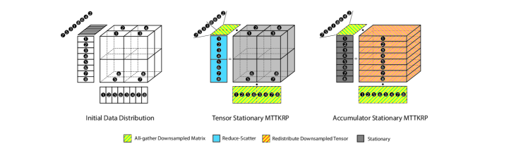
Figure 3: Initial data distribution and downsampled MTTKRP data movement for a 3D tensor, $P=8$ processors. Rectangles along each side of the tensor illustrate factor matrices corresponding to each mode, divided by block rows among processors. Each black circle denotes the processor owning a block of a matrix or tensor; multiple circles on an object indicate replication of a piece of data. Colors / shading indicate communication collectives.

In this section, we distribute Algorithm 1 to $P$ processors when random sampling is used to solve the least-squares problem on line 6. Figure 3 (left) shows the initial data distribution of our factor matrices and tensor to processors, which are arranged in a hypercube of dimensions $P_{1}\times...\times P_{N}$ with $\prod_{i}P_{i}=P$. Matrices $U_{1},...,U_{N}$ are distributed by block rows among the processors to ensure an even division of computation, and we denote by $U_{i}^{(p_{j})}$ the block row of $U_{i}$ owned by processor $p_{j}\in\left[P\right]$. We impose that all processors can access the Gram matrix of each factor $U_{i}$, which is computed by an Allreduce of the $R\times R$ matrix $U_{i}^{(p_{j})}$ across $p_{j}\in\left[1,...,P\right]$. Using these matrices, the processors redundantly compute the overall Gram matrix $G$ through Equation (5), and by extension $G^{+}$.

With these preliminaries, each processor takes the following actions to execute steps 6-8 of Algorithm 1:

1. Sampling and All-gather: Sample rows of $U_{\neq j}$ according to the leverage-score distribution and Allgather the rows to processors who require them. For non-randomized ALS, no sampling is required.

2. Local Computation: Extract the corresponding nonzeros from the local tensor owned by each processor and execute the downsampled MTTKRP, a sparse-dense matrix multiplication.

3. Reduction and Postprocessing: Reduce the accumulator of the sparse-dense matrix multiplication across processors, if necessary, and post-process the local factor matrix slice by multiplying with $G^{+}$. Renormalize the factor matrix columns and update sampling data structures.

Multiple prior works establish the correctness of this schedule [23, 24]. We now examine strategies for drawing samples (step 1), communicating factor matrix rows (steps 2 and 3), and performing local computation efficiently (step 2) tailored to the case of randomized least-squares.

IV-A Communication / Computation Costs of Sampling

Table II gives the asymptotic per-processor computation and communication costs to draw $J$ samples in the distributed versions of CP-ARLS-LEV and STS-CP. In this section, we briefly describe the accuracy characteristics and communication / computation requirements of each sampler. Table II does not include the costs to construct the sampling data structures in each algorithm, which are discussed below but subsumed asymptotically by the matrix-multiplication $U_{i}^{(p_{j})}\cdot G^{+}$ on each processor (step 3). The costs of all communication collectives are taken from Chan et al. [34].

Sampler	Compute	Messages	Words Communicated
d-CP-ARLS-LEV	$JN/P$	$P$	$P$
d-STS-CP	$(J/P)R^{2}\log P$	$P\log P$	$(J/P)R\log P$

TABLE II: Asymptotic Costs to Draw $J$ Samples

Schedule	Words Communicated / Round
Non-Randomized TS	$2NR\left(\textstyle\prod_{k=1}^{N}I_{k}/P\right)^{1/N}$
Sampled TS	$NR\left(\textstyle\prod_{k=1}^{N}I_{k}/P\right)^{1/N}$
Sampled AS	$JRN(N-1)$

TABLE III: Minimum Communication for Downsampled MTTKRP

CP-ARLS-LEV: The CP-ARLS-LEV algorithm by Larsen and Kolda [4] approximates the leverage scores in Equation (8) by the product of leverage scores for each factor matrix $U_{1},...,U_{N}$. The leverage scores of the block row $U_{i}^{(p_{j})}$ owned by processor $p_{j}$ are given by

$$\textrm{diag}\left(U_{i}^{(p_{j})}G^{+}U_{i}^{(p_{j})\top}\right)$$

which, given the replication of $G^{+}$, can be constructed independently by each processor in time $O\left(R^{2}I_{i}/P\right)$. The resulting probability vector, which is distributed among $P$ processors, can be sampled in expected time $O(J/P)$, assuming that the sum of leverage scores distributed to each processor is roughly equal (see Section IV-D on load balancing for methods to achieve this). Multiplying by $(N-1)$ to sample independently from each matrix held constant, we get an asymptotic computation cost $O(JN/P)$ for the sampling phase. Processors exchange only a constant multiple of $P$ words to communicate the sum of leverage scores that they hold locally and the exact number of samples they must draw. While this algorithm samples efficiently from the approximate distribution, it requires $J=\tilde{O}(R^{N-1}/(\varepsilon\delta))$ to achieve the $(\epsilon,\delta)$-guarantee from Theorem II.1, which may lead to a higher runtime in the distributed-memory MTTKRP.

Figure 4: Example random walk in STS-CP to draw a single sample index from matrix $U_{1}$, distributed to $P=4$ processors. Annotations on the tree (left) indicate processors that share data for each node. The schedule to the right indicates the processor that owns the sample at each stage of the random walk. The sample begins randomly at $p_{2}$, then branches left to $p_{3}$ ($p_{4}$ shares node data and could also have been selected), involving communication of a vector corresponding to the sample from $p_{2}$ to $p_{3}$. The sample remains at $p_{3}$ for the remainder of the walk.

STS-CP: The STS-CP algorithm [13] samples from the exact leverage distribution by executing a random walk on a binary tree data structure once for each of the $N-1$ factor matrices held constant. Each leaf of the binary tree corresponds to a block of $R$ rows from a factor matrix $U_{i}$ and holds the $R\times R$ Gram matrix of that block row. Each internal node $v$ holds a matrix $G^{v}$ that is the sum of the matrices held by its children. Each sample begins with a unique vector $h$ at the root of the tree. At each non-leaf node $v$, the algorithm computes $(h^{\top}G^{L(v)}h)/(h^{\top}G^{v}h)$. If this quantity is greater than a random number $r$ unique to each sample, the algorithm sends the sample to the left subtree, and otherwise the right subtree. The process repeats until the random walk reaches a leaf and a row index is selected.

We distribute the data structure and the random walk as shown in Figure 4. Each processor $p_{j}$ owns a subtree of the larger tree that corresponds to their block row $U_{i}^{(p_{j})}$. The roots of these subtrees all occur at the same level $L$. Above level $L$, each node stores $\log P$ additional matrices $G^{v}$ for each ancestor node $v$ of its subtree. To execute the random walk, each sample is assigned randomly to a processor, which evaluates the branching condition at the tree root. Based on the direction of the branch, the sample and corresponding vector $h$ are routed to a processor that owns the required node information, and the process repeats until the walk reaches level $L$. The remaining steps do not require communication.

The replication of node information above level $L$ requires communication overhead $O(R^{2}\log P)$ using the classic bi-directional exchange algorithm for Allreduce [34]. For a batch of $J$ samples, each level of the tree requires $O(JR^{2})$ FLOPs to evaluate the branching conditions. Under the assumption that the final sampled rows are distributed evenly to processors, the computation and communication at each level are load balanced in expectation. Each processor has expected computation cost $O((J/P)R^{2}\log P)$ over all levels of the tree. Communication of samples between tree levels is accomplished through All-to-allv collective calls, requiring $O(P\log P)$ messages and $O((J/P)R\log P)$ words sent / received in expectation by each processor.

IV-B A Randomization-Tailored MTTKRP Schedule

The goal of this section is to demonstrate that an optimal communication schedule for non-randomized ALS may incur unnecessary overhead for the randomized algorithm. In response, we will use a schedule where all communication costs scale with the number of random samples taken, enabling the randomized algorithm to decrease communication costs as well as computation. Table III gives lower bounds on the communication required for each schedule we consider, and we derive the exact costs in this section.

The two schedules that we consider are “tensor-stationary”, where factor matrix rows are gathered and reduced across a grid, and “accumulator-stationary”, where no reduction takes place. These distributions were compared by Smith and Karypis [23] under the names “medium-grained” and “course-grained”, respectively. Both distributions exhibit, under an even distribution of tensor nonzero entries and leverage scores to processors, ideal expected computation scaling. Therefore, we focus our analysis on communication. We begin by deriving the communication costs for non-randomized ALS under the tensor-stationary communication schedule, which we will then adapt to the randomized case.

Exact Tensor-Stationary: The tensor-stationary MTTKRP algorithm is communication-optimal for dense CP decomposition [24] and outperforms several other methods in practice for non-randomized sparse CP decomposition. [23]. The middle image of Figure 3 illustrates the approach. During the $k$-th optimization problem in a round of ALS, each processor does the following:

1. For any $i\neq k$, participates in an Allgather of all blocks $U_{i}^{(p_{j})}$ for all processors $p_{j}$ in a slice of the processor grid aligned with mode $k$.

2. Executes an MTTKRP with locally owned nonzeros and the gathered row blocks.

3. Executes a Reduce-scatter with the MTTKRP result along a slice of the processor grid aligned with mode $j$, storing the result in $U_{k}^{(p_{j})}$

For non-randomized ALS, the gather step must only be executed once per round and can be cached. Then the communication cost for the All-gather and Reduce-scatter collectives summed over all $k=1...N$ is

$$2\textstyle\sum_{k=1}^{N}I_{k}R/P_{k}.$$

To choose the optimal grid dimensions $P_{k}$, we minimize the expression above subject to the constraint $\prod_{k=1}^{N}P_{k}=P$. Straightforward application of Lagrange multipliers leads to the optimal grid dimensions

$$P_{k}=I_{k}\left(P/\textstyle\prod_{i=1}^{N}I_{i}\right)^{1/N}.$$

These are the same optimal grid dimensions reported by Ballard et al. [24]. The communication under this optimal grid is

$$2NR\left(\textstyle\prod_{k=1}^{N}I_{k}/P\right)^{1/N}.$$

Downsampled Tensor-Stationary: As Figure 3 illustrates, only factor matrix rows that are selected by the random sampling algorithm need to be gathered by each processor in randomized CP decomposition. Under the assumption that sampled rows are evenly distributed among the processors, the expected cost of gathering rows reduces to $JR(N-1)/P_{k}$ within slices along mode $k$. The updated communication cost under the optimal grid dimensions derived previously is

$$\frac{R\left(\textstyle\prod_{k=1}^{N}I_{k}\right)^{1/N}}{P^{1/N}}\left[N+\sum_{k=1}^{N}\frac{J(N-1)}{I_{k}}\right].$$

The second term in the bracket arises from Allgather collectives of sampled rows, which is small if $J\ll I_{k}$ for all $1\leq k\leq N$. The first term in the bracket arises from the Reduce-scatter, which is unchanged by the sampling procedure. Ignoring the second term in the expression above gives the second entry of Table III.

Observe that the downsampled tensor-stationary algorithm spends the same time on the Reduce-scatter collective as the non-randomized algorithm while performing significantly less computation, leading to diminished arithmetic intensity. On the other hand, this distribution may be optimal when the tensor dimensions $I_{k}$ are small or the sample count $J$ is high enough.

Downsampled Accumulator-Stationary: As shown by Smith and Karypis [23], the accumulator-stationary data distribution performs poorly for non-randomized ALS. In the worst case, each processor requires access to all entries from all factors $U_{1},...,U_{N}$, leading to high communication and memory overheads. On the other hand, we demonstrate that this schedule may be optimal for randomized ALS on tensors where the sample count $J$ is much smaller than the tensor dimensions. The rightmost image in Figure 3 illustrates the approach, which avoids the expensive Reduce-scatter collective. To optimize $U_{k}$, we keep the destination buffer for a block row of $U_{k}$ stationary on each processor while communicating only sampled factor matrix rows and nonzeros of $\mathcal{T}$. Under this distribution, all sampled factor matrix rows must be gathered to all processors. The cost of the gather step for a single round becomes $O(JRN(N-1))$ (for each of $N$ least-squares problems, we gather at most $J(N-1)$ rows of length $R$). Letting $S_{1},...,S_{N}$ be the sampling matrices for each ALS subproblem in a round, the number of nonzeros selected in problem $j$ is $\textrm{nnz}(\textrm{mat}(\mathcal{T},j)S_{j})$. These selected (row, column, value) triples must be redistributed as shown in Figure 3 via an All-to-allv collective call. Assuming that the source and destination for each nonzero are distributed uniformly among the processors, the expected cost of redistribution in least-squares problem $j$ is $(3/P)\textrm{nnz}(\textrm{mat}(\mathcal{T},j)S_{j}^{\top})$. The final communication cost is

$$JRN(N-1)+\frac{3}{P}\sum_{j=1}^{N}\textrm{nnz}(\textrm{mat}(\mathcal{T},j)S_{j}^{\top}).$$ (9)

The number of nonzeros sampled varies from tensor to tensor even when the sample count $J$ is constant. That said, the redistribution exhibits perfect scaling (in expectation) with the processor count $P$. In practice, we avoid redistributing the tensor entries multiple times by storing $N$ different representations of the tensor aligned with each slice of the processor grid, a technique that competing packages (e.g. DFacto [7], early versions of SPLATT [17]) also employ. This optimization eliminates the second term in Equation (9), giving the communication cost in the third row of Table III. More importantly, observe that all communication scales linearly with the sample count $J$, enabling sketching to improve both the communication and computation efficiency of our algorithm. On the other hand, the term $JRN(N-1)$ does not scale with $P$, and we expect that gathering rows becomes a communication bottleneck for high processor counts.

IV-C Tensor Storage and Local MTTKRP

As mentioned in Section IV-B, we store different representations of the sparse tensor $\mathcal{T}$ across the processor grid to decrease communication costs. Each corresponds to a distinct matricization $\textrm{mat}(\mathcal{T},j)$ for $1\leq j\leq N$ used in the MTTKRP (see Figure 2). For non-randomized ALS, a variety of alternate storage formats have been proposed to reduce the memory overhead and accelerate the local computation. Smith and Karypis support a compressed sparse fiber format for the tensor in SPLATT [17, 8], and Nisa et al. [18] propose a mixed-mode compressed sparse fiber format as an improvement. These optimizations cannot improve the runtime of our randomized algorithms because they are not conducive to sampling random nonzeros from $\mathcal{T}$.

Figure 5: Shared-memory parallelization of downsampled MTTKRP procedure. Nonzero sparse coordinates in the sampled gray columns, initially sorted by column, are selected and remapped into a CSR matrix. The subsequent matrix multiplication is parallelized to threads $t_{1},t_{2},t_{3}$ without atomic operations or data races, since each thread is responsible for a unique block of the output.

Instead, we adopt the approach shown in Figure 5. The coordinates in each tensor matricization are stored in sorted order of their column indices, an analogue of compressed-sparse-column (CSC) format. With this representation, the random sampling algorithm efficiently selects columns of $\textrm{mat}(\mathcal{T},j)$ corresponding to rows of the design matrix. The nonzeros in these columns are extracted and remapped to a compressed sparse row (CSR) format through a “sparse transpose” operation. The resulting CSR matrix participates in the sparse-dense matrix multiplication, which can be efficiently parallelized without data races on a team of shared-memory threads.

The key to efficiency in the sparse matrix transpose is that the sampling process extracts only a small fraction of nonzero entries from the entire tensor. We leave reducing the memory footprint of our randomized algorithms as future work.

IV-D Load Balance

To ensure load balance among processors, we randomly permute the sparse tensor indices along each mode, a technique also used by SPLATT [23]. These permutations ensure that each processor holds, in expectation, an equal fraction of nonzero entries from the tensor and an equal fraction of sampled nonzero entries. For highly-structured sparse tensors, random permutations do not optimize processor-to-processor communication costs, which packages such as Hypertensor [9] minimize through hypergraph partitioning. As Smith and Karypis [23] demonstrate empirically, hypergraph partitioning is slow and memory-intensive on large tensors. Because our randomized implementations require just minutes on massive tensors to produce decompositions comparable to non-randomized ALS, the overhead of partitioning outweighs the modest communication reduction it may produce.

V Experiments

Tensor	Dimensions	NNZ	Prep.
Uber	$183\times 24\times 1.1K\times 1.7K$	3.3M	-
Amazon	$4.8M\times 1.8M\times 1.8M$	1.7B	-
Patents	$46\times 239K\times 239K$	3.6B	-
Reddit	$8.2M\times 177K\times 8.1M$	4.7B	log

TABLE IV: Sparse Tensor Datasets

Experiments were conducted on CPU nodes of NERSC Perlmutter, a Cray HPE EX supercomputer. Each node has 128 physical cores divided between two AMD EPYC 7763 (Milan) CPUs. Nodes are linked by an HPE Slingshot 11 interconnect.

Our implementation was written in C++ and linked with OpenBLAS 0.3.21 for dense linear algebra. We used a simple Python wrapper around the C++ implementation to facilitate benchmarking. We used a hybrid of MPI message-passing and OpenMP shared-memory parallelism in our implementation, which is available online at https://anonymous.4open.science/r/rdist_tensor-51B4.

Our primary baseline is the SPLATT , the Surprisingly Parallel Sparse Tensor Toolkit [23, 8]. SPLATT is a scalable CP decomposition package optimized for both communication costs and local MTTKRP performance through innovative sparse tensor storage structures. As a result, it remains one of the strongest libraries for sparse tensor decomposition in head-to-head benchmarks against other libraries [35, 18, 22]. We used the default medium-grained algorithm in SPLATT and adjusted the OpenMP thread count for each tensor to achieve the best possible performance to compare against.

Table IV lists the sparse tensors used in our experiments, all sourced from the Formidable Repository of Open Sparse Tensors and Tools (FROSTT) [2]. Besides Uber, which was only used to verify accuracy due to its small size, the Amazon, Patents, and Reddit tensors are the only members of FROSTT at publication time with over 1 billion nonzero entries. These tensors were identified to benefit the most from randomized sampling since the next largest tensor in the collection, NELL-1, has 12 times fewer nonzeros than Amazon. We computed the logarithm of all values in the Reddit tensor, consistent with established practice [4].

V-A Correctness at Scale

Table V-A gives the average fits (5 trials) of decompositions produced by our distributed-memory algorithms. The fit [4] between the decomposition $\tilde{\mathcal{T}}=\left[\sigma;U_{1},...,U_{N}\right]$ and the ground-truth $\mathcal{T}$ is defined as

$$\textrm{fit}(\tilde{\mathcal{T}},\mathcal{T})=1-\frac{\left\lVert\tilde{\mathcal{T}}-\mathcal{T}\right\rVert_{F}}{\left\lVert\mathcal{T}\right\rVert_{F}}.$$

A fit of 1 indicates perfect agreement between the decomposition and the input tensor. We used $J=2^{16}$ for all randomized algorithms to compare the accuracy of our method against prior work [4, 13]. To test both the distributed-memory message passing and shared-memory threading parts of our implementation, we used 32 MPI ranks and 16 threads per rank across 4 CPU nodes. We report accuracy for the accumulator-stationary versions of our algorithms and checked that the tensor-stationary variants produced the same mean fits. The “Exact” column gives the fits generated by SPLATT. ALS was run for 40 rounds on all tensors except Reddit, for which we used 80 rounds.

The accuracy of both d-CP-ARLS-LEV and d-STS-CP match the shared-memory prototypes in the original works [4, 13]. As theory predicts, the accuracy gap between d-CP-ARLS-LEV and d-STS-CP widens at higher rank. The fits of our methods improves by increasing the sample count $J$ at the expense of higher sampling and MTTKRP runtime.

Tensor	$R$	d-CP-ARLS-LEV	d-STS-CP	Exact
Uber	25	0.187	0.189	0.190
	50	0.211	0.216	0.218
	75	0.218	0.230	0.232
Amazon	25	0.338	0.340	0.340
	50	0.359	0.366	0.366
	75	0.368	0.381	0.382
Patents	25	0.451	0.451	0.451
	50	0.467	0.467	0.467
	75	0.475	0.475	0.476
Reddit	25	0.0583	0.0592	0.0596
	50	0.0746	0.0775	0.0783
	75	0.0848	0.0910	0.0922

TABLE V: Average Fits, $J=2^{16}$, 32 MPI Ranks, 4 Nodes

V-B Speedup over Baselines

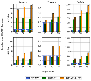
Figure 6: Average speedup per ALS iteration of our distributed randomized algorithms over SPLATT (5 trials).

Figure 6 shows the speedup of our randomized distributed algorithm per ALS round over SPLATT at 4 nodes and 16 nodes. We used the same configuration and sample count for each tensor as Table V-A. On Amazon and Reddit at rank 25 and 4 nodes, d-STS-CP achieves a speedup in the range 5.7x-6.8x while d-CP-ARLS-LEV achieves between 8.0-9.5x. We achieve our most dramatic speedup at rank 75 on the Reddit tensor, with d-STS-CP achieving 10.7x speedup and d-CP-ARLS-LEV achieving 14.6x. Our algorithms achieve less speedup compared to SPLATT on the denser Patents tensor. Here, a larger number nonzeros are selected by randomized sampling, with a significant computation bottleneck in the step that extracts and reindexes the nonzeros from the tensor. The bottom half of Figure 6 shows that d-STS-CP maintains at least a 2x speedup over SPLATT even at 16 nodes / 2048 CPU cores on Amazon and Reddit, but exhibits worse speedup on the Patents tensor. Table V-A quantifies the accuracy sacrificed for the speedup, which can be changed by adjusting the sample count at each least-squares solve. As Figure 1 shows, both of our randomized algorithms make faster progress than SPLATT, with d-STS-CP producing a comparable rank-100 decomposition of the Reddit tensor in under two minutes.

V-C Comparison of Communication Schedules

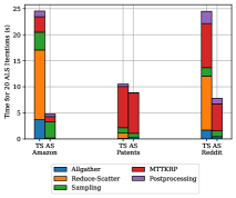
Figure 7: Average runtime (5 trials, $R=25$) per activity for tensor-stationary and accumulator-stationary distributions with 32 MPI ranks over 4 nodes.

Figure 7 breaks down the runtime per phase of the d-STS-CP algorithm for the tensor-stationary and accumulator-stationary schedules on 4 nodes. To illustrate the effect of sampling on the row gathering step, we gather all rows (not just those sampled) for the tensor-stationary distribution, a communication pattern identical to SPLATT. Observe that the Allgather collective under the accumulator-stationary schedule is significantly cheaper for Amazon and Reddit, since only sampled rows are communicated. As predicted, the Reduce-scatter collective accounts for a significant fraction of the runtime for the tensor-stationary distribution on Amazon and Reddit, which have tensor dimensions in the millions. On both tensors, the runtime of this collective is greater than the time required by all other phases combined in the accumulator-stationary schedule. By contrast, both schedules perform comparably on Patents. Here, the Reduce-scatter cost is marginal due to the smaller dimensions of the tensor.

We conclude that sparse tensors with large dimensions can benefit from the accumulator-stationary distribution to reduce communication costs, while the tensor-stationary distribution is optimal for tensors with higher density and smaller dimensions. The difference in MTTKRP runtime between the two schedules is further explored in Section V-F.

V-D Strong Scaling and Runtime Breakdown

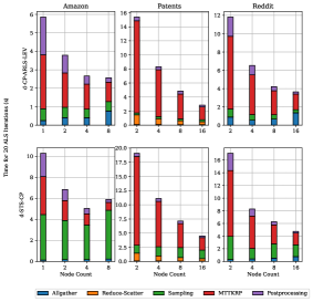
Figure 8: Average runtime (5 trials) per activity vs. node count, $R=25$. Each node has 128 CPU cores, and 8 MPI ranks were used per node. Because times for each segment were averaged across processors, the sum of segment heights in each bar differs slightly from the average total runtime.

Figure 8 gives the runtime breakdown for our algorithms at varying node counts. Besides the All-gather and Reduce-scatter collectives used to communicate rows of the factor matrices, we benchmark time spent in each of the three phases identified in Section IV: sample identification, execution of the downsampled MTTKRP, and post-processing factor matrices.

With its higher density, the Patents tensor has a significantly larger fraction of nonzeros randomly sampled at each linear least-squares solve. As a result, most ALS runtime is spent on the downsampled MTTKRP. The Reddit and Amazon tensors, by contrast, spend a larger runtime portion on sampling and post-processing the factor matrices due to their larger mode sizes. Scaling beyond 4 nodes for the Amazon tensor is impeded by the relatively high sampling cost in d-STS-CP, a consequence of repeated All-to-allv collective calls.

V-E Weak Scaling with Target Rank

We measure weak scaling for our randomized algorithms by recording the throughput (nonzero entries processed in the MTTKRP per second of total algorithm runtime) as both the processor count and target rank $R$ increase proportionally. We keep the ratio of node count to rank $R$ constant at 16. We use a fixed sample count $J=2^{16}$, and we benchmark the d-STS-CP algorithm to ensure minimal accuracy loss as the rank increases.

Although the FLOP count of the MTTKRP is linearly proportional to $R$ (see Equation (6)), we expect the efficiency of the MTTKRP to improve with increased rank due to spatial cache access locality in the longer factor matrix rows, a well-documented phenomenon [36]. On the other hand, the sampling runtime of the d-STS-CP algorithm grows quadratically with the rank $R$ (see Table II). The net impact of these competing effects is determined by the density and dimensions of the sparse tensor.

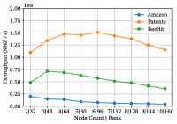
Figure 9: Average throughput (3 trials per data point) of the d-STS-CP algorithm vs. increasing node count and rank, measured as the average number of nonzeros iterated over in the MTTKRP per second of total algorithm runtime (higher is better). Ideal scaling is a horizontal line. The ratio of node count to rank was kept constant at 16. d-STS-CP was chosen to preserve decomposition accuracy at high ranks.

Figure 9 shows the results of our weak scaling experiments. Because ALS on the Amazon tensor spends a large fraction of time drawing samples (see Figure 8), its throughput suffers with increasing rank due to the quadratic cost of sampling. At the other extreme, our algorithm spends little time sampling from the Patents tensor with its smaller dimensions, enabling throughput to increase due to higher cache spatial locality in the factor matrices. The experiments on Reddit follow a middle path between these extremes, with performance dropping slightly at high rank due to the cost of sampling.

V-F Load Imbalance

Besides differences in the communication times of the tensor-stationary and accumulator-stationary schedules, Figure 7 indicates a runtime difference in the downsampled MTTKRP between the two schedules. Figure 10 offers an explanation by comparing the load balance of these methods. We measure load imbalance (averaged over 5 trials) as the maximum number of nonzeros processed in the MTTKRP by any MPI process over the mean of the same quantity.

The accumulator-stationary schedule yields better load balance over all tensors, with a dramatic difference for the case of Amazon. The latter exhibits a few rows of the Khatri-Rao design matrix with high statistical leverage and corresponding fibers with high nonzero counts, producing the imbalance. The accumulator-stationary distribution (aided by the load balancing random permutation) distributes the nonzeros in each selected fiber across all $P$ processors, correcting the imbalance.

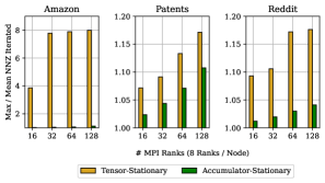
Figure 10: Load imbalance, defined as maximum / mean nonzeros iterated over by any MPI process, for d-STS-CP for varying node count under the tensor-stationary vs. accumulator-stationary communication schedules. 8 MPI ranks were used per node. Each bar is an average of 5 trials.

VI Conclusions and Further Work

We have demonstrated in this work that randomized CP decomposition algorithms are competitive at the scale of thousands of CPU cores with state-of-the-art, highly-optimized non-randomized libraries for the same task. Future work includes improving the irregular communication pattern of the d-STS-CP algorithm, as well as deploying our algorithm on massive real-world tensors larger than those offered by FROSTT.

References

- [1] H.-H. Mao, C.-J. Wu, E. E. Papalexakis, C. Faloutsos, K.-C. Lee, and T.-C. Kao, “MalSpot: Multi2 Malicious Network Behavior Patterns Analysis,” in Advances in Knowledge Discovery and Data Mining, ser. Lecture Notes in Computer Science, V. S. Tseng, T. B. Ho, Z.-H. Zhou, A. L. P. Chen, and H.-Y. Kao, Eds. Cham: Springer International Publishing, 2014, pp. 1–14.
- [2] S. Smith, J. W. Choi, J. Li, R. Vuduc, J. Park, X. Liu, and G. Karypis, “FROSTT: The Formidable Repository of Open Sparse Tensors and Tools,” 2017. [Online]. Available: http://frostt.io/
- [3] I. Balazevic, C. Allen, and T. Hospedales, “TuckER: Tensor Factorization for Knowledge Graph Completion,” in Proceedings of the 2019 Conference on Empirical Methods in Natural Language Processing and the 9th International Joint Conference on Natural Language Processing (EMNLP-IJCNLP). Hong Kong, China: Association for Computational Linguistics, Nov. 2019, pp. 5185–5194.
- [4] B. W. Larsen and T. G. Kolda, “Practical leverage-based sampling for low-rank tensor decomposition,” SIAM J. Matrix Analysis and Applications, June 2022, accepted for publication.
- [5] S. Smith, K. Huang, N. D. Sidiropoulos, and G. Karypis, Streaming Tensor Factorization for Infinite Data Sources, pp. 81–89.
- [6] T. G. Kolda and B. W. Bader, “Tensor Decompositions and Applications,” SIAM Review, vol. 51, no. 3, pp. 455–500, Aug. 2009, publisher: Society for Industrial and Applied Mathematics.
- [7] J. H. Choi and S. Vishwanathan, “DFacTo: Distributed Factorization of Tensors,” in Advances in Neural Information Processing Systems, Z. Ghahramani, M. Welling, C. Cortes, N. Lawrence, and K. Q. Weinberger, Eds., vol. 27. Curran Associates, Inc., 2014.
- [8] S. Smith, N. Ravindran, N. D. Sidiropoulos, and G. Karypis, “SPLATT: Efficient and Parallel Sparse Tensor-Matrix Multiplication,” in 2015 IEEE International Parallel and Distributed Processing Symposium, May 2015, pp. 61–70, iSSN: 1530-2075.
- [9] O. Kaya and B. Uçar, “Scalable sparse tensor decompositions in distributed memory systems,” in SC ’15: Proceedings of the International Conference for High Performance Computing, Networking, Storage and Analysis, 2015, pp. 1–11.
- [10] N. Park, B. Jeon, J. Lee, and U. Kang, “Bigtensor: Mining billion-scale tensor made easy,” in Proceedings of the 25th ACM International on Conference on Information and Knowledge Management, ser. CIKM ’16. New York, NY, USA: Association for Computing Machinery, 2016, p. 2457–2460.
- [11] D. Cheng, R. Peng, Y. Liu, and I. Perros, “SPALS: Fast Alternating Least Squares via Implicit Leverage Scores Sampling,” in Advances in Neural Information Processing Systems, D. Lee, M. Sugiyama, U. Luxburg, I. Guyon, and R. Garnett, Eds., vol. 29. Curran Associates, Inc., 2016.
- [12] O. A. Malik, “More Efficient Sampling for Tensor Decomposition With Worst-Case Guarantees,” in Proceedings of the 39th International Conference on Machine Learning. PMLR, Jun. 2022, pp. 14 887–14 917, iSSN: 2640-3498.
- [13] V. Bharadwaj, O. A. Malik, R. Murray, L. Grigori, A. Buluc, and J. Demmel, “Fast Exact Leverage Score Sampling from Khatri-Rao Products with Applications to Tensor Decomposition,” in Thirty-seventh Conference on Neural Information Processing Systems, 2023. [Online]. Available: https://arxiv.org/pdf/2301.12584.pdf
- [14] M. W. Mahoney, “Randomized algorithms for matrices and data,” Foundations and Trends® in Machine Learning, vol. 3, no. 2, pp. 123–224, 2011.
- [15] P. Drineas and M. W. Mahoney, “RandNLA: Randomized numerical linear algebra,” Commun. ACM, vol. 59, no. 6, p. 80–90, may 2016.
- [16] P.-G. Martinsson and J. A. Tropp, “Randomized numerical linear algebra: Foundations and algorithms,” Acta Numerica, vol. 29, p. 403–572, 2020.
- [17] S. Smith and G. Karypis, “Tensor-matrix products with a compressed sparse tensor,” in Proceedings of the 5th Workshop on Irregular Applications: Architectures and Algorithms, ser. IA¡sup¿3¡/sup¿ ’15. New York, NY, USA: Association for Computing Machinery, 2015.
- [18] I. Nisa, J. Li, A. Sukumaran-Rajam, P. S. Rawat, S. Krishnamoorthy, and P. Sadayappan, “An efficient mixed-mode representation of sparse tensors,” in Proceedings of the International Conference for High Performance Computing, Networking, Storage and Analysis, ser. SC ’19. New York, NY, USA: Association for Computing Machinery, 2019.
- [19] J. Li, Y. Ma, and R. Vuduc, “ParTI! : A parallel tensor infrastructure for multicore cpus and gpus,” Oct 2018, last updated: Jan 2020. [Online]. Available: http://parti-project.org
- [20] A. Nguyen, A. E. Helal, F. Checconi, J. Laukemann, J. J. Tithi, Y. Soh, T. Ranadive, F. Petrini, and J. W. Choi, “Efficient, out-of-memory sparse mttkrp on massively parallel architectures,” in Proceedings of the 36th ACM International Conference on Supercomputing, ser. ICS ’22. New York, NY, USA: Association for Computing Machinery, 2022.
- [21] S. Wijeratne, R. Kannan, and V. Prasanna, “Dynasor: A dynamic memory layout for accelerating sparse mttkrp for tensor decomposition on multi-core cpu,” 2023.
- [22] R. Kanakagiri and E. Solomonik, “Minimum cost loop nests for contraction of a sparse tensor with a tensor network,” 2023.
- [23] S. Smith and G. Karypis, “A Medium-Grained Algorithm for Sparse Tensor Factorization,” in 2016 IEEE International Parallel and Distributed Processing Symposium (IPDPS), May 2016, pp. 902–911, iSSN: 1530-2075.
- [24] G. Ballard, K. Hayashi, and K. Ramakrishnan, “Parallel nonnegative CP decomposition of dense tensors,” in 2018 IEEE 25th International Conference on High Performance Computing (HiPC). IEEE, 2018, pp. 22–31.
- [25] U. Kang, E. Papalexakis, A. Harpale, and C. Faloutsos, “GigaTensor: scaling tensor analysis up by 100 times - algorithms and discoveries,” in Proceedings of the 18th ACM SIGKDD international conference on Knowledge discovery and data mining, ser. KDD ’12. New York, NY, USA: Association for Computing Machinery, Aug. 2012, pp. 316–324.
- [26] L. Ma and E. Solomonik, “Efficient parallel CP decomposition with pairwise perturbation and multi-sweep dimension tree,” in 2021 IEEE International Parallel and Distributed Processing Symposium (IPDPS), May 2021, pp. 412–421, iSSN: 1530-2075.
- [27] E. Solomonik, D. Matthews, J. R. Hammond, J. F. Stanton, and J. Demmel, “A massively parallel tensor contraction framework for coupled-cluster computations,” Journal of Parallel and Distributed Computing, vol. 74, no. 12, pp. 3176–3190, 2014, publisher: Academic Press.
- [28] R. Yadav, A. Aiken, and F. Kjolstad, “Spdistal: Compiling distributed sparse tensor computations,” in Proceedings of the International Conference on High Performance Computing, Networking, Storage and Analysis, ser. SC ’22. IEEE Press, 2022.
- [29] R. Jin, T. G. Kolda, and R. Ward, “Faster Johnson–Lindenstrauss transforms via Kronecker products,” Information and Inference: A Journal of the IMA, vol. 10, no. 4, pp. 1533–1562, 10 2020.
- [30] T. D. Ahle, M. Kapralov, J. B. T. Knudsen, R. Pagh, A. Velingker, D. P. Woodruff, and A. Zandieh, Oblivious Sketching of High-Degree Polynomial Kernels, pp. 141–160.
- [31] H. Diao, Z. Song, W. Sun, and D. Woodruff, “Sketching for kronecker product regression and p-splines,” in International Conference on Artificial Intelligence and Statistics. PMLR, 2018, pp. 1299–1308.
- [32] T. G. Kolda and D. Hong, “Stochastic Gradients for Large-Scale Tensor Decomposition,” SIAM Journal on Mathematics of Data Science, vol. 2, no. 4, pp. 1066–1095, Jan. 2020.
- [33] H.-F. Yu, C.-J. Hsieh, S. Si, and I. Dhillon, “Scalable Coordinate Descent Approaches to Parallel Matrix Factorization for Recommender Systems,” in 2012 IEEE 12th International Conference on Data Mining, Dec. 2012, pp. 765–774, iSSN: 2374-8486.
- [34] E. Chan, M. Heimlich, A. Purkayastha, and R. van de Geijn, “Collective communication: theory, practice, and experience: Research Articles,” Concurrency and Computation: Practice & Experience, vol. 19, no. 13, pp. 1749–1783, Sep. 2007.
- [35] T. B. Rolinger, T. A. Simon, and C. D. Krieger, “Performance considerations for scalable parallel tensor decomposition,” Journal of Parallel and Distributed Computing, vol. 129, pp. 83–98, 2019.
- [36] H. M. Aktulga, A. Buluç, S. Williams, and C. Yang, “Optimizing sparse matrix-multiple vectors multiplication for nuclear configuration interaction calculations,” in 2014 IEEE 28th International Parallel and Distributed Processing Symposium, 2014, pp. 1213–1222.