Uncertainty Quantification in Synthetic Controls
with Staggered Treatment Adoption

Abstract

We propose principled prediction intervals to quantify the uncertainty of a large class of synthetic control predictions (or estimators) in settings with staggered treatment adoption, offering precise non-asymptotic coverage probability guarantees. From a methodological perspective, we provide a detailed discussion of different causal quantities to be predicted, which we call causal predictands, allowing for multiple treated units with treatment adoption at possibly different points in time. From a theoretical perspective, our uncertainty quantification methods improve on prior literature by (i) covering a large class of causal predictands in staggered adoption settings, (ii) allowing for synthetic control methods with possibly nonlinear constraints, (iii) proposing scalable robust conic optimization methods and principled data-driven tuning parameter selection, and (iv) offering valid uniform inference across post-treatment periods. We illustrate our methodology with an empirical application studying the effects of economic liberalization in the 1990s on GDP for emerging European countries. Companion general-purpose software packages are provided in Python, R and Stata.

Keywords: causal inference, synthetic controls, staggered treatment adoption, prediction intervals, non-asymptotic inference.

1 Introduction

The synthetic control method was introduced by Abadie and Gardeazabal (2003), and since then many extensions and generalizations have been proposed in the literature (see Abadie, 2021, and references therein). This methodology is now part of the standard toolkit for program evaluation and treatment effect analysis, offering a complement to traditional difference-in-differences, event studies, and other panel data approaches for causal inference employing longitudinal aggregated data with few treated units. Most of the synthetic control literature concentrates on identification, as well as on prediction or point estimation of treatment effects, under different causal inference frameworks and algorithmic implementations. In contrast, despite its importance for empirical work, principled uncertainty quantification of synthetic control predictions or estimators remains mostly unexplored beyond some specific methods for the canonical single-treatment-unit case.

We develop prediction intervals to quantify the uncertainty of a large class of synthetic control predictions (or estimators) in settings with staggered treatment adoption, offering precise non-asymptotic coverage probability guarantees, scalable robust optimization implementations, and principled tuning parameter selection. Employing a causal inference framework where potential outcomes are assumed to be random, we propose inferential procedures with non-asymptotic probability guarantees; such guarantees are valuable because synthetic control applications often have small sample sizes, limiting the applicability of asymptotic approximations. Conceptually, our proposed prediction intervals capture two sources of uncertainty: one coming from the construction of the synthetic control weights with pre-treatment data, and the other generated by the irreducible sampling variability introduced by the post-treatment outcomes. The proposed prediction intervals also take into account potential misspecification error explicitly, and enjoy other robustness properties due to their non-asymptotic construction.

Our first contribution is methodological in nature due to the complexity added by the staggered treatment adoption setup, which allows for (but does not require) the existence of multiple treatment units changing from control to treatment status at possibly different points in time. In Section 3, we introduce a general causal inference framework that is specifically tailored to synthetic control methods and incorporates staggered treatment adoption. Using this framework, we define different causal quantities to be predicted in the context of synthetic controls, which we refer to as causal predictands, and explain how our inferential methods can be used in each case. Furthermore, our proposed causal framework explicitly allows for misspecification error, multiple covariate features, and cross-equation re-weighting when constructing the synthetic control weights with pre-treatment data.

Building on our general causal inference framework, we present two main theoretical contributions in Section 4. First, we give high-level sufficient conditions leading to valid prediction intervals with precise non-asymptotic guarantees, allowing for stationary and non-stationary data and for synthetic control predictions constructed using multiple re-weighted features and nonlinear constraints. We also provide easy-to-verify primitive conditions, which cover all common synthetic control methods in the literature (e.g., Ridge and elastic net regression). Second, we extend our methods to provide not only pointwise but also joint inference validity across post-treatment time periods. This result allows for the construction of joint “prediction bands” to complement the prediction intervals for different predictands at each point in the post-treatment period.

To complement our methodological and theoretical work, Section 5 discusses scalable robust optimization implementations and principled tuning parameter selection based on our theoretical results. First, we show how to recast our proposed general synthetic control methods for prediction and uncertainty quantification as conic optimization programs (Boyd and Vandenberghe, 2004). This approach gives massive speed improvements for implementation. Second, our proposed methods explicitly employ the non-asymptotic characterizations of the coverage errors associated with the proposed prediction intervals to calibrate the underlying tuning parameters for practice. In particular, we discuss in detail relaxation methods for possibly nonlinear constraints based on our theoretical development. Section 5.4 gives a summary of our algorithmic implementation.

We illustrate our methods with an empirical application investigating the effect of economic liberalization in the 1990s on GDP for emerging European countries. This empirical work is motivated by Billmeier and Nannicini (2013) who, also employing synthetic control methods, studied the same substantive question for countries in other regions of the world. Our main findings suggest that economic liberalization in the 1990s did not have a positive economic impact for emerging European countries. This finding is in line with prior empirical results. The Supplemental Appendix provides additional empirical evidence supporting our main findings, including a re-analysis using alternative synthetic control predictions for different countries and a discussion of specific cases where the synthetic control method does not appear to be well-suited for the analysis.

We provide general-purpose software implementing all our results in Python, R, and Stata, including detailed documentation and additional replication materials. This software is presented in detail in our companion article Cattaneo, Feng, Palomba and Titiunik (2023), where we discuss several implementation issues related to numerical optimization and tuning parameter selection. To complement the illustration, in Section S.4 of the Supplemental Appendix, we provide more details on how to prepare the data to analyze staggered treatment adoption using synthetic control methods using our companion software.

1.1 Related Literature

Our paper contributes to two strands of the synthetic control literature. First, it contributes to the development of prediction/estimation and inference methods for staggered treatment adoption settings. Putting aside generic linear factor model or matrix completion methods, Ben-Michael, Feller and Rothstein (2022) and Shaikh and Toulis (2021) appear to be the only prior papers that have studied staggered treatment adoption for synthetic controls. The first paper focuses on prediction/estimation in settings where the pre-treatment fit is poor, and develops penalization methods for improving the performance of the canonical synthetic control method. Ben-Michael, Feller and Rothstein (2022) also suggest employing a bootstrap method for assessing uncertainty, but no formalization is provided guaranteeing its (asymptotic) validity. Shaikh and Toulis (2021) focus on uncertainty quantification employing a parametric duration model and propose a permutation-based inferential method under a symmetry assumption. Our paper complements these prior works by offering a nonparametric inference method with demonstrable non-asymptotic coverage guarantees and allowing for misspecification in the construction of the synthetic control weights, which can be applied directly to a large class of synthetic control (possibly penalized) predictions and causal quantities of interest.

Second, from a general methodological perspective, our proposed inference methods are motivated by Vovk (2012), and are most closely related to prior work by Chernozhukov, Wüthrich and Zhu (2021a, b) on conformal prediction intervals and by Cattaneo, Feng and Titiunik (2021) on non-asymptotic prediction intervals (see Wainwright (2019) for a modern introduction to non-asymptotic statistical learning). We contribute to this second strand of the literature by developing new prediction interval methods. First, we allow for a large class of causal predictands in staggered adoption settings (prior work covered only the canonical single treated unit case). Second, we cover a large class of synthetic control predictions with possibly nonlinear constraints (prior work allowed for predictions with linear constraints). Third, we develop scalable robust optimization implementations and propose principled data-driven tuning parameter selection (prior work did not provide guidance on these issues). Fourth, we develop valid uniform inference across post-treatment periods (absent in prior work).

There are a few other recent proposals in the literature to quantify uncertainty and conduct inference for synthetic controls. For example, Li (2020) study correctly specified linear factor models, Masini and Medeiros (2021) study high-dimensional penalization methods, Agarwal, Shah, Shen and Song (2021) investigate matrix completion methods, Shen, Ding, Sekhon and Yu (2022) explore panel data methods, and Shi, Miao, Hu and Tchetgen (2023) develop inference methods using a proximal causal inference framework. All these methods rely on asymptotic approximations, in most cases employing standard Gaussian critical values that assume away misspecification errors and other small sample issues. Our work complements these contributions by providing prediction intervals with non-asymptotic coverage guarantees. Finally, all the inferential methods mentioned so far contrast with the original method proposed by Abadie, Diamond and Hainmueller (2010), which relies on design-based permutation of treatment assignment assuming that the potential outcomes are non-random.

2 The Effect of Liberalization on GDP for Emerging European Countries

During the second half of the twentieth century, a considerable number of countries all over the world launched programs of (external) economic liberalization, booming from 22% in 1960 to 73% in the early 2000s (Wacziarg and Welch, 2008). In the last thirty years, political scientists and economists have investigated the social and economic consequences of such liberalization programs, often reaching conflicting conclusions (see, e.g., Levine and Renelt, 1992; Sachs, Warner, Åslund and Fischer, 1995; DeJong and Ripoll, 2006).

The impact of liberalization policies on economic welfare has been traditionally investigated with cross-country analyses (e.g. Sachs, Warner, Åslund and Fischer, 1995) and individual case studies (e.g. Bhagwati and Srinivasan, 2001). More recently, scholars have turned to synthetic control methods in the hope of employing a causal inference methodology that allows for the presence of time-varying unobservable confounders. Employing the synthetic control framework originally developed in Abadie and Gardeazabal (2003), Billmeier and Nannicini (2013) analyzed the effects of liberalization in four continents: Africa, Asia, North America, and South America. They used a pre-existing dataset of economic variables (previously used in Giavazzi and Tabellini, 2005) which includes 180 countries, covers the period 1963–2000, and contains an indicator for economic liberalization originally defined in Sachs, Warner, Åslund and Fischer (1995) and updated in Wacziarg and Welch (2008) (hereafter, the Sachs-Warner indicator). More details on the data and the definition of economic liberalization can be found in the Supplemental Appendix Section S.4.

The main finding of Billmeier and Nannicini (2013) is that economic liberalization—as measured by the Sachs-Warner indicator—has a non-negative effect on GDP per capita. Moreover, the authors document the presence of substantial heterogeneity in the effects depending on the period of time in which the liberalization took place. On the one hand, the predicted effect on real income per capita is positive in those countries that embarked on programs of economic liberalization before the 1980s. On the other hand, in the MENA (Middle East and North Africa) region and in sub-Saharian Africa, where many liberalization episodes occurred after 1985, the magnitude of the predicted effect becomes either statistically insignificant or economically irrelevant.

Our work builds on Billmeier and Nannicini (2013) in three ways. First, we form prediction intervals around causal predictions using our new methodology. Second, rather than constructing a synthetic control independently for each treated unit, we leverage both the presence of multiple treated units and the staggered nature of treatment adoption to jointly form the synthetic controls. Third, by borrowing donors from other continents, we also analyze the impact of economic liberalization events in Europe (see Table 1 below).

Table 1: Economic liberalization episodes in the Billmeier and Nannicini (2013) dataset.

Country	Event	Years	Years	Analyzed in
Name	Date	Closed	Liberalized	this work
Albania	1992	29	9	$\checkmark$
Bulgaria	1991	28	10	$\checkmark$
Czech Republic	1991	28	10	$\checkmark$
Hungary	1990	27	11	$\checkmark$
North Macedonia	1994	31	7	✗
Poland	1990	27	11	$\checkmark$
Romania	1992	29	9	$\checkmark$
Slovak Republic	1991	28	10	$\checkmark$
Slovenia	1991	28	10	✗

Notes: a comprehensive description of the events that led the Sachs-Warner indicator to switch on for these countries is contained in the Supplemental Appendix Section S.4 together with the full set of donors.

As shown in Table 1, we study seven liberalization episodes that occurred in Europe out of the nine available ones. In particular, North Macedonia is not included in the final analysis due to the lack of other variables in the dataset besides GDP per capita before 1994, whereas Slovenia is excluded in virtue of the poor pre-treatment fit yielded by the synthetic controls for such country. We discover that the real income per capita trajectory during the 10 years following the liberalization is lower than it would have been in the absence of the liberalization in all countries we analyzed. Similarly, the average post-treatment effect is negative for all the treated units and so is the average post-treatment effect on the treated (see Section 3 for a precise definitions). However, when individual and simultaneous prediction intervals are taken into account, the trajectory of the synthetic control becomes indistinguishable from the realized time series for real income with high probability. Only the average treatment effect on the treated differs from zero with high probability. Results in other continents—fully presented in the Supplemental Appendix Section S.6—confirm in magnitude the ones found in Billmeier and Nannicini (2013), whenever it has been possible to compare them. However, the data do not allow us to draw the conclusion that liberalization events changed the trajectory of GDP per capita in either a favorable or negative way.

3 Causal Inference Framework and Quantities of Interest

We consider the synthetic control (SC) framework with a fixed number of units that may adopt treatment at different times. Specifically, a researcher observes $N$ units for $T$ time periods. Units are indexed by $i=1,\ldots,N$, and time periods are indexed by $t=1,\ldots,T$. Let $T_{i}$ represent the time when unit $i$ receives the treatment, with $T_{i}=\infty$ denoting that unit $i$ is never treated (at least during the observed $T$ time periods). Each unit $i$ remains untreated in $t=1,\ldots,T_{i}-1$ and remains treated since $T_{i}$. We assume that there is a (non-empty) set of units that are never treated, i.e., $N_{0}:=\sum_{i=1}^{N}\mathds{1}(T_{i}=\infty)>0$, and let $N_{1}:=N-N_{0}$ be the number of units that are eventually treated by time period $T$. Without loss of generality, assume units are ordered in the adoption time: $T_{1}\leq T_{2}\leq\cdots\leq T_{N_{1}}$. In our empirical application, the treatment of interest is economic liberalization, the adoption time of which is heterogeneous across different countries.

The staggered adoption problem can be analyzed in a multi-valued treatment effects framework. Let $Y_{it}(s)$ denote the potential outcome of unit $i$ in period $t$ that would be observed if unit $i$ had adopted the treatment in period $s$, for $s=1,\ldots,T,\infty$, and we set $Y_{it}(s)=Y_{it}(\infty)$ for $t<s$. Implicitly, these simplifications impose two standard assumptions: no spillovers (the potential outcomes of unit $i$ depend only on $i$’s adoption time) and no anticipation (a unit’s potential outcomes prior to the treatment are equal to the outcomes it would have had if it had never been treated). Then, the observed outcome can be written as

$$Y_{it}=Y_{it}(\infty)\mathds{1}(t<T_{i})+Y_{it}(T_{i})\mathds{1}(t\geq T_{i}).$$

A large set of causal predictands can be defined in this context. In particular, for $k\geq 0$, let $\tau_{ik}$ be the (individual) treatment effect of unit $i$ in $T_{i}+k$ ($k$ periods after treatment adoption):

$$\tau_{ik}:=Y_{i(T_{i}+k)}(T_{i})-Y_{i(T_{i}+k)}(\infty).$$

This is the treatment effect of interest in the classical synthetic control analysis with only one treated unit. When multiple treated units or multiple post-treatment periods are available, a researcher might be interested in a variety of other causal predictands. The following are some typical examples:

1. Average post-treatment effect on unit $i$:

   $$\tau_{i\cdot}:=\frac{1}{T-T_{i}+1}\sum_{k=0}^{T-T_{i}}\tau_{ik}\;.$$

2. Average treatment effect on units treated at time $s_{0}$, $k$ periods after treatment adoption:

   $$\tau_{\cdot k,s_{0}}:=\frac{1}{|\{i:T_{i}=s_{0}\}|}\sum_{i:T_{i}=s_{0}}\tau_{ik}\;,$$

   where $|\{i:T_{i}=s_{0}\}|$ denotes the number of units that get treated at $s_{0}$.

3. Average treatment effect on the treated, $k$ periods after treatment adoption:

   $$\tau_{\cdot k}:=\frac{1}{N_{1}}\sum_{i=1}^{N_{1}}\tau_{ik}\;.$$

Since the observation ends at time $T$, the number of treated units included in the definition of the average treatment effect $\tau_{\cdot k}$ could vary across $k$. To avoid this complication, we assume that all treated units are observed at least $K$ periods after the treatment for some $K\geq 1$, i.e., $T_{N_{1}}\leq T-K$, and attention is restricted to $\tau_{\cdot k}$ for $k\leq K$ only.

The potential outcomes, treatment adoption times, and individual treatment effects are viewed as random quantities in general. We assume that there is only a fixed (possibly small) number of treated units and time periods, which is often the case in synthetic control applications. Thus, the various average treatment effects defined above are also random quantities in general, but we continue to refer to them as “treatment effects” to be consistent with analogous quantities defined in the literature (e.g., assuming a fixed, non-random potential outcomes framework). In classical large-sample-based causal analysis, target parameters are often probability or ergodic (non-random) limits of the average effects above as $N_{1}\rightarrow\infty$, $T-T_{i}\rightarrow\infty$, and/or $K\rightarrow\infty$; our results are also valid in such settings. Nevertheless, in this paper we develop statistical inference methods based on prediction intervals that describe a region where a new realization of a (random) causal predictand of interest is likely to be observed, rather than usual confidence intervals giving a region in the parameter space for a non-random parameter of interest.

The canonical synthetic control analysis with one single treated unit can be viewed as a special case of the more general setup described above. Specifically, suppose that unit $1$ is the only treated unit who receives the treatment at $T_{1}$, and all other units are never treated, i.e., $T_{i}=\infty$ for all $i\geq 2$. Then, the observed outcome is

$$Y_{it}=\begin{cases}Y_{it}(\infty)\quad&i=2,\ldots,N\\ Y_{1t}(\infty)\quad&i=1\text{ and }t=1,\ldots,T_{1}-1\\ Y_{1t}(T_{1})\quad&i=1\text{ and }t=T_{1},\ldots,T\\ \end{cases}.$$

The target causal predictand in this canonical case is usually the individual treatment effect on the treated, i.e., $\tau_{1k}$ defined previously.

3.1 Synthetic Control Method

Consider the case where multiple treated units are available, and one would like to find a vector of SC weights possibly different for each treated unit. From now on, we use a superscript $i=1,\ldots,N_{1}$ in brackets to index the treated units that enter the construction of the desired causal predictand, and a subscript $l=1,\ldots,M$ to denote different features of the treated on which one would like to match.

Let $\mathbf{A}_{l}^{[i]}=(a_{1,l}^{[i]},\cdots,a_{T_{0},l}^{[i]})^{\prime}\in\mathbb{R}^{T_{0}}$ be the $l$th feature of the treated unit $i$ measured in $T_{0}$ (user-specified) pre-treatment periods. For each feature $l$ and each treated unit $i$, there exist $J+K$ variables that are used to predict or match the $T_{0}$-dimensional vector $\mathbf{A}_{l}^{[i]}$. These $J+K$ variables are separated into two groups denoted by $\mathbf{B}_{l}^{[i]}=(\mathbf{B}_{1,l}^{[i]},\mathbf{B}_{2,l}^{[i]},\cdots,\mathbf{B}_{J,l}^{[i]})\in\mathbb{R}^{T_{0}\times J}$ and $\mathbf{C}_{l}^{[i]}=(\mathbf{C}_{1,l}^{[i]},\cdots,\mathbf{C}_{K,l}^{[i]})\in\mathbb{R}^{T_{0}\times K}$, respectively. More precisely, for each $j=1,\ldots,J$, $\mathbf{B}_{j,l}^{[i]}=(b_{j1,l}^{[i]},\cdots,b_{jT_{0},l}^{[i]})^{\prime}$ corresponds to the $l$th feature of the $j$th unit in the donor pool measured in $T_{0}$ pre-treatment periods, and for each $k=1,\ldots,K$, $\mathbf{C}_{k,l}^{[i]}=(c_{k1,l}^{[i]},\cdots,c_{kT_{0},l}^{[i]})^{\prime}$ is another vector of control variables used to predict $\mathbf{A}_{l}^{[i]}$ over the same pre-intervention time span. Stacking the $M$ equations (corresponding to $M$ features) for each treated unit, we define

$$\underbrace{\mathbf{A}^{[i]}}_{T_{0}\cdot M\times 1}=\begin{bmatrix}\mathbf{A}_{1}^{[i]}\\ \vdots\\ \mathbf{A}_{M}^{[i]}\end{bmatrix},\quad\underbrace{\mathbf{B}^{[i]}}_{T_{0}\cdot M\times J}=\begin{bmatrix}\mathbf{B}_{1}^{[i]}\\ \vdots\\ \mathbf{B}_{M}^{[i]}\end{bmatrix},\quad\underbrace{\mathbf{C}^{[i]}}_{T_{0}\cdot M\times K\cdot M}=\begin{bmatrix}\mathbf{C}_{1}^{[i]}&\mathbf{0}&\cdots&\mathbf{0}\\ \mathbf{0}&\mathbf{C}_{2}^{[i]}&\cdots&\mathbf{0}\\ \vdots&\vdots&\ddots&\vdots\\ \mathbf{0}&\mathbf{0}&\cdots&\mathbf{C}_{M}^{[i]}\end{bmatrix}.$$

In our empirical application, $\mathbf{A}^{[i]}$ contains the (log) GDP per capita and the percentage of complete secondary schooling in population ($M=2$) of a treated economy $i$ (that has ever experienced liberalization) during the pre-liberalization period, and $\mathbf{B}^{[i]}$ contains the same two features of the donor economies used to match $\mathbf{A}^{[i]}$. For each feature $l=1,2$, $\mathbf{C}_{l}^{[i]}$ contains an intercept and a linear time trend ($K=2$).

The goal of the synthetic control method is to search for a vector of weights $\mathbf{w}=(\mathbf{w}^{[1]\prime},\cdots,\mathbf{w}^{[N_{1}]\prime})^{\prime}\in\mathcal{W}\subseteq\mathbb{R}^{JN_{1}}$ which is common across the $M$ features and a vector of coefficients $\mathbf{r}=(\mathbf{r}^{[1]\prime},\cdots,\mathbf{r}^{[N_{1}]\prime})^{\prime}\in\mathcal{R}\subseteq\mathbb{R}^{KMN_{1}}$, such that the linear combination of $\mathbf{B}^{[i]}$ and $\mathbf{C}^{[i]}$ matches $\mathbf{A}^{[i]}$ as closely as possible, for all $1\leq i\leq N_{1}$. The feasibility sets $\mathcal{W}$ and $\mathcal{R}$ capture the restrictions imposed. Typical examples include simplex-type, lasso-type and ridge-type constraints (for further details, see Cattaneo, Feng, Palomba and Titiunik, 2023).

Such SC weights are typically obtained via the following optimization problem: for some $(T_{0}\cdot M\cdot N_{1})\times(T_{0}\cdot M\cdot N_{1})$ symmetric weighting matrix $\mathbf{V}$,

$$\widehat{\bm{\beta}}:=(\widehat{\mathbf{w}}^{\prime},\;\widehat{\mathbf{r}}^{\prime})^{\prime}\in\underset{\mathbf{w}\in\mathcal{W},\,\mathbf{r}\in\mathcal{R}}{\operatorname*{arg\,min}}\;(\mathbf{A}-\mathbf{B}\mathbf{w}-\mathbf{C}\mathbf{r})^{\prime}\mathbf{V}(\mathbf{A}-\mathbf{B}\mathbf{w}-\mathbf{C}\mathbf{r})$$ (3.1)

where

$$\underbrace{\mathbf{A}}_{T_{0}\cdot M\cdot N_{1}\times 1}=\begin{bmatrix}\mathbf{A}^{[1]}\\ \vdots\\ \mathbf{A}^{[N_{1}]}\end{bmatrix},\;\underbrace{\mathbf{B}}_{T_{0}\cdot M\cdot N_{1}\times J\cdot N_{1}}=\begin{bmatrix}\mathbf{B}^{[1]}&\mathbf{0}&\cdots&\mathbf{0}\\ \mathbf{0}&\mathbf{B}^{[2]}&\cdots&\mathbf{0}\\ \vdots&\vdots&\ddots&\vdots\\ \mathbf{0}&\mathbf{0}&\cdots&\mathbf{B}^{[N_{1}]}\end{bmatrix},\;\underbrace{\mathbf{C}}_{T_{0}\cdot M\cdot N_{1}\times K\cdot M\cdot N_{1}}=\begin{bmatrix}\mathbf{C}^{[1]}&\mathbf{0}&\cdots&\mathbf{0}\\ \mathbf{0}&\mathbf{C}^{[2]}&\cdots&\mathbf{0}\\ \vdots&\vdots&\ddots&\vdots\\ \mathbf{0}&\mathbf{0}&\cdots&\mathbf{C}^{[N_{1}]}\end{bmatrix}.$$

Accordingly, we write $\widehat{\mathbf{w}}=(\widehat{\mathbf{w}}^{[1]\prime},\cdots,\widehat{\mathbf{w}}^{[N_{1}]\prime})^{\prime}$ where each $\widehat{\mathbf{w}}^{[i]}=(\widehat{w}_{1}^{[i]},\cdots,\widehat{w}_{J}^{[i]})^{\prime}$ is the SC weights on $J$ control units that are used to predict the counterfactual of the treated unit $i$. Similarly, write $\widehat{\mathbf{r}}=(\widehat{\mathbf{r}}^{[1]\prime},\cdots,\widehat{\mathbf{r}}^{[N_{1}]\prime})^{\prime}$ and $\widehat{\bm{\beta}}=(\widehat{\bm{\beta}}^{[1]\prime},\cdots,\widehat{\bm{\beta}}^{[N_{1}]\prime})^{\prime}$.

Then, the predicted counterfactual outcome of each treated unit is given by

$$\widehat{Y}_{it}(\infty):=\mathbf{x}_{t}^{[i]\prime}\widehat{\mathbf{w}}^{[i]}+\mathbf{g}_{t}^{[i]\prime}\widehat{\mathbf{r}}^{[i]}=\mathbf{p}_{t}^{[i]\prime}\widehat{\bm{\beta}}^{[i]},\quad\mathbf{p}_{t}^{[i]}=(\mathbf{x}_{t}^{[i]\prime},\;\mathbf{g}_{t}^{[i]\prime})^{\prime},\quad i=1,\cdots,N_{1},\quad t>T_{i},$$

where $\mathbf{x}_{t}^{[i]}$ is a vector of predictors of the control units measured in time $t$ used to predict the counterfactual of the treated unit $i$, and $\mathbf{g}_{t}^{[i]}$ is a vector of predictors that correspond to the additional control variables specified in $\mathbf{C}^{[i]}$. In our empirical application, $\mathbf{x}_{t}^{[i]}$ is the post-treatment (log) GDP per capita of donor economies, and $\mathbf{g}_{t}^{[i]}$ includes a constant, a linear time trend and two zeros so that $\mathbf{g}_{t}^{[i]}$ is conformable with $\widehat{\mathbf{r}}^{[i]}$. In general, however, variables included in $\mathbf{x}_{t}^{[i]}$ and $\mathbf{g}_{t}^{[i]}$ need not be the same as those in $\mathbf{B}^{[i]}$ and $\mathbf{C}^{[i]}$. For convenience of later exposition, we write $\mathbf{p}_{t}=(\mathbf{p}_{t}^{[1]\prime},\cdots,\mathbf{p}_{t}^{[N_{1}]\prime})^{\prime}$.

Any causal predictand $\tau$ discussed before can be written as the difference between an observed outcome (possibly a linear combination of outcomes of a few treated units or in different periods) and the corresponding counterfactual outcome. To construct a prediction $\widehat{\tau}$ of $\tau$, one only needs to substitute a “SC prediction” for the unobserved counterfactual:

$$\textsf{SC prediction}:=\mathbf{p}_{\tau}^{\prime}\widehat{\bm{\beta}},$$

where the predictor vector $\mathbf{p}_{\tau}$ needs to be defined in context. More details are provided in the following examples.

Example 3.1 (Individual Treatment Effect, $\tau_{ik}$).

Suppose that the individual treatment effect $\tau_{ik}$ of the treated unit $i$ with $T_{i}<\infty$ is of interest for some $0\leq k\leq T-T_{i}$. Let the set of pre-treatment periods be $\{t:t\leq T_{i}-1\}$. The donor pool consists of units that receive treatment later than $T_{i}+k$, i.e., $\{j:T_{j}>T_{i}+k\}$. The SC weights are constructed using the data of the treated unit $i$ and the control units in the pre-treatment period. Given the prediction of the counterfactual outcome $\widehat{Y}_{i(T_{i}+k)}$, the predicted treatment effect is

$$\widehat{\tau}_{ik}:=Y_{i(T_{i}+k)}-\widehat{Y}_{i(T_{i}+k)}(\infty)=Y_{i(T_{i}+k)}-\mathbf{p}_{\tau_{ik}}^{\prime}\widehat{\bm{\beta}}.$$

The predictor vector $\mathbf{p}_{\tau_{ik}}$ in this case is given by

$$\mathbf{p}_{\tau_{ik}}:=(\underbrace{\mathbf{0}_{J+KM}^{\prime},\cdots,\mathbf{0}_{J+KM}^{\prime}}_{(i-1)\text{ vectors}},\;\mathbf{p}_{T_{i}+k}^{[i]\prime},\;\underbrace{\mathbf{0}_{J+KM}^{\prime},\cdots,\mathbf{0}_{J+KM}^{\prime}}_{(N_{1}-i)\text{ vectors}})^{\prime}.$$

where $\mathbf{0}_{J+KM}$ is a $(J+KM)$-vector of zeros. See Figure 1 for a graphical representation of $\widehat{\tau}_{ik}$.

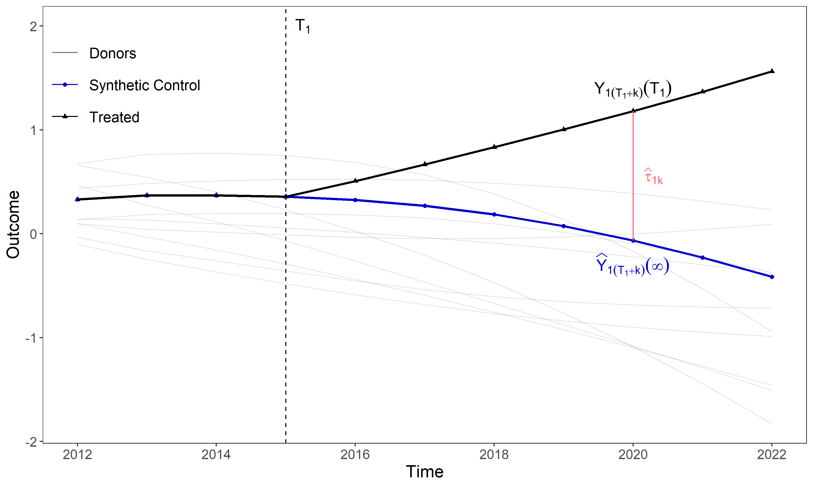
Figure 1: Graphical illustration of the individual treatment effect, $\widehat{\tau}_{ik}$.

Notes: The black line displays the times series of the treated unit’s outcome, whereas the blurred gray lines portray the same variable for the donor units. The blue line is the synthetic control constructed out of the donor units using a simplex-type constraint. The pink vertical line represents the quantity $\widehat{\tau}_{ik}$ described in Example 3.1, where $k$ is set to 5.

Example 3.2 (Average Post-Treatment Effect, $\tau_{i\cdot}$).

Suppose that the quantity of interest is the treatment effect on the treated unit $i$ averaged across all the post-treatment periods, i.e., $\tau_{i\cdot}$ defined previously. Let the set of pre-treatment periods be $\{t:t\leq T_{i}-1\}$, and take the set of all units that are never treated as the donor pool, i.e., $\{j:T_{j}=\infty\}$. The SC weights in this scenario can be constructed in the same way as in the case of individual treatment effects. The prediction of the average post-treatment effect is given by

$$\widehat{\tau}_{i\cdot}:=\frac{1}{T-T_{i}+1}\sum_{t=T_{i}}^{T}\Big{(}Y_{it}-\widehat{Y}_{it}(\infty)\Big{)}=\frac{1}{T-T_{i}+1}\sum_{t=T_{i}}^{T}Y_{it}\;-\;\mathbf{p}_{\tau_{i\cdot}}^{\prime}\widehat{\bm{\beta}},$$

where the predictor vector in this case is given by

$$\mathbf{p}_{\tau_{i\cdot}}:=\Big{(}\underbrace{\mathbf{0}_{J+KM}^{\prime},\cdots,\mathbf{0}_{J+KM}^{\prime}}_{(i-1)\text{ vectors}},\;\frac{1}{T-T_{i}+1}\sum_{t\geq T_{i}}\mathbf{p}_{t}^{[i]\prime},\;\underbrace{\mathbf{0}_{J+KM}^{\prime},\cdots,\mathbf{0}_{J+KM}^{\prime}}_{(N_{1}-i)\text{ vectors}}\Big{)}^{\prime}.$$

See Figure 2 for a graphical representation of $\widehat{\tau}_{i\cdot}$.

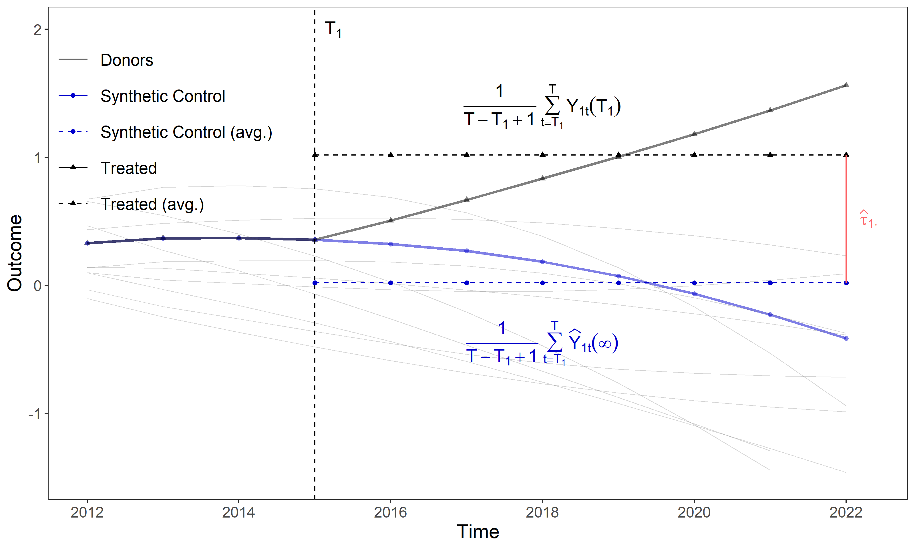
Figure 2: Graphical illustration of the average post-treatment effect, $\widehat{\tau}_{i\cdot}$.

Notes: The black line displays the times series of the treated unit’s outcome, whereas the blurred gray lines portray the same variable for the donor units. The blue line is the synthetic control constructed out of the donor units using a simplex-type constraint. The dashed lines represent the post-treatment average of the treated time series (black) and the synthetic control time series (blue). The pink vertical line represents the quantity $\widehat{\tau}_{i\cdot}$ described in Example 3.2.

Example 3.3 (Average Treatment Effect on the Treated at $s_{0}$ after $k$ Periods, $\tau_{\cdot k,s_{0}}$).

Suppose that the causal predictand of interest is the average treatment effect for units that adopt the treatment at time $s_{0}$, $k$ periods after treatment adoption, i.e., $\tau_{\cdot k,s_{0}}$ defined above. Let the set of pre-treatment periods be $\{t:t\leq s_{0}-1\}$, and take the set of units that adopt the treatment later than $s_{0}+k$, i.e., $\{j:T_{j}>s_{0}+k\}$, as the donor pool. We have two different strategies to conduct the SC analysis:

• Implement the procedure described above, which allows for different SC weights on different treated units. Suppose $\{i:T_{i}=s_{0}\}=\{i_{1},\cdots,i_{n_{s_{0}}}\}$. Then, the predicted effect is given by

  $$\widehat{\tau}_{\cdot k,s_{0}}:=\frac{1}{n_{s_{0}}}\sum_{i:T_{i}=s_{0}}\Big{(}Y_{i(s_{0}+k)}-\widehat{Y}_{i(s_{0}+k)}(\infty)\Big{)}=\frac{1}{n_{s_{0}}}\sum_{i:T_{i}=s_{0}}Y_{i(s_{0}+k)}\;-\;\mathbf{p}_{\tau_{\cdot k,s_{0}}}^{\prime}\widehat{\bm{\beta}},$$

  where the predictor vector in this case is given by

  $$\mathbf{p}_{\tau_{\cdot k,s_{0}}}:=\Big{(}\underbrace{\mathbf{0}_{J+KM}^{\prime},\cdots,\mathbf{0}_{J+KM}^{\prime}}_{(i_{1}-1)\text{ vectors}},\;\;\frac{1}{n_{s_{0}}}\mathbf{p}_{s_{0}+k}^{[i_{1}]\prime},\cdots,\frac{1}{n_{s_{0}}}\mathbf{p}_{s_{0}+k}^{[i_{n_{s_{0}}}]\prime},\;\;\underbrace{\mathbf{0}_{J+KM}^{\prime},\cdots,\mathbf{0}_{J+KM}^{\prime}}_{(N_{1}-i_{n_{s_{0}}})\text{ vectors}}\Big{)}^{\prime}.$$

• Aggregate different treated units into one single unit, denoted by “ave”, whose potential outcomes are given by the average of all units treated at time $s_{0}$:

  $$Y_{t}^{\texttt{ave}}(s;s_{0}):=\frac{1}{n_{s_{0}}}\sum_{i:T_{i}=s_{0}}Y_{it}(s),\quad t=1,\ldots,T,\quad s=1,\ldots,T,\infty.$$

  More precisely, $Y_{t}^{\texttt{ave}}(s;s_{0})$ is the potential outcome of the aggregate unit ave in period $t$ that would be observed if it had adopted the treatment in period $s$, while ave actually adopted the treatment in period $s_{0}$. Other features of this aggregate unit can be constructed similarly as the average of multiple units treated at $s_{0}$. The SC weights can be obtained using the data of the aggregate unit ave and control units in the donor pool from pre-treatment period. Then, the SC analysis proceeds exactly the same way as in Example 3.1. See Figure 3 for a graphical representation of $\widehat{\tau}_{\cdot k,s_{0}}$.

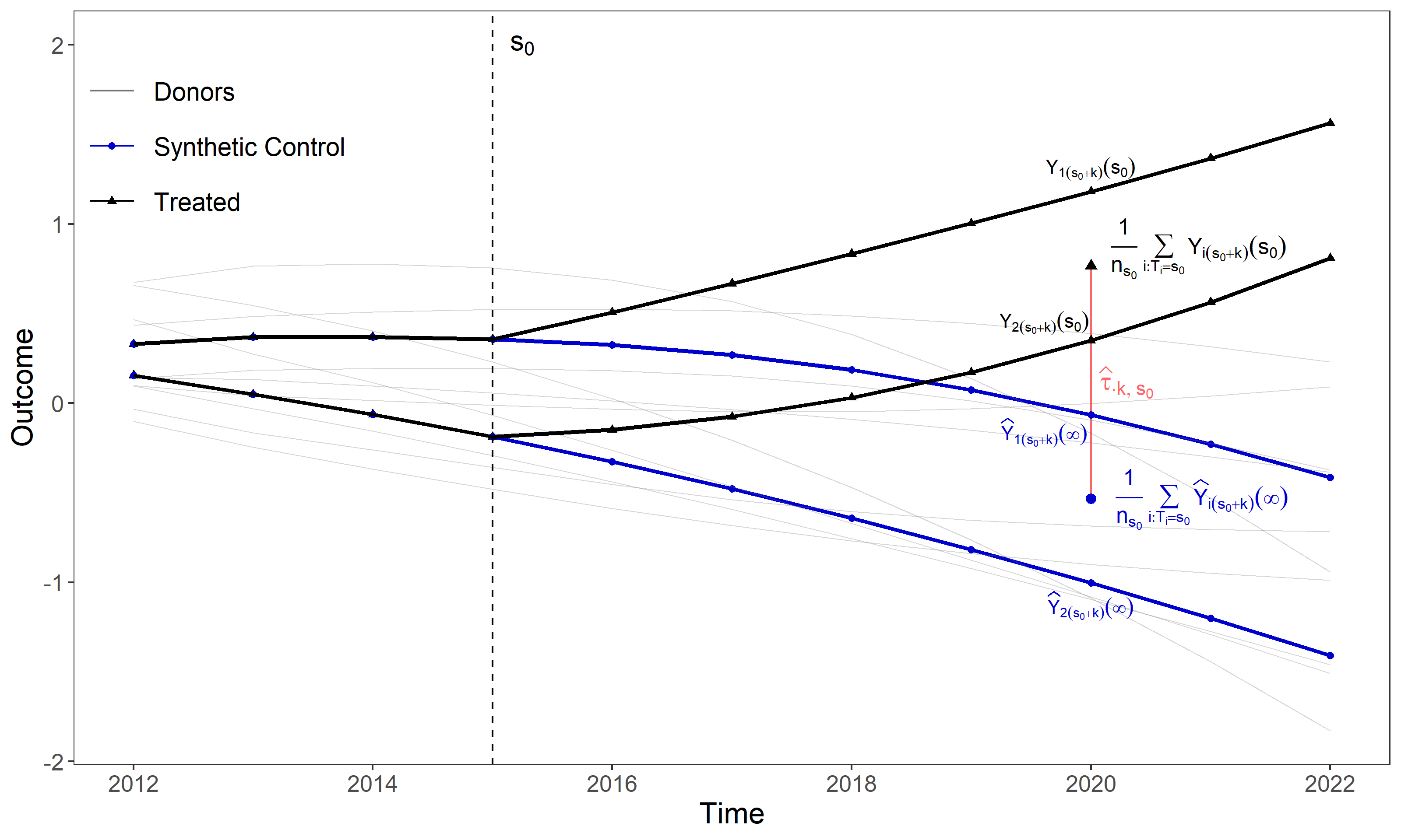
Figure 3: Graphical illustration of the average treatment effect on the treated at $s_{0}$ after $k$ periods, $\widehat{\tau}_{\cdot k,s_{0}}$.

Notes: The black lines display the times series of the treated units’ outcome, whereas the blurred gray lines portray the same variable for the donor units. The blue lines are the synthetic controls constructed out of the donor units using a simplex-type constraint. The largest black triangle represents the average of the treated units’ outcomes at $s_{0}+k$, with $s_{0}$ set to 2015 and $k$ set to 5. Similarly, the largest blue circle is the average of the synthetic controls at $s_{0}+k$. The pink vertical line represents the quantity $\widehat{\tau}_{\cdot k,s_{0}}$ described in Example 3.3. $n_{s_{0}}$ denotes the number of treated units that received the treatment at time $s_{0}$.

Example 3.4 (Average Treatment Effect on all Treated after $k$ Periods, $\tau_{\cdot k}$).

Suppose that the quantity of interest is the average treatment effect for all treated units $k$ periods after treatment adoption, i.e., $\tau_{\cdot k}$ defined above. Let the set of pre-treatment periods be $\{t:t\leq T_{1}-1\}$ and the donor pool be $\{j:T_{j}=\infty\}$. Then, the predicted effect is given by

$$\widehat{\tau}_{\cdot k}:=\frac{1}{N_{1}}\sum_{i=1}^{N_{1}}\Big{(}Y_{i(T_{i}+k)}-\widehat{Y}_{i(T_{i}+k)}\Big{)}=\frac{1}{N_{1}}\sum_{i=1}^{N_{1}}Y_{it}\;-\;\mathbf{p}_{\tau_{\cdot k}}^{\prime}\widehat{\bm{\beta}},$$

where the predictor vector in this case is given by

$$\mathbf{p}_{\tau_{\cdot k}}:=\Big{(}\frac{1}{N_{1}}\mathbf{p}_{T_{1}+k}^{[1]\prime},\cdots,\frac{1}{N_{1}}\mathbf{p}_{T_{N_{1}}+k}^{[N_{1}]\prime}\Big{)}^{\prime}.$$

See Figure 4 for a graphical representation of $\widehat{\tau}_{\cdot k}$.

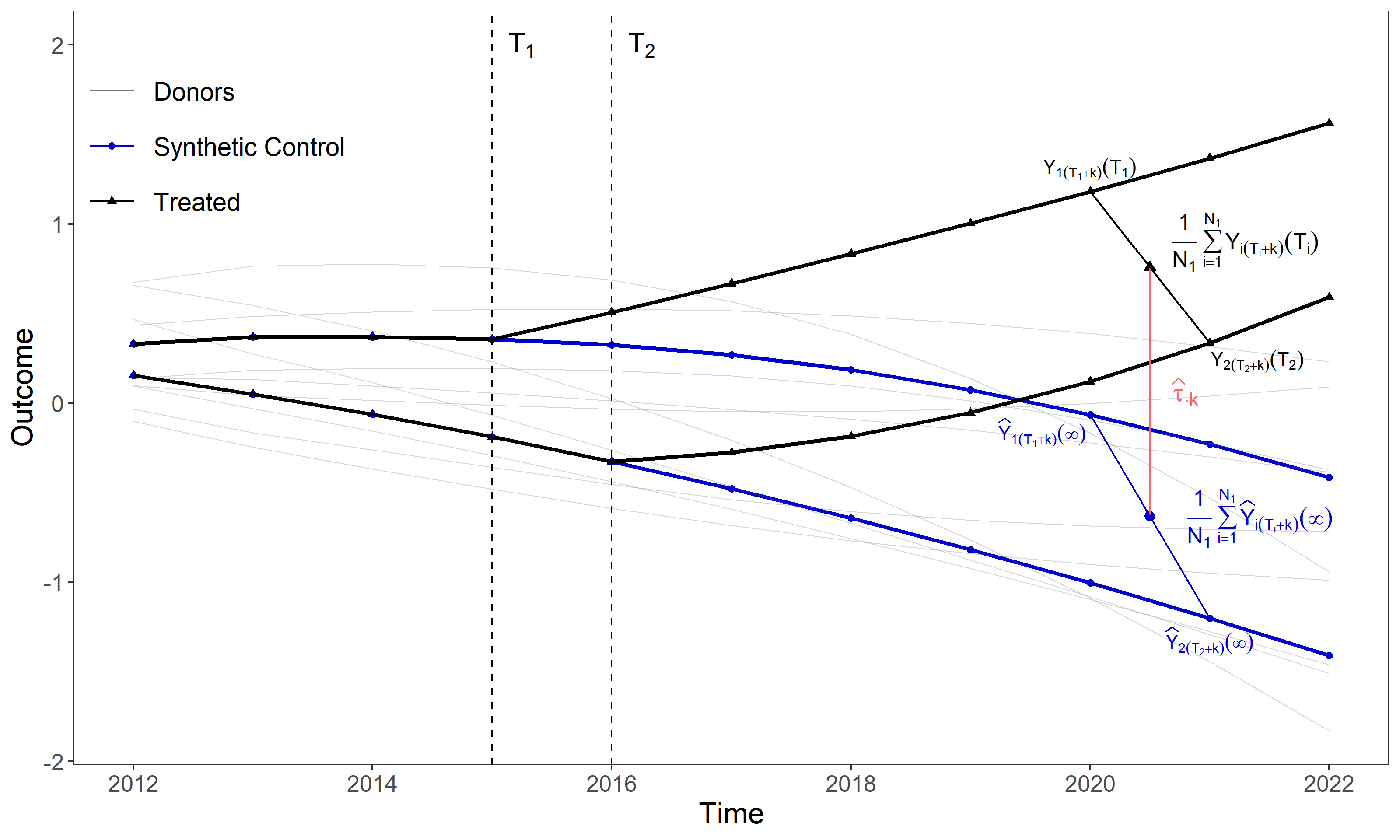
Figure 4: Graphical illustration of the average treatment effect on all treated after $k$ periods $\widehat{\tau}_{\cdot k}$.

Notes: The black lines display the times series of the treated units’ outcome, whereas the blurred gray lines portray the same variable for the donor units. The blue lines are the synthetic controls constructed out of the donor units using a simplex-type constraint. The largest black triangle represents the average of the treated units’ outcomes $k$ periods after treatment, with $k$ set to 5. Similarly, the largest blue circle is the average of the synthetic controls $k$ periods after treatment. The pink vertical line represents the quantity $\widehat{\tau}_{\cdot k,s_{0}}$ described in Example 3.4.

As pointed out by Ben-Michael, Feller and Rothstein (2022), with multiple treated units, the SC weights could be constructed in two ways: (i) optimizing the separate fit for each treated unit; (ii) optimizing the pooled fit for the average of the treated units. These ideas can be accommodated by choosing a proper weighting matrix $\mathbf{V}$. For example, taking $\mathbf{V}=\mathbf{I}_{T_{0}MN_{1}}$ yields

$$\widehat{\bm{\beta}}=\underset{\mathbf{w}\in\mathcal{W},\mathbf{r}\in\mathcal{R}}{\arg\min}\sum_{i=1}^{N_{1}}\sum_{l=1}^{M}\sum_{t=1}^{T_{0}}\Big{(}a_{t,l}^{[i]}-\mathbf{b}_{t,l}^{[i]\prime}\mathbf{w}_{l}^{[i]}-\mathbf{c}_{t,l}^{[i]\prime}\mathbf{r}_{l}^{[i]}\Big{)}^{2},$$

where $\mathbf{B}_{l}^{[i]}:=(\mathbf{b}_{1,l}^{[i]},\cdots,\mathbf{b}_{T_{0},l}^{[i]})^{\prime}$ is the $l$th feature of the $J$ control units in the donor pool, and $\mathbf{C}_{l}^{[i]}:=(\mathbf{c}_{1,l}^{[i]},\cdots,\mathbf{c}_{T_{0},l}^{[i]})^{\prime}$ is the additional $K$ variables used to predict $\mathbf{A}_{l}^{[i]}$. The objective above is equivalent to minimizing the sum of squared errors of the pre-treatment fit for each treated unit and thus is termed “separate fit”.

By contrast, consider the following weighting matrix:

$$\mathbf{V}=\frac{1}{N_{1}^{2}}\bm{1}_{N_{1}}\bm{1}_{N_{1}}^{\prime}\otimes\mathbf{I}_{T_{0}M}$$

where $\otimes$ denotes the Kronecker product operator. Then,

$$\widehat{\bm{\beta}}=\underset{\mathbf{w}\in\mathcal{W},\mathbf{r}\in\mathcal{R}}{\arg\min}\sum_{l=1}^{M}\sum_{t=1}^{T_{0}}\bigg{[}\frac{1}{N_{1}}\sum_{i=1}^{N_{1}}\Big{(}a_{t,l}^{[i]}-\mathbf{b}_{t,l}^{[i]\prime}\mathbf{w}^{[i]}-\mathbf{c}_{t,l}^{[i]\prime}\mathbf{r}_{l}^{[i]}\Big{)}\bigg{]}^{2}.$$

In this case, the goal is to minimize the sum of squared averaged errors across all treated units, which is usually termed “pooled fit”.

To simplify the exposition, we assume that the number of pre-treatment periods $T_{0}$ and the number of control units $J$ do not vary when we match on features of different treated units. This accommodates the common practice of using data in all periods before the first unit is treated (i.e., $T_{0}=T_{1}-1$) and taking all units that are never treated as donors (i.e., $J=N_{0}$). However, our setup is general enough to allow for more flexible choices of pre-treatment periods and donor pools that are heterogeneous across different treated units, at the cost of additional cumbersome notation. Selecting the appropriate donor pool for each treatment unit in practice can be done taking into account the causal predictand of interest.

4 Prediction Intervals

Our goal is to use our generic synthetic control framework to construct prediction intervals for the various treatment effects defined in Section 3. Suppose that $\mathbf{A}$, $\mathbf{B}$, and $\mathbf{C}$ introduced previously are random quantities defined on a probability space $(\Omega,\mathscr{F},\mathbb{P})$, and $\mathscr{H}\subseteq\mathscr{F}$ is a sub-$\sigma$-field. For some $\alpha,\pi\in(0,1)$, we say a random interval $\mathcal{I}$ is an $(\alpha,\pi)$-valid $\mathscr{H}$-conditional prediction interval for a causal predictand $\tau$ if

$$\mathbb{P}\Big{\{}\mathbb{P}\big{[}\tau\in\mathcal{I}\,\big{|}\,\mathscr{H}\big{]}\geq 1-\alpha\Big{\}}\geq 1-\pi,$$ (4.1)

where $\tau$ can be thought of as any of the treatment effects defined in Section 3.

If $\mathscr{H}$ is the trivial $\sigma$-field over $\Omega$, then $\mathcal{I}$ reduces to an unconditional prediction interval for $\tau$. In the general case, the prediction interval $\mathcal{I}$ is $\mathscr{H}$-conditionally $(\alpha,\pi)$-valid: the conditional coverage probability of $\mathcal{I}$ for $\tau$ is at least $(1-\alpha)$, which holds with probability over $\mathscr{H}$ at least $(1-\pi)$. In practice, $(1-\alpha)$ is a desired coverage level chosen by users, say $95\%$, and $\pi$ is a “small” number that depends on the sample size and typically goes to zero in some asymptotic sense. In this paper, all results are valid for all $T_{0}$ large enough, with the associated probability loss $\pi$ characterized precisely. Thus, we say that the conditional coverage of the prediction interval $\mathcal{I}$ is at least $(1-\alpha)$ with high probability, or that the conditional prediction interval offers finite-sample probability guarantees. Our results imply that $\pi\to 0$ as $T_{0}\to\infty$, but no limits or asymptotic arguments are used in this paper.

Generally, the choice of the conditioning set $\mathscr{H}$ determines the uncertainty that would not be taken into account by the prediction intervals. We consider prediction intervals conditional on all control units as well as on the other predictors used to construct the SC prediction. That is, $\mathscr{H}=\{\mathbf{B},\mathbf{C},\mathbf{p}_{\tau}\}$. Therefore, the uncertainty to be characterized arises from the treated units only. Define the target quantity of the SC weights (conditional on $\mathscr{H}$) that is analogous to (3.1):

$$\bm{\beta}_{0}:=(\mathbf{w}_{0}^{\prime},\,\mathbf{r}_{0}^{\prime})^{\prime}=\underset{\mathbf{w}\in\mathcal{W},\,\mathbf{r}\in\mathcal{R}}{\arg\min}\;\mathbb{E}\Big{[}(\mathbf{A}-\mathbf{B}\mathbf{w}-\mathbf{C}\mathbf{r})^{\prime}\mathbf{V}(\mathbf{A}-\mathbf{B}\mathbf{w}-\mathbf{C}\mathbf{r})\Big{|}\mathscr{H}\Big{]}.$$ (4.2)

Thus, we can write

$$\mathbf{A}=\mathbf{B}\mathbf{w}_{0}+\mathbf{C}\mathbf{r}_{0}+\mathbf{U},\qquad\mathbf{w}_{0}\in\mathcal{W},\qquad\mathbf{r}_{0}\in\mathcal{R},$$ (4.3)

where $\mathbf{U}=(\mathbf{u}^{[1]\prime},\cdots,\mathbf{u}^{[N_{1}]\prime})^{\prime}\in\mathbb{R}^{T_{0}MN_{1}}$ is the corresponding pseudo-true residual relative to the $\sigma$-field $\mathscr{H}$. Each $\mathbf{u}^{[i]}=(u_{1,1}^{[i]},\cdots,u_{T_{0},1}^{[i]},\cdots,u_{1,M}^{[i]},\cdots,u_{T_{0},M}^{[i]})^{\prime}\in\mathbb{R}^{T_{0}M}$ is the pseudo-true residual from the $M$ equations (corresponding to the $M$ features) of the treated unit $i$. Given the pseudo-true value $\bm{\beta}_{0}$ and a desired causal predictand $\tau$, we have the following decomposition of the predicted effect $\widehat{\tau}$:

$$\widehat{\tau}-\tau\equiv-\mathbf{p}_{\tau}^{\prime}(\widehat{\bm{\beta}}-\bm{\beta}_{0})+e_{\tau},$$

where $\mathbf{p}_{\tau}^{\prime}(\widehat{\bm{\beta}}-\bm{\beta}_{0})$ captures the in-sample uncertainty from the SC weights construction using pre-treatment information, and $e_{\tau}$ captures the out-of-sample uncertainty from the stochastic error in one or a few post-treatment periods. Notice that in-sample uncertainty quantification is necessary in this scenario since the conditioning set $\mathscr{H}\supseteq\{\mathbf{B},\mathbf{C}\}$, but $\mathscr{H}\not\ni\mathbf{A}$.

To construct prediction intervals for a causal predictand $\tau$, we propose to find constants $M_{1,\mathtt{L}}$, $M_{1,\mathtt{U}}$, $M_{2,\mathtt{L}}$ and $M_{2,\mathtt{U}}$, possibly depending on $\alpha_{1},\alpha_{2},\pi_{1},\pi_{2}\in(0,1)$ such that

$$\mathbb{P}\Big{\{}\mathbb{P}\big{[}M_{1,\mathtt{L}}\leq\mathbf{p}_{\tau}^{\prime}( \widehat{\bm{\beta}}-\bm{\beta}_{0}) \leq M_{1,\mathtt{U}}\; \big{|}\;\mathscr{H}\big{]}\geq 1-\alpha_{1}\Big{\}}\geq 1-\pi_{1},\qquad\text{and}$$

$$\mathbb{P}\Big{\{}\mathbb{P}\big{[}M_{2,\mathtt{L}}\leq e_{\tau} \leq M_{2,\mathtt{U}}\; \big{|}\;\mathscr{H}\big{]}\geq 1-\alpha_{2}\Big{\}}\geq 1-\pi_{2},$$

which suffices to guarantee

$$\mathbb{P}\Big{\{}\mathbb{P}\big{[}\widehat{\tau}+M_{1,\mathtt{L}}-M_{2,\mathtt{U}}\leq\tau\leq\widehat{\tau}+M_{1,\mathtt{U}}-M_{2,\mathtt{L}}\big{|}\mathscr{H}\big{]}\geq 1-\alpha_{1}-\alpha_{2}\Big{\}}\geq 1-\pi_{1}-\pi_{2},$$

that is, the prediction interval $\mathcal{I}=[\widehat{\tau}+M_{1,\mathtt{L}}-M_{2,\mathtt{U}},\,\widehat{\tau}+M_{1,\mathtt{U}}-M_{2,\mathtt{L}}]$ achieves $(1-\alpha_{1}-\alpha_{2})$ $\mathscr{H}$-conditional coverage probability, which holds with probability at least $1-\pi_{1}-\pi_{2}$ over $\mathscr{H}$, as defined in (4.1).

In-sample uncertainty. We propose a simulation-based strategy to bound the in-sample error $\mathbf{p}_{\tau}^{\prime}(\bm{\beta}_{0}-\widehat{\bm{\beta}})$. Let $\mathbf{Z}=(\mathbf{B},\mathbf{C})$ and $d=(J+KM)N_{1}$. Using (3.1) and (4.2), we obtain the following optimization problem characterizing the centered synthetic control weights predictor:

$$\widehat{\bm{\beta}}-\bm{\beta}_{0}=\operatorname*{arg\,min}_{\bm{\beta}-\bm{\beta}_{0}\in\Delta}\Big{\{}(\bm{\beta}-\bm{\beta}_{0})^{\prime}\widehat{\mathbf{Q}}(\bm{\beta}-\bm{\beta}_{0})-2\widehat{\bm{\gamma}}^{\prime}(\bm{\beta}-\bm{\beta}_{0})\Big{\}},$$

where $\widehat{\mathbf{Q}}=\mathbf{Z}^{\prime}\mathbf{V}\mathbf{Z}$, $\widehat{\bm{\gamma}}^{\prime}=\mathbf{U}^{\prime}\mathbf{V}\mathbf{Z}$, and $\Delta=\{\bm{\beta}-\bm{\beta}_{0}\in\mathbb{R}^{d}:\bm{\beta}\in\mathcal{W}\times\mathcal{R}\}$. We assume that the constraint sets $\mathcal{W}$ and $\mathcal{R}$ are convex throughout.

Let $\bm{\gamma}:=\mathbb{E}[\widehat{\bm{\gamma}}|\mathscr{H}]$, which is not necessarily equal to $\mathbf{0}$. By optimality of $\widehat{\bm{\beta}}$ and the convexity of $\mathcal{W}$ and $\mathcal{R}$, it can be shown that $\widehat{\bm{\beta}}$ has to satisfy $\widehat{\bm{\beta}}-\bm{\beta}_{0}\in\Delta$ and $(\widehat{\bm{\beta}}-\bm{\beta}_{0})^{\prime}\widehat{\mathbf{Q}}(\widehat{\bm{\beta}}-\bm{\beta}_{0})-2(\widehat{\bm{\gamma}}-\bm{\gamma})^{\prime}(\widehat{\bm{\beta}}-\bm{\beta}_{0})\leq 0$. Thus, the minimum and the maximum of $\mathbf{p}_{\tau}^{\prime}(\bm{\beta}-\bm{\beta}_{0})$ over the set of $\bm{\beta}$ satisfying these restrictions are lower and upper bounds on the in-sample error $\mathbf{p}_{\tau}^{\prime}(\widehat{\bm{\beta}}-\bm{\beta}_{0})$. Conditional on $\mathscr{H}$, the uncertainty of these (stochastic) bounds comes from $\widehat{\bm{\gamma}}$ only. We can employ a normal distributional approximation of $\widehat{\bm{\gamma}}$ and set $M_{1,\mathtt{L}}=\mathfrak{c}_{\mathtt{L}}(\alpha_{1}/2)$ and $M_{1,\mathtt{U}}=\mathfrak{c}_{\mathtt{U}}(1-\alpha_{1}/2)$ where

$$\mathfrak{c}_{\mathtt{L}}(\alpha_{1}/2):=(\alpha_{1}/2)\text{-quantile of }\inf\{\mathbf{p}_{\tau}^{\prime}\bm{\delta}:\bm{\delta}\in\mathcal{M}_{\mathbf{G}}\}\quad\text{and}$$

$$\mathfrak{c}_{\mathtt{U}}(1-\alpha_{1}/2):=(1-\alpha_{1}/2)\text{-quantile of }\sup\{\mathbf{p}_{\tau}^{\prime}\bm{\delta}:\bm{\delta}\in\mathcal{M}_{\mathbf{G}}\}$$

conditional on $\mathscr{H}$, with $\mathcal{M}_{\mathbf{G}}=\{\bm{\delta}\in\Delta:\bm{\delta}^{\prime}\widehat{\mathbf{Q}}\bm{\delta}-2\mathbf{G}^{\prime}\bm{\delta}\leq 0\}$, $\mathbf{G}|\mathscr{H}\thicksim\mathsf{N}(\mathbf{0},\bm{\Sigma})$ and $\bm{\Sigma}=\mathbb{V}[\widehat{\bm{\gamma}}|\mathscr{H}]$.

However, $\mathfrak{c}_{\mathtt{L}}(\alpha_{1}/2)$ and $\mathfrak{c}_{\mathtt{U}}(1-\alpha_{1}/2)$ cannot be directly used because they still rely on the infeasible normalized constraint set $\Delta$ and the unknown covariance matrix $\bm{\Sigma}$. We thus propose a feasible simulation-based strategy allowing for possibly nonlinear constraints, where we replace unknown quantities by plug-in approximations thereof.

First, we need a feasible constraint set $\Delta^{\star}$ used in simulation. Specifically, define the distance between a point $\mathbf{a}\in\mathbb{R}^{d}$ and a set $\Lambda\subseteq\mathbb{R}^{d}$ by $\mathrm{dist}(\mathbf{a},\Lambda)=\inf_{\lambda\in\Lambda}\|\mathbf{a}-\bm{\lambda}\|$, where $\|\cdot\|$ is a generic $\ell_{p}$ vector norm on $\mathbb{R}^{d}$ with $p\geq 1$ (e.g., Euclidean norm or $\ell_{1}$ norm). Intuitively, we require that every point in the original infeasible constraint set $\Delta$ be close to the feasible constraint set $\Delta^{\star}$ in simulation. Consequently, searching for an upper (or lower) bound within the infeasible set $\Delta$ can be replaced with doing so within the feasible set $\Delta^{\star}$. This requirement will be formalized as condition (iii) in Theorem 1 below. A proposed strategy for constructing $\Delta^{\star}$ is described in (4.6), and more implementation details are discussed in Section 5.2.

Second, we need an estimator $\widehat{\bm{\Sigma}}$ of the covariance matrix $\bm{\Sigma}$. A variety of well-established heteroskedasticity/serial-correlation-robust estimators can be used. We require $\widehat{\bm{\Sigma}}$ to be a “good” approximation of $\bm{\Sigma}$ in the sense of condition (iv) in Theorem 1 below. This allows us to approximate the infeasible normal distribution $\mathsf{N}(\bm{0},\bm{\Sigma})$ by $\mathsf{N}(\bm{0},\widehat{\bm{\Sigma}})$, which can be simulated using the data.

Once $\Delta^{\star}$ and $\widehat{\bm{\Sigma}}$ are available, we can simply draw random vectors from $\mathsf{N}(\bm{0},\widehat{\bm{\Sigma}})$ conditional on the data, and then set

$$M_{1,\mathtt{L}}=\mathfrak{c}_{\mathtt{L}}^{\star}(\alpha_{1}/2)\quad\text{and}\quad M_{1,\mathtt{U}}=\mathfrak{c}_{\mathtt{U}}^{\star}(1-\alpha_{1}/2)$$ (4.4)

where

$$\mathfrak{c}_{\mathtt{L}}^{\star}(\alpha_{1}/2):=(\alpha_{1}/2)\text{-quantile of }\inf\{\mathbf{p}_{\tau}^{\prime}\bm{\delta}:\bm{\delta}\in\mathcal{M}_{\mathbf{G}}^{\star}\}\quad\text{and}$$

$$\mathfrak{c}_{\mathtt{U}}^{\star}(1-\alpha_{1}/2):=(1-\alpha_{1}/2)\text{-quantile of }\sup\{\mathbf{p}_{\tau}^{\prime}\bm{\delta}:\bm{\delta}\in\mathcal{M}_{\mathbf{G}}^{\star}\}$$

conditional on the data, $\mathcal{M}_{\mathbf{G}}^{\star}=\{\bm{\delta}\in\Delta^{\star}:\;\bm{\delta}^{\prime}\widehat{\mathbf{Q}}\bm{\delta}-2(\mathbf{G}^{\star})^{\prime}\bm{\delta}\leq 0\}$, and $\mathbf{G}^{\star}|\mathsf{Data}\sim\mathsf{N}(\bm{0},\widehat{\bm{\Sigma}})$.

For example, our main empirical results in Section 6 employ an L1-L2 constrained synthetic control prediction (non-linear constraints) and carefully chosen plug-in approximations $(\Delta^{\star},\widehat{\bm{\Sigma}})$ (described precisely below), which exhibits good performance in finite samples. Validity of the resulting non-asymptotic prediction intervals is new to the literature because prior results covered only linear constraints (see Theorem 1) and, in particular, did not provide a principled $\Delta^{\star}$ (see Lemma 1).

Out-of-sample uncertainty. To bound the out-of-sample error $e_{\tau}$, we propose an easy-to-implement approach based on non-asymptotic concentration inequalities. Specifically, assume that $e_{\tau}-\mathbb{E}[e_{\tau}|\mathscr{H}]$ is conditional-on-$\mathscr{H}$ sub-Gaussian with parameter $\sigma_{\mathscr{H}}$. Then for any $\varepsilon>0$,

$$\mathbb{P}\Big{(}|e_{\tau}-\mathbb{E}[e_{\tau}|\mathscr{H}]|\geq\varepsilon\Big{|}\mathscr{H}\Big{)}\leq 2\exp\Big{(}-\frac{\varepsilon^{2}}{2\sigma_{\mathscr{H}}^{2}}\Big{)}.$$

Consequently, we set

$$M_{2,\mathtt{L}}=\mathbb{E}[e_{\tau}|\mathscr{H}]-\sqrt{2\sigma_{\mathscr{H}}^{2}\log(2/\alpha_{2})}\qquad\text{and}\qquad M_{2,\mathtt{U}}=\mathbb{E}[e_{\tau}|\mathscr{H}]+\sqrt{2\sigma_{\mathscr{H}}^{2}\log(2/\alpha_{2})},$$ (4.5)

which yields a prediction interval $[M_{2,\mathtt{L}},M_{2,\mathtt{U}}]$ that covers $e_{T_{i}+k}^{[i]}$ with at least $(1-\alpha_{2})$ conditional coverage probability. We emphasize that the sub-Gaussianity assumption is one of many possibilities. The above strategy could applied using other concentration inequalities requiring weaker moment conditions, though the resulting prediction intervals may be wider.

As discussed in the examples below, the generic out-of-sample error $e_{\tau}$ associated with some treatment effect $\tau$ is typically a linear combination of individual error terms $e_{t}^{[i]}=Y_{it}(\infty)-\mathbf{p}_{t}^{[i]\prime}\bm{\beta}_{0}$ in the post-treatment period, and the sub-Gaussianity of $e_{\tau}$ is implied by assuming $e_{t}^{[i]}$ is sub-Gaussian. In practice, one could first construct pre-treatment residuals $\widehat{e}_{t}^{[i]}=Y_{it}(\infty)-\mathbf{p}_{t}^{[i]\prime}\widehat{\bm{\beta}}^{[i]}$, $t=1,\cdots,T_{0}$, and estimate the conditional moments of $e_{t}^{[i]}$ employing various parametric or nonparametric regression of $\widehat{e}_{t}^{[i]}$. Such estimates can then be translated into the necessary estimates of $\mathbb{E}[e_{\tau}|\mathscr{H}]$ and $\sigma_{\mathscr{H}}^{2}$ for constructing $M_{2,\mathtt{L}}$ and $M_{2,\mathtt{U}}$. The unknown conditional moments could also be set using external information, or tabulated across different values to assess the sensitivity of the resulting prediction intervals. See Cattaneo, Feng, Palomba and Titiunik (2023) for more implementation details.

Example 4.1 (Individual Treatment Effect, $\tau_{ik}$, continued).

For the causal predictand $\tau_{ik}$, the out-of-sample error is given by

$$e_{\tau_{ik}}=Y_{i(T_{i}+k)}(\infty)-\mathbf{p}_{T_{i}+k}^{[i]\prime}\bm{\beta}_{0}=e_{T_{i}+k}^{[i]},$$

If we assume $e_{t}^{[i]}-\mathbb{E}[e_{t}^{[i]}|\mathscr{H}]$ is sub-Gaussian conditional on $\mathscr{H}$, then the strategy outlined above can be applied.

Example 4.2 (Average Post-Treatment Effect, $\tau_{i\cdot}$, continued).

For the causal predictand $\tau_{i\cdot}$, the out-of-sample error is given by

$$e_{\tau_{i\cdot}}:=\frac{1}{T-T_{i}+1}\sum_{t=T_{i}}^{T}\Big{(}Y_{it}(\infty)-\mathbf{p}_{t}^{[i]\prime}\bm{\beta}_{0}^{[i]}\Big{)}=\frac{1}{T-T_{i}+1}\sum_{t=T_{i}}^{T}e_{t}^{[i]}.$$

The approach outlined above can still be applied to $e_{\tau_{i\cdot}}$. For example, if $e_{t}^{[i]}-\mathbb{E}[e_{t}^{[i]}|\mathscr{H}]$ is conditional-on-$\mathscr{H}$ sub-Gaussian with parameter $\sigma_{\mathscr{H},t}>0$ for $t=T_{i},\cdots,T$, it can be shown that $e_{\tau_{i\cdot}}$, as the average of $e_{t}^{[i]}$ across time, satisfies that for any $\varepsilon>0$,

$$\mathbb{P}(|e_{\tau_{i\cdot}}-\mathbb{E}[e_{\tau_{i\cdot}}|\mathscr{H}]|\geq\varepsilon|\mathscr{H})\leq 2\exp\Big{(}-\varepsilon^{2}/(2\bar{\sigma}_{\mathscr{H}}^{2})\Big{)},\quad\bar{\sigma}_{\mathscr{H}}=\frac{1}{T-T_{i}+1}\sum_{t=T_{i}}^{T}\sigma_{\mathscr{H},t}.$$

This inequality holds regardless of the dependence structure of $e_{t}^{[i]}$. If $e_{t}^{[i]}$ is independent over $t$, the above result can be improved:

$$\mathbb{P}(|e_{\tau_{i\cdot}}-\mathbb{E}[e_{\tau_{i\cdot}}|\mathscr{H}]|\geq\varepsilon|\mathscr{H})\leq 2\exp\Big{(}-\varepsilon^{2}/(2\tilde{\sigma}_{\mathscr{H}}^{2})\Big{)},\quad\tilde{\sigma}_{\mathscr{H}}=\frac{1}{T-T_{i}+1}\bigg{(}\sum_{t=T_{i}}^{T}\sigma^{2}_{\mathscr{H},t}\bigg{)}^{1/2}.$$

In this case, one can characterize each $\sigma_{\mathscr{H},t}$, $t=T_{i},\cdots,T$, and use the idea outlined above to construct bounds on $e_{\tau_{i\cdot}}$.

Alternatively, one could construct a pre-treatment sequence of errors that is analogous to $e_{\tau_{i\cdot}}$:

$$\tilde{e}_{t}^{[i]}:=\frac{1}{T-T_{i}+1}\sum_{t=\ell}^{\ell+T-T_{i}}e_{t}^{[i]},\quad 1\leq\ell\leq 2T_{i}-T-1,$$

and then apply the strategy outlined before to this new sequence of errors, which requires characterizing the (conditional) moments of $\tilde{e}_{t}^{[i]}$. One caveat is that by construction, $\tilde{e}_{t}^{[i]}$ could have a different dependence structure from the original sequence $e_{t}^{[i]}$. For example, even if $e_{t}^{[i]}$ is independent over $t$ conditional on $\mathscr{H}$, $\tilde{e}_{t}^{[i]}$ would be $(T-T_{i}+1)$-dependent conditional on $\mathscr{H}$ in general, that is, $\tilde{e}_{t}^{[i]}$ is independent of $\tilde{e}_{t+\ell}^{[i]}$ conditional on $\mathscr{H}$ if $\ell\geq T-T_{i}+1$.

Example 4.3 (Average Treatment Effect on the Treated at $s_{0}$ after $k$ Periods, $\tau_{\cdot k,s_{0}}$, continued).

In this scenario, the out-of-sample error is given by

$$e_{\tau_{\cdot k,s_{0}}}:=\frac{1}{n_{s_{0}}}\sum_{i:T_{i}=s_{0}}\Big{(}Y_{i(s_{0}+k)}(\infty)-\mathbf{p}_{s_{0}+k}^{[i]\prime}\bm{\beta}_{0}^{[i]}\Big{)}=\frac{1}{n_{s_{0}}}\sum_{i:T_{i}=s_{0}}e_{s_{0}+k}^{[i]}.$$

The out-of-sample error above is similar to that defined in Example 4.2 except that $e_{\tau_{\cdot k,s_{0}}}$ is a cross-sectional average of $e_{t}^{[i]}$ rather than a time-series average. The uncertainty quantification strategy outlined in Example 4.2 can still be applied, with the caveat that it is uncommon in SC analysis to assume $e_{t}^{[i]}$ is stationary and/or independent over $i$. By contrast, it is reasonable to assume $e_{t}^{[i]}$ is stationary and/or independent (at least weakly dependent) over time.

Example 4.4 (Average Treatment Effect on all Treated after $k$ Periods, $\tau_{\cdot k}$, continued).

In this scenario, the out-of-sample error is given by

$$e_{\tau_{\cdot k}}:=\frac{1}{N_{1}}\sum_{i=1}^{N_{1}}\Big{(}Y_{i(T_{i}+k)}(\infty)-\mathbf{p}_{T_{i}+k}^{[i]\prime}\bm{\beta}_{0}^{[i]}\Big{)}=\frac{1}{N_{1}}\sum_{i=1}^{N_{1}}e_{T_{i}+k}^{[i]}.$$

Since the adoption time $T_{i}$ may be heterogeneous across $i$, $e_{\tau_{\cdot k}}$ is an average of the individual errors $e_{t}^{[i]}$ of different units in different periods. Again, one can characterize the (conditional) moments of each $e_{t}^{[i]}$ and use the concentration-inequality-based approach to bound $e_{\tau_{\cdot k}}$. By contrast, it would be difficult to implement the other strategy outlined in Example 4.2 that relies on constructed pre-treatment averaged errors analogous to $e_{\tau_{\cdot k}}$, since such averages may include errors that are far away in time and their dependence on $\mathscr{H}$ may be very complex.

In addition to the concentration-based approach described above, other strategies, including location-scale models and quantile regression, were proposed in Cattaneo, Feng and Titiunik (2021) for out-of-sample uncertainty quantification. We briefly review them in Supplemental Appendix S.1.1.

Main theorem. We present our main theorem, which shows that the prediction interval constructed above achieves approximately $(1-\alpha_{1}-\alpha_{2})$ conditional coverage probability, which holds with high probability on $\mathscr{H}$. We use $\|\cdot\|_{*}$ to denote the dual norm of $\|\cdot\|$ on $\mathbb{R}^{d}$, use $\|\cdot\|_{\mathtt{F}}$ to denote the Frobenius matrix norm, and use $\mathcal{B}(\mathbf{0},\varepsilon)$ to denote an $\varepsilon$-neighborhood around zero for some $\varepsilon>0$.

Theorem 1.

Assume $\mathcal{W}$ and $\mathcal{R}$ are convex, $\widehat{\bm{\beta}}$ in (3.1) and $\bm{\beta}_{0}$ in (4.2) exist, $\mathscr{H}=\sigma(\mathbf{B},\mathbf{C},\mathbf{p}_{\tau})$, and $M_{1,\mathtt{L}}$, $M_{1,\mathtt{U}}$, $M_{2,\mathtt{L}}$ and $M_{2,\mathtt{U}}$ are specified as in (4.4) and (4.5). In addition, for some finite non-negative constants $\epsilon_{\gamma}$, $\pi_{\gamma}$, $\varpi_{\delta}^{\star}$, $\epsilon_{\delta}^{\star}$, $\pi_{\delta}^{\star}$, $\varpi_{\Delta}^{\star}$, $\epsilon_{\Delta}^{\star}$, $\pi_{\Delta}^{\star}$, $\epsilon_{\gamma,1}^{\star}$, $\epsilon_{\gamma,2}^{\star}$ and $\pi_{\gamma}^{\star}$, the following conditions hold:

1. $\mathbb{P}[\mathbb{P}(\mathbf{p}_{\tau}^{\prime}(\widehat{\bm{\beta}}-\bm{\beta}_{0})\in[\mathfrak{c}_{\mathtt{L}}(\alpha_{0}),\mathfrak{c}_{\mathtt{U}}(1-\alpha_{0})]|\mathscr{H})\geq 1-\alpha_{0}-\epsilon_{\gamma}]\geq 1-\pi_{\gamma}$ for any $\alpha_{0}\in(0,1)$;

2. $\mathbb{P}[\mathbb{P}(\sup\{\|\bm{\delta}\|:\bm{\delta}\in\mathcal{M}_{\mathbf{G}}\}\leq\varpi_{\delta}^{\star}|\mathscr{H})\geq 1-\epsilon_{\delta}^{\star}]\geq 1-\pi_{\delta}^{\star}$;

3. $\mathbb{P}[\mathbb{P}(\sup_{\mathbf{a}\in\Delta\cap\mathcal{B}(0,\varpi_{\delta}^{\star})}\mathrm{dist}(\mathbf{a},\Delta^{\star}\cap\mathcal{B}(0,\varepsilon))\leq\varpi_{\Delta}^{\star}\;|\mathscr{H})\geq 1-\epsilon_{\Delta}^{\star}]\geq 1-\pi_{\Delta}^{\star}$;

4. $\mathbb{P}[\mathbb{P}(\|\bm{\Sigma}^{-1/2}\widehat{\bm{\Sigma}}\bm{\Sigma}^{-1/2}-\mathbf{I}_{d}\|_{\mathtt{F}}\leq 2\epsilon_{\gamma,1}^{\star}|\mathscr{H})\geq 1-\epsilon_{\gamma,2}^{\star}]\geq 1-\pi_{\gamma}^{\star}$;

5. $e_{\tau}-\mathbb{E}[e_{\tau}|\mathscr{H}]$ is sub-Gaussian conditional on $\mathscr{H}$ with parameter $\sigma_{\mathscr{H}}$.

Then, for $\epsilon_{\gamma,1}^{\star}\in[0,1/4]$,

$$\mathbb{P}\Big{\{}\mathbb{P}\big{(}\tau\in[\widehat{\tau}+M_{1,\mathtt{L}}-M_{2,\mathtt{U}}-\varepsilon_{\Delta},\;\widehat{\tau}+M_{1,\mathtt{U}}-M_{2,\mathtt{L}}+\varepsilon_{\Delta}]\big{|}\mathscr{H}\big{)}\geq 1-\alpha_{1}-\alpha_{2}-\epsilon\Big{\}}\geq 1-\pi,$$

where $\epsilon=\epsilon_{\gamma}+2\epsilon_{\gamma,1}^{\star}+\epsilon_{\gamma,2}^{\star}+2\epsilon_{\delta}^{\star}+\epsilon_{\Delta}^{\star}$, $\pi=\pi_{\gamma}+\pi_{\gamma}^{\star}+\pi_{\delta}^{\star}+\pi_{\Delta}^{\star}$ and $\varepsilon_{\Delta}=\|\mathbf{p}_{\tau}\|_{*}\varpi_{\Delta}^{\star}$.

Assumptions (i)-(iv) are high-level conditions used for in-sample uncertainty quantification, which can be verified in many practically relevant scenarios. See more detailed discussion in Section 4.1. Condition (v), as we emphasized before, is a moment condition on $e_{\tau}$ that is used to showcase our out-of-sample uncertainty quantification strategy and can be relaxed by utilizing other appropriate concentration inequalities. Moreover, the constant $\varepsilon_{\Delta}$ in the theorem is used to adjust the prediction interval for nonlinear constraints. In many SC applications with linear constraints only (e.g., simplex or lasso constraint), such adjustment is unnecessary and we can set $\varepsilon_{\Delta}=0$. See Section 5.3 for more discussion.

4.1 Discussion of Conditions (i)-(iv)

Theorem 1 relies on the high-level conditions (i)-(iv). We discuss each of them in more detail.

• Condition (i). This condition formalizes the idea of distributional approximation of $\widehat{\bm{\gamma}}-\bm{\gamma}$ by a Gaussian vector $\mathbf{G}$. Lemma S.1 in the Supplemental Appendix verifies (i) by assuming the error term $(u_{t,1}^{[1]},\cdots,u_{t,M}^{[1]},\cdots,u_{t,1}^{[N_{1}]},\cdots,u_{t,M}^{[N_{1}]})^{\prime}$ is independent over $1\leq t\leq T_{0}$ conditional on $\mathscr{H}$. In fact, (i) also holds when the errors are only weakly dependent (e.g., $\beta$-mixing) conditional on $\mathscr{H}$. See more discussion in Section S.2.2 of the Supplemental Appendix. Importantly, the features included in $\mathbf{A}$ and $\mathbf{B}$ could be non-stationary, thus covering the cointegration case which is common in SC applications.

• Condition (ii). This is a mild condition on the concentration of $\bm{\delta}\in\mathcal{M}_{\mathbf{G}}$. The requirement $\bm{\delta}^{\prime}\widehat{\mathbf{Q}}\bm{\delta}-2\mathbf{G}^{\prime}\bm{\delta}\leq 0$ is usually known as the basic inequality in regression analysis (see Chapter 7 of Wainwright (2019) for the example of lasso). The vector $\mathbf{G}$ is (conditional) Gaussian by construction, making condition (ii) easy to verify based on well-known bounds for Gaussian distributions. This condition holds in a variety of empirically relevant settings, including outcomes-only regression with i.i.d. data, multi-equation regression with weakly dependent data, and cointegrated outcomes and features settings.

• Condition (iii). This is a high-level requirement on the “closeness” between $\Delta$ and $\Delta^{\star}$. We propose a strategy for constructing $\Delta^{\star}$ that can be shown to satisfy (iii) if the constraints specified in $\mathcal{W}$ and $\mathcal{R}$ are formed by smooth functions. Suppose that

  $$\mathcal{W}\times\mathcal{R}=\Big{\{}\bm{\beta}\in\mathbb{R}^{d}:\bm{m}_{\mathtt{eq}}(\bm{\beta})=\bm{0},\bm{m}_{\mathtt{in}}(\bm{\beta})\leq\bm{0}\Big{\}},$$

  where $\bm{m}_{\mathtt{eq}}(\cdot)\in\mathbb{R}^{d_{\mathtt{eq}}}$ and $\bm{m}_{\mathtt{in}}(\cdot)\in\mathbb{R}^{d_{\mathtt{in}}}$ and $d_{\mathtt{eq}}$ and $d_{\mathtt{in}}$ denote the number of equality and inequality constraints in $\mathcal{W}\times\mathcal{R},$ respectively. Let the $j$th constraint in $\bm{m}_{\mathtt{in}}(\cdot)$ be $m_{\mathtt{in},j}(\cdot)$. Given tuning parameters $\varrho_{j}>0$, $j=1,\cdots,d_{\mathtt{in}}$, let $\mathcal{A}=\{j_{1},\cdots,j_{k}\}$ denote the set of indices for the inequality constraints such that $m_{\mathtt{in},j}(\widehat{\bm{\beta}})>-\varrho_{j}$. Then define

  $$\small\Delta^{\star}=\Big{\{}\bm{\beta}-\widehat{\bm{\beta}}:\bm{m}_{\mathtt{eq}}(\bm{\beta})=\bm{0},m_{\mathtt{in},j}(\bm{\beta})\leq m_{\mathtt{in},j}(\widehat{\bm{\beta}})\text{ for }j\in\mathcal{A},m_{\mathtt{in},l}(\bm{\beta})\leq\bm{0}\text{ for }l\notin\mathcal{A}\Big{\}}.$$ (4.6)

  The following lemma verifies condition (iii) for this $\Delta^{\star}$. We use $s_{\min}(\mathbf{M})$ to denote the minimum singular value of a matrix $\mathbf{M}$.

  Lemma 1.

  Let $\|\cdot\|$ be the Euclidean norm for vectors and the spectral norm for matrices. Assume that with probability over $\mathscr{H}$ at least $1-\pi_{\Delta}^{\star}$, the following conditions hold: (i) $\mathbb{P}(\|\widehat{\bm{\beta}}-\bm{\beta}_{0}\|\leq\varpi_{\delta}^{\star}|\mathscr{H})\geq 1-\epsilon_{\Delta}^{\star}$; (ii) $\bm{m}(\cdot)=(\bm{m}_{\mathtt{eq}}(\cdot)^{\prime},\bm{m}_{\mathtt{in}}(\cdot)^{\prime})^{\prime}$ is twice continuously differentiable on $\mathcal{B}(\bm{\beta}_{0},\varpi_{\delta}^{\star})$ with $\inf_{\bm{\beta}\in\mathcal{B}(\bm{\beta}_{0},\varpi_{\delta}^{\star})}s_{\min}(\frac{\partial}{\partial\bm{\beta}^{\prime}}\bm{m}(\bm{\beta}))\geq c_{\min}$ for some constant $c_{\min}>0$; and (iii) for all $1\leq j\leq d_{\mathtt{in}}$, $\varrho_{j}\in(\mathfrak{c}\varpi_{\delta}^{\star},\;|m_{\mathtt{in},j}(\bm{\beta}_{0})|-\mathfrak{c}\varpi_{\delta}^{\star})$ for some $\mathfrak{c}>0$ specified in the proof. Then, for $\Delta^{\star}$ defined in (4.6), condition (iii) in Theorem 1 holds with $\varpi_{\Delta}^{\star}=\mathfrak{C}(\varpi_{\delta}^{\star})^{2}$ for some constant $\mathfrak{C}>0$.

  In this lemma, the tuning parameters $\varrho_{j}$ are introduced to guarantee that with high probability, we can correctly differentiate the binding inequality constraints from the other non-binding ones. In Section 5 below, we provide more practical details about choosing $\varrho_{j}$. Also, the concentration requirement for $\widehat{\bm{\beta}}$ specified in this lemma is usually mild. Since $\widehat{\bm{\beta}}$ satisfies the basic inequality $(\widehat{\bm{\beta}}-\bm{\beta}_{0})^{\prime}\widehat{\mathbf{Q}}(\widehat{\bm{\beta}}-\bm{\beta}_{0})-2(\widehat{\bm{\gamma}}-\bm{\gamma})^{\prime}(\widehat{\bm{\beta}}-\bm{\beta}_{0})\leq 0$, the concentration of $\widehat{\bm{\beta}}$ can be shown by combining a distributional approximation of $\widehat{\bm{\gamma}}-\bm{\gamma}$ by a Gaussian vector $\mathbf{G}$ and the idea outlined in the previous discussion about condition (ii).

• Condition (iv). This is a requirement that $\widehat{\bm{\Sigma}}$ be a “good” approximation of the unknown covariance matrix $\bm{\Sigma}$. Many standard covariance estimation strategies such as the family of well-known heteroskedasticity-consistent estimators can be utilized.

4.2 Simultaneous Prediction Intervals

So far we have focused on constructing prediction intervals that have high coverage of the desired treatment effects, in particular, the individual treatment effect in each post-treatment period. In some applications, it might be appealing to construct prediction intervals that have high simultaneous coverage in multiple post-treatment periods, usually termed simultaneous prediction intervals in the literature. They can be employed to test, for example, whether the largest (or smallest) treatment effect across different periods is significantly different from zero.

Specifically, for a particular treated unit $1\leq i\leq N_{1}$, we aim to construct a sequence of intervals $\mathcal{I}_{k}$ for $0\leq k\leq L$ for some $L\leq T-T_{i}$ such that

$$\mathbb{P}\Big{\{}\mathbb{P}\big{[}\tau_{ik}\in\mathcal{I}_{k},\text{ for all }0\leq k\leq L\,\big{|}\,\mathscr{H}\big{]}\geq 1-\alpha\Big{\}}\geq 1-\pi.$$

As described before, the uncertainty of the predicted individual treatment effect $\widehat{\tau}_{ik}$ comes from the in-sample error $\mathbf{p}_{\tau_{ik}}^{\prime}(\widehat{\bm{\beta}}-\bm{\beta}_{0})$ and the out-of-sample error $e_{T_{i}+k}^{[i]}$.

Regarding the in-sample error, the following is an immediate generalization of the prediction interval described in (4.4), which enjoys simultaneous coverage in multiple periods. If the constraints imposed in $\Delta$ are linear (such as simplex and lasso constraints), set

$$M_{1,\mathtt{L}}:=(\alpha_{1}/2)\text{-quantile of }\inf\,\Big{\{}\mathbf{p}_{\tau_{ik}}^{\prime}\bm{\delta}:\;\bm{\delta}\in\Delta^{\star},\;\ell^{\star}(\bm{\delta})\leq 0,\;0\leq k\leq L\Big{\}}\;\;\text{and}$$

$$M_{1,\mathtt{U}}:=(1-\alpha_{1}/2)\text{-quantile of }\sup\,\Big{\{}\mathbf{p}_{\tau_{ik}}^{\prime}\bm{\delta}:\;\bm{\delta}\in\Delta^{\star},\;\ell^{\star}(\bm{\delta})\leq 0,\;0\leq k\leq L\Big{\}},$$

which guarantees that with high probability,

$$\mathbb{P}\big{[}M_{1,\mathtt{L}}\leq\mathbf{p}_{\tau_{ik}}^{\prime}(\widehat{\bm{\beta}}-\bm{\beta}_{0})\leq M_{1,\mathtt{U}}\text{ for all }0\leq k\leq L\,\big{|}\,\mathscr{H}\big{]}\geq 1-\alpha_{1}.$$

If the constraints imposed in $\Delta$ are nonlinear (such as the ridge-type constraint), further decrease the lower bound $M_{1,\mathtt{L}}$ and increase the upper bound $M_{1,\mathtt{U}}$ defined above by some $\overline{\varepsilon}_{\Delta}$. We regard $\overline{\varepsilon}_{\Delta}$ as a small tuning parameter used to adjust for nonlinear constraints. See more discussion about selecting this parameter in Section 5.3.

Regarding the out-of-sample error, the goal is to find $M_{2,\mathtt{L}}$ and $M_{2,\mathtt{U}}$ such that with high probability,

$$\mathbb{P}\big{[}M_{2,\mathtt{L}}\leq e_{T_{i}+k}^{[i]}\leq M_{2,\mathtt{U}}\text{ for all }0\leq k\leq L\,\big{|}\,\mathscr{H}\big{]}\geq 1-\alpha_{2}.$$

An easy-to-implement strategy analogous to that described in (4.5) is to adjust the intervals based on maximal inequalities. For example, suppose that each $e_{T_{i}+k}^{[i]}-\mathbb{E}[e_{T_{i}+k}^{[i]}|\mathscr{H}]$, $0\leq k\leq L$, is conditional sub-Gaussian with parameter $\sigma_{\mathscr{H},k}$ (but is not necessarily independent over $k$). Then,

$$\mathbb{P}\Big{(}\max_{0\leq k\leq L}|e_{T_{i}+k}^{[i]}-\mathbb{E}[e_{T_{i}+k}^{[i]}|\mathscr{H}]|\geq\varepsilon\Big{|}\mathscr{H}\Big{)}\leq 2\sum_{k=0}^{L}\exp\Big{(}-\frac{\varepsilon^{2}}{2\sigma_{\mathscr{H},k}^{2}}\Big{)}.$$

If $\sigma_{\mathscr{H},k}\leq\sigma_{\mathscr{H}}$ for all $0\leq k\leq T-T_{i}$, then one can take $M_{2,\mathtt{L}}=\mathbb{E}[e_{T_{i}+k}|\mathscr{H}]-\varepsilon$ and $M_{2,\mathtt{U}}=\mathbb{E}[e_{T_{i}+k}|\mathscr{H}]+\varepsilon$ with $\varepsilon=\sqrt{2\sigma_{\mathscr{H}}^{2}\log(2(L+1)/\alpha_{2})}$. Compared with prediction intervals with validity for each period constructed the same way, these simultaneous prediction intervals are slightly wider due to the additional factor $\sqrt{\log(L+1)}$. In practice, one only needs to estimate the conditional mean and variance of $e_{t}^{[i]}$ using the pre-treatment residuals; flexible parametric or non-parametric estimation methods can be used.

Again, the sub-Gaussianity assumption can be relaxed by using other concentration inequalities requiring weaker moment conditions, though the resulting simultaneous prediction intervals may be wider. Also, there are other strategies to construct prediction intervals that simultaneously cover multiple out-of-sample errors, though they are computationally more cumbersome and usually require more stringent conditions. See Appendix S.1.2 for a brief discussion.

The idea outlined above to achieve simultaneous coverage is general and can also be used to, for example, construct prediction intervals that simultaneously cover treatment effects for multiple treated units rather than for multiple post-treatment periods. In our empirical application, we construct simultaneous prediction intervals for average post-treatment effects across different economies; see details in Section 6.

5 Optimization and Tuning Parameter Selection

This section discusses the scalable robust optimization implementations and principled tuning parameter selection based on our theoretical results. We first show in Section 5.1 that our proposed SC methods for prediction and uncertainty quantification can be recast as conic optimization programs, which gives massive speed improvement in practice. Then, Sections 5.2 and 5.3 propose easy-to-implement methods for selecting the two kinds of tuning parameters that are used to construct the proposed prediction intervals: $\{\varrho_{j}:1\leq j\leq d_{\mathtt{in}}\}$ and $\varepsilon_{\Delta}$. Recall that $\varrho_{j}$s are used to define the constraint set $\Delta^{\star}$ in simulation in order to approximately preserve the local geometry of the original constraint set $\Delta$, while $\varepsilon_{\Delta}$ is an adjustment of the bounds on the in-sample error that takes into account the “distance” between $\Delta$ and $\Delta^{\star}$. In most SC applications, each constraint is imposed on parameters associated with one treated unit rather than multiple treated units, which will be the focus of our discussion below.

5.1 Conic Programming Approach

We first introduce three common types of convex optimization problems: the quadratically constrained linear problem (QCLP), the quadratically constrained quadratic program (QCQP), and the second-order cone program (SOCP). Second, we illustrate the link between these families of convex problems. Finally, the optimization problems underlying the prediction/estimation and uncertainty quantification problems for SC presented in Section 3 are QCQPs and QCLPs, respectively, and thus we show how to represent them as SOCPs to obtain scalable robust implementations. For background knowledge and technical details, see Boyd and Vandenberghe (2004).

The QCQPs and QCLPs are constrained optimization problems of the following form:

$$\min_{\mathbf{x}}\quad \mathbf{x}^{\prime}\mathbf{P}_{0}\mathbf{x}+\mathbf{q}_{0}^{\prime}\mathbf{x}+w$$ (5.1)

subject to $$\mathbf{x}^{\prime}\mathbf{P}_{j}\mathbf{x}+\mathbf{q}_{j}^{\prime}\mathbf{x}+r_{j}\leq 0,\quad j=1,\ldots,m$$ (Quadratic inequality constraint)

$$\mathbf{F}\mathbf{x}=\mathbf{g},$$ (Linear equality constraint)

where $\mathbf{P}_{0},\mathbf{P}_{1},\ldots,\mathbf{P}_{m}\in\mathcal{M}_{n\times n}(\operatorname{\mathbb{R}})$, $\mathbf{q}_{0},\mathbf{q}_{1},\ldots,\mathbf{q}_{m}\in\operatorname{\mathbb{R}}^{n}$, $\mathbf{x}\in\operatorname{\mathbb{R}}^{n}$, $\mathbf{F}\in\operatorname{\mathbb{R}}^{m\times n}$, $\mathbf{g}\in\operatorname{\mathbb{R}}^{m}$, and $r_{0},r_{1},\ldots,r_{m},w\in\operatorname{\mathbb{R}}$. If all the matrices $\mathbf{P}_{0},\mathbf{P}_{1},\ldots,\mathbf{P}_{m}$ are positive semi-definite, the QCQP is convex. Moreover, if $\mathbf{P}_{0}=\mathbf{0}$ the QCQP becomes a QCLP. For this reason, in what follows we will restrict our attention to QCQPs as they naturally embed QCLPs.

The program (5.1) above can be recast as a SOCP. We use $\|\cdot\|_{p}$ to denote the $\ell_{p}$ vector norm for $p\geq 1$. Let $\mathcal{K}$ be a cone such that $\mathcal{K}=\mathbb{R}_{+}^{m}\times\mathcal{K}_{1}\times\mathcal{K}_{2}\times\cdots\times\mathcal{K}_{L}$ where $\mathcal{K}_{l}:=\{(k_{0},\mathbf{k}_{1})\in\operatorname{\mathbb{R}}\times\operatorname{\mathbb{R}}^{l}:||\mathbf{k}_{1}||_{2}\leq k_{0}\},l=1,\ldots,L$. Let $\preceq_{\mathcal{K}}$ be the generalized inequality associated with the cone $\mathcal{K}$ (see Supplemental Appendix Section S.3.1 for more technical details). An optimization problem is called a second-order cone program if it has the following form

$$\min_{\mathbf{x}}\quad \mathbf{c}^{\prime}\mathbf{x},$$ (5.2)

subject to $$\mathbf{G}\mathbf{x}\preceq_{\mathcal{K}}\mathbf{h},$$ (Second-order cone constraint)

$$\mathbf{A}\mathbf{x}=\mathbf{b}.$$ (Linear equality constraint)

The generic SC weight construction (3.1) is a QCQP, which can be recast in general as a SOCP. We illustrate the approach for the L1-L2 constraint. Consider first the prediction/estimation SC optimization problem, which relies on the following program:

$$\min_{\mathbf{w},\mathbf{r}}\quad (\mathbf{A}-\mathbf{B}\mathbf{w}-\mathbf{C}\mathbf{r})^{\prime}\mathbf{V}(\mathbf{A}-\mathbf{B}\mathbf{w}-\mathbf{C}\mathbf{r})$$ (5.3)

subject to $$||\mathbf{w}^{[i]}||_{1}=Q_{1}^{[i]},\quad i=1,\ldots,N_{1}$$ (L1 equality constraints)

$$||\mathbf{w}^{[i]}||_{2}\leq Q_{2}^{[i]},\quad i=1,\ldots,N_{1}$$ (L2 inequality constraints)

$$\mathbf{w}\geq\mathbf{0},$$ (non-negativity constraint)

where, as always, $\geq$ is understood as a component-wise inequality for vectors ($\mathbf{w}\in\operatorname{\mathbb{R}}^{J\cdot N_{1}}$). First, notice that the non-convex constraints $||\mathbf{w}^{[i]}||_{1}=Q_{1}^{[i]},i=1,\ldots,N_{1}$ can be replaced with the convex constraints $\mathbf{1}^{\prime}\mathbf{w}^{[i]}=Q_{1}^{[i]},i=1,\ldots,N_{1}$ because of the non-negativity constraint on the elements of $\mathbf{w}$. Then, we can cast (5.3) as a SOCP as follows

$$\min_{\mathbf{w},\mathbf{r},v,\{s_{i}\}_{i=1}^{N_{1}}}\quad v$$

subject to $$\mathbf{1}^{\prime}\mathbf{w}^{[i]}=Q_{1}^{[i]},$$ (L1 equality constraints)

$$-\mathbf{w}\preceq_{\mathcal{C}_{1}}\mathbf{0}, \operatorname{\mathbb{R}}^{J\cdot N_{1}}$$ (cone in )

$$\left[\begin{array}[]{c}1-v\\ 2\mathbf{V}^{1/2}(\mathbf{A}-\mathbf{B}\mathbf{w}-\mathbf{C}\mathbf{r})\end{array}\right]\preceq_{\mathcal{C}_{2}}1+v, \operatorname{\mathbb{R}}^{2+T_{0}\cdot M\cdot N_{1}}$$ (cone in )

$$s_{i}\preceq_{\mathcal{C}_{3}}Q_{1}^{[i]},\quad i=1,\ldots,N_{1} N_{1} \operatorname{\mathbb{R}}$$ ( cones in )

$$\left[\begin{array}[]{c}1-s_{i}\\ 2\mathbf{w}^{[i]}\end{array}\right]\preceq_{\mathcal{C}_{4}}1+s_{i},\quad i=1,\ldots,N_{1} N_{1} \operatorname{\mathbb{R}}^{2+J}$$ ( cones in )

where $\mathcal{K}=\mathcal{C}_{1}\times\mathcal{C}_{2}\times\mathcal{C}_{3}^{N_{1}}\times\mathcal{C}_{4}^{N_{1}}=\mathbb{R}_{+}^{J\cdot N_{1}}\times\mathcal{K}_{T_{0}\cdot M\cdot N_{1}+1}\times\operatorname{\mathbb{R}}_{+}^{N_{1}}\times\mathcal{K}_{J+1}^{N_{1}}$ is the conic constraint for this program.

For uncertainty quantification, we need to solve the optimization problem underlying (4.4). We discuss the lower bound only. Recalling that $\bm{\beta}=(\mathbf{w}^{\prime},\mathbf{r}^{\prime})^{\prime}$, we have

$$\inf_{\bm{\beta}=(\mathbf{w}^{\prime},\mathbf{r}^{\prime})^{\prime}}\quad \mathbf{p}_{\tau}^{\prime}(\bm{\beta}-\widehat{\bm{\beta}})$$ (5.4)

subject to $$||\mathbf{w}^{[i]}||_{1}=Q_{1}^{[i]},\quad i=1,\ldots,N_{1}$$ (L1 equality constraints)

$$||\mathbf{w}^{[i]}||_{2}\leq Q_{2}^{[i]}+\varrho_{1}^{[i]},\quad i=1,\ldots,N_{1}$$ (L2 inequality constraints)

$$\mathbf{w}\geq-\bm{\varrho}_{2},$$ (non-negativity constraint)

$$(\bm{\beta}-\widehat{\bm{\beta}})^{\prime}\widehat{\mathbf{Q}}(\bm{\beta}-\widehat{\bm{\beta}})-2(\mathbf{G}^{\star})^{\prime}(\bm{\beta}-\widehat{\bm{\beta}})\leq 0,$$ (constrained least squares)

where the scalars $\varrho_{1}^{[i]},i=1,\ldots,N_{1}$ and the vector $\bm{\varrho}_{2}$ are regularization parameters used to relax $\Delta$ (to $\Delta^{\star}$ as discussed in Section 4).

We can cast the SC optimization problem in (5.4) in conic form as follows:

$$\min_{\mathbf{w},\mathbf{r},\{s_{i}\}_{i=1}^{N_{1}},t}\quad \mathbf{p}_{\tau}^{\prime}\bm{\beta}$$

subject to $$\mathbf{1}^{\prime}\mathbf{w}^{[i]}=Q_{1}^{[i]},\quad i=1,\ldots,N_{1}$$ (L1 equality constraints)

$$t+\mathbf{a}^{\prime}\bm{\beta}+f\preceq_{\mathcal{C}_{1}}0, \operatorname{\mathbb{R}}$$ (cone in )

$$-\mathbf{w}\preceq_{\mathcal{C}_{2}}\bm{\varrho}_{2}, \operatorname{\mathbb{R}}^{J\cdot N_{1}}$$ (cone in )

$$s_{i}\preceq_{\mathcal{C}_{3}}Q_{1}^{[i]}+\varrho^{[i]}_{1},\quad i=1,\ldots,N_{1} N_{1} \operatorname{\mathbb{R}}$$ ( cones in )

$$\left[\begin{array}[]{c}1-s_{i}\\ 2\mathbf{w}^{[i]}\end{array}\right]\preceq_{\mathcal{C}_{4}}1+s_{i},\quad i=1,\ldots,N_{1} N_{1} \operatorname{\mathbb{R}}^{2+J}$$ ( cones in )

$$\left[\begin{array}[]{c}1-t\\ 2\mathbf{Q}^{1/2}\bm{\beta}\end{array}\right]\preceq_{\mathcal{C}_{5}}1+t, \operatorname{\mathbb{R}}^{2+(J+KM)\cdot N_{1}}$$ (cone in )

where $\mathcal{K}=\mathcal{C}_{1}\times\mathcal{C}_{2}\times\mathcal{C}_{3}\times\mathcal{C}_{4}\times\mathcal{C}_{5}=\operatorname{\mathbb{R}}_{+}\times\operatorname{\mathbb{R}}_{+}^{J\cdot N_{1}}\times\operatorname{\mathbb{R}}_{+}^{N_{1}}\times\mathcal{K}_{1+J}^{N_{1}}\times\mathcal{K}_{1+(J+KM)\cdot N_{1}}$ is the conic constraint for this program, $\mathbf{a}=-2(^{\prime}\mathbf{Q}\widehat{\bm{\beta}}+\mathbf{G}^{\star})^{\prime}$, and $f=\widehat{\bm{\beta}}^{\prime}\mathbf{Q}\widehat{\bm{\beta}}+2\mathbf{G}^{\star}\widehat{\bm{\beta}}$.

The approaches above are implemented in our companion general-purpose software (Cattaneo, Feng, Palomba and Titiunik, 2023), where we show that they lead to remarkable speed and scalability improvements. The supplemental appendix gives further discussion and other methodological details.

5.2 Defining Constraints in Simulation

In the proposed procedure, a sequence of tuning parameters $\varrho_{j}$, $j=1,\cdots,d_{\mathtt{in}}$, is introduced to determine which inequality constraints are binding. We propose a feasible strategy to select $\varrho_{j}$. Consider a (generic) treated unit $i$, and suppose that it is associated with inequality constraints with indices in $\mathcal{S}^{[i]}$. We start with the idea of condition (ii) in Theorem 1 and use a parameter $\varrho^{[i]}$ to bound the deviation of $\widehat{\bm{\beta}}^{[i]}$ from $\bm{\beta}_{0}^{[i]}$. We use the formula

$$\varrho^{[i]}=\mathcal{C}\frac{\log(T_{0})^{c}}{T_{0}^{1/2}},$$

where $c=1/2$ if the data are i.i.d. or weakly dependent, and $c=1$ if $\mathbf{A}^{[i]}$ and $\mathbf{B}^{[i]}$ form a cointegrated system, and $\mathcal{C}$ is one of the following

$$\mathcal{C}_{1}=\frac{\widehat{\sigma}_{u}}{\min_{1\leq j\leq J}\widehat{\sigma}_{b_{j}}},\qquad\mathcal{C}_{2}=\frac{\max_{1\leq j\leq J}\widehat{\sigma}_{b_{j}}\widehat{\sigma}_{u}}{\min_{1\leq j\leq J}\widehat{\sigma}^{2}_{b_{j}}},\qquad\mathcal{C}_{3}=\frac{\max_{1\leq j\leq J}\widehat{\sigma}_{b_{j}u}}{\min_{1\leq j\leq J}\widehat{\sigma}^{2}_{b_{j}}},$$ (5.5)

where $\widehat{\sigma}_{b_{j},u}$ is the estimated (unconditional) covariance between the pseudo-true residual $\mathbf{u}^{[i]}$ and the $j$th column of $\mathbf{B}^{[i]}$ (the features of the $j$th control unit), and $\widehat{\sigma}_{u}$ and $\widehat{\sigma}_{b_{j}}$ are the estimated (unconditional) standard deviation of $\mathbf{u}^{[i]}$ and the $j$th column of $\mathbf{B}^{[i]}$, respectively. If the synthetic control weights were constructed based on both stationary and non-stationary features, the non-stationary components would govern the precision of the estimation. In such cases, one could ignore the stationary components and set $c=1$.

Next, we define possibly heterogeneous parameters $\varrho_{j}$, $j\in\mathcal{S}^{[i]}$, for different inequality constraints associated with unit $i$. By the first-order Taylor expansion, if the $j$th inequality constraint is binding, i.e., $m_{\mathtt{in},j}(\bm{\beta}_{0}^{[i]})=0$, then

$$m_{\mathtt{in},j}(\widehat{\bm{\beta}}^{[i]})\approx\frac{\partial}{\partial\bm{\beta}^{\prime}}m_{\mathtt{in},j}(\bm{\beta}_{0}^{[i]})(\widehat{\bm{\beta}}-\bm{\beta}_{0}).$$

Then, an intuitive choice of $\varrho_{j}$ would be

$$\varrho_{j}=\Big{\|}\frac{\partial}{\partial\bm{\beta}}m_{\mathtt{in},j}(\widehat{\bm{\beta}}^{[i]})\Big{\|}_{1}\times\varrho^{[i]},\quad j\in\mathcal{S}^{[i]}.$$ (5.6)

If $m_{\mathtt{in},j}(\widehat{\bm{\beta}}^{[i]})>-\varrho_{j}$, we let the $j$th constraint be binding in the simulation.

5.3 Adjustment for Nonlinear Constraints

When some constraints in $\Delta$ are nonlinear (e.g., ridge-type constraints), we introduce a constant $\varepsilon_{\Delta}$ to adjust the bounds on the in-sample error; this constant depends on the distance $\varpi_{\Delta}^{\star}$ between the localized constraint sets $\Delta$ and $\Delta^{\star}$ specified in condition (iii) of Theorem 1. This adjustment is only necessary for nonlinear constraints; it is not needed when the constraints are linear in parameters (e.g., simplex or lasso constraints).

The distance between $\Delta$ and $\Delta^{\star}$ typically depends on the the first and second derivatives of the constraint functions $\bm{m}_{\mathtt{in}}(\cdot)$. Again, we first focus on the inequality constraints related to one particular treated unit $i$. Denote by $\bm{m}_{\mathtt{in},\mathcal{S}^{[i]}}(\cdot)$ the vector of constraint functions $m_{\mathtt{in},j}(\cdot)$ with $j\in\mathcal{S}^{[i]}$. We propose to set

$$\varepsilon_{\Delta}^{[i]}=\|\mathbf{p}_{\tau}^{[i]}\|_{1}\times\frac{\sqrt{|\mathcal{S}^{[i]}|}}{2}s_{\min}^{-1}\Big{(}\frac{\partial}{\partial\bm{\beta}}\bm{m}_{\mathtt{in},\mathcal{S}^{[i]}}(\widehat{\bm{\beta}}^{[i]})\Big{)}\times\max_{j\in\mathcal{S}^{[i]}}s_{\max}\Big{(}\frac{\partial}{\partial\bm{\beta}\partial\bm{\beta}^{\prime}}m_{\mathtt{in},j}(\widehat{\bm{\beta}}^{[i]})\Big{)}\times(\varrho^{[i]})^{2},$$

where $\mathbf{p}_{\tau}^{[i]}$ denotes the subvector of $\mathbf{p}_{\tau}$ that corresponds to $\bm{\beta}_{0}^{[i]}$, and $|\mathcal{S}^{[i]}|$ denotes the cardinality of $\mathcal{S}^{[i]}$. Denote by $\mathcal{N}_{\tau}$ the set of treated units to which the causal predictand $\tau$ is related. Then set

$$\varepsilon_{\Delta}=\sum_{i\in\mathcal{N}_{\tau}}\varepsilon_{\Delta}^{[i]}.$$

When constraints are linear, the second derivative of $m_{\mathtt{in},j}(\cdot)$ is zero, and the above choice of $\varepsilon_{\Delta}$ is exactly $0$.

One example of nonlinear constraints that is commonly used in practice is the ridge-type restriction. Specifically, suppose that there is one treated unit $i$ and one constraint

$$\|\bm{\beta}^{[i]}\|_{2}^{2}=1.$$

The above choice of $\varepsilon_{\Delta}$ simplifies to

$$\varepsilon_{\Delta}^{[i]}=\|\mathbf{p}_{\tau}^{[i]}\|_{1}\times(2\|\widehat{\bm{\beta}}^{[i]}\|_{2})^{-1}\times(\varrho^{[i]})^{2}.$$

Remark 1 (Simultaneous Prediction Intervals).

In Section 4.2, we discussed how to construct simultaneous prediction intervals. In the case of nonlinear constraints, a tuning parameter $\overline{\varepsilon}_{\Delta}$ was introduced to adjust the bounds on the in-sample errors. In this context, we can apply the procedure described above to each period $T_{i}+k$, $0\leq k\leq L$, which gives us a sequence of constants, denoted by $\varepsilon_{\Delta,k}$, $0\leq k\leq L$. Then, we let $\overline{\varepsilon}_{\Delta}=\max_{0\leq k\leq L}\varepsilon_{\Delta,k}$. $\lrcorner$

5.4 Summary of Algorithmic Implementation

This section summarizes the main procedures underlying the computation of the synthetic control weights $\widehat{\mathbf{w}}$ (Algorithm 1) and the quantification of in-sample and out-of-sample uncertainty (Algorithm 2). We use $\mathfrak{q}_{Z}(\alpha)$ to denote the $\alpha$-th quantile of the random variable $Z$, and assume that the researcher has collected some data denoted by $\{(Y_{it},\mathbf{X}_{it},T_{i})_{i=1}^{N}:t=1,\ldots,T\},$ where $Y_{it}$ indicates the outcome of interest, $\mathbf{X}_{it}$ is a vector of other features, and $T_{i}$ is a variable indicating the treatment timing.

Algorithm 1 Computation of $\widehat{\mathbf{w}}$

data $\{(Y_{it},\mathbf{X}_{it},T_{i})_{i=1}^{N}:t=1,\ldots,T\}$

define the conditioning set $\mathscr{H}=\{\mathbf{B},\mathbf{C},\mathbf{p}_{\tau}\}$

    a: choose target predictand $\tau$ (see Section 3)

    b: choose features in $(Y_{it},\mathbf{X}_{it})$ to include in $\mathbf{A}$ and $\mathbf{B}$

    c: choose adjustment covariates to include in $\mathbf{C}$ (e.g., linear trend, constant)

choose shape of feasibility sets $\mathcal{W}$ and $\mathcal{R}$ (see Section 3.1)

choose a symmetric weighting matrix $\mathbf{V}$

solve optimization problem in (3.1) and get $\widehat{\bm{\beta}}=(\widehat{\mathbf{w}}^{\prime},\widehat{\mathbf{r}}^{\prime})^{\prime}$

Algorithm 2 Uncertainty Quantification

choose levels $\alpha_{1},\alpha_{2}\in(0,1)$ and the number of simulations $S$

 

In-sample Uncertainty Quantification

 

form feasible constraint set $\Delta^{\star}$

    a: calculate $\varrho$ using (5.5) and using $\varrho_{j},j=1,\ldots,d_{\mathtt{in}}$ (5.6)

    b: obtain $\mathcal{A}=\{j:\bm{m}_{\mathtt{in},j}(\widehat{\bm{\beta}})>-\varrho_{j}\}$

    c: get $\Delta^{\star}$ using (4.6)

estimate $\bm{\Sigma}$

    a: estimate conditional moments of the pseudo-residual $\mathbf{u}$, $\mathbb{E}[\mathbf{u}|\mathscr{H}]$ and $\mathbb{V}[\mathbf{u}|\mathscr{H}]$

    b: compute $\widehat{\bm{\Sigma}}=\left(\mathbf{Z}^{\prime}\mathbf{V}\right)\widehat{\mathbb{V}}[\mathbf{u}|\mathscr{H}](\mathbf{V}\mathbf{Z})$ where $\mathbf{Z}=(\mathbf{B},\mathbf{C})$

for $s\leftarrow 1$ to $S$ do:

    a: draw $\mathbf{G}^{\star}\sim\mathsf{N}(\mathbf{0},\widehat{\bm{\Sigma}})$

    b: define $\ell^{\star}(\bm{\beta})=\bm{\beta}^{\prime}\widehat{\mathbf{Q}}\bm{\beta}-2\left(\mathbf{G}^{\star}\right)^{\prime}\bm{\beta}$

    c: solve

$$l_{(s)}:=\inf_{\begin{subarray}{c}\bm{\beta}\in\Delta^{\star}\\ \ell^{\star}(\bm{\beta})\leq 0\end{subarray}}\mathbf{p}_{\tau}^{\prime}\bm{\beta}\qquad\text{and}\qquad u_{(s)}:=\sup_{\begin{subarray}{c}\bm{\beta}\in\Delta^{\star}\\ \ell^{\star}(\bm{\beta})\leq 0\end{subarray}}\mathbf{p}_{\tau}^{\prime}\bm{\beta}$$

get $M_{1,\mathtt{L}}$ as the $(\alpha_{1}/2)-$quantile of $\{l_{(s)}\}_{s=1}^{S}$ and $M_{1,\mathtt{U}}$ as the $(1-\alpha_{1}/2)-$quantile of $\{u_{(s)}\}_{s=1}^{S}$

 

Out-of-sample Uncertainty Quantification

 

procedure sub-gaussian:

    a: use pre-treatment residuals to estimate $\mathbb{E}\left[e_{\tau}|\mathscr{H}\right]$ and $\sigma_{\mathscr{H}}^{2}$

    b: get

$$M_{2,\mathtt{L}}:=\widehat{\mathbb{E}}\left[e_{\tau}|\mathscr{H}\right]-\sqrt{2\hat{\sigma}_{\mathscr{H}}^{2}\log\left(2/\alpha_{2}\right)}\quad\text{and}\quad M_{2,\mathtt{U}}:=\widehat{\mathbb{E}}\left[e_{\tau}|\mathscr{H}\right]+\sqrt{2\hat{\sigma}_{\mathscr{H}}^{2}\log\left(2/\alpha_{2}\right)}$$

end procedure

A more detailed discussion of the procedures, including recommended rules of thumbs for implementation and other practical regularization choices, can be found in Cattaneo, Feng, Palomba and Titiunik (2023, Section 3.1 and Section 4.3).

6 Empirical Application

We illustrate our methodology with a re-analysis of the question studied in Billmeier and Nannicini (2013). For brevity, we only report results for European countries; the interested reader can find complete results for Africa, Asia, North America, and South America in Section S.6 of the Supplemental Appendix. We study the four causal predictands introduced in Section 3, where the $i$ subscript indexes the countries in our sample: (i) individual country treatment effects 1 to 10 periods after the liberalization occurred (Example 3.1, $\tau_{ik}$ for $k=1,\ldots 10$); (ii) average post-treatment effect for each country (Example 3.2, $\tau_{i\cdot}$); (iii) average treatment effect on countries liberalized in 1991, 1 to 10 periods after liberalization (Example 3.3, $\tau_{\cdot k,1991}$ for $k=1,\ldots 10$); (iv) average treatment effect on all liberalized countries, 1 to 10 periods after liberalization (Example 3.4, $\tau_{\cdot k}$ for $k=1,\ldots 10$).

6.1 Empirical Strategy

In our main specification, we match on two features ($M=2$), logarithm of GDP per capita and percentage of complete secondary schooling attained in population. We obtain the SC weights under the L1-L2 constraint, i.e.,

$$\mathcal{W}={}_{i=1}^{N_{1}}\left\{\mathbf{w}^{[i]}\in\mathbb{R}^{J}:||\mathbf{w}^{[i]}||_{1}=1,||\mathbf{w}^{[i]}||_{2}\leq Q_{2}^{[i]}\right\},$$

and conduct covariate adjustment by including a constant term that is common across features, and a constant term and a linear time trend for each feature. We impose no constraint on these additional parameters, i.e., $\mathcal{R}=\mathbb{R}^{KMN_{1}}$. We set the weighting matrix $\mathbf{V}=\mathbf{I}$. The vector of predictors $\mathbf{p}_{t}$ contains the (log) GDP per capita of countries in the donor pool in each post-treatment period, a constant term, and a linear trend. As described in Section 3, given a particular treatment effect $\tau$, the predictor $\mathbf{p}_{\tau}$ is defined accordingly. Table 2 describes the matrices in detail.

Table 2: Description of main quantities used for prediction/inference.

Matrix	Description
$\mathbf{A}^{[i]}=\begin{bmatrix}\mathbf{A}_{1}^{[i]}\\ \mathbf{A}_{2}^{[i]}\end{bmatrix}$	pre-treatment (log) GDP per capita and percentage of complete secondary schooling of the $i$th treated unit
$\mathbf{B}^{[i]}=\begin{bmatrix}\mathbf{B}_{1}^{[i]}\\ \mathbf{B}_{2}^{[i]}\end{bmatrix}$	pre-treatment GDP per capita and percentage of complete secondary schooling of the donors for the $i$th treated unit
$\mathbf{C}^{[i]}=\begin{bmatrix}\mathbf{1}&\mathbf{C}_{1}^{[i]}&\mathbf{0}\\ \mathbf{1}&\mathbf{0}&\mathbf{C}_{2}^{[i]}\end{bmatrix}$	additional covariates: a constant and a linear trend in each equation for the $i$th treated unit and a common constant across equations
$\mathbf{p}^{[i]}_{t}=\begin{bmatrix}\mathbf{x}_{t}^{[i]}\\ \mathbf{g}_{t}^{[i]}\end{bmatrix}$	post-treatment predictors for the $i$th treated unit: (log) GDP per capita of donors, $\mathbf{x}_{t}^{[i]}$, and a constant and a linear trend, so $\mathbf{g}_{t}^{[i]}=(1,t,0,0)$

Notes: all quantities in the table are defined for a generic treated unit $i=1,\ldots,N_{1}$. Feature 1 is GDP per capita and feature 2 is the percentage of complete secondary schooling attained in population. The vectors $\mathbf{0}$ and $\mathbf{1}$ are conformable vectors of zeros and ones, respectively.

In addition, since political and economic reforms do not happen overnight, we take into account the possibility of anticipation effects up to 1 year before the treatment. For example, Albania underwent a process of economic liberalization in 1992, according to the Sachs-Warner indicator. To address the presence of plausible anticipation effects, we define the pre-treatment period for Albania as 1963-1990 rather than 1963-1991.

In order to quantify the in-sample uncertainty from estimating the SC weights, we need to construct the bounds $M_{1,\mathtt{L}}$ and $M_{1,\mathtt{U}}$ on $\mathbf{p}_{\tau}^{\prime}(\widehat{\bm{\beta}}-\bm{\beta}_{0})$. The following strategy is adopted. First, we treat the synthetic control weights as possibly misspecified, thus estimating both the first and second conditional moments of the pseudo-true residuals $\mathbf{u}$. The conditional first moment $\mathbb{E}[\mathbf{u}\,|\,\mathscr{H}]$ is estimated feature-by-feature using a linear-in-parameters regression of the residual $\widehat{\mathbf{u}}=\mathbf{A}-\mathbf{B}\widehat{\mathbf{w}}-\mathbf{C}\widehat{\mathbf{r}}$ on $\mathbf{B}$ and the first lag of $\mathbf{B}$, whereas the conditional second moment $\mathbb{V}[\mathbf{u}\,|\,\mathscr{H}]$ is estimated with an HC1-type estimator. We then draw $S=200$ i.i.d. random vectors from the Gaussian distribution $\mathsf{N}(0,\widehat{\bm{\Sigma}})$, conditional on the data, to simulate the criterion function ${\ell^{\star}_{(s)}(\bm{\beta}-\bm{\beta}_{0}):=(\bm{\beta}-\bm{\beta}_{0})^{\prime}\widehat{\mathbf{Q}}(\bm{\beta}-\bm{\beta}_{0})-2\mathbf{G}_{(s)}^{\prime}(\bm{\beta}-\bm{\beta}_{0})}$, $s=1,\ldots,200$, and solve the following optimization problems

$$l_{(s)}:=\inf_{\begin{array}[]{c}\scriptstyle\bm{\beta}-\bm{\beta}_{0}\in\Delta^{\star},\\[-4.0pt] \scriptstyle\ell_{(s)}^{\star}(\bm{\beta}-\bm{\beta}_{0})\leq 0\end{array}}\;\mathbf{p}_{\tau}^{\prime}(\bm{\beta}-\bm{\beta}_{0})\qquad\text{and}\qquad u_{(s)}:=\sup_{\begin{array}[]{c}\scriptstyle\bm{\beta}-\bm{\beta}_{0}\in\Delta^{\star},\\[-4.0pt] \scriptstyle\ell_{(s)}^{\star}(\bm{\beta}-\bm{\beta}_{0})\leq 0\end{array}}\;\mathbf{p}_{\tau}^{\prime}(\bm{\beta}-\bm{\beta}_{0}),$$

where $\Delta^{\star}$ is constructed as explained in Section 4.1. Finally, $M_{1,\mathtt{L}}$ is the $(\alpha_{1}/2)-$quantile of $\{l_{(s)}\}_{s=1}^{S}$ and $M_{1,\mathtt{U}}$ is the $(1-\alpha_{1}/2)-$quantile of $\{u_{(s)}\}_{s=1}^{S}$, where $\alpha_{1}$ is set to 0.05.

In order to quantify the out-of-sample uncertainty from the stochastic error in the post-treatment period, we need to construct the bounds $M_{2,\mathtt{L}}$ and $M_{2,\mathtt{U}}$ on $e_{\tau}$. We employ the non-asymptotic bounds described in (4.5), assuming that $e_{\tau}-\mathbb{E}[e_{\tau}|\mathscr{H}]$ is sub-Gaussian conditional on $\mathscr{H}$. We set $\alpha_{2}=0.05$, and the conditional mean $\mathbb{E}[e_{\tau}|\mathscr{H}]$ and the sub-Gaussian parameter $\sigma_{\mathscr{H}}$ are parametrized and estimated by a linear-in-parameters regression of the pre-treatment residuals on $\mathbf{B}$.

Finally, the prediction intervals for the counterfactual outcome and the treatment effect of interest are given by

$$\left[\mathbf{p}_{\tau}^{\prime}\widehat{\bm{\beta}}-M_{1,\mathtt{U}}+M_{2,\mathtt{L}};\>\mathbf{p}_{\tau}^{\prime}\widehat{\bm{\beta}}-M_{1,\mathtt{L}}+M_{2,\mathtt{U}}\right]\quad\text{and}\quad\left[\widehat{\tau}+M_{1,\mathtt{L}}-M_{2,\mathtt{U}};\>\widehat{\tau}+M_{1,\mathtt{U}}-M_{2,\mathtt{L}}\right],$$

respectively.

6.2 Results

Overall, our point predictions suggest that (external) liberalization episodes in Europe had a negative impact on GDP per capita. These findings might be explained by the nation’s net trade position, among other things. For example, a negative effect on GDP can be justified if, following the liberalization event, the difference between imports and exports rises more than it would have in the absence of the treatment. This difference also has to offset the likely rise in consumption and investment. However, once we take uncertainty into account, the prediction intervals for the synthetic control always contain the realized GDP per capita series, implying that there is no strong evidence that the real income trajectory has been altered. In what follows, we report the predictands described in Section 3, Examples 3.1-3.4.

Individual country treatment effect, 1 to 10 periods after liberalization ($\tau_{ik}$). In Figure 5 we show the predicted synthetic control outcomes (panel (a)) and treatment effects (panel (b)) with the corresponding 90% prediction intervals, and the computed weights $\widehat{\mathbf{w}}$ (panel (c)). We clearly see that in all six countries the realized trajectory of GDP per capita (black lines) lies below the synthetic one (blue lines), suggesting that in the absence of the liberalization event, real income per capita would have been higher. However, looking at the 90% prediction intervals (blue vertical bars), we can see that in most cases the distance between the actual GDP series and the counterfactual one is not different from zero with high probability for almost all units and periods. If we consider 90% simultaneous prediction intervals for each unit (blue shaded areas), it is clear that the realized and synthetic trajectories do not simultaneously differ with high probability.

Figure 5: Individual Treatment Effects $\widehat{\tau}_{ik}$.

(a) $Y_{it}(T_{i})$ and $\widehat{Y}_{it}(\infty)$

(b) $\widehat{\tau}_{ik}$

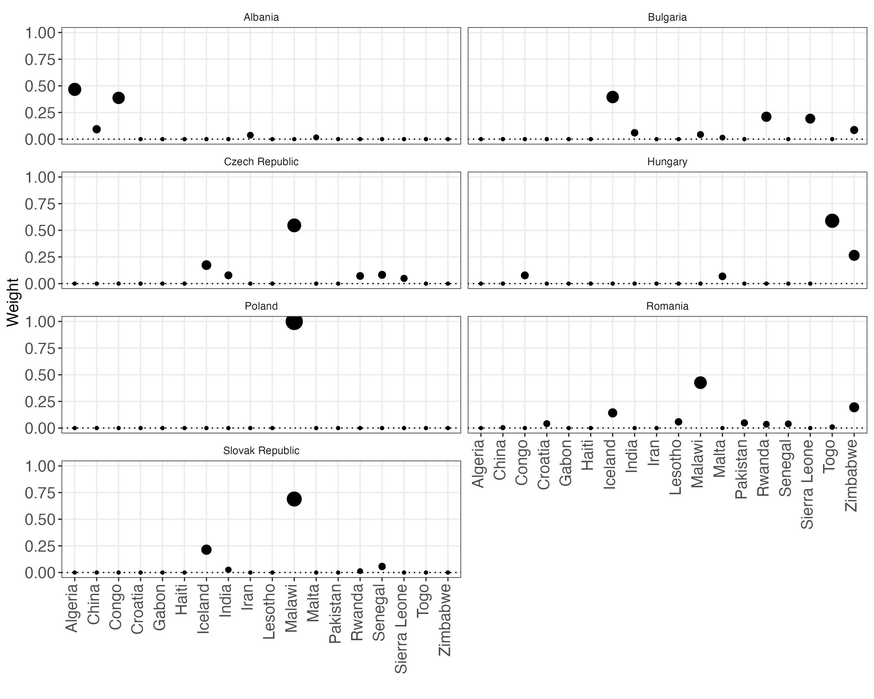
(c) $\widehat{w}_{i}$

Notes: Blue bars report 90% prediction intervals, whereas blue shaded areas report 90% simultaneous prediction intervals. In-sample uncertainty is quantified using 200 simulations, whereas out-of-sample uncertainty is quantified using sub-Gaussian bounds.

Average post-treatment effect for each liberalized country ($\tau_{i\cdot}$). The second causal predictand of our interest is the average post-treatment effect for each of the six European countries we study. Specifically, we target the average effect over the period following the liberalization up to the year 2000. Figure 6 shows that in all countries the liberalization episode depressed the real income per capita. However, if we consider individual and simultaneous prediction intervals that possess high simultaneous coverage across treated units, we can see that no treated unit shows a negative average post-treatment effect with high probability.

Figure 6: Average Post-Treatment Effects $\widehat{\tau}_{i\cdot}$.

(a) $Y_{it}(T_{i})$ and $\widehat{Y}_{it}(\infty)$

(b) $\widehat{\tau}_{i\cdot}$

(c) $\widehat{w}_{i}$

Notes: Blue bars report 90% prediction intervals, whereas red bars report 90% simultaneous prediction intervals (that simultaneously cover six treated units). In-sample uncertainty is quantified using 200 simulations, whereas out-of-sample uncertainty is quantified using sub-Gaussian bounds. The small number at the bottom-right corner of panel (a) represents the number of periods over which the post-treatment average is computed.

Average treatment effect on countries liberalized in 1991 ($\tau_{\cdot k,1991}$). In this third exercise, we analyze the average treatment effect on the treated at 1991, that is, on countries that liberalized in 1991: Bulgaria, Czech Republic, Slovak Republic, and Slovenia. To study this causal predictand, we are again match on real GDP per capita and percentage of complete secondary schooling. In the Supplemental Appendix Section S.7 we also report the results using a simplex-type constraint and the results using only GDP $(M=1)$. Even in this case, the trajectory for the synthetic real income lies above the realized one, suggesting a negative impact of the liberalization event. However, once again, quantifying uncertainty shows that, with high probability, we can conclude that the two series are not different from each other.

Figure 7: Average Treatment Effects on the Treated in 1991 $\tau_{\cdot k,1991}$.

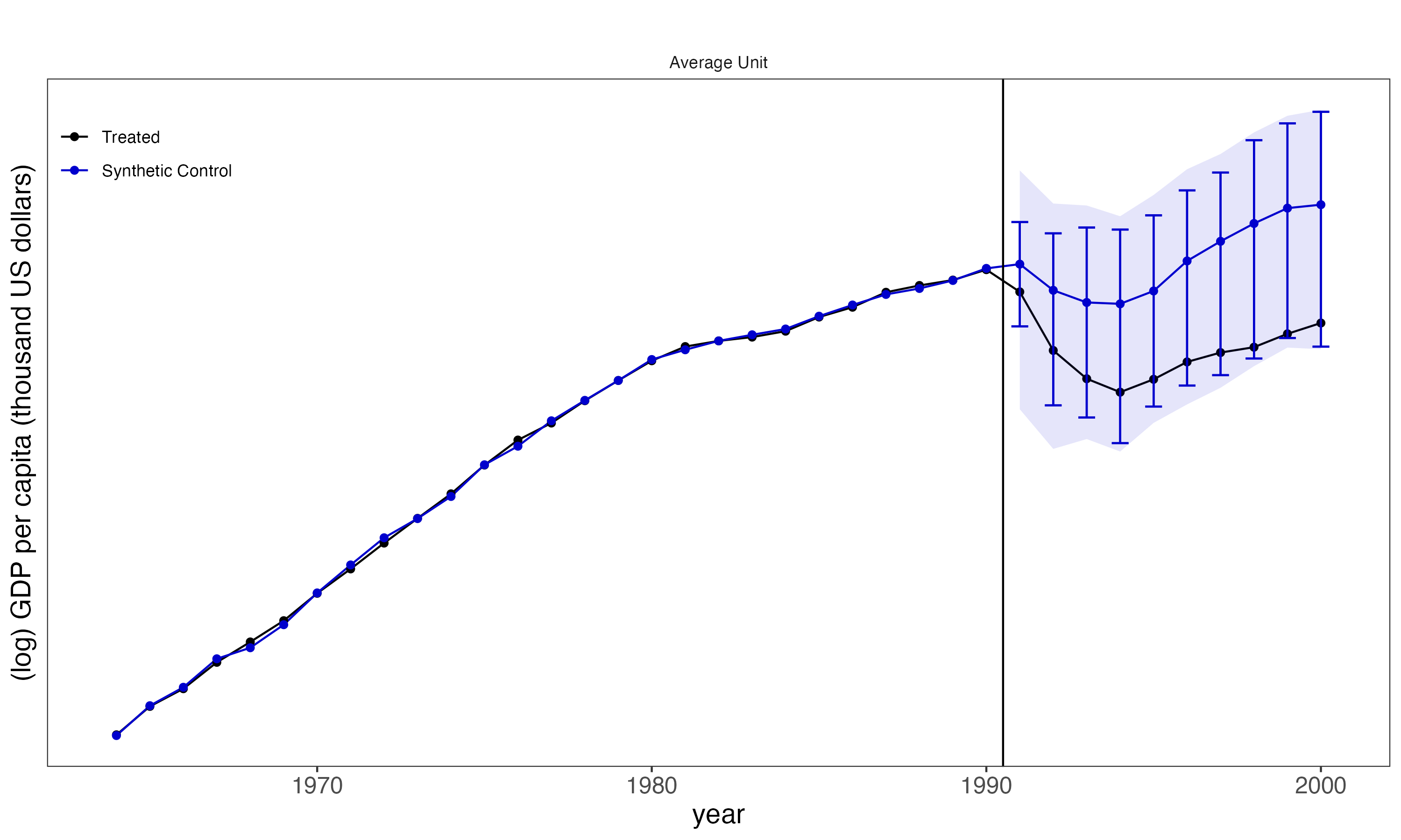
(a) $Y_{it}(T_{i})$ and $\widehat{Y}_{it}(\infty)$

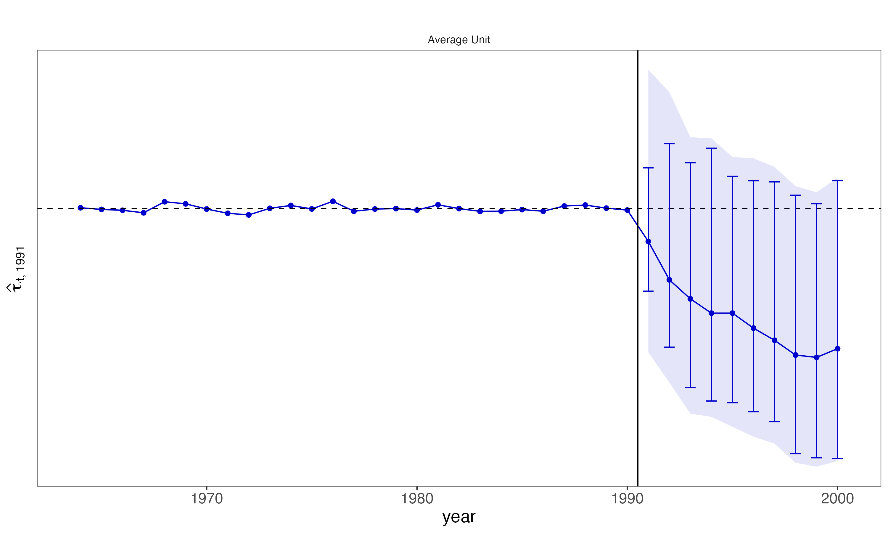
(b) $\widehat{\tau}_{\cdot k,1991}$

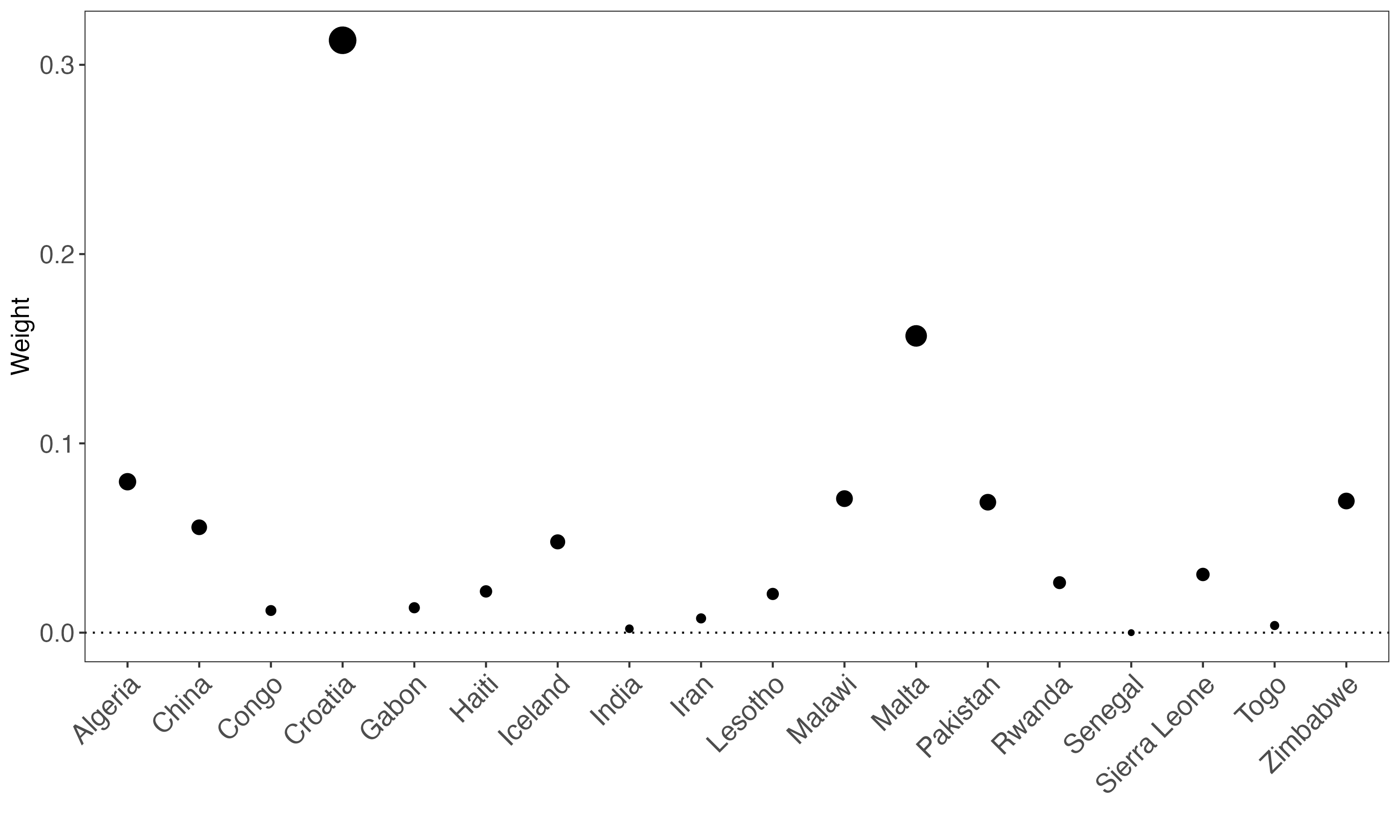
(c) $\widehat{w}_{i}$

Notes: Blue bars report 90% prediction intervals, whereas blue shaded areas report 90% simultaneous prediction intervals. In-sample uncertainty is quantified using 200 simulations, whereas out-of-sample uncertainty using sub-Gaussian bounds.

Average treatment effect on all liberalized countries ($\tau_{\cdot k}$). In this last and fourth exercise, we focus on a popular causal predictand: the average treatment effect on all the treated countries, that is, on all countries that liberalized, regardless of when they did so. We focus on the effects up to 10 periods after the adoption of liberalization, which occurs at different times for different countries. Figure 8 reports the results for liberalized countries in Europe. To compute this predictand, we first construct a synthetic control for each treated unit (see panel (c)) and then we pool such synthetic controls together in the post-treatment period to get a single prediction and a single prediction intervals. Panel (a) and panel (b) show that pooling across the 7 European countries that embarked on liberalization program helps reducing the uncertainty surrounding the synthetic trajectory. Indeed, this predictand is the only one that suggests that the trajectories for synthetic real income and actual real income differ with high probability for the average treated country.

Figure 8: Average Treatment Effects on the Treated $\tau_{\cdot k}$.

(a) $Y_{it}(T_{i})$ and $\widehat{Y}_{it}(\infty)$

(b) $\widehat{\tau}_{\cdot k}$

(c) $\widehat{w}_{i}$

Notes: Blue bars report 90% prediction intervals, whereas blue shaded areas report 90% simultaneous prediction intervals. In-sample uncertainty is quantified using 200 simulations, whereas out-of-sample uncertainty using sub-Gaussian bounds.

7 Conclusion

We developed prediction intervals to quantify the uncertainty of a large class of synthetic control predictions or estimators in settings with staggered treatment adoption. Because many synthetic control applications have a limited number of observations, our inference procedures are based on non-asymptotic concentration arguments. The construction of our prediction intervals is designed to capture two sources of uncertainty: the first is the construction or estimation of the synthetic control weights with pre-treatment data, and the second is the variability of the post-treatment outcomes. By combining both sources in a prediction interval, our procedure offers precise non-asymptotic coverage probability guarantees, and allows researchers to implement sensitivity analyses to assess how robust the conclusions of the analysis are to various levels of uncertainty. Our framework is general, allowing for one or multiple treated units, simultaneous or staggered treatment adoption, linear or non-linear constraints, and stationary or non-stationary data. To enhance implementation, we also showed how to recast the methods as conic optimization programs and how to choose the necessary tuning parameters in a principled data-driven way. We illustrated our methods with an empirical application studying the effect of economic liberalization on GDP for European countries in the 1990s, motivated by the work of Billmeier and Nannicini (2013).

All our methods are implemented in Python, R, and Stata software, which is publicly available and discussed in in detail in our companion article Cattaneo, Feng, Palomba and Titiunik (2023) and in Section S.4 of the Supplemental Appendix.

References

- Abadie (2021) Abadie, A. (2021), “Using Synthetic Controls: Feasibility, Data Requirements, and Methodological Aspects,” Journal of Economic Literature, 59, 391–425.
- Abadie et al. (2010) Abadie, A., Diamond, A., and Hainmueller, J. (2010), “Synthetic Control Methods for Comparative Case Studies: Estimating the Effect of California’s Tobacco Control Program,” Journal of the American Statistical Association, 105, 493–505.
- Abadie and Gardeazabal (2003) Abadie, A., and Gardeazabal, J. (2003), “The Economic Costs of Conflict: A Case Study of the Basque Country,” American Economic Review, 93, 113–132.
- Agarwal et al. (2021) Agarwal, A., Shah, D., Shen, D., and Song, D. (2021), “On Robustness of Principal Component Regression,” Journal of the American Statistical Association, 116, 1731–1745.
- Ben-Michael et al. (2022) Ben-Michael, E., Feller, A., and Rothstein, J. (2022), “Synthetic Controls with Staggered Adoption,” Journal of the Royal Statistical Society, Series B, 84, 351–381.
- Bhagwati and Srinivasan (2001) Bhagwati, J., and Srinivasan, T. N. (2001), “Outward-Orientation and Development: Are Revisionists Right?” in Trade, Development and Political Economy, Springer, pp. 3–26.
- Billmeier and Nannicini (2013) Billmeier, A., and Nannicini, T. (2013), “Assessing Economic Liberalization Episodes: A Synthetic Control Approach,” Review of Economics and Statistics, 95, 983–1001.
- Boyd and Vandenberghe (2004) Boyd, S., and Vandenberghe, L. (2004), Convex Optimization, Cambridge University Press.
- Cattaneo et al. (2023) Cattaneo, M. D., Feng, Y., Palomba, F., and Titiunik, R. (2023), “scpi: Uncertainty Quantification for Synthetic Control Methods,” arXiv:2202.05984.
- Cattaneo et al. (2021) Cattaneo, M. D., Feng, Y., and Titiunik, R. (2021), “Prediction Intervals for Synthetic Control Methods,” Journal of the American Statistical Association, 116, 1865–1880.
- Chernozhukov et al. (2021a) Chernozhukov, V., Wüthrich, K., and Zhu, Y. (2021a), “Distributional Conformal Prediction,” Proceedings of the National Academy of Sciences, 118, e2107794118.
- Chernozhukov et al. (2021b) Chernozhukov, V., Wüthrich, K., and Zhu, Y. (2021b), “An Exact and Robust Conformal Inference Method for Counterfactual and Synthetic Controls,” Journal of the American Statistical Association, 116, 1849–1864.
- DeJong and Ripoll (2006) DeJong, D. N., and Ripoll, M. (2006), “Tariffs and Growth: An Empirical Exploration of Contingent Relationships,” The Review of Economics and Statistics, 88, 625–640.
- Giavazzi and Tabellini (2005) Giavazzi, F., and Tabellini, G. (2005), “Economic and Political Liberalizations,” Journal of Monetary Economics, 52, 1297–1330.
- Levine and Renelt (1992) Levine, R., and Renelt, D. (1992), “A Sensitivity Analysis of Cross-Country Growth Regressions,” American Economic Review, 82, 942–963.
- Li (2020) Li, K. T. (2020), “Statistical Inference for Average Treatment Effects Estimated by Synthetic Control Methods,” Journal of the American Statistical Association, 115, 2068–2083.
- Masini and Medeiros (2021) Masini, R., and Medeiros, M. C. (2021), “Counterfactual Analysis with Artificial Controls: Inference, High Dimensions and Nonstationarity,” Journal of the American Statistical Association, 116, 1773–1788.
- Sachs et al. (1995) Sachs, J. D., Warner, A., Åslund, A., and Fischer, S. (1995), “Economic Reform and the Process of Global Integration,” Brookings Papers on Economic Activity, 1995, 1–118.
- Shaikh and Toulis (2021) Shaikh, A. M., and Toulis, P. (2021), “Randomization Tests in Observational Studies with Staggered Adoption of Treatment,” Journal of the American Statistical Association, 116, 1835–1848.
- Shen et al. (2022) Shen, D., Ding, P., Sekhon, J., and Yu, B. (2022), “A Tale of Two Panel Data Regressions,” arXiv:2207.14481.
- Shi et al. (2023) Shi, X., Miao, W., Hu, M., and Tchetgen, E. T. (2023), “Theory for Identification and Inference with Synthetic Controls: A Proximal Causal Inference Framework,” arXiv:2108.13935.
- Vovk (2012) Vovk, V. (2012), “Conditional Validity of Inductive Conformal Predictors,” in JMLR: Workshop and Conference Proceedings 25, Asian Conference on Machine Learning, pp. 475–490.
- Wacziarg and Welch (2008) Wacziarg, R., and Welch, K. H. (2008), “Trade Liberalization and Growth: New Evidence,” The World Bank Economic Review, 22, 187–231.
- Wainwright (2019) Wainwright, M. J. (2019), High-Dimensional Statistics: A Non-Asymptotic Viewpoint, Cambridge University Press.