Parameterized Approaches to Orthogonal Compaction

Abstract

Orthogonal graph drawings are used in applications such as UML diagrams, VLSI layout, cable plans, and metro maps. We focus on drawing planar graphs and assume that we are given an orthogonal representation that describes the desired shape, but not the exact coordinates of a drawing. Our aim is to compute an orthogonal drawing on the grid that has minimum area among all grid drawings that adhere to the given orthogonal representation.

This problem is called orthogonal compaction (OC) and is known to be NP-hard, even for orthogonal representations of cycles [Evans et al. 2022]. We investigate the complexity of OC with respect to several parameters. Among others, we show that OC is fixed-parameter tractable with respect to the most natural of these parameters, namely, the number of kitty corners of the orthogonal representation: the presence of pairs of kitty corners in an orthogonal representation makes the OC problem hard. Informally speaking, a pair of kitty corners is a pair of reflex corners of a face that point at each other. Accordingly, the number of kitty corners is the number of corners that are involved in some pair of kitty corners.

1 Introduction

In a planar orthogonal drawing of a planar graph $G$ each vertex is mapped to a distinct point of the plane and each edge is represented as a sequence of horizontal and vertical segments. A planar graph $G$ admits a planar orthogonal drawing if and only if it has vertex-degree at most four. A planar orthogonal representation $H$ of $G$ is an equivalence class of planar orthogonal drawings of $G$ that have the same “shape”, i.e., the same planar embedding, the same ordered sequence of bends along the edges, and the same vertex angles. A planar orthogonal drawing belonging to the equivalence class $H$ is simply called a drawing of $H$. For example, Figs. 1(a) and 1(b) are drawings of the same orthogonal representation, while Fig. 1(c) is a drawing of the same graph with a different shape.

Given a planar orthogonal representation $H$ of a connected planar graph $G$, the orthogonal compaction problem (OC for short) for $H$ asks to compute a minimum-area drawing of $H$. More formally, it asks to assign integer coordinates to the vertices and to the bends of $H$ such that the area of the resulting planar orthogonal drawing is minimum over all drawings of $H$. The area of a drawing is the area of the minimum bounding box that contains the drawing. For example, the drawing in Fig. 1(a) has area $7\times 5=35$, whereas the drawing in Fig. 1(b) has area $7\times 4=28$, which is the minimum for that orthogonal representation.

The area of a graph layout is considered one of the most relevant readability metrics in orthogonal graph drawing (see, e.g., [16, 26]). Compact grid drawings are desirable as they yield a good overview without neglecting details. For this reason, the OC problem is widely investigated in the literature. Bridgeman et al. [11] showed that OC can be solved in linear time for a subclass of planar orthogonal representations called turn-regular. Informally speaking, a face of a planar orthogonal representation $H$ is turn-regular if it does not contain any pair of so-called kitty corners, i.e., a pair of reflex corners (turns of $270^{\circ}$) that point to each other; a representation is turn-regular if all its faces are turn-regular. See Fig. 1 and refer to Section 2 for a formal definition. On the other hand, Patrignani [30] proved that, unfortunately, OC is NP-hard in general. Evans et al. [22] showed that OC remains NP-hard even for orthogonal representations of simple cycles. Since cycles have constant pathwidth (namely 2), this immediately shows that we cannot expect an FPT (or even an XP) algorithm parameterized by pathwidth alone unless P = NP. The same holds for parametrizations with respect to treewidth since the treewidth of a graph is upper bounded by its pathwidth.

In related work, Bannister et al. [3] showed that several problems of compacting not necessarily planar orthogonal graph drawings to use the minimum number of rows, area, length of longest edge, or total edge length cannot be approximated better than within a polynomial factor of optimal (if P$\neq$NP). They also provided an FPT algorithm for testing whether a drawing can be compacted to a small number of rows. Note that their algorithm does not solve the planar case because the algorithm is allowed to change the embedding.

(a) area = 35

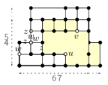
(b) area = 28

(c) area = 24

Figure 1: (a) Drawing of a non-turn-regular orthogonal representation $H$; vertices $u$ and $v$ point to each other in the filled internal face, thus they represent a pair of kitty corners. Vertices $w$ and $z$ are a pair of kitty corners in the external face. (b) Another drawing of $H$ with minimum area. (c) Minimum-area drawing of a turn-regular orthogonal representation of the same graph.

The research in this paper is motivated by the relevance of the OC problem and by the growing interest in parameterized approaches for NP-hard problems in graph drawing [24]. Recent works on the subject include parameterized algorithms for book embeddings and queue layouts [2, 7, 8, 10, 27], upward planar drawings [10, 12], orthogonal planarity testing and grid recognition [18, 25], clustered planarity and hybrid planarity [15, 28, 29], 1-planar drawings [1], and crossing minimization [4, 20, 21].

Contribution.

Extending this line of research, we initiate the study of the parameterized complexity of OC and investigate several parameters:

• Number of kitty corners. Given that OC can be solved efficiently for orthogonal representations without kitty corners, the number of kitty corners (that is, the number of corners involved in some pair of kitty corners) is a very natural parameter for OC. We show that OC is fixed-parameter tractable (FPT) with respect to the number of kitty corners (Theorem 3.1 in Section 3).

• Number of faces. Since OC remains NP-hard for orthogonal representations of simple cycles [22], OC is para-NP-hard when parameterized by the number of faces. Hence, we cannot expect an FPT (or even an XP) algorithm in this parameter alone, unless P$\,=\,$NP. However, for orthogonal representations of simple cycles we show the existence of a polynomial kernel for OC when parameterized by the number of kitty corners (Theorem 4.1 in Section 4).

• Maximum face-degree. The maximum face-degree is the maximum number of vertices on the boundary of a face. Since both the NP-hardness reductions by Patrignani [30] and Evans et al. [22] require faces of linear size, it is interesting to know whether faces of constant size make the problem tractable. We prove that this is not the case, i.e., OC remains NP-hard when parameterized by the maximum face degree (Theorem 5.1 in Section 5).

• Height. The height of an orthogonal representation is the minimum number of distinct y-coordinates required to draw the representation. Since a $w\times h$ grid has pathwidth at most $h$, graphs with bounded height have bounded pathwidth, but the converse is generally not true [9]. In fact, we show that OC admits an XP algorithm parameterized by the height of the given representation (see Theorem 6.1 in Section 6). In this context, we remark that a related problem has been considered by Chaplick et al. [13]. Given a planar graph $G$, they defined $\bar{\pi}^{1}_{2}(G)$ to be the minimum number of distinct y-coordinates required to draw the graph straight-line. (In their version of the problem, however, the embedding of $G$ is not fixed.)

We start with some basics in Section 2 and close with open problems in Section 7. Theorems marked with a (clickable) $\star$ are proven in detail in the appendix.

2 Basic Definitions

Let $G=(V,E)$ be a connected planar graph of vertex-degree at most four and let $\Gamma$ be a planar orthogonal drawing of $G$. We assume that in $\Gamma$ all the vertices and bends have integer coordinates, i.e., we assume that $\Gamma$ is an integer-coordinate grid drawing. Two planar orthogonal drawings $\Gamma_{1}$ and $\Gamma_{2}$ of $G$ are shape-equivalent if: $(i)$ $\Gamma_{1}$ and $\Gamma_{2}$ have the same planar embedding; $(ii)$ for each vertex $v\in V$, the geometric angles at $v$ (formed by any two consecutive edges incident on $v$) are the same in $\Gamma_{1}$ and $\Gamma_{2}$; $(iii)$ for each edge $e=(u,v)\in E$ the sequence of left and right bends along $e$ while moving from $u$ to $v$ is the same in $\Gamma_{1}$ and $\Gamma_{2}$. An orthogonal representation $H$ of $G$ is a class of shape-equivalent planar orthogonal drawings of $G$. It follows that an orthogonal representation $H$ is completely described by a planar embedding of $G$, by the values of the angles around each vertex (each angle being a value in the set $\{90^{\circ},180^{\circ},270^{\circ},360^{\circ}\}$), and by the ordered sequence of left and right bends along each edge $(u,v)$, moving from $u$ to $v$; if we move from $v$ to $u$, then this sequence and the direction (left/right) of each bend are reversed. If $\Gamma$ is a planar orthogonal drawing in the class $H$, then we also say that $\Gamma$ is a drawing of $H$. Without loss of generality, we also assume that an orthogonal representation $H$ comes with a given “orientation”, i.e., for each edge segment $\overline{pq}$ of $H$ (where $p$ and $q$ correspond to vertices or bends), we fix whether $p$ lies to the left, to the right, above, or below $q$.

Turn-regular orthogonal representations.

Let $H$ be a planar orthogonal representation. For the purpose of the OC problem, and without loss of generality, we always assume that each bend in $H$ is replaced by a degree-2 vertex. Let $f$ be a face of a planar orthogonal representation $H$ and assume that the boundary of $f$ is traversed counterclockwise (resp. clockwise) if $f$ is internal (resp. external). Let $u$ and $v$ be two reflex vertices of $f$. Let $\textrm{rot}(u,v)$ be the number of convex corners minus the number of reflex corners encountered while traversing the boundary of $f$ from $u$ (included) to $v$ (excluded); a reflex vertex of degree one is counted like two reflex vertices. We say that $u$ and $v$ is a pair of kitty corners of $f$ if $\textrm{rot}(u,v)=2$ or $\textrm{rot}(v,u)=2$. A vertex is a kitty corner if it is part of a pair of kitty corners. A face $f$ of $H$ is turn-regular if it does not contain a pair of kitty corners. The representation $H$ is turn-regular if all faces are turn-regular.

For information on parameterized complexity, we refer to books such as [14, 19, 23] and Appendix 0.A.

3 Number of Kitty Corners: An FPT Algorithm

Turn-regular orthogonal representation can be compacted optimally in linear time [11]. We recall this result and then describe our FPT algorithm.

Upward planar embeddings and saturators.

Let $D=(V,E)$ be a plane DAG, i.e., an acyclic digraph with a given planar embedding. An upward planar drawing $\Gamma$ of $D$ is an embedding-preserving drawing of $D$ where each vertex $v$ is mapped to a distinct point of the plane and each edge is drawn as a simple Jordan arc monotonically increasing in the upward direction. Such a drawing exists if and only if $D$ is the spanning subgraph of a plane $st$-graph, i.e., a plane digraph with a unique source $s$ and a unique sink $t$, which are both on the external face [17]. Let $S$ be the set of sources of $D$, $T$ be the set of sinks, and $I=V\setminus(S\cup T)$. $D$ is bimodal if, for every vertex $v\in I$, the outgoing edges (and hence the incoming edges) of $v$ are consecutive in the clockwise order around $v$. If an upward planar drawing $\Gamma$ of $D$ exists, then $D$ is necessarily bimodal and $\Gamma$ uniquely defines the left-to-right orderings of the outgoing and incoming edges of each vertex. This set of orderings (for all vertices of $D$) is an upward planar embedding of $D$, and is regarded an equivalence class of upward planar drawings of $D$. A plane DAG with a given upward planar embedding is an upward plane DAG.

(a)

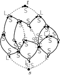
(b)

Figure 2: (a) An upward plane DAG $D$ and the corresponding upward labeling. (b) A plane $st$-graph obtained by augmenting $D$ with a complete saturator (dotted edges).

Let $e_{1}$ and $e_{2}$ be two consecutive edges on the boundary of a face $f$ of a bimodal plane digraph $D$, and let $v$ be their common vertex. Vertex $v$ is a source switch of $f$ (resp. a sink switch of $f$) if both $e_{1}$ and $e_{2}$ are outgoing edges (resp. incoming edges) of $v$. Note that, for each face $f$, the number $n_{f}$ of source switches of $f$ equals the number of sink switches of $f$. The capacity of $f$ is the function $\mathsf{cap}(f)=n_{f}-1$ if $f$ is an internal face and $\mathsf{cap}(f)=n_{f}+1$ if $f$ is the external face. If $\Gamma$ is an upward planar drawing of $D$, then each vertex $v\in S\cup T$ has exactly one angle larger than $180^{\circ}$, called a large angle, in one of its incident faces, and $\deg(v)-1$ angles smaller than $180^{\circ}$, called small angles, in its other incident faces. For a source or sink switch of $f$, assign either a label $\mathsf{L}$ or a label $\mathsf{S}$ to its angle in $f$, depending on whether this angle is large or small. For each face $f$ of $D$, the number of $\mathsf{L}$-labels determined by $\Gamma$ equals $\mathsf{cap}(f)$ [6]. Conversely, given an assignment of $\mathsf{L}$- and $\mathsf{S}$-labels to the angles at the source and sink switches of $D$; for each vertex $v$, $\mathsf{L}(v)$ (resp. $\mathsf{S}(v)$) denotes the number of $\mathsf{L}$- (resp. of $\mathsf{S}$-) labels at the angles of $v$. For each face $f$, $\mathsf{L}(f)$ (resp. $\mathsf{S}(f)$) denotes the number of $\mathsf{L}$- (resp. of $\mathsf{S}$-) labels at the angles in $f$. Such an assignment corresponds to the labels induced by an upward planar drawing of $D$ if and only if the following properties hold [6]: (a) $\mathsf{L}(v)=0$ for each $v\in I$ and $\mathsf{L}(v)=1$ for each $v\in S\cup T$; (b) $\mathsf{L}(f)=\mathsf{cap}(f)$ for each face $f\in F$. We call such an assignment an upward labeling of $D$, as it uniquely corresponds to (and hence describes) an upward planar embedding of $D$; see Fig. 2(a). We will implicitly assume that a given upward plane DAG is described by an upward labeling.

Given an upward plane DAG $D$, a complete saturator of $D$ is a set of vertices and edges, not belonging to $D$, used to augment $D$ to a plane $st$-graph $D^{\prime}$. More precisely, a complete saturator consists of a source $s$ and a sink $t$, which will belong to the external face of $D^{\prime}$, and of a set of edges where each edge $(u,v)$ is called a saturating edge and fulfills one of the following conditions (see, e.g., Fig. 2(b)): (i) $u,v\notin\{s,t\}$ and $u,v$ are both source switches of the same face $f$ such that $u$ has label $\mathsf{S}$ in $f$ and $v$ has label $\mathsf{L}$ in $f$; in this case $u$ saturates $v$. (ii) $u,v\notin\{s,t\}$ and $u,v$ are both sink switches of the same face $f$ such that $u$ has label $\mathsf{L}$ in $f$ and $v$ has label $\mathsf{S}$ in $f$; in this case $v$ saturates $u$. (iii) $u=s$ and $v$ is a source switch of the external face with an $\mathsf{L}$ angle. (iv) $v=t$ and $u$ is a sink switch of the external face with an $\mathsf{L}$ angle.

We now recall how to compact in linear time a turn-regular orthogonal representation. Let $H$ be an orthogonal representation that is not necessarily turn-regular. Let $D_{x}$ be the plane DAG whose vertices correspond to the maximal vertical chains of $H$ and such that two vertices of $D_{x}$ are connected by an edge oriented rightward, if the corresponding vertical chains are connected by a horizontal segment in $H$. Define the upward plane DAG $D_{y}$ symmetrically, where the vertices correspond to the maximal horizontal chains of $H$ and where the edges are oriented upward. Refer to Fig. 3. $D_{x}$ and $D_{y}$ are both upward plane DAGs (for $D_{x}$ rotate it by $90^{\circ}$ to see all edges flowing in the upward direction). For a vertex $v$ of $H$, $c_{x}(v)$ (resp. $c_{y}(v)$) denotes the vertex of $D_{x}$ (resp. of $D_{y}$) corresponding to the maximal vertical (resp. horizontal) chain of $H$ that contains $v$. For any two vertices $u$ and $v$ of $H$ such that $c_{x}(u)\neq c_{x}(v)$, we write $u\rightsquigarrow_{x}v$ if there exists a directed path from $c_{x}(u)$ to $c_{x}(v)$ in $D_{x}$. We also write $u\leftrightsquigarrow_{x}v$ if either $u\rightsquigarrow_{x}v$ or $v\rightsquigarrow_{x}u$, while $u\not\leftrightsquigarrow_{x}v$ means that neither $u\rightsquigarrow_{x}v$ nor $v\rightsquigarrow_{x}u$. The notations $u\rightsquigarrow_{y}v$, $v\rightsquigarrow_{y}u$, $u\leftrightsquigarrow_{y}v$, and $u\not\leftrightsquigarrow_{y}v$ are used symmetrically referring to $D_{y}$ when $c_{y}(u)\neq c_{y}(v)$.

Bridgeman et al. [11] showed that $H$ is turn-regular if and only if, for every two vertices $u$ and $v$ in $H$, we have $u\leftrightsquigarrow_{x}v$, or $u\leftrightsquigarrow_{y}v$, or both. This is equivalent to saying that the relative position along the $x$-axis or the relative position along the $y$-axis (or both) between $u$ and $v$ is fixed over all drawings of $H$. Under this condition, the OC problem for $H$ can be solved by independently solving in $O(n)$ time a pair of 1D compaction problems for $H$, one in the $x$-direction and the other in the $y$-direction. The 1D compaction in the $x$-direction consists of: $(i)$ augmenting $D_{x}$ to become a plane $st$-graph by means of a complete saturator; $(ii)$ computing an optimal topological numbering $X$ of $D_{x}$ (see [16], p. 89); each vertex $v$ of $H$ receives an x-coordinate $x(v)$ such that $x(v)=X(c_{x}(v))$. We recall that a topological numbering of a DAG $D$ is an assignment of integer numbers to the vertices of $D$ such that if there is a path from $u$ to $v$ then $u$ is assigned a number smaller than the number of $v$. A topological numbering is optimal if the range of numbers that is used is the minimum possible. Regarding step $(i)$ of the 1D compaction, note that $D_{x}$ admits a unique complete saturator when $H$ is turn-regular [11]. This is due to the absence of kitty corners in each face of $H$. The 1D compaction in the $y$-direction is solved symmetrically, so that each vertex $v$ receives a y-coordinate $y(v)=Y(c_{y}(v))$. Figure 3 illustrates this process.

(a)

(b)

(c)

(d)

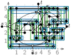
(e)

(f)

Figure 3: (a) A turn-regular orthogonal representation $H$. (b)–(c) The maximal horizontal and vertical chains of $H$ are highlighted. (d) The upward plane DAG $D_{x}$ with its complete saturator (dashed edges) and an optimal topological numbering. (e) The same for $D_{y}$. (f) A minimum-area drawing of $H$ where the x- and y-coordinates correspond to the two optimal topological numberings.

Unfortunately, if $H$ is not turn-regular, the aforementioned approach fails. This is because there are in general many potential complete saturators for augmenting the two upward plane DAGs $D_{x}$ and $D_{y}$ to plane $st$-graphs. Also, even when an $st$-graph for each DAG is obtained from a complete saturator, computing independently an optimal topological numbering for each of the two $st$-graphs may lead to non-planar drawings if no additional relationships are established for the coordinates of kitty corner pairs, because for a pair $\{u,v\}$ of kitty corners we have $u\not\leftrightsquigarrow_{x}v$ and $u\not\leftrightsquigarrow_{y}v$. We now prove that OC is fixed-parameter-tractable when parameterized by the number of kitty corners.

Theorem 3.1

Let $H$ be a planar orthogonal representation with $n$ vertices and $k>0$ kitty corners. There exists an $O(2^{11k}n\log n)$-time algorithm that computes a minimum-area drawing of $H$.

Proof

Let $H$ be an orthogonal representation and let $k$ be the number of kitty corners of $H$. For each pair $\{u,v\}$ of kitty corners, we guess the relative positions of $u$ and $v$ in a drawing of $H$, i.e., $x(u)\lesseqgtr x(v)$ and $y(u)\lesseqgtr y(v)$.

Namely, we generate all maximal plane DAGs (together with an upward planar embedding) that can be incrementally obtained from $D_{x}$ by repeatedly applying the following sequence of steps: Guess a pair $\{u,v\}$ of kitty corners of $H$ such that $c_{x}(u)$ and $c_{x}(v)$ belong to the same face; for such a pair either add a directed edge $(c_{x}(u),c_{x}(v))$ (which establishes that $x(u)<x(v)$), or add a directed edge $(c_{x}(v),c_{x}(u))$ (which establishes that $x(u)>x(v)$), or identify $c_{x}(u)$ and $c_{x}(v)$ (which establishes that $x(u)=x(v)$); this last operation corresponds to adding in $H$ a vertical segment between $u$ and $v$, thus merging the vertical chain of $u$ with the vertical chain of $v$. Analogously, we generate from $D_{y}$ a set of maximal plane DAGs (together with an upward planar embedding). Let $\overline{D_{x}}$ and $\overline{D_{y}}$ be two upward plane DAGs generated as above. We augment $\overline{D_{x}}$ (resp. $\overline{D_{y}}$) with a complete saturator that makes it a plane $st$-graph. Observe that, by construction, neither $\overline{D_{x}}$ nor $\overline{D_{y}}$ contain two non-adjacent vertices in the same face whose corresponding chains of $H$ have a pair of kitty corners. Hence their complete saturators are uniquely defined. We finally compute a pair of optimal topological numberings to determine the $x$- and the y-coordinates of each vertex of $H$ as in [11]. Note that, for some pairs of $\overline{D_{x}}$ and $\overline{D_{y}}$, the procedure described above may assign $x$- and y-coordinates to the vertices of $H$ that do not lead to a planar orthogonal drawing. If so, we discard the solution. Conversely, for those solutions that correspond to (planar) drawings of $H$, we compute the area and, at the end, we keep one of the drawings having minimum area.

(a)

(b)

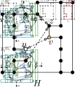
(c)

(d)

Figure 4: (a) An orthogonal representation $H$ with three pairs of kitty corners, $\{u,v\}$, $\{w,z\}$, and $\{q,z\}$. (b) Two distinct (saturated) upward plane DAGs $\overline{D_{x}}$ and $\overline{D_{x}}^{\prime}$, and their optimal topological numberings $X$ and $X^{\prime}$; in $\overline{D_{x}}^{\prime}$ the nodes $c_{x}(u)$ and $c_{x}(v)$ are identified (filled square). (c) Two distinct (saturated) upward plane DAGs $\overline{D_{y}}$ and $\overline{D_{y}}^{\prime}$ and their optimal topological numberings $Y$ and $Y^{\prime}$. (d) Drawings derived from the four different combinations of the topological numberings: $\Gamma_{1}$ and $\Gamma_{3}$ have sub-optimal areas, $\Gamma_{2}$ has minimum area, and $\Gamma_{4}$ is non-planar (the bold red face is self-crossing).

Figure 4 shows a non-turn-regular orthogonal representation; Fig. 4(d) depicts four drawings resulting from different pairs of upward plane DAGs, each establishing different $x$- and $y$-relationships between pairs of kitty corners. One of the drawings has minimum area; another one is not planar and therefore discarded.

We now analyze the runtime. Let $\{f_{1},f_{2},\dots,f_{h}\}$ be the set of faces of $H$, and let $k_{i}$ be the number of kitty corners in $f_{i}$. Denote by $a_{i}$ the number of distinct maximal planar augmentations of $f_{i}$ with edges that connect pairs of kitty corners. An upper bound to the value of $a_{i}$ is the number $c_{k_{i}}$ of distinct maximal outerplanar graphs with $k_{i}$ vertices, which corresponds to the number of distinct triangulations of a convex polygon with $k_{i}$ vertices. It is known that $c_{k_{i}}$ equals the $(k_{i}-2)$-nd Catalan number (see, e.g., [31]), whose standard estimate is $c_{k_{i}-2}\sim\frac{4^{k_{i}-2}}{(k_{i}-2)^{3/2}\sqrt{\pi}}$. Therefore, $a_{i}\in O(4^{k_{i}})$. Note that all distinct triangulations of a convex polygon can easily be generated with a recursive approach.

Now, for each edge $(u,v)$ of a maximal planar augmentation of $f_{i}$ such that $\{u,v\}$ is a pair of kitty corners in $H$, we have to consider three alternative possibilities: $\overline{D_{x}}$ has a directed edge $(c_{x}(u),c_{x}(v))$, or $\overline{D_{x}}$ has a directed edge $(c_{x}(v),c_{x}(u))$, or $c_{x}(u)$ and $c_{x}(v)$ are identified in $\overline{D_{x}}$. The same happens for $\overline{D_{y}}$. Therefore, since the number of edges of a maximal outerplanar graph on $k_{i}$ vertices is $2k_{i}-3$, the number of different configurations to be considered for each face $f_{i}$ both in $\overline{D_{x}}$ and in $\overline{D_{y}}$ is $O(3^{2k_{i}}4^{k_{i}})\cdot O(3^{2k_{i}}4^{k_{i}})=O(36^{2k_{i}})=O(2^{11k_{i}})$. By combining these possible configurations over all faces of $H$, we obtain $O(2^{11k})$ pairs of possible configurations for $\overline{D_{x}}$ and in $\overline{D_{y}}$ (clearly, $\sum_{i=0}^{h}k_{i}=k$). For each such pair, we augment each of the two upward plane DAGs to a plane $st$-graph and compute an optimal topological numbering in $O(n)$ time. Then we test whether the drawing resulting from the two topological numberings is planar, which can be done in $O(n\log n)$ time by a sweep line algorithm (see, e.g., [5, 32]). It follows that the whole testing algorithm takes $O(2^{11k}n\log n)$ time.

4 A Polynomial Kernel for Cycle Graphs

In this section, we prove the following theorem.

Theorem 4.1

Parameterized by the number of kitty corners, OC admits a compression with linear number of vertices (and a polynomial kernel) on cycle graphs.

Let $G$ be a cycle graph with an orthogonal representation $H$. We traverse the (single) internal face of $H$ in counterclockwise direction to define a labeled digraph $G^{\rightarrow}$: label each edge $\mathsf{E}$, $\mathsf{W}$, $\mathsf{N}$, or $\mathsf{S}$ based on its direction, and label each vertex $\mathsf{F}$, $\mathsf{C}$ and $\mathsf{R}$ based on whether it is flat, convex or reflex from the internal face. Given two vertices $u$ and $v$, let $P_{u,v}$ be the directed path from $u$ to $v$ in $G^{\rightarrow}$. For an edge $e$, let $\mathsf{weight}(e)$ be the weight of $e$. (The addition of edge weights will yield a compression, which can be turned into a kernel.)

Let $\langle c_{1},\ldots,c_{k},c_{k+1}=c_{1}\rangle$ be the cyclic order of kitty corners of $H$ in $G^{\rightarrow}$. For each $P_{c_{i},c_{i+1}}$, we bound the number of internal vertices. As $G^{\rightarrow}$ is the union of these paths, this bounds the size of the reduced instance. We now present reduction rules to reduce the number of vertices on these paths. We always apply them in the given order. We first reduce a path of $\mathsf{F}$-vertices to a weighted edge:

Reduction Rule 1. We reduce every path $P_{u,v}$, whose internal vertices are all labeled $\mathsf{F}$, to a directed edge $(u,v)$ with $\mathsf{weight}((u,v))=\sum_{e\in E(P_{u,v})}\mathsf{weight}(e)$.

Thus, next assume that $G^{\rightarrow}$ does not have any $\mathsf{F}$-vertex. Observe that if $P_{c_{i},c_{i+1}}$ has at least $7$ internal vertices, then either all the internal vertices are labeled $\mathsf{R}$ or $P_{c_{i},c_{i+1}}$ has an internal subpath with a labeling from $\{\mathsf{RCR},\mathsf{RCCC},\mathsf{RCCR},\mathsf{RRRC},$ $\mathsf{CRC},\mathsf{CRRC},\mathsf{CRRR},\mathsf{CCCR}\}$. So, in the former case, we give a counting rule to count all the $\mathsf{R}$ vertices against the kitty corners. Moreover, in the later case, we give reduction rules to reduce those paths. This, in turn, will bound the size of the reduced instance. Due to lack of space, we refer the readers to Appendix 0.B for the details.

5 Maximum Face Degree: Parameterized Hardness

We show that the problem remains NP-hard even if all faces have constant degree. Our proof elaborates on ideas of Patrignani’s NP-hardness proof for OC [30].

Theorem 5.1 (th:hard-face-degree*)

$\star$] OC is para-NP-hard when parameterized by the maximum face degree.

Proof (sketch)

Patrignani [30] reduces from SAT to OC. For a SAT instance $\phi$ with $n$ variables and $m$ clauses, he creates an orthogonal representation $H_{\phi}$ that admits an orthogonal grid drawing of size $w_{\phi}\cdot h_{\phi}$ if and only if $\phi$ is satisfiable.

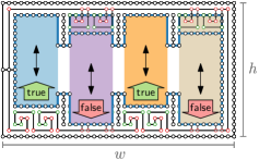
Figure 5: The shifting variable rectangles (shaded) and the belt (the path with hexagonal vertices) in the NP-hardness proof by Patrignani [30].

Every variable is represented by a variable rectangle inside a frame; see Fig. 5. Between the frame and the rectangles, there is a belt: a long path of 4 reflex vertices alternating with 4 convex vertices that ensures that every variable rectangle is either shifted to the top ($\mathsf{true}$) or to the bottom ($\mathsf{false}$).

Figure 6: A clause gadget in the NP-hardness proof by Patrignani [30] for the clause $\overline{X_{1}}\vee X_{2}\vee\overline{X_{4}}$: the variable-clause rectangles (color shaded), the blocking rectangles (gray shaded), and the pathway (the path with diamond vertices). The segment that corresponds to a fulfilled variable assignment for this clause $(X_{2})$ is highlighted.

Every clause is represented by a chamber through the variable rectangles with one or two blocker rectangles depending on the occurrence of the variable in the clause; see Fig. 6. Into the chamber, a pathway is inserted that can only be drawn if there is a gap between blocker rectangles is vertically aligned with a gap between two variable-clause rectangles, which represents a fulfilled literal.

We now briefly sketch how to adjust the reduction.

Figure 7: The clause gadget of Fig. 6 adjusted to constant face degree.

For the clause gadgets, there are two large faces of size $O(m)$; above and below the pathway. To avoid these, we connect the pathway to the top and the bottom boundary of each of the variable-clause rectangles as in see Fig. 7.

(a)

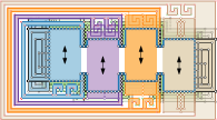
(b)

Figure 8: The frame in our adjusted NP-hardness reduction. (a) The left and right extensions of the variable rectangles; (b) the belts around the variable rectangles.

For the face around the variable rectangles, we refine the left and the right side (that both have $O(m)$ vertices) by adding $O(m)$ rectangles of constant degree in a tree-like shape; see Fig. 8(a). Instead of a single long belt, we use a small belt of constant length around every variable rectangle that lies inside its own frame and extend the variable rectangles vertically; see Fig. 8(b).

After these adjustments, all faces have constant degree as desired.

6 Height of the Representation: An XP Algorithm

By “guessing” for every column of the drawing what lies on each grid point, we obtain an XP algorithm for OC parameterized by the height of the representation.

Theorem 6.1 (th:xp-height*)

$\star$] OC is XP when parameterized by the height of a given orthogonal representation of a connected planar graph of maximum degree 4.

Proof (sketch)

Let $H$ be the given orthogonal representation, let $n$ be the number of vertices of $H$, let $b$ the number of bends in $H$, and let $h\geq 1$. We want to decide, in $(O(n+b))^{O(h)}$ time, whether $H$ admits an orthogonal drawing on a grid with $h$ horizontal lines. Given a solution, that is, a drawing of $H$, we can remove any grid column that does not contain any vertex or bend point. Hence it suffices to check if there exists a drawing of $H$ on a grid of width $w\leq n+b$.

To this end, we use dynamic programming (DP) with a table $B$. Each entry of $B[c,t]$ corresponds to a column $c$ of the grid and an $h$-tuple $t$. For an example, see Fig. 26 in Appendix 0.D. Each component of $t$ represents an object (if any) that lies on the corresponding grid point in column $c$. In a drawing of $H$, a grid point $g$ can either be empty or it is occupied by a vertex, bend, or edge. Let $\mathcal{T}$ be the set of $h$-tuples constructed in this way. Note that $|\mathcal{T}|\in(O(n+b))^{h}$.

The table entry $B[c,t]$ stores a Boolean value that is true if an orthogonal drawing of $\mathsf{left}_{H}(t)$ on a grid of size $c\times h$ exists, false otherwise. For a given column $c\in\{2,\dots,w\}$, we check for each $t\in\mathcal{T}$, whether $t$ can be extended to the left by one unit. We do this by going through all $t^{\prime}\in\mathcal{T}$ and checking whether $B[c-1,t^{\prime}]=\mathsf{true}$ and whether $t^{\prime}$ and $t$ “match”. The DP returns $\mathsf{true}$ if and only if, for any $c\in\{1,\dots,w\}$ and $t\in\mathcal{T}$, it holds that $B[c,t]=\mathsf{true}$ and $t$ is such that all elements of $H$ lie on $t$ or to the left of $t$. The desired runtime is easy to see.

7 Open Problems

The following interesting questions remain open. (1) Can we find a polynomial kernel for OC with respect to the number of kitty corners, or at least with respect to the number of kitty corners plus the number of faces, for general graphs? (2) Does OC admit an FPT algorithm parameterized by the height of the orthogonal representation? (3) Is OC solvable in $2^{O(\sqrt{n})}$ time? This bound would be tight assuming that the Exponential Time Hypothesis is true. (4) If we parameterize by the number of pairs of kitty corners, can we achieve substantially better running times?

Appendix

Appendix 0.A Basic Definitions for Parameterized Complexity

Let $\Pi$ be an NP-hard problem. In the framework of parameterized complexity, each instance of $\Pi$ is associated with a parameter $k$. Here, the goal is to confine the combinatorial explosion in the running time of an algorithm for $\Pi$ to depend only on $k$. Formally, we say that $\Pi$ is fixed-parameter tractable (FPT) if any instance $(I,k)$ of $\Pi$ is solvable in time $f(k)\cdot|I|^{O(1)}$, where $f$ is an arbitrary computable function of $k$. A weaker request is that for every fixed $k$, the problem $\Pi$ would be solvable in polynomial time. Formally, we say that $\Pi$ is slice-wise polynomial (XP) if any instance $(I,k)$ of $\Pi$ is solvable in time $f(k)\cdot|I|^{g(k)}$, where $f$ and $g$ are arbitrary computable functions of $k$.

A companion notion of fixed-parameter tractability is that of kernelization. A compression algorithm from a problem $\Pi$ to a problem $\Pi^{\prime}$ is a polynomial-time algorithm that transforms an arbitrary instance of $\Pi$ to an equivalent instance of $\Pi^{\prime}$ whose size is bounded by some computable function $g$ of the parameter of the original instance. When $\Pi^{\prime}=\Pi$, then the compression algorithm is called a kernelization algorithm, and the resulting instance is called a kernel. Further, we say that $\Pi$ admits a compression (or a kernel) of size $g(k)$ where $k$ is the parameter. If $g$ is a polynomial function, then the compression (or kernel) is called a polynomial compression (or polynomial kernel). For more information on parameterized complexity, we refer to books such as [14, 19, 23].

Appendix 0.B Full Version of Section 4

Let $[a,b]$ denotes the set of natural numbers $\{a,a+1,\ldots,b-1,b\}$. In this section, we first design a compression with a linear number of vertices for the OC problem on cycle graphs, parameterized by the number of kitty corners. We give a compression algorithm from the OC problem on cycle graphs to the OC problem on cycle graphs with additional weight constraints on edges. We call this problem the weighted orthogonal compaction problem and define it formally as follows. Given a planar orthogonal representation $H$ of a connected planar graph $G$ with edge weights, the weighted orthogonal compaction problem (Weighted OC for short) asks to assign integer coordinates to the vertices and to the bends of $H$ such that the area of the resulting planar orthogonal drawing is minimum over all the drawings of $H$ where the length of each edge in the drawing is at least the weight of the edge. Our compression algorithm is presented as a number of reduction rules. A reduction rule is a polynomial-time procedure that replaces an instance $(I,k)$ of a parameterized problem $\Pi$ by a new instance $(I^{\prime},k^{\prime})$ of another parameterized problem $\Pi^{\prime}$ where $|I^{\prime}|\leq|I|$ and $k^{\prime}\leq k$. The rule is called safe if $(I,k)$ is a $\mathsf{yes}$ instance of $\Pi$ if and only if $(I^{\prime},k^{\prime})$ is a $\mathsf{yes}$ instance of $\Pi^{\prime}$.

Let $G$ be a cycle graph and let $H$ be an orthogonal representation of $G$. As $G$ is a cycle graph, $H$ has only one internal face, $f_{\mathsf{int}}$, which traverses all the vertices and edges of $G$. Therefore, for the ease of writing in this section, whenever we talk about a face of $H$, we refer the face $f_{\mathsf{int}}$ unless stated otherwise. We traverse the face $f_{\mathsf{int}}$ in the counterclockwise direction and define a new labeled directed graph $G^{\rightarrow}$ as follows. We direct every edge $e=(u,v)$ from $u$ to $v$ such that $u$ comes before $v$ while traversing the edge $e$. We label every edge as $\mathsf{E}$, $\mathsf{W}$, $\mathsf{N}$, or $\mathsf{S}$ if and only if the edge is directed in the east, west, north or south direction, respectively. Moreover, we label every vertex as $\mathsf{F}$, $\mathsf{R}$, or $\mathsf{C}$ if and only if the vertex is a flat, reflex or convex vertex, respectively. See Fig. 9. For a vertex $v$, let $\mathsf{label}(v)$ be the label of $v$ in $G^{\rightarrow}$. We say that $v$ is a $\mathsf{label}(v)$-vertex. Similarly, for an edge $e$, let $\mathsf{label}(e)$ be the label of $e$ in $G^{\rightarrow}$. We say that $e$ is a $\mathsf{label}(e)$-edge. For any two vertices $u$ and $v$, let $P_{u,v}$ be the directed path from $u$ to $v$ in $G^{\rightarrow}$. In the rest of section, we talk about the graph $G^{\rightarrow}$, unless stated otherwise. Moreover, when we talk about a drawing $d$ of $G^{\rightarrow}$, we refer to a planar orthogonal drawing of $H$. Furthermore, when we talk about a labeling of a path of $G^{\rightarrow}$, we talk about vertex labeling, unless stated otherwise.

As every vertex $v$ in $G$ has degree $2$, $v$ has exactly one incoming edge and outgoing edge in $G^{\rightarrow}$. Let $\mathsf{prev}(v)$ and $\mathsf{next}(v)$ be the incoming edge to $v$ and the outgoing edge from $v$, respectively. We call the ordered pair $(\mathsf{label}(\mathsf{prev}(v)),\mathsf{label}(\mathsf{next}(v)))$ the edge label pair associated to $v$. Observe that $v$ is an $\mathsf{F}$-vertex if and only if its associated edge label pair belongs to the set $\{(\mathsf{E},\mathsf{E}),(\mathsf{W},\mathsf{W}),(\mathsf{N},\mathsf{N}),(\mathsf{S},\mathsf{S})\}$. Similarly, $v$ is an $\mathsf{R}$-vertex (resp., a $\mathsf{C}$-vertex) if and only if its associated edge label pair belongs to the set $\{(\mathsf{W},\mathsf{N}),(\mathsf{N},\mathsf{E}),(\mathsf{E},\mathsf{S}),(\mathsf{S},\mathsf{W})\}$ (resp., $\{(\mathsf{W},\mathsf{S}),(\mathsf{S},\mathsf{E}),(\mathsf{E},\mathsf{N}),(\mathsf{N},\mathsf{W})\}$).

We denote by $(v,\mathsf{E})$, $(v,\mathsf{W})$, $(v,\mathsf{N})$ and $(v,\mathsf{S})$ the ray with the endpoint $v$ and going in the east, west, north and south direction, respectively. Let each of $\ell_{1}$ and $\ell_{2}$ be a ray or a line segment. We denote by $\mathsf{intPoint}(\ell_{1},\ell_{2})$ the intersection point of $\ell_{1}$ and $\ell_{2}$ (if it exists). Given an edge $e$, we denote by $\mathsf{weight}(e)$ the weight of the edge $e$.

(a)

(b)

(c)

Figure 9: An illustration of (a) a cycle graph $G$ and the corresponding (b) labeled directed edges and (c) labeled vertices of $G^{\rightarrow}$.

Let $\langle c_{1},c_{2},\ldots,c_{k},c_{k+1}=c_{1}\rangle$ be the cyclic order of kitty corners of $H$ in $G^{\rightarrow}$. We look at the path $P_{c_{i},c_{i+1}}$, for every $i\in[1,k]$, and bound the number of internal vertices of this path as a function of $k$. As $G^{\rightarrow}$ is the union of all such paths, this, in turn, will bound the size of the reduced instance as a function of $k$. We will give a series of reduction rules to reduce the number of vertices of such paths. We will always apply the rules in the order they are given. This, in turn, implies that when we apply some Reduction Rule $i$ on an instance, no other Reduction Rule $j$ with $j<i$ can be further applied to the instance.

We start with a simple reduction rule that reduces a path $P$ on $\mathsf{F}$-vertices to a weighted edge. Formally, we have the following rule.

Reduction Rule 1

Suppose that there exists a path $P=(u_{1},u_{2},\ldots,u_{t})$ in $G^{\rightarrow}$ such that $t\geq 3$ and $\mathsf{label}(u_{i})=\mathsf{F}$ for every $i\in[2,k-1]$. Then, delete the path $(u_{2},\ldots,u_{t-1})$ and connect $u_{1}$ to $u_{t}$ by a directed edge from $u_{1}$ to $u_{t}$ whose weight is the sum of the weights of the edges of $P$.

This reduction rule is safe because a path on $\mathsf{F}$-vertices is always drawn as a straight line path between its end points in any drawing of $G^{\rightarrow}$ such that the length of the path is at least its weight. So we can replace the path by a straight line edge between its end points whose weight is the sum of the weights of the edges of the path, and vice-versa.

As we apply the reduction rules in order, due to 1, for the rest of section, we assume that $G^{\rightarrow}$ does not have any $\mathsf{F}$-vertex. So, all the internal vertices of $P_{c_{i},c_{i+1}}$, for any $i\in[1,k]$, are $\mathsf{R}$- or $\mathsf{C}$-vertices and none of them are kitty corners of $H$. Let $P_{c_{i},c_{i+1}}=(v_{1}=c_{i},v_{2},\ldots,v_{t}=c_{i+1})$. If $t\leq 16$, we do not reduce the path $P_{c_{i},c_{i+1}}$. Otherwise, we reduce the truncated path $P^{\mathsf{trun}}_{c_{i},c_{i+1}}=(v_{6},v_{7},\ldots,v_{t-5})$, leaving five buffer vertices on both the sides. These buffer vertices will be helpful later in our reduction rules. Note that the number of vertices of $P^{\mathsf{trun}}_{c_{i},c_{i+1}}$ is at least $7$ for any $i\in[1,k]$. We now give the following observation about $P^{\mathsf{trun}}_{c_{i},c_{i+1}}$, which will be useful in designing our reduction rules.

Observation 1

Let $i\in[1,k]$. The path $P^{\mathsf{trun}}_{c_{i},c_{i+1}}$ has either only $\mathsf{R}$-vertices or a subpath whose labeling belongs to the set $\{\mathsf{RCR},\mathsf{RCCC},\mathsf{RCCR},\mathsf{RRRC},$ $\mathsf{CRC},\mathsf{CRRC},$ $\mathsf{CRRR},\mathsf{CCCR}\}$. See Fig. 10.

Figure 10: An illustration showing that a path on $7$ or more vertices starting with an $\mathsf{R}$-vertex has either only $\mathsf{R}$-vertices or a subpath (shown in red) whose labeling belongs to the set $\{\mathsf{RCR},\mathsf{RCCC},\mathsf{RCCR},\mathsf{RRRC}\}$.

Due to the above observation, we only give reduction rules for the (sub)paths whose labeling belong to the set $\{\mathsf{RCR},\mathsf{RCCC},\mathsf{RCCR},\mathsf{RRRC},\mathsf{CRC},\mathsf{CRRC},\mathsf{CRRR},$ $\mathsf{CCCR}\}$. Before we start with our reduction rules, given an $\mathsf{R}$- or a $\mathsf{C}$-vertex $v$ and a drawing $d$ of $G^{\rightarrow}$, we define two vertices $\mathsf{nearX}(v,d)$ and $\mathsf{nearY}(v,d)$, called the nearest y-vertex and the nearest x-vertex of $v$ in $d$, respectively. Note that $\mathsf{nearX}(v,d)$ can be the same as $\mathsf{nearY}(v,d)$. Intuitively, $\mathsf{nearX}(v,d)$ (resp., $\mathsf{nearY}(v,d)$) is the vertex of $G^{\rightarrow}$ in the minimum size rectangle bounding $v,\mathsf{prev}(v)$ and $\mathsf{next}(v)$, which is “nearest” to $v$ in the x-direction (resp., y-direction) and $\mathsf{label}(\mathsf{nearX}(v,d))\in\{\mathsf{R},\mathsf{C}\}\setminus\{\mathsf{label}(v)\}$ (resp., $\mathsf{label}(\mathsf{nearY}(v,d))\in\{\mathsf{R},\mathsf{C}\}\setminus\{\mathsf{label}(v)\}$).

Although the total number of different edge label pair associated to an $\mathsf{R}$- or a $\mathsf{C}$-vertex is $8$, for defining the above two vertices we need to look at only $4$ pairs of edge label pairs corresponding to either an $\mathsf{R}$- or a $\mathsf{C}$-vertex as the other $4$ are symmetric in the following sense. If we describe the neighbors of a vertex $v$ as to the right of $v$ and above $v$, then $v$ is either an $\mathsf{R}$-vertex with associated edge label pair $(\mathsf{W},\mathsf{N})$ or a $\mathsf{C}$-vertex with associated edge label pair $(\mathsf{S},\mathsf{E})$. Similarly, $(\mathsf{N},\mathsf{E}),(\mathsf{E},\mathsf{S})$ and $(\mathsf{S},\mathsf{W})$ are symmetric to $(\mathsf{W},\mathsf{S}),(\mathsf{N},\mathsf{W})$ and $(\mathsf{E},\mathsf{N})$, respectively. So, given a $\mathsf{C}$- or $\mathsf{R}$-vertex $v$, let $\mathsf{left}(v),\mathsf{right}(v),\mathsf{above}(v),\mathsf{below}(v)$ be the vertex which is to the left, to the right, above and below $v$, if it exists. Observe that given a $\mathsf{C}$- or $\mathsf{R}$-vertex $v$ exactly two out of $\mathsf{left}(v),\mathsf{right}(v),\mathsf{above}(v),\mathsf{below}(v)$ exist. In what follows, we give observations about the existence of $\mathsf{nearX}(v,d)$ and $\mathsf{nearY}(v,d)$ and some of their properties (see Fig. 11).

(a)

(b)

(c)

(d)

Figure 11: An illustration for the definitions of $\mathsf{nearX}(v)$ (shown by $v_{x}$) and $\mathsf{nearY}(v)$ (shown by $v_{y}$). The corresponding definitions given in Observations 2, 3, 4 and 5 are illustrated in (a), (b), (c) and (d), respectively.

Observation 2

Let $v$ be an $\mathsf{R}$- or a $\mathsf{C}$-vertex of $G^{\rightarrow}$ such that $\mathsf{left}(v)$ and $\mathsf{below}(v)$ exist. Let $d$ be a drawing of $G^{\rightarrow}$ such that there exists a vertex $u$ for which $(i)$ $x(u)\in[x(\mathsf{left}(v)),x(\mathsf{below}(v))]$, $(ii)$ $y(u)\in[y(\mathsf{below}(v)),y(\mathsf{left}(v))]$, and $(iii)$ $\mathsf{prev}(u),\mathsf{next}(u)\notin\{$$\mathsf{left}$(v),$\mathsf{below}$(v)$\}$. Let $S$ be the set of all such vertices. Let $\mathsf{maxY}=\max\{y(v)\mid v\in S\}$ and $\mathsf{maxX}=\max\{x(v)\mid v\in S\}$.

Then, $\mathsf{nearX}(v,d)$ is the vertex in $S$ such that $x(\mathsf{nearX}(v,d))=\mathsf{maxX}$ and $y(\mathsf{nearX}(v,d))=\max\{y(v)\mid v\in S\wedge x(v)=\mathsf{maxX}\}$. Similarly, $\mathsf{nearY}(v,d)$ is the vertex in $S$ such that $y(\mathsf{nearX}(v,d))=\mathsf{maxY}$ and $x(\mathsf{nearX}(v,d))=\max\{x(v)\mid v\in S\wedge y(v)=\mathsf{maxY}\}$. It follows from the definition that the neighbors of $\mathsf{nearX}(v,d)$ (resp., $\mathsf{nearY}(v,d)$) are to the left of and below $\mathsf{nearX}(v,d)$ (resp., $\mathsf{nearY}(v,d)$). Moreover, from the planarity of $d$, it follows that $\mathsf{label}(\mathsf{nearX}(v,d))\in\{\mathsf{R},\mathsf{C}\}\setminus\{\mathsf{label}(v)\}$ and $\mathsf{label}(\mathsf{nearY}(v,d))\in\{\mathsf{R},\mathsf{C}\}\setminus\{\mathsf{label}(v)\}$. See Fig. 11(a).

Observation 3

Let $v$ be an $\mathsf{R}$- a $\mathsf{C}$-vertex of $G^{\rightarrow}$ such that $\mathsf{right}(v)$ and $\mathsf{below}(v)$ exist. Let $d$ be a drawing of $G^{\rightarrow}$ such that there exists a vertex $u$ for which $(i)$ $x(u)\in[x(\mathsf{below}(v)),x(\mathsf{right}(v))]$, $(ii)$ $y(u)\in[y(\mathsf{below}(v)),y(\mathsf{right}(v))]$, and $(iii)$ $\mathsf{prev}(u),\mathsf{next}(u)\notin\{$$\mathsf{right}$(v),$\mathsf{below}$(v)$\}$. Let $S$ be the set of all such vertices. Let $\mathsf{maxY}=\max\{y(v)\mid v\in S\}$ and $\mathsf{minX}=\min\{x(v)\mid v\in S\}$.

Then, $\mathsf{nearX}(v,d)$ is the vertex in $S$ such that $x(\mathsf{nearX}(v,d))=\mathsf{minX}$ and $y(\mathsf{nearX}(v,d))=\max\{y(v)\mid v\in S\wedge x(v)=\mathsf{minX}\}$. Similarly, $\mathsf{nearY}(v,d)$ is the vertex in $S$ such that $y(\mathsf{nearX}(v,d))=\mathsf{maxY}$ and $x(\mathsf{nearX}(v,d))=\min\{x(v)\mid v\in S\wedge y(v)=\mathsf{maxY}\}$. It follows from the definition that the neighbors of $\mathsf{nearX}(v,d)$ (resp., $\mathsf{nearY}(v,d)$) are to the right of and below $\mathsf{nearX}(v,d)$ (resp., $\mathsf{nearY}(v,d)$). Moreover, from the planarity of $d$, it follows that $\mathsf{label}(\mathsf{nearX}(v,d))\in\{\mathsf{R},\mathsf{C}\}\setminus\{\mathsf{label}(v)\}$ and $\mathsf{label}(\mathsf{nearY}(v,d))\in\{\mathsf{R},\mathsf{C}\}\setminus\{\mathsf{label}(v)\}$. See Fig. 11(b).

Observation 4

Let $v$ be an $\mathsf{R}$- a $\mathsf{C}$-vertex of $G^{\rightarrow}$ such that $\mathsf{right}(v)$ and $\mathsf{above}(v)$ exist. Let $d$ be a drawing of $G^{\rightarrow}$ such that there exists a vertex $u$ for which $(i)$ $x(u)\in[x(\mathsf{above}(v)),x(\mathsf{right}(v))]$, $(ii)$ $y(u)\in[y(\mathsf{right}(v)),y(\mathsf{above}(v))]$, and $(iii)$ $\mathsf{prev}(u),\mathsf{next}(u)\notin\{$$\mathsf{right}$(v),$\mathsf{above}$(v)$\}$. Let $S$ be the set of all such vertices. Let $\mathsf{minY}=\min\{y(v)\mid v\in S\}$ and $\mathsf{minX}=\min\{x(v)\mid v\in S\}$.

Then, $\mathsf{nearX}(v,d)$ is the vertex in $S$ such that $x(\mathsf{nearX}(v,d))=\mathsf{minX}$ and $y(\mathsf{nearX}(v,d))=\min\{y(v)\mid v\in S\wedge x(v)=\mathsf{minX}\}$. Similarly, $\mathsf{nearY}(v,d)$ is the vertex in $S$ such that $y(\mathsf{nearX}(v,d))=\mathsf{minY}$ and $x(\mathsf{nearX}(v,d))=\min\{x(v)\mid v\in S\wedge y(v)=\mathsf{minY}\}$. It follows from the definition that the neighbors of $\mathsf{nearX}(v,d)$ (resp., $\mathsf{nearY}(v,d)$) are to the right of and above $\mathsf{nearX}(v,d)$ (resp., $\mathsf{nearY}(v,d)$). Moreover, from the planarity of $d$, it follows that $\mathsf{label}(\mathsf{nearX}(v,d))\in\{\mathsf{R},\mathsf{C}\}\setminus\{\mathsf{label}(v)\}$ and $\mathsf{label}(\mathsf{nearY}(v,d))\in\{\mathsf{R},\mathsf{C}\}\setminus\{\mathsf{label}(v)\}$. See Fig. 11(c).

Observation 5

Let $v$ be an $\mathsf{R}$- a $\mathsf{C}$-vertex of $G^{\rightarrow}$ such that $\mathsf{left}(v)$ and $\mathsf{above}(v)$ exist. Let $d$ be a drawing of $G^{\rightarrow}$ such that there exists a vertex $u$ for which $(i)$ $x(u)\in[x(\mathsf{left}(v)),x(\mathsf{above}(v))]$, $(ii)$ $y(u)\in[y(\mathsf{left}(v)),y(\mathsf{above}(v))]$, and $(iii)$ $\mathsf{prev}(u),\mathsf{next}(u)\notin\{$$\mathsf{left}$(v),$\mathsf{above}$(v)$\}$. Let $S$ be the set of all such vertices. Let $\mathsf{minY}=\max\{y(v)\mid v\in S\}$ and $\mathsf{maxX}=\max\{x(v)\mid v\in S\}$.

Then, $\mathsf{nearX}(v,d)$ is the vertex in $S$ such that $x(\mathsf{nearX}(v,d))=\mathsf{maxX}$ and $y(\mathsf{nearX}(v,d))=\min\{y(v)\mid v\in S\wedge x(v)=\mathsf{maxX}\}$. Similarly, $\mathsf{nearY}(v,d)$ is the vertex in $S$ such that $y(\mathsf{nearX}(v,d))=\mathsf{minY}$ and $x(\mathsf{nearX}(v,d))=\max\{x(v)\mid v\in S\wedge y(v)=\mathsf{minY}\}$. It follows from the definition that the neighbors of $\mathsf{nearX}(v,d)$ (resp., $\mathsf{nearY}(v,d)$) are to the left of and above $\mathsf{nearX}(v,d)$ (resp., $\mathsf{nearY}(v,d)$). Moreover, from the planarity of $d$, it follows that $\mathsf{label}(\mathsf{nearX}(v,d))\in\{\mathsf{R},\mathsf{C}\}\setminus\{\mathsf{label}(v)\}$ and $\mathsf{label}(\mathsf{nearY}(v,d))\in\{\mathsf{R},\mathsf{C}\}\setminus\{\mathsf{label}(v)\}$. See Fig. 11(d).

Let $v$ be an $\mathsf{R}$- or a $\mathsf{C}$-vertex of $G^{\rightarrow}$. Based on these observations, we now give a lemma about existence of kitty corner pairs $(c,c^{\prime})$, where $c\in\{\mathsf{prev}(v),\mathsf{next}(v)\}$ and $c^{\prime}\in\{\mathsf{nearX}(v,d),\mathsf{nearY}(v,d)\}$.

Lemma 1

Let $v$ be an $\mathsf{R}$- or a $\mathsf{C}$-vertex of $G^{\rightarrow}$. Let $d$ be a drawing of $G^{\rightarrow}$ such that $\mathsf{nearX}(v,d)$ and $\mathsf{nearY}(v,d)$ exist. If $\mathsf{label}(\mathsf{prev}(v))=$ $\mathsf{label}(\mathsf{nearX}(v,d))$ (resp., $\mathsf{label}$($\mathsf{next}$(v))= $\mathsf{label}$($\mathsf{nearX}$(v,d))), then $(\mathsf{prev}(v),$ $\mathsf{nearX}(v,d))$ and $(\mathsf{prev}(v),$ $\mathsf{nearY}$ $(v,d))$ (resp., $(\mathsf{next}(v),\mathsf{nearX}(v,d))$ and $(\mathsf{next}(v),\mathsf{nearY}(v,d))$) are kitty corners of $H$.

(a)

(b)

Figure 12: Illustration for the two cases considered in the proof of Lemma 1 based on the relative positions of $\mathsf{next}(v)$ (shown by $u$) and $\mathsf{nearY}(v,d)$ (shown by $v_{y}$). (a) The case where $x(\mathsf{nearY}(v,d))>x(\mathsf{next}(v))$. (b) The case where $x(\mathsf{nearY}(v,d))=x(\mathsf{next}(v))$. The paths from $\mathsf{prev}(v)$ (shown by $u^{\prime}$) to $\mathsf{nearY}(v,d)$, to show that they are a pair of kitty corners, are drawn in orange.

Proof

We prove the lemma for $\mathsf{prev}(v)$ and $\mathsf{nearY}(v,d)$ for a $\mathsf{C}$-vertex $v$. The proofs for the other cases are similar. Without loss of generality, we assume that the edge label pair associated with $v$ is $(\mathsf{N},\mathsf{W})$. This, in turn, implies that $\mathsf{label}(\mathsf{prev}(v))=\mathsf{label}(\mathsf{nearY}(v,d))=\mathsf{R}$ and the edge label pair associated with $\mathsf{nearY}(v,d)$ is $(\mathsf{E},\mathsf{S})$. Moreover, there also exists a path from $\mathsf{nearY}(v,d)$ to $v$. We consider two cases based on whether $x(\mathsf{nearY}(v,d))=x(\mathsf{next}(v))$ or $x(\mathsf{nearY}(v,d))>x(\mathsf{next}(v))$.

Let $\varepsilon\in\mathbb{R}$ such that $0<\varepsilon<1$. Let $p$ be a point that is immediately to the left of $\mathsf{nearY}(v,d)$ on the line corresponding to the edge $(\mathsf{prev}(\mathsf{nearY}(v,d)),\mathsf{nearY}(v,d))$ in $d$, such that $x(p)=x(\mathsf{nearY}(v,d))-\varepsilon$. We first consider the case where $x(\mathsf{nearY}(v,d))>x(\mathsf{next}(v))$ (see Fig. 12(a)). Let $p^{\prime}$ be the point on the line corresponding to the edge $(v,\mathsf{next}(v))$ in $d$ such that $x(p^{\prime})=x(p)$. From the definitions of $\mathsf{nearY}(v,d)$, $p$ and $p^{\prime}$, we have that the line $(p,p^{\prime})$ does not intersect any line in $d$. We now focus on the directed cycle graph $\cal C$ formed by the path from $\mathsf{nearY}(v,d)$ to $v$ in $G^{\rightarrow}$ followed by the path $(v,p^{\prime},p,\mathsf{nearY}(v,d))$ where $\mathsf{label}(p)=\mathsf{label}(p^{\prime})=\mathsf{C}$, $\mathsf{label}((v,p^{\prime}))=W$, $\mathsf{label}((p^{\prime},p))=\mathsf{S}$, $\mathsf{label}((p,\mathsf{nearY}(v,d))=\mathsf{E}$ and the labels of all the other vertices and edges remain as in $G^{\rightarrow}$. Observe that by the construction, there exists a planar drawing of $\cal C$. As $\textrm{rot}(\mathsf{prev}(v),\mathsf{nearY}(v,d))=(-1)+1+1+1=2$, $\textrm{rot}(\mathsf{nearY}(v,d),\mathsf{prev}(v))=2$. As the path from $\mathsf{nearY}(v,d)$ to $\mathsf{prev}(v)$ in $\cal C$ is the same as that in $G^{\rightarrow}$, $(\mathsf{nearY}(v,d),\mathsf{prev}(v))$ is a pair of kitty corners of $H$.

We now consider the case where $x(\mathsf{nearY}(v,d))=x(\mathsf{next}(v))$ (see Fig. 12(b)). Let $p_{1}$ be a point such that $x(p_{1})=x(p)$ and $y(p_{1})=y(p)+\varepsilon$. Let $p_{2}$ be a point such that $x(p_{2})=x(\mathsf{nearY}(v,d))+\varepsilon$ and $y(p_{2})=y(p_{1})$. Let $p^{\prime}$ be the point on the line corresponding to the edge $(v,\mathsf{next}(v))$ in $d$ such that $x(p^{\prime})=x(p_{2})$. From the definitions of $\mathsf{nearY}(v,d)$, $p$, $p_{1}$, $p_{2}$ and $p^{\prime}$, we have that the lines $(p,p_{1})$, $(p_{1},p_{2})$ and $(p_{2},p^{\prime})$ do not intersect any line in $d$. We now focus on the directed cycle graph $\cal C$ formed by the path from $\mathsf{nearY}(v,d)$ to $v$ in $G^{\rightarrow}$ followed by the path $(v,p^{\prime},p_{2},p_{1},p,\mathsf{nearY}(v,d))$ where $\mathsf{label}(p)=\mathsf{label}(p_{1})=\mathsf{label}(p^{\prime})=\mathsf{C}$, $\mathsf{label}(p_{2})=\mathsf{R}$, $\mathsf{label}((v,p^{\prime}))=W$, $\mathsf{label}((p^{\prime},p_{2}))=\mathsf{S}$, $\mathsf{label}((p_{2},p_{1}))=W$, $\mathsf{label}((p_{1},p))=\mathsf{S}$, $\mathsf{label}((p,\mathsf{nearY}(v,d))=\mathsf{E}$, and the labels of all the other vertices and edges remain as in $G^{\rightarrow}$. Observe that by the construction, there exists a planar drawing of $\cal C$. As $\textrm{rot}(\mathsf{prev}(v),\mathsf{nearY}(v,d))=(-1)+1+1+(-1)+1+1=2$, $\textrm{rot}(\mathsf{nearY}(v,d),\mathsf{prev}(v))=2$. As the path from $\mathsf{nearY}(v,d)$ to $\mathsf{prev}(v)$ in $\cal C$ is the same as that in $G^{\rightarrow}$, $(\mathsf{nearY}(v,d),\mathsf{prev}(v))$ is a pair of kitty corners of $H$.

Without loss of generality, in the rest of the section, we assume that the first edge of the path we want to reduce is a $\mathsf{W}$-edge. We remark that a strategy based on “rectangle cutting” that somewhat resembles our reduction rules has been employed by Tamassia [33] for a different purpose. We now give our reduction rules for a path labeled $\mathsf{RCR}$ or $\mathsf{CRC}$. We first give the reduction rule for $\mathsf{RCR}$.

Reduction Rule 2

Suppose that there exists a path $P=(u_{1},u_{2},u_{3},u_{4},u_{5})$ in $G^{\rightarrow}$ such that $\mathsf{label}(u_{2})=\mathsf{R}$, $\mathsf{label}(u_{3})=\mathsf{C}$ and $\mathsf{label}(u_{4})=\mathsf{R}$. Then, delete the vertex $u_{3}$ and the edges incident to it from $G^{\rightarrow}$ and add a new path $(u_{2},u^{\prime}_{3},u_{4})$ to $G^{\rightarrow}$. Moreover, assign $\mathsf{label}(u_{2})=\mathsf{F}$, $\mathsf{label}(u^{\prime}_{3})=\mathsf{R}$, $\mathsf{label}(u_{4})=\mathsf{F}$, $\mathsf{weight}((u_{2},u^{\prime}_{3}))=\mathsf{weight}((u_{3},u_{4}))$ and $\mathsf{weight}((u^{\prime}_{3},u_{4}))=\mathsf{weight}((u_{2},u_{3}))$. The labels of all the remaining vertices and the weights of all the remaining edges stay the same. Let $G^{\rightarrow}_{\mathsf{red}}$ be the reduced graph. See Fig. 13.

(a)

(b)

(c)

Figure 13: An illustration for 2. The original path $P$ is shown in (a) and the reduced path is shown in (c). (b) shows the vertex $u^{\prime}_{3}$, and the projection from the edges of $G^{\rightarrow}$ that will be deleted when applying the reduction rule to the edges of $G^{\rightarrow}_{\mathsf{red}}$. The projection is shown by curved purple solid and dotted edges from an edge to be deleted to its projected edge.

Lemma 2

2 is safe.

Proof

To prove that 2 is safe, we need to prove that there exists a planar drawing $d$ of $G^{\rightarrow}$ if and only if there exists a planar drawing $d_{\mathsf{red}}$ of $G^{\rightarrow}_{\mathsf{red}}$ such that both $d$ and $d_{\mathsf{red}}$ have the same bounding box. Recall that, without loss of generality, we assume that $\mathsf{label}((u_{1},u_{2}))=W$.
$(\Rightarrow)$ Let $d$ be a planar drawing of $G^{\rightarrow}$ having bounding box $\cal B$. We get a drawing $d_{\mathsf{red}}$ of $G^{\rightarrow}_{\mathsf{red}}$ having the same bounding box $\cal B$ as follows. For every vertex $v\in V(G^{\rightarrow}_{\mathsf{red}})\setminus\{u^{\prime}_{3}\}$, $x(v)$ and $y(v)$ in $d_{\mathsf{red}}$ are same as those in $d$. For $u^{\prime}_{3}$, we assign $x(u^{\prime}_{3})=x(u_{4})$ and $y(u^{\prime}_{3})=y(u_{2})$. Observe that $\cal B$ is a bounding box of $d_{\mathsf{red}}$. Moreover, if there does not exist any vertex $w\in V(G^{\rightarrow})$ such that $x(w)\in[x(u_{4}),x(u_{2})]$ and $y(w)\in[y(u_{2}),y(u_{4})]$ in $d$, then $d_{\mathsf{red}}$ is a planar drawing of $G^{\rightarrow}_{\mathsf{red}}$. Assume for contradiction there exists such a $w$. Observe that $\mathsf{prev}(w),\mathsf{next}(w)\notin\{u_{2},u_{4}\}$. Then, by 2 and Lemma 1, $\mathsf{nearY}(u_{3})$ exists and $(\mathsf{nearY}(u_{3}),u_{2})$ is a kitty corner pair of $H$, a contradiction to the fact that the path that we are reducing does not contain any kitty corner.
$(\Leftarrow)$ Let $d_{\mathsf{red}}$ be a planar drawing of $G^{\rightarrow}_{\mathsf{red}}$ having bounding box $\cal B$. We get a drawing $d$ of $G^{\rightarrow}$ having the same bounding box $\cal B$ as follows. For every vertex $v\in V(G^{\rightarrow})\setminus\{u_{3}\}$, $x(v)$ and $y(v)$ in $d$ are same as those in $d_{\mathsf{red}}$. For $u_{3}$, we assign $x(u_{3})=x(u_{2})$ and $y(u_{3})=y(u_{4})$. Observe that $\cal B$ is a bounding box of $d$. Moreover, if there does not exist any vertex $w\in V(G^{\rightarrow}_{\mathsf{red}})$ such that $x(w)\in[x(u_{4}),x(u_{2})]$ and $y(w)\in[y(u_{2}),y(u_{4})]$ in $d_{\mathsf{red}}$, then $d$ is a planar drawing of $G^{\rightarrow}$. Assume for contradiction there exists such a $w$. Observe that $\mathsf{prev}(w),\mathsf{next}(w)\notin\{u_{2},u_{4}\}$. Then, by 4, $\mathsf{nearY}(u^{\prime}_{3})$ exists and $\mathsf{label}(\mathsf{nearY}(u^{\prime}_{3}))=\mathsf{C}$. Let $d^{\prime}$ be a drawing of $G^{\rightarrow}$ obtained from $d_{\mathsf{red}}$ as follows. Let $\varepsilon\in\mathbb{R}$ such that $0<\varepsilon<1$. For every vertex $v\in V(G^{\rightarrow})\setminus\{u_{2},u_{3},u_{4}\}$, $x(v)$ and $y(v)$ in $d^{\prime}$ are same as those in $d_{\mathsf{red}}$. For $u_{2}$, we assign $x(u_{2})=x(\mathsf{nearY}(u^{\prime}_{3}))-\varepsilon$ and $y(u_{2})=y(u^{\prime}_{3})$. For $u_{4}$, we assign $x(u_{4})=x(u^{\prime}_{3})$ and $y(u_{4})=y(\mathsf{nearY}(u^{\prime}_{3}))-\varepsilon$. For $u_{3}$, we assign $x(u_{3})=x(u_{2})$ and $y(u_{3})=y(u_{4})$. See Fig. 14(a). Observe that $d^{\prime}$ is a planar drawing of $G^{\rightarrow}$ in which the lengths of the edges do not satisfy the edge weight constraints. Nevertheless, similarly to the proof of Lemma 1, we can prove that $u_{3}$ and $\mathsf{nearY}(u^{\prime}_{3})$ (which is also a vertex of $G^{\rightarrow}$) make a pair of kitty corner on the outer face of $H$ (see Fig. 14(b)), a contradiction to the fact that the path that we are reducing does not contain any kitty corner.

(a)

(b)

Figure 14: An illustration for the case considered in the reverse direction proof of Lemma 2. A path from $u_{2}$ to $\mathsf{nearY}(u^{\prime}_{3},d)$ (shown by $z$), to show that they are a pair of kitty corners, is drawn in orange.

Reduction Rule 3

Suppose that there exists a path $P=(u_{1},u_{2},u_{3},u_{4},u_{5})$ in $G^{\rightarrow}$ such that $\mathsf{label}(u_{2})=\mathsf{C}$, $\mathsf{label}(u_{3})=\mathsf{R}$ and $\mathsf{label}(u_{4})=\mathsf{C}$. Then, delete the vertex $u_{3}$ and the edges incident to it from $G^{\rightarrow}$ and add a new path $(u_{2},u^{\prime}_{3},u_{4})$ to $G^{\rightarrow}$. Moreover, assign $\mathsf{label}(u_{2})=\mathsf{F}$, $\mathsf{label}(u^{\prime}_{3})=\mathsf{C}$, $\mathsf{label}(u_{4})=\mathsf{F}$, $\mathsf{weight}((u_{2},u^{\prime}_{3}))=\mathsf{weight}((u_{3},u_{4}))$ and $\mathsf{weight}((u^{\prime}_{3},u_{4}))=\mathsf{weight}((u_{2},u_{3}))$. The labels of all the remaining vertices and the weights of all the remaining edges stay the same. Let $G^{\rightarrow}_{\mathsf{red}}$ be the reduced graph.

Lemma 3

3 is safe.

Proof

The proof of the lemma follows similarly to the proof of Lemma 2.

We will next give our reduction rules for paths labeled $\mathsf{RCCR}$, $\mathsf{CRRC}$, $\mathsf{RCCC}$, $\mathsf{CCCR}$, $\mathsf{CRRR}$ and $\mathsf{RRRC}$. Towards that, we give some properties of the drawing of these paths in any drawing of $G^{\rightarrow}$.

(a)

(b)

Figure 15: An illustration for cases considered in the proofs of (a) Lemma 4 and (b) Lemma 6. A path from $u_{2}$ to $w_{\mathsf{max}}$, to show that they are a pair of kitty corners, is drawn in orange.

Lemma 4

Suppose that there exists a path $P=(u_{1},u_{2},u_{3},u_{4},u_{5},u_{6})$ in $G^{\rightarrow}$ such that $\mathsf{label}(u_{2})=\mathsf{label}(u_{5})=\mathsf{R}$ and $\mathsf{label}(u_{3})=\mathsf{label}(u_{4})=\mathsf{C}$. For any drawing $d$ of $G^{\rightarrow}$, there exists another drawing $d^{\prime}$ of $G^{\rightarrow}$ whose bounding box is the same as that of $d$ and such that $y(u_{2})=y(u_{5})$ in $d^{\prime}$.

Proof

Let $d$ be a drawing of $G^{\rightarrow}$. Assume that either $y(u_{2})<y(u_{5})$ or $y(u_{5})<y(u_{2})$ in $d$, else we are done (set $d^{\prime}=d$). Specifically, we assume that $y(u_{2})<y(u_{5})$, since the case when $y(u_{5})<y(u_{2})$ is symmetric.

Observe that we can assume that there exists a vertex $w$ such that $x(w)\in[x(u_{6}),x(u_{5})]$ and $y(w)=y(u_{5})-1$, since otherwise we can shift $u_{5}$ and $u_{6}$ downwards. As $y(u_{2})<y(u_{5})$, $y(u_{2})\leq y(w)$. Let $S$ be the set of all such vertices $w$. Let $w_{\mathsf{max}}$ be the vertex in $S$ such that $x(w_{\mathsf{max}})=\max\{x(w)\mid w\in S\}$. Observe that by 2 and Lemma 1, if there exists a vertex $z$ such that $x(z)\in[x(u_{5}),x(u_{2})]$, $y(z)\in[y(u_{2}),y(u_{3})]$ and $\mathsf{prev}(z),\mathsf{next}(z)\notin\{u_{2},u_{4}\}$, then $u_{2}$ is a kitty corner of $H$. Therefore, there cannot be any such vertex $z$, as the path that we are reducing does not contain any kitty corner. Due to this, the neighbors of $w_{\mathsf{max}}$ are to the left of and below $w_{\mathsf{max}}$. Moreover, from the planarity of $d$, we get that $\mathsf{label}(w_{\mathsf{max}})=\mathsf{R}$. Similarly to the proof of Lemma 1, we can prove that $(w_{\mathsf{max}},u_{2})$ is a pair of kitty corners of $H$, again a contradiction to the fact that the path that we are reducing does not contain any kitty corner. See Fig. 15(a). This, in turn, implies that $y(u_{5})=y(u_{2})$ in $d$ or we can get another drawing $d^{\prime}$ of $G^{\rightarrow}$ where we can shift $u_{5}$ and $u_{6}$ downwards such that $y(u_{5})=y(u_{2})$.

We now give a lemma symmetric to Lemma 4 for a path labeled $\mathsf{CRRC}$.

Lemma 5

Suppose that there exists a path $P=(u_{1},u_{2},u_{3},u_{4},u_{5},u_{6})$ in $G^{\rightarrow}$ such that $\mathsf{label}(u_{2})=\mathsf{label}(u_{5})=\mathsf{C}$ and $\mathsf{label}(u_{3})=\mathsf{label}(u_{4})=\mathsf{R}$. For any drawing $d$ of $G^{\rightarrow}$, there exists another drawing $d^{\prime}$ of $G^{\rightarrow}$ whose bounding box is same as that of $d$ such that $y(u_{2})=y(u_{5})$ in $d^{\prime}$.

Proof

The proof of the lemma follows similarly to the proof of Lemma 4.

We now give the following lemma for a path labeled $\mathsf{RCCC}$ or $\mathsf{CCCR}$.

Lemma 6

Suppose that there exists a path $P=(u_{1},u_{2},u_{3},u_{4},u_{5},u_{6})$ in $G^{\rightarrow}$ such that $\mathsf{label}(u_{2})=\mathsf{R}$ and $\mathsf{label}(u_{3})=\mathsf{label}(u_{4})=\mathsf{label}(u_{5})=\mathsf{C}$ (resp., $\mathsf{label}(u_{2})=\mathsf{label}(u_{3})=\mathsf{label}(u_{4})=\mathsf{C}$ and $\mathsf{label}(u_{5})=\mathsf{R}$). For any drawing $d$ of $G^{\rightarrow}$, $y(u_{5})<y(u_{2})$ in $d$.

Proof

We will prove the lemma for the $\mathsf{RCCC}$ case. The proof for the other case is symmetric. Let $d$ be a drawing of $G^{\rightarrow}$. Assume for contradiction that $y(u_{2})\leq y(u_{5})$. Then, $x(u_{6})=x(u_{5})+1$ and $y(u_{6})\in[y(u_{2}),y(u_{4})]$. Moreover, $\mathsf{prev}(u_{6}),\mathsf{next}(u_{6})\notin\{u_{2},u_{4}\}$. Then, by 2 and Lemma 1, $\mathsf{nearY}(u_{3})$ exists and $(\mathsf{nearY}(u_{3}),$ $u_{2})$ is a kitty corner pair of $H$, a contradiction to the fact that the path that we are reducing does not contain any kitty corner. See Fig. 15(b). This implies that $y(u_{5})<y(u_{2})$ in $d$.

We now give a lemma similar to Lemma 6 for paths labeled $\mathsf{CRRR}$ or $\mathsf{RRRC}$.

Lemma 7

Suppose that there exists a path $P=(u_{1},u_{2},u_{3},u_{4},u_{5},u_{6})$ in $G^{\rightarrow}$ such that $\mathsf{label}(u_{2})=\mathsf{C}$ and $\mathsf{label}(u_{3})=\mathsf{label}(u_{4})=\mathsf{label}(u_{5})=\mathsf{R}$ (resp., $\mathsf{label}(u_{2})=\mathsf{label}(u_{3})=\mathsf{label}(u_{4})=\mathsf{R}$ and $\mathsf{label}(u_{5})=\mathsf{C}$). For any drawing $d$ of $G^{\rightarrow}$, $y(u_{2})<y(u_{5})$ in $d$.

Proof

The proof of the lemma follows similarly to the proof of Lemma 6.

We now give the reduction rules for paths labeled $\mathsf{RCCC}$, $\mathsf{CCCR}$, $\mathsf{CRRR}$ and $\mathsf{RRRC}$, followed by those for paths labeled $\mathsf{RCCR}$ and $\mathsf{CRRC}$. We start by giving the reduction rule for $\mathsf{RCCC}$. Recall that, due to Reduction Rules 1, 2, and 3, there is no $\mathsf{F}$-vertex or a path labeled $\mathsf{RCR}$ or $\mathsf{CRC}$ in $G^{\rightarrow}$.

Reduction Rule 4

Suppose that there exists a path $P=(u_{1},u_{2},u_{3},u_{4},u_{5},u_{6})$ in $G^{\rightarrow}$ such that $\mathsf{label}(u_{2})=\mathsf{R}$ and $\mathsf{label}(u_{3})=\mathsf{label}(u_{4})=\mathsf{label}(u_{5})=\mathsf{C}$. Then, delete the vertices $u_{3}$ and $u_{4}$ and the edges incident to them from $G^{\rightarrow}$ and add a new path $(u_{2},u^{\prime}_{3},u_{5})$ to $G^{\rightarrow}$. Moreover, assign $\mathsf{label}(u_{2})=\mathsf{F}$, $\mathsf{label}(u^{\prime}_{3})=\mathsf{C}$, $\mathsf{label}(u_{5})=\mathsf{C}$, $\mathsf{weight}((u_{2},u^{\prime}_{3}))=\mathsf{weight}((u_{3},u_{4}))$, $\mathsf{weight}((\mathsf{prev}(u_{1}),u_{1}))=\max\{$ $\mathsf{weight}((u_{2},u_{3})),\mathsf{weight}((\mathsf{prev}(u_{1}),$ $u_{1}))\}$, and $\mathsf{weight}((u^{\prime}_{3},u_{5}))=\max\{\mathsf{weight}((u_{4},$ $u_{5}))-\mathsf{weight}((u_{2},u_{3})),1\}$. The labels of all the remaining vertices and the weights of all the remaining edges stay the same. Let $G^{\rightarrow}_{\mathsf{red}}$ be the reduced graph. See Fig. 16.

(a)

(b)

(c)

Figure 16: An illustration for 4. The original path $P$ is shown in (a) and the reduced path is shown in (c). (b) shows the vertex $u^{\prime}_{3}$, and the projection from the edges of $G^{\rightarrow}$ that will be deleted when applying the reduction rule to the edges of $G^{\rightarrow}_{\mathsf{red}}$, represented by curved purple edges from an edge to be deleted to its projected edge.

Lemma 8

4 is safe.

Proof

To prove that 4 is safe, we need to prove that there exists a planar drawing $d$ of $G^{\rightarrow}$ if and only if there exists a planar drawing $d_{\mathsf{red}}$ of $G^{\rightarrow}_{\mathsf{red}}$ such that $d$ and $d_{\mathsf{red}}$ have the same bounding box. Recall that, without loss of generality, we assume that $\mathsf{label}((u_{1},u_{2}))=W$.

$(\Rightarrow)$ Let $d$ be a planar drawing of $G^{\rightarrow}$ having bounding box $\cal B$. By Lemma 6, we get that $y(u_{5})<y(u_{2})$ in $d$. As there is neither an $\mathsf{F}$-vertex nor a path labeled $\mathsf{CRC}$ in $G^{\rightarrow}$, we get that $\mathsf{label}(u_{1})=\mathsf{R}$ and $\mathsf{label}(\mathsf{prev}(u_{1}))$ is either $\mathsf{R}$ or $\mathsf{C}$. If $\mathsf{label}(\mathsf{prev}(u_{1}))=\mathsf{C}$, by Lemma 5, we get that there exists a drawing $d^{\prime}$ of $G^{\rightarrow}$ (which may be the same as $d$) whose bounding box is $\cal B$ such that $y(\mathsf{prev}(u_{1}))=y(u_{3})$ in $d^{\prime}$. Otherwise, we get that $\mathsf{label}((\mathsf{prev}(\mathsf{prev}(u_{1})),\mathsf{prev}(u_{1})))=\mathsf{E}$. So, we can apply Lemma 5 after rotating the drawing $d$ by $180^{\circ}$. This, in turn, implies that $y(u_{3})<y(\mathsf{prev}(u_{1}))$ in $d$. So, without loss of generality, we can assume that $y(u_{5})<y(u_{2})$ and $y(u_{3})\leq y(\mathsf{prev}(u_{1}))$.

We get a drawing $d_{\mathsf{red}}$ of $G^{\rightarrow}_{\mathsf{red}}$ having the same bounding box $\cal B$ as follows. For every vertex $v\in V(G^{\rightarrow}_{\mathsf{red}})\setminus\{u^{\prime}_{3}\}$, $x(v)$ and $y(v)$ in $d_{\mathsf{red}}$ are same as those in $d$. For $u^{\prime}_{3}$, we assign $x(u^{\prime}_{3})=x(u_{4})$ and $y(u^{\prime}_{3})=y(u_{2})$. Observe that as $y(u_{5})<y(u_{2})$ and $y(u_{3})\leq y(\mathsf{prev}(u_{1}))$, $y(u^{\prime}_{3})-y(u_{5})\leq 1$. This implies that the weight constraints of the edges $(\mathsf{prev}(u_{1}),u_{1}))$ and $((u^{\prime}_{3},u_{5}))$ in $G^{\rightarrow}_{\mathsf{red}}$ are satisfied by $d_{\mathsf{red}}$ and $\cal B$ is a bounding box of $d_{\mathsf{red}}$. Moreover, if there does not exist any vertex $w\in V(G^{\rightarrow})$ such that $x(w)\in[x(u_{4}),x(u_{2})]$ and $y(w)\in[y(u_{2}),y(u_{4})]$ in $d$, $d_{\mathsf{red}}$ is a planar drawing of $G^{\rightarrow}_{\mathsf{red}}$. Assume for contradiction there exists such a $w$. Observe that $\mathsf{prev}(w),\mathsf{next}(w)\notin\{u_{2},u_{4}\}$. Then, by 2 and Lemma 1, $\mathsf{nearY}(u_{3})$ exists and $(\mathsf{nearY}(u_{3}),u_{2})$ is a kitty corner pair of $H$, a contradiction to the fact that the path that we are reducing does not contain any kitty corner.

$(\Leftarrow)$ Let $d_{\mathsf{red}}$ be a planar drawing of $G^{\rightarrow}_{\mathsf{red}}$ having bounding box $\cal B$. We get a drawing $d$ of $G^{\rightarrow}$ having the same bounding box $\cal B$ as follows. For every vertex $v\in V(G^{\rightarrow})\setminus\{u_{3},u_{4}\}$, $x(v)$ and $y(v)$ in $d$ are same as those in $d_{\mathsf{red}}$. For $u_{3}$ and $u_{4}$, we assign $x(u_{3})=x(u_{2})$, $x(u_{4})=x(u^{\prime}_{3})$ and $y(u_{3})=y(u_{4})=y(u_{2})+\mathsf{weight}((u_{2},u_{3}))$. Observe that as $\mathsf{weight}((\mathsf{prev}(u_{1}),u_{1}))=\max\{\mathsf{weight}((u_{2},u_{3})),\mathsf{weight}((\mathsf{prev}(u_{1}),$ $u_{1}))\}$, $\cal B$ is a bounding box of $d$. Moreover, if there does not exist any vertex $w\in V(G^{\rightarrow}_{\mathsf{red}})$ such that $x(w)\in[x(u^{\prime}_{3}),x(u_{2})]$ and $y(w)\in[y(u_{2}),y(u_{2})+\mathsf{weight}((u_{2},u_{3}))]$ in $d_{\mathsf{red}}$, then $d$ is a planar drawing of $G^{\rightarrow}$. Assume for contradiction there exists such a $w$. Observe that $\mathsf{prev}(w),\mathsf{next}(w)\notin\{\mathsf{prev}(u_{1}),u^{\prime}_{3}\}$. Without loss of generality, for 5, we can assume that $u^{\prime}_{3}$ is the left neighbor of $u_{1}$ as $\mathsf{label}(u_{2})=\mathsf{F}$ in $G^{\rightarrow}_{\mathsf{red}}$. Then, by 5, $\mathsf{nearY}(u_{1})$ exists and $\mathsf{label}(\mathsf{nearY}(u_{1}))=\mathsf{C}$. Let $d^{\prime}$ be a drawing of $G^{\rightarrow}$ obtained from $d_{\mathsf{red}}$ as follows. Let $\varepsilon\in\mathbb{R}$ such that $0<\varepsilon<1$. For every vertex $v\in V(G^{\rightarrow})\setminus\{u_{3},u_{4}\}$, $x(v)$ and $y(v)$ in $d^{\prime}$ are same as those in $d_{\mathsf{red}}$. For $u_{3}$ and $u_{4}$, we assign $x(u_{3})=x(u_{2})$, $x(u_{4})=x(u^{\prime}_{3})$ and $y(u_{3})=y(u_{4})=y(\mathsf{nearY}(u_{1}))-\varepsilon$. See Fig. 17(a). Observe that by the definition of $\mathsf{nearY}(u_{1})$, there exists no other vertex of $G^{\rightarrow}_{\mathsf{red}}$ with x-coordinate in $[x(u^{\prime}_{3}),x(u_{1})]$ and y-coordinate smaller that that of $\mathsf{nearY}(u_{1})$ in $d_{\mathsf{red}}$. Therefore, $d^{\prime}$ is a planar drawing of $G^{\rightarrow}$ in which the lengths of the edges do not satisfy the edge weight constraints. Nevertheless, similarly to the proof of Lemma 1, we can prove that $u_{4}$ and $\mathsf{nearY}(u_{1})$ (which is also a vertex of $G^{\rightarrow}$) make a pair of kitty corner on the outer face of $H$ (see Fig. 17(b)), a contradiction to the fact that the path that we are reducing does not contain any kitty corner.

(a)

(b)

Figure 17: An illustration for the case considered in the reverse direction of the proof of Lemma 8. A path from $u_{4}$ to $\mathsf{nearY}(u_{1},d)$ (shown by $z$), to show that they are a pair of kitty corners, is drawn in orange.

We now give reduction rules similar to 4 for paths labeled $\mathsf{CCCR}$, $\mathsf{CRRR}$ and $\mathsf{RRRC}$.

Reduction Rule 5

Suppose that there exists a path $P=(u_{1},u_{2},u_{3},u_{4},u_{5},u_{6})$ in $G^{\rightarrow}$ such that $\mathsf{label}(u_{2})=\mathsf{label}(u_{3})=\mathsf{label}(u_{4})=\mathsf{C}$ and $\mathsf{label}(u_{5})=\mathsf{R}$. Then, delete the vertices $u_{3}$ and $u_{4}$ and the edges incident to them from $G^{\rightarrow}$ and add a new path $(u_{2},u^{\prime}_{3},u_{5})$ to $G^{\rightarrow}$. Moreover, assign $\mathsf{label}(u_{2})=\mathsf{C}$, $\mathsf{label}(u^{\prime}_{3})=\mathsf{C}$, $\mathsf{label}(u_{5})=\mathsf{F}$, $\mathsf{weight}((u^{\prime}_{3},u_{5}))=\mathsf{weight}((u_{3},u_{4}))$, $\mathsf{weight}((u_{6},\mathsf{next}(u_{6})))=\max\{$ $\mathsf{weight}((u_{4},u_{5})),\mathsf{weight}((\mathsf{next}(u_{1}),$ $u_{1}))\}$, and $\mathsf{weight}((u_{2},u^{\prime}_{3}))=\max\{\mathsf{weight}((u_{2},$ $u_{3}))-\mathsf{weight}((u_{4},u_{5})),1\}$. The labels of all the remaining vertices and the weights of all the remaining edges stay the same. Let $G^{\rightarrow}_{\mathsf{red}}$ be the reduced graph.

Lemma 9

5 is safe.

Proof

The proof of the lemma follows similarly to the proof of Lemma 8.

Reduction Rule 6

Suppose that there exists a path $P=(u_{1},u_{2},u_{3},u_{4},u_{5},u_{6})$ in $G^{\rightarrow}$ such that $\mathsf{label}(u_{2})=\mathsf{C}$ and $\mathsf{label}(u_{3})=\mathsf{label}(u_{4})=\mathsf{label}(u_{5})=\mathsf{R}$. Then, delete the vertices $u_{3}$ and $u_{4}$ and the edges incident to them from $G^{\rightarrow}$ and add a new path $(u_{2},u^{\prime}_{3},u_{5})$ to $G^{\rightarrow}$. Moreover, assign $\mathsf{label}(u_{2})=\mathsf{F}$, $\mathsf{label}(u^{\prime}_{3})=\mathsf{R}$, $\mathsf{label}(u_{5})=\mathsf{R}$, $\mathsf{weight}((u_{2},u^{\prime}_{3}))=\mathsf{weight}((u_{3},u_{4}))$, $\mathsf{weight}((\mathsf{prev}(u_{1}),u_{1}))=\max\{$ $\mathsf{weight}((u_{2},u_{3})),\mathsf{weight}((\mathsf{prev}(u_{1}),$ $u_{1}))\}$, and $\mathsf{weight}((u^{\prime}_{3},u_{5}))=\max\{\mathsf{weight}((u_{4},$ $u_{5}))-\mathsf{weight}((u_{2},u_{3})),1\}$. The labels of all the remaining vertices and the weights of all the remaining edges stay the same. Let $G^{\rightarrow}_{\mathsf{red}}$ be the reduced graph.

Lemma 10

6 is safe.

Proof

The proof of the lemma follows similarly to the proof of Lemma 8.

Reduction Rule 7

Suppose that there exists a path $P=(u_{1},u_{2},u_{3},u_{4},u_{5},u_{6})$ in $G^{\rightarrow}$ such that $\mathsf{label}(u_{2})=\mathsf{label}(u_{3})=\mathsf{label}(u_{4})=\mathsf{R}$ and $\mathsf{label}(u_{5})=\mathsf{C}$. Then, delete the vertices $u_{3}$ and $u_{4}$ and the edges incident to them from $G^{\rightarrow}$ and add a new path $(u_{2},u^{\prime}_{3},u_{5})$ to $G^{\rightarrow}$. Moreover, assign $\mathsf{label}(u_{2})=\mathsf{R}$, $\mathsf{label}(u^{\prime}_{3})=\mathsf{R}$, $\mathsf{label}(u_{5})=\mathsf{F}$, $\mathsf{weight}((u^{\prime}_{3},u_{5}))=\mathsf{weight}((u_{3},u_{4}))$, $\mathsf{weight}((u_{6},\mathsf{next}(u_{6})))=\max\{$ $\mathsf{weight}((u_{4},u_{5})),\mathsf{weight}((\mathsf{next}(u_{1}),$ $u_{1}))\}$, and $\mathsf{weight}((u_{2},u^{\prime}_{3}))=\max\{\mathsf{weight}((u_{2},$ $u_{3}))-\mathsf{weight}((u_{4},u_{5})),1\}$. The labels of all the remaining vertices and the weights of all the remaining edges stay the same. Let $G^{\rightarrow}_{\mathsf{red}}$ be the reduced graph.

Lemma 11

7 is safe.

Proof

The proof of the lemma follows similarly to the proof of Lemma 8.

We now give the reduction rules for paths labeled $\mathsf{RCCR}$ or $\mathsf{CRRC}$. We start by giving the reduction rule for $\mathsf{RCCR}$. Recall that, due to the Reductions Rules 1-7, there is neither $\mathsf{F}$-vertex nor a path labeled $\mathsf{RCR}$, $\mathsf{CRC}$, $\mathsf{RCCC}$, $\mathsf{CCCR}$, $\mathsf{CRRR}$, or $\mathsf{RRRC}$ in $G^{\rightarrow}$.

Reduction Rule 8

Suppose that there exists a path $P=(u_{1},u_{2},u_{3},u_{4},u_{5},u_{6})$ in $G^{\rightarrow}$ such that $\mathsf{label}(u_{2})=\mathsf{label}(u_{5})=\mathsf{R}$ and $\mathsf{label}(u_{3})=\mathsf{label}(u_{4})=\mathsf{C}$. Then, delete the vertices $u_{3}$ and $u_{4}$ and the edges incident to them from $G^{\rightarrow}$ and add a new edge $(u_{2},u_{5})$ to $G^{\rightarrow}$. Moreover, assign $\mathsf{label}(u_{2})=\mathsf{label}(u_{5})=\mathsf{F}$, $\mathsf{weight}((u_{2},u_{5}))=\mathsf{weight}((u_{3},u_{4}))$ and $\mathsf{weight}((\mathsf{prev}(u_{1}),$ $u_{1}))=\max\{\mathsf{weight}((u_{2},$ $u_{3})),\mathsf{weight}((\mathsf{prev}(u_{1}),$ $u_{1}))\}$. The labels of all the remaining vertices and the weights of all the remaining edges stay the same. Let $G^{\rightarrow}_{\mathsf{red}}$ be the reduced graph. See Fig. 18.

(a)

(b)

(c)

Figure 18: An illustration for 8. The original path $P$ is shown in (a) and the reduced path is shown in (c). (b) shows the projection from the edges of $G^{\rightarrow}$ that will be deleted when applying the reduction rule to the edges of $G^{\rightarrow}_{\mathsf{red}}$, represented by curved purple edges from an edge to be deleted to its projected edge.

Lemma 12

8 is safe.

Proof

To prove that 8 is safe, we need to prove that there exists a planar drawing $d$ of $G^{\rightarrow}$ if and only if there exists a planar drawing $d_{\mathsf{red}}$ of $G^{\rightarrow}_{\mathsf{red}}$ such that $d$ and $d_{\mathsf{red}}$ have the same bounding box. Recall that, without loss of generality, we assume that $\mathsf{label}((u_{1},u_{2}))=W$.

$(\Rightarrow)$ Let $d$ be a planar drawing of $G^{\rightarrow}$ having bounding box $\cal B$. By Lemma 4, we get that $y(u_{5})=y(u_{2})$ in $d$. As there is neither an $\mathsf{F}$-vertex nor a path labeled $\mathsf{CRC}$ or $\mathsf{CRRR}$ in $G^{\rightarrow}$, we get that $\mathsf{label}(u_{1})=\mathsf{R}$ and $\mathsf{label}(\mathsf{prev}(u_{1}))=\mathsf{C}$. By Lemma 5, we get that $y(\mathsf{prev}(u_{1}))=y(u_{3})$. We get a drawing $d_{\mathsf{red}}$ of $G^{\rightarrow}_{\mathsf{red}}$ having the same bounding box $\cal B$ as follows. For every vertex $v\in V(G^{\rightarrow}_{\mathsf{red}})$, $x(v)$ and $y(v)$ in $d_{\mathsf{red}}$ are same as those in $d$. Observe that $y(\mathsf{prev}(u_{1}))=y(u_{3})$ implies that the weight constraint of the edge $(\mathsf{prev}(u_{1}),u_{1}))$ in $G^{\rightarrow}_{\mathsf{red}}$ is satisfied by $d_{\mathsf{red}}$ and $\cal B$ is a bounding box of $d_{\mathsf{red}}$. Moreover, if there does not exist any vertex $w\in V(G^{\rightarrow})$ such that $x(w)\in[x(u_{4}),x(u_{2})]$ and $y(w)\in[y(u_{2}),y(u_{4})]$ in $d$, then $d_{\mathsf{red}}$ is a planar drawing of $G^{\rightarrow}_{\mathsf{red}}$. Assume for contradiction there exists such a $w$. Observe that $\mathsf{prev}(w),\mathsf{next}(w)\notin\{u_{2},u_{4}\}$. Then, by 2 and Lemma 1, $\mathsf{nearY}(u_{3})$ exists and $(\mathsf{nearY}(u_{3}),u_{2})$ is a kitty corner pair of $H$, a contradiction to the fact that the path that we are reducing does not contain any kitty corner.

$(\Leftarrow)$ Let $d_{\mathsf{red}}$ be a planar drawing of $G^{\rightarrow}_{\mathsf{red}}$ having bounding box $\cal B$. We get a drawing $d$ of $G^{\rightarrow}$ having the same bounding box $\cal B$ as follows. For every vertex $v\in V(G^{\rightarrow})\setminus\{u_{3},u_{4}\}$, $x(v)$ and $y(v)$ in $d$ are same as those in $d_{\mathsf{red}}$. For $u_{3}$ and $u_{4}$, we assign $x(u_{3})=x(u_{2})$, $x(u_{4})=x(u_{5})$ and $y(u_{3})=y(u_{4})=y(u_{2})+\mathsf{weight}((u_{2},u_{3}))$. Observe that as $\mathsf{weight}((\mathsf{prev}(u_{1}),u_{1}))=\max\{\mathsf{weight}((u_{2},u_{3})),\mathsf{weight}((\mathsf{prev}(u_{1}),$ $u_{1}))\}$, $\cal B$ is a bounding box of $d$. Moreover, if there does not exist any vertex $w\in V(G^{\rightarrow}_{\mathsf{red}})$ such that $x(w)\in[x(u_{5}),x(u_{2})]$ and $y(w)\in[y(u_{2}),y(u_{2})+\mathsf{weight}((u_{2},u_{3}))]$ in $d_{\mathsf{red}}$, then $d$ is a planar drawing of $G^{\rightarrow}$. Assume for contradiction there exists such a $w$. Observe that $\mathsf{prev}(w),\mathsf{next}(w)\notin\{\mathsf{prev}(u_{1}),u^{\prime}_{3}\}$. Without loss of generality, from 5, we can assume that $u_{6}$ is the left neighbor of $u_{1}$ as $\mathsf{label}(u_{2})=\mathsf{label}(u_{5})=\mathsf{F}$ in $G^{\rightarrow}_{\mathsf{red}}$. Then, by 5, $\mathsf{nearY}(u_{1})$ exists and $\mathsf{label}(\mathsf{nearY}(u_{1}))=\mathsf{C}$. Let $d^{\prime}$ be a drawing of $G^{\rightarrow}$ obtained from $d_{\mathsf{red}}$ as follows. Let $\varepsilon\in\mathbb{R}$ such that $0<\varepsilon<1$. For every vertex $v\in V(G^{\rightarrow})\setminus\{u_{3},u_{4}\}$, $x(v)$ and $y(v)$ in $d^{\prime}$ are same as those in $d_{\mathsf{red}}$. For $u_{3}$ and $u_{4}$, we assign $x(u_{3})=x(u_{2})$, $x(u_{4})=x(u_{5})$ and $y(u_{3})=y(u_{4})=y(\mathsf{nearY}(u_{1}))-\varepsilon$. See Fig. 19(a). Observe that by the definition of $\mathsf{nearY}(u_{1})$, there exists no other vertex of $G^{\rightarrow}_{\mathsf{red}}$ with x-coordinate in $[x(u_{5}),x(u_{1})]$ and y-coordinate smaller that that of $\mathsf{nearY}(u_{1})$ in $d_{\mathsf{red}}$. Therefore, $d^{\prime}$ is a planar drawing of $G^{\rightarrow}$ in which the lengths of the edges do not satisfy the edge weight constraints. Nevertheless, similarly to the proof of Lemma 1, we can prove that $u_{4}$ and $\mathsf{nearY}(u_{1})$ (which is also a vertex of $G^{\rightarrow}$) make a pair of kitty corners on the outer face of $H$ (see Fig. 19(b)), a contradiction to the fact that that the path that we are reducing does not contain any kitty corner.

(a)

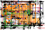
(b)

Figure 19: An illustration for the case considered in the reverse direction proof of Lemma 12. A path from $u_{4}$ to $\mathsf{nearY}(u_{1},d)$ (shown by $z$), to show that they are a pair of kitty corners, is drawn in orange.

Reduction Rule 9

Suppose that there exists a path $P=(u_{1},u_{2},u_{3},u_{4},u_{5},u_{6})$ in $G^{\rightarrow}$ such that $\mathsf{label}(u_{2})=\mathsf{label}(u_{5})=\mathsf{C}$ and $\mathsf{label}(u_{3})=\mathsf{label}(u_{4})=\mathsf{R}$. Then, delete the vertices $u_{3}$ and $u_{4}$ and the edges incident to them from $G^{\rightarrow}$ and add a new edge $(u_{2},u_{5})$ to $G^{\rightarrow}$. Moreover, assign $\mathsf{label}(u_{2})=\mathsf{label}(u_{5})=\mathsf{F}$, $\mathsf{weight}((u_{2},u_{5}))=\mathsf{weight}((u_{3},u_{4}))$ and $\mathsf{weight}((\mathsf{prev}(u_{1}),$ $u_{1}))=\max\{\mathsf{weight}((u_{2},$ $u_{3})),\mathsf{weight}((\mathsf{prev}(u_{1}),$ $u_{1}))\}$. The labels of all the remaining vertices and the weights of all the remaining edges stay the same. Let $G^{\rightarrow}_{\mathsf{red}}$ be the reduced graph.

Lemma 13

9 is safe.

Proof

The proof of the lemma follows the proof of Lemma 12.

Finally, to process a path labeled $\mathsf{RRRRRRR}$, we first define a matching $M_{RC}(G^{\rightarrow})$ from the $\mathsf{R}$-vertices to $\mathsf{C}$-vertices in $G^{\rightarrow}$ as follows. To define the matching, we first define the notion of a balanced path. Let $u$ and $v$ be two vertices of $G^{\rightarrow}$. We say that $P_{u,v}$ is balanced if the number of $\mathsf{R}$-vertices is equal to the number of $\mathsf{C}$-vertices in $P_{u,v}$. We have the following observation about a balanced path starting at an $\mathsf{R}$-vertex, which will be useful in defining the matching.

Observation 6

Let $P_{u,v}$ be a balanced path that starts with an $\mathsf{R}$-vertex. Then, there exists a $\mathsf{C}$-vertex $x$ on this path such that $P_{u,x}$ is balanced.

We now define the matching $M_{RC}(G^{\rightarrow})$. Intuitively, in $M_{RC}(G^{\rightarrow})$, every $\mathsf{R}$-vertex $u$ is matched to the closest $\mathsf{C}$-vertex $v$ such that every internal $\mathsf{R}$-vertex on the path from $u$ to $v$ is mapped to an internal $\mathsf{C}$-vertex on the path from $u$ to $v$. Formally, we define $M_{RC}(G^{\rightarrow})$ as a matching from the set of $\mathsf{R}$-vertices to the set of $\mathsf{C}$-vertices in $G^{\rightarrow}$ as follows.

An $\mathsf{R}$-vertex $u$ is matched to a $\mathsf{C}$-vertex $v$ if and only if i) $P_{u,v}$ is balanced, and ii) for every internal $\mathsf{C}$-vertex $x$ of $P_{u,v}$, the path $P_{u,x}$ is not balanced. Observe that as the number of $\mathsf{C}$-vertices is larger by $4$ than the number of $\mathsf{R}$-vertices, the matching $M_{RC}(G^{\rightarrow})$ always exists. Moreover, it is also unique. See Fig. 20. In the following lemma, we also prove that if an $\mathsf{R}$-vertex $u$ is matched to a $\mathsf{C}$-vertex $v$ then every $\mathsf{R}$-vertex on the path from $u$ to $v$ is matched to a $\mathsf{C}$-vertex on the path from $u$ to $v$.

Figure 20: An illustration for the definition of the matching $M_{RC}(G^{\rightarrow})$. The matched $\mathsf{R}$- and $\mathsf{C}$-vertex pairs are drawn in the same color and the remaining $4$ unmatched $\mathsf{C}$-vertices are drawn in black.

Lemma 14

Let $u$ be an $\mathsf{R}$-vertex in $G^{\rightarrow}$. Moreover, let $v$ be the $\mathsf{C}$-vertex in $G^{\rightarrow}$ that is matched to $u$ by $M_{RC}(G^{\rightarrow})$. Then, every $\mathsf{R}$-vertex on the path $P_{u,v}$ is matched to a $\mathsf{C}$-vertex on $P_{u,v}$ by $M_{RC}(G^{\rightarrow})$.

Proof

We prove the statement by induction on the number of vertices $\mathsf{num}$ of the path $P_{u,v}$. Observe that $\mathsf{num}$ is even as $P_{u,v}$ is balanced.

Base case $(\mathsf{num}=2)$. When $\mathsf{num}=2$, $P_{u,v}=(u,v)$ such that $\mathsf{label}(u)=\mathsf{R}$ and $\mathsf{label}(v)=\mathsf{C}$. As $u$ is matched to $v$, the lemma is true for $\mathsf{num}=2$.

Inductive hypothesis. Suppose that the lemma is true for $\mathsf{num}=2t\geq 2$.

Inductive step. We need to prove that the lemma is true for $\mathsf{num}=2t+2$. Let $P_{u,v}=(x_{1}=u,x_{2},\ldots,x_{2t+1},x_{2t+2}=v)$. Observe that $\mathsf{label}(x_{2})=\mathsf{R}$, otherwise $P_{u,x_{2}}$ is balanced, which contradicts property ii) of the definition of the matching. We now look at the path $P_{x_{2},x_{2t+1}}$. Since $P_{u,v}$ is balanced, $P_{x_{2},x_{2t+1}}$ is also balanced. Moreover, $\mathsf{label}(x_{2})=\mathsf{R}$; so, by 6, there exists a $\mathsf{C}$-vertex $x_{i}$, for some $i\in[2,2t+1]$, such that $P_{x_{2},x_{i}}$ is balanced. Let $j\geq 2$ be the smallest such index for which $P_{x_{2},x_{j}}$ is balanced and $\mathsf{label}(x_{j})=\mathsf{C}$. Due to the choice of $j$, for every internal $\mathsf{C}$-vertex $w$ of $P_{x_{2},x_{j}}$, the path $P_{x_{2},w}$ is not balanced. Therefore, by the definition of the matching, we get that $x_{2}$ is matched to $x_{j}$. As the the number of vertices of $P_{x_{2},x_{j}}$ is at most $2t$, from the inductive hypothesis, we get that every $\mathsf{R}$-vertex on $P_{x_{2},x_{j}}$ is matched to a $\mathsf{C}$-vertex on $P_{x_{2},x_{j}}$. Now, we remove the path $P_{x_{2},x_{j}}$ from $P_{u,v}$ and add an arc from $u$ to $x_{j+1}$. Let $P^{\prime}$ be the resulting path. Then, $P^{\prime}$ is balanced (since we removed a balanced path), and property ii) is also true for $P^{\prime}$ as it is true for $P_{u,v}$. Moreover, the number of vertices of $P^{\prime}$ is at most $2t$, so from the inductive hypothesis, we get the every $\mathsf{R}$-vertex on $P^{\prime}$ is matched to a $\mathsf{C}$-vertex on $P^{\prime}$. This, in turn, implies that every $\mathsf{R}$-vertex on $P_{u,v}$ is matched to a $\mathsf{C}$-vertex on $P_{u,v}$.

We now consider a path $(u_{1},u_{2},\ldots,u_{7})$ such that $\mathsf{label}(u_{i})=\mathsf{R}$, for every $i\in[1,7]$. Let $v_{i}$ be the $\mathsf{C}$-vertex that is matched to $u_{i}$ by $M_{RC}(G^{\rightarrow})$, for every $i\in[1,7]$. Observe that by the property i) of the definition of $M_{RC}(G^{\rightarrow})$, the number of $\mathsf{R}$-vertices is equal to the number of $\mathsf{C}$-vertices in $P_{u_{i},v_{i}}$ which implies that $\textrm{rot}(u_{i},v_{i})=-1$, for every $i\in[1,7]$. Moreover, by Lemma 14, $(u_{1},u_{2},u_{3},u_{4},u_{5},u_{6},u_{7},$ $\ldots,v_{7},\ldots,$ $v_{6},\ldots,$ $v_{5},\ldots,v_{4},\ldots,v_{3},\ldots,v_{2},\ldots,v_{1})$ is a path in $G^{\rightarrow}$. Therefore $\textrm{rot}(u_{1},v_{1})=\textrm{rot}(u_{1},u_{7})$ $+\textrm{rot}(u_{7},v_{7})+\textrm{rot}(v_{7},v_{1})$ $\Rightarrow$ $\textrm{rot}(v_{7},v_{1})=6$. As every $\mathsf{C}$-vertex is a reflex vertex on the outer face $f_{\textsf{out}}$ of $G^{\rightarrow}$, $\textrm{rot}(v_{1},v_{7})=-6$ on $f_{\textsf{out}}$. This, in turn, implies that $v_{1}$ and $v_{7}$ is a pair of kitty corners of $f_{\textsf{out}}$. Based on this matching $M_{RC}(G^{\rightarrow})$, we give the following counting rule to count the vertices of a path on $\mathsf{R}$-vertices having $7$ or more vertices.

Counting Rule 1

Let $k\in\mathbb{N}$ and $t\in[0,6]$. Let $P=(u_{1},u_{2},\cdot,u_{7k+t})$ be a maximal path on $\mathsf{R}$-vertices in $G^{\rightarrow}$ not containing any kitty corner, i.e., $\mathsf{label}(u_{i})=\mathsf{R}$ and $u_{i}$ is not a kitty corner of $H$, for every $i\in[7k+t]$. Let $v_{i}$ be the $\mathsf{C}$-vertex matched to $u_{i}$ by $M_{RC}(G^{\rightarrow})$. Then, we count the set of vertices of $P$ against the set of kitty corners $S_{P}=\{v_{1},v_{7},v_{8},v_{14},\ldots,v_{7k-6},v_{7k}\}$.

Note that, for every maximal path $P$ on $\mathsf{R}$-vertices having $7$ or more vertices, the set $S_{P}$ is unique. Moreover, if two such maximal paths $P_{1}$ and $P_{2}$ are different, then they are also vertex-disjoint and it holds that $S_{P_{1}}\cap S_{P_{2}}=\emptyset$. Therefore, by the above counting rule, the total number of occurrences of $\mathsf{R}$-vertices in $G^{\rightarrow}$ that belong to maximal paths $P$ on $\mathsf{R}$-vertices having $7$ or more vertices and not containing any kitty corner is bounded by a function that is linear in the number of kitty corners of $H$.

By applying Reduction Rules 1–9 in their respective order until they can no longer be applied, from 1, we get that $P^{\mathsf{trun}}_{c_{i},c_{i+1}}$ only contains $\mathsf{R}$-vertices and no kitty corner, for every $i\in[1,k]$. By applying 1, the number of vertices of all such paths is bounded by a function that is linear in the number of kitty corners of $H$. As the number of vertices of every path $P_{c_{i},c_{i+1}}$ is $10$ more than $P^{\mathsf{trun}}_{c_{i},c_{i+1}}$, we get an instance $I$ of the Weighted OC problem such that the number of vertices of $I$ is bounded by a function that is linear in the number of kitty corners of $H$. To show that it is a compression, we also need to prove that the sizes of the edge weights of $I$ (when encoded in binary) are bounded by a function that is linear in $k$. Observe that the weight of any edge of $I$ is at most $n$, the number of vertices of $G^{\rightarrow}$. Therefore, if the sizes of the edge weights of $I$ (when encoded in binary) are not bounded by a function that is linear in $k$, we get that $k=O(\log n)$. In this case, by Theorem 3.1, we can solve the OC problem on $G$ in $n^{O(1)}$ time. So, without loss of generality, we assume that $k=\Omega(\log n)$. This, in turn, implies that the size of $I$ is bounded by a function that is polynomial in the number of kitty corners of $H$. Thus we get a polynomial compression (with a linear number of vertices) parameterized by the number of kitty corners of $H$. Moreover, if $k=\Omega(\log n)$, the Weighted OC problem on cycle graphs is in NP due to the fact that we can always guess the length of each edge in the drawing (the number of guesses and the size of each number, that is, length, to guess are polynomial in $n$). As the OC problem on cycle graphs is NP-hard [22], we can exploit the following proposition given in the book of Fomin et al. [23] and conclude the proof of Theorem 4.1.

Proposition 1 ([23], Theorem 1.6)

Let $Q\subseteq\Sigma^{*}\times\mathbb{N}$ be a parameterized language, and let $R\subseteq\Sigma^{*}$ be a language such that the unparameterized version of $Q\subseteq\Sigma^{*}\times\mathbb{N}$ is NP-hard and $R\subseteq\Sigma^{*}$ is in NP. If there is a polynomial compression of $Q$ into $R$, then $Q$ admits a polynomial kernel.

Appendix 0.C Missing Proofs of Section 5

See 5.1

Proof

Let $\phi=({\cal X},{\cal C})$ be a SAT instance with variables ${\cal X}=X_{1},\ldots,X_{n}$ and clauses ${\cal C}=C_{1},\ldots,C_{m}$. Patrignani creates a graph $G_{\phi}$ with orthogonal representation $H_{\phi}$ and two variables $w_{\phi}=9n+4$ and $h_{\phi}=9m+7$ such that $H_{\phi}$ admits an orthogonal grid drawing of size $w_{\phi}\cdot h_{\phi}$ if and only if $\phi$ is satisfiable. On a high level, the reduction works as follows.

(a)

(b)

Figure 21: The shifting variable rectangles (shaded) and the belt (the path with hexagonal vertices) in the NP-hardness proof by Patrignani [30].

The outer face of $H_{\phi}$ (the frame) is a rectangle that requires width $w_{\phi}$ and height $h_{\phi}$ in its most compact drawing; see Fig. 21. Inside the frame, every variable is represented by a rectangular region (the variable rectangle of width 7 and height $h_{\phi}-7$. Each variable rectangle is bounded from above and below by a horizontal path, but not necessarily from the left and the right, as the clause gadgets will be laid through them. The variable rectangles are connected horizontally with hinges (short vertical paths) between them. Between the frame and the rectangles, there is a belt: a long path of $16n+4$ vertices that consists alternating subsequences of 4 reflex vertices followed by 4 convex vertices. The belt and the hinges make sure that every variable rectangle has to be drawn with exactly width 7 and height $h_{\phi}-7$, while the belt also ensures that every variable rectangle is either shifted to the top (which represents a $\mathsf{true}$ variable assignment) or to the bottom (which represents a $\mathsf{false}$ variable assignment) of the rectangle.

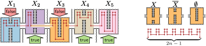
Figure 22: A clause gadget in the NP-hardness proof by Patrignani [30] for the clause $\overline{X_{1}}\vee X_{2}\vee\overline{X_{4}}$: the variable-clause rectangles (color shaded), the blocking rectangles (gray shaded), and the pathway (the path with diamond vertices). The segment that corresponds to a fulfilled variable assignment for this clause $(X_{2})$ is highlighted.

Every clause is represented by a chamber through the variable rectangles; see Fig. 22. The chambers divide the variable rectangles evenly into $m$ subrectangles of height 9, the variable-clause rectangles, with a height-2 connection between the rectangles; the height of the connection is ensured by further hinges above and below it. Depending on the truth-assignments of the variables, the variable-clause rectangles are either shifted up or shifted down by 3. Into each variable-clause rectangles, one or two blocker rectangles of width 1 are inserted, centered horizontally: if the corresponding variable does not appear in the clause, then a rectangle of height 7 at the top; if the variable appears negated, then a rectangle of height 2 at the top and a rectangle of height 5 at the bottom; and if the variable appears unnegated, then a rectangle of height 5 at the top and a rectangle of height 2 at the bottom. Into the chamber, a pathway that consists of $2n-1$ $\mathsf{A}$-shapes linked together by a horizontal segment is inserted. Each of the $\mathsf{A}$-shapes can reside in the left or right half of a variable-clause rectangle. Since there are $n$ variable-clause rectangles, one half of such a rectangle remains empty; hence, one horizontal segment of the pathway has to pass a blocker rectangle, one half of a variable-clause rectangle, and the connection between two variable-clause rectangles. Thus, there must be one variable-clause rectangle where the opening between the blocker rectangles and the opening to the previous/next variable-clause rectangle are aligned vertically, which is exactly the case if the corresponding variable fulfills its truth assignment in the corresponding clause. For a full reduction, see Fig. 23.

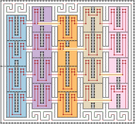
Figure 23: The full reduction by Patrignani [30] for the formula $(X_{2}\vee\overline{X_{4}})\wedge(X_{1}\vee X_{2}\vee\overline{X_{3}})\wedge(X_{5})\wedge(X_{4}\vee\overline{X_{5}})$ with variable assignment $X_{1}=X_{3}=\mathsf{false}$ and $X_{2}=X_{4}=X_{5}=\mathsf{true}$.

We now describe how to adjust the reduction such that every face has constant size, thus creating a graph $G^{\prime}_{\phi}$ that has a constant maximum face degree with orthogonal representation $H^{\prime}_{\phi}$ and two variables $w^{\prime}_{\phi}$ and $h^{\prime}_{\phi}$ such that $H^{\prime}_{\phi}$ admits an orthogonal grid drawing of size $w^{\prime}_{\phi}\cdot h^{\prime}_{\phi}$ if and only if $\phi$ is satisfiable.

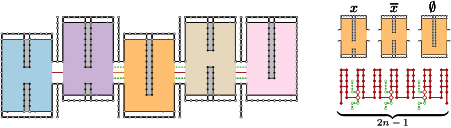
Figure 24: A clause gadget in our adjusted proof for the same clause and variable assignments as in Fig. 22.

We start with the clause gadgets. Observe that the chamber consists of two large faces of size $O(m)$: above the pathway and below the pathway. To avoid these large faces, we seek to connected the pathway to the boundary of each of the variable-clause rectangles; once at the top and once at the bottom; see Fig. 24. To achieve this, we first increase the width of all variable-clause rectangles by 2 and their height by 4. The height of the connection between the rectangles is increased to 4. In each variable-clause rectangle, the height of the top blocking rectangle is increased by 3, thus increasing the height of the opening between/below them to 3. The larger openings are required for the connections from the pathway to the boundary of the variable-clause rectangles. We have to make sure that the $\mathsf{A}$-shapes of the pathway still have to reside completely inside one half of a variable-clause rectangle. To achieve this, we also increase the necessary heights of the $\mathsf{A}$-shapes by adding to more vertices to the vertical segments of their top square. Now, the top part of each $\mathsf{A}$-shape is a rectangle of height at least 3, so it does not fit into any of the openings with size 3 or 4 without overlaps. We also add a vertex to the first and last vertical segment of the $\mathsf{A}$-shape that we will use to connect to the variable-clause rectangles later.

We seek to connect every second $\mathsf{A}$-shape to the top and bottom boundary of a variable-clause rectangle; namely, the $2i$-th $\mathsf{A}$-shape of the pathway shall be connected the the variable-clause rectangle corresponding to variable $X_{i}$, $1\leq i\leq n-1$. In particular, we always want to connect to the part to the right of the blocking rectangle. However, we do not know exactly which of the vertices to connect to, as it depends on whether the $\mathsf{A}$-shape is placed inside the same variable-clause rectangle or in the next one. Hence, We remove all vertices (except the corner vertices and those on the blocking rectangles) from the top and bottom boundary of the variable-clause rectangles, and add a single connector vertex between the right corner and the blocking rectangle, if it exists, or between the right and the left corner, otherwise. To make sure that the variable-clause rectangles still have the required width and that the blocking rectangles are placed in the middle, we add a path of length 11 (consisting of two vertical and nine horizontal segments) above and below the variable-clause rectangles, and connect the two middle vertices of the path to the blocking rectangle (if it exists).

Consider now the $2i$-th $\mathsf{A}$-shape and the $i$-th variable-clause gadget; refer again to Fig. 24. We connect the first vertex of the $\mathsf{A}$-shape to the bottom connector vertex by a path of length 3 that consists of a vertical downwards segment, followed by a horizontal leftwards segment and a vertical downwards segment. We connect the second vertex of the $\mathsf{A}$-shape to the top connector vertex by a path of length 2 that consists of a a horizontal leftwards segment followed by and a vertical upwards segment. If the $\mathsf{A}$-shape lies in the $i$-th variable clause gadget, then it lies in the right half of it. Since we increase the width of the rectangle, this half has width 3 and thus there is enough horizontal space for the connections if the $\mathsf{A}$-shape is drawn as far right as possible. Also, since the opening between/below the blocking rectangles has height 2, there is enough vertical space between the $\mathsf{A}$-shape and the bottom connector if the horizontal segment to the $(2i-1)$-th $\mathsf{A}$-shape is drawn as far up as possible. On the other hand, if the $\mathsf{A}$-shape lies in the $(i+1)$-th variable clause gadget, then it lies in the left half of it. Since the opening between the variable-clause rectangles now has height 3, there is enough vertical space to fit the the connection to the $(2i-1)$-th $\mathsf{A}$-shape as well as the horizontal segment on the path to the connector vertices through the opening, and if the $\mathsf{A}$-shape that lies in the right half of the $i$-th variable-clause rectangle is drawn as far left as possible, then there is also enough horizontal space to fit the vertical connection.

We still have to make sure that one half of a variable-clause rectangle can be “skipped” by the pathway if and only if the truth-assignment of a variable is fulfilled in the corresponding clause. We increase the lengths of the top hinges by 3 and the lengths of the bottom hinges by 1. This ensures that the opening of the connections has height 4 as required, and that horizontal segment can pass though a connection and a blocking rectangle opening if and only if a variable is variable rectangle is shifted down (the variable is assigned $\mathsf{false}$) and the variable appears negated in the clause, or if a variable is shifted up (the variable is assigned $\mathsf{false}$) and the variable appears unnegated in the clause, therefore satisfying our requirements. Furthermore, observe that all faces in the clause gadget now have degree at most 5: there are at most 25 vertices from the pathway (2 $\mathsf{A}$-shapes + 1 vertex), at most 18 vertices from a blocking rectangle, at most 6 vertices from the paths to (including) the connector vertices, and at most 6 vertices from the boundary of the chamber.

We now consider the frame and the variable rectangles. There are three large faces: the outer face, the face between the frame and the belt, and the face between the belt and the variable rectangles; all of these have degree $\Theta(n+m)$.

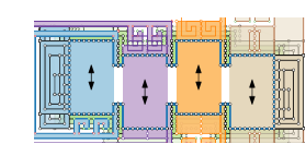
(a)

(b)

Figure 25: The frame in our adjusted NP-hardness reduction. (a) The left and right extensions of the first and last variable rectangle; (b) the belts around the variable rectangles.

We first show how to deal with the face between the variable rectangles and the belt. We ignore the belt for now and focus on the path around the variable rectangles; see Fig. 25. This path consists of two vertical paths length $O(m)$ on the left and the right of the first and the last variable rectangle, respectively, and an $x$-monotone path of length $O(n)$ between them. Consider the vertical path on the left of the first variable rectangle, let $z\in O(m)$ be its length and pick some constant integer $c\geq 2$. We first place a rectangle to the left of path by connecting the topmost with the bottommost vertex with a path of length 3, consisting of a horizontal leftward segment followed by a vertical downward and a horizontal rightward segment. This creates a new interior rectangular face with 2 vertices on the left and $z$ vertices on the right. We now iteratively decrease the degree of this face, adding new faces of degree 10 and rectangular faces of degree at most $c+3$, until this face also has constant degree. We place at most $z/c$ rectangles to the left of the right path, each of height at most $c$, by adding a vertical path of at most $z/c+1$ vertices that are connected to the second vertex from the top, the second vertex from the bottom, and every $c$-th vertex in between. This way, we create at most $z/c$ new faces of degree at most $c+3$, and a new vertical path of length at most $z/c+1$. We connect the topmost and the bottommost vertex of this new path to create a new rectangular face as before. This creates a C-shaped face of degree 10, and a new interior rectangular face with two vertices on the left and at most $z/c+1$ vertices on the right. We repeat this process at most $\log_{c}(z)+1$ times, until the vertical path on the right has length at most $c$ and thus the interior face has degree at most $c+6$; see Fig. 25(a). We do the same to the vertical path on the right of the last variable rectangle. This way, we create at most $2z$ new faces, all constant degree, and the full path now has length $O(n)$.

Instead of placing a single belt and outer face, we now add a small belt of only 20 vertices around every variable rectangle. Namely, the belt starts and ends at the rightmost vertex of the top and bottom boundary of the variable rectangles, respectively. For the first variable rectangle, the belt bounds a face of at most $30+c$ vertices: 20 from the belt, 10 from the top, and $c$ from the extension to the left. We add another path between the extreme vertices of the hinges between the variable rectangles that consists of four $90^{\circ}$-vertices; this creates a face of degree 40: 4 from this path, 20 from the belt, 10 from the hinges, and 6 from the variable rectangles. This path also functions as a bounding box for the belt: the minimum bounding box for this path can only be achieved if both spirals of the belt are either below or above the variable rectangle, thus creating the binary choice of shifting the variable rectangle up ($\mathsf{true}$) or down ($\mathsf{false}$).

For the next variable rectangles, we have to be a bit more careful. Repeating the process as for the first variable rectangle does not immediately work, as the new belt has to walk around the path that describes the bounding box for the previous variable rectangle plus its belt. Thus, there would be a gap of height 2 above and below the variable rectangle. This means that the variable rectangle could shift up- and downwards by two coordinates, which makes the clause gadgets invalid. To avoid this issue and to close the gap, we place a box of height 2 above and below the second variable rectangle, and we place a box of height $2(i-1)$ around the $i$-th variable rectangle, for each $i\in\{3,\dots,n\}$. To avoid a face of degree $O(n)$, we use the same strategy as for the leftmost path of the left variable gadget: we place a rectangle with an interior vertical path of height $2(i-1)$ and we keep refining the resulting faces until they all have constant degree. This way, we create $2(n-1)$ faces of degree at most 46: 20 from the belt, 4 from the bounding box path, 10 from the hinges, 6 from the vertical extension boxes, and 6 from the variable rectangles. The outer face of the graph has only degree 6: four from the bounding box, and the two corners of the rightwards extension of the last variable rectangle.

With this adjustment, we can still encode the variable assignments of a variable rectangle being either shifted up ($\mathsf{true}$) or down ($\mathsf{false}$), and we can draw the orthogonal representation with minimum width and height if and only if every clause gadget has a compact drawing, thus the whole orthogonal representation has an orthogonal drawing with area $w^{\prime}_{\phi}\times h^{\prime}_{\phi}$ for some fixed width $w^{\prime}_{\phi}$ and height $h^{\prime}_{\phi}$ if and only if $\phi$ is satisfyable. Clearly, $w^{\prime}_{\phi}$ and $h^{\prime}_{\phi}$ (and the number of vertices) are polynomial in $n$ and $m$, and as described above all faces have constant degree.

Hence, OC remains NP-hard even for graphs of constant face degree and thus it is para-NP-hard when parameterized by the maximum face degree.

Appendix 0.D Missing Proofs of Section 6

See 6.1

Proof

Let $H$ be the given orthogonal representation, let $G$ be the underlying connected graph, let $n$ be the number of vertices of $G$, let $b$ the total number of edge bends in $H$, and let $h\geq 1$ be an integer. We want to decide, in $(O(n+b))^{O(h)}$ time, whether $H$ admits an orthogonal drawing on a grid that consists of $h$ horizontal lines. Given a solution, that is, a drawing of $H$, we can remove any column that does not contain any vertex or bend point. Hence it suffices to check whether there exists a drawing of $H$ on a grid of (height $h$ and) width $w\leq n+b$.

To this end, we use dynamic programming (DP) with a table $B$. Each entry of $B[c,t]$ corresponds to a column $c$ of the grid and an $h$-tuple $t$. For an example, see Fig. 26. Each component of $t$ represents an object (if any) that lies on the corresponding grid point in column $c$. In a drawing of $H$, a grid point $g$ can either be empty or it is occupied by a vertex or by an edge. In the case of an edge, the edge can pass through $g$ either horizontally or vertically, or it can have a bend point at $g$, as prescribed by $H$. Let $\mathcal{T}$ be the set of $h$-tuples constructed in this way. Due to our observation regarding $w$ above, $\mathcal{T}$ does not contain any $h$-tuple that consists exclusively of horizontally crossing edges and empty grid points. Note that $|\mathcal{T}|\in(O(n+b))^{h}$.

Observe that, in an orthogonal drawing, each column can be considered a cut of the graph that the drawing represents. Hence, any $t\in\mathcal{T}$ uniquely defines all elements of $H$ that, in any height-$h$ grid drawing, cross $c$ or lie to the left of $c$. We refer to this part of $H$ as $\mathsf{left}_{H}(t)$. Analogously, we define the set $\mathsf{on}(t)$ as the elements that are encoded by $t$, that is, vertices or edges of $H$ that lie on the corresponding grid column, or edges that cross the column or have a bend point on it. The table entry $B[c,t]$ stores a Boolean value that is true if an orthogonal drawing of $\mathsf{left}_{H}(t)$ on a grid of size $c\times h$ (counting grid lines) exists, false otherwise.

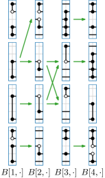
Figure 26: Part of the DP table for checking whether the orthogonal representation depicted in Figs. 1(a) and 1(b) admits a drawing of height 5. The arcs that enter an entry $B[c,t]$ come from the entries that are taken into account when computing $B[c,t]$.

We construct our drawing from left to right. Let $c\in\{1,\dots,w\}$ be the index of the current grid column. If $c=1$, we check, for each $t\in\mathcal{T}$ whether $\mathsf{left}_{H}(t)=\emptyset$. In this case, we set $B[c,t]=\mathsf{true}$, otherwise to $\mathsf{false}$. If $c>1$, we check for each $t\in\mathcal{T}$, whether $t$ can be extended to the left by one unit. We do this as follows. Let $t^{\prime}\in\mathcal{T}$ be a direct predecessor of $t$ if $\mathsf{left}_{H}(t)=\mathsf{left}_{H}(t^{\prime})\cup\mathsf{on}(t^{\prime})$ and, if we place $t^{\prime}$ on a column directly in front of $t$, they “match”, that is, every edge that starts in $t^{\prime}$ or crosses $t^{\prime}$ either ends on $t$ or crosses $t$ (and vice versa). In particular, edges that cross both columns must lie in the same row. We set $B[c,t]=\mathsf{true}$ if $t$ has a direct predecessor $t^{\prime}$ such that $B[c-1,t^{\prime}]=\mathsf{true}$. Otherwise we set $B[c,t]=\mathsf{false}$.

The DP returns $\mathsf{true}$ if and only if, for any $c\in\{1,\dots,w\}$ and $t\in\mathcal{T}$, it holds that $B[c,t]=\mathsf{true}$ and $\mathsf{left}_{H}(t)\cup\mathsf{on}(t)=V(H)\cup E(H)$.

The number of different $h$-tuples is $(O(n+b))^{h}$. For each $c\in\{1,\dots,w\}$ and $t\in\mathcal{T}$, we can compute $B[c,t]$ in $(h\cdot O(n+b))^{h}$ time. Hence, the DP runs in $(O(n+b))^{O(h)}$ total time.

References

- [1] M. J. Bannister, S. Cabello, and D. Eppstein. Parameterized complexity of 1-planarity. J. Graph Algorithms Appl., 22(1):23–49, 2018. doi:10.7155/jgaa.00457.
- [2] M. J. Bannister and D. Eppstein. Crossing minimization for 1-page and 2-page drawings of graphs with bounded treewidth. J. Graph Algorithms Appl., 22(4):577–606, 2018. doi:10.7155/jgaa.00479.
- [3] M. J. Bannister, D. Eppstein, and J. A. Simons. Inapproximability of orthogonal compaction. J. Graph Algorithms Appl., 16(3):651–673, 2012. doi:10.7155/jgaa.00263.
- [4] M. J. Bannister, D. Eppstein, and J. A. Simons. Fixed parameter tractability of crossing minimization of almost-trees. In S. Wismath and A. Wolff, editors, Int. Symp. Graph Drawing (GD), volume 8242 of LNCS, pages 340–351. Springer, 2013. doi:10.1007/978-3-319-03841-4_30.
- [5] J. L. Bentley and T. Ottmann. Algorithms for reporting and counting geometric intersections. IEEE Transactions on Computers, C-28(9):643–647, 1979. doi:10.1109/TC.1979.1675432.
- [6] P. Bertolazzi, G. Di Battista, G. Liotta, and C. Mannino. Upward drawings of triconnected digraphs. Algorithmica, 12(6):476–497, 1994. doi:10.1007/BF01188716.
- [7] S. Bhore, R. Ganian, F. Montecchiani, and M. Nöllenburg. Parameterized algorithms for book embedding problems. J. Graph Algorithms Appl., 24(4):603–620, 2020. doi:10.7155/jgaa.00526.
- [8] S. Bhore, R. Ganian, F. Montecchiani, and M. Nöllenburg. Parameterized algorithms for queue layouts. In D. Auber and P. Valtr, editors, Int. Symp. Graph Drawing & Network Vis. (GD), volume 12590 of LNCS, pages 40–54. Springer, 2020. doi:10.1007/978-3-030-68766-3_4.
- [9] T. C. Biedl. Small drawings of outerplanar graphs, series-parallel graphs, and other planar graphs. Discret. Comput. Geom., 45(1):141–160, 2011. doi:10.1007/s00454-010-9310-z.
- [10] C. Binucci, G. Da Lozzo, E. Di Giacomo, W. Didimo, T. Mchedlidze, and M. Patrignani. Upward book embeddings of st-graphs. In Symp. Comput. Geom. (SoCG), volume 129 of LIPIcs, pages 13:1–13:22. Schloss Dagstuhl – Leibniz-Zentrum für Informatik, 2019. doi:10.4230/LIPIcs.SoCG.2019.13.
- [11] S. S. Bridgeman, G. Di Battista, W. Didimo, G. Liotta, R. Tamassia, and L. Vismara. Turn-regularity and optimal area drawings of orthogonal representations. Comput. Geom., 16(1):53–93, 2000. doi:10.1016/S0925-7721(99)00054-1.
- [12] S. Chaplick, E. Di Giacomo, F. Frati, R. Ganian, C. N. Raftopoulou, and K. Simonov. Parameterized algorithms for upward planarity. arXiv, 2022. doi:10.48550/arXiv.2203.05364.
- [13] S. Chaplick, K. Fleszar, F. Lipp, A. Ravsky, O. Verbitsky, and A. Wolff. Drawing graphs on few lines and few planes. J. Comput. Geom., 11(1):433–475, 2020. doi:10.20382/jocg.v11i1a17.
- [14] M. Cygan, F. V. Fomin, L. Kowalik, D. Lokshtanov, D. Marx, M. Pilipczuk, M. Pilipczuk, and S. Saurabh. Parameterized Algorithms. Springer, 2015.
- [15] G. Da Lozzo, D. Eppstein, M. T. Goodrich, and S. Gupta. Subexponential-time and FPT algorithms for embedded flat clustered planarity. In Int. Workshop on Graph-Theoretic Concepts in Computer Science (WG), volume 11159 of LNCS, pages 111–124. Springer, 2018. doi:10.1007/978-3-030-00256-5_10.
- [16] G. Di Battista, P. Eades, R. Tamassia, and I. G. Tollis. Graph Drawing: Algorithms for the Visualization of Graphs. Prentice-Hall, 1999.
- [17] G. Di Battista and R. Tamassia. Algorithms for plane representations of acyclic digraphs. Theor. Comput. Sci., 61:175–198, 1988. doi:10.1016/0304-3975(88)90123-5.
- [18] E. Di Giacomo, G. Liotta, and F. Montecchiani. Orthogonal planarity testing of bounded treewidth graphs. J. Comput. Syst. Sci., 125:129–148, 2022. doi:10.1016/j.jcss.2021.11.004.
- [19] R. G. Downey and M. R. Fellows. Fundamentals of Parameterized Complexity, volume 4 of TCS. Springer, 2013. doi:10.1007/978-1-4471-5559-1.
- [20] V. Dujmović, M. R. Fellows, M. Kitching, G. Liotta, C. McCartin, N. Nishimura, P. Ragde, F. A. Rosamond, S. Whitesides, and D. R. Wood. On the parameterized complexity of layered graph drawing. Algorithmica, 52(2):267–292, 2008. doi:10.1007/s00453-007-9151-1.
- [21] V. Dujmović, H. Fernau, and M. Kaufmann. Fixed parameter algorithms for one-sided crossing minimization revisited. J. Discrete Algorithms, 6(2):313–323, 2008. doi:10.1016/j.jda.2006.12.008.
- [22] W. S. Evans, K. Fleszar, P. Kindermann, N. Saeedi, C.-S. Shin, and A. Wolff. Minimum rectilinear polygons for given angle sequences. Comput. Geom., 100(101820):1–39, 2022. doi:10.1016/j.comgeo.2021.101820.
- [23] F. V. Fomin, D. Lokshtanov, S. Saurabh, and M. Zehavi. Kernelization: Theory of Parameterized Preprocessing. Cambridge University Press, 2019.
- [24] R. Ganian, F. Montecchiani, M. Nöllenburg, and M. Zehavi. Parameterized complexity in graph drawing (Dagstuhl Seminar 21293). Dagstuhl Reports, 11(6):82–123, 2021. doi:10.4230/DagRep.11.6.82.
- [25] S. Gupta, G. Sa’ar, and M. Zehavi. Grid recognition: Classical and parameterized computational perspectives. In Int. Symp. Algorithms & Comput. (ISAAC), volume 212 of LIPIcs, pages 37:1–37:15. Schloss Dagstuhl – Leibniz-Zentrum für Informatik, 2021. doi:10.4230/LIPIcs.ISAAC.2021.37.
- [26] M. Kaufmann and D. Wagner, editors. Drawing Graphs, Methods and Models, volume 2025 of Lecture Notes in Computer Science. Springer, 2001. doi:10.1007/3-540-44969-8.
- [27] Y. Kobayashi, H. Ohtsuka, and H. Tamaki. An improved fixed-parameter algorithm for one-page crossing minimization. In D. Lokshtanov and N. Nishimura, editors, 12th Int. Symp. Parametr. & Exact Comput. (IPEC), volume 89 of LIPIcs, pages 25:1–25:12. Schloss Dagstuhl – Leibniz-Zentrum für Informatik, 2018. doi:10.4230/LIPIcs.IPEC.2017.25.
- [28] G. Liotta, I. Rutter, and A. Tappini. Parameterized complexity of graph planarity with restricted cyclic orders. In Int. Workshop on Graph-Theoretic Concepts in Computer Science (WG), volume 13453 of LNCS, pages 383–397. Springer, 2022. doi:10.1007/978-3-031-15914-5_28.
- [29] G. D. Lozzo, D. Eppstein, M. T. Goodrich, and S. Gupta. C-planarity testing of embedded clustered graphs with bounded dual carving-width. Algorithmica, 83(8):2471–2502, 2021. doi:10.1007/s00453-021-00839-2.
- [30] M. Patrignani. On the complexity of orthogonal compaction. Comput. Geom., 19(1):47–67, 2001. doi:10.1016/S0925-7721(01)00010-4.
- [31] C. A. Pickover. The Math Book. Sterling, 2009.
- [32] M. I. Shamos and D. Hoey. Geometric intersection problems. In 17th Ann. Symp. Foundat. Comput. Sci. (FOCS), pages 208–215, 1976. doi:10.1109/SFCS.1976.16.
- [33] R. Tamassia. On embedding a graph in the grid with the minimum number of bends. SIAM J. Comput., 16(3):421–444, 1987. doi:10.1137/0216030.