Density of instantaneous frequencies in the Kuramoto-Sakaguchi model

Abstract

We obtain a formula for the statistical distribution of instantaneous frequencies in the Kuramoto-Sakaguchi model. This work is based on the Kuramoto-Sakaguchi’s theory of globally coupled phase oscillators, which we review in full detail by discussing its assumptions and showing all steps behind the derivation of its main results. Our formula is a stationary probability density function with a complex mathematical structure, is consistent with numerical simulations and gives a description of the stationary collective states of the Kuramoto-Sakaguchi model.

¹ Departamento de Física, Universidade Estadual Paulista, Bela Vista, 13506-900 Rio Claro, SP, Brazil

² Departamento de Física, Universidade Federal de São Paulo, UNIFESP, 09913-030, Campus Diadema, São Paulo, Brasil

1 Introduction

Synchronization is the process by which interacting oscillatory systems adjust their frequencies in order to display the same common value [1]. Power grids [2], semiconductor laser arrays [3], cardiac pacemaker cells [4], and neurosciences [5] are just a few examples in a multitude of domains where synchronization is an active research subject.

The works of A. Winfree and Y. Kuramoto brought seminal contributions to the study of synchronization [4, 6, 7, 8]. Inspired by Winfree’s pioneering ideas [9], Kuramoto formulated a model of coupled phase oscillators today known as Kuramoto model. The Kuramoto model was introduced in Ref. [7], and its first and more detailed analysis by Kuramoto himself, published in Ref. [8]. Since then, many studies about the Kuramoto model and its variants appeared in the literature. (Reviews about the Kuramoto model can be found in Refs. [10, 11]; see Refs. [12, 13, 14, 15] for later studies related to variants of the Kuramoto model and their applications.)

The Kuramoto model consists of an ensemble of oscillators with a mean-field coupling and randomly distributed natural (or intrinsic) frequencies. An oscillator is characterized by its phase, and the first-order time derivative of the oscillator’s phase, which here we call instantaneous frequency, is defined by an autonomous first-order ordinary differential equation. The theoretical analysis of the Kuramoto model [8, 11] evinces a transition between two stationary collective states: an incoherent state and a synchronization one. In the incoherent state, instantaneous and natural frequencies have the same statistical distribution. In the synchronization state, some oscillators have instantaneous frequencies sharing the same value. The number of synchronized oscillators depends on the model’s parameter called coupling-strength, and synchronization only occurs for a coupling strength above a critical value [8, 11]. In a simplified version of the Kuramoto model, identical (with the same natural frequencies) and symmetrically-coupled oscillators show multiple regular attractors [16], and the synchronization state is the most probable one[17, 18].

H. Sakaguchi and Y. Kuramoto created a generalization of the Kuramoto model [19] introducing into the coupling function a phase shift, also called phase-lag. The Kuramoto-Sakaguchi model and its variants appear in the study of a wide range subjects such as chimera states [20, 21], chaotic transients [22], pulse-coupled oscillators [23], and Josephson-junction arrays [24]. In addition, the coupling function with a phase-lag can be interpreted as an approximate model of interactions with time-delayed phases [25]. The Kuramoto-Sakaguchi model exhibits the same stationary collective states as the original Kuramoto model [19].

Collective states of Kuramoto-like models are commonly characterized by means of an order parameter, which is zero in the incoherent state and takes finite values in the synchronization state. In this work, we follow a different approach from the usual order-parameter analysis uncovering how instantaneous frequencies are statistically distributed in the stationary collective states of the Kuramoto-Sakaguchi model. Instantaneous frequencies collectively reflect the occurence of synchronized behavior [26], and they are also relevant in the study of other phenomena (e.g. frequency spirals [32]).

We will show how to obtain a formula for the statistical distribution of instantaneous frequencies. The formula is defined by a stationary probability density function, which we refer to as density of instantaneous frequencies. Our goal is similar to the one pursued in Ref. [26] for the Kuramoto model, but here we will show how to obtain a more general result in a more straightforward way. A related (but still rather a different) problem was addressed by Sakaguchi and Kuramoto in Ref. [19], where they analyzed the statistical distribution of coupling-modified frequencies, namely instantaneous frequencies averaged over infinitely large time intervals (see Refs. [11, 26] for further details).

This work is based on the Kuramoto-Sakaguchi theory, described, as far as we know, only in Ref. [19]. We will discuss the fundamental assumptions of the Kuramoto-Sakaguchi theory and detail how its main results can be derived. Our opinion is that an explicit presentation of the Kuramoto-Sakaguchi theory is still absent.

We organized this paper as follows. In Section 2, we present the Kuramoto-Sakaguchi theory and state diagrams pointing out the transition between the incoherent and synchronization states. In Section 3, we extend the Kuramoto-Sakaguchi theory by providing additional analytical results and obtaining the formula of the density of instantaneous frequencies. In Section 4, we discuss the properties of our formula in a specific application example, in which natural frequencies have a Gaussian statistical distribution. In Section 5, we check the consistency of our formula with numerical simulation data. Conclusions and an outlook on possible research directions are given in Section 6.

2 Kuramoto-Sakaguchi theory

The Kuramoto-Sakaguchi (KS) model[19] consists of an infinitely large number $N$ of all-to-all coupled oscillators. The state of an oscillator of index $i=1...N$ is characterized by its phase $\theta_{i}$, which changes in time according to

$$\dot{\theta_{i}}=\omega_{i}-\frac{K}{N}\sum_{j=1}^{N}\sin(\theta_{i}-\theta_{j}+\alpha),$$ (1)

where $\dot{\theta_{i}}$ is the first-order time-derivative of $\theta_{i}$, $\omega_{i}$ is a random number with a prescribed density, and $K$ and $\alpha$ are real constant parameters. We refer to $\dot{\theta_{i}}$ as the instantaneous frequency, $\omega_{i}$ is called natural frequency and $K$, the coupling strength. The oscillator of index $j$ can be represented by the complex number $\exp(i\theta_{j})$. Oscillators are then points in a complex plane moving over a unit-radius circle centered at the origin.

A valuable concept for the analysis of collective behavior in the KS model is that of mean field, defined by

$$Z=\frac{1}{N}\sum_{j=1}^{N}\exp(i\theta_{j}),$$ (2)

which can be interpreted as the average oscillator state. The mean field can be written as a complex number

$$Z=R\exp(i\Theta)$$ (3)

where $\Theta$ denotes the mean-field phase and $R$, the mean-field modulus, referred to as order parameter. If the oscillators are quasi-aligned, i.e., they have approximately the same phase, then $R\simeq 1$. Yet, a quasi-uniform scattering of all oscillator-points over the circle results in a mean-field located near the origin, i.e. $R\simeq 0$.

For $N\longrightarrow\infty$, the mean field, at a time instant $t$, is given by

$$Z=\intop_{-\pi}^{+\pi}\exp(i\theta)n(\theta,t)d\theta,$$ (4)

where $n(\theta,t)$ is the density of phases at the same time instant. Two simple scenarios are assumed concerning the properties of $n(\theta,t)$ in the long-time ($t\longrightarrow\infty$) and large-size ($N\longrightarrow\infty$) limits. First, $n(\theta,t)=\frac{1}{2\pi}$ for $-\pi<\theta\leq+\pi$, and $n(\theta,t)=0$, otherwise, i.e. $n(\theta,t)$ is a time-independent and uniform density (the value $\frac{1}{2\pi}$ comes from the normalization condition). Second, $n(\theta,t)$ is a steadily traveling wave with velocity $\Omega$, i.e. $n(\theta-\Omega\Delta t,t)=n(\theta,t+\Delta t)$ for any time instant $t$ and time interval $\Delta t$. This means that the wave profile does not change in time, and the wave propagates with constant-in-time velocity $\Omega$. We call the wave-propagation velocity, $\Omega$, synchronization frequency.

The first scenario defines the incoherent state, and the second, the synchronization state. In the incoherent state, oscillators are uniformly spread over the unit circle. In the synchronization state, a bunch of oscillators is synchronized, that is, they change collectively their phase at the same constant rate $\Omega.$

After inserting a uniform phase density in Eq. (4), we see that $Z=0$. So, from Eq. (3), the order parameter ($R$) is zero in the incoherent state. Yet, if a KS system exhibits synchronization, then the assumption of a traveling wave with a stationary and non-uniform profile, moving with constant velocity $\Omega$, means that $R$ is finite and time-independent. Moreover, $Z$ moves in the complex plane following a circular path of radius $R$ and velocity $\Omega$. That is, a uniform circular motion given by

$$Z(t)=R\exp\left[i\left(\Omega t+\Theta_{0}\right)\right],$$ (5)

where $\Theta_{0}$ is the mean-field phase at an arbitrary initial time instant.

Let us consider KS oscillators in a different complex plane, with the same origin as the previous one, but with both axis rotating with angular velocity $\Omega$. In the new rotating frame, we represent the oscillator of index $j$ by the complex number $\exp(i\psi_{j})$, where $\psi_{j}$ is the oscillator’s phase. The analogous of Eqs. (2), (3), and (4) are

$$Z^{{}^{\prime}}=\frac{1}{N}\sum_{j=1}^{N}\exp(i\psi_{j}),$$ (6)

$$Z^{\prime}=R\exp(i\Psi),$$ (7)

and, for $N\longrightarrow\infty$,

$$Z^{{}^{\prime}}=\intop_{-\pi}^{+\pi}\exp(i\psi)n(\psi)d\psi.$$ (8)

The quantities $Z^{{}^{\prime}}$ and $n(\psi)$ are representations of the mean field and the phase density in the rotating frame. Comparing Eq. (3) to Eq. (7), we see that $Z$ and $Z^{\prime}$ have the same length $R$. The mean-field length is invariant to the change of frames because the phase density profile is kept unchanged. Note also that, in Eq. (8), we removed the time dependence from the phase density, since both the rotating frame and the steadily traveling wave move together with the same velocity $\Omega$. So, both $R$ and $\Psi$ are time-independent, which is the same as stating that the mean field is fixed in the rotating frame.

Some conventions are useful to simplify the analysis of the KS model at a time instant $t>t_{o}=0$, with $t_{0}$ denoting the initial time instant. We choose a fixed frame such that its real axis has the same direction as the mean field at time $t_{0}$. So, $\Theta_{0}=0$ and $Z(0)=R$. Another important convention is defining a rotating frame such that, at the initial time $t_{0}$, its real axis is dephased by $\alpha$ from the fixed-frame’s real axis (the same parameter $\alpha$ of Eq. (1)). This is the same as setting $\Psi=\alpha$.

Thus, from Eqs. (5) and (7), at the time instant $t$,

$$Z(t)=R\exp\left(i\Omega t\right)$$ (9)

and

$$Z^{\prime}=R\exp i\alpha.$$ (10)

Also, as a consequence of the above conventions, a simple geometric inquiring yields the relations

$$\dot{\psi_{i}}=\dot{\theta_{i}}-\Omega$$ (11)

and

$$\psi_{i}=\theta_{i}-\Omega t+\alpha.$$ (12)

In Eq. (11), $\dot{\psi_{i}}$ is the instantaneous frequency of an oscillator of index $i$ in the rotating frame.

Using Eqs. (11) and (12), we can recast Eq. (1) as

$$\dot{\psi_{i}}=\omega_{i}-\Omega-\frac{K}{N}\sum_{j=1}^{N}\sin(\psi_{i}-\psi_{j}+\alpha).$$ (13)

Multiplying the right-hand sides of Eqs. (6) and (10) by $\exp\left[-i\left(\psi_{i}+\alpha\right)\right]$ and equating their imaginary parts result in

$$N^{-1}\sum_{j=1}^{N}\sin(\psi_{i}-\psi_{j}+\alpha)=R\sin\psi_{i}.$$ (14)

Substituting the summation in Eq. (13) by the right-hand-side of Eq. (14) gives

$$\dot{\psi_{i}}=\omega_{i}-\Omega-KR\sin\psi_{i},$$ (15)

which is a simple formulation of the KS model in the rotating frame. We emphasize that $\omega_{i}$, $K$, $\Omega$, and $R$ are constant-in-time numbers: $\omega_{i}$ is a sample from a random variable with a given probability density function $g$; $K$ is a given coupling strength; $\Omega$ and $R$ are constants to be determined.

The differential equation (15) gives a more detailed picture of synchronization in the KS model. For $\left|\omega_{i}-\Omega\right|>KR$, Eq. (15) has no equilibrium point. When $\left|\omega_{i}-\Omega\right|=KR$, a pair of stable and unstable equilibria emerges by a fold bifurcation, and they become apart as $\left|\omega_{i}-\Omega\right|<KR$. Since the phase domain is closed ($\left|\psi_{i}\right|\leq\pi$), the phase of an oscillator $i$, for which $\left|\omega_{i}-\Omega\right|\leq KR$, will always converge to an attractor (stable equilibrium point) defined by

$$\psi_{i}^{*}=\sin^{-1}\left(\frac{\omega_{i}-\Omega}{KR}\right),$$ (16)

where $\sin^{-1}$ is an inverse of the $sin$ function with domain $\left[-1,+1\right]$ and image $\left[-\frac{\pi}{2},+\frac{\pi}{2}\right]$. Then, $-\frac{\pi}{2}\leq\psi_{i}^{*}\leq+\frac{\pi}{2}$.

The latter case, where oscillator $i$ has a natural frequency such that $-KR+\Omega\leq\omega_{i}\leq\Omega+KR$, means, according to Eqs. (11), (12), (15), and (16), that $\psi_{i}\longrightarrow\psi_{i}^{*}$, $\theta_{i}\longrightarrow\psi_{i}^{*}+\Omega t-\alpha$, $\dot{\psi_{i}}\longrightarrow 0$, and $\dot{\theta_{i}}\longrightarrow\Omega$ as $t\longrightarrow+\infty$. This is the case of a synchronized oscillator, or, following Kuramoto’s terminology, an S oscillator. But, for $\left|\omega_{i}-\Omega\right|>KR$, i.e, oscillator $i$ has a natural frequency such that $\omega_{i}<-KR+\Omega$ or $\Omega+KR<\omega_{i},$ Eq. (15) has no equilibrium point. Then, oscillator-$i$’s phase varies according to Eq. (15) without slowing down towards an asymptotic value. This is a desynchronized oscillator, or, simply, a D oscillator.

Let $n(\psi,\omega)$ denote the joint density for a rotating-frame phase $\psi$ and a natural frequency $\omega$. The associated marginal phase density is given by

$$n(\psi)=\intop_{-\infty}^{+\infty}n(\psi,\omega)\,d\omega,$$ (17)

where $-\pi<\psi\leq+\pi$. Eq. (17) can be rewritten as

$$n(\psi)=\intop_{\left|\omega-\Omega\right|\leq KR}n(\psi,\omega)\,d\omega+\intop_{\left|\omega-\Omega\right|>KR}n(\psi,\omega)\,d\omega.$$ (18)

The first term in the right-hand side of Eq. (18) is the phase density for S oscillators, and the second one, the phase density for D oscillators. The two terms are functions of $\psi$ which we denote by $n_{S}(\psi)$ and $n_{D}(\psi)$, respectively. Then,

$$n(\psi)=n_{S}(\psi)+n_{D}(\psi).$$ (19)

Let $n(\psi|\omega)$ be the conditional phase density for a given natural frequency $\omega$. If $g(\omega)$ is the natural-frequency density, replacing $n(\psi,\omega)$ with $n(\psi|\omega)g(\omega)$ leads to

$$n_{S}(\psi)=\intop_{\Omega-KR}^{\Omega+KR}n_{S}(\psi|\omega)g(\omega)\,d\omega$$ (20)

and

$$n_{D}(\psi)=\intop_{-\infty}^{\Omega-KR}n_{D}(\psi|\omega)g(\omega)\,d\omega+\intop_{\Omega+KR}^{+\infty}n_{D}(\psi|\omega)g(\omega)\,d\omega,$$ (21)

where we use the following definitions: $n_{S}(\psi|\omega)\equiv n(\psi|\omega)$ for $\left|\omega-\Omega\right|\leq KR$, and $n_{D}(\psi|\omega)\equiv n(\psi|\omega)$ for $\left|\omega-\Omega\right|>KR$. Thus, to find expressions for $n_{S}(\psi)$ and $n_{D}(\psi)$, we have to determine $n_{S}(\psi|\omega)$ and $n_{D}(\psi|\omega)$.

For a generic S oscillator with natural frequency $\omega$, Eq. (16) has the alternative form

$$\psi^{*}(\omega)=\sin^{-1}\left(\frac{\omega-\Omega}{KR}\right).$$ (22)

Since $\psi^{*}(\omega)$ is an attractor, the phase of this oscillator is always in an arbitrarily small neighborhood of $\psi^{*}(\omega)$ for a sufficiently long time. Then,

$$\intop_{I}n_{S}(\psi|\omega)\,d\psi= \begin{cases}1,\quad&\psi^{*}(\omega)\in I\\ 0,&\psi^{*}(\omega)\notin I\end{cases}$$ (23)

where $I$ is an arbitrary interval contained in $\left(-\pi,+\pi\right]$. Eq. (23) is the same as stating that

$$n_{S}(\psi|\omega)=\delta\left[\psi-\psi^{*}\left(\omega\right)\right].$$ (24)

We emphasize that Eq. (24) holds only for $\left|\omega-\Omega\right|\leq KR$ or, equivalently, $-KR+\Omega\leq\omega\leq\Omega+KR$.

Using (22) and (24) to solve the integral in (20), we obtain

$$n_{S}(\psi)= \begin{cases}g(\Omega+KR\sin\psi)KR\cos\psi,\quad&\left|\psi\right|\leq\frac{\pi}{2}\\ 0,&\left|\psi\right|>\frac{\pi}{2}\end{cases}$$ (25)

According to Eq. (25), $n_{S}(\psi)\longrightarrow 0$ as $R\longrightarrow 0^{+}$, that is, the number of S oscillators goes to zero if the order parameter becomes small by varying $K$ and $\alpha$. Moreover, if $R$ is finite, then $n_{S}(\psi)=0$ for $\left|\psi\right|>\frac{\pi}{2}$ and $n_{S}(\psi)>0$ for $\left|\psi\right|\leq\frac{\pi}{2}$. This comes from the property that, for a sufficiently long time, S-oscillator phases are arbitrarily near their respective attractors, which belong, all of them, to the interval $\left[-\frac{\pi}{2},+\frac{\pi}{2}\right]$ (See Eq. (16)).

As mentioned earlier, finding a formula for $n_{D}(\psi)$ requires finding a formula for $n_{D}(\psi|\omega).$ This can be done by considering a small control interval contained in the phase domain and where the time-variation of the number of D oscillators with a given natural frequency is balanced with the flow of the same type of oscillators into and out from the interval. Defining the control interval by $[\psi,\psi+\delta\psi]$, we have

$$\partial_{t}\intop_{\psi}^{\psi+\delta\psi}n_{D}(\psi^{\prime}|\omega)d\psi^{\prime}=n_{D}(\psi|\omega)\dot{\psi}(\psi)-n_{D}(\psi+\delta\psi|\omega)\dot{\psi}(\psi+\delta\psi),$$ (26)

where $\dot{\psi}(\psi)$ and $\dot{\psi}(\psi+\delta\psi)$ are the rotating-frame instantaneous frequencies at phases $\psi$ and $\psi+\delta\psi$ for D oscillators with a given natural frequency $\omega$. The rotating-frame instantaneous frequency for a D oscillator can be defined by

$$\dot{\psi}(\psi)=\omega-\Omega-KR\sin\psi,$$ (27)

which is the same as (15) without the index notation but with the condition that $\left|\omega-\Omega\right|>KR$. In Eq. (26), on the left-hand side is the time-variation of the probability of finding D oscillators in the interval $[\psi,\psi+\delta\psi]$ with a given natural frequency $\omega$. The probability flow at the endpoints of the same interval, namely $\psi$ and $\psi+\delta\psi$, is given by the right-hand side of (26).

By expanding both $n_{D}(\psi^{\prime}|\omega)$ and $n_{D}(\psi+\delta\psi|\omega)\dot{\psi}(\psi+\delta\psi)$ near $\psi$, taking the limit $\delta\psi\longrightarrow 0^{+}$, and neglecting high-order terms, we obtain the continuity equation

$$\partial_{t}n_{D}(\psi|\omega)+\partial_{\psi}[n_{D}(\psi|\omega)\dot{\psi}]=0.$$ (28)

We remind the reader that $\left|\omega-\Omega\right|>KR$ for the given value of $\omega$ in Eq (28).

An important assumption in KS theory is to consider that $n_{D}(\psi|\omega)$ is a stationary density. This is consistent with the previously discussed assumption of stationarity for $n(\psi)$. Since $n(\psi)=n_{S}(\psi)+n_{D}(\psi)$ and $n_{S}(\psi)$ are both stationary, $n_{D}(\psi)$ should also be. According to Eq. (21), the simplest way to accomplish a stationary $n_{D}(\psi)$ is by assuming that $n_{D}(\psi|\omega)$ is also stationary. So, from $\partial_{t}n_{D}(\psi|\omega)=0$ and (28),

$$n_{D}(\psi|\omega)=\frac{C(\omega)}{\dot{\psi}(\psi)},$$ (29)

where $C(\omega)$ is a constant with respect to $\psi$ but possibly depending on $\omega$. Eq. (29) means that $D$ oscillators accumulate at phases with low variation rates (low instantaneous frequencies) and are less probable to be found at phases with high variation rates (high instantaneous frequencies).

Applying the normalization condition to both sides of (29) results in

$$\frac{1}{C(\omega)}=\intop_{-\pi}^{\pi}\frac{d\psi^{\prime}}{\dot{\psi}(\psi^{\prime})}.$$ (30)

Using Eq. (27) and formula (2.551-3) from Ref. [27], we can solve the integral in Eq. (30) and obtain

$$C(\omega)=\begin{cases}C_{+}(\omega),\quad&\omega>\Omega+KR\\ C_{-}(\omega),&\omega<\Omega-KR\end{cases}$$ (31)

where

$$C_{\pm}(\omega)=\pm\frac{\sqrt{(\omega-\Omega)^{2}-(KR)^{2}}}{2\pi}.$$ (32)

By inspecting Eqs. (30) and (31), we get a simple interpretation of the quantity $C(\omega)$. For $\omega>\Omega+KR$, $C(\omega)=C_{+}(\omega)>0$, $\dot{\psi}(\psi)$ is positive for any $\psi$, and the integral in Eq. (30) corresponds to the time required for a D oscillator (with natural frequency $\omega$) to complete a counterclockwise cycle over the unit circle, departing from the initial phase $-\pi$ to the final one $+\pi$. Likewise, for $\omega>\Omega-KR$, $C(\omega)=C_{-}(\omega)<0$, $\dot{\psi}(\psi)$ is negative for any $\psi$, and the opposite of the integral in Eq. (30) is the duration time of a clockwise cycle from $+\pi$ to $-\pi$ . Therefore, the period of rotation over the unit circle for a D oscillator with natural frequency $\omega$ is

$$T(\omega)=\frac{1}{\left|C(\omega)\right|},$$ (33)

and the absolute value of $C(\omega)$, $\left|C(\omega)\right|$, is the number of cycles per time unit.

Now we turn our attention back to the $D$-oscillator phase density. We can use Eqs. (21), (29) and (31) to obtain

$$n_{D}(\psi)=\intop_{-\infty}^{\Omega-KR}\frac{C_{-}(\omega)g(\omega)}{\dot{\psi}(\psi)}\,d\omega+\intop_{\Omega+KR}^{+\infty}\frac{C_{+}(\omega)g(\omega)}{\dot{\psi}(\psi)}\,d\omega.$$ (34)

By changing the integration variable from $\omega$ to $\chi=\omega-\Omega$ and replacing $\dot{\psi}(\psi)$ and $C_{\pm}(\omega)$ with their respective expressions (See Eqs. (27) and (32)), we can rewrite Eq. (34) as

$$n_{D}(\psi)=\frac{1}{2\pi}\intop_{\left|\chi\right|>KR}\frac{\chi g(\Omega+\chi)}{\chi-KR\sin\psi}\sqrt{1-\left(\frac{KR}{\chi}\right)^{2}}\,d\chi,$$ (35)

which is the final form of the phase density for D oscillators. Note that, according to Eq. (35), $n_{D}(\psi)\longrightarrow\frac{1}{2\pi}$ as $R\longrightarrow 0$. Then, $n(\psi)=n_{S}(\psi)+n_{D}(\psi)\longrightarrow\frac{1}{2\pi}$ as $R\longrightarrow 0$, since, as discussed before, $n_{S}(\psi)\longrightarrow 0$ as $R\longrightarrow 0^{+}$. This is consistent with the assumption of a uniform phase density for the incoherent state.

Using the formulas of the phase densities for S and D oscillators (See Eqs. (25) and (35)), one can obtain an equation whose solution, for given $K$, $\alpha$ and $g$, consists of $R$ and $\Omega$. To obtain such an equation, we first equate the right-hand sides of Eqs. (8) and (10) with $n(\psi)$ defined by Eq. (19). This gives

$$Re^{i\alpha}=\intop_{-\pi}^{+\pi}e^{i\psi}\left[n_{S}(\psi)+n_{D}(\psi)\right]d\psi.$$ (36)

We are interested in non-trivial solutions, i.e. solutions with non-zero $R$, meaning that synchronization occurs for the given parameters, namely $K$, $\alpha$, and $g$. So, $K$ is also finite. Otherwise, all oscillators would be out of synchrony. By dividing both sides of Eq. (36) by the product $KR$ and using Eqs. (25) and (35), Eq. (36) can be recast as

$$\frac{e^{i\alpha}}{K}=\intop_{-\frac{\pi}{2}}^{+\frac{\pi}{2}}e^{i\psi}g(\Omega+KR\sin\psi)\cos\psi\,d\psi+iJ,$$ (37)

where

$$J=\frac{1}{2\pi iKR}\intop_{-\pi}^{+\pi}e^{i\psi}L(\psi)\,d\psi$$ (38)

and

$$L(\psi)=\intop_{KR}^{+\infty}\left[\frac{g(\Omega+\chi)}{\chi-KR\sin\psi}+\frac{g(\Omega-\chi)}{\chi+KR\sin\psi}\right]\chi\sqrt{1-\left(\frac{KR}{\chi}\right)^{2}}\,d\chi.$$ (39)

We aim for a simpler form for Eq. (38). By changing the integration variable in Eq. (39) from $\chi$ to $\gamma$, defined by $\chi=KR\csc\gamma$ and $0<\gamma<\frac{\pi}{2}$, we obtain

$$L(\psi)=KR\intop_{0}^{+\frac{\pi}{2}}\left[\frac{h_{+}(\gamma)}{1-\sin\gamma\sin\psi}+\frac{h_{-}(\gamma)}{1+\sin\gamma\sin\psi}\right]\cot^{2}\gamma\,d\gamma,$$ (40)

where

$$h_{\pm}(\gamma)=g(\Omega\pm KR\csc\gamma)$$ (41)

After substituting $L(\psi)$ in Eq. (38) by its definition given in Eq. (40), a simple algebraic manipulation leads to

$$J=\frac{1}{2\pi i}\intop_{0}^{+\frac{\pi}{2}}\left\{\left[h_{+}(\gamma)+h_{-}(\gamma)\right]I_{1}(\gamma)+\sin\gamma\left[h_{+}(\gamma)-h_{-}(\gamma)\right]I_{2}\left(\gamma\right)\right\}\cot^{2}\gamma\,d\gamma,$$ (42)

where

$$I_{1}(\gamma)=\intop_{-\pi}^{+\pi}e^{i\psi}f_{\gamma}^{(1)}(\psi)\,d\psi,$$ (43)

$$f_{\gamma}^{(1)}(\psi)=\frac{1}{1-\left(\sin\gamma\sin\psi\right)^{2}},$$ (44)

$$I_{2}(\gamma)=\intop_{-\pi}^{+\pi}e^{i\psi}f_{\gamma}^{(2)}(\psi)\,d\psi,$$ (45)

and

$$f_{\gamma}^{(2)}(\psi)=\frac{\sin\psi}{1-\left(\sin\gamma\sin\psi\right)^{2}}.$$ (46)

Symmetry properties can be used to solve $I_{1}(\gamma)$ and $I_{2}(\gamma)$. Eq. (43) is the same as $I_{1}(\gamma)=\intop_{0}^{+\pi}\left[e^{i\psi}f_{\gamma}^{(1)}(\psi)+e^{i\left(\psi-\pi\right)}f_{\gamma}^{(1)}(\psi-\pi)\right]\,d\psi$. Since $f_{\gamma}^{(1)}(\psi)=f_{\gamma}^{(1)}(\psi-\pi)$ and $e^{i\psi}=-e^{i\left(\psi-\pi\right)}$, we conclude that $I_{1}(\gamma)=0$. Eq. (45) can be written as $I_{2}(\gamma)=\intop_{-\frac{\pi}{2}}^{+\frac{\pi}{2}}\left[e^{i\psi}f_{\gamma}^{(2)}(\psi)+e^{i\left(\pi-\psi\right)}f_{\gamma}^{(2)}(\pi-\psi)\right]\,d\psi$. Considering that $f_{\gamma}^{(2)}(\psi)=f_{\gamma}^{(2)}(\pi-\psi)$ and $e^{i\psi}+e^{i\left(\pi-\psi\right)}=2i\sin\psi$, we have

$$I_{2}(\gamma)=2i\intop_{-\frac{\pi}{2}}^{+\frac{\pi}{2}}\frac{\sin^{2}\psi}{1-\left(\sin\gamma\sin\psi\right)^{2}}\,d\psi,$$ (47)

which has the alternative form

$$I_{2}(\gamma)=\frac{2i}{\sin^{2}\gamma}\left[Q(\gamma)-\pi\right],$$ (48)

where

$$Q(\gamma)=\intop_{-\frac{\pi}{2}}^{+\frac{\pi}{2}}\frac{1}{1-\sin^{2}\gamma\sin{{}^{2}}\psi}\,d\psi.$$ (49)

Solving the integral in (49) gives

$$Q(\gamma)=\frac{\pi}{\left|\cos\gamma\right|}.$$ (50)

Also, from Eqs. (48) and (50),

$$I_{2}(\gamma)=\frac{2\pi i}{\sin^{2}\gamma}\left(\frac{1-\left|\cos\gamma\right|}{\left|\cos\gamma\right|}\right).$$ (51)

Back to Eq. (42), we can eliminate the term with $I_{1}(\gamma)$ ($I_{1}(\gamma)=0$, as mentioned above) and use Eqs. (41) and (51) to finally obtain

$$J=\intop_{0}^{+\frac{\pi}{2}}\left\{g\left(\Omega+\frac{KR}{\sin\psi}\right)-g\left(\Omega-\frac{KR}{\sin\psi}\right)\right\}\frac{\cos\psi\left(1-\cos\psi\right)}{\sin^{3}\psi}\,d\psi.$$ (52)

Eq. (37), with $J$ defined by Eq. (52), gives the values of $R$ and $\Omega$ for $K$ and $\alpha$ values such that the KS model is in the synchronization state. Eq. (37) is equivalent to the system of equations

$$\intop_{-\frac{\pi}{2}}^{+\frac{\pi}{2}}g(\Omega+KR\sin\psi)\cos^{2}\psi\,d\psi= \frac{1}{K}\cos\alpha$$ (53)

$$\intop_{-\frac{\pi}{2}}^{+\frac{\pi}{2}}g(\Omega+KR\sin\psi)\cos\psi\sin\psi\,d\psi+J= \frac{1}{K}\sin\alpha$$ (54)

In Figs. 1(a-d), we show numerical approximations to solutions of the system (53-54) for different pairs of $K$ and $\alpha$ values. All numerical solutions are computed by assuming that

$$g(\omega)=\frac{1}{\sqrt{2\pi}}\exp\left(-\frac{\omega^{2}}{2}\right),$$ (55)

which is the standard normal density, and using the software library MINPACK[28]. If convergence is not achieved, we assume that the system (53-54) has no solution, set $R=0$, and attribute no specific value to $\Omega$. This means that the KS model is in the incoherent state.

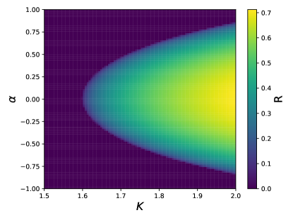
(a)

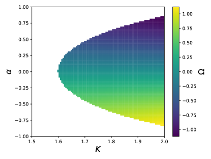
(b)

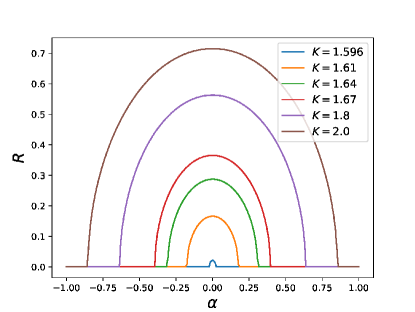
(c)

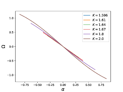
(d)

Figure 1: (a) Order-parameter diagram. (b) Synchronization-frequency diagram. (c) Graphs of $R$ for constant $K$ and varying $\alpha$. (d) Graphs of $\Omega$ for constant $K$ and varying $\alpha$. The values of $R$ and $\Omega$ are numerical approximations to solutions of the system of Eqs. (53-54). We assume that $g$ is a standard normal density.

Figure1(a) shows a $100\times 100$ resolution grid of points $(K,\alpha)$. Each point has a color defined according to the value of $R$, e.g. dark blue for $R=0$. A well-defined boundary separates two regions, one with $R=0$ and another where $R>0$. Figure 1(a) can be seen as a phase diagram pointing out the transition from a fully desynchronized state to a hybrid state consisting of both D and S oscillators.

Figure1(b) shows a similar grid to that of Fig.1(a). The grid has the same set of points $(K,\alpha)$, but the color of each point is defined by the corresponding value of $\Omega$. If $\Omega$ is not defined for a specific point, we associate this point with the white color.

In Figs. 1(c) and (d), we show slices of the three-dimensional graphs of Figs. 1(a) and (b). For each two-dimensional profile, $K$ is kept fixed, and $\alpha$ varies between $-1$ and $+1$. The graphs of Figure 1(c) suggest that, for constant $K$, $R$ is an even function of $\alpha$ with a maximum at $\alpha=0$. In Figure 1(d), the graphs indicate that $\Omega$ varies monotonically as an odd function of $\alpha$. Moreover, at least for the set of $K$ values considered, $\Omega$ is more sensitive to variations in $\alpha$ than in $K$.

3 Density of instantaneous frequencies

In the previous section, we showed how to obtain known results from the KS theory relevant to this work. We are now able to proceed towards our core result: the density of instantaneous frequencies in the KS model, which we represent by the probability density function $G$. The quantity $G(\nu)\,d\nu$ is then the probability that a KS oscillator $i$ has its fixed-frame instantaneous frequency, $\dot{\theta}_{i},$ in the interval $\left[\nu,\,\nu+d\nu\right)$.

In the process of obtaining $G$, we are concerned about the case $R>0$ (synchronization state). According to Eqs. (11) and (15), for $R=0$, $\dot{\theta}_{i}=\omega_{i}$. Then, in the incoherent state, the densities of instantaneous and natural frequencies are identical, i.e. $G(\nu)=g(\nu)$.

Before we show how to obtain the density $G$, we introduce some basic facts and definitions to simplify the notation. First, the product $KR$ is defined by

$$a\equiv KR,$$ (56)

and

$$\widetilde{x}\equiv\frac{x-\Omega}{a}$$ (57)

for a generic variable $x$. We can then rewrite Eqs. (22), (27), and (31) as

$$\psi^{*}(\omega)=\sin^{-1}\left(\widetilde{\omega}\right),$$ (58)

$$\dot{\psi}(\psi)=a\left(\widetilde{\omega}-\sin\psi\right),$$ (59)

and

$$C\left(\omega\right)=\frac{a}{2\pi}\operatorname{sgn}{\widetilde{\omega}}\sqrt{\widetilde{\omega}^{2}-1}.$$ (60)

In Eq. (60), $\operatorname{sgn}{\widetilde{\omega}}$ is the sign of $\widetilde{\omega}$ and $\left|\widetilde{\omega}\right|>1$. Another set of useful definitions is

$$\dot{\psi}\equiv\nu-\Omega,$$ (61)

$$\Delta\nu\equiv\widetilde{\nu}-\widetilde{\omega},$$ (62)

and the function

$$f_{\nu}(\psi)\equiv\Delta\nu+\sin(\psi).$$ (63)

The symbol $\dot{\psi}$ is used to denote the rotating-frame instantaneous frequency of an oscillator with a fixed-frame instantaneous frequency $\nu$. Definitions (61) and (62) imply

$$\widetilde{\nu}=\frac{\dot{\psi}}{a}$$ (64)

and

$$\Delta\nu=\frac{\dot{\psi}}{a}-\widetilde{\omega}.$$ (65)

From the formulas for $n_{S}(\psi|\omega)$ and $n_{D}(\psi|\omega)$, given by Eqs. (24) and (29), the phase density for an oscillator with known natural frequency $\omega$ is

$$n(\psi|\omega)=\begin{cases}\delta\left[\psi-\psi^{*}\left(\omega\right)\right],\quad&\left|\widetilde{\omega}\right|\leq 1\\ \\ \frac{C(\omega)}{\dot{\psi}(\psi)},&\left|\widetilde{\omega}\right|>1\end{cases}$$ (66)

where $\psi^{*}\left(\omega\right)$ and $C\left(\omega\right)$ is defined by Eqs. (58) and (60).

We now have enough mathematical tools to determine $G$. As a first step, we define $p(\dot{\psi}|\omega)$ as the probability density that an oscillator has a rotating-frame instantaneous frequency $\dot{\psi}$ given that the oscillator’s natural frequency is $\omega$. From the random variable transformation theorem [29], we have

$$p(\dot{\psi}|\omega)=\int_{-\pi}^{+\pi}\delta[\dot{\psi}-\dot{\psi}(\psi)]n(\psi|\omega)\,d\psi$$ (67)

In Eq. (67), $\dot{\psi}$ is the argument of function $p(\dot{\psi}|\omega)$, $\dot{\psi}(\psi)$ is the function of $\psi$ defined by Eq. (59), and $n(\psi|\omega)$ is the conditional density (66).

From Eqs. (66) and(67),

$$p(\dot{\psi}|\omega)=\begin{cases}p_{S}(\dot{\psi}|\omega),\quad&\left|\widetilde{\omega}\right|\leq 1\\ \\ p_{D}(\dot{\psi}|\omega),&\left|\widetilde{\omega}\right|>1\end{cases}$$ (68)

where

$$p_{S}(\dot{\psi}|\omega)=\frac{1}{a}\int_{-\pi}^{+\pi}\delta\left[\psi-\psi^{*}\left(\omega\right)\right]\delta\left[f_{\nu}(\psi)\right]\,d\psi$$ (69)

and

$$p_{D}(\dot{\psi}|\omega)=\frac{1}{2\pi a}\operatorname{sgn}{\widetilde{\omega}}\sqrt{\widetilde{\omega}^{2}-1}\int_{-\pi}^{+\pi}\frac{\delta\left[f_{\nu}(\psi)\right]}{\widetilde{\omega}-\sin\psi}\,d\psi.$$ (70)

By solving the integral in Eq. (69), we get $p_{S}(\dot{\psi}|\omega)=\delta\left\{af_{\nu}\left[\psi^{*}\left(\omega\right)\right]\right\}$. So, from (58), (61), (62), and (63),

$$p_{S}(\dot{\psi}|\omega)=\delta(\dot{\psi}),$$ (71)

which expresses the certainty that S oscillators have rotating-frame instantaneous frequencies equal to zero, i.e., their fixed-frame instantaneous frequencies are equal to $\Omega$.

To solve the integral in Eq. (70), we write $\delta\left[f_{\nu}(\psi)\right]$ as

$$\delta\left[f_{\nu}(\psi)\right]=\sum_{\beta\in O\left[f_{\nu}\right]}\frac{\delta(\psi-\beta)}{\left|f_{\nu}^{\prime}(\beta)\right|},$$ (72)

where $f_{\nu}^{\prime}$ is the derivative of $f_{\nu}$, and $\beta$ runs through $O\left[f_{\nu}\right]$, defined as the set of the simple zeros of $f_{\nu}$. If $O\left[f_{\nu}\right]$ is an empty set, which is the case for $\left|\Delta\nu\right|\geq 1$, $\delta\left[f_{\nu}(\psi)\right]=0$. For $\left|\Delta\nu\right|<1$, $f_{\nu}$ has two simple zeros: $\beta_{1}=\sin^{-1}\left(-\Delta\nu\right)$ and $\beta_{2}=\pi-\beta_{1}$. Since $\left|f_{\nu}^{\prime}\left(\beta_{1,2}\right)\right|=\left|\cos\left[\sin^{-1}\left(\Delta\nu\right)\right]\right|=\sqrt{1-\left(\Delta\nu\right)^{2}}$, Eq. (72) gives

$$\delta\left[f_{\nu}(\psi)\right]=\begin{cases}\frac{1}{\sqrt{1-\left(\Delta\nu\right)^{2}}}\left[\delta\left(\psi-\beta_{1}\right)+\delta\left(\psi-\beta_{2}\right)\right],\quad&\left|\Delta\nu\right|<1\\ \\ 0,&\left|\Delta\nu\right|\geq 1.\end{cases}$$ (73)

From Eqs. (70) and (73), we have

$$p_{D}(\dot{\psi}|\omega)=\begin{cases}\frac{\operatorname{sgn}{\widetilde{\omega}}}{\pi a\widetilde{\nu}}\sqrt{\frac{\widetilde{\omega}^{2}-1}{1-\left(\Delta\nu\right)^{2}}},\quad&\left|\Delta\nu\right|<1\\ \\ 0,&\left|\Delta\nu\right|\geq 1,\end{cases}$$ (74)

whose explicit dependence on $\dot{\psi}$ can be obtained using Eqs. (64) and (65).

With Eqs. (71) and (74), we complete the definition of the conditional density $p(\dot{\psi}|\omega)$, given by (68). In a similar way to what we have done to obtain the density of phases (See Eqs. (19), (20) and (21)), we can define the densities of instantaneous frequencies as

$$p(\dot{\psi})=p_{S}(\dot{\psi})+p_{D}(\dot{\psi}),$$ (75)

where

$$p_{S}(\dot{\psi})=\intop_{\left|\widetilde{\omega}\right|\leq 1}p_{S}(\dot{\psi}|\omega)g(\omega)\,d\omega$$ (76)

and

$$p_{D}(\dot{\psi})=\intop_{\left|\widetilde{\omega}\right|>1}p_{D}(\dot{\psi}|\omega)g(\omega)\,d\omega.$$ (77)

In Eqs. (76) and (77), $p_{S}(\dot{\psi})$ and $p_{D}(\dot{\psi})$ are the densities of instantaneous frequencies in the rotating frame for S and D oscillators, respectively.

Since the integration domain in (76) is the interval $\left[\Omega-a,\Omega+a\right]$, substituting (71) in (76) results in

$$p_{S}(\dot{\psi})=S(K,\alpha)\delta(\dot{\psi}),$$ (78)

where

$$S(K,\alpha)=\int_{\Omega-a}^{\Omega+a}g(\omega)d\omega.$$ (79)

The quantity $S(K,\alpha)$ has an important meaning: $S(K,\alpha)$ is the probability that an oscillator is synchronized. So, $S(K,\alpha)$ quantifies the fraction of S oscillators. Note that $S(K,\alpha)$ has implicit dependencies on $K$ and $\alpha$ through $\Omega$ and $a$. As already mentioned, $a=KR$, and the pair $\left\{\Omega,R\right\}$ is the solution of the system of Eqs. (53-54).

In order to obtain a formula for $p_{D}(\dot{\psi})$ from Eq. (77), it is useful to define $D(\nu)$ as the set of real numbers $\widetilde{\omega}$ such that $\left|\widetilde{\omega}\right|>1$ and $\left|\Delta\nu\right|<1$. That is,

$$D(\nu)\equiv\left\{\widetilde{\omega}\in{\rm I\!R}-\left[-1,+1\right]\mid\widetilde{\nu}-1<\widetilde{\omega}<\widetilde{\nu}+1\right\}.$$ (80)

Note that, for $\widetilde{\nu}=0$, $D(\nu)$ is the empty set. For finite $\widetilde{\nu}$, $D(\nu)$ is an open interval $\left(\widetilde{\omega}_{\nu}^{-},\widetilde{\omega}_{\nu}^{+}\right)$, whose endpoints $\widetilde{\omega}_{\nu}^{-}$ and $\widetilde{\omega}_{\nu}^{+}$ change according to the value of $\nu$. The endpoints of $D(\nu)$ are given in Table 1 for different intervals of $\tilde{\nu}$.

	$\tilde{\nu}\leq-2$	$-2<\tilde{\nu}<0$	$0<\tilde{\nu}<+2$	$+2\leq\tilde{\nu}$
$\widetilde{\omega}_{\nu}^{+}$	$\tilde{\nu}+1$	$-1$	$\tilde{\nu}+1$	$\tilde{\nu}+1$
$\widetilde{\omega}_{\nu}^{-}$	$\tilde{\nu}-1$	$\tilde{\nu}-1$	$+1$	$\tilde{\nu}-1$

Table 1: Endpoints of the open interval $D(\nu)=\left(\widetilde{\omega}_{\nu}^{-},\widetilde{\omega}_{\nu}^{+}\right)$, defined by (80). For $\widetilde{\nu}=0$, $D(\nu)$ is the empty set.

A more compact way of defining $\widetilde{\omega}_{\nu}^{-}$ and $\widetilde{\omega}_{\nu}^{+}$ is

$$\widetilde{\omega}_{\nu}^{\pm}=\left(\tilde{\nu}\pm 2\right)\Theta\left[\tilde{\nu}\left(\tilde{\nu}\pm 2\right)\right]\mp 1,$$ (81)

where $\Theta$ denotes the Heaviside step function with the standard definition $\Theta(0)=\frac{1}{2}$.

Let $\overline{D}(\nu)$ be the set of real numbers $\widetilde{\omega}$ such that $\left|\widetilde{\omega}\right|>1$ and $\left|\Delta\nu\right|\geq 1$. So, from (74) and (77),

$$p_{D}(\dot{\psi})=\int_{D(\nu)}p_{D}(\dot{\psi}|\omega)g(\omega)\,d\omega+\int_{\overline{D}(\nu)}p_{D}(\dot{\psi}|\omega)g(\omega)\,d\omega.$$ (82)

Since $p_{D}(\dot{\psi}|\omega)=0$ for $\left|\Delta\nu\right|\geq 1$ (See Eq. (74)), the second integral in (82) is zero. The first integral is also zero only if $D(\nu)$ is empty, that is, if $\widetilde{\nu}=0$ ($\dot{\psi}=0$). If $\widetilde{\nu}\neq 0$ ($\dot{\psi}\neq 0$), the first integral can be determined using the endpoints of $D(\nu)$ as integration limits and the expression of $p_{D}(\dot{\psi}|\omega)$ for $\left|\Delta\nu\right|<1$ defined in Eq. (74). Thus, Eq. (82) can be rewritten as

$$p_{D}(\dot{\psi})=\frac{a}{\pi\dot{\psi}}\int_{\widetilde{\omega}_{\dot{\psi}+\Omega}^{-}}^{\widetilde{\omega}_{\dot{\psi}+\Omega}^{+}}\operatorname{sgn}{\widetilde{\omega}}\sqrt{\frac{\widetilde{\omega}^{2}-1}{1-\left(\frac{\dot{\psi}}{a}-\widetilde{\omega}\right)^{2}}}g(a\widetilde{\omega}+\Omega)\,d\widetilde{\omega}$$ (83)

for non-zero values of $\dot{\psi}$, and $p_{D}(\dot{\psi})=0$ for $\dot{\psi}=0$. From (81), the limits of integration in (83) are

$$\widetilde{\omega}_{\dot{\psi}+\Omega}^{\pm}=\left(\frac{\dot{\psi}}{a}\pm 2\right)\Theta\left[\frac{\dot{\psi}}{a}\left(\frac{\dot{\psi}}{a}\pm 2\right)\right]\mp 1.$$ (84)

In order to show the explicit dependence of $p_{D}(\dot{\psi})$ on $\dot{\psi}$, we used (61), (64), and (65). We also changed the previous integration variable, $\omega$, to $\widetilde{\omega}$.

Equations (75), (78) and (83) give a full description of the density of instantaneous frequencies in the rotating frame. Our goal now is to obtain the density of fixed-frame instantaneous frequencies, which we defined, at the beginning of this section, as a probability density function $G(\nu).$

Instantaneous frequencies in the rotating and fixed frames are related through Eq. (61). Therefore, $G(\nu)=p(\nu-\Omega)$, which is the same as

$$G(\nu)=p_{S}(\nu-\Omega)+p_{D}(\nu-\Omega).$$ (85)

Let $G_{S}(\nu)=p_{S}(\nu-\Omega)$ and $G_{D}(\nu)=p_{D}(\nu-\Omega)$. From (78), (83), and (85), we have

$$G(\nu)=G_{S}(\nu)+G_{D}(\nu),$$ (86)

where

$$G_{S}(\nu)=S(K,\alpha)\delta(\nu-\Omega),$$ (87)

$$G_{D}(\nu)=\frac{1}{\pi\left|\widetilde{\nu}\right|}\int_{\widetilde{\omega}_{\nu}^{-}}^{\widetilde{\omega}_{\nu}^{+}}\sqrt{\frac{\widetilde{\omega}^{2}-1}{1-(\widetilde{\nu}-\widetilde{\omega})^{2}}}g(a\widetilde{\omega}+\Omega)\,d\widetilde{\omega},$$ (88)

for $\left|\nu-\Omega\right|>0$, and $G_{D}(\Omega)=0$. Note that we replaced $\frac{\operatorname{sgn}{\widetilde{\omega}}}{\widetilde{\nu}}$ with $\frac{1}{\left|\widetilde{\nu}\right|}$ to obtain Eq. (88). This is possible due to the integral-limits signs, which can be determined from Table 1. If $\widetilde{\nu}$ is positive, both $\widetilde{\omega}_{\nu}^{-}$ and $\widetilde{\omega}_{\nu}^{+}$ are positive. If $\widetilde{\nu}$ is negative, both $\widetilde{\omega}_{\nu}^{-}$ and $\widetilde{\omega}_{\nu}^{+}$ are negative. So, the integration variable, $\widetilde{\omega}$, which is in the interval $\widetilde{\omega}_{\nu}^{-}<\widetilde{\omega}<\widetilde{\omega}_{\nu}^{+}$, has the same sign as $\widetilde{\nu}$. This implies $\widetilde{\nu}=\operatorname{sgn}{\widetilde{\omega}}\left|\widetilde{\nu}\right|$.

An alternative formula for Eq. (88) can be obtained by changing the integration variable from $\widetilde{\omega}$ to $\psi=\sin^{-1}(\widetilde{\omega}-\widetilde{\nu})$. This change results in: $\widetilde{\omega}^{2}-1=(\sin\psi+\widetilde{\nu})^{2}-1$, $\sqrt{1-(\widetilde{\nu}-\widetilde{\omega})^{2}}=\cos\psi$, and $g(a\widetilde{\omega}+\Omega)=g(a\sin\psi+\nu)$. In addition, if $\psi_{\nu}^{-}$ and $\psi_{\nu}^{+}$ denote the new integral limits, then, from $\psi_{\nu}^{\pm}=\sin^{-1}(\widetilde{\omega}_{\nu}^{\pm}-\widetilde{\nu})$ and $\Theta(x)+\Theta(-x)=1$,

$$\psi_{\nu}^{\pm}=\sin^{-1}\left\{-\left(\tilde{\nu}\pm 2\right)\Theta\left[-\tilde{\nu}\left(\tilde{\nu}\pm 2\right)\right]\pm 1\right\}.$$ (89)

The formulas above allow us to rewrite Eq. (88) as

$$G_{D}(\nu)=\frac{1}{\pi\left|\widetilde{\nu}\right|}\int_{\psi_{\nu}^{-}}^{\psi_{\nu}^{+}}\sqrt{(\sin\psi+\widetilde{\nu})^{2}-1}g(a\sin\psi+\nu)\,d\psi.$$ (90)

Equations (86), (87), and (90) are identical to those which define the density of instantaneous frequencies in the Kuramoto model [26]. However, although the formulas in both models depend on $R$ and $\Omega$ in the same manner, $R$ and $\Omega$ depend implicitly on $\alpha$ in the KS model, while the parameter $\alpha$ is not defined in the Kuramoto model.

We conclude this section in a summary fashion presenting again our main result with the original notation restored and together with all auxiliary equations. From Eqs. (86), (87) and (88),

$$G(\nu)=S(K,\alpha)\delta(\nu-\Omega)+G_{D}(\nu),$$ (91)

where

$$S(K,\alpha)=\int_{\Omega-KR}^{\Omega+KR}g(\omega)d\omega,$$ (92)

and

$$G_{D}(\nu)=\frac{KR}{\pi\left[\left|\nu-\Omega\right|+\Theta(-\left|\nu-\Omega\right|)\right]}\int_{\widetilde{\omega}_{\nu}^{-}}^{\widetilde{\omega}_{\nu}^{+}}\sqrt{\frac{\widetilde{\omega}^{2}-1}{1-\left(\frac{\nu-\Omega}{KR}-\widetilde{\omega}\right)^{2}}}g(\Omega+KR\widetilde{\omega})\,d\widetilde{\omega},$$ (93)

which have the integral limits

$$\widetilde{\omega}_{\nu}^{\pm}=\left(\frac{\nu-\Omega}{KR}\pm 2\right)\Theta\left[\frac{\nu-\Omega}{KR}\left(\frac{\nu-\Omega}{KR}\pm 2\right)\right]\mp 1.$$ (94)

We introduced the function $\Theta(-\left|\nu-\Omega\right|)$ in (93) so that $G_{D}(\Omega)=0$, as stated earlier. The quantities $R$ and $\Omega$, which appear in Eqs. (91), (92), (93), and (94), form the solution of Eq. (37), namely

$$\frac{e^{i\alpha}}{K}=\intop_{-\frac{\pi}{2}}^{+\frac{\pi}{2}}e^{i\psi}g(\Omega+KR\sin\psi)\cos\psi\,d\psi+iJ,$$ (95)

where

$$J=\intop_{0}^{+\frac{\pi}{2}}\left\{g\left(\Omega+\frac{KR}{\sin\psi}\right)-g\left(\Omega-\frac{KR}{\sin\psi}\right)\right\}\frac{\cos\psi\left(1-\cos\psi\right)}{\sin^{3}\psi}\,d\psi.$$ (96)

Interestingly, from Eqs. (91) to (96), Eq. (95) is the only one in which the parameter $\alpha$ is present.

4 Application: Gaussian density of natural frequencies

In this section, we illustrate our analytical result assuming that natural frequencies are distributed according to the standard normal density (See Eq. (55)). Since a complete plot of $G$ cannot be drawn due to the delta term, we show in Figs. 2 and 3 only graphs of $S(K,\alpha)$ and $G_{D}$. The graphs come from Eqs. (92) and (93). Each graph consists of $250$ points.

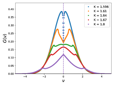
(a)

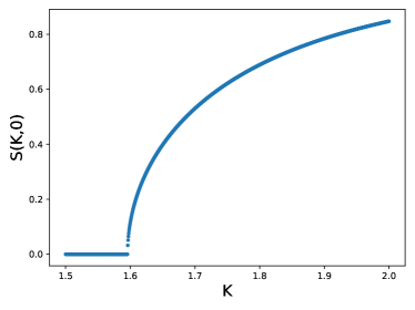
(b)

Figure 2: (a) Graphs of $G_{D}$ for $\alpha=0$. The dashed vertical line represents the delta term in (91). (b) Fraction of synchronized oscillators, $S(K,\alpha)$, for $\alpha=0$.

Fig. 2(a) shows graphs of $G_{D}$ with $\alpha=0$. This is the case for which the KS model reduces to the Kuramoto model. Each graph is plotted with $K$ fixed. The dashed vertical line points out the delta-term position, given by $\Omega=0$. The area below the curve connecting neighboring points of a graph of $G_{D}$ corresponds to the fraction of D oscillators. Fig. 2(a) indicates that the fraction of D oscillators diminishes as $K$ increases.

In Fig. 2(b), we show how $S(K,0)$, the fraction of S oscillators for $\alpha=0$, varies with $K$. For values of $K$ less than a critical value $K_{c}\simeq 1.5957$, $S(K,0)=0$, i.e. oscillators are all of D type. This is consistent with Fig. 1(a) and Eq. (92): for $K<K_{c}$ and $\alpha=0$, we have $R=0$, and then the integration range of Eq. (92) collapses, leading to $S(K,0)=0$. Note also that, in Fig. 2(a), for $K=1.596$, which is slightly greater than $K_{c}$, the graph of $G_{D}$ resembles, except near $\nu=0$, the profile of the standard normal density. As $K$ increases beyond $K_{c}$, Fig. 2(b) shows an increase of $S(K,0)$.

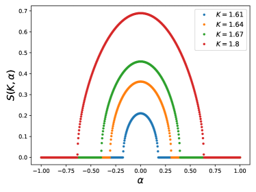
(a)

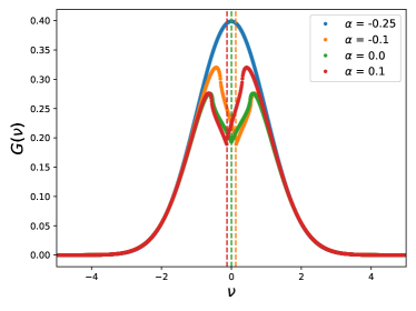
(b) $K=1.61$

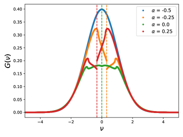
(c) $K=1.64$

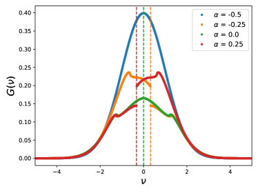
(d) $K=1.67$

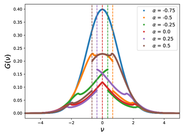
(e) $K=1.80$

Figure 3: (a) Fraction of synchronized oscillators, $S(K,\alpha)$. (b-e) Graphs of $g$ (in blue) and $G_{D}$. As in Fig. 2(a), the dashed vertical lines represent the delta term of $G$.

The plots in Figs. 3(a) show the effects of the parameter $\alpha$ on $S(K,\alpha)$. Each graph is plotted with $K$ fixed and $\alpha$ varying in the interval $[-1.0,+1.0]$. For higher values of $K$, $S(K,\alpha)$ has non-zero values over wider ranges of $\alpha$, and the maximum points of $S(K,\alpha)$ are positioned at higher levels. The graphs of $S(K,\alpha)$ are similar to those of $R$, shown in Fig. 1(c): if $R=0$, then $S(K,\alpha)=0$, as expected from Eq.(92); for $R>0$, the variation of $S(K,\alpha)$ follows closely that of $R$, suggesting a monotonic dependence of $S(K,\alpha)$ on $R.$

Graphs of $G_{D}$ and $g$ are shown in Figs. 3(b-e) for different values of $K$ and $\alpha$. Given $K$ and $\alpha$, if $R>0$, we show the corresponding $G_{D}$ graph and dashed line with the same color. If $R=0$ for a given pair $(K,\alpha)$, a graph of $g$, instead of a $G_{D}$ graph, is shown (with blue dots) to illustrate the profile of the instantaneous-frequency distribution in the incoherent state. The set of $K$ values used is the same as the one of Fig. 3(a).

Figures 3(b-e) show that, for $\alpha\neq 0$, $G_{D}$ has non-symmetric profiles. Yet, for $\alpha=0$, $G_{D}$ profiles are symmetric (See Fig. 2(a)). As discussed in Ref. [26], if $g$ has a profile with a symmetry axis (e.g. the standard normal density), $G_{D}$ profiles have the same symmetry axis in the Kuramoto model (KS model with $\alpha=0$). Another property of the graphs in Figs. 3(b-e) is that, for $\alpha\neq 0$, the dashed-line position also differs from zero. The dashed-line position, given by $\Omega$, has a sign opposite to the sign of $\alpha$, as shown in Fig. 1(d).

A remarkable feature of the graphs in Figs. 3(b-e) is the discontinuity at $\nu=\text{$\Omega$}$. For finite $\alpha$, the left and right non-symmetric branches of the graphs are visibly disconnected. For $\alpha=0$, the symmetric branches seem connected at $\nu=\Omega=0$, but, from Eq. (93), we know that $G_{D}(0)=0$, and the graphs indicate that $G_{D}(0^{+})=G_{D}(0^{-})>0$. Thus, a discontinuity seems to occur even in the symmetric profiles.

5 Numerical analysis

In Figs. 4 and 5, we show graphs of $G_{D}$ (in orange) and normalized histograms (in blue) of instantaneous frequencies obtained in numerical simulations of the KS model. By numerical simulation we mean numerical integration of the $N$ differential equations of the KS model from the initial time instant $0$ to a final one $T>0$. All simulations were performed with the numerical library ODEPACK [30]. The ODEPACK’s solver used is LSODA, a hybrid implementation of Adams and BDF methods [31]. Again, we assume a standard normal density of natural frequencies.

Before initiating a simulation, two random samples are generated: a sample $\left\{\omega_{i}\right\}_{i=1}^{N}$ of random natural frequencies and another one of random initial phases, $\left\{\theta_{i}(0)\right\}_{i=1}^{N}$. A standard-normal generator of random number s is used to create the sample of natural frequencies. The random initial phases are generated according to a uniform distribution in the interval $-\pi<\theta_{i}(0)<\pi$.

After a simulation is concluded, a normalized histogram (a histogram with the unit area) with bars of equal width is built from the instantaneous frequencies $\left\{\dot{\theta_{i}}(T)\right\}_{i=1}^{N}$, computed from Eqs. (1) and the numerically-obtained set of phases $\left\{\theta_{i}(T)\right\}_{i=1}^{N}$. For the histograms of Figs. 4 and 5, the simulation parameters are $N=5\times 10^{5}$ and $T=5\times 10^{2}$.

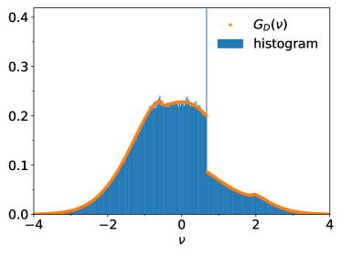
(a) $\alpha=-0.50$

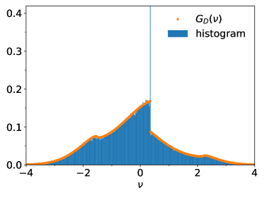
(b) $\alpha=-0.25$

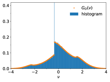
(c) $\alpha=+0.25$

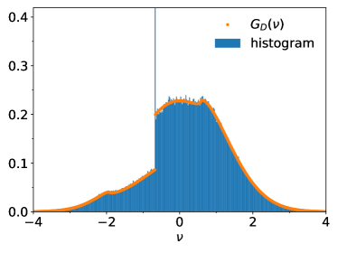
(d) $\alpha=+0.50$

Figure 4: In blue: normalized histograms of instantaneous frequencies obtained in numerical simulations of the Kuramoto-Sakaguchi model. In orange: graphs of $G_{D}$. For all simulations and graphs, $K=1.80$. Model size: $N=5\times 10^{5}$. Simulation time: $T=5\times 10^{2}$.

The occurrence of both S and D oscillators is depicted in the histograms of Figs. 4(a-d), where $K=1.80$, and $\alpha$ takes values in the set $\left\{-0.5,-0.25,+0.25,+0.5\right\}$. Figs. 4(a-d) show that the graphs of $G_{D}$ are in agreement with the histogram profiles. The histograms exhibit, at $\nu=\Omega$, tall and thin bars, which we refer to as peaks. The peaks are related to the delta term of the function $G$ (See Eq. (91)).

We avoided showing the peaks entirely because their height are much higher than the other histogram bars. The smaller the width of the peak, the higher its height. The peaks emerge due to the large accumulation of instantaneous frequencies, most of them from S oscillators. We draw the reader’s attention to the fact that the area of the peak is not exactly equal to $S(K,\alpha)$: a small part of the peak area contributes to the fraction of D oscillators, given by $1-S(K,\alpha)$. Yet, the peak area can be a good approximation to $S(K,\alpha)$, depending on how small is the peak width.

A noteworthy property is the seeming reflection symmetry around the peaks. The reflection symmetry is related to sign inversions in the parameter $\alpha$: if the signal of $\alpha$ is inverted, keeping fixed its absolute value, the right (or left) side of the graphs and histograms are reflected on the left (or right) side.

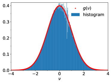
(a) $K=1.67$; $\alpha=-0.50$

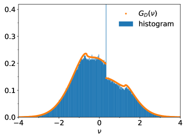
(b) $K=1.67$; $\alpha=-0.25$

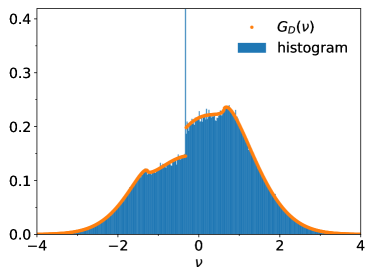
(c) $K=1.67$; $\alpha=+0.25$

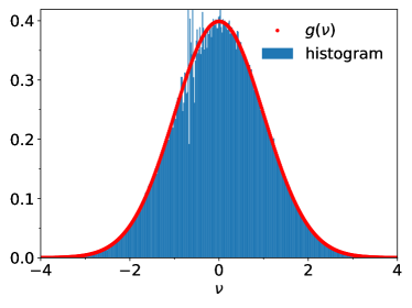
(d) $K=1.67$; $\alpha=+0.50$

Figure 5: In blue: normalized histograms of instantaneous frequencies obtained numerically. In red: graphs of $g$ (a,d). In orange: graphs of $G_{D}$ (b,c). The values of $\alpha$ are the same as in Fig. 4. In all simulations and graphs, $K=1.67$. Model size: $N=5\times 10^{5}$. Simulation time: $T=5\times 10^{2}$.

The same type of symmetry is observed in Figs. 5(a-d), where $K=1.60$, and the set of $\alpha$ values is the same as in Figs. 4(a-d). In Figs. 5(a) and 5(d) we plot $g$ (in red) instead of $G_{D},$ since $R=0$ (incoherent state) for the values of $K$ and $\alpha$ considered (as indicated in Fig. 1(c)). The curves of $g$ fit histograms showing no clearly visible peaks. A synchronization state is represented in Figs. 5(b) and 5(c). The curves of $G_{D}$ (in orange) also fit the histograms, but small deviations occur due to time fluctuations in the histogram bars.

Such fluctuations and deviations are also present in the histograms of Figs. 6(a-c). The deviations occur near the synchronization peak. The sequence of figures 6(a), 6(b) and 6(c) depicts the evolution of the instantaneous-frequency distribution in histograms from three different time instants of the same simulation: $T_{1}=500$, $T_{2}=1000$, and $T_{3}=1500$. The simulation time interval is $\left[0,T_{3}\right]$, and we define $K=1.64$, $\alpha=0.25$, and $N=5\times 10^{5}$. Again, initial phases and natural frequencies are random numbers generated according to the uniform and standard normal distributions.

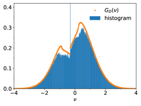
(a) $N=5\times 10^{5}$; $T_{1}=500$

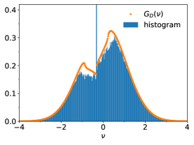
(b) $N=5\times 10^{5}$; $T_{2}=1000$

(c) $N=5\times 10^{5}$; $T_{3}=1500$

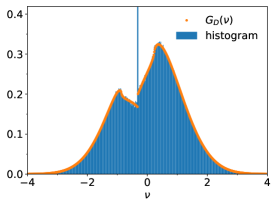
(d) $N=1.5\times 10^{6}$; $T_{1}=500$

(e) $N=1.5\times 10^{6}$; $T_{2}=1000$

(f) $N=1.5\times 10^{6}$; $T_{3}=1500$

Figure 6: In blue: normalized histograms of instantaneous frequencies at the time instants $T_{1}$, $T_{2},$ and $T_{3}$ obtained in two simulations of the KS model performed in the time interval $\left[0,T_{3}\right]$ and with different numbers of oscillators: one with $N=5\times 10^{5}$ and the other with $N=1.5\times 10^{6}$. The histograms in (a), (b) and (c) result from the simulation with the smallest $N$, while those in (d), (e), and (f), from the one with the highest $N$. For all simulations and graphs of $G_{D}$ (in orange), $K=1.64$ and $\alpha=0.25$.

The histograms of Figs .6(d), 6(e), and 6(f) comes from a simulation similar to the previous one. The difference is that the number of oscillators is three times higher, requiring a new random sample of initial phases and natural frequencies. The histograms show a more stationary profile in the sequence of time instants $T_{1}$, $T_{2},$ and $T_{3}$. In addition, the graphs of $G_{D}$ are in better agreement with the histogram profiles.

6 Conclusions

In this work, we showed how to obtain the density of instantaneous frequencies in the Kuramoto-Sakaguchi model. The density of instantaneous frequencies is a stationary probability density function with a complex formula given by the sum of two terms: a Dirac-delta-type function and a discontinuous one.

The Dirac-delta term is located in the synchronization frequency and carries information about the number of synchronized oscillators. The other term is discontinuous at a point defined also by the synchronization-frequency value. The discontinuous term have profiles with varied and unexpected shapes, and the area below them gives the fraction of out-of-synchrony oscillators.

Our formula is a generalization of the one obtained in Ref. [26] for the Kuramoto model (i.e. Kuramoto-Sakaguchi model with a phase-lag equal to zero). The formulas are mathematically quite similar, particularly concerning the property that the generalization has no explicit dependence on the phase-lag parameter. Indeed, the dependence on the phase-lag is implicit and takes place through the order parameter and the synchronization frequency.

Contrary to what was shown for the Kuramoto model in Ref. [26], natural-frequency densities with a symmetry axis in the synchronization frequency does not imply the same type of symmetry in the density of instantaneous frequencies for the Kuramoto-Sakaguchi model. However, this density exhibits a reflection symmetry, characterized by a flip of the density profile induced by sign inversions in the phase-lag parameter.

Our result is in accordance with numerical simulations of the Kuramoto-Sakaguchi model, provided simulations are performed with a large enough number of oscillators. If the number of oscillators is such that the instantaneous-frequency distribution from simulations (normalized histograms) shows significant non-stationary behavior, one observes a less robust fit to simulation data. But increasing the number of oscillators suppresses the non-stationarity and improves the quality of the theoretical prediction. These finite-size effects, also analyzed in the context of the Kuramoto model [26], are expected to occur in the Kuramoto-Sakaguchi model. Our result is based on the Kuramoto-Sakaguchi theory, which includes equilibrium assumptions devised under the requirement of an infinite number of oscillators and infinitely long times.

New research directions can be taken with this work as a starting point. A mathematically-oriented subject would be finding asymptotic analytical properties of the density function near the synchronization frequency as well as in its tails. Extending the study presented here, considering other types of natural-frequency densities, including non-symmetric and non-unimodal ones, is also an interesting topic. In addition, our formula can be used to determine the instantaneous-frequency statistical moments, which can then be compared to the moments of the natural frequencies and used to compute relevant quantities such as expected values and variances.

More importantly, we envision a non-stationary model capturing the collective dynamics of the instantaneous frequencies. We conjecture that the model solution would be a time-dependent density of instantaneous frequencies, and our formula would reflect the solution behavior in the long-time limit.

References

- [1] A. Pikovsky, M. Rosenblum, and J. Kurths, Synchronization, A Universal Concept in Nonlinear Sciences (Cambridge University Press, Cambridge, 2001).
- [2] A. E. Motter, S. A. Myers, M. Anghel, and T. Nishikawa, Nat. Phys. 9, 191 (2013).
- [3] G. Kozyreff, A. G. Vladimirov, and P. Mandel, Phys. Rev. Lett. 85, 3809 (2000).
- [4] A. T. Winfree, The Geometry of Biological Times (Springer, New York, 1980).
- [5] M. Breakspear, S. Heitmann, and A. Daffertshofer, Front. Human Neurosci. 4, 190 (2010).
- [6] A. T. Winfree, J. Theor. Biol. 16, 15 (1967).
- [7] Y. Kuramoto, International Symposium on Mathematical Problems in Theoretical Physics, edited by H. Araki, Lecture Notes in Physics No. 30 (Springer, New York, p. 420).
- [8] Y. Kuramoto, Chemical Oscillations, Waves and Turbulence (Springer-Verlag, Berlin, 1984).
- [9] Video message from Yoshiki Kuramoto to the international conference “Dynamics of Coupled Oscillators: 40 Years of the Kuramoto Model” https://youtu.be/lac4TxWyBOg
- [10] S.H. Strogatz, Physica D 143, 1 (2000).
- [11] J. D. da Fonseca, and C.V. Abud, Journal of Statistical Mechanics: Theory and Experiment, 103204 (2018).
- [12] J. A. Acebrón, L. L. Bonilla, C. J. P. Vicente, F. Ritort, and R. Spigler, Rev. Mod. Phys. 77, 137 (2005).
- [13] S. Gupta, A. Campa, and S. Ruffo, J. Stat. Mech. Theory Exp., 2014, R08001.
- [14] F. A. Rodrigues, T. K. D. Peron, P. Ji, and J. Kurths, Phys. Rep. 610, 1 (2016).
- [15] A. Mihara, E. S. Medeiros, A. Zakharova, and R. O. Medrano-T, Chaos 32, 033114 (2022).
- [16] A. Mihara, and R. O. Medrano-T, Nonlinear Dyn. 98, 539, (2019).
- [17] D. A. Wiley, S. H. Strogatz, and M. Girvan, Chaos 16, 015103 (2016).
- [18] A. Mihara, M. Zaks, E. E. N. Macau, and R. O. Medrano-T, Phys. Rev. E 105, L052202 (2022).
- [19] H. Sakaguchi and Y. Kuramoto, Progr. Theoret. Phys. 76, 576 (1986) .
- [20] D. M. Abrams, R. Mirollo, S. H. Strogatz, and D. A. Wiley, Phys. Rev. Lett. 101, 084103 (2008).
- [21] C. R. Laing, Chaos 19, 013113 (2009).
- [22] M. Wolfrum, and O. E. Omel’chenko, Phys. Rev. E 84, 015201 (2011).
- [23] D. Pazó, and E. Montbrió, Phys. Rev. X 4, 011009 (2014).
- [24] K. Wiesenfeld, P. Colet, and S.H. Strogatz, Phys. Rev. Lett. 76, 404 (1996).
- [25] S. M. Crook, G. B. Ermentrout, M. C. Vanier, and J. M. Bower, J. Comput. Neurosci. 4, 161 (1997).
- [26] J. D. da Fonseca, E. D. Leonel, and H. Chaté, Phys. Rev. E 102, 052127 (2020).
- [27] S. Gradshteyn, and I. M. Ryzhik, Table of Integrals, Series, and Products (Academic, New York, 2007)
- [28] J. J. Moré, B. S. Garbow, and K. E. Hillstrom, User Guide for MINPACK-1, Argonne National Laboratory Report ANL-80-74, Argonne, Ill., 1980.
- [29] D. T. Gillepsie, American Journal of Physics 51, 520 (1983).
- [30] A. C. Hindmarsh, “ODEPACK, A Systematized Collection of ODE Solvers,” IMACS Transactions on Scientific Computation, Vol 1., pp. 55-64, 1983.
- [31] L. Petzold, SIAM Journal on Scientific and Statistical Computing, Vol. 4, No. 1, pp. 136-148, 1983.
- [32] B. Ottino-Löffler and S. H. Strogatz, Chaos 26, 094804 (2016).