Continual Learning with Evolving Class Ontologies

Abstract

Lifelong learners must recognize concept vocabularies that evolve over time. A common yet underexplored scenario is learning with class labels that continually refine/expand old classes. For example, humans learn to recognize dog before dog breeds. In practical settings, dataset versioning often introduces refinement to ontologies, such as autonomous vehicle benchmarks that refine a previous vehicle class into school-bus as autonomous operations expand to new cities. This paper formalizes a protocol for studying the problem of Learning with Evolving Class Ontology (LECO). LECO requires learning classifiers in distinct time periods (TPs); each TP introduces a new ontology of “fine” labels that refines old ontologies of “coarse” labels (e.g., dog breeds that refine the previous dog). LECO explores such questions as whether to annotate new data or relabel the old, how to exploit coarse labels, and whether to finetune the previous TP’s model or train from scratch. To answer these questions, we leverage insights from related problems such as class-incremental learning. We validate them under the LECO protocol through the lens of image classification (on CIFAR and iNaturalist) and semantic segmentation (on Mapillary). Extensive experiments lead to some surprising conclusions; while the current status quo in the field is to relabel existing datasets with new class ontologies (such as COCO-to-LVIS or Mapillary1.2-to-2.0), LECO demonstrates that a far better strategy is to annotate new data with the new ontology. However, this produces an aggregate dataset with inconsistent old-vs-new labels, complicating learning. To address this challenge, we adopt methods from semi-supervised and partial-label learning. We demonstrate that such strategies can surprisingly be made near-optimal, in the sense of approaching an “oracle” that learns on the aggregate dataset exhaustively labeled with the newest ontology.

1 Introduction

Humans, as lifelong learners, learn to recognize the ontology of concepts which is being refined and expanded over time. For example, we learn to recognize dog and then dog breeds (refining the class dog). The class ontology often evolves from coarse to fine concepts in the real open world and can sometimes introduce new classes. We call this Learning with Evolving Class Ontology (LECO).

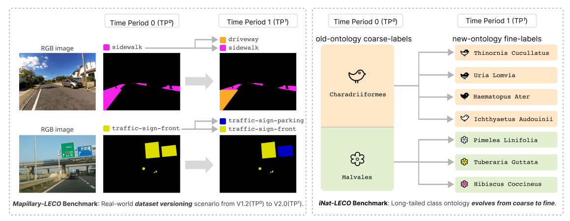
Figure 1: Learning with Evolving Class Ontology (LECO) requires training models in time periods (TPs) with new ontologies that refine/expand the previous ones. Left: The Mapillary dataset, which was constructed to study semantic segmentation for autonomous vehicles, has updated versions from V1.2 [55] to V2.0 [52], which refined previous labels with fine-grained ones on the same data, e.g., V1.2’s sidewalk is split to V2.0’s sidewalk and driveway. The visual demonstration with semantic segmentation ground-truth blacks out unrelated classes for clarity. We explore LECO using this dataset. Right: To study LECO, we also repurpose the large-scale iNaturalist dataset [75, 69, 33, 34, 35, 36, 37] to simulate the coarse-to-fine ontology evolution through the lens of image classification. LECO asks the first basic question: for the new TP that defines new ontology of classes, should one relabel the old data or label new data? Interestingly, both labeling protocols have been used in the community for large-scale datasets. Our study provides the (perhaps obvious) answer – one should always annotate new data with the new ontology rather than re-annotating the old. One reason is that the former produces more labeled data. But this produces an aggregate dataset with inconsistent old-vs-new labels. We make use of insights from semi-supervised learning and learning-with-partial-labels to learn from such heterogenous annotations, approaching the upper bound of learning from an oracle aggregate dataset with all new labels.

Motivation. LECO is common when building machine-learning systems in practice. One often trains and maintains machine-learned models with class labels (or a class ontology) that are refined over time periods (TPs) (Fig. 2). Such ontology evolution can be caused by new requirements in applications, such as autonomous vehicles that expand operations to new cities. This is well demonstrated in many contemporary large-scale datasets that release updated versions by refining and expanding classes, such as Mapillary [55, 52], Argoverse [12, 78], KITTI [23, 4] and iNaturalist [75, 69, 33, 34, 35, 36, 37]. For example, Mapillary V1.2 [55] defined the road class, and Mapillary V2.0 [52] refined it with fine labels including parking-aisle and road-shoulder; Argoverse V1.0 [12] defined the bus class, and Argoverse V2.0 [78] refined it with fine classes including school-bus.

Prior art. LECO requires learning new classes continually in TPs, similar to class-incremental learning (CIL) [47, 74, 86, 18]. They differ in important ways. First, CIL assumes brand-new labels that have no relations with the old [60, 47, 49], while LECO’s new labels are fine-grained ones that expand the old / “coarse” labels (cf. Fig. 2). Interestingly, CIL can be seen as a special case of LECO by making use of a “catch-all” background class [41] (often denoted as void or unlabeled in existing datasets [22, 14, 55, 52, 49]), which can be refined over time to include specific classes that were previously ignored. Second, CIL restricts itself to a small memory buffer for storing historical data to focus on information retention and catastrophic forgetting [47, 10]. However, LECO stores all historical data (since large-scale human annotations typically come at a much higher cost than that of the additional storage) and is concerned with the most-recent classes of interest. Most related to LECO are approaches that explore the relationship of new classes to old ones; Sariyildiz et al. [64] study concept similarity but remove common superclasses in their study, while Abdelsalam et al. [1] explore CIL with a goal to discover inter-class relations on data labeled (as opposed to assuming such relationships can be derived from a given taxonomic hierarchy). To explore LECO, we set up its benchmarking protocol (Section 3) and study extensive methods modified from those of related problems (Sections 4, 5, and 6).

Technical insights. LECO studies learning strategies and answers questions as basic as whether one should label new data or relabel the old data. Interestingly, both protocols have been used in the community for large-scale dataset versioning: Argoverse [12, 78] annotates new data, while Mapillary [55, 52] relabels its old data. Our experiments provide a definitive answer – one should always annotate new data with the new ontology rather than reannotating the old data. The simple reason is that the former produces more labeled data. However, this comes at a cost: the aggregate dataset is now labeled with inconsistent old-vs-new annotations, complicating learning. We show that joint-training [47] on both new and old ontologies, when combined with semi-supervised learning (SSL), can be remarkably effective. Concretely, we generate pseudo labels for the new ontology on the old data. But because pseudo labels are noisy [44, 79, 68, 58] and potentially biased [77], we make use of the coarse labels from the old-ontology as “coarse supervision”, or the coarse-fine label relationships [26, 61, 73, 45], to reconcile conflicts between the pseudo fine labels and the true coarse labels (Section 6). There is another natural question: should one finetune the previous TP’s model or train from scratch? One may think the former has no benefit (because it accesses the same training data) and might suffer from local minima. Suprisingly, we find finetuning actually works much better, echoing curriculum learning [21, 63, 5]. Perhaps most suprisingly, we demonstrate that such strategies are near optimal, approaching an “upperbound” that trains on all available data re-annotated with the new ontology.

Salient results. To study LECO, we repurpose three datasets: CIFAR100, iNaturlist, and Mapillary (Table 1). The latter two large-scale datasets have long-tailed distribution of class labels; particularly, Mapillary’s new ontology does not have strictly surjective mapping to the old, because it relabeled the same data from scratch with new ontology. Our results on these datasets lead to consistent technical insights summarized above. We preview the results on the iNaturalist-LECO setup (which simulates the large-scale long-tailed scenario): (1) finetuning the previous TP’s model outperforms training from scratch on data labeled with new ontology: 73.64% vs. 65.40% in accuracy; (2) jointly training on both old and new data significantly boosts accuracy to 82.98%; (3) taking advantage of the relationship between old and new labels (via Learning-with-Partial-Labels and SSL with pseudo-label refinement) further improves to 84.34%, effectively reaching an “upperbound” 84.51%!

Contributions. We make three major contributions. First, we motivate the problem LECO and define its benchmarking protocol. Second, we extensively study approaches to LECO by modifying methods from related problems, including semi-supervised learning, class-incremental learning, and learning with partial labels. Third, we draw consistent conclusions and technical insights, as described above.

2 Related Work

Class-incremental learning (CIL) [47, 74, 86, 18] and LECO both require learning classifiers for new classes over distinct time periods (TPs), but they have important differences. First, the typical CIL setup assumes new labels have no relations with the old [47, 49, 1], while LECO’s new labels refine or expand the old / “coarse” labels (cf. Fig. 2). Second, CIL purposely sets a small memory buffer (for storing labeled data) and evaluates accuracy over both old and new classes with the emphasis on information retention or catastrophic forgetting [40, 83, 47, 10]. However, LECO allows all (history) labeled data to be stored and highlight the difficulty of learning new classes which are fine/subclasses of the old ones. Further, we note that many real-world applications store history data (and should not limit a buffer size to save data) for privacy-related consideration (e.g., medical data records) and as forensic evidence (e.g., videos from surveillance cameras). Therefore, to approach LECO, we apply CIL methods that do not restrict buffer size, which usually serve as upper bounds in CIL [17]. In this work, we repurpose “upper bound” CIL methods for LECO including finetuning [80, 3], joint training [11, 47, 50, 51], as well as the “lower bound” methods by freezing the backbone [20, 66, 3].

Semi-supervised learning (SSL) learns over both labeled and unlabeled data. State-of-the-art SSL methods follow a self-training paradigm [65, 54, 79] that uses a model trained over labeled data to pseudo-label the unlabeled samples, which are then used together with labeled data for training. For example, Lee et al. [44] use confident predictions as target labels for unlabeled data, and Rizve et al. [62] further incorporate low-probability predictions as negative pseudo labels. Some others improve SSL using self-supervised learning techniques [24, 84], which force predictions to be similar for different augmentations of the same data [6, 7, 68, 79, 85]. We leverage insights of SSL to approach LECO, e.g., pseudo labeling the old data. As pseudo labels are often biased [77], we further exploit the old-ontology to reject or improve the inconsistent pseudo labels, yielding better performance.

Benchmark	#TPs	#classes/TP	#train/TP	#test/TP
CIFAR-LECO	2	20/100	10k	10k
iNat-LECO	2	123/810	50k	4k
Mapillary-LECO	2	66/116	2.5k	2k
iNat-4TP-LECO	4	123/339/729/810	25k	4k

Table 1: LECO benchmarks use CIFAR100 [42], iNaturalist [75, 69], and Mapillary [55, 52]. We also vary the number of training data in experiments; as conclusions hold across settings, we report these results in Table 9, 10, 11.

Learning with partial labels (LPL) tackles the case when some examples are fully labeled while others are only partially labeled [26, 56, 53, 15, 9, 88]. In the area of fine-grained recognition, partial labels can be coarse superclasses which annotate some training data [61, 45, 73, 31]. In a TP of LECO, the old data from previous TPs can be used as partially-labeled examples as they contain only coarse labels. Therefore, to approach LECO, we explore state-of-the-art methods [70] in this line of work. However, it is important to note that ontology evolution in LECO can be more than splitting old classes, e.g., the new class special-subject can be a result of merging multiple classes child and police-officer. Indeed, we find it happens quite often in the ontology evolution from the Mapillary’s versioning from V1.2 [55] to V2.0 [52]. In this case, the LPL method does not show better results than the simple joint training approach (31.04 vs. 31.05 on Mapillary in Table 4).

3 Problem Setup of Learning with Evolving Class Ontology (LECO)

Notations. Among $T$ time periods (TPs), TP^t has data distributions $\mathcal{D}^{t}=\mathbf{X}\times\mathbf{Y}^{t}$, where $\mathbf{X}$ is the input and $\mathbf{Y}^{t}$ is the label set. The evolution of class ontology is ideally modeled as a tree structure: the $i^{th}$ class $\mathbf{y}^{t}_{i}\in\mathbf{Y}^{t}$ is a node that has a unique parent ${\bf y}^{t-1}_{j}\in\mathbf{Y}^{t-1}$, which can be split into multiple fine classes in TP^t. Therefore, $|{\bf Y}^{t}|>|{\bf Y}^{t-1}|$. TP^t concerns classification w.r.t label set ${\bf Y}^{t}$.

Benchmarks. We define LECO benchmarks using three datasets: CIFAR100 [42], iNaturalist [75, 69], and Mapillary [52, 55] (Table 1). CIFAR100 is released under the MIT license, and iNaturalist and Mapillary are publicly available for non-commercial research and educational purposes. CIFAR100 and Mapillary contain classes related to person and potentially have fairness and privacy concerns, hence we cautiously proceed our research and release our code under the MIT License without re-distributing the data. The iNaturalist and Mapillary are large-scale and have long-tailed class distributions (refer to the Table 4 and 5 for class distributions). For each benchmark, we sample data from the corresponding dataset to construct time periods (TPs), e.g., TP⁰ and TP¹ define their own ontologies of class labels ${\bf Y}^{0}$ and ${\bf Y}^{1}$, respectively. For CIFAR-LECO, we use the two-level hierarchy offered by the original CIFAR100 dataset [42]: using the 20 superclasses as the ontology in TP⁰, each of them is split into 5 subclasses as new ontology in TP¹. For iNat-LECO, we used the most recent version of Semi-iNat-2021 [71] that comes with rich taxonomic labels at seven-level hierarchy. To construct two TPs, we choose the third level (i.e., “order”) with 123 categories for TP⁰, and the seventh (“species”) with 810 categories for TP¹. We further construct four TPs with each having an ontology out of four at distinct taxa levels [“order”, “family”, “genus”, “species”]. For Mapillary-LECO, we use its ontology of V1.2 [55] (2017) in TP⁰, and that of V2.0 [52] (2021) in TP¹. It is worth noting that, as a real-world LECO example, Mapillary includes a catch-all background class (aka void) in V1.2, which was split into meaningful fine classes in V2.0, such as temporary-barrier, traffic-island and void-ground.

Moreover, in each TP of benchmark CIFAR-LECO and iNat-LECO, we randomly sample 20% data as validation set for hyperparameter tuning and model select. We use their official valsets as our test-sets for benchmarking. In Mapillary-LECO, we do not use a valset but instead use the default hyperparameters reported in [72], tuned to optimize another related dataset Cityscapes [14]. We find it unreasonably computational demanding to tune on large-scale semantic segmentation datasets. Table 1 summarizes our benchmarks’ statistics.

Remark: beyond class refining in ontology evolution. In practice, ontology evolution also contains the case of class merging, as well as class renaming (which is trivial to address). The Mapillary’s versioning clearly demonstrates this: 10 of 66 classes of its V1.2 were refined into new classes, resulting into 116 classes in total of its V2.0; objects of the same old class were either merged into a new class or assigned with new fine classes. Because of these non-trivial cases under the Mapillary-LECO benchmark, state-of-the-art methods of learning with partial labels are less effective but our other solutions work well.

Remark: number of TPs and buffer size. For most experiments, we set two TPs. One may think more TPs are required for experiments because CIL literature does so [47, 74, 86, 18]. Recall that CIL emphasizes catastrophic forgetting issue caused by using limited buffer to save history data, so using more TPs for more classes and limited buffer helps exacerbate this issue. Differently, LECO emphasizes the difficulty of learning new classes that are subclasses of the old ones, and does not limit a buffer to store history data. Therefore, using two TPs are sufficient to show the difficulty. Even so, we have experiments that set four TPs, which demosntrate consistent conclusions drawn from those using two TPs. Moreover, even with unlimited buffer, CIL methods still work poorly on LECO benchmarks (cf. “TrainScratch” [59] and “FreezePrev” [47] in Table 2).

Metric. Our benchmarks study LECO through the lens of image classification (on CIFAR-LECO and iNat-LECO) and semantic segmentation (on Mapillary-LECO). Therefore, we evaluate methods using mean accuracy (mAcc) averaged over per-class accuracies, and mean intersection-over-union (mIoU) averaged over classes, respectively. The metrics treat all classes equally, avoiding the bias towards common classes due to the natural long-tailed class distribution (cf. iNaturalist [75, 69] and Mapillary [55]) (cf. class distributions in the appendix). We do not use specific algorithms to address the long-tailed recognition problem but instead adopt the recent simple technique to improve performance by tuning weight decay [2]. We run each method five times using random seeds on CIFAR-LECO and iNat-LECO, and report their averaged mAcc with standard deviations. For Mapillary, due to exoribitant training cost, we perform one run to benchmark methods.

4 Baseline Approaches to LECO

We first repurpose CIL and continual learning methods as baselines to approach LECO, as both require learning classifiers for new classes in TPs. We start with preliminary backgrounds.

Preliminaries. Following prior art [47, 39], we train convolutional neural networks (CNNs) and treat a network as a feature extractor $f$ (parametrized by $\theta_{f}$) plus a classifier $g$ (parameterized by $\theta_{g}$). The feature extractor $f$ consists of all the layers below the penultimate layer of ResNet [28], and the classifier $g$ is the linear classifier followed by softmax normalization. Specifically, in TP^t, an input image $x$ is fed into $f$ to obtain its feature representation $z=f(x;\theta_{f})$. The feature $z$ is then fed into $g$ for the softmax probabilities, $q=g(z;\theta_{g})$, w.r.t classes in ${\bf Y}^{t}$. We train CNNs by minimizing the Cross Entropy (CE) loss using mini-batch SGD. At TP^t, to construct a training batch $\mathcal{B}^{t}$, we randomly sample $K$ examples, i.e., $\mathcal{B}^{t}=\{(x_{1},y_{1}^{t}),\cdots,(x_{K},y_{K}^{t})\}$. The CE loss on $\mathcal{B}^{t}$ is

$$\small\mathcal{L}(\mathcal{B}^{t})=-\sum_{(x_{k},y_{k}^{t})\in\mathcal{B}^{t}}\mathcal{H}(y_{k}^{t},g(f(x_{k})))$$ (1)

where $\mathcal{H}(p,q)=-\sum_{c}p(c)log(q(c))$ is the entropy between two probability vectors.

Similary, for semantic segmentation, we use the same CE loss 1 at pixel level, along with the recent architecture HRNet with OCR module [72, 76, 81] (refer to appendix C for details).

Annotation Strategies. Closely related to LECO is the problem of class-incremental learning (CIL) or more generally, continual learning (CL) [60, 47, 86, 59, 83]. However, unlike typical CL benchmarks, LECO does not artificially limit the buffer size for storing history samples. Indeed, the expense of hard drive buffer is less of a problem compared to the high cost of data annotation. Therefore, LECO embraces all the history labeled data, regardless of being annoated using old or new ontologies. This leads to a fundamental question: whether to annotate new data or re-label the old, given a fixed labeling budget $N$ at each TP (cf. Fig. 2)?

• (LabelNew) Sample and annotate $N$ new examples using new ontology, which trivially infers the old-ontology labels. We further have the history data as labeled with old ontology.

• (RelabelOld) Re-annotate the $N$ history data using new ontology. However, these $N$ examples are all available data although they have both old- and new-ontology labels.

The answer is perhaps obvious – LabelNew – because it produces more labeled data. Furthermore, LabelNew allows one to exploit the old data to boost performance (Section 5). With proper techniques, this significantly reduces the performance gap with a model trained over both old and new data assumably annotated with new-ontology, termed as AllFine short for “supervised learning with all fine labels”.

Training Strategies. We consider CL baseline methods as LECO baselines. When new tasks (i.e., classes of ${\bf Y}^{t}$) arrive in TP^t, it is desirable to transfer model weights trained for ${\bf Y}^{t-1}$ in TP^t-1 [47, 60]. To do so, we initialize weights $\theta_{f^{t}}$ of the feature extractor $f^{t}$ with $\theta_{f^{t-1}}$ trained in TP^t-1, i.e., $\theta_{f^{t}}\coloneqq\theta_{f^{t-1}}$. Then we can

• (FreezePrev) Freeze $f^{t}$ to extract features, and learn a classifier $g^{t}$ over them [47].

• (FinetunePrev) Finetune $f^{t}$ and learn a classifier $g^{t}$ altogether [47].

• (TrainScratch) Train $f^{t}$ from random weights [59].

Table 2: Results of baseline methods for LECO (more results in the Table 9). For all our experiments, we run each method five times and report the averaged mean per-class accuracy/intersection-over-union (mAcc/mIoU in $\%$) with standard deviations when available. For each benchmark, we bold the best mAcc/mIoU including ties that fall within its std. FinetunePrev is the best learning strategy that outperforms TrainScratch (cf. 73.64% vs. 65.69% with LabelNew on iNat-LECO). This implies that the coarse-to-fine evolved ontology serves as a good learning curriculum. FreezePrev underperforms TrainScratch (cf. 50.82% vs. 65.69% with LabelNew on iNat-LECO), confirming the difficulty of learning new classes that refine the old. LabelNew and RelabelOld achieve similar performance with the former using only new data but not the old altogether. If using both old and new data, we boost performance as shown in Table 3. The conclusions hold for varied number of training images and generalize to the Mapillary experiments, yet all methods fall short to the AllFine (which trains on all data assumed to be labeled with new ontology).

Benchmark	$\#$images / TP	TP0 mAcc/mIoU	TP1 Strategy	TP1 mAcc/mIoU
				LabelNew	RelabelOld	AllFine
CIFAR-LECO	10000	$77.78\pm 0.27$	FinetunePrev	65.83 $\pm$ 0.53	65.30 $\pm$ 0.32	$71.30\pm 0.41$
			FreezePrev	$52.64\pm 0.50$	$52.60\pm 0.52$	$53.79\pm 0.43$
			TrainScratch	65.40 $\pm$ 0.53	$64.98\pm 0.34$	$71.43\pm 0.24$
iNat-LECO	50000	$64.21\pm 1.61$	FinetunePrev	73.64 $\pm$ 0.46	$71.26\pm 0.54$	$84.51\pm 0.66$
			FreezePrev	$50.82\pm 0.68$	$54.60\pm 0.49$	$54.08\pm 0.31$
			TrainScratch	$65.69\pm 0.46$	$65.78\pm 0.56$	$73.10\pm 0.80$
Mapillary-LECO	2500	$37.01$	FinetunePrev	30.39	$29.05$	$31.73$
			TrainScratch	$27.24$	$27.21$	$27.73$

Results. We experiment with different combinations of data annotation and training strategies in Table 2. We adopt standard training techniques including SGD with momentum, cosine annealing learning rate schedule, weight decay and RandAugment [16]. We ensure the maximum training epochs (2000/300/800 on CIFAR/iNat/Mapillary respectively) to be large enough for convergence. See Table 2-caption for salient conclusions.

5 Improving LECO with the Old-Ontology Data

The previous section shows that FinetunePrev is the best training strategy, and LabelNew and RelabelOld achieve similar performance with the former being not exploiting the old data. In this section, we stick to FinetunePrev and LabelNew and study how to exploit the old data to improve LECO. To do so, we repurpose methods from semi-supervised learning and incremental learning.

Notation: We refer to the new-ontology (fine) labeled samples at TP^t as $S^{t}\subset{\bf X}\times{\bf Y}^{t}$, and old-ontology (coarse) labeled samples accumulated from previous TPs as $S^{1:t-1}=S^{1}+\cdots+S^{t-1}$.

5.1 Exploiting the Old-Ontology Data via Semi-Supervised Learning (SSL)

State-of-the-art SSL methods aim to increase the amount of labeled data by pseudo-labeling the unlabeled examples [70, 25]. Therefore, a natural thought to utilize the old examples is to ignore their old-ontology labels and use SSL methods. Below, we describe several representative SSL methods which are developed in the context of image classification.

Each input sample $x$, if not stated otherwise, undergoes a strong augmentation (RandAugment [16] for classification and HRNet [72] augmentation for segmentation) denoted as $\mathcal{A}(x)$ before fed into $f$. For all SSL algorithms, we construct a batch $\mathcal{B}_{K}$ of $K$ samples from $S_{t}$ and a batch $\mathcal{\hat{B}}_{M}$ of $M$ samples from $S^{1:t-1}$. For brevity, we hereafter ignore the superscript (TP index). On new-ontology labeled samples, we use Eq. (1) to obtain $\mathcal{L}(\mathcal{B}_{K})$, and sum it with an extra SSL loss on $\mathcal{\hat{B}}_{M}$, denoted as $\mathcal{L}_{SSL}(\mathcal{\hat{B}}_{M})$. We have four SSL losses below.

Following [70], we use “Self-Training” to refer to a teacher-student distillation procedure [29]. Note that we adopt the FinetunePrev strategy and so both teacher and student models are initialized from the previous TP’s weights. We first have two types of Self-Training:

• ST-Hard (Self-Training with one-hot labels): We first train a teacher model ($f_{teacher}$ and $g_{teacher}$) on the training set $S^{t}$, then use the teacher to “pseudo-label” history data in $S^{1:t-1}$. Essentially, for a $(x_{m},y_{m})\in S^{1:t-1}$, the old-ontology label $y_{m}$ is ignored and a one-hot hard label is produced as $q_{h}=\operatorname*{arg\,max}g_{teacher}(f_{teacher}(\mathcal{A}(x_{m})))$. Finally, we train a student model ($f_{student}$ and $g_{student}$) with CE loss:

  $$\small\mathcal{L}_{SSL}(\mathcal{\hat{B}}_{M})=\sum_{(x_{m},\cdot)\in\mathcal{\hat{B}}_{M}}\mathcal{H}(q_{h},g_{student}(f_{student}(\mathcal{A}(x_{m})))$$ (2)

• ST-Soft (Self-Training with soft labels): The teacher is trained in same way as ST-Hard, but the difference is that pseudo-labels are softmax probability vectors $q_{s}=g_{teacher}(f_{teacher}(\mathcal{A}(x_{m})))$ instead. The final loss is the KL divergence [70, 58]:

  $$\small\mathcal{L}_{SSL}(\mathcal{\hat{B}}_{M})=\sum_{(x_{m},\cdot)\in\mathcal{\hat{B}}_{M}}\mathcal{H}(q_{s},g_{student}(f_{student}(\mathcal{A}(x_{m})))$$ (3)

In contrast to the above SSL methods that train separate teacher and student models, the following two train a single model along with the pseudo-labeling technique.

• PL (Pseudo-Labeling) [44] pseudo-labels image $x_{m}$ as $q=g(f(\mathcal{A}(x_{m})))$ using the current model. It also filters out pseudo-labels that have probabilities less than 0.95.

  $$\small\mathcal{L}_{SSL}(\mathcal{\hat{B}}_{M})=\sum_{(x_{m},\cdot)\in\mathcal{\hat{B}}_{M}}\mathbbm{1}[\max q>0.95]\mathcal{H}(q,g(f(\mathcal{A}(x_{m})))$$ (4)

• FixMatch [68] imposes a consistency regularization into PL by enforcing the model to produce the same output across weak augmentation ($a(x_{m})$, usually standard random flipping and cropping) and strong augmentation ($\mathcal{A}(x_{m})$, in our case is weak augmentation followed by RandAugment [16]). The pseudo-label is produced by weakly augmented version $q_{w}=g(f(a(x_{m})))$. The final loss is:

  $$\small\mathcal{L}_{SSL}(\mathcal{\hat{B}}_{M})=\sum_{(x_{m},\cdot)\in\mathcal{\hat{B}}_{M}}\mathbbm{1}[\max q_{w}>0.95]\mathcal{H}(q_{w},g(f(\mathcal{A}(x_{m})))$$ (5)

While the above techniques are developed in the context of image classification, they appear to be less effective for semantic segmentation (on the Mapillary dataset), e.g., ST-Soft requires extremely large storage to save per-pixel soft labels, FixMatch requires two large models designed for semantic segmentation. Therefore, in Mapillary-LECO, we adopt the ST-Hard which is computationally friendly given our compute resource (Nvidia GTX-3090 Ti with 24GB RAM).

5.2 Exploiting the Old-Ontology Data via Joint Training

The above SSL approaches discard the old-ontology labels, which could be a coarse supervision in training. A simple approach to leverage this coarse supervision is Joint Training, a classic incremental learning method [47, 18] that trains jointly on both new and old tasks. Interestingly, Joint Training is usually the upper bound performance in traditional incremental learning benchmarks [47]. Therefore, we perform Joint Training to learn a shared feature extractor $f$ and independent classifiers ($g^{1},\cdots,g^{t}$) w.r.t both new and old ontologies. We define the following loss at TP^t using old-ontology data from $TP^{1}$ to $TP^{t-1}$ :

$$\small\mathcal{L}_{old}(\mathcal{\hat{B}}_{M})=\sum_{t^{\prime}\in\{1,\cdots,t-1\}}\sum_{(x_{m},y^{t^{\prime}}_{m})\in\mathcal{\hat{B}}^{t^{\prime}}_{M}}\mathcal{H}(y^{t^{\prime}}_{m},g^{t^{\prime}}(f(\mathcal{A}(x_{m})))$$ (6)

where $y^{t^{\prime}}_{m}$ is the coarse label of $x_{m}$ at TP${}^{t^{\prime}}$ and $\mathcal{\hat{B}}^{t^{\prime}}_{M}$ is the subset of $\mathcal{\hat{B}}_{M}$ with label $y^{t^{\prime}}_{m}$ available. Importantly, because new-ontology fine labels ${\bf y}^{t}_{i}\in\mathbf{Y}^{t}$ refine old-ontology coarse labels, e.g., ${\bf y}^{t-1}_{j}\in\mathbf{Y}^{t-1}$, we can trivially infer the coarse label for any fine label. Therefore, we also apply $\mathcal{L}_{old}$ for fine-grained samples in $B_{K}$, i.e., $\mathcal{L}_{old}(\mathcal{B}_{K})$. We have the final loss for Joint Training as $\mathcal{L}_{Joint}=\mathcal{L}_{old}(\mathcal{B}_{K})+\mathcal{L}_{old}(\mathcal{\hat{B}}_{M})$.

5.3 Results

Table 3 compares the above-mentioned SSL and Joint Training methods. In training, we sample the same amount of old data and new data in a batch, i.e., $|\mathcal{\hat{B}}_{M}|=|\mathcal{B}_{K}|$ (64 / 30 / 4 for CIFAR / iNat / Mapillary). We assign equal weight to $\mathcal{L}_{SSL}$, $\mathcal{L}_{Joint}$, and $\mathcal{L}$. See Table 3-caption for conclusions.

Table 3: Results of SSL and Joint Training methods. Following the notation of Table 2, we study LabelNew annotation strategy that make use of algorithms for learning from old examples without exploiting the relationship between old-vs-new labels. Recall that AllFine uses $\mathcal{L}$ only to train on all the data labeled with new ontology (doubling annotation cost). Both $\mathcal{L}_{Joint}$ and the best $\mathcal{L}_{SSL}$ (ST-Soft) outperform the baseline which uses loss $\mathcal{L}$ only (i.e., LabelNew + FinetunePrev in Table 2). ST-Soft yields the most performance gain. Using all the three losses together consistently improves mAcc / mIoU for all the benchmarks, confirming the benefit of exploiting the old examples, e.g., on iNat-LECO, this boosts the performance to $83.6\%$, approaching the AllFine ($84.5\%$)!

Benchmark	$\#$images / TP	SSL Alg	TP1 mAcc/mIoU
			$\mathcal{L}$ only	$+\mathcal{L}_{SSL}$	$+\mathcal{L}_{Joint}$	$+\mathcal{L}_{Joint}$ $+\mathcal{L}_{SSL}$	AllFine
CIFAR-LECO	10000	ST-Hard	$65.83\pm 0.27$	$67.11\pm 0.34$	$68.74\pm 0.21$	$67.97\pm 0.37$	$71.30\pm 0.41$
		ST-Soft		69.86 $\pm$ 0.30		69.77 $\pm$ 0.71
		PL		$65.86\pm 0.14$		$68.43\pm 0.40$
		FixMatch		$67.13\pm 0.36$		$69.03\pm 0.43$
iNat-LECO	50000	ST-Hard	$73.64\pm 0.46$	$75.23\pm 0.14$	$82.98\pm 0.33$	$78.23\pm 0.38$	$84.51\pm 0.66$
		ST-Soft		$79.64\pm 0.41$		83.61 $\pm$ 0.39
		PL		$73.56\pm 0.09$		$82.87\pm 0.51$
		FixMatch		$74.57\pm 0.54$		$83.00\pm 0.33$
Mapillary-LECO	2500	ST-Hard	$30.39$	$30.06$	31.05	31.09	$31.73$

6 Improving LECO with Taxonomic Hierarchy

While the SSL approaches exploit old samples and Joint Training further utilizes their old-ontology labels, none of them fully utilize the given taxonomic relationships between old and new ontologies. The fact that each fine-grained label ${\bf y}^{t}_{i}\in\mathbf{Y}^{t}$ refines a coarse label ${\bf y}^{t-1}_{j}\in\mathbf{Y}^{t-1}$ suggests a chance to improve LECO by exploiting such taxonomic relationship between the old and new classes [69, 58].

6.1 Incorporating Taxonomic Hierarchy via Learning-with-Partial-Labels (LPL)

Joint Training trains separate classifiers for each TP. This is suboptimal because we can simply marginalize fine-classes’ probabilities for coarse-classes’ probabilities [19]. This technique has been used in other works [69, 32] and is commonly called Learning-with-Partial-Labels (LPL) [32]. Concretely, the relationship between classes in $\mathbf{Y}^{t}$ and $\mathbf{Y}^{t^{\prime}}$ with $t>t^{\prime}$ can be summarized by an edge matrix $\mathbf{E}_{t\rightarrow t^{\prime}}$ with shape $|{\bf Y}^{t}|\times|{\bf Y}^{t^{\prime}}|$. $\mathbf{E}_{t\rightarrow t^{\prime}}[i,j]=1$ when an edge $y_{i}^{t}\rightarrow y_{j}^{t^{\prime}}$ exists in the taxonomy tree, i.e., $y_{j}^{t^{\prime}}$ is the superclass of $y_{i}^{t}$; otherwise $\mathbf{E}_{t\rightarrow t^{\prime}}[i,j]=0$. Therefore, to obtain prediction probability of a coarse-grained label $y^{t^{\prime}}$ for a sample $x$, we sum up the probabilities in $g^{t}(f^{t}(x))$ that correspond to fine labels of $y^{t^{\prime}}$, which can be efficiently done by a matrix vector multiplication: $g^{t}(f^{t}(x))\cdot\mathbf{E}_{t\rightarrow t^{\prime}}$. Formally, we define a loss over a sampled batch $\mathcal{\hat{B}}_{M}\subset S^{1:t-1}$ as:

$$\small\mathcal{L}_{OldLPL}(\mathcal{\hat{B}}_{M})=\sum_{t^{\prime}\in\{1,\cdots,t-1\}}\sum_{(x_{m},y^{t^{\prime}}_{m})\in\mathcal{\hat{B}}^{t^{\prime}}_{M}}\mathcal{H}(y^{t^{\prime}}_{m},g^{t}(f^{t}(\mathcal{A}(x_{m})))\cdot{\bf E}_{t\rightarrow t^{\prime}})$$ (7)

We apply this loss on the fine-labeled data and define the LPL Loss $\mathcal{L}_{LPL}=\mathcal{L}_{oldLPL}(\mathcal{B}_{K})+\mathcal{L}_{oldLPL}(\mathcal{\hat{B}}_{M})$.

6.2 Incorporating Taxonomic Hierarchy via Pseudo-label Refinement

Another strategy to incorporate the taxonomic hierarchy is to exploit coarse labels in the pseudo-labeling process, which has been explored in a different task (semi-supervised few-shot learning) [58]. Prior art shows that the accuracy of pseudo labels is positively correlated with SSL performance [68]. Therefore, at TP^t, in pseudo-labeling an old sample $x_{m}$, we use its coarse label $y^{t^{\prime}}_{m}$ ($t^{\prime}<t$) to clean up inconsistent pseudo labels. In particular, we consider

1. Filtering: we filter out (reject) pseudo-labels that do not align with the ground-truth coarse labels, i.e., rejecting pseudo-label $q=g^{t}(f^{t}(x))$ if $\mathbf{E}_{t\rightarrow t^{\prime}}[\operatorname*{arg\,max}_{c}q_{c},y^{t^{\prime}}_{m}]=0$.

2. Conditioning: we clean up the pseudo-label $q$ by zeroing out all scores unaligned with the true coarse label: $q[c]:=q[c]*\mathbf{E}_{t\rightarrow t^{\prime}}[c,y^{t^{\prime}}_{m}]$. We then renormalize $q[c]:={q[c]}/{\sum_{i}q[i]}$.

6.3 Results

Table 4 shows the results of LPL Loss and SSL strategies with pseudo-label refinement. We can see that simply adding the LPL Loss $\mathcal{L}_{LPL}$ matches the SOTA (achieved by naive SSL and Joint Training strategies in Table 3). Also, adding SSL loss along with pseudo-label refinement via either Filtering or Conditioning further bridges the gap to AllFine. For example, on iNat-LECO, the best strategy ($+\mathcal{L}_{LPL}+\mathcal{L}_{SSL/Cond}$ with ST-Hard) is only $0.2\%$ lower than the AllFine ($84.3\%$ v.s. $84.5\%$). We acknowledge that the AllFine can be improved further if using LPL loss as well [8] but we use the current version just as a reference of performance. We also tried combining $\mathcal{L}_{SSL/Filter}$ or $\mathcal{L}_{SSL/Cond}$ with the Joint Training, and observe similar improvements upon $\mathcal{L}_{SSL}+\mathcal{L}_{Joint}$ (results in Table 10 and 11).

Table 4: Results of exploiting taxonomic hierarchy (accuracy in %). We copy the best results in Table 3 (all obtained by $+\mathcal{L}_{Joint}$ $+\mathcal{L}_{SSL}$) for reference. Adding supervision via taxonomic hierarchy is effective: (1) simply using $\mathcal{L}_{LPL}$ already matches the previously best performance (by by $+\mathcal{L}_{Joint}$ $+\mathcal{L}_{SSL}$); (2) adding SSL loss along with pseudo-label refinement via either Filtering or Conditioning further bridges the gap to AllFine. As a result, for example, on iNat-LECO, the best strategy ($+\mathcal{L}_{LPL}+\mathcal{L}_{SSL/Cond}$ with ST-Hard) is only $0.2\%$ lower than the AllFine!

Benchmark	$\#$images / TP	SSL Alg	TP1 mAcc
			$+\mathcal{L}_{Joint}$ $+\mathcal{L}_{SSL}$	$+\mathcal{L}_{LPL}$	$+\mathcal{L}_{LPL}$ $+\mathcal{L}_{SSL/Filter}$	$+\mathcal{L}_{LPL}$ $+\mathcal{L}_{SSL/Cond}$	AllFine
CIFAR-LECO	10000	ST-Hard	$69.77\pm 0.71$	$69.31\pm 0.30$	$69.90\pm 0.29$	70.42 $\pm$ 0.23	$71.30\pm 0.41$
		ST-Soft			$70.10\pm 0.12$	$70.02\pm 0.63$
		PL			$69.20\pm 0.20$	$69.60\pm 0.26$
		FixMatch			$69.61\pm 0.17$	$69.85\pm 0.46$
iNat-LECO	50000	ST-Hard	$83.61\pm 0.39$	$83.62\pm 0.21$	84.23 $\pm$ 0.61	84.34 $\pm$ 0.25	$84.51\pm 0.66$
		ST-Soft			84.12 $\pm$ 0.31	$83.76\pm 0.40$
		PL			$83.72\pm 0.22$	84.16 $\pm$ 0.19
		FixMatch			$83.91\pm 0.39$	$83.95\pm 0.40$
Mapillary-LECO	2500	ST-Hard	$31.09$	$31.04$	31.41	$31.23$	$31.73$

7 Further Experiments with More Time Periods

We further validate our proposed approahces with more TPs. In this experiment, we construct a benchmark iNat-4TP-LECO using iNaturalist by setting four TPs, each having an ontology at distinct taxa levels: “order” (123 classes), “family” (339 classes), “genus” (729 classes), “species” (810 classes). We show in Table 5 that FinetuneNew outperforms TrainScratch from TP¹ to TP³. Furthermore, we study LabelNew annotation strategy with FinetunePrev training strategy (as in Table 3 and 4) for iNat-4TP-LECO, and report results in Table 6. In summary, all the proposed solutions generalize to more than two TPs, and simple techniques that utilize old-ontology labels (such as $\mathcal{L}_{Joint}$) and label hierarchy (such as $\mathcal{L}_{LPL}$) achieve near-optimal performance compared to AllFine “upperbound”.

Table 5: Baseline results on iNat-4TP-LECO (accuracy in %). FinetunePrev significantly and consistently outperforms TrainScratch, suggesting representation trained for coarse-grained classification can serve as powerful initialization for finetning in later TPs. Furthermore, LabelNew and RelabelOld achieve almost the same performance across all TPs, but we will show in Table 6 that once exploiting the old-ontology data and labels, we can significantly improve the performance, approaching the “upperbound” AllFine.

Benchmark	$\#$images / TP	TP0 mAcc	Training Strategy	Annotation	TP1 mAcc	TP2 mAcc	TP3 mAcc
iNat-4TP-LECO	25000	$46.6\pm 1.2$	TrainScratch	LabelNew	$50.9\pm 0.6$	$49.4\pm 0.6$	$48.4\pm 0.6$
				RelabelOld	$50.1\pm 1.1$	$49.7\pm 0.4$	$47.9\pm 0.6$
				AllFine	$62.7\pm 0.5$	$63.8\pm 0.3$	$58.0\pm 0.2$
			FinetuneNew	LabelNew	$55.1\pm 0.7$	61.7 $\pm$ 0.8	63.2 $\pm$ 0.4
				RelabelOld	55.6 $\pm$ 0.9	61.7 $\pm$ 0.9	$63.1\pm 0.4$
				AllFine	$67.7\pm 0.6$	$78.8\pm 0.4$	$84.6\pm 0.3$

Table 6: Results of iNat-4TP-LECO with FinetuneNew training strategy and LabelNew annotation strategy (accuracy in %). We select two best performing SSL methods on iNat-LECO in Table 3, FixMatch and ST-Soft, for benchmarking. Clearly, all solutions proposed in the paper achieve consistent gains over baseline methods (Table 5). First, leveraging old-ontology data via SSL (e.g., $+\mathcal{L}_{\text{ST-Soft}}$) can improve the classification accuracy from $63.2\%$ to $67.6\%$ at TP³. Also, utilizing the old-ontology labels via simple joint training can boost performance to $83.0\%$. Lastly, incorporating taxonomic hierarchy through LPL and SSL (e.g., $+\mathcal{L}_{LPL}+\mathcal{L}_{\text{ST-Soft/Filter}}$) further improves to $85.3\%$.

Benchmark	$\#$images / TP	Combination of losses	TP1 mAcc	TP2 mAcc	TP3 mAcc
iNat-4TP-LECO	25000	AllFine	$67.7\pm 0.6$	$78.8\pm 0.4$	$84.6\pm 0.3$
		$\mathcal{L}$ only	$55.1\pm 0.7$	$61.7\pm 0.8$	$63.2\pm 0.4$
		$+\mathcal{L}_{\text{FixMatch}}$	$56.7\pm 1.0$	$61.4\pm 1.0$	$65.0\pm 0.9$
		$+\mathcal{L}_{\text{ST-Soft}}$	$59.6\pm 1.2$	$67.8\pm 1.2$	$67.6\pm 1.3$
		$+\mathcal{L}_{Joint}$	$64.7\pm 0.6$	$74.3\pm 0.9$	$82.4\pm 0.9$
		$+\mathcal{L}_{Joint}+\mathcal{L}_{\text{FixMatch}}$	$64.6\pm 0.8$	$75.5\pm 0.7$	$82.8\pm 0.7$
		$+\mathcal{L}_{Joint}+\mathcal{L}_{\text{ST-Soft}}$	$64.4\pm 1.4$	$76.1\pm 1.5$	$83.0\pm 1.5$
		$+\mathcal{L}_{LPL}$	$67.5\pm 0.9$	$76.7\pm 0.9$	$83.6\pm 1.0$
		$+\mathcal{L}_{LPL}+\mathcal{L}_{\text{FixMatch/Filter}}$	67.7 $\pm$ 0.8	$77.0\pm 0.9$	85.3 $\pm$ 0.6
		$+\mathcal{L}_{LPL}+\mathcal{L}_{\text{FixMatch/Cond}}$	$67.5\pm 0.7$	$71.0\pm 0.8$	$78.8\pm 0.6$
		$+\mathcal{L}_{LPL}+\mathcal{L}_{\text{ST-Soft/Filter}}$	67.7 $\pm$ 1.1	77.3 $\pm$ 1.1	$85.1\pm 1.2$
		$+\mathcal{L}_{LPL}+\mathcal{L}_{\text{ST-Soft/Cond}}$	$66.3\pm 1.0$	$72.7\pm 1.3$	$79.4\pm 1.2$

8 Discussions and Conclusions

We introduce the problem Learning with Evolving Class Ontology (LECO) motivated by the fact that lifelong learners must recognize concept vocabularies that evolve over time. To explore LECO, we set up its benchmarking protocol and study various approaches by repurposing methods of related problems. Extensive experiments lead to several surprising conclusions. First, we find the status-quo for dataset versioning, where old data is relabeled, is not the most effective strategy. One should label new data with new labels, but the mixture of old and new labels is effective only by exploiting semi-supervised methods that exploit the relationship between old and new labels. Surprisingly, such strategies can approach an upperbound of learning from an oracle aggregate dataset assumably annotated with new labels.

Societal Impacts. Studying LECO has various positive impacts as it reflects open-world development of machine-learning solutions. For example, LECO emphasizes lifelong learning and maintainance of machine-learning systems, which arise in inter-disciplinary research (where a bio-image analysis system needs to learn from a refined taxonomy, cf. iNaturalist), and autonomous vehicles (where critical fine-grained classes appear as operations expand to more cities). We are not aware of negative societal impacts of LECO over those that arise in traditional image classification.

Future work to address limitations. We notice several limitations and anticipate future work to address them. Firstly, the assumption of constant annotation cost between the old and new data needs to be examined, but this likely requires the design of novel interfaces for (re)annotation. Secondly, our work did not consider the cost for obtaining new data, which might include data mining and cleaning. Yet, in many applications, data is already being continuously collected (e.g., by autonomous fleets and surveillance cameras). This also suggests that LECO incorporate unlabeled data. Moreover, perhaps surprisingly, finetuning previous TP’s model significantly outperforms training from scratch. This suggests that the coarse-to-fine ontology evolution serve as a good curriculum of training, a topic widely studied in cognition, behavior and psychology [67, 57, 43]. Future work should investigate this, and favorably study efficiently finetuning algorithms [30, 46, 13, 87, 38]. Lastly, we explore LECO on well-known benchmarks with static data distributions over time periods; in the future, we would like to embrace temporal shifts in the data distribution as well [49].

Appendix

A: In LECO, label new data or relabel the old?

In LECO, the foremost question to answer is whether to label new data or relabel the old (Fig. 2-right). As discussed in the main paper, both labeling protocols have been used in the community. For example, in the context of autonomous driving research, Argoverse labeled new data with new ontology in its updated version (from V1.0 [12] to V2.0 [78]), whereas Mapillary related the old data from its V1.2 [55] to V2.0 [52]. Our extensive experiments convincingly demonstrate that a better strategy is to label new data, simply because doing so provides more (labeled) data.

Data acquisition (for new data) might be costly. However, many real-world applications acquire data continuously regardless of the cost. For example, autonomous vehicle fleets collect data continuously, so do surveillance cameras that record video frames. Therefore, labeling such new data is reasonable in the real world.

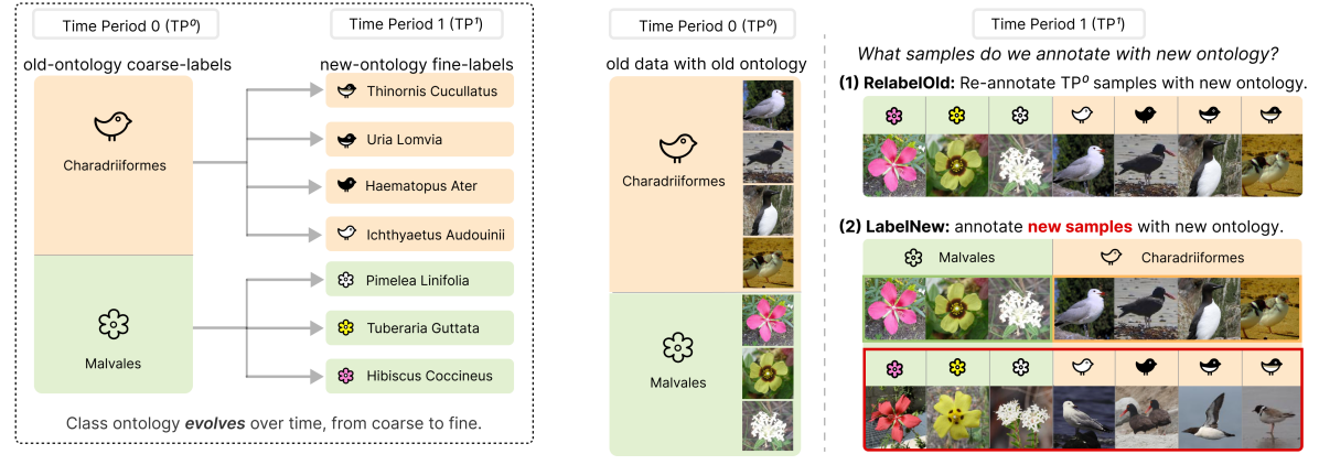
Figure 2: Left: Learning with Evolving Class Ontology (LECO) requires training models in time periods (TPs) that refine old ontologies in a coarse-to-fine fashion. This leads to a basic question: for the next TP, should one relabel the old data or label new data? Interestingly, both labeling protocols have been used in the community for large-scale datasets. Right: Our extensive experiments provide the (perhaps obvious) answer – one should always annotate new data with the new ontology rather than re-annotating the old. One reason is that the former produces more labeled data. Following this labeling protocol and to address LECO, we leverage insights from semi-supervised learning and learning-with-partial-labels to learn from such heterogenous annotations, approaching the upper bound of learning from an oracle aggregate dataset with all new labels.

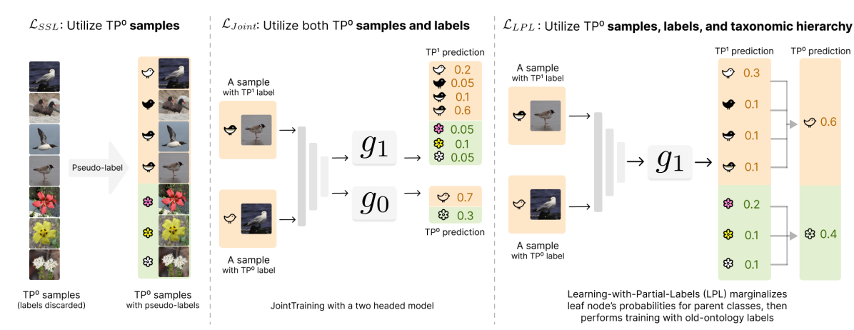
Figure 3: Visual illustration of LECO strategies. Left: $\mathcal{L}_{SSL}$ generates pseudo new-ontology/fine labels for old-ontology samples via semi-supervised learning (SSL). However, this ignores old-ontology/coarse labels which might serve as coarse-level supervision. We therefore advocate for $\mathcal{L}_{SSL/Filter}$ that filters out pseudo-labels with wrong coarse labels, or $\mathcal{L}_{SSL/Cond}$ that conditions leave’s probabilities based on the ground-truth parent/coarse class. Middle: $\mathcal{L}_{Joint}$ utilizes the old-ontology labels that come with the samples; to reconcile for different labels at different TPs, it trains a model with multiple classification heads. Right: $\mathcal{L}_{LPL}$ (learning-with-partial-labels) further utilizes the taxonomic hierarchy by exploiting the fact that newly added classes in LECO are refined from old classes. It does so by marginalizing leaves’ probabilties for their parent classes.

B: Rationale behind the selection of levels on iNaturalist

We repurpose the iNaturalist dataset to set up a LECO benchmarking protocol. The dataset has seven levels of taxa, allowing to use such as superclasses in LECO’s time periods. To determine the levels to use, we have two principles aiming to have a clean and challenging setup to study LECO. First, we think it is good to have more fine-grained classes in TP1, hence we choose the most fine-grained level “species” in TP1. Second, we think all coarse-classes should be split later to emphasize the difficulty of learning with class-evolution, and TP0’s classification task should be challenging as well with more classes. Therefore, we choose the “order” level which has 123 taxa. As reference, the original iNat dataset has seven levels: kingdom (3 taxa), phylum (8), class (29), order (123), family (339), genus (729), and species (810). The long-tailed class distributions in the two TPs are depicted in Fig. 4.

TP0 Distribution (123 classes)	TP1 Distribution (810 classes)
iNat-LECO Per-Class Image Distributions (Y-axis is log-scaled)

Figure 4: iNat-LECO Per-Class Distributions. We plot distributions of training images for iNat-LECO in log-scale. The x-axis are classes sorted by the number of images. The y-axis shows the number of images per class.

C: Experiments on Mapillary V1.2 $\rightarrow$ V2.0

As we briefly discussed in the main paper, Mapillary is a real-world example where a large dataset evolved over time from V1.2 [55] to V2.0 [52]. We include additional experiments on this real-world dataset versioning scenario. Mapillary is a rich and diverse street-level imagery dataset that was collected for semantic segmentation research in the context of autonomous driving. We repurpose this dataset for setting a LECO benchmark. Briefly, we use the ontology of Mapillary V1.2 in time period 1 (TP1), and V2.0 in TP2. TP1 has 66 classes including a catch-all background (aka void) class. TP1 (i.e., Mapillary V2.0 ) contains 124 classes, out of which 116 are used for evaluation.

Mapillary-LECO benchmark. The original Mapillary contains 18k training images, which is much larger than other mainstream street-level segmentation datasets such as Cityscape [14] (which has 2975 training and 500 validation images). In this work, we repurpose Mapillary to set up a LECO benchmark by splitting training set into two subsets (each containing 2.5k or 9k images) for the two time periods. We use the original validation set of Mapillary with 2k images as our test set. The detailed statistics is shown in Table 7.

Table 7: Mapillary-LECO statistics. We repurpose Mapillary [55, 52] V1.2 to V2.0 (a real-world dataset versioning scenario) to set up a LECO benchmark. Since V2.0 contains the same set of images as V1.2, in order to simulate a scenario with new samples, we select the first 5k or all 18k training images, then split them to 2.5k/9k for TP⁰ and 2.5k/9k for TP¹. Note that in TP⁰, the 66 classes include a catch-all background (or void) class, which is subsequently refined to 9 fine-grained classes such as traffic-cone and traffic-island.

dataset	Time Period 0 (TP0)			Time Period 1 (TP1)
	#classes	#train	#test	#classes	#train	#test
Mapillary-LECO	66	2.5k/9k	2k	116	2.5k/9k	2k

Baseline Experiments on Mapillary-LECO. We used the state-of-the-art architecture HRNet-V2-W48 for semantic segmentation with OCR module [72, 76, 81]. We noticed that for semantic segmentation on street-level imagery datasets [14], it is common to start from a Imagenet-pretrained model. Hence we name the weight initialization schemes for Mapillary-LECO as:

• (TrainRandom) Train an entire network from randomly initialized weights.

• (TrainScratch) Initialize the model backbone with ImageNet-pretrained weights.

As we can see from Table 8, TrainScratch (from ImageNet pretrained weights) as a popular initialization strategy for segmentation tasks [55, 14] indeed performs better than TrainRandom. Therefore, for our FinetunePrev strategy, we finetune the model checkpoint obtained via TrainScratch strategy on TP⁰ data. To further bridge the gap to AllFine, we experiment other advanced techniques introduced in this paper such as $\mathcal{L}_{SSL}$ and $\mathcal{L}_{Joint}$ as shown in Table 10.

Results of various LECO strategies. Since Mapillary does not reveal the taxonomic hierarchy from V1.2 to V2.0, we use the ground-truth label maps to automatically retrace the ontology evolution. Because Mapillary adopts RelabelOld strategy, each input image has both V1.2 and V2.0 label map. We exploit this fact to determine a single parent class in V1.2 for each of the 116 classes in V2.0 following a simple procedure (taking bird class in V2.0 as an example):

• First, we use the ground-truth V2.0 label maps to find all pixels labeled as bird.

• Then, we locate those pixels in V1.2 label maps, and choose the V1.2 class that occupies the most pixels as bird’s parent.

We find that this simple procedure produces a reliable taxonomic hierarchy that can be used to improve the performance via $\mathcal{L}_{LPL}$, $\mathcal{L}_{SSL/Filter}$ or $\mathcal{L}_{SSL/Cond}$, as shown in Table 11. Note that this procedure does not model class merging in Mapillary; however, our solutions still remain effective.

Segmentation Loss. We make use of a standard pixel-level cross-entropy loss function for training on Mapillary. One difference from our previous image classification setup is that both the ontology and semantic label maps changed from V1.2 to V2.0. In general, we find the label maps on V2.0 to be of higher quality. As such, we (1) do not add coarse supervision on TP¹ data ($\mathcal{B}_{K}$), since this pollutes the quality of annotations on the new data, i.e., $\mathcal{L}_{Joint}=\mathcal{L}_{old}(\mathcal{\hat{B}}_{M})$ and $\mathcal{L}_{LPL}=\mathcal{L}_{oldLPL}(\mathcal{\hat{B}}_{M})$, and (2) we mask out gradients on pixel regions (around $0.3\%$ of all pixels) where the given V1.2 labels do not align with the parent class of their V2.0 labels for $\mathcal{L}_{old}(\mathcal{\hat{B}}_{M})$ and $\mathcal{L}_{oldLPL}(\mathcal{\hat{B}}_{M})$.

Training and Inference Details. For both TrainRandom and TrainScratch, we use an initial learning rate of 0.03; for FinetunePrev, we use an initial learning rate of 0.003. The L2 weight decay is selected as 0.0005. Other hyperparameters followed the default strategy in HRNet used to achieve the SOTA results on Cityscape. We use SGD with 0.9 momentum and a batch size of 16 for $\mathcal{B}_{K}$ (or 8 for $\mathcal{B}_{K}$ and 8 for $\hat{\mathcal{B}}_{M}$ if we use $\mathcal{L}_{SSL}$ or $\mathcal{L}_{Joint}$). We use linear learning rate decay schedule that sets the learning rate to $\eta(1-\frac{k}{K})^{0.9}$ where $\eta$ is the initial learning rate and $k$/$K$ are the current and total iteration. For data augmentation, an input image and its label map are randomly flipped horizontally and then its longer edge will be scaled with a base size of 2200 pixels multiplied by a scalar factor sampled between 0.5 and 2.1. Finally, a 720x720 region will be randomly cropped for each of the 16 images in mini-batch for training. For inference, we use a sliding window of 720x720 without scaling of the image to determine the final pixel-level prediction. We also perform inference on the flipped image and take the average prediction as final result. Note that it is possible to use more advanced inference techniques such as multi-scaled testing, but we omit them to speed up inference since they are orthogonal to our research goal. We allocate the same training budget for all experiments. In particular, we use a total number of 1600 epochs for 2.5k/9k samples (a single TP), or 800 epochs for 5k/18k samples (two TPs data such as AllFine and LabelNew with SSL/Joint/LPL techniques). All experiments are conducted on internal clusters with 8 GeForce RTX 3090 cards.

Table 8: Results of baseline methods for Mapillary-LECO, analogous to Table 2 in the main paper. We report the mean Intersection-over-Union (mIoU in $\%$). TrainRandom trains a model from scratch, as is the protocol in the main paper. Because segmentation tasks typically make use of ImageNet pre-training, we also show results for TrainScratch that trains with an ImageNet-pretrained encoder, improving upon TrainRandom). Finally, FinetunePrev makes use of TP⁰’s model, which is trained with TrainScratch. In Table 10, we explore Joint-Training and SSL, leading to further improvement.

Benchmark	$\#$images / TP	TP1 Strategy	TP1 mIoU
			LabelNew	RelabelOld	AllFine
Mapillary-LECO	2500	TrainRandom	$27.24$	$27.21$	$27.73$
		TrainScratch	$28.22$	$29.28$	$30.71$
		FinetunePrev	30.39	$29.05$	$31.73$
Mapillary-LECO	9000	TrainScratch	$32.83$	$33.44$	$33.82$
		FinetunePrev	34.08	$35.01$	$36.20$

D: Dataset Statistics

TP0 Distribution (66 categories)	TP1 Distribution (116 categories)
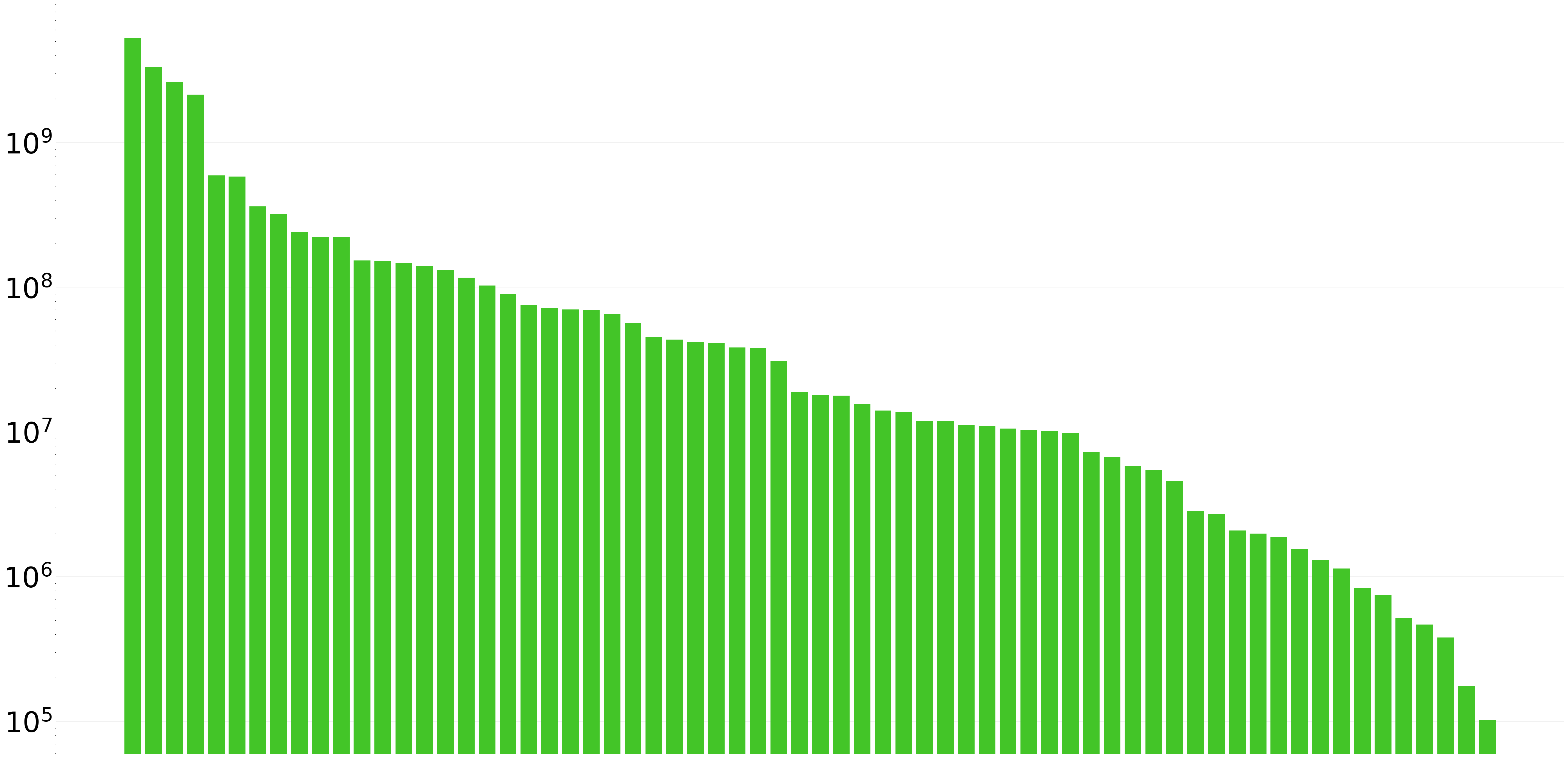
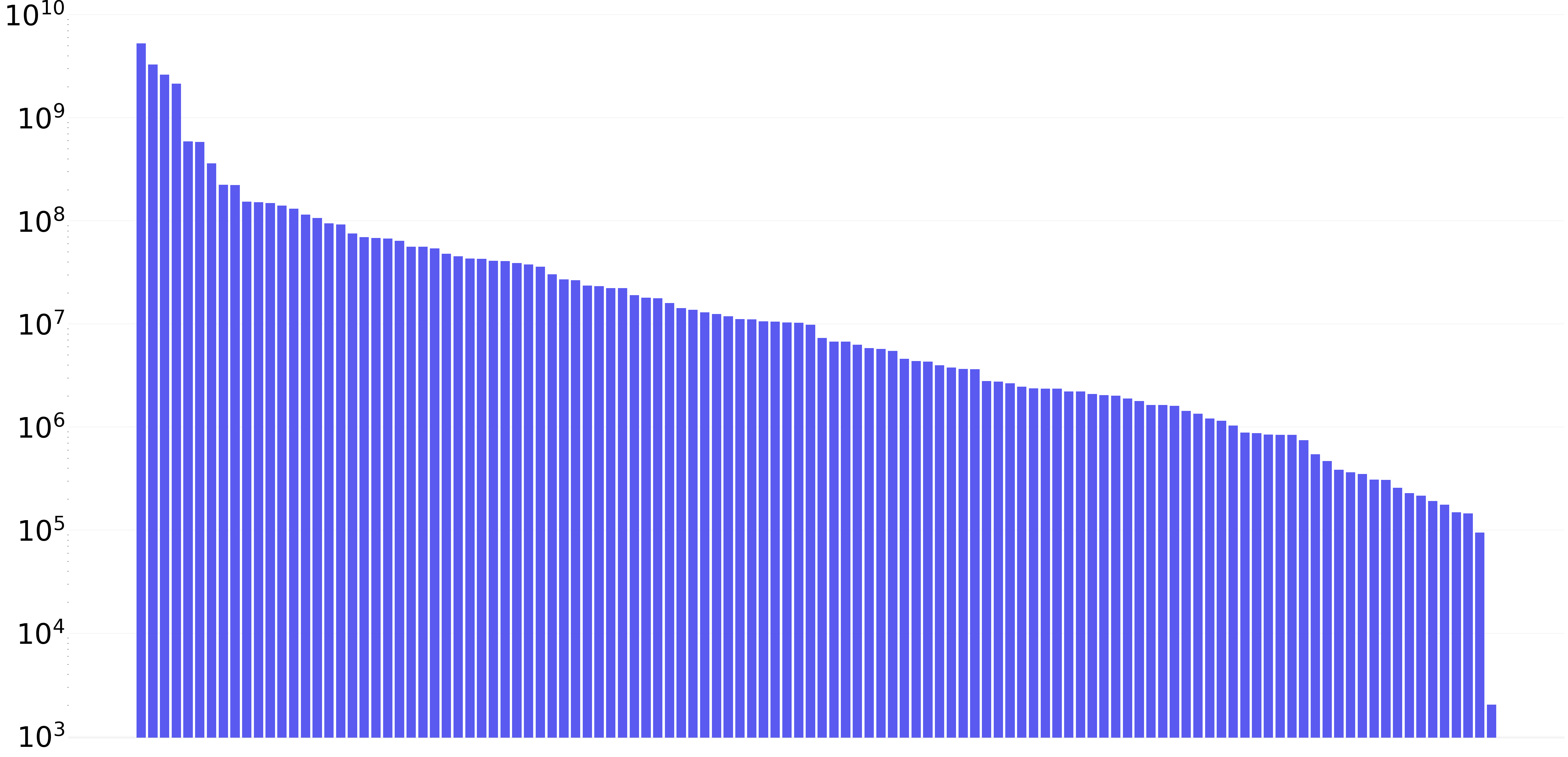
Mapillary-LECO Per-Class Pixel Distributions (Y-axis is log-scaled)

Figure 5: Mapillary-LECO Per-Class Distributions. We plot distributions of training pixels for iNat-LECO in log-scale. The x-axis are classes sorted by the number of pixels. The y-axis shows the number of pixels per class (in log scale).

To better understand the long-tailed nature of the datasets, we include the per-class image and pixel distributions for iNat-LECO in Figure 4 and Mapillary-LECO in Figure 5. We note that the long-tailed class distributions make semi-supervised methods less effective, as shown in Table 3,  4, 10, 11, e.g., the pseudo-labeling method of SSL underperforms the simple supervised learning baseline ($\mathcal{L}$ only).

E: Training Details on CIFAR-LECO and iNat-LECO

We include all training details for reproducibility in this section. We adopt SOTA training strategies from recent papers [68, 69, 70]. For all experiments, we train the CNN with mini-batch stochastic gradient descent with 0.9 momentum. Same as FixMatch [68], we use the an exponential moving average (EMA) of model parameters for final inference with a decay parameter of 0.999. We use a cosine annealing learning rate decay schedule which sets the learning rate to $\eta\cos{\frac{7\pi k}{16K}}$ where $\eta$ is the initial learning rate and $k$/$K$ are the current and total iteration. By default, we use a strong data augmentation scheme because it provides better generalization performance. In particular, we adopt RandAugment [16] as implemented in this repository. We did a grid search for best learning rate and weight decay using the validation set of each benchmark. The benchmark-specific hyperparameters are detailed below:

CIFAR100-LECO. We use the same model architecture (Wide-ResNet-28-2 [82]) in FixMatch paper for CIFAR100 experiments [68]. We use a batch size of 128 (if using $\mathcal{L}$ only), or we split the batch to 64 for $\mathcal{B}_{K}$ and 64 for $\hat{\mathcal{B}}_{M}$. For each experiment, we search for initial learning rate in $[0.6,0.06,0.006,0.0006]$ and report the best mAcc result. We use an L2 weight decay of 5e-4. We run for a total number of 160K iterations and evaluate on the validation set per 1K iterations (equivalent to around 2000 epochs for 10000 images).

iNat-LECO. We use the same model architecture (ResNet50 [28]) as in [70]. We use a batch size of 60 (if using $\mathcal{L}$ only), or we split the batch to 30 for $\mathcal{B}_{K}$ and 30 for $\hat{\mathcal{B}}_{M}$. Because it is a long-tailed recognition problem, we search for L2 weight decay as suggested by [2] in $[0.001,0.0001,0.00001]$ and found out 0.001 produces the best mAcc. Then for each experiment, we search for initial learning rate in $[0.01,0.001,0.0001]$ and report the best mAcc result. We run for a total number of 250K iterations and evaluate on the validation set per 1K iterations (equivalent to around 300 epochs for 50000 images).

iNat-4TP-LECO. The range of grid search of hyperparameters follows that of iNat-LECO, including 250K iterations (equivalent to around 600 epochs for 25000 images) for each TP.

All the classification experiments were performed on a single modern GPU card. Based on the batch size scale, we use different GPU types, e.g., GeForce RTX 2080 Ti for image classification on CIFAR and iNaturalist, and GeForce RTX 3090 Ti on Mapillary.

F: Comprehensive Experiment Results

We now show the complete results on varying sample sizes per TP for all benchmarks. Table 9,  10,  11 in appendix correspond to Table 2, 3, 4 in main paper. All conclusions generalize to varied number of samples and all 3 datasets.

We also have complete results using all combinations of the various SSL/Joint/LPL techniques introduced in main paper. Results can be found on Table 12 (CIFAR-LECO and iNat-LECO) and Table 13 (Mapillary-LECO).

Table 9: Results of baseline methods for LECO (complete results). For all our experiments except on Mapillary, we run each method five times and report the mean accuracy averaged over per-class accuracies with standard deviations. Because running on Mapillary is very compute-demanding, we run it once and report mean intersection-over-union (mIoU in $\%$) over per-class IoU. For each benchmark, we bold the best mAcc/mIoU including ties that fall within its std. All conclusions we derived in main paper still hold, e.g., FinetunePrev is the best learning strategy that outperforms TrainScratch (cf. 73.64% vs. 65.69% with LabelNew on iNat-LECO), implying that the coarse-to-fine evolved ontology serves as a good learning curriculum. FreezePrev significantly underperforms TrainScratch (cf. 50.82% vs. 65.69% with LabelNew on iNat-LECO), confirming the difficulty of learning new classes that refine the old. LabelNew and RelabelOld achieve similar performance with the former using only new data but not the old altogether. If using both old and new data, we boost performance as shown in Table 10. The conclusions hold for varied number of training images and generalize to the Mapillary experiments, yet all methods fall short to the AllFine (which trains on all data assumed to be labeled with new ontology).

Benchmark	$\#$images / TP	TP0 mAcc/mIoU	TP1 Strategy	TP1 mAcc/mIoU
				LabelNew	RelabelOld	AllFine
CIFAR-LECO	1000	$50.92\pm 0.89$	FinetunePrev	33.53 $\pm$ 0.57	$32.85\pm 0.47$	$42.27\pm 0.83$
			FreezePrev	$24.13\pm 0.67$	$24.70\pm 0.41$	$27.82\pm 0.43$
			TrainScratch	$30.88\pm 1.05$	$31.02\pm 0.68$	$41.74\pm 0.56$
CIFAR-LECO	2000	$59.48\pm 0.66$	FinetunePrev	43.44 $\pm$ 0.73	42.88 $\pm$ 0.72	$52.72\pm 0.38$
			FreezePrev	$33.74\pm 1.46$	$33.69\pm 1.44$	$36.57\pm 1.68$
			TrainScratch	$41.61\pm 0.53$	$41.77\pm 0.79$	$52.78\pm 0.35$
CIFAR-LECO	10000	$77.78\pm 0.27$	FinetunePrev	65.83 $\pm$ 0.53	65.30 $\pm$ 0.32	$71.30\pm 0.41$
			FreezePrev	$52.64\pm 0.50$	$52.60\pm 0.52$	$53.79\pm 0.43$
			TrainScratch	65.40 $\pm$ 0.53	$64.98\pm 0.34$	$71.43\pm 0.24$
iNat-LECO	50000	$64.21\pm 1.61$	FinetunePrev	73.64 $\pm$ 0.46	$71.26\pm 0.54$	$84.51\pm 0.66$
			FreezePrev	$50.82\pm 0.68$	$54.60\pm 0.49$	$54.08\pm 0.31$
			TrainScratch	$65.69\pm 0.46$	$65.78\pm 0.56$	$73.10\pm 0.80$
Mapillary-LECO	2500	$37.01$	FinetunePrev	30.39	$29.05$	$31.73$
			TrainScratch	$27.24$	$27.21$	$27.73$
Mapillary-LECO	9000	$44.14$	FinetunePrev	$34.08$	35.01	$36.20$
			TrainScratch	$32.83$	$33.44$	$33.82$

Table 10: Results of SSL and Joint Training methods (complete results). Following the notation of Table 9, we study LabelNew annotation strategies that make use of algorithms for learning from old examples without exploiting the relationship between old-vs-new labels. Recall that AllFine uses $\mathcal{L}$ only to train on all the data labeled with new ontology (doubling annotation cost). Using all the three losses together consistently improves mAcc / mIoU for all the benchmarks, confirming the benefit of exploiting the old examples. For instance, on iNat-LECO, this boosts the performance to $83.6\%$, approaching the AllFine ($84.5\%$)! Similar trends hold for Mapillary-LECO.

Benchmark	$\#$images / TP	SSL Alg	TP1 mAcc/mIoU
			$\mathcal{L}$ only	$+\mathcal{L}_{SSL}$	$+\mathcal{L}_{Joint}$	$+\mathcal{L}_{Joint}$ $+\mathcal{L}_{SSL}$	AllFine
CIFAR-LECO	1000	ST-Hard	$33.53\pm 0.57$	$34.59\pm 0.57$	$37.25\pm 0.66$	$35.27\pm 0.64$	$42.27\pm 0.83$
		ST-Soft		$37.67\pm 0.46$		38.48 $\pm$ 0.67
		PL		$33.53\pm 0.36$		$37.28\pm 0.67$
		FixMatch		$34.20\pm 0.24$		$37.47\pm 0.53$
CIFAR-LECO	2000	ST-Hard	$43.44\pm 0.73$	$44.87\pm 0.35$	$47.68\pm 0.70$	$45.67\pm 0.32$	$52.72\pm 0.38$
		ST-Soft		48.23 $\pm$ 0.55		48.72 $\pm$ 0.53
		PL		$43.46\pm 0.61$		$47.24\pm 0.40$
		FixMatch		$44.98\pm 0.59$		48.58 $\pm$ 0.71
CIFAR-LECO	10000	ST-Hard	$65.83\pm 0.27$	$67.11\pm 0.34$	$68.74\pm 0.21$	$67.97\pm 0.37$	$71.30\pm 0.41$
		ST-Soft		69.86 $\pm$ 0.30		69.77 $\pm$ 0.71
		PL		$65.86\pm 0.14$		$68.43\pm 0.40$
		FixMatch		$67.13\pm 0.36$		$69.03\pm 0.43$
iNat-LECO	50000	ST-Hard	$73.64\pm 0.46$	$75.23\pm 0.14$	$82.98\pm 0.33$	$78.23\pm 0.38$	$84.51\pm 0.66$
		ST-Soft		$79.64\pm 0.41$		83.61 $\pm$ 0.39
		PL		$73.56\pm 0.09$		$82.87\pm 0.51$
		FixMatch		$74.57\pm 0.54$		$83.00\pm 0.33$
Mapillary-LECO	2500	ST-Hard	$30.39$	$30.06$	31.05	31.09	$31.73$
Mapillary-LECO	9000	ST-Hard	$34.08$	$32.68$	35.40	35.72	$36.20$

Table 11: Results of exploiting taxonomic hierarchy (complete results). We copy the best results in Table 10 (all obtained by $+\mathcal{L}_{Joint}$ $+\mathcal{L}_{SSL}$) for reference. We can see that $\mathcal{L}_{LPL}$ is less effective but still competitive on Mapillary-LECO, presumably because it does not model the class-merging scenarios. Nonetheless, combinations of the strategies, i.e., adding SSL loss along with pseudo-label refinement via either Filtering or Conditioning still bridge the gap to AllFine.

Benchmark	$\#$images / TP	SSL Alg	TP1 mAcc
			$+\mathcal{L}_{Joint}$ $+\mathcal{L}_{SSL}$	$+\mathcal{L}_{LPL}$	$+\mathcal{L}_{LPL}$ $+\mathcal{L}_{SSL/Filter}$	$+\mathcal{L}_{LPL}$ $+\mathcal{L}_{SSL/Cond}$	AllFine
CIFAR-LECO	1000	ST-Hard	$38.48\pm 0.67$	38.47 $\pm$ 0.52	38.87 $\pm$ 0.54	38.68 $\pm$ 0.41	$42.27\pm 0.83$
		ST-Soft			38.87 $\pm$ 0.52	$38.19\pm 0.71$
		PL			38.56 $\pm$ 0.44	38.67 $\pm$ 0.81
		FixMatch			$37.55\pm 0.69$	$37.35\pm 0.72$
CIFAR-LECO	2000	ST-Hard	$48.72\pm 0.53$	$49.04\pm 0.47$	49.36 $\pm$ 0.56	$48.65\pm 0.53$	$52.72\pm 0.38$
		ST-Soft			$49.09\pm 0.46$	$48.54\pm 0.52$
		PL			49.25 $\pm$ 0.34	$48.91\pm 0.87$
		FixMatch			49.44 $\pm$ 0.22	$48.81\pm 0.40$
CIFAR-LECO	10000	ST-Hard	$69.77\pm 0.71$	$69.31\pm 0.30$	$69.90\pm 0.29$	70.42 $\pm$ 0.23	$71.30\pm 0.41$
		ST-Soft			$70.10\pm 0.12$	$70.02\pm 0.63$
		PL			$69.20\pm 0.20$	$69.60\pm 0.26$
		FixMatch			$69.61\pm 0.17$	$69.85\pm 0.46$
iNat-LECO	50000	ST-Hard	$83.61\pm 0.39$	$83.62\pm 0.21$	84.23 $\pm$ 0.61	84.34 $\pm$ 0.25	$84.51\pm 0.66$
		ST-Soft			84.12 $\pm$ 0.31	$83.76\pm 0.40$
		PL			$83.72\pm 0.22$	84.16 $\pm$ 0.19
		FixMatch			$83.91\pm 0.39$	$83.95\pm 0.40$
Mapillary-LECO	2500	ST-Hard	$31.09$	$31.04$	31.41	$31.23$	$31.73$
Mapillary-LECO	9000	ST-Hard	$35.72$	$35.04$	36.12	$35.47$	$36.20$

Table 12: Complete results of LECO strategies on classification benchmarks. We report results on combinations of all LECO stratgies on CIFAR100-LECO and iNat-LECO with FinetunePrev strategy on TP¹. Major conclusions hold across all benchmarks: (1) Utilizing old-ontology samples and labels, i.e., $\mathcal{L}_{SSL}$ and $\mathcal{L}_{Joint}$, helps bridge the gap to AllFine, and (2) exploiting taxonomic hierarchy via $\mathcal{L}_{SSL/Filter}$, $\mathcal{L}_{SSL/Cond}$, or $\mathcal{L}_{LPL}$ further improves the performance.

Setup

TP0 mAcc

TP1 mAcc

AllFine

LabelNew

No SSL

PL

FixMatch

ST-Hard

ST-Soft

$\mathcal{L}$

$\mathcal{L}_{LPL}$

$\mathcal{L}_{Joint}$

$\mathcal{L}$

$\mathcal{L}_{LPL}$

$\mathcal{L}_{Joint}$

$\mathcal{L}$

$\mathcal{L}_{LPL}$

$\mathcal{L}_{Joint}$

$\mathcal{L}$

$\mathcal{L}_{LPL}$

$\mathcal{L}_{Joint}$

$\mathcal{L}$

$\mathcal{L}_{LPL}$

$\mathcal{L}_{Joint}$

CIFAR100-1k

$50.92\pm 0.89$

$42.27\pm 0.83$

$33.53\pm 0.57$

$38.47\pm 0.52$

$37.25\pm 0.66$

+$\mathcal{L}_{SSL}$

$33.53\pm 0.36$

$38.70\pm 0.65$

$37.28\pm 0.67$

$34.20\pm 0.24$

$37.56\pm 0.54$

$37.47\pm 0.53$

$34.59\pm 0.57$

$36.78\pm 0.40$

$35.27\pm 0.64$

$37.67\pm 0.46$

$38.80\pm 0.49$

$38.48\pm 0.67$

+$\mathcal{L}_{SSL/Filter}$

$33.33\pm 0.69$

$38.56\pm 0.44$

$37.44\pm 0.84$

$36.02\pm 0.33$

$37.55\pm 0.69$

$37.23\pm 0.20$

$37.93\pm 0.50$

$38.87\pm 0.54$

$38.57\pm 0.74$

$37.59\pm 0.69$

$38.87\pm 0.52$

$38.43\pm 0.67$

+$\mathcal{L}_{SSL/Cond}$

$37.40\pm 1.19$

$38.67\pm 0.81$

$38.00\pm 0.59$

$36.92\pm 0.64$

$37.35\pm 0.72$

$37.08\pm 0.57$

$37.95\pm 0.34$

$38.68\pm 0.41$

$38.20\pm 0.30$

$38.25\pm 0.62$

$38.19\pm 0.71$

$38.45\pm 0.49$

CIFAR100-2k

$59.48\pm 0.66$

$52.72\pm 0.38$

$43.44\pm 0.73$

$49.04\pm 0.47$

$47.68\pm 0.70$

$\mathcal{L}_{SSL}$

$43.46\pm 0.61$

$48.82\pm 0.30$

$47.24\pm 0.40$

$44.98\pm 0.59$

$49.38\pm 0.29$

$48.58\pm 0.71$

$44.87\pm 0.35$

$46.98\pm 0.33$

$45.67\pm 0.32$

$48.23\pm 0.55$

$49.12\pm 0.50$

$48.72\pm 0.53$

$\mathcal{L}_{SSL/Filter}$

$43.50\pm 0.47$

$49.25\pm 0.34$

$47.38\pm 0.60$

$46.14\pm 0.33$

$49.44\pm 0.22$

$48.23\pm 1.21$

$47.00\pm 0.36$

$49.36\pm 0.56$

$49.01\pm 0.73$

$47.62\pm 0.74$

$49.09\pm 0.46$

$48.56\pm 0.50$

$\mathcal{L}_{SSL/Cond}$

$48.28\pm 0.27$

$48.91\pm 0.87$

$48.45\pm 0.34$

$48.23\pm 0.93$

$48.81\pm 0.40$

$48.57\pm 0.58$

$48.81\pm 0.57$

$48.65\pm 0.53$

$48.60\pm 0.68$

$48.70\pm 0.58$

$48.54\pm 0.52$

$48.86\pm 0.61$

CIFAR100-10k

$77.78\pm 0.27$

$71.30\pm 0.41$

$65.83\pm 0.27$

$69.31\pm 0.30$

$68.74\pm 0.21$

$\mathcal{L}_{SSL}$

$65.86\pm 0.14$

$69.48\pm 0.24$

$68.43\pm 0.40$

$67.13\pm 0.36$

$69.71\pm 0.49$

$69.03\pm 0.43$

$67.11\pm 0.34$

$68.58\pm 0.51$

$67.97\pm 0.37$

$69.86\pm 0.30$

$68.96\pm 0.27$

$69.77\pm 0.71$

$\mathcal{L}_{SSL/Filter}$

$65.80\pm 0.34$

$69.20\pm 0.20$

$68.82\pm 0.23$

$67.60\pm 0.25$

$69.61\pm 0.17$

$69.15\pm 0.41$

$69.04\pm 0.29$

$69.90\pm 0.29$

$69.95\pm 0.28$

$68.76\pm 0.20$

$70.10\pm 0.12$

$69.85\pm 0.38$

$\mathcal{L}_{SSL/Cond}$

$68.32\pm 0.26$

$69.60\pm 0.26$

$69.09\pm 0.13$

$68.86\pm 0.52$

$69.85\pm 0.46$

$69.41\pm 0.39$

$70.22\pm 0.38$

$70.42\pm 0.23$

$70.05\pm 0.18$

$70.33\pm 0.15$

$70.02\pm 0.63$

$69.93\pm 0.24$

iNat-50k

$64.21\pm 1.61$

$84.51\pm 0.66$

$73.64\pm 0.46$

$83.62\pm 0.21$

$82.98\pm 0.33$

$\mathcal{L}_{SSL}$

$73.56\pm 0.09$

$83.71\pm 0.44$

$82.87\pm 0.51$

$74.57\pm 0.54$

$84.05\pm 0.26$

$83.00\pm 0.33$

$75.23\pm 0.14$

$79.07\pm 0.48$

$78.23\pm 0.38$

$79.64\pm 0.41$

$84.10\pm 0.54$

$83.61\pm 0.39$

$\mathcal{L}_{SSL/Filter}$

$74.01\pm 0.41$

$83.72\pm 0.22$

$82.81\pm 0.27$

$74.55\pm 0.33$

$83.91\pm 0.39$

$83.16\pm 0.33$

$79.91\pm 0.58$

$84.23\pm 0.61$

$83.92\pm 0.25$

$78.71\pm 0.22$

$84.12\pm 0.31$

$83.80\pm 0.60$

$\mathcal{L}_{SSL/Cond}$

$81.98\pm 0.12$

$84.16\pm 0.19$

$82.99\pm 0.64$

$82.62\pm 0.21$

$83.95\pm 0.40$

$83.66\pm 0.36$

$84.20\pm 0.29$

$84.34\pm 0.25$

$84.37\pm 0.39$

$83.96\pm 0.47$

$83.76\pm 0.40$

$83.95\pm 0.20$

Table 13: Complete results of LECO strategies on Mapillary-LECO. We report results on combinations of all LECO stratgies on Mapillary-LECO with FinetunePrev strategy on TP¹. It is worth noting that new labels in V2.0 do not necessarily have surjective mappings to old labels of V1.2. This means, it is non-trivial to apply coarse supervision as partial labels. Moreover, we only perform ST-Hard for SSL because other methods are excessively compute-demanding (e.g., ST-SOft requires saving per-class heatmaps for each image to allow making use of pseudo-labels’ scores, FixMatch requires learning a separate large-scale model, etc.). Concretely, we (1) do not add coarse supervision for $\mathcal{B}_{K}$ since it pollutes quality of annotation on new data, and (2) mask out gradient where the given V1.2 labels do not align with the parent class for $\mathcal{L}_{old}(\hat{\mathcal{B}}_{M})$ and $\mathcal{L}_{oldLPL}(\hat{\mathcal{B}}_{M})$. Major conclusions hold here. We can see that all combinations of various LECO stratgies achieve suprisingly good performances, whereas the best combination bridges $95\%$ of the gap to AllFine (gap reduces from 1.34 to 0.08 for 2.5k samples with $\mathcal{L}_{SSL}$ and $\mathcal{L}_{LPL}$, and from 2.12 to 0.08 for 9k samples with $\mathcal{L}_{SSL/Filter}$ and $\mathcal{L}_{LPL}$).

Setup	TP0 mIoU	TP1 mIoU
		AllFine	LabelNew
			No SSL				ST-Hard
			$\mathcal{L}$	$\mathcal{L}_{LPL}$	$\mathcal{L}_{Joint}$		$\mathcal{L}$	$\mathcal{L}_{LPL}$	$\mathcal{L}_{Joint}$
Mapillary-2.5k	$37.01$	$31.73$	$30.39$	$31.04$	$31.05$	+$\mathcal{L}_{SSL}$	$30.06$	$31.65$	$31.09$
						+$\mathcal{L}_{SSL/Filter}$	$30.64$	$31.41$	$31.57$
						+$\mathcal{L}_{SSL/Cond}$	$31.01$	$31.23$	$31.50$
Mapillary-9k	$44.14$	$36.20$	$34.08$	$35.04$	$35.40$	+$\mathcal{L}_{SSL}$	$32.68$	$35.97$	$35.72$
						+$\mathcal{L}_{SSL/Filter}$	$34.96$	$36.12$	$36.06$
						+$\mathcal{L}_{SSL/Cond}$	$35.29$	$35.47$	$35.70$

References

- Abdelsalam et al. [2021] Abdelsalam, M., Faramarzi, M., Sodhani, S., and Chandar, S. (2021). Iirc: Incremental implicitly-refined classification. In Proceedings of the IEEE/CVF Conference on Computer Vision and Pattern Recognition, pages 11038–11047.
- Alshammari et al. [2022] Alshammari, S., Wang, Y., Ramanan, D., and Kong, S. (2022). Long-tailed recognition via weight balancing. In CVPR.
- Azizpour et al. [2015] Azizpour, H., Razavian, A. S., Sullivan, J., Maki, A., and Carlsson, S. (2015). Factors of transferability for a generic convnet representation. IEEE transactions on pattern analysis and machine intelligence, 38(9), 1790–1802.
- Behley et al. [2019] Behley, J., Garbade, M., Milioto, A., Quenzel, J., Behnke, S., Stachniss, C., and Gall, J. (2019). Semantickitti: A dataset for semantic scene understanding of lidar sequences. In ICCV.
- Bengio et al. [2009] Bengio, Y., Louradour, J., Collobert, R., and Weston, J. (2009). Curriculum learning. In Proceedings of the 26th annual international conference on machine learning, pages 41–48.
- Berthelot et al. [2019a] Berthelot, D., Carlini, N., Goodfellow, I., Papernot, N., Oliver, A., and Raffel, C. A. (2019a). Mixmatch: A holistic approach to semi-supervised learning. NeurIPS, 32.
- Berthelot et al. [2019b] Berthelot, D., Carlini, N., Cubuk, E. D., Kurakin, A., Sohn, K., Zhang, H., and Raffel, C. (2019b). Remixmatch: Semi-supervised learning with distribution alignment and augmentation anchoring. arXiv preprint arXiv:1911.09785.
- Bertinetto et al. [2020] Bertinetto, L., Mueller, R., Tertikas, K., Samangooei, S., and Lord, N. A. (2020). Making better mistakes: Leveraging class hierarchies with deep networks. In CVPR.
- Bucak et al. [2011] Bucak, S. S., Jin, R., and Jain, A. K. (2011). Multi-label learning with incomplete class assignments. In CVPR 2011, pages 2801–2808. IEEE.
- Cai et al. [2021] Cai, Z., Sener, O., and Koltun, V. (2021). Online continual learning with natural distribution shifts: An empirical study with visual data. In Proceedings of the IEEE/CVF International Conference on Computer Vision, pages 8281–8290.
- Caruana [1997] Caruana, R. (1997). Multitask learning. Machine learning, 28(1), 41–75.
- Chang et al. [2019] Chang, M.-F., Lambert, J., Sangkloy, P., Singh, J., Bak, S., Hartnett, A., Wang, D., Carr, P., Lucey, S., Ramanan, D., et al. (2019). Argoverse: 3d tracking and forecasting with rich maps. In Proceedings of the IEEE/CVF Conference on Computer Vision and Pattern Recognition, pages 8748–8757.
- Cohen et al. [2022] Cohen, N., Gal, R., Meirom, E. A., Chechik, G., and Atzmon, Y. (2022). " this is my unicorn, fluffy": Personalizing frozen vision-language representations. arXiv preprint arXiv:2204.01694.
- Cordts et al. [2016] Cordts, M., Omran, M., Ramos, S., Rehfeld, T., Enzweiler, M., Benenson, R., Franke, U., Roth, S., and Schiele, B. (2016). The cityscapes dataset for semantic urban scene understanding. In CVPR.
- Cour et al. [2011] Cour, T., Sapp, B., and Taskar, B. (2011). Learning from partial labels. The Journal of Machine Learning Research, 12, 1501–1536.
- Cubuk et al. [2020] Cubuk, E. D., Zoph, B., Shlens, J., and Le, Q. V. (2020). Randaugment: Practical automated data augmentation with a reduced search space. In Proceedings of the IEEE/CVF Conference on Computer Vision and Pattern Recognition Workshops, pages 702–703.
- De Lange et al. [2021] De Lange, M., Aljundi, R., Masana, M., Parisot, S., Jia, X., Leonardis, A., Slabaugh, G., and Tuytelaars, T. (2021). A continual learning survey: Defying forgetting in classification tasks. IEEE transactions on pattern analysis and machine intelligence, 44(7), 3366–3385.
- Delange et al. [2021] Delange, M., Aljundi, R., Masana, M., Parisot, S., Jia, X., Leonardis, A., Slabaugh, G., and Tuytelaars, T. (2021). A continual learning survey: Defying forgetting in classification tasks. PAMI.
- Deng et al. [2014] Deng, J., Ding, N., Jia, Y., Frome, A., Murphy, K., Bengio, S., Li, Y., Neven, H., and Adam, H. (2014). Large-scale object classification using label relation graphs. In European conference on computer vision, pages 48–64. Springer.
- Donahue et al. [2014] Donahue, J., Jia, Y., Vinyals, O., Hoffman, J., Zhang, N., Tzeng, E., and Darrell, T. (2014). Decaf: A deep convolutional activation feature for generic visual recognition. In International conference on machine learning, pages 647–655. PMLR.
- Elman [1993] Elman, J. L. (1993). Learning and development in neural networks: The importance of starting small. Cognition, 48(1), 71–99.
- Everingham et al. [2015] Everingham, M., Eslami, S. A., Van Gool, L., Williams, C. K., Winn, J., and Zisserman, A. (2015). The pascal visual object classes challenge: A retrospective. IJCV, 111(1), 98–136.
- Geiger et al. [2012] Geiger, A., Lenz, P., and Urtasun, R. (2012). Are we ready for autonomous driving? the kitti vision benchmark suite. In 2012 IEEE conference on computer vision and pattern recognition, pages 3354–3361. IEEE.
- Gidaris et al. [2019] Gidaris, S., Bursuc, A., Komodakis, N., Pérez, P., and Cord, M. (2019). Boosting few-shot visual learning with self-supervision. In Proceedings of the IEEE/CVF International Conference on Computer Vision, pages 8059–8068.
- Goel et al. [2022] Goel, A., Fernando, B., Keller, F., and Bilen, H. (2022). Not all relations are equal: Mining informative labels for scene graph generation. In Proceedings of the IEEE/CVF Conference on Computer Vision and Pattern Recognition, pages 15596–15606.
- Grandvalet et al. [2004] Grandvalet, Y., Bengio, Y., et al. (2004). Learning from partial labels with minimum entropy. Technical report, CIRANO.
- Gupta et al. [2019] Gupta, A., Dollar, P., and Girshick, R. (2019). Lvis: A dataset for large vocabulary instance segmentation. In Proceedings of the IEEE/CVF Conference on Computer Vision and Pattern Recognition, pages 5356–5364.
- He et al. [2016] He, K., Zhang, X., Ren, S., and Sun, J. (2016). Deep residual learning for image recognition. In CVPR.
- Hinton et al. [2015] Hinton, G., Vinyals, O., and Dean, J. (2015). Distilling the knowledge in a neural network. arXiv preprint arXiv:1503.02531.
- Houlsby et al. [2019] Houlsby, N., Giurgiu, A., Jastrzebski, S., Morrone, B., De Laroussilhe, Q., Gesmundo, A., Attariyan, M., and Gelly, S. (2019). Parameter-efficient transfer learning for nlp. In International Conference on Machine Learning, pages 2790–2799. PMLR.
- Hsieh et al. [2019] Hsieh, C.-Y., Xu, M., Niu, G., Lin, H.-T., and Sugiyama, M. (2019). A pseudo-label method for coarse-to-fine multi-label learning with limited supervision.
- Hu et al. [2018] Hu, P., Lipton, Z. C., Anandkumar, A., and Ramanan, D. (2018). Active learning with partial feedback. arXiv preprint arXiv:1802.07427.
- iNaturalist 2017 [2017] iNaturalist 2017 (2017). https://www.inaturalist.org/stats/2017.
- iNaturalist 2018 [2018] iNaturalist 2018 (2018). https://www.inaturalist.org/stats/2018.
- iNaturalist 2019 [2019] iNaturalist 2019 (2019). https://www.inaturalist.org/stats/2019.
- iNaturalist 2020 [2020] iNaturalist 2020 (2020). https://www.inaturalist.org/stats/2020.
- iNaturalist 2021 [2021] iNaturalist 2021 (2021). https://www.inaturalist.org/stats/2021.
- Jia et al. [2022] Jia, M., Tang, L., Chen, B.-C., Cardie, C., Belongie, S., Hariharan, B., and Lim, S.-N. (2022). Visual prompt tuning. arXiv preprint arXiv:2203.12119.
- Kang et al. [2020] Kang, B., Xie, S., Rohrbach, M., Yan, Z., Gordo, A., Feng, J., and Kalantidis, Y. (2020). Decoupling representation and classifier for long-tailed recognition. In International Conference on Learning Representations.
- Kirkpatrick et al. [2017] Kirkpatrick, J., Pascanu, R., Rabinowitz, N., Veness, J., Desjardins, G., Rusu, A. A., Milan, K., Quan, J., Ramalho, T., Grabska-Barwinska, A., et al. (2017). Overcoming catastrophic forgetting in neural networks. Proceedings of the national academy of sciences, 114(13), 3521–3526.
- Kong and Ramanan [2021] Kong, S. and Ramanan, D. (2021). Opengan: Open-set recognition via open data generation. In Proceedings of the IEEE/CVF International Conference on Computer Vision, pages 813–822.
- Krizhevsky et al. [2009] Krizhevsky, A., Hinton, G., et al. (2009). Learning multiple layers of features from tiny images.
- Krueger and Dayan [2009] Krueger, K. A. and Dayan, P. (2009). Flexible shaping: How learning in small steps helps. Cognition, 110(3), 380–394.
- Lee et al. [2013] Lee, D.-H. et al. (2013). Pseudo-label: The simple and efficient semi-supervised learning method for deep neural networks. In Workshop on challenges in representation learning, ICML, volume 3, page 896.
- Lei et al. [2017] Lei, J., Guo, Z., and Wang, Y. (2017). Weakly supervised image classification with coarse and fine labels. In 2017 14th Conference on Computer and Robot Vision (CRV), pages 240–247. IEEE.
- Li et al. [2022] Li, W.-H., Liu, X., and Bilen, H. (2022). Cross-domain few-shot learning with task-specific adapters. In Proceedings of the IEEE/CVF Conference on Computer Vision and Pattern Recognition, pages 7161–7170.
- Li and Hoiem [2017] Li, Z. and Hoiem, D. (2017). Learning without forgetting. IEEE transactions on pattern analysis and machine intelligence, 40(12), 2935–2947.
- Lin et al. [2014] Lin, T.-Y., Maire, M., Belongie, S., Hays, J., Perona, P., Ramanan, D., Dollár, P., and Zitnick, C. L. (2014). Microsoft coco: Common objects in context. In ECCV. Springer.
- Lin et al. [2021] Lin, Z., Shi, J., Pathak, D., and Ramanan, D. (2021). The clear benchmark: Continual learning on real-world imagery. In Thirty-fifth Conference on Neural Information Processing Systems Datasets and Benchmarks Track (Round 2).
- Lomonaco and Maltoni [2017] Lomonaco, V. and Maltoni, D. (2017). Core50: a new dataset and benchmark for continuous object recognition. In Conference on Robot Learning, pages 17–26. PMLR.
- Maltoni and Lomonaco [2019] Maltoni, D. and Lomonaco, V. (2019). Continuous learning in single-incremental-task scenarios. Neural Networks, 116, 56–73.
- Mapillary-Vistas-2.0 [2021] Mapillary-Vistas-2.0 (2021). https://blog.mapillary.com/update/2021/01/18/vistas-2-dataset.html.
- Marszalek and Schmid [2007] Marszalek, M. and Schmid, C. (2007). Semantic hierarchies for visual object recognition. In 2007 IEEE Conference on Computer Vision and Pattern Recognition, pages 1–7. IEEE.
- McLachlan [1975] McLachlan, G. J. (1975). Iterative reclassification procedure for constructing an asymptotically optimal rule of allocation in discriminant analysis. Journal of the American Statistical Association, 70(350), 365–369.
- Neuhold et al. [2017] Neuhold, G., Ollmann, T., Rota Bulo, S., and Kontschieder, P. (2017). The mapillary vistas dataset for semantic understanding of street scenes. In Proceedings of the IEEE international conference on computer vision, pages 4990–4999.
- Nguyen and Caruana [2008] Nguyen, N. and Caruana, R. (2008). Classification with partial labels. In Proceedings of the 14th ACM SIGKDD international conference on Knowledge discovery and data mining, pages 551–559.
- Peterson [2004] Peterson, G. B. (2004). A day of great illumination: Bf skinner’s discovery of shaping. Journal of the experimental analysis of behavior, 82(3), 317–328.
- Phoo and Hariharan [2021] Phoo, C. P. and Hariharan, B. (2021). Coarsely-labeled data for better few-shot transfer. In Proceedings of the IEEE/CVF International Conference on Computer Vision, pages 9052–9061.
- Prabhu et al. [2020] Prabhu, A., Torr, P. H., and Dokania, P. K. (2020). Gdumb: A simple approach that questions our progress in continual learning. In ECCV.
- Rebuffi et al. [2017] Rebuffi, S.-A., Kolesnikov, A., Sperl, G., and Lampert, C. H. (2017). icarl: Incremental classifier and representation learning. In Proceedings of the IEEE conference on Computer Vision and Pattern Recognition, pages 2001–2010.
- Ristin et al. [2015] Ristin, M., Gall, J., Guillaumin, M., and Van Gool, L. (2015). From categories to subcategories: large-scale image classification with partial class label refinement. In Proceedings of the IEEE conference on computer vision and pattern recognition, pages 231–239.
- Rizve et al. [2021] Rizve, M. N., Duarte, K., Rawat, Y. S., and Shah, M. (2021). In defense of pseudo-labeling: An uncertainty-aware pseudo-label selection framework for semi-supervised learning. arXiv preprint arXiv:2101.06329.
- Sanger [1994] Sanger, T. D. (1994). Neural network learning control of robot manipulators using gradually increasing task difficulty. IEEE transactions on Robotics and Automation, 10(3), 323–333.
- Sariyildiz et al. [2021] Sariyildiz, M. B., Kalantidis, Y., Larlus, D., and Alahari, K. (2021). Concept generalization in visual representation learning. In Proceedings of the IEEE/CVF International Conference on Computer Vision, pages 9629–9639.
- Scudder [1965] Scudder, H. (1965). Probability of error of some adaptive pattern-recognition machines. IEEE Transactions on Information Theory, 11(3), 363–371.
- Sharif Razavian et al. [2014] Sharif Razavian, A., Azizpour, H., Sullivan, J., and Carlsson, S. (2014). Cnn features off-the-shelf: an astounding baseline for recognition. In Proceedings of the IEEE conference on computer vision and pattern recognition workshops, pages 806–813.
- Skinner [1958] Skinner, B. F. (1958). Reinforcement today. American Psychologist, 13(3), 94.
- Sohn et al. [2020] Sohn, K., Berthelot, D., Carlini, N., Zhang, Z., Zhang, H., Raffel, C. A., Cubuk, E. D., Kurakin, A., and Li, C.-L. (2020). Fixmatch: Simplifying semi-supervised learning with consistency and confidence. NeurIPS.
- Su and Maji [2021a] Su, J. and Maji, S. (2021a). Semi-supervised learning with taxonomic labels. In British Machine Vision Conference (BMVC).
- Su et al. [2021] Su, J., Cheng, Z., and Maji, S. (2021). A realistic evaluation of semi-supervised learning for fine-grained classification. In IEEE Conference on Computer Vision and Pattern Recognition (CVPR).
- Su and Maji [2021b] Su, J.-C. and Maji, S. (2021b). The semi-supervised inaturalist challenge at the fgvc8 workshop. arXiv preprint arXiv:2106.01364.
- Sun et al. [2019] Sun, K., Xiao, B., Liu, D., and Wang, J. (2019). Deep high-resolution representation learning for human pose estimation. In CVPR.
- Taherkhani et al. [2019] Taherkhani, F., Kazemi, H., Dabouei, A., Dawson, J., and Nasrabadi, N. M. (2019). A weakly supervised fine label classifier enhanced by coarse supervision. In Proceedings of the IEEE/CVF International Conference on Computer Vision, pages 6459–6468.
- Van de Ven and Tolias [2019] Van de Ven, G. M. and Tolias, A. S. (2019). Three scenarios for continual learning. arXiv preprint arXiv:1904.07734.
- Van Horn et al. [2018] Van Horn, G., Mac Aodha, O., Song, Y., Cui, Y., Sun, C., Shepard, A., Adam, H., Perona, P., and Belongie, S. (2018). The inaturalist species classification and detection dataset. In Proceedings of the IEEE conference on computer vision and pattern recognition, pages 8769–8778.
- Wang et al. [2019] Wang, J., Sun, K., Cheng, T., Jiang, B., Deng, C., Zhao, Y., Liu, D., Mu, Y., Tan, M., Wang, X., Liu, W., and Xiao, B. (2019). Deep high-resolution representation learning for visual recognition. TPAMI.
- Wang et al. [2022] Wang, X., Wu, Z., Lian, L., and Yu, S. X. (2022). Debiased learning from naturally imbalanced pseudo-labels. In Proceedings of the IEEE/CVF Conference on Computer Vision and Pattern Recognition, pages 14647–14657.
- Wilson et al. [2021] Wilson, B., Qi, W., Agarwal, T., Lambert, J., Singh, J., Khandelwal, S., Pan, B., Kumar, R., Hartnett, A., Pontes, J. K., et al. (2021). Argoverse 2: Next generation datasets for self-driving perception and forecasting.
- Xie et al. [2020] Xie, Q., Luong, M.-T., Hovy, E., and Le, Q. V. (2020). Self-training with noisy student improves imagenet classification. In Proceedings of the IEEE/CVF conference on computer vision and pattern recognition, pages 10687–10698.
- Yosinski et al. [2014] Yosinski, J., Clune, J., Bengio, Y., and Lipson, H. (2014). How transferable are features in deep neural networks? NeurIPS.
- Yuan et al. [2020] Yuan, Y., Chen, X., and Wang, J. (2020). Object-contextual representations for semantic segmentation.
- Zagoruyko and Komodakis [2016] Zagoruyko, S. and Komodakis, N. (2016). Wide residual networks. arXiv preprint arXiv:1605.07146.
- Zenke et al. [2017] Zenke, F., Poole, B., and Ganguli, S. (2017). Continual learning through synaptic intelligence. In ICML.
- Zhai et al. [2019] Zhai, X., Oliver, A., Kolesnikov, A., and Beyer, L. (2019). S4l: Self-supervised semi-supervised learning. In Proceedings of the IEEE/CVF International Conference on Computer Vision, pages 1476–1485.
- Zhang et al. [2018] Zhang, H., Cisse, M., Dauphin, Y. N., and Lopez-Paz, D. (2018). mixup: Beyond empirical risk minimization. In International Conference on Learning Representations.
- Zhang et al. [2020a] Zhang, J., Zhang, J., Ghosh, S., Li, D., Tasci, S., Heck, L., Zhang, H., and Kuo, C.-C. J. (2020a). Class-incremental learning via deep model consolidation. In Proceedings of the IEEE/CVF Winter Conference on Applications of Computer Vision, pages 1131–1140.
- Zhang et al. [2020b] Zhang, J. O., Sax, A., Zamir, A., Guibas, L., and Malik, J. (2020b). Side-tuning: a baseline for network adaptation via additive side networks. In European Conference on Computer Vision, pages 698–714. Springer.
- Zweig and Weinshall [2007] Zweig, A. and Weinshall, D. (2007). Exploiting object hierarchy: Combining models from different category levels. In 2007 IEEE 11th international conference on computer vision, pages 1–8. IEEE.