On Distributed Detection in EH-WSNs With Finite-State Markov Channel and Limited Feedback

Abstract

We consider a network, tasked with solving binary distributed detection, consisting of $N$ sensors, a fusion center (FC), and a feedback channel from the FC to sensors. Each sensor is capable of harvesting energy and is equipped with a finite size battery to store randomly arrived energy. Sensors process their observations and transmit their symbols to the FC over orthogonal fading channels. The FC fuses the received symbols and makes a global binary decision. We aim at developing adaptive channel-dependent transmit power control policies such that $J$-divergence based detection metric is maximized at the FC, subject to total transmit power constraint. Modeling the quantized fading channel, the energy arrival, and the battery dynamics as time-homogeneous finite-state Markov chains, and the network lifetime as a geometric random variable, we formulate our power control optimization problem as a discounted infinite-horizon constrained Markov decision process (MDP) problem, where sensors’ transmit powers are functions of the battery states, quantized channel gains, and the arrived energies. We utilize stochastic dynamic programming and Lagrangian approach to find the optimal and sub-optimal power control policies. We demonstrate that our sub-optimal policy provides a close-to-optimal performance with a reduced computational complexity and without imposing signaling overhead on sensors.

I Introduction

Event detection for smarter cities, healthcare systems, farming, and greenhouse environmental monitoring systems is one of the vital tasks in wireless sensor networks (WSNs) [1, 2] and the Internet of things (IoT)-based WSNs [3, 4]. The classical studies of binary distributed detection in [5, 6, 7] cannot be directly applied to these networks, since the classical works are based on the assumption that the rate-constrained communication channels between distributed sensors and fusion center (FC) are error-free. This has motivated researchers to study channel-dependent local decision rules for sensors and decision fusion rules for the FC, such that the effect of wireless communication channels in WSNs is integrated into the system designs [8, 9, 10, 11]. Even for channel-dependent distributed detection system designs, providing a guaranteed detection performance by a conventional WSN, in which sensors are powered by conventional non-rechargeable batteries and become inactive when the stored energy in their batteries is exhausted, is impossible. Although adaptive signal transmission strategies, including optimal channel-dependent power control [12, 13, 14] and censoring [15, 16], can enhance the energy efficiency and increase the lifetime of a conventional WSN, they cannot change the fact that the network lifetime is inherently limited. This limited lifetime disrupts the event detection task and drastically degrades the detection performance.

Energy harvesting (EH) from the environment is a promising solution to address the energy constraint problem in conventional WSNs, and to render these networks to self sustainable networks with perpetual lifetimes. The new class of EH-powered WSNs, where nodes have EH capability and are equipped with rechargeable batteries, will be also important for the development of IoT-based WSNs. In EH-powered WSNs power/energy management is necessary, in order to balance the rates of energy harvesting and energy consumption for transmission. If the energy management policy is overly aggressive, sensors may stop functioning, due to energy outage. On the other hand, if the policy is overly conservative, sensors may fail to utilize the excess energy, due to energy overflow, leading into a performance degradation. EH has been also considered in the contexts of data communications [17, 18], cognitive radio systems [19], distributed estimation [20], and distributed detection [21, 22, 23, 24, 25, 26, 27]. The body of research on EH-enabled communication systems can be grouped into two main categories, depending on the adopted energy arrival model [18, 28]: in deterministic models the transmitter has full (causal and non-causal) knowledge of energy arrival instants and amounts at the beginning of transmission, in stochastic models, suitable for modeling ambient RF and renewable energy sources that are intrinsically time-variant and sporadic, the transmitter only has causal knowledge of energy arrival. In addition, wireless communication channels change randomly in time due to fading. These together prompt the need for developing new power control/energy scheduling strategies for an EH-enabled transmitter that can best exploit and adapt to the random energy arrivals and time-varying fading channels.

Designing power control/energy scheduling schemes corresponding to random energy arrivals and time-varying fading channels can be viewed as a multistage stochastic optimization problem, where the goal is to find a sequence of decisions a decision maker has to make, such that a specific metric over a horizon spanning several time slots is optimized (e.g., optimizing transmission completion time, data throughput, outage probability, or symbol error rate in a point-to-point EH-powered wireless communication system [18]). A common approach to solve this sequential decision making problem is to adopt the mathematical framework of Markov decision processes (MDP). The main ingredients of the MDP are states, actions, rewards, and state transition probabilities. The state could be a composite states of fading channel, energy arrival, and battery condition. The action is the transmit power level or the amount of energy to be consumed, and the reward is a function of the states and the actions. The state transition probability describes the transition probability from the current state to the next state with respect to each action. The goal is to find the optimal policy, which specifies the optimal action in the state and maximizes the long-term expected discount infinite-horizon reward starting from the initial state [18].

In the context of distributed detection in WSNs, there are only few studies that consider EH-powered sensors [21, 22, 23, 24, 25, 26, 27]. In the following we provide a concise review of these works, highlight how our present work fills the knowledge gap in the literature, and how it is different from our previous works in [25, 26, 27].

I-A Related Works and Knowledge Gap

Considering an EH-powered node, that is deployed to monitor the change in its environment, the authors in [21] formulated a quickest change detection problem, where the goal is to detect the time at which the underlying distribution of sensor observation changes. Considering an EH-WSN and choosing deflection coefficient as the detection performance metric, the authors in [24] formulated an adaptive transmit power control strategy based on PHY-MAC cross-layer design. Considering an EH-WSN and choosing error probability as the detection performance metric, the authors in [22] proposed ordered transmission schemes, that can lead to a smaller average number of transmitting sensors, without comprising the detection performance. Modeling the randomly arriving energy units during a time slot as a Bernoulli process, the battery state as a $K$-state Markov chain, and choosing Bhattacharya distance as the detection performance metric, the authors in [23] have investigated the optimal local decision thresholds at the sensors, such that the detection performance is optimized. We note the system model in [24] lacks a battery to store the harvested energy. Further, the adopted energy arrival model in [24] is deterministic. On the other hand, [21, 22] assumed sensor-FC channels are error-free and [23] considered a binary asymmetric channel model for sensor-FC links. The high level communication channel model, combined with a simple stochastic model for random energy arrival is limiting. Specifically, it does not allow one to study channel-dependent transmit power control strategies. Such a study requires a more realistic communication channel model and stochastic energy arrival model that match the energy needed for a channel-dependent transmission. This is the knowledge gap that we address in this work.

To highlight how our present work is different from our previous works in [25, 26, 27], we briefly summarize them in the following. Modeling the random energy arrival as a Bernoulli process, the dynamics of the battery as a finite-state Markov chain, and considering fading channel model, in [25] we adopted channel-inversion transmit power control policy, where allocated power is inversely proportional to fading channel state information (CSI) in full precision, and we found the optimal decision thresholds at sensors such that Kullback-Leibler (KL) distance detection metric at the FC is maximized. Different from [25], in [26] we modeled the random energy arrival as an exponential process and assumed that each sensor only knows its quantized CSI and adapts its transmit power according to its battery state and its quantized CSI, such that $J$-divergence based detection metric at the FC is maximized. Modeling the random energy arrival as a Poisson process in [27], we proposed a novel transmit power control strategy that is parameterized in terms of the channel gain quantization thresholds and the scale factors corresponding to the quantization intervals, and found the jointly optimal quantization thresholds and the scale factors such that $J$-divergence based detection metric at the FC is maximized.

Our present work is different from our prior works in [25, 26, 27] in several aspects. The transmit power control strategies in these works are intrinsically different from our present work, since in [25, 26, 27] we have assumed that the battery operates at the steady-state and the energy arrival and channel models are independent and identically distributed (i.i.d) across transmission blocks. Consequently, the power optimization problem in [25, 26, 27] became a deterministic optimization problem, in terms of the optimization variables, and the obtained solutions are different. In this work, the battery is not at the steady-state. Also, both the channel and the energy arrival are modeled as homogeneous finite-state Markov chains (FSMCs). Therefore, the power control optimization problem at hand becomes a multistage stochastic optimization problem, and can be solved via the MDP framework. To the best of our knowledge, this is the first work that develops MDP-based channel-dependent power control policy for distributed detection in EH-WSNs. The MDP framework has been utilized before in [29, 30] to address a quickest change detection problem.

I-B Our Contribution

Given our adopted WSN model (see Fig. 1), we aim at developing an adaptive channel-dependent transmit power control policy for sensors such that a detection performance metric is optimized. We choose the $J$-divergence between the distributions of the detection statistics at the FC under two hypotheses, as the detection performance metric. Our choice is motivated by the fact that $J$-divergence is a widely adopted metric for designing distributed detection systems [12, 31, 13, 27]. We note that $J$-divergence and $P_{e}$ are related through $P_{e}>\Pi_{0}\Pi_{1}e^{-J/2}$, where $\Pi_{0},\Pi_{1}$ are the a-priori probabilities of the null and the alternative hypotheses, respectively [12, 31, 13]. Hence, maximizing the $J$-divergence is equivalent to minimizing the lower bound on $P_{e}$. Modeling the quantized fading channel, the energy arrival, and the dynamics of the battery as homogeneous FSMCs, and the network lifetime as a random variable with geometric distribution, we formulate $J$-divergence-optimal transmit power control problem, subject to total transmit power constraint, as a discounted infinite-horizon constrained MDP optimization problem, where the control actions (i.e., transmit powers) are functions of the battery state, quantized CSI, and the arrived energy. We obtain the optimal and sub-optimal policies and propose two algorithms based on value iterations in the MDP. Our main contributions can be summarized as follow:

$\bullet$ Given our adopted system model, we develop the optimal power control policy, using dynamic programming and utilizing the Lagrangian approach to transform the constrained MDP problem into an equivalent unconstrained MDP problem. For the optimal policy, the local action (i.e., a sensor’s transmit power) depends on the network state (i.e., all sensors’ battery states, quantized CSIs, and the arrived energies), and the computational complexity of the algorithm grows exponentially in number of sensors $N$. Implementing this solution requires each sensor to report its battery state and arrived energy to the FC, which imposes a significant signaling overhead to the sensors.

$\bullet$ To eliminate this overhead, we develop a sub-optimal power control policy, using a uniform Lagrangian multiplier to transform the constrained MDP problem into $N$ unconstrained MDP problems. For the sub-optimal policy, the local action depends on only the local state (i.e., a sensor’s battery state, quantized CSI, and the arrived energy), and the computational complexity of the algorithm grows linearly in $N$.

$\bullet$ We numerically study the performance of our proposed algorithms and showed that the sub-optimal policy has a close-to-optimal performance.

$\bullet$ We study how our system setup and proposed solutions can be extended to the scenario where sensors are randomly deployed in the field.

I-C Paper Organization

The paper organization follows: Section II describes our system and observation models, derives a closed-form expression for the total $J$-divergence and introduces our constrained optimization problem. Sections III describes the optimal and the sub-optimal policies. SectionIV discusses how our setup can be extended to the scenario where sensors are randomly deployed in the field (i.e., sensors’ locations are unknown a-priori). Section V illustrates our numerical results. Section VI concludes our work.

II System Model

Figure 1: Our system model and the schematic of battery state in time slot $t$.

II-A Observation Model at Sensors

We consider a WSN tasked with solving a binary distributed detection problem (see Fig. 1). To describe our signal processing blocks at sensors and the FC as well as energy harvesting model, we divide time horizon into slots of equal length $T_{s}$. Each time slot is indexed by an integer $t$ for $t=1,2,...,T$ (see Fig. 2). We model the underlying binary hypothesis $H_{t}$ in time slot $t$ as a binary random variable $H_{t}\in\{0,1\}$ with a-priori probabilities $\zeta_{0}=\Pr(H_{t}=0)$ and $\zeta_{1}=\Pr(H_{t}=1)=1-\zeta_{0}$. We assume that the hypothesis $H_{t}$ varies over time slots in an independent and identically distributed (i.i.d.) manner. Let $x_{n,t}$ denote the local observation at sensor $n$ in time slot $t$. We assume that sensors’ observations given each hypothesis with conditional distribution $f(x_{n,t}|H_{t}=h_{t})$ for $h_{t}\in\{0,1\}$ are independent across sensors. This model is relevant for WSNs that are tasked with detection of a known signal in uncorrelated Gaussian noises with the following signal model

$$H_{t}=1:~{}~{}x_{n,t}={\cal A}+v_{n,t},$$

$$H_{t}=0:~{}~{}x_{n,t}=v_{n,t},~{}~{}\text{for}~{}n=1,\dots,N,$$ (1)

where Gaussian observation noises $v_{n,t}\!\sim\!{\cal N}(0,\sigma_{v_{n}}^{2})$ are independent over time slots and across sensors. Given observation $x_{n,t}$ sensor $n$ forms local log-likelihood ratio (LLR)

$$\Gamma_{n}(x_{n,t})\triangleq\log\left(\frac{f(x_{n,t}|h_{t}=1)}{f(x_{n,t}|h_{t}=0)}\right),$$ (2)

and uses its value to choose its non-negative transmission symbol $\alpha_{n,t}$ to be sent to the FC. In particular, when LLR is below a given local threshold $\theta_{n}$, sensor $n$ does not transmit and let $\alpha_{n,t}=0$. When LLR exceeds the given local threshold $\theta_{n}$, sensor $n$ chooses $\alpha_{n,t}$ according to the available information (will be explained later). In particular, we have

$$\widehat{\zeta}_{n,0}=\Pr(\alpha_{n,t}\!=\!0)=\zeta_{0}(1\!-\!P_{\text{f}_{n}})+\zeta_{1}(1\!-\!P_{\text{d}_{n}}),$$

$$\widehat{\zeta}_{n,1}=\Pr(\alpha_{n,t}\!\neq\!0)=\zeta_{0}P_{\text{f}_{n}}+\zeta_{1}P_{\text{d}_{n}},$$ (3)

where the probabilities $P_{\text{f}_{n}}$ and $P_{\text{d}_{n}}$ can be determined using our signal model in (II-A) and given the local threshold $\theta_{n}$

$$P_{\text{f}_{n}}\!=\!\Pr(\alpha_{n,t}\!\neq\!0|h_{t}=0)\!=\!Q\Big{(}\frac{\theta_{n}+{\mathcal{A}^{2}}/{2\sigma^{2}_{v_{n}}}}{\sqrt{\mathcal{A}^{2}/{\sigma^{2}_{v_{n}}}}}\Big{)},$$

$$P_{\text{d}_{n}}\!=\!\Pr(\alpha_{n,t}\!\neq\!0|h_{t}=1)\!=\!Q\Big{(}\frac{\theta_{n}-{\mathcal{A}^{2}}/{2\sigma^{2}_{v_{n}}}}{\sqrt{\mathcal{A}^{2}/{\sigma^{2}_{v_{n}}}}}\Big{)}.$$ (4)

Instead of fixing $\theta_{n}$, one can fix $P_{\text{d}_{n}}$ and let $P_{\text{d}_{n}}=\overline{P}_{\text{d}},\forall n$. Then the false alarm probability in (II-A) can be written as $P_{\text{f}_{n}}=Q\left(Q^{-1}(\overline{P}_{\text{d}})+\sqrt{\mathcal{A}^{2}/{\sigma^{2}_{v_{n}}}}\right)$.

Note that sensors are typically deployed in hostile outdoor environments (e.g., for forestry fire and volcano monitoring and detection, and battlefield surveillance) in an unattended and distributed manner. Therefore, they are highly susceptible to physical destruction. We include this factor into our modeling by letting $\eta\in[0,1)$ be the probability that a sensor can survive physical destruction or hardware failure and continue to function in time slot $t$. Defining the network lifetime $T$ as the time until the first sensor fails, we find that $T$ becomes a geometrically distributed random variable with mean $\mathbb{E}\{T\}\!=\!1/(1-\eta)$ [32].

Figure 2: Our adopted time frame structure for harvesting and transmission.

II-B Battery State, Energy Harvesting and Transmission Models

We assume sensors are equipped with identical batteries of finite size $K$ cells (units), where each cell corresponds to $b_{u}$ Joules of stored energy. Therefore, each battery is capable of storing at most $Kb_{u}$ Joules of harvested energy. Let $b_{n,t}\in\mathcal{B}\!=\!\{0,1,...,K\}$ denote the energy state of battery of sensor $n$ at the beginning time slot $t$ (also referred to as the battery state). Note that $b_{n,t}\!=\!0$ and $b_{n,t}\!=\!K$ represent energy states of empty battery and full battery, respectively.

Let $e_{n,t}$ be the number of energy units that are harvested and stored at sensor $n$ during time slot $t$, i.e., at the beginning of time slot $t$, sensor $n$ knows the value of $e_{n,t-1}$ but not $e_{n,t}$, and hence the harvested energy $e_{n,t}$ cannot be used during slot $t$. We assume $e_{n,t}$’s are independent across sensors, and model $e_{n,t}$ as a set of independent stationary first-order homogeneous Markov process with transition probability matrix $\Phi_{\mathcal{E}}$. For each time slot $t$ we assume that the random variable $e_{n,t}$ takes values from a finite set $\mathcal{E}=\{E_{1},E_{2},\dots E_{M}\}$ where $E_{m}\!\in\!Z^{+}$, $E_{m}<E_{m+1}$. Therefore, matrix $\Phi_{\mathcal{E}}$ is $M\times M$ and its $(i,j)$-th entry is $[\Phi_{\mathcal{E}}]_{i,j}=\Pr(e_{n,t}=E_{i}|e_{n,t-1}=E_{j})$. This modelling for the harvested energy processes is justified by empirical measurements in the case of solar energy [33].

Let $g_{n,t}$ indicate the narrow-band (flat) fading channel gain between sensor $n$ and the FC during time slot $t$. We assume $g_{n,t}$’s are independent across sensors. We consider a coherent FC with the knowledge of all channel gains. The FC quantizes $g_{n,t}$ to $\bar{g}_{n,t}$ and informs sensor $n$ of $\bar{g}_{n,t}$, through a bandwidth-limited feedback channel from the FC to sensor $n$. Suppose the quantizer has $L$ quantization thresholds $\bar{\mathcal{G}}\!=\!\{\mu_{1},\mu_{2},...,\mu_{L}\}$, where $0\!=\mu_{1}\!<\mu_{2}\!<\dots\!<\mu_{L}\!=\infty$, and $\mathcal{I}_{l}=[\mu_{l},\mu_{l+1})$ for $l=1,\ldots,L$ denote the corresponding quantization intervals. Suppose $\bar{g}_{n,t}=Q(g_{n,t})$ indicates the input-output relationship of the quantizer. If $g_{n,t}\!\in\!\mathcal{I}_{l}$ then $\bar{g}_{n,t}\!=\!\mu_{l}$. We define the probability $\phi_{n,l}\!=\!\Pr(\bar{g}_{n,t}\!=\!\mu_{l})$, which can be found based on the distribution of fading model in terms of the two quantization thresholds $\mu_{l}$ and $\mu_{l+1}$.

We assume $\bar{g}_{n,t}$ is a homogeneous finite-state Markov chain (FSMC) [34] with an $L\times L$ transition probability matrix $\Psi_{\bar{\mathcal{G}}}^{(n)}$ and its $(k,l)$-th entry is $[\Psi_{\bar{\mathcal{G}}}^{(n)}]_{k,l}=\Pr(\bar{g}_{n,t}=\mu_{k}|\bar{g}_{n,t-1}=\mu_{l})$. Fig. 3 is the schematic representation of this $L$-state Markov chain. Suppose that the channel fluctuation due to Doppler is slow enough such that the transition in $\bar{g}$ only happens between adjacent channel states [33]. For Rayleigh fading model, $g_{n,t}^{2}$ is modeled as an exponential random variable with the mean $\mathbb{E}\{g_{n,t}^{2}\}=\gamma_{g_{n}}$ and we have

$$\phi_{n,l}=\Pr(\bar{g}_{n,t}=\mu_{l})=e^{\frac{-\mu_{l}^{2}}{\gamma_{g_{n}}}}-e^{\frac{-\mu_{l+1}^{2}}{\gamma_{g_{n}}}}.$$ (5)

Furthermore

$$[\Psi_{\bar{\mathcal{G}}}^{(n)}]_{k,l}=\begin{cases}\frac{G(\mu^{2}_{l+1})}{\phi_{n,l}},&~{}k=l\!+\!1,~{}l=1,...,L\!-\!1\\ \frac{G(\mu^{2}_{l})}{\phi_{n,l}},&~{}k=l-1,~{}l=2,...,L\\ 1-\frac{G(\mu^{2}_{l})+G(\mu^{2}_{l+1})}{\phi_{n,l}},&~{}k=l,~{}l=2,...,L\!-\!1\\ 1-\frac{G(\mu^{2}_{2})}{\phi_{n,1}},&~{}k=1,~{}l=1\\ 1-\frac{G(\mu^{2}_{L})}{\phi_{n,L}},&~{}k=L,~{}l=L\\ 0,&~{}~{}\mbox{O.W.}\end{cases}$$ (6)

Figure 3: Our adopted FSMC model for channel fading process.

where $G(x)=\sqrt{2\pi x/\gamma_{g_{n}}}f_{D}T_{s}\exp{(-x/\gamma_{g_{n}}})$ is the level crossing rate, and $f_{D}$ is the maximum Doppler frequency. We assume the feedback channel from the FC to sensor $n$ has a delay, i.e., at the beginning of time slot $t$, sensor $n$ only knows $\bar{g}_{n,t-1}$ but not $\bar{g}_{n,t}$.

Let $s_{n,t}$ denote the state of sensor $n$ during time slot $t$. We characterize $s_{n,t}$ by a three-tuple $s_{n,t}=(b_{n,t},\bar{g}_{n,t-1},e_{n,t-1})$. We denote the state space as $\mathcal{S}\!=\!\mathcal{B}\times\bar{\mathcal{G}}\times\mathcal{E}$, where $\mathcal{B}$ is the set of battery energy states, $\bar{\mathcal{G}}$ is the set of communication channel states and $\mathcal{E}$ is the set of energy harvesting states. Let $\boldsymbol{s}_{t}\!=\!(s_{1,t},s_{2,t},...,s_{N,t})$ denote the network state during time slot $t$ and $\bar{\mathcal{S}}\!=\!\mathcal{S}\times\mathcal{S}\times\dots\mathcal{S}$ denote the network state space, where $\mathcal{S}\!=\!\mathcal{B}\times\bar{\mathcal{G}}\times\mathcal{E}$. We refer to $s_{n,t}\!\in\!\mathcal{S}$ and $\boldsymbol{s}_{t}\in\bar{\mathcal{S}}$ as the local state and the global (network) state, respectively. Clearly, $\mathcal{S},\bar{\mathcal{S}}$ are discrete and finite. Let the dimensions of $\mathcal{S},\bar{\mathcal{S}}$ be denoted as $|\mathcal{S}|,|\bar{\mathcal{S}}|$. We have $|\bar{\mathcal{S}}|=|\mathcal{S}|^{N}=((K+1)LM)^{N}$.

In time slot $t$, if LLR exceeds a given local threshold $\theta_{n}$, sensor $n$ chooses its non-negative transmission symbol $\alpha_{n,t}$ according to the available information (either the local state $s_{n,t}$ or the global state $\boldsymbol{s}_{t}$). Note that the amount of energy consumed for transmitting non-negative symbol $\alpha_{n,t}$ cannot be more than the energy stored in the battery, i.e., $\alpha_{n,t}$ must satisfy the inequality $\alpha^{2}_{n,t}T_{s}/b_{u}\leq b_{n,t}$. This implies that $\alpha_{n,t}\in{\cal U}_{n,t}$ where the feasible set ${\cal U}_{n,t}\!=\!\big{\{}0,\sqrt{b_{u}/T_{s}},...,\sqrt{b_{n,t}b_{u}/T_{s}}\big{\}}$ is discrete and finite. Let $\boldsymbol{\alpha}_{t}=\big{(}\alpha_{1,t},\alpha_{2,t},...,\alpha_{N,t}\big{)}$ contains transmission symbols by all sensors. We have $\boldsymbol{\alpha}_{t}\in\bar{\mathcal{U}}_{t}=\mathcal{U}_{1,t}\times\mathcal{U}_{2,t}\times\dots\mathcal{U}_{N,t}$. Further, we assume that the nodes in the network must satisfy a total transmit power constraint. Such power constraint can be translated into $\sum^{N}_{n=1}\alpha_{n,t}^{2}\ \leq{\cal P}_{tot}$. Our goal is to develop (sub-)optimal adaptive power control strategy such that the detection performance at the FC is optimized.

In Section III we formulate the constrained optimization of transmission symbol $\alpha_{n,t}$ as a discounted infinite-horizon constrained MDP problem. In this problem formulation, $\alpha_{n,t}$ is the action taken by sensor $n$, and $\boldsymbol{\alpha}_{t}$ is the collection of actions taken by all sensors, during time slot $t$. We refer to $\alpha_{n,t}$ as the local action and $\boldsymbol{\alpha}_{t}$ as the global (network) action, respectively. We use dynamic programming to solve the problem and provide two types of solutions: (i) the optimal policy, in which local action $\alpha_{n,t}$ depends on the global state ${\boldsymbol{s}}_{t}\!=\!(s_{1,t},s_{2,t},...,s_{N,t})$ where $s_{n,t}\!=\!(b_{n,t},\bar{g}_{n,t-1},e_{n,t-1})$, i.e., during time slot $t$ sensor $n$ has access to the global state ${\boldsymbol{s}}_{t}$ and determines its action $\alpha_{n,t}$ according to ${\boldsymbol{s}}_{t}$, and (ii) the sub-optimal policy, in which local action $\alpha_{n,t}$ depends on the local state $s_{n,t}$ only, i.e., during time slot $t$ sensor $n$ has access to the local state ${{s}}_{n,t}$ only and determines its action $\alpha_{n,t}$ according to ${{s}}_{n,t}$.

Let the global state transition probability $\Pr\big{(}\boldsymbol{s}_{t+1}|\boldsymbol{s}_{t},\boldsymbol{\alpha}_{t}\big{)}$ denote the probability of entering network state $\boldsymbol{s}_{t+1}$ if network action $\boldsymbol{\alpha}_{t}$ is taken at network state $\boldsymbol{s}_{t}$. Define $\boldsymbol{b}_{t}\!=\!(b_{1,t},b_{2,t},...,b_{N,t})$, $\bar{\boldsymbol{g}}_{t}\!=\!(\bar{g}_{1,t},\bar{g}_{2,t},...,\bar{g}_{N,t})$, $\boldsymbol{e}_{t}\!=\!(e_{1,t},e_{2,t},...,e_{N,t})$. We can simplify the global state transition probability as the product of three conditional probabilities (see Fig. 4)

$$\Pr\big{(}\boldsymbol{s}_{t+1}|\boldsymbol{s}_{t},\boldsymbol{\alpha}_{t}\big{)}$$

$$= \Pr\big{(}\boldsymbol{b}_{t+1},\bar{\boldsymbol{g}}_{t},\boldsymbol{e}_{t}|\boldsymbol{b}_{t},\bar{\boldsymbol{g}}_{t-1},\boldsymbol{e}_{t-1},\boldsymbol{\alpha}_{t}\big{)}$$

$$= \Pr\big{(}\boldsymbol{b}_{t+1}|\boldsymbol{b}_{t},{\bar{\boldsymbol{g}}}_{t},\boldsymbol{e}_{t},\boldsymbol{\alpha}_{t}\big{)}\Pr(\boldsymbol{e}_{t}|\boldsymbol{e}_{t-1})\Pr({\bar{\boldsymbol{g}}}_{t}|{\bar{\boldsymbol{g}}}_{t-1}).$$ (7)

The second and third conditional probabilities in (II-B) can be decomposed across sensors, since $\bar{g}_{n,t}$’s and $e_{n,t}$’s are independent across sensors. In other words, we have

$$\Pr({\boldsymbol{e}}_{t}|{\boldsymbol{e}}_{t-1})\!\! \!\!=\!\! \!\!\prod_{n=1}^{N}\Pr(e_{n,t}|e_{n,t-1}),$$

$$\Pr({\bar{\boldsymbol{g}}}_{t}|{\bar{\boldsymbol{g}}}_{t-1})\!\! \!\!=\!\! \!\!\prod_{n=1}^{N}\Pr(\bar{g}_{n,t}|\bar{g}_{n,t-1})$$ (8)

in which $\Pr(e_{n,t}|e_{n,t-1}),\Pr(\bar{g}_{n,t}|\bar{g}_{n,t-1})$ are the transition probabilities of $e_{n,t}$ and $\bar{g}_{n,t}$ Markov chains, respectively. To find the first conditional probability in (II-B), we need to know the dynamic battery state model. The battery state at the beginning of time slot $t+1$ depends on the battery state at the beginning of time slot $t$, the harvested energy during time slot $t$, and the transmission symbol $\alpha_{n,t}$, i.e.,

$$b_{n,t+1}=\min\big{\{}[b_{n,t}+e_{n,t}-\alpha^{2}_{n,t}T_{s}/b_{u}]^{+},K\big{\}},$$ (9)

where $[x]^{+}=\max\{0,x\}$. Considering the dynamic battery state model in (9) we notice that, conditioned on $e_{n,t}$ and $\alpha_{n,t}$ the value of $b_{n,t+1}$ only depends on the value of $b_{n,t}$ (and not the battery states before time slot $t$). Hence, the process $\boldsymbol{b}_{t}$ can be modeled as a Markov chain and the first conditional probability in (II-B) becomes

$$\Pr\big{(}\boldsymbol{b}_{t+1}|\boldsymbol{b}_{t},{\bar{\boldsymbol{g}}}_{t},\boldsymbol{e}_{t},\boldsymbol{\alpha}_{t}\big{)}=\begin{cases}1~{}~{}~{}\text{if (\ref{b_n,t}) is satisfied}~{}\forall n\\ 0~{}~{}~{}\text{otherwise,}\end{cases}$$ (10)

We define the reward function in Section II-D.

Figure 4: Schematics of Markov chain corresponding to the global state $\boldsymbol{s}_{t}$. In this figure we have $P_{\boldsymbol{t},\boldsymbol{t+1}}=\Pr\big{(}\boldsymbol{s}_{t+1}|\boldsymbol{s}_{t},\boldsymbol{\alpha}_{t}\big{)}$.

II-C Received Signals at FC and Optimal Bayesian Fusion Rule

In each time slot, sensors send their data symbols to the FC over orthogonal fading channels. The received signal at the FC from sensor $n$ corresponding to time slot $t$ is

$$y_{n,t}=g_{n,t}\,\alpha_{n,t}+w_{n,t},~{}~{}~{}~{}\text{for}~{}n=1,\dots,N\vspace{-1mm}$$ (11)

where $w_{n,t}\sim{\cal N}(0,\sigma_{w_{n}}^{2})$ is the additive Gaussian noise. We assume $w_{n,t}$’s are i.i.d. over time slots and independent across sensors. Let $\boldsymbol{y}_{t}=[y_{1,t},y_{2,t},\ldots,y_{N,t}]$ denote the vector that includes the received signals at the FC from all sensors in time slot $t$. The FC applies the optimal Bayesian fusion rule $\Gamma_{0}(.)$ to the received vector $\boldsymbol{y}_{t}$ and obtains a global decision $u_{0,t}=\Gamma_{0}(\boldsymbol{y}_{t})$, where $u_{0,t}\in\{0,1\}$. In particular, we have

$$u_{0,t}=\Gamma_{0}(\boldsymbol{y}_{t})=\\ \begin{cases}1,~{}~{}~{}~{}~{}~{}\Delta_{t}>\tau,\\ 0,~{}~{}~{}~{}~{}~{}\Delta_{t}<\tau,\end{cases}$$ (12)

where the decision threshold is $\tau=\log(\frac{\zeta_{0}}{\zeta_{1}})$ and

$$\Delta_{t}=\log\left(\frac{f(\boldsymbol{y}_{t}|h_{t}=1)}{f(\boldsymbol{y}_{t}|h_{t}=0)}\right),$$ (13)

and $f(\boldsymbol{y}_{t}|h_{t})$ is the conditional probability density function (pdf) of the received vector $\boldsymbol{y}_{t}$ at the FC. From Bayesian perspective, the natural choice to measure the detection performance corresponding to the global decision $u_{0,t}$ at the FC is the error probability, defined as

$$P_{e} =\zeta_{0}\Pr(u_{0,t}=1|h_{t}=0)+\zeta_{1}\Pr(u_{0,t}=0|h_{t}=1)$$

$$=\zeta_{0}\Pr(\Delta_{t}>\tau|h_{t}=0)+\zeta_{1}\Pr(\Delta_{t}<\tau|h_{t}=1).$$ (14)

However, finding a closed form expression for $P_{e}$ is mathematically intractable. Instead, we choose the total $J$-divergence between the distributions of the detection statistics at the FC under different hypotheses, as our detection performance metric. This choice allows us to provide a tractable analysis. Next, we define the total $J$-divergence and derive a closed-form expression for it, using Gaussian approximation.

II-D Total J-Divergence Derivation and Reward Function

Consider two pdfs of a continuous random variable $x$, denoted as $\eta_{1}(x)$ and $\eta_{2}(x)$. By definition [12], the $J$-divergence between $\eta_{1}(x)$ and $\eta_{0}(x)$, denoted as $J(\eta_{1},\eta_{0})$, is $J(\eta_{1},\eta_{0})=D(\eta_{1}||\eta_{0})+D(\eta_{0}||\eta_{1})$, where $D(\eta_{i}||\eta_{j})$ is the non-symmetric Kullback-Leibler (KL) distance between $\eta_{i}(x)$ and $\eta_{j}(x)$. The KL distance $D(\eta_{i}||\eta_{j})$ is defined as

$$D(\eta_{i}||\eta_{j})=\int_{-\infty}^{\infty}\log\left(\frac{\eta_{i}(x)}{\eta_{j}(x)}\right)\eta_{i}(x)dx.$$ (15)

Therefore, we obtain

$$J(\eta_{1},\eta_{0})=\int_{-\infty}^{\infty}\left[\eta_{1}(x)-\eta_{0}(x)\right]\log\left(\frac{\eta_{1}(x)}{\eta_{0}(x)}\right)dx.$$ (16)

In our problem setup, the two conditional pdfs $f(\boldsymbol{y}_{t}|h_{t}\!=\!1)$ and $f(\boldsymbol{y}_{t}|h_{t}\!=\!0)$ in (13) play the role of $\eta_{1}(x)$ and $\eta_{0}(x)$, respectively. Let $J_{tot,t}$ denote the $J$-divergence between $f(\boldsymbol{y}_{t}|h_{t}=1)$ and $f(\boldsymbol{y}_{t}|h_{t}=0)$. The pdf of vector $\boldsymbol{y}_{t}$ given $h_{t}$ is

$$f(\boldsymbol{y}_{t}|h_{t})=\prod_{n=1}^{N}f(y_{n,t}|h_{t})~{}~{}~{}\text{for}~{}h_{t}=0,1.$$ (17)

where the equality in (17) holds since the received signals from sensors at the FC, given $h_{t}$, are conditionally independent. Let $J_{n,t}$ represent the $J$-divergence between the two conditional pdfs $f({y}_{n,t}|h_{t}=1)$ and $f({y}_{n,t}|h_{t}=0)$. We have

$$\begin{split}&J_{n,t}=\\ &\!\!\int_{-\infty}^{\infty}\!\!\Big{[}\!f(y_{n,t}|h_{t}\!=\!1)\!-\!f(y_{n,t}|h_{t}\!=\!0)\!\Big{]}\!\log\!\left(\!{\frac{f(y_{n,t}|h_{t}\!=\!1)}{f(y_{n,t}|h_{t}\!=\!0)}}\!\right)\!dy_{n,t}.\end{split}$$ (18)

Based on (17), the total $J$-divergence, denoted as $J_{tot,t}$, is $J_{tot,t}=\sum_{n=1}^{N}J_{n,t}$. Note that $f(y_{n,t}|h_{t}=0)\!=\!f(y_{n,t}|\alpha_{n,t}\neq 0)P_{\text{f}_{n}}\!+\!f(y_{n,t}|\alpha_{n,t}\!=\!0)(1\!-\!P_{\text{f}_{n}})$ and $f(y_{n,t}|h_{t}=1)\!=\!f(y_{n,t}|\alpha_{n,t}\neq 0)P_{\text{d}_{n}}\!+\!f(y_{n,t}|\alpha_{n,t}\!=\!0)(1\!-\!P_{\text{d}_{n}})$ are Gaussian mixtures and the $J$-divergence between two Gaussian mixture densities does not have a closed-form expression [12, 27]. We approximate $J_{n,t}$ in (18) using the Gaussian densities $f^{G}(y_{n,t}|h_{t})\sim{\cal N}(m_{n,h},\Upsilon_{n,h}^{2})$, where $m_{n,h}$ and $\Upsilon_{n,h}^{2}$ are obtained from matching the first and second order moments of the actual and the approximate distributions. For our problem setup, $m_{n,h}$ and $\Upsilon_{n,{h}}^{2}$ are

$$m_{n,0}={{g_{n,t}}\alpha_{n,t}}P_{\text{f}_{n}},~{}~{}~{}\Upsilon_{n,0}^{2}\!=\!g_{n,t}^{2}\alpha_{n,t}^{2}P_{\text{f}_{n}}(1\!-\!P_{\text{f}_{n}})\!+\!\sigma_{w_{n}}^{2},$$

$$m_{n,1}\!=\!{{g_{n,t}}\alpha_{n,t}}P_{\text{d}_{n}},~{}~{}~{}~{}\Upsilon_{n,1}^{2}\!=\!g_{n,t}^{2}\alpha_{n,t}^{2}P_{\text{d}_{n}}(1\!-\!P_{\text{d}_{n}})\!+\!\sigma_{w_{n}}^{2}.$$ (19)

The $J$-divergence between two Gaussian densities, represented as $J\big{(}f^{G}(y_{n,t}|h_{t}=1),f^{G}(y_{n,t}|h_{t}=0)\big{)}$, in terms of their means and variances is [12, 27]

$$J\big{(}f^{G}(y_{n} |h=1),f^{G}(y_{n}|h=0)\big{)}=$$

$$\frac{\Upsilon_{n,1}^{2}\!+\!(m_{n,1}\!-\!m_{n,0})^{2}}{\Upsilon_{n,0}^{2}}+\frac{\Upsilon_{n,0}^{2}\!+\!(m_{n,0}\!-\!m_{n,1})^{2}}{\Upsilon_{n,1}^{2}}.$$ (20)

Substituting $m_{n,h}$ and $\Upsilon_{n,h}^{2}$ of (II-D) into (II-D) we approximate $J_{n,t}$ in (18) as the following

$$J_{n,t}(g_{n,t},\alpha_{n,t})=\frac{\sigma_{w_{n}}^{2}+A_{n}g_{n,t}^{2}\alpha_{n,t}^{2}}{\sigma_{w_{n}}^{2}+B_{n}g_{n,t}^{2}\alpha_{n,t}^{2}} +\frac{\sigma_{w_{n}}^{2}+C_{n}g_{n,t}^{2}\alpha_{n,t}^{2}}{\sigma_{w_{n}}^{2}+D_{n}g_{n,t}^{2}\alpha_{n,t}^{2}},$$ (21)

where

$$A_{n}= ~{}P_{\text{f}_{n}}(1\!-\!P_{\text{d}_{n}})+P_{\text{d}_{n}}(P_{\text{d}_{n}}\!-\!P_{\text{f}_{n}}),$$

$$C_{n}= ~{}P_{\text{d}_{n}}(1-P_{\text{f}_{n}})-P_{\text{f}_{n}}(P_{\text{d}_{n}}-P_{\text{f}_{n}}),$$

$$B_{n}= ~{}P_{\text{d}_{n}}(1-P_{\text{d}_{n}}),~{}~{}D_{n}=P_{\text{f}_{n}}(1-P_{\text{f}_{n}}).$$ (22)

The notation $J_{n,t}(g_{n,t},\alpha_{n,t})$ in (21) is to emphasize that $J$-divergence depends on both transmission symbol $\alpha_{n,t}$ and fading channel gain $g_{n,t}$. The dependency on $g_{n,t}$ stems from the fact that the FC has full knowledge of all channel gains $g_{n,t}$’s, and the optimal Bayesian fusion rule utilizes this full information to make the binary decision. On the other hand, sensor $n$ only knows $\bar{g}_{n,t-1}\!=\!Q(g_{n,t-1})$. Hence, $\alpha_{n,t}$ can only depend on $\bar{g}_{n,t-1}$. To resolve this issue, we take the average of $J_{n,t}$ over $g_{n,t}$, conditioned on $\bar{g}_{n,t-1}$. Let $\mathbb{E}_{g_{n,t}|\bar{g}_{n,t-1}}\{J_{n,t}(g_{n,t},\alpha_{n,t})|\bar{g}_{n,t-1}\}$ denote the average of $J$-divergence over $g_{n,t}$ when action $\alpha_{n,t}$ is taken according to the available information at sensor $n$, conditioned on $\bar{g}_{n,t-1}$. Let $r\big{(}\alpha_{n,t}\big{)}$ indicate the immediate reward function of sensor $n$ at time slot $t$. We define the immediate reward function of sensor $n$ as the average of $J$-divergence over $g_{n,t}$ when action $\alpha_{n,t}\neq 0$ is taken according to the available information at sensor $n$, conditioned on $\bar{g}_{n,t-1}$, i.e.,

$$r(\alpha_{n,t})=\widehat{\zeta}_{n,1}\mathbb{E}_{{g}_{n,t}|\bar{g}_{n,t-1}}\{J({g}_{n,t},\alpha_{n,t})|\bar{g}_{n,t-1}\}$$ (23)

where $\widehat{\zeta}_{n,1}\!=\!\Pr(\alpha_{n,t}\!\neq\!0)$ is given in (II-A). Note that when action $\alpha_{n,t}\!=\!0$ is taken from (21) we find $J_{n,t}(g_{n,t},0)=2$. By defining the immediate reward as (23) we neglect the constant term $\widehat{\zeta}_{n,0}\mathbb{E}_{{g}_{n,t}|\bar{g}_{n,t-1}}\{J({g}_{n,t},0)|\bar{g}_{n,t-1}\}=2\widehat{\zeta}_{n,0}$ and do not count it toward the immediate reward function. To compute the immediate reward function in (23), first we define the following

$$\hat{J}_{n,t}^{(l)} \!=\! \mathbb{E}_{g_{n,t}|\bar{g}_{n,t}=\mu_{l}}\{J_{n,t}\big{(}g_{n,t},\alpha_{n,t}\big{)}|\bar{g}_{n,t}=\mu_{l}\}$$ (24)

$$\bar{J}_{n,t}^{(l)}\!\! \!\!=\!\! \!\!\mathbb{E}_{g_{n,t}|\bar{g}_{n,t-1}=\mu_{l}}\{J_{n,t}\big{(}g_{n,t},\alpha_{n,t}\big{)}|\bar{g}_{n,t-1}=\mu_{l}\}$$

Hence, the immediate reward function in (23) can be rewritten in terms of $\bar{J}_{n,t}^{(l)}$ for $l=1,...,L$ as

$$\!\!\!\!r(\alpha_{n,t})=\widehat{\zeta}_{n,1}\Big{(}\sum_{l=2}^{L-1}\underbrace{\Pr(\bar{g}_{n,t-1}=\mu_{l})}_{=\phi_{n,l}}\bar{J}_{n,t}^{(l)}$$

$$\!\!\!\!+\underbrace{\Pr(\bar{g}_{n,t-1}=\mu_{1})}_{=\phi_{n,1}}\bar{J}_{n,t}^{(1)}+\underbrace{\Pr(\bar{g}_{n,t-1}=\mu_{L})}_{=\phi_{n,L}}\bar{J}_{n,t}^{(L)}\Big{)}$$ (25)

To fully characterize the reward function in (II-D) we need to find $\bar{J}_{n,t}^{(l)}$ defined in (24) for $l=1,...,L$. When $\bar{g}_{n,t-1}\!=\!\mu_{l}$ for $l=2,..,L-1$, from (6) we have

$$\bar{g}_{n,t}=\begin{cases}\mu_{l-1}~{}~{}~{}\mbox{with probability}~{}~{}[\Psi_{\bar{\mathcal{G}}}^{(n)}]_{l-1,l}\\ \mu_{l}~{}~{}~{}\mbox{with probability}~{}~{}[\Psi_{\bar{\mathcal{G}}}^{(n)}]_{l,l}\\ \mu_{l+1}~{}~{}~{}\mbox{with probability}~{}~{}[\Psi_{\bar{\mathcal{G}}}^{(n)}]_{l+1,l}\end{cases}$$ (26)

When $\bar{g}_{n,t-1}\!=\!\mu_{1}$, from (6) we have

$$\bar{g}_{n,t}=\begin{cases}\mu_{1}~{}~{}~{}\mbox{with probability}~{}~{}[\Psi_{\bar{\mathcal{G}}}^{(n)}]_{1,1}\\ \mu_{2}~{}~{}~{}\mbox{with probability}~{}~{}[\Psi_{\bar{\mathcal{G}}}^{(n)}]_{2,1}\end{cases}$$ (27)

and when $\bar{g}_{n,t-1}\!=\!\mu_{L}$, from (6) we have

$$\bar{g}_{n,t}=\begin{cases}\mu_{L-1}~{}~{}~{}\mbox{with probability}~{}~{}[\Psi_{\bar{\mathcal{G}}}^{(n)}]_{L-1,L}\\ \mu_{L}~{}~{}~{}\mbox{with probability}~{}~{}[\Psi_{\bar{\mathcal{G}}}^{(n)}]_{L,L-1}\end{cases}$$ (28)

Therefore, $\bar{J}_{n,t}^{(l)}$ and $\hat{J}_{n,t}^{(l)}$ in (24) become related as the following

Note that $\hat{J}_{n,t}^{(l)}$ in (24) can be obtained based on the distribution of fading model. For Rayleigh fading model, we have [27]

$$\hat{J}_{n,t}^{(l)}=\phi_{n,l}\Big{[}\Omega(\alpha^{2}_{n,t},\mu_{n,l+1}^{2})-\Omega(\alpha^{2}_{n,t},\mu_{n,l}^{2})\Big{]},$$ (30)

where the two dimensional function $\Omega(x,y)$ in (30) is

$$\Omega(x,y)\triangleq$$

$$\frac{1}{B_{n}x}\Big{[}\sigma^{2}_{w_{n}}\beta_{1}(x,y)-\frac{A_{n}}{B_{n}}\sigma^{2}_{w_{n}}\beta_{1}(x,y)-A_{n}xe^{(-y\gamma_{g_{n}})}\Big{]}+$$

$$\frac{1}{D_{n}x}\Big{[}\sigma^{2}_{w_{n}}\beta_{2}(x,y)-\frac{C_{n}}{D_{n}}\sigma^{2}_{w_{n}}\beta_{2}(x,y)-C_{n}xe^{(-y\gamma_{g_{n}})}\Big{]},$$ (31)

Also, $A_{n},~{}B_{n},~{}C_{n}$ and $D_{n}$ are given in (II-D) and the two dimensional functions $\beta_{1}(x,y)$ and $\beta_{2}(x,y)$ in (II-D) are

$$\beta_{1}(x,y)\triangleq\gamma_{g_{n}}\text{exp}\Big{(}\frac{\sigma^{2}_{w_{n}}\gamma_{g_{n}}}{xB_{n}}\Big{)}\text{Ei}\Big{(}-\gamma_{g_{n}}y-\frac{\sigma^{2}_{w_{n}}\gamma_{g_{n}}}{xB_{n}}\Big{)},$$

$$\beta_{2}(x,y)\triangleq\gamma_{g_{n}}\text{exp}\Big{(}\frac{\sigma^{2}_{w_{n}}\gamma_{g_{n}}}{xD_{n}}\Big{)}\text{Ei}\Big{(}-\gamma_{g_{n}}y-\frac{\sigma^{2}_{w_{n}}\gamma_{g_{n}}}{xD_{n}}\Big{)}.$$

In summary, the reward function in (II-D) can be written as

$$r(\alpha_{n,t})=\widehat{\zeta}_{n,1}\Big{(}\sum_{l=2}^{L-1}\phi_{n,l}\bar{J}_{n,t}^{(l)}\!\!\ +\phi_{n,1}\bar{J}_{n,t}^{(1)}+\phi_{n,L}\bar{J}_{n,t}^{(L)}\Big{)}$$ (32)

in which $\bar{J}_{n,t}^{(l)}$ is given in (29). The immediate network reward function at time slot $t$, denoted as $r(\boldsymbol{\alpha}_{t})$, is the sum of the reward functions of all sensors

$$r(\boldsymbol{\alpha}_{t})=\sum_{n=1}^{N}r\big{(}\alpha_{n,t}\big{)}.$$ (33)

where $r\big{(}\alpha_{n,t}\big{)}$ is given in (32).

At every time slot $t$, sensor $n$ decides the transmission symbol $\alpha_{n,t}$ according to the available information (either the local state $s_{n,t}$ or the global state $\boldsymbol{s}_{t}$) such that the discounted sum of reward is maximized, subject to two constraints: (i) the amount of energy consumed for transmission symbol $\alpha_{n,t}$ cannot be more than the energy stored in the battery $b_{n,t}$, i.e., $\alpha_{n,t}^{2}T_{s}/b_{u}\leq b_{n,t}$, or equivalently, $\alpha_{n,t}\in{\cal U}_{{n,t}},~{}\forall n,t$, (ii) the nodes in the network must satisfy a total transmit power constraint, i.e., $\sum^{N}_{n=1}\alpha_{n,t}^{2}\ \leq{\cal P}_{tot},~{}\forall t$.

In the next section we formulate the constrained optimization of $\alpha_{n,t}$ as a discounted infinite-horizon constrained MDP problem. We use dynamic programming to solve the problem and provide two types of solutions: (i) the optimal policy, in which the local action $\alpha_{n,t}$ depends on the global state ${\boldsymbol{s}}_{t}$, and (ii) the sub-optimal policy, in which the local action $\alpha_{n,t}$ depends on the local state $s_{n,t}$ only.

III Problem Formulation

We start our problem formulation by defining the set of feasible policies. Let $\delta_{t}$ denote a general decision rule that describes how a network action $\boldsymbol{\alpha}_{t}$ is selected according to the global state $\boldsymbol{s}_{t}$ in time slot $t$, i.e., $\boldsymbol{\alpha}_{t}\!=\!\delta_{t}(\boldsymbol{s}_{t}$), and $\pi\!=\!(\delta_{1},\delta_{2},...\delta_{T})$ be the corresponding policy for $t\!=\!1,...,T$, i.e., $\pi$ is the sequence of decision rules to be employed for time slots $t=1,...,T$ [35, pp.21]. We say that a policy $\pi$ is feasible if it satisfies the two constraints: (i) $\boldsymbol{\alpha}_{t}\in\bar{\mathcal{U}}_{t},~{}\forall t$, (ii) $\sum^{N}_{n=1}\alpha_{n,t}^{2}\leq{\cal P}_{tot},~{}\forall t$. Let $\Pi$ be the set of feasible policies $\pi$. Then, for any given global state $\boldsymbol{s}_{1}$ at the first time slot $t=1$, the expected network reward between the first time slot until a sensor stops functioning with policy $\pi\in\Pi$ is given by

$$V_{\pi}(\boldsymbol{s}_{1})=\mathbb{E}\left\{\mathbb{E}_{T}\bigg{\{}\sum^{T}_{t=1}r(\boldsymbol{\alpha}_{t})\bigg{\}}\Big{|}\boldsymbol{s}_{1},\pi\right\}$$

$$\text{s.t.}~{}\boldsymbol{\alpha}_{t}\in\bar{\mathcal{U}}_{t},~{}\sum^{N}_{n=1}\alpha_{n,t}^{2}\leq{\cal P}_{tot},~{}\forall t$$ (34)

where the outer expectation $\mathbb{E}\{.\}$ in (III) denotes the statistical expectation taken over all relevant random variables given initial global state $\boldsymbol{s}_{1}$ and policy $\pi$. The inner expectation $\mathbb{E}_{T}\{.\}$ in (III) denotes the expectation with respect to the random variable $T$. Note that with a different initial global state $\boldsymbol{s}_{1}$ and a different policy $\pi$, a different network action $\boldsymbol{\alpha}_{t}$ will be selected in time slot $t$, which results in a different state transition probability $\Pr\big{(}\boldsymbol{s}_{t+1}|\boldsymbol{s}_{t},\boldsymbol{\alpha}_{t}\big{)}$ when the outer expectation $\mathbb{E}\{.\}$ in (III) is computed. Since $T$ is a geometric random variable with mean $\mathbb{E}\{T\}\!=\!1/(1-\eta)$, (III) is equivalent to the objective function of an infinite-horizon MDP with discounted reward given by [35, Proposition 5.3.1]

$$V_{\pi}(\boldsymbol{s}_{1})=\mathbb{E}\Bigg{\{}\sum^{\infty}_{t=1}\eta^{t}r(\boldsymbol{\alpha}_{t})|\boldsymbol{s}_{1},\pi\Bigg{\}}$$

$$\text{s.t.}~{}\boldsymbol{\alpha}_{t}\in\bar{\mathcal{U}}_{t},~{}\sum^{N}_{n=1}\alpha_{n,t}^{2}\leq{\cal P}_{tot},~{}\forall t$$ (35)

where $\eta$ in (III) can be interpreted as the discount factor of the model and $V_{\pi}(\boldsymbol{s}_{1})$ in (III) can be interpreted as the long-term expected network reward starting from an initial global state $\boldsymbol{s}_{1}$ and continuing with the policy $\pi$ from then on [35]. Since the network will stop functioning at some time in the future, the network reward at time slot $t$ is discounted by factor $\eta^{t}$. The problem in (III) is our discounted infinite-horizon constrained MDP problem.

One can easily show that that the objective function $V_{\pi}(\boldsymbol{s}_{1})$ in (III) converges to a finite value [35, pp. 121]. The proof follows. First, we note

$$\sup_{\boldsymbol{s}_{t}\in\bar{\mathcal{S}},~{}\boldsymbol{\alpha}_{t}\in\bar{\mathcal{U}}_{t}}|r(\boldsymbol{\alpha}_{t})|\leq\sup_{\boldsymbol{s}_{t}\in\bar{\mathcal{S}},~{}\boldsymbol{\alpha}_{t}\in\bar{\mathcal{U}}_{t}}\sum_{n=1}^{N}|r(\alpha_{n,t})|$$ (36)

Next, we examine $r(\alpha_{n,t})$ in (32) and we note that $\widehat{\zeta}_{n,1},\{\phi_{n,l}\}_{l=1}^{L}$ are probabilities and $\{\bar{J}_{n,t}^{(l)}\}_{l=1}^{L}$ depend on the two dimensional $\Omega(.,.),\beta_{1}(.,.),\beta_{2}(.,.)$ functions, which all take finite values $\forall\boldsymbol{s}_{t}\in\bar{\mathcal{S}},~{}\boldsymbol{\alpha}_{t}\in\bar{\mathcal{U}}_{t}$. Hence the right-hand side of (36) is finite. This completes the proof.

Due to Markovian property of MDP problems, it suffices to consider only Markovian policies. Hence, our aim is finding an optimal Markovian policy $\pi\in\Pi$ that maximizes $V_{\pi}(\boldsymbol{s}_{1})$ in (III). That is, given the initial global state $\boldsymbol{s}_{1}$, our goal is to obtain the optimal expected total discounted network reward $V^{*}(\boldsymbol{s}_{1})$ and the optimal Markovian policy $\pi^{*}\in\Pi$ defined as follows:

$$V^{*}(\boldsymbol{s}_{1})=\max_{\pi\in\Pi}~{}V_{\pi}(\boldsymbol{s}_{1}),~{}~{}\pi^{*}=\arg\max_{\pi\in\Pi}V_{\pi}(\boldsymbol{s}_{1})$$

$$\text{s.t.}~{}\boldsymbol{\alpha}_{t}\in\bar{\mathcal{U}}_{t},~{}\sum^{N}_{n=1}\alpha_{n,t}^{2}\leq{\cal P}_{tot},~{}\forall t$$ (37)

A Markovian policy $\pi\!=\!(\delta_{1},\delta_{2},...\delta_{T})$ is said to be stationary deterministic if $\delta_{t}=\delta$ for all time slots such that $\pi=(\delta,\delta,\dots,\delta)$ and $\delta$ is deterministic [35, pp. 21]. The existence of a stationary deterministic optimal policy is guaranteed when the network state space $\bar{\mathcal{S}}$ is discrete and finite [35]. Thus, our objective is to find an optimal stationary deterministic policy $\pi\in\Pi$ that maximizes $V_{\pi}(\boldsymbol{s}_{1})$ in (III).

III-A Finding the Optimal Policy

To maximize $V_{\pi}(\boldsymbol{s}_{1})$ in (III), we first utilize the Lagrangian approach [36, 37] to transform the constrained MDP optimization problem into an equivalent unconstrained MDP optimization problem. For each global state $\boldsymbol{s}_{t}$ we introduce a Lagrangian multiplier $\lambda_{\boldsymbol{s}_{t}}$ associated with the constraint $\left(\sum^{N}_{n=1}\alpha_{n,t}^{2}-{\cal P}_{tot}\right)$. We define the Lagrangian value function $\mathcal{L}(\boldsymbol{s}_{t},\lambda_{\boldsymbol{s}_{t}})$ using the dynamic programming [37]

$$\mathcal{L}(\boldsymbol{s}_{t},\lambda_{\boldsymbol{s}_{t}})=\max_{\pi\in\Pi}\Big{\{}\underbrace{L(\boldsymbol{s}_{t},\boldsymbol{\alpha}_{t},\lambda_{\boldsymbol{s}_{t}})}_{=\mbox{~{}term 1}}+$$

$$\underbrace{\eta\sum_{\boldsymbol{s}_{t+1}}\Pr\big{(}\boldsymbol{s}_{t+1}|\boldsymbol{s}_{t},\boldsymbol{\alpha}_{t}\big{)}\mathcal{L}(\boldsymbol{s}_{t+1},\lambda_{\boldsymbol{s}_{t+1}})}_{=\mbox{~{}term 2}}\Big{\}},$$ (38)

where $L(\boldsymbol{s}_{t},\boldsymbol{\alpha}_{t},\lambda_{\boldsymbol{s}_{t}})$ is defined as

$$L(\boldsymbol{s}_{t},\boldsymbol{\alpha}_{t},\lambda_{\boldsymbol{s}_{t}})=r(\boldsymbol{\alpha}_{t})-\lambda_{\boldsymbol{s}_{t}}\left(\sum^{N}_{n=1}\alpha_{n,t}^{2}-{\cal P}_{tot}\right).$$ (39)

In fact, $L(\boldsymbol{s}_{t},\boldsymbol{\alpha}_{t},\lambda_{\boldsymbol{s}_{t}})$ in (39) can be interpreted as the modified network reward function at time slot $t$, where the cost of violating the constraint is subtracted from the immediate reward $r(\boldsymbol{\alpha}_{t})$ earned in time slot $t$. On the other hand, term 2 in $\mathcal{L}(\boldsymbol{s}_{t},\lambda_{\boldsymbol{s}_{t}})$ is the expected total discounted future network reward if network action $\boldsymbol{\alpha}_{t}$ is chosen. Since $\boldsymbol{\alpha}_{t}$ can be zero or non-zero, term 2 can be expanded as (40). Note that $\boldsymbol{\alpha}_{t}=0$ only if $\alpha_{n,t}\!=\!0,\forall n$, i.e., when LLR is below the local threshold $\theta_{n},\forall n$. Using (II-A) we find $\Pr(\boldsymbol{\alpha}_{t}=0)\!=\!\prod_{n=1}^{N}\Pr(\alpha_{n,t}\!=\!0)\!=\!\prod_{n=1}^{N}\widehat{\zeta}_{n,0}$ and $\Pr(\boldsymbol{\alpha}_{t}\neq 0)\!=\!1-\Pr(\boldsymbol{\alpha}_{t}=0)$.

With fixed $\lambda_{\boldsymbol{s}_{t}}$, the constrained MDP problem in (III) can be viewed as a non-constrained MDP problem in (40) with the modified network reward function $L(\boldsymbol{s}_{t},\boldsymbol{\alpha}_{t},\lambda_{\boldsymbol{s}_{t}})$ at time slot $t$ given in (39).

(40)

Let $U(\lambda_{\boldsymbol{s}_{t}})$ denote the Lagrangian dual function, where

$$U(\lambda_{\boldsymbol{s}_{t}})=\max_{\pi}\mathcal{L}(\boldsymbol{s}_{t},\lambda_{\boldsymbol{s}_{t}})$$ (41)

Then the Lagrangian dual problem can be written as

$${\min_{\lambda_{\boldsymbol{s}_{t}}\geq 0}U(\lambda_{\boldsymbol{s}_{t}})}$$ (42)

The resulting dual solution has zero duality gap compared to the primary problem in (III-A) [37, pp.2]. To solve the dual problem in (42), we iteratively solve the following two sub-problems until a pre-specified convergence criterion is reached. The outer minimization sub-problem (the outer loop in Algorithm 1 with iteration index $i$) updates $\lambda_{\boldsymbol{s}_{t}}^{i}$. The inner maximization sub-problem (the inner loop in Algorithm 1 with iteration index $j$) finds the optimal $\pi_{i}$ given $\lambda_{\boldsymbol{s}_{t}}^{i}$. The pseudo code of the algorithm is given in Algorithm 1.

1. the inner maximization sub-problem: Given $\lambda_{\boldsymbol{s}_{t}}^{i}$ we adopt the value iteration algorithm [38] to find the optimal policy $\pi_{i}$. The convergence criterion is $|\mathcal{L}^{j}(\boldsymbol{s}_{t},\lambda^{i}_{\boldsymbol{s}_{t}})-\mathcal{L}^{j-1}(\boldsymbol{s}_{t},\lambda^{i}_{\boldsymbol{s}_{t}})|<\epsilon_{1}(1-\eta)/2\eta$, for a given $\epsilon_{1}$, where $\mathcal{L}^{j}(\boldsymbol{s}_{t},\lambda^{i}_{\boldsymbol{s}_{t}})$ indicates the long-term expected reward in the $j$-th iteration from (40).

2. the outer minimization sub-problem: The outer minimization over the Lagrangian multiplier $\lambda_{\boldsymbol{s}_{t}}$ is a linear programming problem. We use the sub-gradient method to update $\lambda_{\boldsymbol{s}_{t}}^{i}$ as the following.

   $$\lambda_{\boldsymbol{s}_{t}}^{i+1}=\Bigg{[}\lambda_{\boldsymbol{s}_{t}}^{i}+\beta^{i}\left(\sum_{n=1}^{N}\alpha_{n,t}^{2}-{\cal P}_{tot}\right)\Bigg{]}^{+},$$ (43)

   where $\beta$ is a positive scalar step size satisfying the conditions $\sum_{i=1}^{\infty}\beta^{i}=\infty$ and $\sum_{i=1}^{\infty}(\beta^{i})^{2}<\infty$. The update rule is such that if $\sum_{n=1}^{N}\alpha_{n,t}^{2}$ is larger (smaller) than ${\cal P}_{tot}$ then $\lambda_{\boldsymbol{s}_{t}}$ should increase (decrease). Unless the convergence criterion $\frac{|\lambda^{i+1}_{\boldsymbol{s}_{t}}-\lambda^{i}_{\boldsymbol{s}_{t}}|}{\lambda^{i}_{\boldsymbol{s}_{t}}}<\epsilon_{2}$ is met, for a given $\epsilon_{2}$, we increase $i$ and solve the inner maximization sub-problem again.

Note that the above sub-gradient method is guaranteed to converge to the optimum $\lambda_{\boldsymbol{s}_{t}}$, as long as $\beta$ satisfies the conditions stated above, due to the convexity of the dual problem (42) over $\lambda_{\boldsymbol{s}_{t}}$.

1: Specify $\epsilon_{1}>0$, $\epsilon_{2}>0$ set $\mathcal{L}(\boldsymbol{s}_{1},\lambda_{\boldsymbol{s}_{1}})=0,~{}\boldsymbol{s}_{t}\in\bar{\mathcal{S}}$ set $i=1$ ;

2: for fixed $\lambda^{i}_{\boldsymbol{s}_{t}}$ do

       3: Set $j=1$, for each $\boldsymbol{s}_{t}\in\bar{\mathcal{S}}$ do

             for each $\boldsymbol{\alpha}_{t}\in\mathcal{U}_{\boldsymbol{s}_{t}}$ do

                   calculate

$$\mathcal{F}(\boldsymbol{s}_{t},\boldsymbol{\alpha}_{t},\lambda^{i}_{\boldsymbol{s}_{t}})=L(\boldsymbol{s}_{t},\boldsymbol{\alpha}_{t},\lambda^{i}_{\boldsymbol{s}_{t}})+$$

$$\eta\sum_{\boldsymbol{s}_{t+1}}\Pr\big{(}\boldsymbol{s}_{t+1}|\boldsymbol{s}_{t},\boldsymbol{\alpha}_{t}\big{)}\mathcal{L}^{j-1}(\boldsymbol{s}_{t+1},\lambda^{i}_{\boldsymbol{s}_{t+1}})$$

             end for

            calculate $\mathcal{L}^{j}(\boldsymbol{s}_{t},\lambda^{i}_{\boldsymbol{s}_{t}})=\underset{\pi_{i}\in\Pi}{\max}\{\mathcal{F}(\boldsymbol{s}_{t},\boldsymbol{\alpha}_{t},\lambda^{i}_{\boldsymbol{s}_{t}})\}$;

            

       end for

      4: If $\underset{\boldsymbol{s}_{t}\in\bar{\cal S}}{\max}|\mathcal{L}^{j}(\boldsymbol{s}_{t},\lambda^{i}_{\boldsymbol{s}_{t}})-\mathcal{L}^{j-1}(\boldsymbol{s}_{t},\lambda^{i}_{\boldsymbol{s}_{t}})|<\epsilon_{1}(1-\eta)/2\eta$,

       go to Step 5. Otherwise, increase $j$ and go back to Step 3.

       5: We obtain the optimal policy

      

$$\pi_{i}^{*}=\arg\max_{\pi_{i}\in\Pi}\Big{\{}\mathcal{L}^{j}(\boldsymbol{s}_{t},\lambda^{i}_{\boldsymbol{s}_{t}})\Big{\}}.$$

end for

6: Update $\lambda^{i}_{\boldsymbol{s}_{t}}$ using the rule in (43) and $\pi_{i}^{*}$;

7: If $\frac{|\lambda^{i+1}_{\boldsymbol{s}_{t}}-\lambda^{i}_{\boldsymbol{s}_{t}}|}{\lambda^{i}_{\boldsymbol{s}_{t}}}<\epsilon_{2}$. then $\pi^{*}=\pi_{i}^{*}$. Otherwise, increase $i$ and go back to Step 2.

Algorithm 1 optimal power control algorithm

Remark on the computational complexity of Algorithm 1: We switch between solving two sub-problems until the convergence criterion for updating the Lagrangian multiplier is met. Given $\lambda_{\boldsymbol{s}_{t}}$ we solve the inner maximization sub-problem, i.e., we solve (40) for each $\boldsymbol{s}_{t}\in\bar{\mathcal{S}}$ (refer to Step 3 of Algorithm 1), where $|\bar{\mathcal{S}}|=|\mathcal{S}|^{N}$. Our numerical results show that the computational complexity of calculating $\pi^{*}_{i}$ (Step 5 of Algorithm 1) is $\mathcal{O}(|\mathcal{S}|^{N}K^{1.2N})$. On the other hand, the complexity order of the gradient-descent algorithm to find the local minimum of function $U(\lambda_{\boldsymbol{s}_{t}})$ and converge to an $\epsilon_{2}$-accurate solution is $\bar{\epsilon}=1/\epsilon_{2}$ [39, p. 232]. Hence, the overall the computational complexity of finding the optimal solution using Algorithm 1 is $\mathcal{O}(\bar{\epsilon}|\mathcal{S}|^{N}K^{1.2N})$. Note that the complexity order scales exponentially in $N$.

Remark on implementing the optimal policy: The optimal policy, a.k.a. centralized solution in the dynamic control literature, requires the knowledge of the global state $\boldsymbol{s}_{t}$ to determine the network action $\boldsymbol{\alpha}_{t}=\delta(\boldsymbol{s}_{t})$. This implies that sensor $n$ in the network cannot find its local action $\alpha_{n,t}$ at time slot $t$, unless it knows the global state $\boldsymbol{s}_{t}$. Hence, implementing this solution requires all $N$ sensors to report their local states $s_{n,t},\forall n$ to the FC. The FC concatenates all the received local states and forms the global state $\boldsymbol{s}_{t}$. Then based on $\boldsymbol{s}_{t}$, the FC determines and broadcasts the network action $\boldsymbol{\alpha}_{t}$. This process, however, consumes significant signaling overhead.

To reduce the signaling overhead, we consider finding a sub-optimal policy, a.k.a. decentralized solution in the literature, where sensor $n$ in the network finds its local action $\alpha_{n,t}$ at time slot $t$, only based on its own local state $s_{n,t}$.

III-B Finding the Sub-Optimal Policy

Let $\delta^{\prime}$ denote a deterministic decision rule that describes how a local action ${a}_{n,t}$ is selected according to the local state ${s}_{n,t}$ in time slot $t$, i.e., ${a}_{n,t}\!=\!\delta^{\prime}({s}_{n,t}$), and $\omega\!=\!(\delta^{\prime},\delta^{\prime},...,\delta^{\prime})$ is the corresponding stationary deterministic policy for $t\!=\!1,...,T$ [35, pp.21]. We say that a policy $\omega$ is feasible if it satisfies the two constraints: (i) $\alpha_{n,t}\in{\mathcal{U}}_{n,t},~{}\forall t,n$, (ii) $\sum^{N}_{n=1}\alpha_{n,t}^{2}\leq{\cal P}_{tot},~{}\forall t$. Let $\Omega$ be the set of feasible policies $\omega$. Our objective is to find a stationary deterministic policy $\omega\in\Omega$ that maximizes $V_{\omega}(\boldsymbol{s}_{1})$ in (III-B). We refer to this solution as the sub-optimal policy.

$$V_{\omega}(\boldsymbol{s}_{1})=\mathbb{E}\Bigg{\{}\sum^{\infty}_{t=1}\eta^{t}\sum_{n=1}^{N}r\big{(}\alpha_{n,t}\big{)}|\boldsymbol{s}_{1},\pi\Bigg{\}}$$

$$\text{s.t.}~{}\alpha_{n,t}\in{\mathcal{U}}_{n,t},~{}\forall t,n,~{}\sum^{N}_{n=1}\alpha_{n,t}^{2}\leq{\cal P}_{tot},~{}\forall t$$ (44)

We note that maximizing $V_{\omega}(\boldsymbol{s}_{1})$ in (III-B) with respect to $\omega$ is significantly simpler than maximizing $V_{\pi}(\boldsymbol{s}_{1})$ in (III) with respect to $\pi$, i.e., finding the sub-optimal policy is much easier than finding the optimal policy. This is due to the fact that, when the local action ${a}_{n,t}$ is selected according to the local state ${s}_{n,t}$ only in time slot $t$, the global state transition probability $\Pr\big{(}\boldsymbol{s}_{t+1}|\boldsymbol{s}_{t},,\boldsymbol{\alpha}_{t}\big{)}$ in (II-B) can be completely decomposed across sensors. In other words, we have

$$\Pr\big{(}\boldsymbol{s}_{t+1}|\boldsymbol{s}_{t},\boldsymbol{\alpha}_{t}\big{)}=\prod_{n=1}^{N}\Pr\big{(}s_{n,t+1}|s_{n,t},\alpha_{n,t}\big{)}~{}~{}~{}$$

$$\!\!=\!\!\prod_{n=1}^{N}\!\!\Pr\!\big{(}{b}_{n,t+1}|{b}_{n,t},{\bar{{g}}}_{n,t},{e}_{n,t},{\alpha}_{n,t}\big{)}\!\Pr({e}_{n,t}|{e}_{n,t-1})\!\Pr({\bar{{g}}}_{n,t}|{\bar{{g}}}_{n,t-1}).$$

where

$$\Pr\big{(}{b}_{n,t+1}|{b}_{n,t},{\bar{{g}}}_{n,t},{e}_{n,t},{\alpha}_{n,t}\big{)}=\begin{cases}1~{}~{}~{}\text{if (\ref{b_n,t}) is satisfied}\\ 0~{}~{}~{}\text{otherwise,}\end{cases}$$

The decomposition of the global state transition probability into the product of the local state transition probabilities directly impacts how the outer expectation $\mathbb{E}\{.\}$ in (III-B) is computed and allows the objective function in (III-B) to be decoupled across sensors. If there were no total transmit power constraint in (III-B), the MDP problem in (III-B) would have become completely decoupled across sensors. The challenge imposed by the total transmit power constraint can be addressed via adopting a uniform Lagrangian multiplier. Similar to [37] we let a uniform Lagrangian multiplier $\lambda_{\boldsymbol{s}_{t}}\!=\!\lambda,\forall\boldsymbol{s}_{t}$ be associated with the constraint $\left(\sum^{N}_{n=1}\alpha_{n,t}^{2}-{\cal P}_{tot}\right)$. This uniform Lagrangian multiplier allows us to decouple the MDP problem in (III-B) across sensors and reduces solving (III-B) into solving $N$ smaller MDP problems. While the computational complexity of finding the optimal policy scales exponentially in $N$, we will show that the computational complexity of finding the sub-optimal policy scales linearly in $N$.

We define the Lagrangian value function $\mathcal{X}(s_{n,t},\lambda)$ using the dynamic programming

$$\mathcal{X}(s_{n,t},\lambda)=\max_{\omega\in\Omega}\Big{\{}{\underbrace{X(s_{n,t},\alpha_{n,t},\lambda)}_{=~{}\mbox{term 1}}}+$$

$${\underbrace{\eta\sum_{s_{n,t+1}}\Pr\big{(}s_{n,t+1}|s_{n,t},\alpha_{n,t}\big{)}\mathcal{X}(s_{n,t+1},\lambda)}_{=~{}\mbox{term 2}}}\Big{\}},$$ (45)

where the modified reward function $X(s_{n,t},\alpha_{n,t},\lambda)$ is defined as

$$X(s_{n,t},\alpha_{n,t},\lambda)=r\big{(}\alpha_{n,t}\big{)}\!-\!\lambda\left(\alpha_{n,t}^{2}\!-\!\frac{{\cal P}_{tot}}{N}\right)$$ (46)

With fixed $\lambda$, the constrained MDP problem in (III-B) can be viewed as $N$ non-constrained MDP problems in (47) with the modified network reward function $X(s_{n,t},\alpha_{n,t},\lambda)$ at time slot $t$ given in (46).

(47)

Let $\widehat{U}(\lambda)$ denote the Lagrangian dual function, where

$$\widehat{U}(\lambda)=\max_{\omega\in\Omega}\mathcal{X}(s_{n,t},\lambda)$$ (48)

Then the Lagrangian dual problem can be written as

$${\min_{\lambda\geq 0}\widehat{U}(\lambda)}$$ (49)

To solve the dual problem in (49), we iteratively solve the following two sub-problems until a pre-specified convergence criterion is reached. The outer minimization sub-problem updates $\lambda^{i}$. The inner maximization sub-problem finds the optimal $\pi_{i}$ given $\lambda^{i}$. The pseudo code of the algorithm is given in Algorithm 2.

1. the inner maximization problem: Given $\lambda^{i}$ we adopt the value iteration algorithm [38] to find the optimal policy $\pi_{i}$. The convergence criterion is $|\mathcal{X}^{j}(s_{n,t},\lambda)-\mathcal{X}^{j-1}(s_{n,t},\lambda)|<\epsilon_{1}(1-\eta)/2\eta$, for a given $\epsilon_{1}$, where $\mathcal{X}^{j}(s_{n,t},\lambda)$ indicates the long-term expected reward in the $j$-th iteration from (47).

2. the outer minimization problem: The outer minimization over the Lagrangian multiplier $\lambda$ is a linear programming problem. We use the sub-gradient method to update $\lambda^{i}$ as the following

   $$\lambda^{i+1}=\Bigg{[}\lambda^{i}+\beta^{i}\left(\sum_{n=1}^{N}\alpha^{2}_{n,t}-\mathcal{P}_{tot}\right)\Bigg{]}^{+},$$ (50)

   where $\beta$ is a positive scalar step size satisfying the conditions $\sum_{i=1}^{\infty}\beta^{i}=\infty$ and $\sum_{i=1}^{\infty}(\beta^{i})^{2}<\infty$. The update rule is such that if $\sum_{n=1}^{N}\alpha_{n,t}^{2}$ is larger (smaller) than ${\cal P}_{tot}$ then $\lambda$ should increase (decrease). Unless the convergence criterion $\frac{|\lambda^{i+1}-\lambda^{i}|}{\lambda^{i}}<\epsilon_{2}$ is met, for a given $\epsilon_{2}$, we increase $i$ and solve the inner maximization sub-problem again.

Note that the above sub-gradient method is guaranteed to converge to the optimum $\lambda$, as long as $\beta$ satisfies the conditions stated above.

Remark on the computational complexity of Algorithm 2: We switch between solving two sub-problems until the convergence criterion for updating the Lagrangian multiplier is met. Given $\lambda$ we solve the inner maximization sub-problem, i.e., we solve (47) for each $s_{n,t}\in{\mathcal{S}}$ (refer to Step 3 of Algorithm 2), where the dimension of ${\mathcal{S}}$, denoted as $|{\mathcal{S}}|$. Our numerical results show that the computational complexity of calculating $\omega^{*}_{i}$ (Step 5 of Algorithm 2) is $\mathcal{O}(|\mathcal{S}|K^{1.5})$. On the other hand, the complexity order of the gradient-descent algorithm to find the local minimum of function $\widehat{U}(\lambda)$ and converge to an $\epsilon_{2}$-accurate solution is $\bar{\epsilon}=1/\epsilon_{2}$ [39, p. 232]. Hence, the overall the computational complexity of finding the optimal solution using Algorithm 2 is $\mathcal{O}(N|\mathcal{S}|\bar{\epsilon}K^{{1.5}})$. Note that the complexity order scales linearly in $N$.

Remark on implementing the sub-optimal policy: The sub-optimal policy, a.k.a. decentralized solution in the dynamic control literature, requires the knowledge of the local state ${s}_{n,t}$ only to determine the local action ${\alpha}_{n,t}=\delta^{\prime}({s}_{n,t}),\forall n$. This implies that sensor $n$ in the network can find its local action $a_{n,t}$ at time slot $t$ with the knowledge of its local state ${s}_{n,t}$. Hence, implementing this solution, different from the optimal solution, does not require sensors to report to the FC and does not impose signaling overhead to the sensors.

1: Specify $\epsilon_{1}>0$, $\epsilon_{2}>0$ set $\mathcal{X}(s_{n,0},\lambda)=0,~{}s_{n,t}\in\mathcal{S}$ set $i=1$ ;

2: for fixed $\lambda^{i}$ do

       3: Set $j=1$, for each sensor  do

             for each $\alpha_{n,t}\in\mathcal{U}_{s_{n,t}}$ do

                   calculate

$$\mathcal{F}(s_{n,t},\alpha_{n,t},\lambda^{i})=X(s_{n,t},\alpha_{n,t}\lambda)+$$

$$\eta\Big{(}\sum_{{s}_{t+1}}\Pr(s_{n,t+1}|s_{n,t},\alpha_{n,t})\mathcal{X}^{j-1}({s}_{n,t+1},\lambda^{i})\Big{)}$$

             end for

            calculate

$$\mathcal{X}^{j}({s}_{n,t},\lambda^{i})=\underset{\omega_{i}\in\Omega}{\max}\{\mathcal{F}(s_{n,t},\alpha_{n,t},\lambda^{i})\}$$

       end for

      4: If

$$\underset{s_{n,t}\in{\cal S}}{\max}|\mathcal{X}^{j}({s}_{n,t},\lambda^{i})-\mathcal{X}^{j-1}({s}_{n,t},\lambda^{i})|<\epsilon_{1}(1-\eta)/2\eta$$

go to step 5. Otherwise, increase $j$ and go back to Step 3.

       5: We obtain policy

$$\omega_{i}^{*}=\arg\max_{\omega_{i}\in\Omega}\Big{\{}\mathcal{X}^{j}({s}_{n,t})\Big{\}}.$$

end for

6: Update $\lambda^{i}$ by using (50) and $\omega_{i}^{*}$;

7: If $\frac{|\lambda^{i+1}-\lambda^{i}|}{\lambda^{i}}<\epsilon_{2}$ then $\omega=\omega_{i}^{*}$. Otherwise, increase $i$ and go back to Step 2.

Algorithm 2 sub-optimal power control algorithm

IV Effect of random deployment of sensors

Our signal model in (II-A) is a widely adopted model in the literature of signal (target) detection [12, 15, 40], in which the signal source is typically modeled as an isotropic radiator and the emitted power of the signal source at a reference distance $d_{0}$ is known [41]. Suppose $P_{0}$ is the emitted power of the signal source at the reference distance $d_{0}$, and $d_{n}$ is the Euclidean distance between the source and sensor $n$. For a general intensity decay model, the signal intensity at sensor $n$, denoted as $z_{n,t}$, is [41]

$$z_{n,t}=\frac{P_{0}}{(d_{n}/d_{0})^{\gamma}},$$ (51)

where $\gamma$ is the path-loss exponent, e.g., for free-space wave propagation $\gamma=2$. With this model, the problem of noisy signal detection is equivalent to the following binary hypothesis testing problem

$$H_{t}={1}:x_{n,t}=z_{n,t}+v_{n,t},~{}~{}~{}~{}~{}H_{t}={0}:x_{n,t}=v_{n,t},$$ (52)

in which $z_{n,t}$ and variance of $v_{n,t}$, denoted as $\sigma_{v_{n}}^{2}$, are assumed to be known [12], [15], [40]. Note that the binary hypothesis testing problem in (52) can be recast as the problem in (II-A), by scaling the sensor observation $x_{n,t}$ with $(d_{n}/d_{0})^{\gamma}$. This signal model applies to an arbitrary, but fixed (given) deployment of sensors. For applications where the sensors are deployed randomly in a field, the sensors’ locations are not known a prior. This implies that $\cal A$ in (II-A) is unknown, and consequently, $P_{\text{f}_{n}}$ in (II-A) cannot be determined before deployment. To expand our optimization method beyond fixed deployment of sensors, we assume that sensors are randomly deployed in a circle field, the signal source is located at the center of this field, and it is at least $r_{0}$ meters away from any sensor within the field. Let $r_{n,t}$ be the distance of sensor $n$ from the center. We assume $r_{n,t}$ is uniformly distributed in the interval $(r_{0},r_{1})$, i.e.,

$$f(r_{n,t})=\begin{cases}\frac{1}{r_{1}-r_{0}},~{}~{}r_{0}<r_{n,t}\leq r_{1},\\ 0,~{}~{}~{}~{}~{}~{}~{}~{}\text{o.w.}\end{cases}$$ (53)

Suppose the emitted power of the signal source at radius $r_{0}$ is $P_{0}$. Then the signal intensity at sensor $n$ is $z_{n,t}=\frac{P_{0}}{(r_{n,t}/r_{0})^{2}}$. Given the pdf of $r_{n,t}$ in (53), we obtain the pdf of $z_{n,t}$ as follows

$$f(z_{n,t})=\begin{cases}\frac{\sqrt{P_{0}}}{2z_{n,t}\sqrt{z_{n,t}}(r_{1}-r_{0})},~{}~{}~{}\dfrac{P_{0}}{r_{1}^{2}}<z_{n,t}\leq\dfrac{P_{0}}{r_{0}^{2}},\\ 0,~{}~{}~{}~{}~{}~{}~{}~{}~{}~{}~{}~{}~{}~{}~{}~{}\text{o.w.}\end{cases}$$ (54)

Based on the pdf of $z_{n,t}$ in (54) we can recompute $P_{\text{f}_{n}}$ in (II-A)

$$P_{\text{f}_{n}}=\int_{\frac{P_{0}}{r_{1}^{2}}}^{\frac{P_{0}}{r_{0}^{2}}}\left[Q\Big{(}\frac{\theta_{n}+\frac{z_{n,t}^{2}}{2\sigma^{2}_{v_{n}}}}{\sqrt{z_{n,t}^{2}/{\sigma^{2}_{v_{n}}}}}\Big{)}\right]f(z_{n,t})dz_{n,t},$$

$$P_{\text{d}_{n}}=\int_{\frac{P_{0}}{r_{1}^{2}}}^{\frac{P_{0}}{r_{0}^{2}}}\left[Q\Big{(}\frac{\theta_{n}-\frac{z_{n,t}^{2}}{2\sigma^{2}_{v_{n}}}}{\sqrt{z_{n,t}^{2}/{\sigma^{2}_{v_{n}}}}}\Big{)}\right]f(z_{n,t})dz_{n,t},$$ (55)

$$P_{\text{f}_{n}}=\int_{\frac{P_{0}}{r_{1}^{2}}}^{\frac{P_{0}}{r_{0}^{2}}}Q\left(Q^{-1}(\overline{P}_{\text{d}})+\sqrt{z_{n,t}^{2}/{\sigma^{2}_{v_{n}}}}\right)f(z_{n,t})dz_{n,t}.$$ (56)

With random deployment of sensors, problem (P1) is still valid, with the difference that, for $J_{n,t}$ in (21), $P_{\text{f}_{n}}$ expression should be replaced with the ones in (IV)-(56).

(a) Optimal policy, sensor 1

(b) Optimal policy, sensor 2

(c) Sub-optimal policy, sensor1

(d) Sub-optimal policy, sensor 2

Figure 5: Transmit powers $({\alpha}^{2}_{1,t},{\alpha}^{2}_{2,t})$ in optimal and sub-optimal policies for $N\!=\!2,~{}\mbox{SNR}_{s}\!=\!3\mbox{dB},\mathcal{P}_{tot}\!=\!5\mbox{mW},K\!=\!6,b_{u}\!=\!0.5\mbox{mJ},(\gamma_{g_{1}},\gamma_{g_{2}})\!=\!(1,1.5),f_{D}T_{s}\!=\!0.04,L\!=\!4,\bar{\mathcal{G}_{1}}\!=\!\{0,0.3,2.5,4.7\},\bar{\mathcal{G}_{2}}\!=\!\{0,0.2,1.4,3.6\},~{}(\rho_{1},\rho_{2})\!=\!(0.4,0.5),(e_{1,t},e_{2,t})\!=\!(2b_{u},2b_{u})$.

V simulation Results

We corroborate our analysis with MATLAB simulations and investigate: (i) the effect of policy (optimal versus sub-optimal) on transmit powers of sensors, (ii) the achievable $J$-divergence when we adopt the optimal, and sub-optimal, and random policies to set transmit powers of sensors, (iii) error probability $P_{e}$ when we adopt the optimal and sub-optimal policies to set transmit powers of sensors, and the trade-off between $P_{e}$ and consumed transmit power, (iv) the behavior of $P_{e}$ as different system parameters vary, (v) the effect of random deployment of sensors on $P_{e}$.

In all our simulations, we let $\sigma_{w_{n}}^{2}\!=\!\sigma_{w}^{2}\!=\!1,\forall n$ and $P_{d_{n}}\!=\!P_{d},\forall n$. Also, $\gamma_{g_{n}}^{2}\!=\!\gamma_{g}^{2},\forall n$ except for Fig. 5. We let $P_{d}\!=\!0.9$ except for Fig. 10, the discount factor $\eta\!=\!0.9$ except for Fig. 13, and $f_{D}T_{s}=0.05$ except for Fig. 10. We assume the Gaussian observation noise variance $\sigma_{v_{n}}^{2}\!=\!\sigma_{v}^{2},\forall n$ and we define the SNR corresponding to observation channel as SNR${}_{s}\!=\!20\log(\mathcal{A}/\sigma_{v})$. We adopt a solar-power energy harvesting model similar to [33], in which the harvesting condition is classified to $M\!=\!4$ states as “Poor”, “Fair”, “Good”, and “Excellent”. We assume $~{}\mathcal{E}\!=\!\{{0},2b_{u},4b_{u},6b_{u}\}$ and the transition probability matrix $\Phi_{\mathcal{E}}$ is characterized in terms of an energy harvesting parameter $\rho$ as the following

$$\small\Phi_{\mathcal{E}}=\begin{pmatrix}\rho&1-\rho&0&0\\ \frac{1-\rho}{2}&\rho&\frac{1-\rho}{2}&0\\ 0&\frac{1-\rho}{2}&\rho&\frac{1-\rho}{2}\\ 0&0&1-\rho&\rho\\ \end{pmatrix}.$$

We let $\rho\!=\!0.5$ except for Figs. 5 and 14. Our battery-related parameters are $(K,b_{u})$. Our system setup is based on a given set of $L$ channel gain quantization thresholds $\bar{\mathcal{G}}\!=\!\{\mu_{1},\mu_{2},...,\mu_{L}\}$. To explore the effect of quantization thresholds we consider two different objective functions to obtain the quantization thresholds $\{\mu_{l}\}_{l=1}^{L}$.

$\bullet$ Finding $\{\mu_{l}\}_{l=1}^{L}$ via Minimizing Mean Absolute Error (MMAE): We consider mean of absolute quantization error (MAE), denoted as $\mathbb{E}\{|g_{n,t}-\bar{g}_{n,t}|\}$, as the objective function

$$\mathbb{E}\{|g_{n,t}-\bar{g}_{n,t}|\}=\sum_{l=0}^{L-1}\int^{\mu_{l+1}}_{\mu_{l}}(x-\mu_{l})f_{g_{n,t}}(x)dx.$$ (57)

To find $\{\mu_{l}\}_{l=1}^{L}$ that minimize MAE, we take the derivative of MAE with respect to $\mu_{l}$ and set the derivative equal to zero.

$\bullet$ Finding $\{\mu_{l}\}_{l=1}^{L}$ via Maximizing output Entropy (MOE): We consider the mutual information between $g_{n,t}$ and $\bar{g}_{n,t}$, denoted as $I(g_{n,t};\bar{g}_{n,t})$, as the objective function, where $I(g_{n};\bar{g}_{n,t})\!=\!H(\bar{g}_{n,t})\!-\!H(\bar{g}_{n,t}|g_{n,t})$, and $H(x)$ denotes the entropy of discrete random variable $x$. To find $\{\mu_{l}\}_{l=1}^{L}$ that maximize $I(g_{n,t};\bar{g}_{n,t})$, we note that $H(\bar{g}_{n,t}|g_{n,t})$ is zero, since given $g_{n,t}$, $\bar{g}_{n,t}$ is known. Furthermore, $H(\bar{g}_{n,t})$ is maximized when $\bar{g}_{n,t}$ follows a uniform distribution, i.e., we set $\phi_{n,l}\!=\!\Pr(\bar{g}_{n,t}\!=\!\mu_{l})\!=\!\Pr(\mu_{l}\!\leq\!g_{n,t}\!<\!\mu_{l+1})\!=\!\frac{1}{L+1}$, and the threshold $\mu_{l}$ can be obtained as $\mu_{l}\!=\!\left(-\gamma_{g_{n}}\ln{\left(1-\frac{l-1}{L+1}\right)}\right)^{\frac{1}{2}}$.

Overall, our channel-related parameters are $(\gamma_{g_{n}},f_{D}T_{s},L,\bar{\mathcal{G}})$, where $\bar{\mathcal{G}}$ depends on $(\gamma_{g_{n}},L)$ and the choice of objective function to obtain the quantization thresholds. The state probabilities and the entries of the transition probability matrix $\Psi_{\bar{\mathcal{G}}}^{(n)}$ can be obtained via (5)-(6) given $(\gamma_{g_{n}},f_{D}T_{s},L,\bar{\mathcal{G}})$.

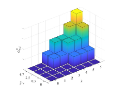
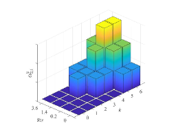
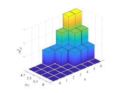
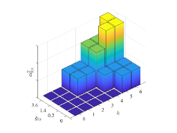
$\bullet$ Effect of policy on transmit powers of sensors: To show how transmit power $\alpha_{n,t}^{2}$ of sensor $n$ changes based on the adopted policy, we consider $N\!=\!2$ sensors. Recall for the sub-optimal policy $\alpha_{n,t}$ depends on the local state $s_{n,t}\!=\!(b_{n,t},\bar{g}_{n,t-1},e_{n,t-1})$, whereas for the optimal policy the local action $\alpha_{n,t}$ depends on the global state ${\boldsymbol{s}}_{t}\!=\!(s_{1,t},s_{2,t})$. We use Algorithm 1 and Algorithm 2, to find and set transmit power $\alpha^{2}_{n,t}$ corresponding to the optimal and the sub-optimal policies, respectively. Fig. 5 illustrates $(\alpha_{1,t}^{2},\alpha_{2,t}^{2})$ when optimal and sub-optimal policies are adopted, given a set of energy harvesting, battery-related, and channel-related parameters, and assuming the quantization thresholds are obtained via MMAE. To enable the illustration, we assume the state of energy harvesting for both sensors is “Fair”, i.e., $(e_{1,t-1},e_{2,t-1})\!=\!(2b_{u},2b_{u})$, and the states of battery $(b_{1,t},b_{2,t})$ and the states of quantized channel gains $(\bar{g}_{1,t-1},\bar{g}_{2,t-1})$ are variable. For example, this figure shows that when the local states are $s_{1,t}\!=\!(7,3,2),s_{2,t}\!=\!(7,3,2)$, then transmit powers of sensors corresponding to the optimal policy is $(\alpha_{1,t},\alpha_{2,t})\!=\!(1.5\mbox{mW},2\mbox{mW})$, whereas transmit powers of sensors corresponding to the sub-optimal policy is $(\alpha_{1,t},\alpha_{2,t})\!=\!(1\mbox{mW},3\mbox{mW})$. The Achievable $J_{tot}$ corresponding to optimal and sub-optimal policies are 11.58 and 10.43, respectively. These figures also show that, $\alpha^{2}_{n,t}(b_{n,t},\bar{g}_{n,t-1},e_{n,t-1})$ is monotonically increasing in $b_{n,t}$, given $\bar{g}_{n,t-1}$ and $e_{n,t-1}$.

Figure 6: The average $J$-divergence versus $b_{u}$ for $K\!=\!5,N\!=\!3,\mathcal{P}_{tot}\!=\!5$mW$,\gamma_{g}\!=\!2,L\!=\!3$, SNR${}_{s}\!=\!3$dB.

Figure 7: The average $J$-divergence versus SNR_s dB for $K\!=\!5,~{}N\!=\!3,\mathcal{P}_{tot}\!=\!5$mW$,b_{u}\!=\!1\mbox{mJ},\gamma_{g}\!=\!2,L\!=\!3.$

Figure 8: $P_{e}$ versus $\mathcal{P}_{tot}$ for $K\!=\!5,~{}N\!=\!3,~{}b_{u}\!=\!1\mbox{mJ},~{}\gamma_{g}\!=\!2,~{}L\!=\!3$,  SNR${}_{s}\!=\!3$dB.

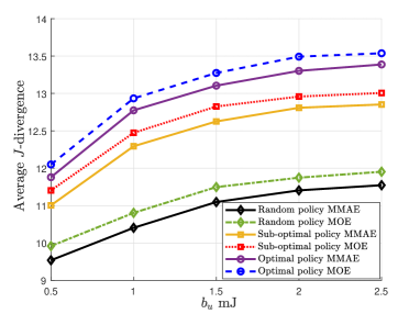
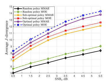
$\bullet$ Achievable $J$-divergence corresponding to optimal, sub-optimal, and random policies: Fig. 6 and Fig. 7 show average $J$-divergence versus $b_{u}$ and SNR_s respectfully. To plot the curves we set transmit power $\alpha^{2}_{n,t}$ corresponding to the optimal, the sub-optimal, and random policies, and then we average $J_{tot,t}\!=\!\sum_{n=1}^{N}J_{n,t}$ over $10^{4}$ independent Monte Carlo runs. For random policy, we randomly choose $\alpha^{2}_{n,t}$ such that the two constraints in (III) are satisfied, i.e., (i) $\alpha^{2}_{n,t}T_{s}/b_{u}\leq b_{n,t},~{}\forall t,n$, (ii) $\sum^{N}_{n=1}\alpha_{n,t}^{2}\leq{\cal P}_{tot},~{}\forall t$. Fig. 6 illustrates that, given a $K$ value, the average $J$-divergence increases in $b_{u}$, however, it remains almost the same after $b_{u}$ reaches and exceeds a certain value. This is due to the fact that, for larger $b_{u}$ values transmit power is not limited by energy harvesting and stored energy. Instead, it is limited by the communication channel noise variance $\sigma_{w}^{2}$. Fig. 7 shows that the average $J$-divergence increases in SNR_s. This is due to the fact that as SNR_s increases, $P_{f_{n}}=P_{f},\forall n$ in (II-A) decreases (given a $P_{d}$ value). Decreasing $P_{f}$ leads into increasing the average $J$-divergence, where $P_{f}$ and $J_{n,t}$ are related through (21) and (II-D). In both figures, average $J$-divergence achieved by the sub-optimal policy is smaller than average $J$-divergence achieved by the optimal policy, and larger than average $J$-divergence achieved by the random policy.

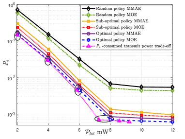
$\bullet$ $P_{e}$ corresponding to optimal and sub-optimal policies, and $P_{e}$-consumed transmit power trade-off: Fig. 8 shows $P_{e}$ versus ${\cal P}_{tot}$. To plot the curves we set transmit power $\alpha^{2}_{n,t}$ corresponding to the optimal and the sub-optimal policies, and then we consider $10^{4}$ independent Monte Carlo runs to find $P_{e}$, i.e., we generate $10^{4}$ realizations of random noises and fading channels and count the errors, $P_{e}$ is the number of errors occurred divided by $10^{4}$. Fig. 8 reveals two important points: (i) “optimal policy MOE” and “optimal policy MMAE” achieve the lowest $P_{e}$, followed by “sub-optimal policy MOE” and “sub-optimal policy MMAE”, followed by “random policy MOE” and “random policy MMAE”, (ii) “sub-optimal policy” performs very close to “optimal policy”. Note that for all curves, $P_{e}$ decreases as ${\cal P}_{tot}$ increases, however, it reaches an error floor after ${\cal P}_{tot}$ exceeds a certain value. This is due to the fact that for larger ${\cal P}_{tot}$ values, $P_{e}$ is not limited by ${\cal P}_{tot}$. Instead, it is limited by $\sigma_{w}^{2}$. Fig. 8 also allows us to examine the existing trade-off between the consumed transmit power and $P_{e}$. Consider the curve labeled “$P_{e}$-consumed transmit power trade-off” in Fig. 8, which shows how much transmit power is required to provide a certain $P_{e}$ value. This curve is obtained from examining the points on “optimal policy MOE” and checking whether the constraint $\sum^{N}_{n=1}\alpha_{n,t}^{2}\leq{\cal P}_{tot},~{}\forall t$. is active or inactive. At a given point, when this constraint is active (inactive), the consumed transmit power is equal to (less than) ${\cal P}_{tot}$. Note that as ${\cal P}_{tot}$ increases and $P_{e}$ reaches an error floor, the consumed transmit power is less than ${\cal P}_{tot}$.

Since finding the sub-optimal policy has a much lower computational complexity than that of the optimal policy, and its performance is very close to the optimal policy, from this point forward, we focus on the sub-optimal policy.

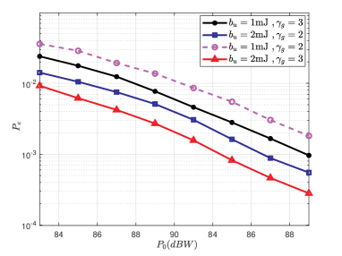
$\bullet$ Dependency of $P_{e}$ on different system parameters: Fig. 9-12 plot $P_{e}$ corresponding to sub-optimal policy in terms of different system parameters. Fig. 9 depicts $P_{e}$ versus $K$ as $\gamma_{g}$ and $b_{u}$ change. Given the pair ($\gamma_{g},b_{u}$), $P_{e}$ decreases as $K$ increases, until it reaches an error floor. The error floor becomes smaller as (i) $\gamma_{g}$ increases, given $b_{u}$, (ii) $b_{u}$ increases, given $\gamma_{g}$. The presence of error floor is due to the fact that, for larger $K$ values $P_{e}$ is no longer restricted by $K$, and instead it is restricted by $\sigma^{2}_{w}$, leading to an error floor.

Fig. 10 depicts $P_{e}$ versus $N$ as $f_{D}T_{s}$ and $P_{\text{d}}$ vary. We observe that, given the pair ($f_{D}T_{s},P_{\text{d}}$), $P_{e}$ reduces when $N$ increases, however, it reaches an error floor after cretin value of $N$. This is due to the fact that for larger $N$ values, $P_{e}$ becomes limited by ${\cal P}_{tot}$ and $\sigma_{w}^{2}$. Furthermore, we notice that $P_{e}$ decreases when (i) given the pair ($N$, $P_{\text{d}}$), $f_{D}T_{s}$ increases; (ii) given the pair ($N$, $f_{D}T_{s}$), $P_{\text{d}}$ increases.

Fig. 11 shows $P_{e}$ versus SNR_s as $L,N$ change. Examination of this figure shows that $P_{e}$ reduces when (i) given the pair ($L,N$), SNR_s increases. This is because as SNR_s increases, $P_{f_{n}}=P_{f},\forall n$ in (II-A) decreases, (ii) given the pair (SNR_s, $L$), $N$ increases, (iii) given the pair (SNR_s, $N$), $L$ increases. This is because as $L$ increases the feedback information from the FC to the sensors on channel gain increases.

Figure 9: $P_{e}$ vs. $K$ for $N\!=\!10,\mathcal{P}_{tot}\!=\!15$mW, $L\!=\!4,$ SNR${}_{s}\!=\!5$dB.

Figure 10: $P_{e}$ vs. $N$ for $K\!=\!10,\mathcal{P}_{tot}\!=\!15$mW, $b_{u}\!=\!2$mJ $\gamma_{g}\!=\!1.5,L\!=\!4,$ SNR${}_{s}\!=\!3$dB.

Figure 11: $P_{e}$ vs. SNR_s for $K\!=\!10,\mathcal{P}_{tot}\!=\!15$mW, $b_{u}=2$mJ, $\gamma_{g}\!=\!2$.

Figure 12: $P_{e}$ vs. $\eta$ for $K\!=\!10,N=5,\mathcal{P}_{tot}\!=\!15\mbox{mW},b_{u}\!=\!1,L\!=\!4,$SNR${}_{s}=3$dB.

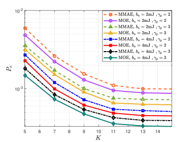
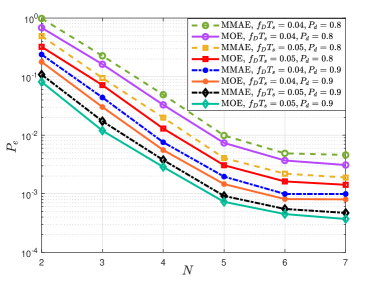
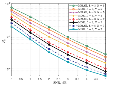
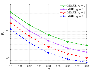
Fig. 12 shows $P_{e}$ versus $\eta$ as $\gamma_{g}$ varies. Given $\gamma_{g}$, $P_{e}$ decreases in $\eta$. This is due to the fact that, as $\eta$ increases, the sub-optimal $\alpha^{2}_{n,t}$ values increases, leading to a decrease in $P_{e}$. We note that there is a performance-computational complexity trade-off as $\eta$ increases. Recall the mean of the network lifetime $T$ is $\mathbb{E}\{T\}\!=\!1/(1-\eta)$. As $\eta$ increases, the number of iterations required for the value iteration algorithm (i.e., step 3 of Algorithm 2) to converge increases.

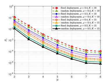
$\bullet$ Effect of random deployment of sensors on $P_{e}$: We consider a circle field where the signal source with power $P_{0}$ is located at its center. Sensors are randomly deployed in the field such that the distance of sensor $n$ from the source, $r_{n}$, is uniformly distributed in the interval of $(r_{0},r_{1})\!=\!(1\mbox{m},100\mbox{m})$. We assume the quantization thresholds are obtained via MMAE. Fig. 13 illustrates $P_{e}$ versus $P_{0}$ as $\gamma_{g}$ and $b_{u}$ change. We observe that $P_{e}$ decreases when: (i) given the pair ($\gamma_{g},b_{u}$), $P_{0}$ increases, (ii) given the pair ($P_{0}$, $b_{u}$), $\gamma_{g}$ increases, (iii) given the pair $(P_{0}$, $\gamma_{g}$), $b_{u}$ increases. These observations are all expected.

Fig. 14 illustrates $P_{e}$ versus $N$ for fixed and random deployment, as $\rho$ and $K$ vary. For the given set of parameters, the performance of fixed and random deployments is close to each other. Also, given the pair ($\rho,K$), $P_{e}$ reduces when $N$ increases, however, it reaches an error floor after $N$ exceeds a certain value. This is due to the fact that for larger $N$ values, $P_{e}$ becomes limited by ${\cal P}_{tot}$ and $\sigma_{w}^{2}$. Furthermore, we notice that $P_{e}$ decreases when (i) given the pair ($N$, $K$), $\rho$ increases, (ii) given the pair ($N$, $\rho$), $K$ increases.

Figure 13: $P_{e}$ vs. $P_{0}$ for $K\!=\!10,N\!=\!5,\mathcal{P}_{tot}\!=\!15$mW$,L\!=\!4,(r_{0},r_{1})\!=\!(1$m,$100$m).

Figure 14: $P_{e}$ vs. $N$ for $\mathcal{P}_{tot}\!=\!15\mbox{mW},b_{u}\!=\!4\mbox{mJ},\gamma_{g}\!=\!1.5,L=4$ (i) for fixed deployment SNR${}_{s}\!=\!5$dB, $P_{\text{d}}\!=\!0.9$, (ii) for random deployment $(r_{0},r_{1})\!=\!(1$m,$100$m), $P_{0}\!=\!84$dBW.

VI Conclusions

Considering an EH-enabled WSN with $N$ sensors and a feedback channel from the FC to the sensors, tasked with binary distributed detection, we developed adaptive channel-dependent transmit power control policies such that the detection performance is optimized, subject to total transmit power constraint. Modeling the quantized fading channel, the energy arrival, and the dynamics of the battery as homogeneous FSMCs, and the network lifetime as a random variable with geometric distribution, we formulated our power control optimization problem as a discounted infinite-horizon constrained MDP problem, where sensors’ transmit powers are functions of the battery state, quantized CSI, and the arrived energy. We developed the optimal policy, using dynamic programming and utilizing the Lagrangian approach to transform the constrained MDP problem into an equivalent unconstrained MDP problem. Determining the optimal policy, however, requires the knowledge of the global state at the FC, which imposes a significant signaling overhead to the sensors. To eliminate this overhead, we developed the sub-optimal policy, using a uniform Lagrangian multiplier to transform the constrained MDP problem into $N$ unconstrained MDP problems. Different from the optimal policy, in the sub-optimal policy each sensor sets its transmit power based on its local state information. We showed that the computational complexity of finding the sub-optimal policy scales linearly in $N$ and this policy has a close-to-optimal performance. We studies the error probability $P_{e}$ in terms of different system parameters, including $K,N,{\cal P}_{tot}$, SNR_s. Although $P_{e}$ decreases as each of these parameters increases, there is an error floor that ultimately depends on the communication channel noise variance and ${\cal P}_{tot}$. We expanded our work to random deployment of sensors and examined how it affects the error probability. The insights obtained in this work are useful for adaptive transmit power control of EH-enabled WSNs tasked with distributed detection.

References

- [1] D. Ciuonzo, P. S. Rossi, and P. K. Varshney, “Distributed detection in wireless sensor networks under multiplicative fading via generalized score tests,” IEEE Internet of Things Journal, vol. 8, no. 11, pp. 9059–9071, 2021.
- [2] H. R. Ahmadi and A. Vosoughi, “Distributed detection with adaptive topology and nonideal communication channels,” IEEE transactions on signal processing, vol. 59, no. 6, pp. 2857–2874, 2011.
- [3] Y.-W. Kuo, C.-L. Li, J.-H. Jhang, and S. Lin, “Design of a wireless sensor network-based iot platform for wide area and heterogeneous applications,” IEEE Sensors Journal, vol. 18, no. 12, pp. 5187–5197, 2018.
- [4] M. A. Al-Jarrah, M. A. Yaseen, A. Al-Dweik, O. A. Dobre, and E. Alsusa, “Decision fusion for IoT-based wireless sensor networks,” IEEE Internet of Things Journal, vol. 7, no. 2, pp. 1313–1326, 2019.
- [5] P. K. Varshney, “Distributed detection and data fusion,” 1996.
- [6] J. N. Tsitsiklis, “Decentralized detection by a large number of sensors,” Mathematics of Control, Signals and Systems, vol. 1, no. 2, pp. 167–182, 1988.
- [7] R. Viswanathan and P. K. Varshney, “Distributed detection with multiple sensors part i. fundamentals,” Proceedings of the IEEE, vol. 85, no. 1, pp. 54–63, 1997.
- [8] B. Chen, L. Tong, and P. K. Varshney, “Channel-aware distributed detection in wireless sensor networks,” IEEE Signal Processing Magazine, vol. 23, no. 4, pp. 16–26, 2006.
- [9] R. Niu, B. Chen, and P. K. Varshney, “Fusion of decisions transmitted over rayleigh fading channels in wireless sensor networks,” IEEE Transactions on signal processing, vol. 54, no. 3, pp. 1018–1027, 2006.
- [10] Z. Hajibabaei, A. Vosoughi, and N. Mastronarde, “Optimal power allocation for M-ary distributed detection in the presence of channel uncertainty,” Signal Processing, vol. 169, p. 107400, 2020.
- [11] H. R. Ahmadi and A. Vosoughi, “Impact of channel estimation error on decentralized detection in bandwidth constrained wireless sensor networks,” in MILCOM 2008-2008 IEEE Military Communications Conference. IEEE, 2008, pp. 1–7.
- [12] X. Zhang, H. V. Poor, and M. Chiang, “Optimal power allocation for distributed detection over mimo channels in wireless sensor networks,” IEEE Transactions on Signal Processing, vol. 56, no. 9, pp. 4124–4140, Sep. 2008.
- [13] H.-s. Kim and N. A. Goodman, “Power control strategy for distributed multiple-hypothesis detection,” IEEE Transactions on Signal Processing, vol. 58, no. 7, pp. 3751–3764, 2010.
- [14] H. R. Ahmadi, N. Maleki, and A. Vosoughi, “On power allocation for distributed detection with correlated observations and linear fusion,” IEEE Transactions on Vehicular Technology, vol. 67, no. 9, pp. 8396–8410, 2018.
- [15] N. Maleki and A. Vosoughi, “On bandwidth constrained distributed detection of a known signal in correlated gaussian noise,” IEEE Transactions on Vehicular Technology, 2020.
- [16] V. W. Cheng and T.-Y. Wang, “Performance analysis of distributed decision fusion using a censoring scheme in wireless sensor networks,” IEEE Transactions on Vehicular Technology, vol. 59, no. 6, pp. 2845–2851, 2010.
- [17] Z. Wang, V. Aggarwal, and X. Wang, “Iterative dynamic water-filling for fading multiple-access channels with energy harvesting,” IEEE Journal on Selected Areas in Communications, vol. 33, no. 3, pp. 382–395, 2015.
- [18] M.-L. Ku, W. Li, Y. Chen, and K. R. Liu, “Advances in energy harvesting communications: Past, present, and future challenges,” IEEE Communications Surveys & Tutorials, vol. 18, no. 2, pp. 1384–1412, 2015.
- [19] H. Yazdani and A. Vosoughi, “Steady-state rate-optimal power adaptation in energy harvesting opportunistic cognitive radios with spectrum sensing and channel estimation errors,” IEEE Transactions on Green Communications and Networking, 2021.
- [20] M. Nourian, S. Dey, and A. Ahlén, “Distortion minimization in multi-sensor estimation with energy harvesting,” IEEE Journal on Selected Areas in Communications, vol. 33, no. 3, pp. 524–539, 2015.
- [21] J. Geng and L. Lai, “Non-bayesian quickest change detection with stochastic sample right constraints,” IEEE Transactions on Signal Processing, vol. 61, no. 20, pp. 5090–5102, 2013.
- [22] S. S. Gupta, S. K. Pallapothu, and N. B. Mehta, “Ordered transmissions for energy-efficient detection in energy harvesting wireless sensor networks,” IEEE Transactions on Communications, vol. 68, no. 4, pp. 2525–2537, 2020.
- [23] A. Tarighati, J. Gross, and J. Jaldén, “Decentralized hypothesis testing in energy harvesting wireless sensor networks,” IEEE Transactions on Signal Processing, vol. 65, no. 18, pp. 4862–4873, Sep. 2017.
- [24] Q. Duan, X. Liu, and H. Wang, “Adaptive transmission control strategy for distributed detection in EH-WSNs,” in 2022 7th International Conference on Intelligent Computing and Signal Processing (ICSP), 2022, pp. 571–575.
- [25] G. Ardeshiri, H. Yazdani, and A. Vosoughi, “Optimal local thresholds for distributed detection in energy harvesting wireless sensor networks,” in 2018 IEEE Global Conference on Signal and Information Processing (GlobalSIP), Nov 2018, pp. 813–817.
- [26] G. Ardeshiri, H. Yazdani, and A. Vosoughi, “Power adaptation for distributed detection in energy harvesting wsns with finite-capacity battery,” in 2019 IEEE Global Communications Conference (GLOBECOM). IEEE, 2019, pp. 1–6.
- [27] G. Ardeshiri and A. Vosoughi, “On adaptive transmission for distributed detection in energy harvesting wireless sensor networks with limited fusion center feedback,” IEEE Transactions on Green Communications and Networking, vol. 6, no. 3, pp. 1764–1779, 2022.
- [28] O. Ozel, K. Tutuncuoglu, J. Yang, S. Ulukus, and A. Yener, “Transmission with energy harvesting nodes in fading wireless channels: Optimal policies,” IEEE Journal on Selected Areas in Communications, vol. 29, no. 8, pp. 1732–1743, Sep. 2011.
- [29] T. Banerjee, P. Gurram, and G. T. Whipps, “A bayesian theory of change detection in statistically periodic random processes,” IEEE Transactions on Information Theory, vol. 67, no. 4, pp. 2562–2580, 2021.
- [30] K. Premkumar and A. Kumar, “Optimal sleep-wake scheduling for quickest intrusion detection using wireless sensor networks,” in IEEE INFOCOM 2008-The 27th Conference on Computer Communications. IEEE, 2008, pp. 1400–1408.
- [31] X. Guo, Y. He, S. Atapattu, S. Dey, and J. S. Evans, “Power allocation for distributed detection systems in wireless sensor networks with limited fusion center feedback,” IEEE Transactions on Communications, vol. 66, no. 10, pp. 4753–4766, Oct 2018.
- [32] S. Mao, M. H. Cheung, and V. W. S. Wong, “Joint energy allocation for sensing and transmission in rechargeable wireless sensor networks,” IEEE Transactions on Vehicular Technology, vol. 63, no. 6, pp. 2862–2875, July 2014.
- [33] M. Ku, Y. Chen, and K. J. R. Liu, “Data-driven stochastic models and policies for energy harvesting sensor communications,” IEEE Journal on Selected Areas in Communications, vol. 33, no. 8, pp. 1505–1520, Aug 2015.
- [34] F. Zhang, T. Jing, Y. Huo, and K. Jiang, “Joint Optimization of Spectrum Sensing and Transmit Power in Energy Harvesting Cognitive Radio Sensor Networks,” The Computer Journal, vol. 62, no. 2, pp. 215–230, 02 2019.
- [35] M. L. Puterman, Markov decision processes: discrete stochastic dynamic programming. John Wiley & Sons, 2014.
- [36] M. Moghadari, E. Hossain, and L. B. Le, “Delay-optimal distributed scheduling in multi-user multi-relay cellular wireless networks,” IEEE Transactions on Communications, vol. 61, no. 4, pp. 1349–1360, April 2013.
- [37] F. Fu and M. V. Der Schaar, “A systematic framework for dynamically optimizing multi-user wireless video transmission,” IEEE Journal on Selected Areas in Communications, vol. 28, no. 3, pp. 308–320, April 2010.
- [38] D. Bertsekas, Dynamic programming and optimal control: Volume I. Athena scientific, 2012, vol. 1.
- [39] D. G. Luenberger and Y. Ye, Linear and nonlinear programming, 4th ed. Springer, 2015.
- [40] N. Maleki, A. Vosoughi, and N. Rahnavard, “Distributed binary detection over fading channels: Cooperative and parallel architectures,” IEEE Transactions on Vehicular Technology, vol. 65, no. 9, pp. 7090–7109, 2015.
- [41] R. Niu and P. K. Varshney, “Target location estimation in sensor networks with quantized data,” IEEE Transactions on Signal Processing, vol. 54, no. 12, pp. 4519–4528, 2006.