EarthNets: Empowering AI in Earth Observation

Abstract

Earth observation, aiming at monitoring the state of planet Earth using remote sensing data, is critical for improving our daily lives and living environment. With a growing number of satellites in orbit, an increasing number of datasets with diverse sensors and research domains are being published to facilitate the research of the remote sensing community. In this paper, we present a comprehensive review of more than 400 publicly published datasets, including applications like land use/cover, change/disaster monitoring, scene understanding, agriculture, climate change, and weather forecasting. We systematically analyze these Earth observation datasets with respect to five aspects volume, bibliometric analysis, resolution distributions, research domains, and the correlation between datasets. Based on the dataset attributes, we propose to measure, rank, and select datasets to build a new benchmark for model evaluation. Furthermore, a new platform for Earth observation, termed EarthNets, is released as a means of achieving a fair and consistent evaluation of deep learning methods on remote sensing data. EarthNets supports standard dataset libraries and cutting-edge deep learning models to bridge the gap between the remote sensing and machine learning communities. Based on this platform, extensive deep learning methods are evaluated on the new benchmark. The insightful results are beneficial to future research. The platform and dataset collections are publicly available at https://earthnets.github.io/.

1 Introduction

Earth Observation (EO) aims to monitor and assess the status of the Earth’s surface using various remote sensing (RS) technologies [1, 2]. EO can make a significant contribution to our ability to better understand and analyze the planet Earth using RS data. The research in EO has been successfully applied to urban planning[3], natural resources management[4], agriculture[5], food security [6] and disaster monitoring [7, 8]. All these applications are important for the sustainable development of human society.

With the development of Earth observation technology, more and more satellites with diverse imaging sensors have been launched for different missions. A huge amount of RS data with global coverage and high resolution is received every day for automatic processing and analysis. To deal with large-scale data, deep learning techniques [9] have been proven effective for many different research areas. In this context, recent RS datasets are constructed with larger and larger volumes of data. In Fig. 1, we show a chronological overview of the volumes of more than 400 existing benchmark datasets. As seen from this figure, more numerous and larger datasets have been constructed and published during the past decade. Although considerable progress has been made with the overwhelming success of deep learning techniques [10, 11], there are still several problems that need more research efforts to handle.

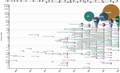
Figure 1: Chronological overview of the volumes of existing 400 datasets. As can be seen, more and more numerous and larger datasets have been constructed and published during the past decade. (Best viewed by zooming in.)

There is a lack of comprehensive dataset review for EO tasks. Owing to the efforts made by EO researchers, there are numerous datasets in the RS community with different modalities, resolutions, and application domains. Some of these RS data modalities include optical (RGB), hyperspectral, synthetic aperture radar (SAR), multi-spectral (MS), and point cloud. Regarding the application domains, the published datasets may be designed for land use and land cover (LULC) [12], change monitoring[13], disaster monitoring[14], scene recognition, semantic segmentation, ground object detection, object tracking, agriculture, climate change, and weather forecasting. A comprehensive review of the RS datasets can provide researchers with a holistic view of the status of the research community. Bakula et al. [15] review benchmarking in photogrammetry and remote sensing relating to geodata. They provide dataset collections and a bibliographic analysis, which are both useful for future research. Schmitt et al. [16] provide a historic review of RS datasets. They discuss dataset features based on a few examples and present some important criteria for the establishment of a standard database. Although a few works [17, 18, 19] attempt to review existing RS datasets, they are not exhaustive or sufficiently comprehensive to cover a large range of research domains.

There is no systematic summary and analysis of RS datasets. The ever-growing quantity of RS datasets makes it difficult to find the proper one for a specific application in the jungle of remote sensing datasets. For example, there are more than 20 datasets related to building extraction [20]. Finding, assessing, and selecting the one most suitable for a given application can be laborious and time-consuming. Thus, it is vitally important to summarize and categorize RS datasets to provide valuable guidance and reference for researchers. Both the EOD [21] and the AiTLAS Semantic Data Catalog have been designed as search engines for RS datasets, and are valuable and helpful for the RS community. However, at present, the information about RS datasets collected in these existing databases is still limited. Beyond summarization and categorization, insightful analysis of existing datasets can help researchers understand the current research state and trends of the whole community. Systematic analysis of RS datasets is thus crucial to the future development of different research fields.

There is no unified benchmark for fair comparisons of remote sensing methods. In the computer vision (CV) community, a large-scale dataset like ImageNet[22] is usually used for the evaluation of newly developed deep learning models. Compared with small-scale datasets, large-scale datasets with rich semantic annotations align better with complex real-world scenarios [17]. Thus they can be more reliable for performance validation and comparison of deep learning algorithms. Although several large-volume RS datasets have been published [23, 24, 25], many of the currently developed methods are still evaluated on small-scale datasets. However, datasets with a small scale or limited geographic coverage may bias to a specific data distribution that is not representative of real-world scenarios. Moreover, many RS datasets are published with no standard train/validation/test splits. This increases uncertainty during the evaluation of algorithms. Thus, building new RS benchmarks to enable a fair comparison of different methods is urgently needed.

At present, there is a lack of an open platform for different EO tasks. For deep learning methods, backbone networks, hyper-parameters, and training tricks are influential factors that should be considered for fair performance comparison. However, existing works usually evaluate the performance with different dataset splits, which makes it difficult to fairly and reliably compare different algorithms. Due to the large variance in data collection sensors and pre-processing pipelines, it is non-trivial to adapt modern deep learning models to RS datasets [26]. As a result, many cutting-edge and off-the-shelf deep learning methods from the machine learning community are not evaluated and compared on RS data. To address the aforementioned problems, in this study, we first make an exhaustive and comprehensive review of the publicly accessible RS datasets. Next, a systematic analysis is undertaken based on the information about these datasets. Based on the attribute information, we filter, rank, and select five large-scale datasets designed for general purposes in order to build a new benchmark for model evaluation. To further enable a fair and reproducible comparison of different algorithms, we construct a new deep learning platform, termed EarthNets, as a foundation for future work. Our main contributions are summarized below.

1. We review more than 400 datasets published in the RS community. These datasets are summarized and categorized into different research tasks and research domains. Detailed attributes including ten different aspects are provided for each dataset.

2. Systematic analyses are made with respect to five aspects of these datasets to provide insights and ideas for future research within the RS community. Specifically, the volume, bibliometric analysis, resolution distributions, research domains, and dataset relationship are considered for a comprehensive dataset analysis.

3. To our knowledge, we are the first to measure and rank existing RS datasets using the dataset attributes provided in this study. Based on this ranking and selection, a new benchmark is built for the evaluation of RS methods.

4. We analyze the relationships between different datasets. The dataset correlation matrix provides a new perspective to the RS community for the exploration of new algorithms across different datasets.

5. We release an open platform, termed EarthNets, for EO tasks. EarthNets aims to enable fair comparisons, efficient development of methods, and the greater availability of the RS data to a larger research community.

The rest of this paper is organized as follows. Section 2 reviews existing RS datasets for different tasks. Section 3 presents the analyses of the reviewed datasets from five different perspectives. Section 4 introduces the proposed dataset ranking and selection method, as well as the benchmark building process. Section 5 describes the newly released EarthNets platform. Section 6 presents the benchmarking results and analysis on the five selected RS datasets. Section 7 concludes the paper.

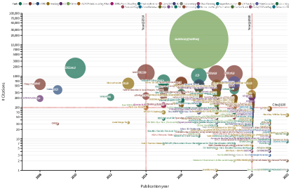
Figure 2: Chronological overview of the number of citations of existing RS datasets. UC Merd [27], AID [28] and DOTA [29] are the most cited works. (Best viewed by zooming in)

2 Remote Sensing Dataset Review

In this section, we review and organize more than 400 existing public RS datasets into five parts related to their tasks. Four of these tasks are common to many RS datasets: image classification, object detection, semantic segmentation, and change detection. For the purpose of an in-depth analysis of these datasets, we collect as much detailed information as possible for each dataset. Compared with existing review articles, our work provides richer information on the attributes of the datasets. Specifically, the following 10 aspects are considered.

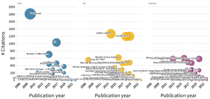
Figure 3: Visualization of the citation information of three different tasks. This figure shows that scene recognition and object detection datasets have more citations than segmentation datasets. However, object detection and semantic segmentation datasets attract more research attention after the year of 2019.

1) Research domain. In order to provide a clear presentation of these reviewed datasets, we organize them according to the specific domains in which they are created. Some typical research domains include agriculture, building, road, cloud, land use land cover (LULC), general scenes or objects, and so on.

2) Publication year. We provide the year of publication of the dataset, which is useful for the chronological analysis of these datasets.

3) Number of samples: To measure the dataset scale, we list the number of samples for each dataset. Note that it could be the number of images (for image-based datasets), the number of video clips (for video-based datasets), the number of points (for point cloud datasets), or the number of image pairs (for change detection datasets).

4) Size of sample: The size of each sample in the dataset is also an important factor for measuring the dataset scale. For images, the size is the height and width. For datasets designed for 3D understanding, the sample size could be the covered area.

5) Volume: The volume of each RS dataset is also factored in as a measurement of the dataset scale.

6) Number of Classes: For image classification, object detection, and semantic segmentation tasks, we provide the number of classes annotated in each dataset.

7) Data modality: For different EO tasks, a wide range of imaging sensors can be used to build datasets. For example, some of the data sources of RS datasets may include optical images, multi-spectral images, hyperspectral images [30], SAR[31], point cloud [32], and DSM (digital surface model)[33, 34].

8) Resolution range: The spatial resolutions of RS images have a high correlation with the image content. The resolution range is also highly relevant to specific EO tasks to which it can be applied.

9) Number of citations: We provide the number of citations for each dataset to measure its popularity in the RS community.

10) Dataset link: To facilitate the research, we provide the download link of each dataset. More detailed information can be found on https://earthnets.github.io/.

2.1 RS Image Classification Datasets

Image classification is a fundamental task in both the CV and RS communities. With image- or patch-level annotations, RS image classification has been employed in many different real-world applications. In Table I, 91 RS image classification datasets are reviewed and presented. In order to facilitate researchers to search and index, we organize them into different research domains. To be specific, Table I contains 13 agriculture-related datasets [35, 36, 37, 38]. For agriculture-related applications, the images or patches in the datasets are labeled with binary labels (crop/non-crop) or crop type labels (up to 348 granular labels). For general scene classification, 16 datasets are presented in the table. Million-AID the largest of these, contains a million instances for training and evaluation of scene classification methods. MLRSNet [39], RSD46-WHU [40], and NWPU-RESISC45 [41] are annotated with more than 40 class labels. There are 19 datasets for LULC applications in the table. Among these datasets, multiple types of data sources are used, including hyperspectral [30], multi-spectral [42, 23, 43, 44], SAR [45] and RGB data [46, 47].

There are 5 ship-related [48, 49, 50, 51] and 5 flood-related [52, 53, 54] datasets for RS image classification task. For the cloud-related research domain, 4 datasets are reviewed in this table. Some specific domains with fewer datasets are also presented, like smoke [55], sea lion [56], solar power plants [57] and wind datasets [58]. It is worth noting that species classification datasets are annotated with the most semantic labels.

Compared with object detection (with object-level annotation) and pixel-level segmentation tasks, agriculture-related applications are mainly modeled as image classification tasks. In contrast, aircraft [31] and ship-related datasets are built primarily for object detection tasks. For agriculture-related datasets, data from the Sentinel satellites is mostly used with a lower spatial resolution to cover larger crop areas. General scene classification and LULC are the two dominant domains in RS image classification datasets. From the bibliometric view, general scene classification and LULC datasets are cited much more often than other research domains. This indicates that scene classification is a heavily studied research direction in the RS community.

TABLE I: Detailed Information about 91 RS Image Classification Datasets. These datasets are grouped into 27 different research domains in alphabetical order. Note that / denotes the missing information; the number of citations are retrieved as of Sep. 2022. The download links for all these datasets can be found at https://earthnets.github.io.

Domain	Name	Year	#Samples	Sample Size	#Classes	Modailty	Resolution	Vol.(GB)	#Cita.
Agriculture	Brazilian Coffee Scene [35]	2015	2876	64	2	RGB	20m	0.004	703
	Indian Pines[59]	2015	1	145	16	Hyperspectral	20m	0.0059	/
	Salinas[30]	2015	1	365	16	Hyperspectral	3.7m	0.026	/
	Crop Type Mapping Ghana[60]	2019	/	/	18	Sentinel-1,Sentinel-2,Planet	3$\sim$10m	312.54	/
	CV4A Kenya[61]	2020	4688	2016x3035	7	Sentinel-2	10m	3.5	9
	BreizhCrops[62]	2020	610000	/	9	Sentinel-2,MT	10$\sim$60m	/	34
	CaneSat[63]	2020	1627	10	2	Sentinel-2,MT	10m	0.006	/
	CropHarvest[64]	2021	90,480	12 ts	343	Sentinel-1,Sentinel-2,ERA5,DEM	10$\sim$60m	20	5
	South Africa Crop Type[65]	2021	122736	/	9	Sentinel-1,Sentinel-2	/	82.77	/
	DENETHOR[36]	2021	/	/	9	Sentinel-1,Sentinel-2	3m	254.5	9
	The Canadian Cropland[38]	2022	78536	64	10	Sentinel-2	10m	26	0
	Space2Ground[66]	2022	10102	260	2	Sentinel-1,Sentinel-2,RGB	10$\sim$60m	0.501	0
	Sen4AgriNet[37]	2021	225000	366	158	Sentinel-2	10$\sim$60m	10240	1
Aircraft	SAR-ACD[31]	2022	4322	64	20	SAR	/	/	1
Cloud	SPARCS [67]	2016	80	1000	7	MS,Landsat	30m	1.43	168
	Kaggle Cloud Detection[68]	2019	9244	1750	4	RGB	/	5.86	0
	CloudCast[69]	2020	70080	1229	10	NWP	3km	320.31	6
	Sentinel-2 Cloud Mask Catalogue[70]	2020	513	1022	3	Sentinel-2	20m	15.38	/
Event	ERA[71]	2020	343680	640	25	RGB Video	/	6.3	12
Flood	Hurricane Damage[52]	2019	16000	128	2	RGB	1m	0.064	33
	SEN-12-FLOOD[53]	2020	336	512	2	RGB,SAR,MS	10m	12.2	14
	Sen1Floods11[54]	2020	4831	512	1	Sentinel-1	10m	14.3	40
	OMBRIA [72]	2022	3376	256	2	Sentinel-1,Sentinel-2	10m$\sim$20m	0.19	2
	FloodNet[14]	2021	2343	4000	9	RGB	0.015m	2.1	31
Forest	Kaggle Planet Forest[73]	2017	150000	256	17	RGB-NIR	5m	32.23	/
General Scenes	OVERHEAD MNIST[74]	2020	1000	28	9	Grayscale	/	0.017	35
	fMoW[24]	2018	523846	/	63	RGB,MS	0.3m	3500	146
	UC Merced[27]	2010	2100	256	21	RGB	0.3m	0.3	1808
	WHU-RS19[75]	2012	1013	600	19	RGB	0.5m	0.1	212
	RSSCN7[76]	2015	2800	400	7	RGB	/	0.086	441
	NWPU-RESISC45[41]	2016	31500	256	45	RGB	0.2$\sim$30m	0.404	176
	RSC11[77]	2016	1232	512	11	RGB	/	0.63	75
	AID[28]	2017	10000	600	30	RGB	3m	2.4	1028
	RSD46-WHU[40]	2017	117000	256	46	RGB	0.5$\sim$2m	11	460
	PatternNet[78]	2018	30,400	256	38	RGB	0.062$\sim$4.693m	1.3	260
	OPTIMAL-31[79]	2019	1860	256	31	RGB	/	0.024	373
	MLRSNet[39]	2020	109,161	256	46	RGB	0.1$\sim$10m	1.254	25
	CLRS[80]	2020	15000	256	25	RGB	0.26$\sim$8.85m	1.735	16
	Million AID[17]	2021	1,000,000	150$\sim$550	28	RGB	0.5$\sim$153m	133.5	29
	NaSC-TG2[81]	2021	20000	256	10	RGB-NIR	100m	/	8
	Satellite Image Classification [82]	2021	5631	256	4	RGB	/	0.023	/
Multi-label Scenes	MultiScene[83]	2021	100,000	512	36	RGB	0.3$\sim$0.6m	0.85	1
Geophysical	Hephaestus[84]	2022	216106	224	6	InSAR	/	93.71	0
Golf Course	MUSIC4GC (Golf Course)[85]	2017	83431	16	2	MS,Landsat	30m	0.37	12
Hot Area	MUSIC4HA (Hot Area)[85]	2022	2511	16	6	Sentinel-2	10m	0.01	1
Iceberg	Iceberg Detection[86]	2018	10028	75	2	SAR	/	0.295	/
Land Cover	SAT-4[87]	2015	500000	28	4	RGB-NIR	1$\sim$6m	7.25	43
	SAT-6[87]	2015	405000	28	6	RGB-NIR	1m	5.65	43
	Botswana [30]	2015	1	875	14	Hyperspectral	30m	0.077	/
	TiSeLaC[88]	2017	23	2866x2633	9	RGB-NIR,MT	30m	/	/
	Gaofen Image Dataset (GID)[89]	2018	150	7200	15	RGB-NIR	4m	71.1	274
	MSLCC[45]	2018	2	5596×6031,8149×5957	4	SAR,MS	10m	0.5	26
	BigEarthNet[42]	2019	590326	120	43	Sentinel-1,Sentinel-2	10m, 20m, 60m	121	203
	Slovenia Land Cover[90]	2019	940	500	10	Sentinel-2	10m	11.55	/
	So2Sat LCZ42[23]	2019	400673	32	17	Sentinel-1,Sentinel-2	10m	50.59	75
	TG1HRSSC [91]	2021	204	512	9	Hyperspectral	5m, 10m, 20m	0.277	4
Land Use	SIRI-WHU (Google+USGS)[46]	2016	2400	200	12	RGB	2m	0.7	288
	RSI-CB256[47]	2017	24000	256	35	RGB	0.3$\sim$3m	2.2	37
	RSI-CB128[47]	2017	36000	128	45	RGB	0.3$\sim$3m	0.88	37
	Austin Zoning[92]	2017	3,666	773x961	5	RGB	/	0.596	/
	HistAerial [93]	2019	42000	25,50,100	7	Grayscale	/	7.6	29
	AiRound[43]	2020	11753	300	11	RGB,Sentinel-2,Ground,Aerial	/	33	5
	CV-BrCT[43]	2020	24000	500	9	RGB	/	9.2	5
	EuroSAT[44]	2018	27000	64	10	Sentinel-2	10m	1.92	32
	SenseEarth classify [94]	2020	70000	100$\sim$12655	51	RGB	0.2$\sim$153m	10.8	/
Landslide	Bijie Landslide[95]	2020	2773	200	2	RGB	0.68m	0.51	84
Military	MSTAR-8class[96]	1996	9466	368	8	SAR	0.3m	0.444	/
Plant/Tree	Forest Cover Type[97]	2013	581012	12	7	Tree Attributes	/	0.07	/
	Pasadena Urban Trees	2016	100,000	/	18	RGB	/	/	161
	Aerial Cactus Identification[98]	2019	17000	32	2	RGB	/	0.025	/
	WiDS Datathon 2019[99]	2019	11000	256	2	RGB	3m	0.46	/
	The Auto Arborist Dataset[100]	2022	2,637,208	1,024	344	RGB,MS	/	24	1
	TreeSatAI[101]	2022	50381	304x304,6x6	47	Sentinel-1,Sentinel-2,RGB	10m,0.2m	16.3	0
	Forest Damages Larch Casebearer[102]	2021	1543	1500	5	RGB	UAV	3.3	/
Sea lion	NOAA Sea Lion Population Count[56]	2017	950	4900	4	RGB	/	96	13
Ship	Ships in Satellite Imagery[48]	2017	4000	80	2	RGB	3m	0.343	/
	MASATI[49]	2018	7389	512	7	RGB	0.08$\sim$2m	2.3	93
	DSCR[50]	2019	20,675	150$\sim$800	7	RGB	/	/	7
	FGSCR-42[50]	2021	9320	140$\sim$800	42	RGB	/	4.76	7
	SynthWakeSAR[51]	2022	46080	96000	10	SAR	3.3m	4.3	0
Smoke	USTC_SmokeRS [55]	2019	6225	256	6	RGB	1000m	0.79	49
Solar Power Plants	MUSIC4P3[57]	2017	1280000	16	2	MS,Landsat	30m	4.6	7
Species	GeoLifeCLEF 2021[103]	2021	19,000,000	256	31,435	RGB-IR,MS,LC,DEM	1m,0.3m,0.1m	840	19
Tailings Dam	BrazilDAM[104]	2020	769	384	2	RGB	10$\sim$60m	57	11
Urban Village	S2UC [105]	2021	1714	224	2	RGB	2m	1.8	1
Vegetation	Kennedy Space Center[106]	2015	1	550	13	Hyperspectral	0.18m	0.055	/
	Brazilian Cerrado-Savanna [107]	2016	1311	64	4	MS	5m	0.011	17
Vehicles	WAMI DIRSIG [108]	2017	55226	64	2	Hyperspectral	0.3m	0.33	48
	Kaggle Find a Car Park[109]	2019	3262	1296	2	RGB	/	2.75	/
	MAFAT-Fine-Grained [110]	2021	4216	/	37	RGB	0.05$\sim$ 0.15m	/	/
Wind	Airbus Wind Turbine Patches[58]	2021	155,000	128	2	RGB,MS	1.5m	1	/

2.2 RS Object Detection Datasets

Object detection has a close relationship with real-world applications like autonomous driving, video surveillance, and many other high-level scene understanding tasks. Thus, a number of widely-read works have been published in the CV community, like Faster RCNN [111], SSD [112], YOLO [113], and Transformer-based detectors [114]. For the RS object detection task, more and larger datasets are also being published for different EO applications, including aircraft detection [115, 116, 117], building detection [118, 119, 120, 121], ship detection [122, 123, 124, 125], vehicle detection [126, 127, 128, 129, 130], general ground object detection [131, 132, 133, 134, 135, 29] and other research domains [136, 137, 138].

In Table II, 91 RS object detection datasets are reviewed and organized into 18 different research domains. The most popular domains for RS object detection tasks are general object detection with 12 datasets, building detection with 12 datasets, aircraft detection with 8 datasets, ship detection with 14 datasets, and vehicle-related object detection with 20 datasets. Similar to RS image classification tasks, datasets for general object detection have higher citation numbers. Since object detection is a task with object-level annotations, the spatial resolutions of these datasets are usually higher than those of image classification datasets. However, for objects with large sizes, like ships, the data from Sentinel-1 and Sentinel-2 satellites are also used [139, 140]. For the detection of traffic objects [141] or other small objects [142], images captured from Unmanned Aerial Vehicles (UAV) are usually used.

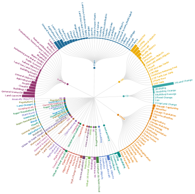
Figure 4: Research Domains (outer perimeter) Organized by EO Tasks (inner labels). It can be seen that there are strong correlations between research domain and EO tasks.

2.3 RS Semantic Segmentation Datasets

Pixel-level semantic segmentation aims to assign semantic labels to each pixel of the input image. Compared with image-level and object-level tasks, interpreting the image data with semantic maps can provide a more complete understanding of the scene. In Table III, we review and present 101 datasets for RS semantic segmentation tasks. Among them, 25 datasets are built for LULC or general scene segmentation tasks [143, 144, 145, 146, 147, 148, 33, 34, 25]. There are 18 additional datasets constructed for the segmentation of general scenes.

TABLE II: Detailed Information about 91 RS Object Detection Datasets. These datasets are grouped into 18 different research domains in alphabetical order. Note that / denotes the missing information; the number of citations are retrieved as of Sep. 2022. The download links for all these datasets can be found at https://earthnets.github.io.

Domain	Name	Year	# samples	Size	# classes	Modality	Resolution	Volume (GB)	# Citations
Agriculture	PASTIS [149]	2021	2433	128	18	Sentinel-2	10m	29	15
Aircraft	PlanesNet [115]	2017	32000	20	2	RGB	/	0.4	/
	MTARSI (Aircraft) [150]	2019	9385	256	2	RGB	/	0.48	/
	RarePlanes [151]	2020	713348	512	110	MS,WorldView3	0.3$\sim$1.5m	310.55	32
	CGI Planes [152]	2021	500	/	2	RGB	/	0.7	/
	CASIA-aircraft [117]	2021	58,121	399	2	RGB	/	/	/
	Airbus Aircraft Detection [116]	2021	109	2560	2	RGB	0.5m	0.092	/
	SAR Aircraft [153]	2022	2966	224	2	SAR	0.5m$\sim$3m	0.18	2
	Military Aircraft [154]	2022	3842	800	20	RGB	/	1.1	0
Bridge	Bridges Dataset [155]	2019	500	4800x2843	2	RGB	0.5m	1.45	6
Building	SpaceNet-4 (Multi-View) [121]	2018	60000	900	1	MS,WorldView2	0.3m	186	45
	DeepGlobe (Building) [118]	2018	24586	650	2	Panchromatic,RGB,MS	0.5m	/	470
	WHU Building [156]	2018	25577	512	2	RGB	0.3m	24.41	414
	CrowdAI Mapping [157]	2018	401,755	300	1	RGB	/	5.3	/
	Map Challenge [157]	2018	341,058	300	2	RGB	/	/	23
	TBF [158]	2018	13	40,000	2	RGB	/	/	/
	Microsoft Building (Australia) [159]	2019	11,334,866	/	2	/	/	6.4	/
	Microsoft Building (Uganda/Tanzania) [160]	2019	17,942,345	/	2	/	/	3.5	/
	Microsoft Building (USA) [119]	2019	129,591,852	/	2	/	/	34.4	/
	Microsoft Building (Canada) [161]	2019	11,842,186	/	2	/	/	2.5	/
	Urban Building Classification [162]	2022	800	600	61	RGB	0.5$\sim$0.8m	0.675	/
	BONAI [163]	2022	3,300	1,024	1	RGB	0.3m$\sim$0.6m	4.86	1
General	NWPU-VHR10 [131]	2014	800	1000	10	RGB,IRRG	0.08$\sim$2m	0.07	1264
	RSOD [132]	2017	976	1000	4	RGB	0.3$\sim$3m	0.077	460
	TGRS HRRSD [133]	2017	21761	10569	13	RGB	0.15$\sim$1.2 m	8.6	126
	xView [134]	2018	1,413	3,000	60	RGB,MS	0.3m	20	188
	fMoW [135]	2018	523846	/	63	RGB,MS	0.3m	3500	146
	DOTA v1.0 [29]	2018	2806	4000	15	RGB	/	18	1193
	DOTA v1.5 [164]	2019	2806	4000	16	RGB	/	18	1198
	DIOR [18]	2019	23463	800	20	RGB	0.5$\sim$30 m	6.93	481
	DOTA v2.0 [165]	2020	11268	4000	18	RGB	0.1$\sim$0.81	34.3	69
	iSAID [166]	2020	2806	4000	15	RGB	/	18	110
	VALID [167]	2020	6690	1024	30	RGBD	/	15.7	15
	UAVOD10 [136]	2022	844	1000$\sim$4800	10	RGB	0.15m	0.9	0
Human/Animals	BIRDSAI [168]	2020	162000	640	10	Thermal	UAV@60-120m	3.7	25
Land Covers	Dstl Satellite Imagery [137]	2017	57	3,348	10	RGB,MS	0.3m$\sim$7.5m	21.7	/
Object Counting	RSOC (Object Counting) [169]	2020	3057	2500	4	RGB	/	0.082	14
Oil Storage Tanks	Oil and Gas Tank (OGST) [170]	2020	10000	512	2	RGB	0.3m	1.87	/
	Airbus Oil Storage Detection [138]	2021	103	2560	2	MS	1.2m	0.102	/
	Oil Storage Tanks [171]	2019	10000	512	2	RGB	0.5m	3	/
Volcanoes	Hephaestus [172]	2022	216106	224	6	InSAR	/	93.71	0
Person	Semantic Drone-OD [173]	2019	400	5000	2	RGB	/	3.91	/
	Stanford Drone [174]	2016	100	1400x1904	6	RGB Video	0.025m	69	616
Sea	NOAA Sea Lion Count [56]	2017	950	4,900	4	RGB	/	96	13
	Aerial Maritime Drone [175]	2020	508	800x600	5	RGB	/	0.038	18
	SeaDronesSee [176]	2022	5630	3,840$\sim$5,456	6	RGB	/	60.3	9
	AFO-Floating objects [177]	2020	3647	720$\sim$3840	6	RGB	/	4.7	9
Search/Rescue	Search And Rescue [178]	2021	2552	1000	1	RGB	0.5m	/	3
Ship	OpenSARShip [122]	2017	11346	900	1	Sentinnel-1	10m	1.7	176
	SSDD [123]	2017	1160	500	2	SAR	1$\sim$15m	/	298
	HRSC2016 (Ship) [179]	2017	1061	300x300$\sim$1500x900	26	RGB	0.4$\sim$2m	3.74	203
	Kaggle Airbus Ship [124]	2018	192556	768	2	/	1.5m	31.41	/
	Airbus Ship Detection [124]	2018	40,000	768	2	RGB	/	31.4	/
	Ships in Google Earth [125]	2018	794	2000	2	RGB	/	2	/
	SAR Ship Detection [180]	2019	43819	256	2	SAR	3m, 5m, 8m,10m	0.4	204
	AIR-SARShip-1.0 [181]	2019	31	3000	2	SAR	1$\sim$3m	0.24	0
	AIR-SARShip-2.0 (GF-3) [148]	2020	300	1,000	2	SAR	1$\sim$3m	0.22	108
	LS-SSDD (Large Scale) [139]	2020	15	20,000	2	Sentinel-1,SAR	0.5,1,3m	7.8	69
	HRSID (Ship) [140]	2020	5,604	800	2	Sentinel-1,SAR	0.5$\sim$3m	0.58	128
	SWIM-Ship [182]	2021	14610	768	2	RGB	0.5$\sim$2.5m	12.5	0
	CASIA-Ship [183]	2021	1,118	1,680	2	RGB	/	/	/
	xView3-SAR [184]	2022	1000	$\sim$29400x24400	2	Sentinel-1	10m	1500	0
Small Objects	AI-TOD [141]	2021	28036	800	8	RGB	0.3m$\sim$30m	42	22
	SODA-A [142]	2022	2510	4761×2777	9	RGB	/	/	0
Traffic Objects	AU-AIR [185]	2020	32823	1920	8	RGB	UAV@30m	2.2	57
	HighD [186]	2018	110000	4096x2160	2	RGB	/	/	519
	Interaction Dataset [187]	2019	10,933	/	1	RGB	/	/	196
	Intersection Drone [188]	2020	11,500	4096x2160	5	RGB	/	/	120
	Roundabouts Drone [189]	2020	13,746	4096x2160	8	RGB	/	/	52
Tree	NEON Tree Crowns [190]	2020	11,000	100 million trees	2	RGB	/	27.4	3
	Forest Damages [191]	2021	1543	1500	5	RGB	UAV	3.3	/
Vehicles	Things And Stuff (TAS) [126]	2008	30	792	2	RGB	0.5m	0.01	550
	OIRDS [192]	2009	900	256$\sim$640	5	RGB	0.15m	0.153	30
	UCAS_AOD [193]	2014	976	1,000	2	RGB	/	3.24	232
	VEDAI(Vehicle) [127]	2015	1,250	1,024	9	IRGB	0.125m	3.9	350
	PKLot(Parking Lot) [194]	2015	12417	1280	2	RGB	UAV	4.6	236
	COWC [128]	2016	388435	256	2	RGB	0.15m	62.5	265
	Car Parking Lot (CARPK) [195]	2016	1448	1280	2	RGB	UAV	2	235
	DLR3k/DLR-MVDA [129]	2016	20	3744	7	RGB	0.13m	0.162	/
	ITCVD (Vehicle) [130]	2018	173	5616	2	RGB	0.1m	12	47
	VisDrone2019-DET [196]	2019	10209	2000x1500	10	RGB	UAV	2	48
	VisDrone2019-VID [196]	2019	40000	3840x2160	5	RGB	UAV	14	48
	VisDrone2019-SOT [196]	2019	139300	3840x2160	3	RGB Video	UAV	68	48
	VisDrone2019-MOT [196]	2019	40000	3840x2160	5	RGB Video	UAV	14	48
	SIMD (Multi-vehicles) [197]	2020	5000	1024	15	RGB	UAV@150m	1	6
	VisDrone [198]	2020	275,437	1,400	11	RGB	UAV	16	46
	EAGLE [199]	2020	8820	936	2	RGB	0.05$\sim$0.45m	/	16
	MOR-UAV [200]	2020	10948	1080	1	RGB	UAV	/	21
	DroneVehicle [201]	2021	56,878	840	5	RGB-Infrared	UAV@100m	13.09	4
	Swimming pool/car [202]	2019	3750	224	2	RGB	/	0.12	/
	ArtifiVe-Potsdam [203]	2021	4800	600	1	MS	0.05m	15.6	2

There are 13 datasets [157, 158, 159, 160, 119, 161, 162] that are designed for building extraction with pixel-level annotations. Note that some of them are constructed for building instance segmentation tasks. In those cases, the buildings are annotated with both the object-level and pixel-level labels. For road extraction, 9 datasets [204, 205, 19, 206, 207, 208, 209] are constructed. Datasets designed for LULC, general scenes, buildings, and road segmentation dominate the RS semantic segmentation tasks. For cloud-related applications, there 10 datasets built with lower spatial resolution RS images than other domains [210, 211, 212, 213, 214]. Furthermore, 9 agriculture datasets are annotated with pixel-level labels [215, 216, 217, 149, 218]. From the bibliometric view, building and road extraction are highly cited domains. This makes sense because building and road segmentation tasks are widely used in real-world applications.

2.4 RS Change Detection and Other Tasks

RS change detection aims to quantitatively analyze surface changes based on remotely-sensed data. It is a critical tool for real-world applications like damage monitoring and urban planning. In Table IV, we present 35 datasets that are built for RS change detection tasks. Most of them focus on the change of land cover or land use. Several other datasets are constructed for 3D change detection [219], building-specific change detection [220], and flood-related change detection [221]. Many different data modalities are used for constructing these datasets, including optical (RGB), point cloud, hyperspectral, multi-spectral, and SAR. Note that some datasets like SECOND [222] and Dynamic World [223] are annotated with pixel-wise semantic labels, not only the change/non-change binary label.

Apart from RS image classification, object detection, semantic segmentation and change detection tasks, we also list 83 datasets constructed for other tasks in the supplementary materials. For example, image captioning datasets [224, 225] and visual question answering datasets [226, 227] combine RS data with natural languages. Multi-view stereo datasets [228, 229, 230] are used for 3D reconstruction. There are also datasets used for more sporadic tasks like geo-localization [231, 232], weather forecasting [233, 234], oil parameter estimation [235], and wind speed estimation [58, 236].

3 Remote Sensing Dataset Analysis

In this section, we analyze the reviewed more than 400 RS datasets and provide statistics related to five different aspects of these datasets.

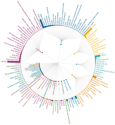
Figure 5: Data Modalities (outer perimeter) Organized by EO tasks (inner labels). Although there is a wide range of data sources used for EO, optical data (RGB) is still the most used modality for the majority of RS tasks.

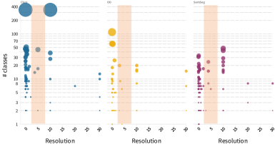
Figure 6: Visualization of The Relationships Between Data Resolution and The Number of Annotated Classes. An interesting finding is that most datasets have the resolution that is either smaller than 1m or larger than 10m. Datasets with resolution range of between 1 to 10m are obviously scarce.

3.1 The Volume Trend

Thanks to their powerful representation learning capabilities, deep learning networks trained with large-scale datasets have shown performance that is superior to that of classical machine learning methods. In the deep learning era, large-scale datasets play an important role in training deep models that yield better performance as well as better generalizability. Another advantage of large-scale datasets is that they align better with real-world scenarios. In Fig. 1, we visualize a chronological overview of the volume of 401 RS datasets. Note that the volume (in GBs) shown in this figure is transformed into the logarithmic scale, and larger circles indicate larger volumes. It can be clearly seen that datasets before the year 2015 are usually smaller in volume. Similar to the CV community, after deep learning became the mainstream technique, both the number and the volume of RS datasets significantly increase. For example, the volumes of fMoW [135] and Sen4AgriNet [37] are greater than 4000 GB. Well-annotated large scale datasets can greatly help the RS community in developing and evaluating more powerful deep learning models with better performance and generalizability.

3.2 Bibliometric Analysis

Citation information from 2008 to 2022 is shown in a chronological order in Fig. 2. The number of citations was collected as of Sep. 2022. From the figure it can be seen that the dataset with the highest number of citations is Aerial2map [237]. Aerial2map is a dataset for image translation, and the pixel2pixel algorithm is the reason for its high number of citations. In general, Fig. 2 shows that datasets published during the year range of 2014 to 2020 have a higher number of citations than those before or after.

UC Merced [27], AID [28] for scene classification, NWPU VHR10 [41], and DOTA [29, 164] for object detection are datasets with a particularly high number of citations. After the year of 2020, we can see that the VQA dataset [226] and SeCo dataset [238] for self-supervised learning have attracted increasing research attention in the RS community.

In Fig. 3, we display the citation information of three different tasks: the RS image classification, object detection, and semantic segmentation. From this figure we can clearly see that scene recognition and object detection datasets have more citations than segmentation datasets. However, there are more object detection and semantic segmentation datasets published after the year of 2019. This indicates that object-level and pixel-level understanding of RS images is becoming increasingly popular in the RS community.

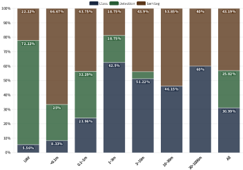
Figure 7: Visualization of the task distributions with regard to different spatial resolutions. Datasets with UAV images are mostly constructed for object detection. Datasets with the resolution range of 1m to 30m are mostly designed for image classification and semantic segmentation tasks.

3.3 Analysis of Data Modalities

To analyze the image sources used in the RS community, we summarize and visualize the data modalities used for different RS tasks. The relationships between data modalities and RS tasks are shown in Fig. 5. Although there is a wide range of image sources, optical data (RGB) is still the most frequently used modality for the majority of RS tasks. In Fig 4, we display the relationships between tasks and research domains.

3.4 Analysis of Spatial Resolutions

For RS images, spatial resolution has a high correlation to image content. In Fig. 6, we show the relationships between data resolution and the number of annotated classes. In general, this figure clearly shows that the number of semantic classes for RS image classification tasks is higher than for RS object detection and segmentation tasks. The reason is that object-level and pixel-level datasets require much more annotation efforts when the number of semantic classes increases.

Another interesting finding is that most datasets have a resolution of smaller than 1m or larger than 10m. The datasets with resolution in the range between 1 to 10m are obviously scarce. The reason for this phenomenon is that many EO applications require either high-resolution (<1m) imagery or global coverage (Sentinel 1&2, >10m). However, the EO data with resolution 1$\sim$10m also has great potential in a range of applications. More research attention should be devoted to filling in this gap.

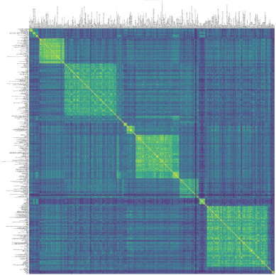
Figure 8: Visualization of the correlation between different datasets. Lighter color means higher correlation. For the first time, we propose to analyze the correlations between different RS datasets based on their attribute information collected in this study (Best viewed in color).

TABLE III: Detailed Information of 101 RS Semantic Segmentation Datasets. These datasets are grouped into 19 different research domains in alphabetical order. Note that  denotes the missing information; the number of citations are retrieved as of Sep. 2022. The download links for all these datasets can be found at https://earthnets.github.io.

Domain	Name	Year	#Samples	Sample Size	#Classes	Modailty	Resolution	Vol.(GB)	#Cita.
Agriculture	Agricultural Crop Cover[215]	2018	40	/	2	MS	30m	4.4	/
	GF2 Dataset for 3DFGC [216]	2019	11	2,652	5	RGB-NIR	4m	0.056	22
	TimeSen2Crop [217]	2020	1000000	10980	16	Sentinel-2	10m	1.1	11
	Agriculture-Vision [218]	2020	94986	512	9	RGB-NIR	0.1$\sim$0.2m	4.4	81
	WHU-Hi-LongKou [239]	2020	1	550x400	9	Hyperspectral	0.463m	/	2
	WHU-Hi-HanChuan [239]	2020	1	1217x303	16	Hyperspectral	0.109m	/	2
	WHU-Hi-HongHu [239]	2020	1	940x475	22	Hyperspectral	0.043m	/	2
	ZueriCrop [240]	2021	28000	24	48	Sentinel-2	10m	39	24
	EuroCrops [241]	2021	805,401	0.5 ha	43	Sentinel-2	10m	8.6	2
Arctic	Arctic Sea Ice Image Masking [242]	2021	3392	357x306	8	RG-NIR	10m	0.092	/
Building	SpaceNet-1 (Building)[243]	2016	9735	650	2	RGB,MS	0.5$\sim$1m	31	231
	SpaceNet-2 (Building)[243]	2017	24586	650	2	RGB,MS	0.3m	104	231
	INRIA Aerial Image Labeling [205]	2017	360	1500	1	RGB	0.3m	19.5	494
	built-structure-count dataset[244]	2019	5364	512	1	RGB	0.3m	2.23	12
	SpaceNet-6 (Multi-Sensor All Weather)[245]	2020	3401	900	2	SAR,RGB	0.5m	55.9	51
	SpaceNet-7 (Multi-Temporal Urban)[246]	2020	1525	1024	2	MS,MT	4m	20.1	18
	Synthinel-1 [247]	2020	2108	572	2	RGB	0.3m	0.977	39
	Kaggle buildings segmentation[120]	2020	6038	256	2	RGB	/	0.899	/
	Kaggle Massachusetts Buildings[248]	2020	151	1500	2	RGB	1m	2.93	580
	Open Cities AI Challenge[249]	2020	11,000	1,024	2	RGB	0.03$\sim$0.2m	81.5	/
	Mini Inria Aerial Image Labeling Dataset[205]	2021	32,500	512	2	RGB	0.3m	/	/
	High-speed Rail Line Building Dataset[250]	2021	336	2000	2	RGB	0.5m	/	/
	AIS From Online Maps [251]	2017	1671	3000	2	RGB	0.5m	23.8	243
Cloud	Biome: L8 Cloud Cover[210]	2016	96	/	4	RGB	30m	96	599
	38-Cloud [211]	2018	17601	384	2	RGB	30m	13	73
	Sentinel-2 Cloud Detection (ALCD)[252]	2019	38	1830	2	MS,Sentinel-2	10$\sim$60m	0.234	141
	HRC_WHU [213]	2019	150	1280x720	2	RGB	0.5$\sim$15m	0.17	165
	WHU Cloud Dataset[253]	2020	859	512	2	RGB	30m	3.56	25
	95-Cloud [212]	2020	34701	384	2	RGB	30m	18	12
	WHUS2-CD+ [214]	2021	36	10980	2	Sentinel-2	10m	27.8	13
	AIR-CD [254]	2021	34	7300	2	RGB-NIR	4m	13	93
	The Azavea Cloud Dataset[255]	2021	32	/	2	Sentinel-2	10m$\sim$60m	/	/
	Sentinel-2 Cloud Cover [256]	2022	22728	/	2	MS	10m$\sim$60m	51.2	/
General Objects	DLRSD [257]	2018	2100	256	17	RGB	0.3m	0.004	70
	Kaggle aerial segmentation [147]	2020	72	800	6	RGB	/	0.033	/
	AIR-PolSAR-Seg [148]	2022	2000	512	6	SAR	8m	0.609	/
General Scenes	ISPRS 2D - Potsdam [33]	2011	38	6000	6	RGB,nDSM	0.05m	15.625	/
	ISPRS 2D - Vaihingen [34]	2011	33	2200	6	RGB,nDSM	0.09m	16.6	/
	Aerial Image Segmentation [258]	2013	80	512	2	RGB	0.3$\sim$1m	0.007	33
	DFC2015 Zeebruges [259]	2015	7	100,000	8	RGB,DSM,LiDAR	0.05m	0.0024	70
	Zurich Summer Dataset [260]	2015	20	1000	8	RGB-NIR	0.61m	0.38	7
	DSTL Feature Detection (3Band) [261]	2016	450	3391	10	RGB	0.31m	13.82	174
	DSTL Feature Detection (16Band) [261]	2016	1350	3391	10	MS	1.24m,7.5m	7.84	174
	EvLab-SS Dataset [262]	2017	60	4500	11	RGB	0.1m,0.25m	/	42
	SynthAer [263]	2018	765	1280	8	RGB	/	0.977	/
	Aeroscapes [264]	2018	3269	1280	11	RGB	UAV@5-50m	0.73	48
	Urban Drone Dataset (UDD) [265]	2018	301	4,096	6	RGB	UAV	1.1	18
	RIT-18 [144]	2018	3	9393x5642,8833x6918,12446x7654	18	MS	0.047m	1.5	297
	Semantic Drone Dataset-SemSeg [173]	2019	400	5000	20	RGB	/	3.91	/
	DroneDeploy [266]	2019	55	6,000	7	RGB	0.1m	/	/
	MidAir [267]	2019	420000	1024	12	RGBD,Odometry	/	1000	38
	AeroRIT [268]	2019	1	3975x1973	6	RGB,Hyperspectral	0.4m	1.8	18
	SemCity Toulouse [269]	2020	16	3500	8	MS	0.5$\sim$2m	8.8	10
	UAVid [270]	2020	420	4000	8	RGB	UAV	5.88	75
Settlements	DFC21-DSE [271]	2021	98	800	2	SAR,MS,Hyperspectral	10$\sim$750m	18	/
Land Cover	Washington DC MALL [143]	2013	1	1,280	7	Hyperspectral	/	0.14	/
	Pavia Center [30]	2011	1	1096	9	Hyperspectral	1.3m	0.121	/
	Pavia University [30]	2011	1	610	9	Hyperspectral	1.3m	0.032	/
	DeepGlobe (LandCover) [272]	2018	1146	2448	7	RGB	0.5m	2.96	470
	HyRANK [273]	2018	5	1,000	14	Hyperspectral	30m	0.4	5
	WHDLD [257]	2018	4940	256	6	RGB	2m	0.102	80
	SEN12MS [146]	2019	541,986	256	17	MS,SAR	10m	510	119
	Urban Semantic 3D (DFC19) [274]	2019	2783	1024	6	MS,LiDAR	0.3$\sim$1.3m	285	/
	XiongAn [275]	2019	1	3,750	19	Hyperspectral	0.5m	3	/
	Chesapeake Land Cover [276]	2019	100000	224	6	RGB,MS	1m	404.95	52
	DFC20 [277]	2020	180662	256	10	Sentinel-1,Sentinel-2	10m	9.6	121
	BDCI2020 [278]	2020	145,981	256	7	RGB	2m	1.3	/
	LandCoverAI [145]	2020	41	9000	3	RGB	0.25m,0.5m	1.4	44
	GID15 [89]	2020	150	6800x7200	15	RGB,MS	4m	18	270
	LoveDA [279]	2021	5,987	1,024	7	RGB	0.3m	9.6	21
	MiniFrance-DFC22 [280]	2022	2322	2000	15	RGB	0.5m	93	15
	GeoNRW [281]	2022	7783	1000	10	RGB,nDSM	1m	32	8
	SEASONET [25]	2022	1759830	120	33	Sentinel-2	10m	229	0
	TimeSpec4LULC [282]	2022	/	262 months	29	MS,MT	500m	60	0
	Five-Billion-Pixels [283]	2022	150	7200×6800	24	RGB,MS	4m	104	0
	WHU-OHS [284]	2022	7795	512	24	Hyperspectral	10m	94.9	0
Land Use	OpenSentinelMap [285]	2022	137045	192, 96	15	RGB,Sentinel-2	10m$\sim$60m	455	0
	DFC18 [286]	2018	10,798	2,001	20	MS,Hyperspectral,RGB	0.05$\sim$1m	10.1	136
	MultiSenGE [287]	2022	8157	256	14	Sentinel-1,Sentinel-2	10m	530	0
Parking	APKLOT [288]	2020	501	/	2	RGB	/	3	6
Road	Massachusetts Roads [248]	2013	1171	1500	1	RGB	1m	10.56	580
	ERM PAIW [207]	2015	41	4000	2	RGB	0.3m	0.635	117
	HD-Maps [206]	2016	20	4000	5	RGB	0.3m	0.146	133
	SpaceNet-3 (Road ) [243]	2017	3711	1300	2	Panchromatic,RGB,MS	0.3$\sim$1.24m	106	231
	RoadNet [204]	2018	20	/	2	RGB	0.21m	0.905	89
	AerialLanes18 [289]	2018	20	5616	1	RGB	0.125m	0.0014	1
	SpaceNet-5 (Road Network) [243]	2019	2369	1300	2	Panchromatic,RGB,MS	0.3m	84	/
	SpaceNet-8 (Flooded Road) [290]	2022	/	1300	4	Panchromatic,RGB	0.3$\sim$0.8m	/	/
	RoadTracer [208]	2019	3,000	4,096	1	RGB	0.6m	/	192
	Microsoft RoadDetections [209]	2022	20000	1088	1	RGB	1m	9.25	0
Roof	AIRS [291]	2019	1047	10000	1	RGB	0.075m	17.6	73
	Open AI Challenge: Caribbean[292]	2019	7	52,318	5	RGB	0.04m	/	/
	RID [293]	2022	2000	/	16	RGB	0.1m	1.5	0
Salient Objects	ORSSD [294]	2019	800	500	8	RGB	/	0.026	104
	EORSSD [294]	2020	2,000	500	2	RGB	/	0.06	74
Shadow	AISD [295]	2020	514	512	2	RGB	/	0.29	25
Water Tank	BH-Pools+WaterTanks [296]	2020	350	3000	2	RGB	/	1.9	4
Traffic Scenes	DLR-SkyScapes[297]	2019	16	4680	31	RGB	0.13m	/	52
Power	TTPL [298]	2020	1100	3840	3	RGB	UAV	4.2	19
Water Body	Kaggle Water Bodies[299]	2020	2841	1000	2	RGB	/	0.28	/
Wildfire	Next Day Wildfire Spread [300]	2022	18,445	64	2	Multi-source	1000m	4	57

The task proportion distribution with regard to different spatial resolutions is displayed in Fig. 7. As shown in this figure, datasets with UAV images are mostly constructed for object detection. More than 60% of the datasets with very high-resolution (<0.1m) are designed for RS semantic segmentation task. For datasets with a resolution range of 1m to 30m, RS image classification and semantic segmentation have the largest proportion of tasks. Less than 20 percent of the datasets are built for RS object detection in this resolution range.

TABLE IV: Detailed Information of 35 RS Change Detection Datasets. These datasets are grouped into 5 different research domains in alphabetical order. Note that / denotes the missing information and the number of citations are retrieved as of Sep. 2022. The download links for all these datasets can be found at https://earthnets.github.io.

Domain	Name	Year	#Samples	Sample Size	#Classes	Modailty	Resolution	Vol.(GB)	#Cita.
3D	URB3DCD[219]	2021	50	/	2	PointCloud	0.5 pm	1.5	4
Building	AIST Building Change Detection [301]	2017	16950	160	2	RGB	0.4m	17.77	87
	WHU Building change detection [156]	2018	2	15354×32507	2	RGB	0.075m	5	409
	LEVIR-CD [302]	2020	637	1024	2	RGB	0.5m	2.64	224
	xView2 (xBD) [303]	2018	22068	1024	4	RGB	0.5m	51	211
CropLand	CropLand Change Dection (CLCD) [304]	2022	600	512	2	RGB	0.5$\sim$2 m	0.5	0
Flood	California flood dataset [221]	2019	1	1534×808	2	RGB,MS	5m,30m	0.33	50
Land Change	SZTAKI AirChange [305]	2008	13	800	2	RGB	1.5m	0.04	193
	Taizhou Data [306]	2014	1	400	4	MS	30m	/	/
	Kunshan Data [306]	2014	1	800	3	MS	30m	/	/
	Cross-sensor Bastrop [307]	2015	4	444x300,1534x808	2	MS	30m,120m	/	/
	GETNET dataset [308]	2018	1	463x241	2	Hyperspectral	30m	0.05	297
	Onera Satellite CD [309]	2018	24	600	2	Sentinel-2	10m	0.48	186
	AICD [310]	2018	1000	800	2	RGB	/	1.7	84
	CDD (season-varying)[311]	2018	16000	256	2	RGB	0.03$\sim$0.1m	2.7	149
	Hyperspectral CD[312]	2018	3	984x740,600x500,390x200	5	Hyperspectral	30m	1.7	33
	HRSCD [309]	2019	291	10000	5	RGB	0.5m	5	86
	MtS-WH [313]	2019	190	150	2	RGB-NIR	1m	0.43	/
	SECOND [222]	2020	4662	512	6	RGB	0.5$\sim$3m	2.2	4
	Zhang et al. CD dataset [314]	2020	4	1431×1431,458×559,1154×740	2	RGB,NIR	2m,2.4m,5.8m	0.1	74
	DSIFN [315]	2020	3,988	512	2	RGB	10m	0.46	152
	Hermiston City Oregon [316]	2018	1	390x200	5	Hyperspectral	30m	/	/
	Hi-UCD [317]	2020	1293	1024	9	RGB	0.1m	/	19
	Google Data Set [318]	2020	19	1000$\sim$5000	2	RGB	0.55m	0.6	57
	DFC21-MSD [271]	2021	2250	4000	15	MS,MT	1$\sim$30m	325	/
	Relative Radiometric Normalization [319]	2021	7	300$\sim$5000	2	MS	0.31m,0.4m,10m,20m,30m,60m	1	10
	HTCD [320]	2021	2	11 K×15 K,1.38 M×1.04 M	2	RGB	0.5971m, 0.074m	1.74	4
	S2Looking [220]	2021	5000	1,024	2	RGB	0.5$\sim$0.8m	10.21	12
	SYSU-CD [321]	2021	20,000	256	2	RGB	0.5m	5.17	89
	WH-MAVS [322]	2021	47,134	200	15	RGB	1.2m	/	/
	S2MTCP [323]	2021	1520	600	/	MS	10m	10.6	18
	Dynamic EarthNet Challenge [324]	2021	22500	1024	7	RGB	3m	/	0
	MSBC [325]	2022	3,769	256	2	RGB,SAR,MS	2m	3.9	0
	Dynamic World [223]	2022	/	/	9	Sentinel-2	10m	/	14
	MSOSCD [325]	2022	5,107	256	2	RGB,SAR,MS	10$\sim$60m	2.7	0

3.5 The correlation between different datasets

To provide a more global view of the 401 RS datasets, for the first time, we propose to analyze the correlation between different datasets based on the attribute information provided in this study.

We treat the attribute information of each dataset as a data sample, and measure the similarity between different datasets. Formally, let $n$ represent the number of samples, and $s$ represent the size of each sample in dataset $D$. We denote $v$ as the volume of $D$. Then the scale of $D$ can be quantitatively measured using $n,s,$ and $v$. Furthermore, we quantify the annotation level of $D$ and represent it using $m$. Specifically, we assign 1 to $m$ for image-level annotation, 2 for object-level, 3 for pixel-level, 4 for instance-level, 5 for panoptic-level, and 0 for no-label. Similarly, we also quantify the task of $D$ to $t$. According to the task type, $t$ can be 1 for RS image classification, 2 for object-detection, 3 for semantic segmentation, 4 for change detection and 0 for other tasks. Then we use $c$ to represent the number of annotated classes in dataset $D$, and $r$ to denote the max resolution of samples in $D$. With these definitions, $n,s,v,m,c,r,t$ are numerical values representing the attributes of $D$.

Since the research domain of a dataset is provided by a word or phrase, it is non-trivial to measure the distance between them. For example, the research domain “Ship” should be closer to “Sea” than “Tree” or “Aircraft.” The research domain “Tree” should be more similar to “Forest” not “Building.” To this end, we propose to use the pre-trained word embedding [326] models to compute the real-valued vector feature $d$ for each research domain. Here we denote $d$ as the textual features of the domain.

Following these pre-processing pipelines, we are able to quantify the attributes of dataset $D$ into two feature vectors: $F=[n,s,v,m,c,r,t]$ and the word embeddings for the research domain $d$. For two datasets $D_{1}$ and $D_{2}$, we use $F_{1}$, $F_{2}$ and $d_{1}$, $d_{2}$ to represent the features of these two datasets. Then, we can compute the similarity using the following formula:

$$\cos(\theta_{1}) =\dfrac{F_{1}\cdot F_{2}}{\left\|F_{1}\right\|_{2}\left\|F_{2}\right\|_{2}},$$ (1)

$$\cos(\theta_{2}) =\dfrac{d_{1}\cdot d_{2}}{\left\|d_{1}\right\|_{2}\left\|d_{2}\right\|_{2}},$$

$$sim(D_{1},D_{2}) =\cos(\theta_{1})+\cos(\theta_{2}).$$

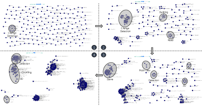
Figure 9: With the correlation matrix, we can visualize the RS datasets using network graphs. The node represents the RS dataset, and the link between nodes denotes the similarity between nodes. Datasets gradually cluster together when the connecting threshold decreases.

In Fig. 8, the correlation matrix between 401 datasets is visualized. The lighter the color, the higher the similarity. To our knowledge, this is the first work that analyzes the correlation between all existing RS datasets. The correlation matrix reflects the distances between different pairs of the RS dataset. The distance information could be valuable for the RS community. Some possible ways to leverage the correlation between RS datasets for future research are outlined below.

1. Dataset recommendation. Based on the relationships between datasets and given one dataset, we are able to recommend similar and related datasets. This will help researchers find desired datasets for their research tasks.

2. Domain adaptation. Domain adaption aims to improve the performance of a model on a target domain using the knowledge learned in the source domain. With the correlation map, researchers can easily find the proper source and target datasets for developing novel domain adaptation algorithms.

3. Dataset assembling. The distance between datasets can also be used to assemble multiple small but similar datasets into a larger one for training large-scale deep networks.

4. Multi-task model training. Similarly, using the distance between datasets, we can also combine datasets with similar spatial resolution, data modalities or research domains, but different tasks into a unified dataset for training multi-task deep models.

Furthermore, with the correlation matrix, we can visualize the RS datasets using an interactive network graph. The node represents the RS dataset, and the link between nodes denotes the similarity between them. In Fig. 9, we can see that different datasets gradually cluster together when the connecting threshold decreases.

4 Dataset Ranking and Benchmark Building

Researchers in the RS community have been publishing more and more datasets to benefit the development of new methods. However, algorithms can easily saturate their performance on these datasets [327]. Deep learning models can achieve almost perfect performance on small-scale or domain-specific datasets. However, small-scale datasets are more likely to have bias and cannot reflect the performance of methods in real-world complex scenarios [17]. Methods developed on small datasets or specific domains are difficult to generalize to other scenarios. Considering these disadvantages, it is urgent to employ new benchmarks with large-scale, general research domain, and datasets with high quality annotation for a fair and consistent evaluation of RS methods. Although the attributes of a large number of datasets are provided, it is still not intuitive to compare the quality of different datasets. Thus, for the first time, in this study, we propose to rank these datasets based on their attributes.

4.1 Dataset Ranking Metrics

Regarding the desirable properties of benchmark datasets, Long et al. [17] propose the DiRS formula, so named for its focus on the diversity, richness, and scalability of datasets. These properties are good references for designing metrics to measure and rank the RS dataset. However, it is non-trivial to quantitatively measure the diversity and richness of existing datasets. In order to approximate the DiRS metric, we consider both data diversity and annotation diversity in this study.

To measure the data diversity, we first examine the research domain of one dataset. Some datasets constructed with specific domains will have limitations on the diversity of data sources. Hence, we first filter them and only keep datasets designed for general purposes, like LULC or general scene understanding. Next, we choose to measure the dataset scale using the number, size of samples, and the volume of the dataset, i.e., attribute variables $n,s,v$. Furthermore, we take the modality diversity, that is, the number of data modalities $k$, into consideration. Since images with higher spatial resolution can provide richer visual content, we also factor in the resolution $r$ as a part of the metric.

Considering the annotation richness, we use the number of annotation classes $c$ and the quantified annotation level $m$ to measure the richness of the labels. To start with, given 401 RS datasets, we first filter out datasets designed for specific domains. After this step, 114 datasets remain as candidates. Then, we use the aforementioned attributes to quantitatively measure the diversity and richness of each dataset. Since there exist significantly high values in the $n,s,v$ of different datasets, we use log normalization to standardize them into the range 0 to 1. Next, we normalize each of the dataset attributes in $r,m,c,k$ into the range 0 to 1. Finally, we add them together to form the final score for the given dataset.

Based on the measurement defined above, we can compute the scores and rank these RS datasets. Based on the rankings, we select datasets for three different tasks. Specifically, for the RS image classification task, the top five ranked datasets are: 1). fMoW [135], 2) BigEarthNet [42], 3) Million AID [17], 4) So2Sat LCZ42 [23], and 5) RSD46-WHU [40]. For the RS object detection task, the top five datasets are 1) fMoW [135], 2) DIOR [18], 3) xView [134], 4) DOTA v2.0 [165], and 5) TGRS HRRSD [133]. Finally, for the RS semantic segmentation task, the top five ranked datasets are 1) SEASONET [25], 2) OpenSentinelMap [285], 3) SEN12MS [146], 4) GeoNRW [281], and 5) Five-Billion-Pixels [283]. A complete list of the charts is displayed on https://earthnets.github.io, where the radar charts are used to compare the attributes of some top ranked datasets.

4.2 Dataset Selection for Benchmarking

We aim to select several datasets designed with general purpose, large diversity and high richness for developing and evaluating deep learning methods. Although there are many large-scale RS datasets that meet these standards, it is unacceptable and not environment-friendly to benchmark all of them for the evaluation of RS algorithms. Thus, in this study, we choose to select two datasets for each task, including one with high-resolution and one with low resolution for larger geographical coverage.

Following this constraint, the following datasets are selected. 1) fMoW with high resolution ($\sim$1m) data and BigEarthNet with low resolution (>10m) imagery are selected for image classification. 2) DIOR with high-resolution ($\sim$1m) data and fMoW with large objects are selected for the RS object detection task. 3) GeoNRW with high-resolution ($\sim$1m) images and SEASONET with low-resolution (>10m) images are selected for RS semantic segmentation. In total, there are five datasets selected to build a unified benchmark for three different tasks.

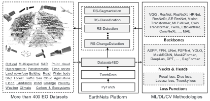
Figure 10: The architecture design of the proposed EarthNets platform. EarthNets is based on PyTorch [328] and TorchData. It contains the Dataset4EO for a standard and easy-to-use dataset loading library, and some high-level libraries for different EO tasks.

5 The EarthNets Open Platform

Large-scale, high-quality datasets are important for a faithful evaluation of RS algorithms, while other factors like training tricks, hyper-parameters, optimizers, and initialization methods are also critical for a fair and reliable comparison of different methods. Thus, an open platform is crucial for the fair evaluation, reproducibility, and efficient development of novel methods. However, there is still no unified deep learning platform for different RS tasks. Torchgeo [26] mainly focuses on the data loading part. AiTLAS[327] mainly contains codebase for the RS classification task. In contrast, we aim to build a new unified platform for the RS community that not only deals with dataset loading, but also includes libraries for different RS tasks.

Fig. 10 illustrates the overall architecture design of the proposed EarthNets platform. The platform is based on PyTorch [328] and TorchData. The library Dataset4EO is designed as a standard and easy-to-use dataset loading library. Note that Dataset4EO can be used alone or together with our high-level libraries, like RS-Classification, RS-Detection, and so on.

For the design of the EarthNets platform, we consider two main factors. The first is the decoupling between dataset loading and high-level EO tasks. As shown in this study, there are more than 400 RS datasets with different file formats, data modalities, research domains, and download links. Building a standard and scalable dataset loading library can largely accelerate research for the whole RS community. Furthermore, researchers from other machine learning community can also benefit from the standard dataset loading library. The second factor considered is pushing the RS data to a larger machine learning community. There are a number of novel deep learning models published in the CV and machine learning community, including different backbones, models, and loss functions. The EarthNets platform is designed to easily apply these models to RS datasets, and in order to fill in the gap between the RS and CV communities.

6 Experiments

In this section, we benchmark state-of-the-art deep learning models from the CV community on five selected RS datasets. We also compare them with the methods specifically designed for the RS datasets. The implementation details can be found in the supplementary materials.

TABLE V: Image Classification Results on the fMoW [135] Dataset. Top-1 accuracy, precision, recall, and F1 score are reported. The best results are in bold.

	Image Classification
Methods	Pre-trained	Top-1	P	R	F1
ViT-Small	Random	54.1	53.45	51.8	52.03
MLP-Mixer	Random	43.11	40.33	41.09	40.18
ResNet-50	ImageNet	58.25	58.73	57	57.28
EfficientNet-b4	ImageNet	58.8	58.7	57.01	57.33
ConvNext-Small	ImageNet	62.05	63.81	60.34	61.19
Swin-Tiny	ImageNet	66.42	66.33	65.29	65.5

Metrics: For multi-label image classification datasets, we report the following metrics: precision (P), recall (R), F1 score, and mean average precision (mAP). For precision, recall, and F1, we set the threshold value to 0.5 for all models. For object detection, mAP is used as the measurement for performance evaluation. Three metrics are used to evaluate the semantic segmentation task: overall (micro-averaged) Accuracy (aAcc), mean (macro-averaged) Accuracy(mAcc), and mean Intersection over Union (mIoU).

TABLE VI: Multi-label Image Classification Results on the BigEarthNet[42] Dataset. mAP, micro precision, micro recall and F1 score are reported. The best results are in bold.

	Image Classification
Methods	Pre-trained	mAP	P	R	F1
ResNet-18*[238]	Random	79.80	-	-	-
ResNet-18*[238]	ImageNet	85.90	-	-	-
ResNet-18*[238]	MoCo-v2	85.23	-	-	-
ResNet-50*[238]	ImageNet	86.74	-	-	-
ResNet-50	ImageNet	85.74	76.87	75.89	76.38
EfficientNet-b4	ImageNet	84.48	73.84	77.19	75.48
ConvNext-Small	ImageNet	85.59	73.64	79.91	76.65
Swin-Tiny	ImageNet	87.19	78.01	80.22	79.1
MLP Mixer	ImageNet	82.76	73	74.36	73.67

6.1 Benchmarking Results and Comparisons

In this section, we benchmark the five selected datasets using the proposed EarthNets platform. In order to avoid excessive computation costs, we choose to evaluate some representative state-of-the-art (SOTA) methods from the CV community on the large-scale RS datasets.

TABLE VII: Object Detection Results on the DIOR[18] Dataset. The mAP performance is reported. The best results are in bold.

Method	Object Detection
	Backbone	Optimizer	Epochs	mAP
RetinaNet* [18]	ResNet-50	-	-	65.7
RetinaNet* [18]	ResNet-101	-	-	66.1
PANet* [18]	ResNet-50	-	-	63.8
PANet* [18]	ResNet-101	-	-	66.1
Mask-RCNN* [18]	ResNet-50	-	-	63.5
Mask-RCNN* [18]	ResNet-101	-	-	65.2
YoloV3* [18]	DarkNet53	-	-	57.1
YoloV3	DarkNet53	SGD	120	64.0
YoloV3	Swin-Tiny	AdamW	120	64.6
YoloV3	ConvNext-Small	AdamW	120	67.6
Mask-RCNN	ResNet-50	SGD	120	68.5
Mask-RCNN	Swin-Tiny	AdamW	120	70.5
Mask-RCNN	ConvNext-Small	AdamW	120	72.4

TABLE VIII: Semantic Segmentation Results on the SEASONET[25] Dataset. We report the aAcc, mAcc and mIoU metrics. The best results are in bold.

Method	Semantic Segmentation
	Backbone	Optimizer	Iter.	aAcc	mAcc	mIoU
DeeplabV3* [25]	DenseNet121	–	–	–	–	47.53
DeeplabV3,PT* [25]	DenseNet121	–	–	–	–	48.69
DeeplabV3	ResNet-50	SGD	80k	82.87	58.49	47.5
DeeplabV3	ResNet-50	SGD	160k	83.52	62.65	50.79
DeeplabV3	ConvNext-Small	AdamW	120k	81.36	56.31	46.39
DeeplabV3	Swin-Tiny	AdamW	120k	82.75	61.5	50.81
Upernet	ResNet-50	SGD	120k	83.2	60.36	49.59
SegFormer	MiT	AdamW	120k	83.75	64.25	53.87

TABLE IX: Semantic Segmentation Results on the GeoNRW[281] Dataset. We report the aAcc, mAcc and mIoU metrics. The best results are in bold.

	Semantic Segmentation
Method	Backbone	Optimizer	#Epochs	aAcc	mAcc	mIoU
MultiTask* [329]	Transfomer	AdamW	100k	76.75	71.89	57.3
Lu et al.* [329]	Transfomer	AdamW	100k	76.53	70.12	56.2
FCN	UNet	SGD	40k	78.8	66.86	55.6
PSPNet	ResNet-50	SGD	40k	81.56	74.92	62.73
Deeplabv3+	ResNet-50	SGD	40k	81.91	75.26	63.01
Deeplabv3+	ConvNext-Tiny	AdamW	40k	80.89	73.61	61.63
Deeplabv3+	Swin-Tiny	SGD	40k	78.09	70.01	56.78
Deeplabv3+	Swin-Tiny	AdamW	40k	81.11	74.28	62.18
Upernet	ResNet-50	SGD	40k	81.87	75.7	63.1
Upernet	ConvNext-Tiny	AdamW	40k	82.08	74.9	63.48
Upernet	Vit-Small	AdamW	40k	78.65	71.13	59.43
Upernet	Swin-Tiny	AdamW	40k	82.31	75.68	64.48
SegFormer	MiT	AdamW	40k	82.55	75.63	64.38

Comparisons on the fMoW Dataset. fMoW [135] is a large-scale dataset built for recognizing the functional purpose of buildings and land use. It contains 1 million images from over 200 countries, annotated with 63 different classes. In this study, we use the fMoW-rgb version of the dataset for model evaluation. Table V reports the benchmarking results. In general, we can see that using the ImageNet pre-trained weights can greatly improve the performance. When we compare the CNN-based methods with the Transformer-based method, we find that Swin-Tiny [330] clearly outperforms other CNN-based methods in all the four metrics. Among the CNN-based methods, ConvNext [331] is the best performing one.

Comparisons on the BigEarthNet Dataset. BigEarthNet is a large-scale multi-label Sentinel-2 benchmark dataset annotated with the CORINE Land Cover classes. There are two versions of the labels, one with 43 categories and another with 19 categories. In this study, we adopt the new class nomenclature (19 categories) introduced in [332]. Regarding the methods, we evaluate four CNN-based architectures (ResNet-18, ResNet-50, EfficientNet-b4, ConvNext). For Transformer-based method, we evaluate the Swin-Tiny, which is usually overlooked in existing benchmarking results. Furthermore, an MLP-based method, the MLP-Mixer [333] is also compared. Additionally, we also compare the results reported by existing work [238] on the BigEarthNet dataset.

Table VI reports the benchmarking results. In general, the results indicate that Swin-Tiny performs best on this multi-label classification dataset. However, there is no significant advantage compared with other CNN-based methods. Another conclusion we can make is that ResNet-50 is a strong baseline method. From the results, it can be seen that ResNet-50, pre-trained on ImageNet or using self-supervised MoCo-V2 [334], can perform better than MLP-Mixer, EfficientNet-b4 on this dataset. The performance of ConvNext is competitive to ResNet-50, but lower than the transformer-based method Swin-Tiny. Note that ^∗ indicates that the results of the method are reported in existing work. Generally speaking, the results benchmarked using the EarthNets platform are higher than or comparable to existing reported results.

Comparisons on the DIOR Dataset. Table VII presents the benchmarking results on the DIOR dataset built for the object detection task. We choose two representative and widely-used object detection methods designed by the CV community. To be specific, YoloV3[113] and Mask-RCNN[335] are evaluated on the DIOR dataset. YoloV3 is designed for light-weight and real-time object detection. Mask-RCNN is an extension of Faster-RCNN [111] with ROI align and a third segmentation branch. The experimental results reveal that Mask-RCNN performs better than YoloV3 on this dataset. With regard to different backbones, the results clearly show that Swin-Tiny and ConvNext can outperform other compared methods. The Mask-RCNN method with ConvNext backbone achieves an mAP of 72.4%, which is 6.3 percentage points higher than the best results reported in [18]. Notably, we observe that our benchmarked results can greatly outperform the same method reported in existing work. This comparison reveals that the choice of the optimizer, hyper-parameters, or other training tricks can greatly affect the final results, even when the same method is used.

Comparisons on the SEASONET Dataset. SEASONET is a large-scale multi-label LULC scene understanding dataset. It includes 1,759,830 images from Sentinel-2 tiles, and can be used for scene classification, segmentation, and retrieval tasks. In this study, we evaluate segmentation performance on this dataset. On this dataset, we evaluate the widely-used semantic segmentation method DeeplabV3 [336] with three different backbones: ResNet-50, ConvNext, and Swin-Tiny. Upernet and SegFormer [337] with mixed-Transformer encoders (MiT) are also compared. Table VIII reports the benchmarking results. It can be seen that ResNet-50 and Swin-Tiny obtain comparable results and clearly surpass other backbones. SegFormer with MiT encoder clearly outperforms other models. We also find that the results obtained using EarthNets significantly outperform performance reported in existing work [25].

Comparisons on the GeoNRW Dataset. The benchmarking results on the GeoNRW dataset are displayed in Table IX. Five segmentation methods, FCN [338], DeeplabV3+ [339], PSPNet [340], Upernet [341] and SegFormer [337] with mixed-Transformer encoders (MiT), are evaluated on this dataset. We observe that Transformer-based models like SegFormer and Swin Transformer perform better than other methods. However, the performance of ViT-Small is worse than ResNet-50. In comparison to the reported results in existing work, we can find that using the EarthNets platform can obtain clearly better performance.

7 Conclusion

In this study, we present a comprehensive review and build a taxonomy for more than 400 publicly published datasets in the remote sensing community. Based on the attribute information of these datasets, we systemically analyze them with respect to five aspects: volumes, bibliometric analysis, resolution distributions, research domains, and the correlation between datasets. Next, a new benchmark including five selected large-scale datasets is built for model evaluation. A deep learning platform termed EarthNets is released with the intention to support a consistent evaluation of deep learning methods on remote sensing data. We further use the EarthNets platform to benchmark state-of-the-art methods on the new benchmark. The performance comparisons are insightful for future research.

References

- [1] C. Toth and G. Jóźków, “Remote sensing platforms and sensors: A survey,” ISPRS J. Photogramm. Remote Sens., vol. 115, pp. 22–36, 2016.
- [2] X. X. Zhu, D. Tuia, L. Mou, G.-S. Xia, L. Zhang, F. Xu, and F. Fraundorfer, “Deep learning in remote sensing: A comprehensive review and list of resources,” IEEE GRSM, vol. 5, no. 4, pp. 8–36, 2017.
- [3] A. Shaker, W. Y. Yan, and P. E. LaRocque, “Automatic land-water classification using multispectral airborne lidar data for near-shore and river environments,” ISPRS J. Photogramm. Remote Sens., vol. 152, pp. 94–108, 2019.
- [4] M. E. Bauer, “Remote sensing of environment: history, philosophy, approach and contributions, 1969–2019,” Remote Sens. Environ., vol. 237, p. 111522, 2020.
- [5] M. Wójtowicz, A. Wójtowicz, J. Piekarczyk et al., “Application of remote sensing methods in agriculture,” Communications in Biometry and Crop Science, vol. 11, no. 1, pp. 31–50, 2016.
- [6] L. Karthikeyan, I. Chawla, and A. K. Mishra, “A review of remote sensing applications in agriculture for food security: Crop growth and yield, irrigation, and crop losses,” Journal of Hydrology, vol. 586, p. 124905, 2020.
- [7] K. E. Joyce, K. C. Wright, S. V. Samsonov, and V. G. Ambrosia, “Remote sensing and the disaster management cycle,” Advances in geoscience and remote sensing, vol. 48, p. 7, 2009.
- [8] C. Van Westen, “Remote sensing for natural disaster management,” ISPRS Archives, vol. 33, no. B7/4; PART 7, pp. 1609–1617, 2000.
- [9] A. Krizhevsky, I. Sutskever, and G. E. Hinton, “Imagenet classification with deep convolutional neural networks,” Communications of the ACM, vol. 60, no. 6, pp. 84–90, 2017.
- [10] L. Zhang, L. Zhang, and B. Du, “Deep learning for remote sensing data: A technical tutorial on the state of the art,” IEEE GRSM, vol. 4, no. 2, pp. 22–40, 2016.
- [11] Z. Xiong, Y. Yuan, and Q. Wang, “AI-NET: Attention inception neural networks for hyperspectral image classification,” in IGARSS. IEEE, 2018, pp. 2647–2650.
- [12] G. Marchisio, P. Helber, B. Bischke, T. Davis, C. Senaras, D. Zanaga, R. Van De Kerchove, and A. Wania, “Rapidai4eo: A corpus for higher spatial and temporal reasoning,” in 2021 IEEE International Geoscience and Remote Sensing Symposium IGARSS. IEEE, 2021, pp. 1161–1164.
- [13] A. Hecheltjen, F. Thonfeld, and G. Menz, “Recent advances in remote sensing change detection–a review,” Land use and land cover mapping in Europe, pp. 145–178, 2014.
- [14] M. Rahnemoonfar, T. Chowdhury, A. Sarkar, D. Varshney, M. Yari, and R. R. Murphy, “Floodnet: A high resolution aerial imagery dataset for post flood scene understanding,” IEEE Access, vol. 9, pp. 89 644–89 654, 2021.
- [15] K. Bakula, J. Mills, and F. Remondino, “A review of benchmarking in photogrammetry and remote sensing,” ISPRS Archives, 2019.
- [16] M. Schmitt, S. A. Ahmadi, and R. Hänsch, “There is no data like more data-current status of machine learning datasets in remote sensing,” in IGARSS. IEEE, 2021, pp. 1206–1209.
- [17] Y. Long, G.-S. Xia, S. Li, W. Yang, M. Y. Yang, X. X. Zhu, L. Zhang, and D. Li, “On creating benchmark dataset for aerial image interpretation: Reviews, guidances, and million-aid,” IEEE J. Sel. Top. Appl. Earth Obs. Remote Sens., vol. 14, pp. 4205–4230, 2021.
- [18] K. Li, G. Wan, G. Cheng, L. Meng, and J. Han, “Object detection in optical remote sensing images: A survey and a new benchmark,” ISPRS J. Photogramm. Remote Sens., vol. 159, pp. 296–307, 2020.
- [19] A. Abdollahi, B. Pradhan, N. Shukla, S. Chakraborty, and A. Alamri, “Deep learning approaches applied to remote sensing datasets for road extraction: A state-of-the-art review,” Remote Sensing, vol. 12, no. 9, p. 1444, 2020.
- [20] I. Tomljenovic, B. Höfle, D. Tiede, and T. Blaschke, “Building extraction from airborne laser scanning data: An analysis of the state of the art,” Remote Sensing, vol. 7, no. 4, pp. 3826–3862, 2015.
- [21] M. Schmitt, P. Ghamisi, N. Yokoya, and R. Hänsch, “Eod: The ieee grss earth observation database,” in IGARSS. IEEE, 2022, pp. 5365–5368.
- [22] J. Deng, W. Dong, R. Socher, L.-J. Li, K. Li, and L. Fei-Fei, “Imagenet: A large-scale hierarchical image database,” in CVPR. Ieee, 2009, pp. 248–255.
- [23] X. X. Zhu, J. Hu, C. Qiu, Y. Shi, J. Kang, L. Mou, H. Bagheri, M. Häberle, Y. Hua, R. Huang et al., “So2sat lcz42: A benchmark dataset for global local climate zones classification,” arXiv preprint arXiv:1912.12171, 2019.
- [24] G. Christie, N. Fendley, J. Wilson, and R. Mukherjee, “Functional map of the world,” in CVPR, 2018, pp. 6172–6180.
- [25] D. Koßmann, V. Brack, and T. Wilhelm, “Seasonet: A seasonal scene classification, segmentation and retrieval dataset for satellite imagery over germany,” in IGARSS. IEEE, 2022, pp. 243–246.
- [26] A. J. Stewart, C. Robinson, I. A. Corley, A. Ortiz, J. M. L. Ferres, and A. Banerjee, “Torchgeo: deep learning with geospatial data,” arXiv preprint arXiv:2111.08872, 2021.
- [27] Y. Yang and S. Newsam, “Bag-of-visual-words and spatial extensions for land-use classification,” in ACM SIGSPATIAL, 2010, pp. 270–279.
- [28] G.-S. Xia, J. Hu, F. Hu, B. Shi, X. Bai, Y. Zhong, L. Zhang, and X. Lu, “Aid: A benchmark data set for performance evaluation of aerial scene classification,” IEEE TGRS, vol. 55, no. 7, pp. 3965–3981, 2017.
- [29] G.-S. Xia, X. Bai, J. Ding, Z. Zhu, S. Belongie, J. Luo, M. Datcu, M. Pelillo, and L. Zhang, “Dota: A large-scale dataset for object detection in aerial images,” in CVPR, June 2018.
- [30] M. V. M Grana and B. Ayerdi. (2022) Hyperspectral datasets. [Online]. Available: http://www.ehu.eus/ccwintco/index.php/Hyperspectral_Remote_Sensing_Scenes
- [31] X. Sun, Y. Lv, Z. Wang, and K. Fu, “Scan: Scattering characteristics analysis network for few-shot aircraft classification in high-resolution sar images,” IEEE TGRS, vol. 60, pp. 1–17, 2022.
- [32] (2015) District of columbia – classified point cloud lidar. [Online]. Available: https://github.com/awslabs/open-data-docs/tree/main/docs/dc-lidar-2018
- [33] ISPRS-Contest. (2022) Isprs 2d semantic labeling contest,” accessed on oct. 9, 2022. [Online]. Available: https://www.isprs.org/education/benchmarks/UrbanSemLab/2d-sem-label-potsdam.aspx
- [34] ——. (2022) Isprs 2d semantic labeling contest,” accessed on oct. 9, 2022. [Online]. Available: https://www.isprs.org/education/benchmarks/UrbanSemLab/2d-sem-label-vaihingen.aspx
- [35] O. A. Penatti, K. Nogueira, and J. A. Dos Santos, “Do deep features generalize from everyday objects to remote sensing and aerial scenes domains?” in CVPRW, 2015, pp. 44–51.
- [36] L. Kondmann, A. Toker, M. Rußwurm, A. Camero Unzueta, D. Peressuti, G. Milcinski, N. Longépé, P.-P. Mathieu, T. Davis, G. Marchisio et al., “DENETHOR: The DynamicEarthNET dataset for Harmonized, inter-Operable, analysis-Ready, daily crop monitoring from space,” in NeurIPS Datasets and Benchmarks Track, 2021.
- [37] D. Sykas, I. Papoutsis, and D. Zografakis, “Sen4agrinet: A harmonized multi-country, multi-temporal benchmark dataset for agricultural earth observation machine learning applications,” in IGARSS. IEEE, 2021, pp. 5830–5833.
- [38] E. L. Amanda A. Boatswain Jacques, Abdoulaye Baniré Diallo, “Towards the creation of a canadian land-use dataset for agricultural land classification,” in Canadian Symposium on Remote Sensing, 2021.
- [39] X. Qi, P. Zhu, Y. Wang, L. Zhang, J. Peng, M. Wu, J. Chen, X. Zhao, N. Zang, and P. T. Mathiopoulos, “Mlrsnet: A multi-label high spatial resolution remote sensing dataset for semantic scene understanding,” ISPRS J. Photogramm. Remote Sens., vol. 169, pp. 337–350, 2020.
- [40] Z. Xiao, Y. Long, D. Li, C. Wei, G. Tang, and J. Liu, “High-resolution remote sensing image retrieval based on cnns from a dimensional perspective,” Remote Sensing, vol. 9, no. 7, p. 725, 2017.
- [41] G. Cheng, J. Han, and X. Lu, “Remote sensing image scene classification: Benchmark and state of the art,” Proceedings of the IEEE, vol. 105, no. 10, pp. 1865–1883, 2017.
- [42] G. Sumbul, M. Charfuelan, B. Demir, and V. Markl, “Bigearthnet: A large-scale benchmark archive for remote sensing image understanding,” in IGARSS. IEEE, 2019, pp. 5901–5904.
- [43] G. Machado, E. Ferreira, K. Nogueira, H. Oliveira, M. Brito, P. H. T. Gama, and J. A. dos Santos, “Airound and cv-brct: Novel multiview datasets for scene classification,” IEEE J. Sel. Top. Appl. Earth Obs. Remote Sens., vol. 14, pp. 488–503, 2020.
- [44] P. Helber, B. Bischke, A. Dengel, and D. Borth, “Eurosat: A novel dataset and deep learning benchmark for land use and land cover classification,” IEEE J. Sel. Top. Appl. Earth Obs. Remote Sens., vol. 12, no. 7, pp. 2217–2226, 2019.
- [45] R. Bahmanyar, D. Espinoza-Molina, and M. Datcu, “Multisensor earth observation image classification based on a multimodal latent dirichlet allocation model,” IEEE Geosci. Remote Sens. Lett., vol. 15, no. 3, pp. 459–463, 2018.
- [46] Y. Zhong, Q. Zhu, and L. Zhang, “Scene classification based on the multifeature fusion probabilistic topic model for high spatial resolution remote sensing imagery,” IEEE TGRS, vol. 53, no. 11, pp. 6207–6222, 2015.
- [47] H. Li, X. Dou, C. Tao, Z. Wu, J. Chen, J. Peng, M. Deng, and L. Zhao, “Rsi-cb: A large-scale remote sensing image classification benchmark using crowdsourced data,” Sensors, vol. 20, no. 6, p. 1594, 2020.
- [48] (2018) Ships in satellite imagery. [Online]. Available: https://www.kaggle.com/datasets/rhammell/ships-in-satellite-imagery
- [49] A. P. Antonio-Javier Gallego and P. Gil, “Automatic ship classification from optical aerial images with convolutional neural networks,” Remote Sensing, vol. 10, no. 4, 2018.
- [50] Y. Di, Z. Jiang, H. Zhang, and G. Meng, “A public dataset for ship classification in remote sensing images,” in SPIE, vol. 11155, 2019, pp. 515–521.
- [51] I. G. Rizaev and A. Achim, “Synthwakesar: A synthetic sar dataset for deep learning classification of ships at sea,” Remote Sensing, vol. 14, no. 16, p. 3999, 2022.
- [52] Q. D. Cao and Y. Choe, “Building damage annotation on post-hurricane satellite imagery based on convolutional neural networks,” Natural Hazards, vol. 103, no. 3, pp. 3357–3376, 2020.
- [53] C. Rambour, N. Audebert, E. Koeniguer, B. Le Saux, M. Crucianu, and M. Datcu, “Flood detection in time series of optical and sar images,” ISPRS Archives, vol. 43, pp. 1343–1346, 2020.
- [54] D. Bonafilia, B. Tellman, T. Anderson, and E. Issenberg, “Sen1floods11: A georeferenced dataset to train and test deep learning flood algorithms for sentinel-1,” in CVPRW, 2020, pp. 210–211.
- [55] R. Ba, C. Chen, J. Yuan, W. Song, and S. Lo, “Smokenet: Satellite smoke scene detection using convolutional neural network with spatial and channel-wise attention,” Remote Sensing, vol. 11, no. 14, p. 1702, 2019.
- [56] (2017) Noaa fisheries steller sea lion population count. [Online]. Available: https://www.kaggle.com/c/noaa-fisheries-steller-sea-lion-population-count/data
- [57] N. Imamoglu, M. Kimura, H. Miyamoto, A. Fujita, and R. Nakamura, “Solar power plant detection on multi-spectral satellite imagery using weakly-supervised cnn with feedback features and m-pcnn fusion,” arXiv preprint arXiv:1704.06410, 2017.
- [58] (2018) Airbus wind turbines patches. [Online]. Available: https://www.kaggle.com/datasets/airbusgeo/airbus-wind-turbines-patches
- [59] M. F. Baumgardner, L. L. Biehl, and D. A. Landgrebe, “220 band aviris hyperspectral image data set: June 12, 1992 indian pine test site 3,” Purdue University Research Repository, vol. 10, no. 7, p. 991, 2015.
- [60] R. M Rustowicz, R. Cheong, L. Wang, S. Ermon, M. Burke, and D. Lobell, “Semantic segmentation of crop type in africa: A novel dataset and analysis of deep learning methods,” in CVPRW, 2019, pp. 75–82.
- [61] H. Kerner, C. Nakalembe, and I. Becker-Reshef, “Field-level crop type classification with k nearest neighbors: a baseline for a new kenya smallholder dataset,” arXiv preprint arXiv:2004.03023, 2020.
- [62] M. Rußwurm, C. Pelletier, M. Zollner, S. Lefèvre, and M. Körner, “Breizhcrops: A time series dataset for crop type mapping,” ISPRS (2020), 2020.
- [63] S. Virnodkar, V. Pachghare, V. Patil, and S. K. Jha, “Canesat,” 2020. [Online]. Available: https://dx.doi.org/10.21227/vzbn-qj64
- [64] G. Tseng, I. Zvonkov, C. L. Nakalembe, and H. Kerner, “Cropharvest: A global dataset for crop-type classification,” in NeurIPS Datasets and Benchmarks Track, 2021.
- [65] R. E. F. Western Cape Department of Agricultures. (2021) Crop type classification dataset for western cape, south africa. [Online]. Available: https://doi.org/10.34911/rdnt.j0co8q
- [66] G. Choumos, A. Koukos, V. Sitokonstantinou, and C. Kontoes, “Towards space-to-ground data availability for agriculture monitoring,” in IVMSP, 2022, pp. 1–5.
- [67] M. J. Hughes and D. J. Hayes, “Automated detection of cloud and cloud shadow in single-date landsat imagery using neural networks and spatial post-processing,” Remote Sensing, vol. 6, no. 6, pp. 4907–4926, 2014.
- [68] M. P. I. for Meteorology. (2019) Understanding clouds from satellite images. [Online]. Available: https://www.kaggle.com/c/understanding_cloud_organization/data
- [69] A. H. Nielsen, A. Iosifidis, and H. Karstoft, “Cloudcast: A satellite-based dataset and baseline for forecasting clouds,” IEEE J. Sel. Top. Appl. Earth Obs. Remote Sens., vol. 14, pp. 3485–3494, 2021.
- [70] (2020) Sentinel-2 cloud mask catalogue. [Online]. Available: https://zenodo.org/record/4172871#.Y0LEOHbP1D-
- [71] L. Mou, Y. Hua, P. Jin, and X. X. Zhu, “ERA: A dataset and deep learning benchmark for event recognition in aerial videos,” IEEE GRSM, in press.
- [72] G. I. Drakonakis, G. Tsagkatakis, K. Fotiadou, and P. Tsakalides, “Ombrianet—supervised flood mapping via convolutional neural networks using multitemporal sentinel-1 and sentinel-2 data fusion,” IEEE J. Sel. Top. Appl. Earth Obs. Remote Sens., vol. 15, pp. 2341–2356, 2022.
- [73] S. Chandak, V. Chitters, and S. Honnungar, “Understanding the amazon rainforest from space using cnns,” 2017.
- [74] D. Noever and S. E. M. Noever, “Overhead mnist: A benchmark satellite dataset,” arXiv preprint arXiv:2102.04266, 2021.
- [75] G.-S. Xia, W. Yang, J. Delon, Y. Gousseau, H. Sun, and H. MaÎtre, “Structural high-resolution satellite image indexing,” Vienna, Austria, 2010.
- [76] Q. Zou, L. Ni, T. Zhang, and Q. Wang, “Deep learning based feature selection for remote sensing scene classification,” IEEE Geosci. Remote Sens. Lett., vol. 12, no. 11, pp. 2321–2325, 2015.
- [77] L. Zhao, P. Tang, and L. Huo, “Feature significance-based multibag-of-visual-words model for remote sensing image scene classification,” Journal of Applied Remote Sensing, vol. 10, no. 3, p. 035004, 2016.
- [78] W. Zhou, S. Newsam, C. Li, and Z. Shao, “Patternnet: A benchmark dataset for performance evaluation of remote sensing image retrieval,” ISPRS J. Photogramm. Remote Sens., vol. 145, pp. 197–209, 2018.
- [79] Q. Wang, S. Liu, J. Chanussot, and X. Li, “Scene classification with recurrent attention of vhr remote sensing images,” IEEE TGRS, vol. 57, no. 2, pp. 1155–1167, 2018.
- [80] H. Li, H. Jiang, X. Gu, J. Peng, W. Li, L. Hong, and C. Tao, “Clrs: Continual learning benchmark for remote sensing image scene classification,” Sensors, vol. 20, no. 4, p. 1226, 2020.
- [81] Z. Zhou, S. Li, W. Wu, W. Guo, X. Li, G. Xia, and Z. Zhao, “Nasc-tg2: Natural scene classification with tiangong-2 remotely sensed imagery,” IEEE J. Sel. Top. Appl. Earth Obs. Remote Sens., vol. 14, pp. 3228–3242, 2021.
- [82] M. Reda. (2021) Satellite image classification. [Online]. Available: https://www.kaggle.com/datasets/mahmoudreda55/satellite-image-classification
- [83] Y. Hua, L. Mou, P. Jin, and X. X. Zhu, “Multiscene: A large-scale dataset and benchmark for multiscene recognition in single aerial images,” IEEE TGRS, vol. 60, pp. 1–13, 2021.
- [84] N. I. Bountos, I. Papoutsis, D. Michail, A. Karavias, P. Elias, and I. Parcharidis, “Hephaestus: A large scale multitask dataset towards insar understanding,” in CVPR, 2022, pp. 1453–1462.
- [85] K. Uehara, H. Sakanashi, H. Nosato, M. Murakawa, H. Miyamoto, and R. Nakamura, “Object detection of satellite images using multi-channel higher-order local autocorrelation,” in IEEE SMC. IEEE, 2017, pp. 1339–1344.
- [86] Statoil. (2017) Statoil/c-core iceberg classifier challenge. [Online]. Available: https://www.kaggle.com/competitions/statoil-iceberg-classifier-challenge
- [87] S. Basu, S. Ganguly, S. Mukhopadhyay, R. DiBiano, M. Karki, and R. Nemani, “Deepsat: a learning framework for satellite imagery,” in ACM SIGSPATIAL, 2015, pp. 1–10.
- [88] (2017) Tiselac: Time series land cover classification challeng. [Online]. Available: https://sites.google.com/site/dinoienco/tiselc
- [89] X.-Y. Tong, G.-S. Xia, Q. Lu, H. Shen, S. Li, S. You, and L. Zhang, “Land-cover classification with high-resolution remote sensing images using transferable deep models,” Remote Sens. Environ., vol. 237, p. 111322, 2020.
- [90] (2019) Eopatches for slovenia 2019. [Online]. Available: http://eo-learn.sentinel-hub.com/
- [91] (2016) Tianggong1 high-resolution satellite scene classification. [Online]. Available: http://www.msadc.cn/main/setsubDetail?id=1369487569196158978
- [92] (2017) Austin zoning satellite images. [Online]. Available: https://www.kaggle.com/datasets/franchenstein/austin-zoning-satellite-images
- [93] R. Ratajczak, C. F. Crispim-Junior, É. Faure, B. Fervers, and L. Tougne, “Automatic Land Cover Reconstruction From Historical Aerial Images: An Evaluation of Features Extraction and Classification Algorithms,” IEEE Trans. Image Process., Jan. 2019.
- [94] (2020) Sense earth satellite scene classification. [Online]. Available: https://aistudio.baidu.com/aistudio/datasetdetail/52728
- [95] S. Ji, D. Yu, C. Shen, W. Li, and Q. Xu, “Landslide detection from an open satellite imagery and digital elevation model dataset using attention boosted convolutional neural networks,” Landslides, vol. 17, no. 6, pp. 1337–1352, 2020.
- [96] U. S. Ranjan and A. Narayana, “Classification of objects in sar images using scaling features.” in ICVGIP, 2002.
- [97] (2018) Forest cover type (kernels only). [Online]. Available: https://www.kaggle.com/c/forest-cover-type-kernels-only/data
- [98] (2019) Aerial cactus identification. [Online]. Available: https://www.kaggle.com/c/aerial-cactus-identification
- [99] (2019) Wids datathon 2019. [Online]. Available: https://www.kaggle.com/c/widsdatathon2019
- [100] S. Beery, G. Wu, T. Edwards, F. Pavetic, B. Majewski, S. Mukherjee, S. Chan, J. Morgan, V. Rathod, and J. Huang, “The auto arborist dataset: A large-scale benchmark for multiview urban forest monitoring under domain shift,” in CVPR, 2022, pp. 21 294–21 307.
- [101] S. Ahlswede, C. Schulz, C. Gava, P. Helber, B. Bischke, M. Förster, F. Arias, J. Hees, B. Demir, and B. Kleinschmit, “Treesatai benchmark archive: A multi-sensor, multi-label dataset for tree species classification in remote sensing,” Earth System Science Data Discussions, pp. 1–22, 2022.
- [102] S. F. Agency. (2021) Forest damages – larch casebearer 1.0. national forest data lab. dataset. [Online]. Available: https://lila.science/datasets/forest-damages-larch-casebearer
- [103] E. Cole, B. Deneu, T. Lorieul, M. Servajean, C. Botella, D. Morris, N. Jojic, P. Bonnet, and A. Joly, “The geolifeclef 2020 dataset,” arXiv preprint arXiv:2004.04192, 2020.
- [104] E. Ferreira, M. Brito, R. Balaniuk, M. S. Alvim, and J. A. dos Santos, “Brazildam: A benchmark dataset for tailings dam detection,” in LAGIRS. IEEE, 2020, pp. 339–344.
- [105] B. Chen, Q. Feng, B. Niu, F. Yan, B. Gao, J. Yang, J. Gong, and J. Liu, “Multi-modal fusion of satellite and street-view images for urban village classification based on a dual-branch deep neural network,” Int. J. Appl. Earth Obs. Geoinf., vol. 109, p. 102794, 2022.
- [106] (2022) Kennedy space center. [Online]. Available: https://www.csr.utexas.edu/projects/rs/hrs/classify.html
- [107] K. Nogueira, J. A. Dos Santos, T. Fornazari, T. S. F. Silva, L. P. Morellato, and R. d. S. Torres, “Towards vegetation species discrimination by using data-driven descriptors,” in PRRS. Ieee, 2016, pp. 1–6.
- [108] B. Uzkent, A. Rangnekar, and M. J. Hoffman, “Tracking in aerial hyperspectral videos using deep kernelized correlation filters,” arXiv preprint arXiv:1711.07235, 2017.
- [109] (2019) Find a car park. [Online]. Available: https://www.kaggle.com/datasets/daggysheep/find-a-car-park
- [110] E. Dahan, T. Diskin, A. Amram, A. Moryossef, and O. Koren, “Cofga: A dataset for fine grained classification of objects from aerial imagery,” arXiv preprint arXiv:2105.12786, 2021.
- [111] S. Ren, K. He, R. Girshick, and J. Sun, “Faster r-cnn: Towards real-time object detection with region proposal networks,” NeurIPS, vol. 28, 2015.
- [112] W. Liu, D. Anguelov, D. Erhan, C. Szegedy, S. Reed, C.-Y. Fu, and A. C. Berg, “SSD: Single shot multibox detector,” in ECCV. Springer, 2016, pp. 21–37.
- [113] J. Redmon, S. Divvala, R. Girshick, and A. Farhadi, “You only look once: Unified, real-time object detection,” in CVPR, 2016, pp. 779–788.
- [114] N. Carion, F. Massa, G. Synnaeve, N. Usunier, A. Kirillov, and S. Zagoruyko, “End-to-end object detection with transformers,” in ECCV. Springer, 2020, pp. 213–229.
- [115] RHAMMELL. (2017) Planes in satellite imagery. [Online]. Available: https://www.kaggle.com/datasets/rhammell/planesnet
- [116] B. A. Jeff Faudi. (2021) Airbus aircraft detection. [Online]. Available: https://www.kaggle.com/datasets/airbusgeo/airbus-aircrafts-sample-dataset
- [117] S. Rawat. (2021) Casia-aircraft. [Online]. Available: https://www.rsaicp.com/portal/dataDetail?id=16
- [118] I. Demir, K. Koperski, D. Lindenbaum, G. Pang, J. Huang, S. Basu, F. Hughes, D. Tuia, and R. Raskar, “Deepglobe 2018: A challenge to parse the earth through satellite images,” in CVPRW, June 2018.
- [119] Microsoft. (2019) Us building footprints. [Online]. Available: https://github.com/microsoft/USBuildingFootprints
- [120] (2018) Segmenting buildings in satellite images. [Online]. Available: https://www.kaggle.com/code/kmader/segmenting-buildings-in-satellite-images/data
- [121] N. Weir, D. Lindenbaum, A. Bastidas, A. V. Etten, S. McPherson, J. Shermeyer, V. Kumar, and H. Tang, “Spacenet mvoi: A multi-view overhead imagery dataset,” in ICCV, 2019, pp. 992–1001.
- [122] L. Huang, B. Liu, B. Li, W. Guo, W. Yu, Z. Zhang, and W. Yu, “Opensarship: A dataset dedicated to sentinel-1 ship interpretation,” IEEE J. Sel. Top. Appl. Earth Obs. Remote Sens., vol. 11, no. 1, pp. 195–208, 2017.
- [123] J. Li, C. Qu, and J. Shao, “Ship detection in sar images based on an improved faster r-cnn,” in BIGSARDATA. IEEE, 2017, pp. 1–6.
- [124] Airbus. (2018) Airbus ship detection challenge. [Online]. Available: https://www.kaggle.com/c/airbus-ship-detection
- [125] p. m. adrian and A. Umam. (2018) Ships in google earth. [Online]. Available: https://www.kaggle.com/datasets/tomluther/ships-in-google-earth
- [126] G. Heitz and D. Koller, “Learning spatial context: Using stuff to find things,” in ECCV. Springer, 2008, pp. 30–43.
- [127] S. Razakarivony and F. Jurie, “Vehicle detection in aerial imagery: A small target detection benchmark,” Journal of Visual Communication and Image Representation, vol. 34, pp. 187–203, 2016.
- [128] T. N. Mundhenk, G. Konjevod, W. A. Sakla, and K. Boakye, “A large contextual dataset for classification, detection and counting of cars with deep learning,” in ECCV. Springer, 2016, pp. 785–800.
- [129] DLR. (2016) Dlr multi-class vehicle detection and orientation in aerial imagery. [Online]. Available: https://www.dlr.de/eoc/en/desktopdefault.aspx/tabid-12760/22294_read-52777
- [130] M. Y. Yang, W. Liao, X. Li, and B. Rosenhahn, “Deep learning for vehicle detection in aerial images,” in ICIP, 2018.
- [131] G. Cheng and J. Han, “A survey on object detection in optical remote sensing images,” ISPRS J. Photogramm. Remote Sens., vol. 117, pp. 11–28, 2016.
- [132] Y. Long, Y. Gong, Z. Xiao, and Q. Liu, “Accurate object localization in remote sensing images based on convolutional neural networks,” IEEE TGRS, vol. 55, no. 5, pp. 2486–2498, 2017.
- [133] Y. Zhang, Y. Yuan, Y. Feng, and X. Lu, “Hierarchical and robust convolutional neural network for very high-resolution remote sensing object detection,” IEEE TGRS, vol. 57, no. 8, pp. 5535–5548, 2019.
- [134] xView. (2019) xview 2018 object detection challenge. [Online]. Available: https://challenge.xviewdataset.org/welcome
- [135] G. Christie, N. Fendley, J. Wilson, and R. Mukherjee, “Functional map of the world,” in CVPR, 2018.
- [136] W. Han, J. Li, S. Wang, Y. Wang, J. Yan, R. Fan, X. Zhang, and L. Wang, “A context-scale-aware detector and a new benchmark for remote sensing small weak object detection in unmanned aerial vehicle images,” Int. J. Appl. Earth Obs. Geoinformation, vol. 112, p. 102966, 2022.
- [137] (2017) Dstl satellite imagery feature detection. [Online]. Available: https://www.kaggle.com/c/dstl-satellite-imagery-feature-detection/data?select=three_band.zip
- [138] Airbus. (2021) Airbus oil storage detection. [Online]. Available: https://www.kaggle.com/datasets/airbusgeo/airbus-oil-storage-detection-dataset
- [139] T. Zhang. (2020) Large-scale sar ship detection dataset-v1.0. [Online]. Available: https://github.com/TianwenZhang0825/LS-SSDD-v1.0-OPEN
- [140] S. Wei, X. Zeng, Q. Qu, M. Wang, H. Su, and J. Shi, “Hrsid: A high-resolution sar images dataset for ship detection and instance segmentation,” Ieee Access, vol. 8, pp. 120 234–120 254, 2020.
- [141] J. Wang, W. Yang, H. Guo, R. Zhang, and G.-S. Xia, “Tiny object detection in aerial images,” 2021, pp. 3791–3798.
- [142] G. Cheng, X. Yuan, X. Yao, K. Yan, Q. Zeng, and J. Han, “Towards large-scale small object detection: Survey and benchmarks,” arXiv preprint arXiv:2207.14096, 2022.
- [143] (2022) Hydice image of washington dc mall. [Online]. Available: https://engineering.purdue.edu/~biehl/MultiSpec/hyperspectral.html
- [144] R. Kemker, C. Salvaggio, and C. Kanan, “Algorithms for semantic segmentation of multispectral remote sensing imagery using deep learning,” ISPRS J. Photogramm. Remote Sens., 2018. [Online]. Available: http://www.sciencedirect.com/science/article/pii/S0924271618301229
- [145] A. Boguszewski, D. Batorski, N. Ziemba-Jankowska, T. Dziedzic, and A. Zambrzycka, “Landcover. ai: Dataset for automatic mapping of buildings, woodlands, water and roads from aerial imagery,” in CVPR, 2021, pp. 1102–1110.
- [146] M. Schmitt, L. H. Hughes, C. Qiu, and X. X. Zhu, “Sen12ms–a curated dataset of georeferenced multi-spectral sentinel-1/2 imagery for deep learning and data fusion,” arXiv preprint arXiv:1906.07789, 2019.
- [147] (2019) Semantic segmentation of aerial imagery. [Online]. Available: https://www.kaggle.com/datasets/humansintheloop/semantic-segmentation-of-aerial-imagery
- [148] Z. Wang, X. Zeng, Z. Yan, J. Kang, and X. Sun, “Air-polsar-seg: A large-scale data set for terrain segmentation in complex-scene polsar images,” IEEE J. Sel. Top. Appl. Earth Obs. Remote Sens., vol. 15, pp. 3830–3841, 2022.
- [149] V. Sainte Fare Garnot and L. Landrieu, “Panoptic segmentation of satellite image time series with convolutional temporal attention networks,” ICCV, 2021.
- [150] Z. Wu, “Muti-type aircraft of remote sensing images: Mtarsi,” 2019. [Online]. Available: https://github.com/azavea/cloud-model
- [151] (2020) Rareplanes. [Online]. Available: https://www.cosmiqworks.org/rareplanes-public-user-guide/
- [152] S. Rawat. (2021) Cgi planes in satellite imagery w/ bboxes. [Online]. Available: https://www.kaggle.com/datasets/aceofspades914/cgi-planes-in-satellite-imagery-w-bboxes
- [153] P. Zhang, H. Xu, T. Tian, P. Gao, L. Li, T. Zhao, N. Zhang, and J. Tian, “Sefepnet: Scale expansion and feature enhancement pyramid network for sar aircraft detection with small sample dataset,” IEEE J. Sel. Top. Appl. Earth Obs. Remote Sens., vol. 15, pp. 3365–3375, 2022.
- [154] W. Yu, G. Cheng, M. Wang, Y. Yao, X. Xie, X. Yao, and J. Han, “Mar20: A benchmark for military aircraft recognition in remote sensing images,” National Remote Sensing Bulletin.
- [155] K. Nogueira, C. da Silva, P. Gama, G. Machado, and J. A. Dos Santos, “A tool for bridge detection in major infrastructure works using satellite images.” WVC, 2019.
- [156] S. Ji, S. Wei, and M. Lu, “Fully convolutional networks for multisource building extraction from an open aerial and satellite imagery data set,” IEEE TGRS, vol. 57, no. 1, pp. 574–586, 2018.
- [157] S. P. Mohanty, J. Czakon, K. A. Kaczmarek, A. Pyskir, P. Tarasiewicz, S. Kunwar, J. Rohrbach, D. Luo, M. Prasad, S. Fleer et al., “Deep learning for understanding satellite imagery: An experimental survey,” Frontiers in Artificial Intelligence, vol. 3, 2020.
- [158] (2018) 2018 open ai tanzania building footprint segmentation challenge. [Online]. Available: https://competitions.codalab.org/competitions/20100
- [159] Microsoft. (2019) Australia building footprints. [Online]. Available: https://github.com/microsoft/AustraliaBuildingFootprints
- [160] ——. (2019) Uganda tanzania building footprints public. [Online]. Available: https://github.com/microsoft/Uganda-Tanzania-Building-Footprints
- [161] ——. (2019) Canadian building footprints. [Online]. Available: https://github.com/Microsoft/CanadianBuildingFootprints
- [162] AICyberTeam. (2022) Urban building classification dataset. [Online]. Available: https://github.com/AICyberTeam/UBC-dataset
- [163] J. Wang, L. Meng, W. Li, W. Yang, L. Yu, and G.-S. Xia, “Learning to extract building footprints from off-nadir aerial images,” IEEE Trans. Pattern Anal. Mach. Intell., pp. 1–1, 2022.
- [164] Y. L. G.-S. X. Q. L. Jian Ding, Nan Xue, “Learning roi transformer for detecting oriented objects in aerial images,” in CVPR, June 2019.
- [165] J. Ding, N. Xue, G.-S. Xia, X. Bai, W. Yang, M. Yang, S. Belongie, J. Luo, M. Datcu, M. Pelillo, and L. Zhang, “Object detection in aerial images: A large-scale benchmark and challenges,” IEEE Trans. Pattern Anal. Mach. Intell., pp. 1–1, 2021.
- [166] S. Waqas Zamir, A. Arora, A. Gupta, S. Khan, G. Sun, F. Shahbaz Khan, F. Zhu, L. Shao, G.-S. Xia, and X. Bai, “isaid: A large-scale dataset for instance segmentation in aerial images,” in CVPRW, 2019, pp. 28–37.
- [167] VALID. (2020) Virtual aerial image dataset. [Online]. Available: https://sites.google.com/view/valid-dataset
- [168] E. Bondi, R. Jain, P. Aggrawal, S. Anand, R. Hannaford, A. Kapoor, J. Piavis, S. Shah, L. Joppa, B. Dilkina et al., “Birdsai: A dataset for detection and tracking in aerial thermal infrared videos,” in WACV, 2020, pp. 1747–1756.
- [169] G. Gao, Q. Liu, and Y. Wang, “Counting from sky: A large-scale data set for remote sensing object counting and a benchmark method,” IEEE TGRS, vol. 59, no. 5, pp. 3642–3655, 2020.
- [170] S. C. D. Rabbi, Jakaria; Chowdhury, “Oil and gas tank dataset,” 2020. [Online]. Available: https://data.mendeley.com/datasets/bkxj8z84m9/3
- [171] H. Karl and M. Md. (2019) Oil storage tanks. [Online]. Available: https://www.kaggle.com/datasets/towardsentropy/oil-storage-tanks
- [172] N. I. Bountos, I. Papoutsis, D. Michail, A. Karavias, P. Elias, and I. Parcharidis, “Hephaestus: A large scale multitask dataset towards insar understanding,” in CVPRW, June 2022, pp. 1453–1462.
- [173] (2019) Semantic drone dataset. [Online]. Available: https://www.tugraz.at/index.php?id=22387
- [174] A. Robicquet, A. Sadeghian, A. Alahi, and S. Savarese, “Learning social etiquette: Human trajectory prediction in crowded scenes,” in ECCV, vol. 2, 2020.
- [175] J. Solawetz. (2020) Aerial maritime drone dataset. [Online]. Available: https://public.roboflow.com/object-detection/aerial-maritime
- [176] L. A. Varga, B. Kiefer, M. Messmer, and A. Zell, “Seadronessee: A maritime benchmark for detecting humans in open water,” in WACV, 2022, pp. 2260–2270.
- [177] J. Gasienica-Jozkowy, M. Knapik, and B. Cyganek, “An ensemble deep learning method with optimized weights for drone-based water rescue and surveillance,” Integrated Computer-Aided Engineering, pp. 1–15, 01 2021.
- [178] M. Thoreau and F. Wilson, “Sarnet: A dataset for deep learning assisted search and rescue with satellite imagery,” 2021.
- [179] Z. Liu, L. Yuan, L. Weng, and Y. Yang, “A high resolution optical satellite image dataset for ship recognition and some new baselines,” in ICPRAM, vol. 2. SciTePress, 2017, pp. 324–331.
- [180] Y. Wang, C. Wang, H. Zhang, Y. Dong, and S. Wei, “A sar dataset of ship detection for deep learning under complex backgrounds,” Remote Sensing, vol. 11, no. 7, 2019. [Online]. Available: http://www.mdpi.com/2072-4292/11/7/765
- [181] S. Xian, W. Zhirui, S. Yuanrui, D. Wenhui, Z. Yue, and F. Kun, “Air-sarship-1.0: High-resolution sar ship detection dataset,” Journal of Radars, vol. 8, no. 6, pp. 852–863, 2019.
- [182] F. Xue, W. Jin, S. Qiu, and J. Yang, “Rethinking automatic ship wake detection: State-of-the-art cnn-based wake detection via optical images,” IEEE TGRS, vol. 60, pp. 1–22, 2021.
- [183] (2020) Casia-ship. [Online]. Available: https://www.rsaicp.com/portal/dataDetail?id=14
- [184] xview. (2022) xview3 competition. [Online]. Available: https://iuu.xview.us/
- [185] I. Bozcan and E. Kayacan, “Au-air: A multi-modal unmanned aerial vehicle dataset for low altitude traffic surveillance,” in ICRA. IEEE, 2020, pp. 8504–8510.
- [186] R. Krajewski, J. Bock, L. Kloeker, and L. Eckstein, “The highd dataset: A drone dataset of naturalistic vehicle trajectories on german highways for validation of highly automated driving systems,” in ITSC, 2018, pp. 2118–2125.
- [187] W. Zhan, L. Sun, D. Wang, H. Shi, A. Clausse, M. Naumann, J. Kümmerle, H. Königshof, C. Stiller, A. de La Fortelle, and M. Tomizuka, “INTERACTION Dataset: An INTERnational, Adversarial and Cooperative moTION Dataset in Interactive Driving Scenarios with Semantic Maps,” arXiv:1910.03088 [cs, eess], 2019.
- [188] J. Bock, R. Krajewski, T. Moers, S. Runde, L. Vater, and L. Eckstein, “The ind dataset: A drone dataset of naturalistic road user trajectories at german intersections,” in IV, 2020, pp. 1929–1934.
- [189] R. Krajewski, T. Moers, J. Bock, L. Vater, and L. Eckstein, “The round dataset: A drone dataset of road user trajectories at roundabouts in germany,” in ITSC, 2020, pp. 1–6.
- [190] B. Weinstein, S. Marconi, A. Zare, S. Bohlman, S. Graves, A. Singh, and E. White, “Neon tree crowns dataset,” Apr. 2020, gordon and Betty Moore Foundation: GBMF4563. [Online]. Available: https://doi.org/10.5281/zenodo.3765872
- [191] S. F. Agency. (2021) Forest damages – larch casebearer 1.0. [Online]. Available: https://lila.science/datasets/forest-damages-larch-casebearer/
- [192] (2009) Overhead imagery research data set. [Online]. Available: https://sourceforge.net/projects/oirds/
- [193] H. Zhu, X. Chen, W. Dai, K. Fu, Q. Ye, and J. Jiao, “Orientation robust object detection in aerial images using deep convolutional neural network,” in ICIP. IEEE, 2015, pp. 3735–3739.
- [194] P. R. De Almeida, L. S. Oliveira, A. S. Britto Jr, E. J. Silva Jr, and A. L. Koerich, “Pklot–a robust dataset for parking lot classification,” Expert Systems with Applications, vol. 42, no. 11, pp. 4937–4949, 2015.
- [195] M.-R. Hsieh, Y.-L. Lin, and W. H. Hsu, “Drone-based object counting by spatially regularized regional proposal network,” in ICCV, 2017, pp. 4145–4153.
- [196] P. Zhu, L. Wen, D. Du, X. Bian, H. Fan, Q. Hu, and H. Ling, “Detection and tracking meet drones challenge,” IEEE Trans. Pattern Anal. Mach. Intell., pp. 1–1, 2021.
- [197] M. Haroon, M. Shahzad, and M. M. Fraz, “Multi-sized object detection using spaceborne optical imagery,” IEEE J. Sel. Top. Appl. Earth Obs. Remote Sens., vol. 13, pp. 3032–3046, 2020.
- [198] P. Zhu, L. Wen, D. Du, X. Bian, H. Fan, Q. Hu, and H. Ling, “Detection and tracking meet drones challenge,” IEEE Trans. Pattern Anal. Mach. Intell., 2021.
- [199] S. M. Azimi, R. Bahmanyar, C. Henry, and F. Kurz, “Eagle: Large-scale vehicle detection dataset in real-world scenarios using aerial imagery,” in ICPR, 2021, pp. 6920–6927.
- [200] M. Mandal, L. K. Kumar, and S. K. Vipparthi, “Mor-uav: A benchmark dataset and baselines for moving object recognition in uav videos,” in ACM Multimedia, 2020, pp. 2626–2635.
- [201] Y. Sun, B. Cao, P. Zhu, and Q. Hu, “Drone-based rgb-infrared cross-modality vehicle detection via uncertainty-aware learning,” IEEE TCSVT, pp. 1–1, 2022.
- [202] Ari, M. Enxhi, and K. Elyes. (2019) Swimming pool and car detection. [Online]. Available: https://www.kaggle.com/datasets/kbhartiya83/swimming-pool-and-car-detection
- [203] I. Weber, J. Bongartz, and R. Roscher, “Artifive-potsdam: A benchmark for learning with artificial objects for improved aerial vehicle detection,” in IGARSS. IEEE, 2021, pp. 1214–1217.
- [204] Y. Liu, J. Yao, X. Lu, M. Xia, X. Wang, and Y. Liu, “Roadnet: Learning to comprehensively analyze road networks in complex urban scenes from high-resolution remotely sensed images,” IEEE TGRS, vol. 57, no. 4, pp. 2043–2056, 2019.
- [205] E. Maggiori, Y. Tarabalka, G. Charpiat, and P. Alliez, “Can semantic labeling methods generalize to any city? the inria aerial image labeling benchmark,” in IGARSS. IEEE, 2017, pp. 3226–3229.
- [206] G. Máttyus, S. Wang, S. Fidler, and R. Urtasun, “Hd maps: Fine-grained road segmentation by parsing ground and aerial images,” in CVPR, 2016, pp. 3611–3619.
- [207] G. Mattyus, S. Wang, S. Fidler, and R. Urtasun, “Enhancing road maps by parsing aerial images around the world,” in ICCV, 2015, pp. 1689–1697.
- [208] F. Bastani, S. He, S. Abbar, M. Alizadeh, H. Balakrishnan, S. Chawla, S. Madden, and D. DeWitt, “Roadtracer: Automatic extraction of road networks from aerial images,” in CVPR, 2018, pp. 4720–4728.
- [209] (2020) Microsoft roaddetections. [Online]. Available: https://github.com/microsoft/RoadDetections
- [210] S. Foga, P. L. Scaramuzza, S. Guo, Z. Zhu, R. D. Dilley Jr, T. Beckmann, G. L. Schmidt, J. L. Dwyer, M. J. Hughes, and B. Laue, “Cloud detection algorithm comparison and validation for operational landsat data products,” Remote Sens. Environ., vol. 194, pp. 379–390, 2017.
- [211] S. Mohajerani and P. Saeedi, “Cloud-net: An end-to-end cloud detection algorithm for landsat 8 imagery,” in IGARSS, July 2019, pp. 1029–1032.
- [212] S. Mohajerani and P. Saeedi, “Cloud-Net+: A Cloud Segmentation CNN for Landsat 8 Remote Sensing Imagery Optimized with Filtered Jaccard Loss Function,” vol. 2001.08768, 2020.
- [213] Z. Li, H. Shen, Q. Cheng, Y. Liu, S. You, and Z. He, “Deep learning based cloud detection for remote sensing images by the fusion of multi-scale convolutional features,” arXiv preprint arXiv:1810.05801, 2018.
- [214] J. Li, Z. Wu, Z. Hu, C. Jian, S. Luo, L. Mou, X. X. Zhu, and M. Molinier, “A lightweight deep learning-based cloud detection method for sentinel-2a imagery fusing multiscale spectral and spatial features,” IEEE TGRS, vol. 60, pp. 1–19, 2021.
- [215] J. A. Barsi, K. Lee, G. Kvaran, B. L. Markham, and J. A. Pedelty, “The spectral response of the landsat-8 operational land imager,” Remote sensing, vol. 6, no. 10, pp. 10 232–10 251, 2014.
- [216] S. Ji, Z. Zhang, C. Zhang, S. Wei, M. Lu, and Y. Duan, “Learning discriminative spatiotemporal features for precise crop classification from multi-temporal satellite images,” Int. J. Remote Sens., vol. 41, no. 8, pp. 3162–3174, 2020.
- [217] G. Weikmann, C. Paris, and L. Bruzzone, “Timesen2crop: A million labeled samples dataset of sentinel 2 image time series for crop-type classification,” IEEE J. Sel. Top. Appl. Earth Obs. Remote Sens., vol. 14, pp. 4699–4708, 2021.
- [218] M. T. Chiu, X. Xu, Y. Wei, Z. Huang, A. G. Schwing, R. Brunner, H. Khachatrian, H. Karapetyan, I. Dozier, G. Rose et al., “Agriculture-vision: A large aerial image database for agricultural pattern analysis,” in CVPR, 2020, pp. 2828–2838.
- [219] I. de Gélis, S. Lefèvre, and T. Corpetti, “Change detection in urban point clouds: An experimental comparison with simulated 3d datasets,” Remote Sensing, vol. 13, no. 13, p. 2629, 2021.
- [220] L. Shen, Y. Lu, H. Chen, H. Wei, D. Xie, J. Yue, R. Chen, S. Lv, and B. Jiang, “S2looking: A satellite side-looking dataset for building change detection,” Remote Sensing, vol. 13, no. 24, p. 5094, 2021.
- [221] L. T. Luppino, F. M. Bianchi, G. Moser, and S. N. Anfinsen, “Unsupervised image regression for heterogeneous change detection,” arXiv preprint arXiv:1909.05948, 2019.
- [222] K. Yang, G.-S. Xia, Z. Liu, B. Du, W. Yang, M. Pelillo, and L. Zhang, “Asymmetric siamese networks for semantic change detection in aerial images,” IEEE TGRS, vol. 60, pp. 1–18, 2021.
- [223] C. F. Brown, S. P. Brumby, B. Guzder-Williams, T. Birch, S. B. Hyde, J. Mazzariello, W. Czerwinski, V. J. Pasquarella, R. Haertel, S. Ilyushchenko et al., “Dynamic world, near real-time global 10 m land use land cover mapping,” Scientific Data, vol. 9, no. 1, pp. 1–17, 2022.
- [224] X. Lu, B. Wang, X. Zheng, and X. Li, “Exploring models and data for remote sensing image caption generation,” IEEE TGRS, vol. 56, no. 4, pp. 2183–2195.
- [225] Chen-Yang-Liu. (2022) Remote sensing image change captioning (rsicc). [Online]. Available: https://github.com/Chen-Yang-Liu/RSICC
- [226] S. Lobry, D. Marcos, J. Murray, and D. Tuia, “Rsvqa: Visual question answering for remote sensing data,” IEEE TGRS, vol. 58, no. 12, pp. 8555–8566, 2020.
- [227] Z. Yuan, L. Mou, Z. Xiong, and X. X. Zhu, “Change detection meets visual question answering,” IEEE TGRS, 2022.
- [228] T. P. Sonali Patil, Bharath Comandur and A. C. Kak, “A New Stereo Benchmarking Dataset for Satellite Images,” arXiv:1907.04404, 2019. [Online]. Available: http://arxiv.org/abs/1907.04404
- [229] J. Liu and S. Ji, “A novel recurrent encoder-decoder structure for large-scale multi-view stereo reconstruction from an open aerial dataset,” in CVPR, 2020, pp. 6050–6059.
- [230] M. Kölle, D. Laupheimer, S. Schmohl, N. Haala, F. Rottensteiner, J. D. Wegner, and H. Ledoux, “The hessigheim 3d (h3d) benchmark on semantic segmentation of high-resolution 3d point clouds and textured meshes from uav lidar and multi-view-stereo,” ISPRS Open Journal of Photogrammetry and Remote Sensing, vol. 1, p. 100001, 2021.
- [231] S. Workman, R. Souvenir, and N. Jacobs, “Wide-area image geolocalization with aerial reference imagery,” in ICCV, 2015, pp. 3961–3969.
- [232] Z. Zheng, Y. Wei, and Y. Yang, “University-1652: A multi-view multi-source benchmark for drone-based geo-localization,” ACM Multimedia, 2020.
- [233] K. Kashinath, M. Mudigonda, S. Kim, L. Kapp-Schwoerer, A. Graubner, E. Karaismailoglu, L. Von Kleist, T. Kurth, A. Greiner, A. Mahesh et al., “Climatenet: an expert-labeled open dataset and deep learning architecture for enabling high-precision analyses of extreme weather,” Geoscientific Model Development, vol. 14, no. 1, pp. 107–124, 2021.
- [234] P. Grönquist, C. Yao, T. Ben-Nun, N. Dryden, P. Dueben, S. Li, and T. Hoefler, “Deep learning for post-processing ensemble weather forecasts,” 2020.
- [235] (2022) Hyperview challenge. [Online]. Available: https://platform.ai4eo.eu/seeing-beyond-the-visible
- [236] R. E. Foundation. (2022) Tropical cyclone wind estimation competition dataset, version 1.0, radiant mlhub. [Online]. Available: https://doi.org/10.34911/rdnt.xs53up
- [237] P. Isola, J.-Y. Zhu, T. Zhou, and A. A. Efros, “Image-to-image translation with conditional adversarial networks,” CVPR, 2017.
- [238] O. Mañas, A. Lacoste, X. Giro-i Nieto, D. Vazquez, and P. Rodriguez, “Seasonal contrast: Unsupervised pre-training from uncurated remote sensing data,” arXiv preprint arXiv:2103.16607, 2021.
- [239] Y. Zhong, X. Hu, C. Luo, X. Wang, J. Zhao, and L. Zhang, “Whu-hi: Uav-borne hyperspectral with high spatial resolution (h2) benchmark datasets and classifier for precise crop identification based on deep convolutional neural network with crf,” Remote Sens. Environ., vol. 250, p. 112012, 2020.
- [240] M. O. Turkoglu, S. D’Aronco, G. Perich, F. Liebisch, C. Streit, K. Schindler, and J. D. Wegner, “Crop mapping from image time series: Deep learning with multi-scale label hierarchies,” Remote Sens. Environ., vol. 264, p. 112603, 2021.
- [241] M. Schneider, A. Broszeit, and M. Körner, “EuroCrops: A pan-european dataset for time series crop type classification,” in BiDS, P. Soille, S. Loekken, and S. Albani, Eds.
- [242] Y.-R. Wang and X.-M. Li, “Arctic sea ice cover data from spaceborne synthetic aperture radar by deep learning,” Earth System Science Data, vol. 13, no. 6, pp. 2723–2742, 2021.
- [243] A. Van Etten, D. Lindenbaum, and T. M. Bacastow, “Spacenet: A remote sensing dataset and challenge series,” arXiv preprint arXiv:1807.01232, 2018.
- [244] A. Shakeel, W. Sultani, and M. Ali, “Deep built-structure counting in satellite imagery using attention based re-weighting,” ISPRS J. Photogramm. Remote Sens., vol. 151, pp. 313–321, 2019.
- [245] J. Shermeyer, D. Hogan, J. Brown, A. Van Etten, N. Weir, F. Pacifici, R. Hansch, A. Bastidas, S. Soenen, T. Bacastow et al., “Spacenet 6: Multi-sensor all weather mapping dataset,” in CVPRW, 2020, pp. 196–197.
- [246] A. Van Etten, D. Hogan, J. M. Manso, J. Shermeyer, N. Weir, and R. Lewis, “The multi-temporal urban development spacenet dataset,” in CVPR, 2021, pp. 6398–6407.
- [247] F. Kong, B. Huang, K. Bradbury, and J. Malof, “The synthinel-1 dataset: A collection of high resolution synthetic overhead imagery for building segmentation,” in WACV, 2020, pp. 1814–1823.
- [248] V. Mnih, “Machine learning for aerial image labeling,” Ph.D. dissertation, University of Toronto, 2013.
- [249] G. Labs. (2018) Open cities ai challenge dataset,version 1.0, radiant mlhub. [Online]. Available: https://doi.org/10.34911/rdnt.f94cxb
- [250] G. repository. (2018) Segmenting buildings in satellite images. [Online]. Available: https://github.com/QiaoWenfan/Building_Dataset
- [251] P. Kaiser, J. D. Wegner, A. Lucchi, M. Jaggi, T. Hofmann, and K. Schindler, “Learning aerial image segmentation from online maps,” IEEE TGRS, vol. 55, no. 11, pp. 6054–6068, 2017.
- [252] L. Baetens, C. Desjardins, and O. Hagolle, “Validation of copernicus sentinel-2 cloud masks obtained from maja, sen2cor, and fmask processors using reference cloud masks generated with a supervised active learning procedure,” Remote Sensing, vol. 11, no. 4, p. 433, 2019.
- [253] S. Ji, P. Dai, M. Lu, and Y. Zhang, “Simultaneous cloud detection and removal from bitemporal remote sensing images using cascade convolutional neural networks,” IEEE TGRS, vol. 59, no. 1, pp. 732–748, 2020.
- [254] Q. He, X. Sun, Z. Yan, and K. Fu, “Dabnet: Deformable contextual and boundary-weighted network for cloud detection in remote sensing images,” IEEE TGRS, pp. 1–16, 2021.
- [255] G. repository. (2018) The azavea cloud dataset. [Online]. Available: https://github.com/azavea/cloud-model
- [256] R. E. Foundation. (2022) Sentinel-2 cloud cover segmentation dataset (version 1). radiant mlhub. [Online]. Available: https://doi.org/10.34911/rdnt.hfq6m7
- [257] Z. Shao, K. Yang, and W. Zhou, “Performance evaluation of single-label and multi-label remote sensing image retrieval using a dense labeling dataset,” Remote Sensing, vol. 10, no. 6, p. 964, 2018.
- [258] J. Yuan, S. S. Gleason, and A. M. Cheriyadat, “Systematic benchmarking of aerial image segmentation,” IEEE Geosci. Remote Sens. Lett., vol. 10, no. 6, pp. 1527–1531, 2013.
- [259] G. Moser, D. Tuia, and M. Shimoni, “2015 ieee grss data fusion contest: Extremely high resolution lidar and optical data [technical committees],” IEEE GRSM, vol. 3, no. 1, pp. 40–41, 2015.
- [260] M. Volpi and V. Ferrari, “Semantic segmentation of urban scenes by learning local class interactions,” in CVPRW, 2015, pp. 1–9.
- [261] (2016) Dstl satellite imagery feature detection. [Online]. Available: https://www.kaggle.com/competitions/dstl-satellite-imagery-feature-detection/data
- [262] M. Zhang, X. Hu, L. Zhao, Y. Lv, M. Luo, and S. Pang, “Learning dual multi-scale manifold ranking for semantic segmentation of high-resolution images,” Remote Sensing, vol. 9, no. 5, p. 500, 2017.
- [263] M. Scanlon, “Semantic annotation of aerial images using deep learning, transfer learning, and synthetic training data,” Ph.D. dissertation, 09 2018.
- [264] I. Nigam, C. Huang, and D. Ramanan, “Ensemble knowledge transfer for semantic segmentation,” in WACV. IEEE, 2018, pp. 1499–1508.
- [265] Y. Chen, Y. Wang, P. Lu, Y. Chen, and G. Wang, “Large-scale structure from motion with semantic constraints of aerial images,” in PRCV. Springer, 2018, pp. 347–359.
- [266] (2019) Drone deploy medium dataset. [Online]. Available: https://github.com/dronedeploy/dd-ml-segmentation-benchmark
- [267] M. Fonder and M. Van Droogenbroeck, “Mid-air: A multi-modal dataset for extremely low altitude drone flights,” in CVPRW, 2019, pp. 0–0.
- [268] A. Rangnekar, N. Mokashi, E. J. Ientilucci, C. Kanan, and M. J. Hoffman, “Aerorit: A new scene for hyperspectral image analysis,” IEEE TGRS, vol. 58, no. 11, pp. 8116–8124, 2020.
- [269] R. Roscher, M. Volpi, C. Mallet, L. Drees, and J. D. Wegner, “Semcity toulouse: A benchmark for building instance segmentation in satellite images,” in ISPRS Annals, vol. 5, 2020, pp. 109–116.
- [270] Y. Lyu, G. Vosselman, G.-S. Xia, A. Yilmaz, and M. Y. Yang, “Uavid: A semantic segmentation dataset for uav imagery,” ISPRS J. Photogramm. Remote Sens., vol. 165, pp. 108 – 119, 2020. [Online]. Available: http://www.sciencedirect.com/science/article/pii/S0924271620301295
- [271] (2021) 2021 ieee grss data fusion contest track dse. [Online]. Available: www.grss-ieee.org/community/technical-committees/data-fusion
- [272] I. Demir, K. Koperski, D. Lindenbaum, G. Pang, J. Huang, S. Basu, F. Hughes, D. Tuia, and R. Raskar, “Deepglobe 2018: A challenge to parse the earth through satellite images,” in CVPRW, 2018, pp. 172–181.
- [273] C. K. Z. A.-G. Karantzalos, K.; Karakizi, “Hyrank hyperspectral satellite dataset i (version v001),” in I.W.III/4; ISPRS: Hannover, Germany, 2018.
- [274] B. Le Saux, N. Yokoya, R. Hänsch, and M. Brown, “2019 ieee grss data fusion contest: large-scale semantic 3d reconstruction,” IEEE GRSM, vol. 7, no. 4, pp. 33–36, 2019.
- [275] (2019) Aerial hyperspectral remote sensing image dataset of horseshoe bay village in xiongan. [Online]. Available: http://www.hrs-cas.com/a/share/shujuchanpin/2019/0501/1049.html
- [276] C. Robinson, L. Hou, K. Malkin, B. Dilkina, and N. Jojic, “Large scale high-resolution land cover mapping with multi-resolution data,” in CVPR, 2019, pp. 12 726–12 735.
- [277] N. Yokoya, P. Ghamisi, R. Hänsch, and M. Schmitt, “2020 IEEE GRSS data fusion contest: Global land cover mapping with weak supervision [technical committees],” IEEE GRSM, vol. 8, no. 1, pp. 154–157, 2020.
- [278] (2019) Ccf big data & computing intelligence contest 2020. [Online]. Available: https://www.datafountain.cn/competitions/466
- [279] J. Wang, Z. Zheng, A. Ma, X. Lu, and Y. Zhong, “Loveda: A remote sensing land-cover dataset for domain adaptive semantic segmentation,” arXiv preprint arXiv:2110.08733, 2021.
- [280] J. Castillo-Navarro, B. Le Saux, A. Boulch, N. Audebert, and S. Lefèvre, “Semi-supervised semantic segmentation in earth observation: The minifrance suite, dataset analysis and multi-task network study,” Machine Learning, pp. 1–36, 2021.
- [281] G. Baier, A. Deschemps, M. Schmitt, and N. Yokoya, “Synthesizing optical and sar imagery from land cover maps and auxiliary raster data,” IEEE TGRS, vol. 60, pp. 1–12, 2021.
- [282] R. Khaldi, D. Alcaraz-Segura, E. Guirado, Y. Benhammou, A. El Afia, F. Herrera, and S. Tabik, “Timespec4lulc: a global multispectral time series database for training lulc mapping models with machine learning,” Earth System Science Data, vol. 14, no. 3, pp. 1377–1411, 2022.
- [283] X.-Y. Tong, G.-S. Xia, and X. X. Zhu, “Enabling country-scale land cover mapping with meter-resolution satellite imagery,” arXiv preprint arXiv:2209.00727, 2022.
- [284] J. Li, X. Huang, and L. Tu, “Whu-ohs: A benchmark dataset for large-scale hersepctral image classification,” Int. J. Appl. Earth Obs. Geoinf., vol. 113, p. 103022, 2022.
- [285] N. Johnson, W. Treible, and D. Crispell, “Opensentinelmap: A large-scale land use dataset using openstreetmap and sentinel-2 imagery,” in CVPR, 2022, pp. 1333–1341.
- [286] B. Le Saux, N. Yokoya, R. Hänsch, and S. Prasad, “2018 ieee grss data fusion contest: Multimodal land use classification [technical committees],” IEEE GRSM, vol. 6, no. 1, pp. 52–54, 2018.
- [287] R. Wenger, A. Puissant, J. Weber, L. Idoumghar, and G. Forestier, “Multisenge: a multimodal and multitemporal benchmark dataset for land use/land cover remote sensing applications,” ISPRS Annals, pp. 635–640, 2022.
- [288] N. Hurst-Tarrab, L. Chang, M. Gonzalez-Mendoza, and N. Hernandez-Gress, “Robust parking block segmentation from a surveillance camera perspective,” Applied Sciences, vol. 10, no. 15, p. 5364, 2020.
- [289] S. He and H. Balakrishnan, “Lane-level street map extraction from aerial imagery,” in WACV, 2022, pp. 2080–2089.
- [290] R. Hänsch, J. Arndt, D. Lunga, M. Gibb, T. Pedelose, A. Boedihardjo, D. Petrie, and T. M. Bacastow, “Spacenet 8-the detection of flooded roads and buildings,” in CVPR, 2022, pp. 1472–1480.
- [291] Q. Chen, L. Wang, Y. Wu, G. Wu, Z. Guo, and S. L. Waslander, “Aerial imagery for roof segmentation: A large-scale dataset towards automatic mapping of buildings,” ISPRS J. Photogramm. Remote Sens., vol. 147, pp. 42–55, 2019.
- [292] Drivendata. (2019) Open AI caribbean challenge:mapping disaster risk from aerial imagery. [Online]. Available: https://www.drivendata.org/competitions/58/disaster-response-roof-type/
- [293] S. Krapf, L. Bogenrieder, F. Netzler, G. Balke, and M. Lienkamp, “Rid—roof information dataset for computer vision-based photovoltaic potential assessment,” Remote Sensing, vol. 14, no. 10, p. 2299, 2022.
- [294] Q. Zhang, R. Cong, C. Li, M.-M. Cheng, Y. Fang, X. Cao, Y. Zhao, and S. Kwong, “Dense attention fluid network for salient object detection in optical remote sensing images,” IEEE Trans. Image Process., vol. 30, pp. 1305–1317, 2020.
- [295] S. Luo, H. Li, and H. Shen, “Deeply supervised convolutional neural network for shadow detection based on a novel aerial shadow imagery dataset,” ISPRS J. Photogramm. Remote Sens., vol. 167, pp. 443–457, 2020.
- [296] (2020) Bh-pools/watertanks datasets. [Online]. Available: http://patreo.dcc.ufmg.br/2020/07/29/bh-pools-watertanks-datasets/
- [297] S. M. Azimi, C. Henry, L. Sommer, A. Schumann, and E. Vig, “Skyscapes fine-grained semantic understanding of aerial scenes,” in CVPR, 2019, pp. 7393–7403.
- [298] R. Abdelfattah, X. Wang, and S. Wang, “Ttpla: An aerial-image dataset for detection and segmentation of transmission towers and power lines,” in ACCV, 2020.
- [299] (2020) Satellite images of water bodies. [Online]. Available: https://www.kaggle.com/datasets/franciscoescobar/satellite-images-of-water-bodies
- [300] F. Huot, R. L. Hu, N. Goyal, T. Sankar, M. Ihme, and Y.-F. Chen, “Next day wildfire spread: A machine learning dataset to predict wildfire spreading from remote-sensing data,” IEEE TGRS, vol. 60, pp. 1–13, 2022.
- [301] A. Fujita, K. Sakurada, T. Imaizumi, R. Ito, S. Hikosaka, and R. Nakamura, “Damage detection from aerial images via convolutional neural networks,” in IAPR MVA. IEEE, 2017, pp. 5–8.
- [302] H. Chen and Z. Shi, “A spatial-temporal attention-based method and a new dataset for remote sensing image change detection,” Remote Sensing, vol. 12, no. 10, 2020. [Online]. Available: https://www.mdpi.com/2072-4292/12/10/1662
- [303] R. Gupta, R. Hosfelt, S. Sajeev, N. Patel, B. Goodman, J. Doshi, E. Heim, H. Choset, and M. Gaston, “xBD: A dataset for assessing building damage from satellite imagery,” arXiv preprint arXiv:1911.09296, 2019.
- [304] M. Liu, Z. Chai, H. Deng, and R. Liu, “A cnn-transformer network with multi-scale context aggregation for fine-grained cropland change detection,” IEEE J. Sel. Top. Appl. Earth Obs. Remote Sens., 2022.
- [305] C. Benedek and T. Szirányi, “Change detection in optical aerial images by a multilayer conditional mixed markov model,” IEEE TGRS, vol. 47, no. 10, pp. 3416–3430, 2009.
- [306] C. Wu, B. Du, and L. Zhang, “Slow feature analysis for change detection in multispectral imagery,” IEEE TGRS, vol. 52, no. 5, pp. 2858–2874, 2013.
- [307] M. Volpi, G. Camps-Valls, and D. Tuia, “Spectral alignment of multi-temporal cross-sensor images with automated kernel canonical correlation analysis,” ISPRS J. Photogramm. Remote Sens., vol. 107, pp. 50–63, 2015.
- [308] Q. Wang, Z. Yuan, Q. Du, and X. Li, “GETNET: A general end-to-end 2-d cnn framework for hyperspectral image change detection,” IEEE TGRS, vol. 57, no. 1, pp. 3–13, 2018.
- [309] R. Caye Daudt, B. Le Saux, A. Boulch, and Y. Gousseau, “Urban change detection for multispectral earth observation using convolutional neural networks,” in IGARSS, July 2018.
- [310] (2018) Aerial change detection in video games. [Online]. Available: https://www.kaggle.com/datasets/kmader/aerial-change-detection-in-video-games
- [311] M. Lebedev, Y. V. Vizilter, O. Vygolov, V. Knyaz, and A. Y. Rubis, “Change detection in remote sensing images using conditional adversarial networks.” ISPRS Archives, vol. 42, no. 2, 2018.
- [312] (2016) Multitemporal hyperspectral change detection. [Online]. Available: https://gitlab.citius.usc.es/hiperespectral/ChangeDetectionDataset
- [313] C. Wu, L. Zhang, and L. Zhang, “A scene change detection framework for multi-temporal very high resolution remote sensing images,” Signal Processing, vol. 124, pp. 184–197, 2016.
- [314] M. Zhang and W. Shi, “A feature difference convolutional neural network-based change detection method,” IEEE TGRS, 2020. [Online]. Available: https://ieeexplore.ieee.org/document/9052762
- [315] C. Zhang, P. Yue, D. Tapete, L. Jiang, B. Shangguan, L. Huang, and G. Liu, “A deeply supervised image fusion network for change detection in high resolution bi-temporal remote sensing images,” ISPRS J. Photogramm. Remote Sens., vol. 166, pp. 183–200, 2020.
- [316] J. López-Fandiño, A. S. Garea, D. B. Heras, and F. Argüello, “Stacked autoencoders for multiclass change detection in hyperspectral images,” in IGARSS. IEEE, 2018, pp. 1906–1909.
- [317] S. Tian, A. Ma, Z. Zheng, and Y. Zhong, “Hi-ucd: A large-scale dataset for urban semantic change detection in remote sensing imagery,” arXiv preprint arXiv:2011.03247, 2020.
- [318] D. Peng, L. Bruzzone, Y. Zhang, H. Guan, H. Ding, and X. Huang, “Semicdnet: A semisupervised convolutional neural network for change detection in high resolution remote-sensing images,” IEEE TGRS, vol. 59, no. 7, pp. 5891–5906, 2020.
- [319] A. Moghimi, A. Mohammadzadeh, T. Celik, and M. Amani, “A novel radiometric control set sample selection strategy for relative radiometric normalization of multitemporal satellite images,” IEEE TGRS, vol. 59, no. 3, pp. 2503–2519, 2020.
- [320] R. Shao, C. Du, H. Chen, and J. Li, “Sunet: Change detection for heterogeneous remote sensing images from satellite and uav using a dual-channel fully convolution network,” Remote Sensing, vol. 13, no. 18, p. 3750, 2021.
- [321] Q. Shi, M. Liu, S. Li, X. Liu, F. Wang, and L. Zhang, “A deeply supervised attention metric-based network and an open aerial image dataset for remote sensing change detection,” IEEE TGRS, vol. 60, pp. 1–16, 2021.
- [322] J. Yuan, L. Ru, S. Wang, and C. Wu, “Wh-mavs: A novel dataset and deep learning benchmark for multiple land use and land cover applications,” IEEE J. Sel. Top. Appl. Earth Obs. Remote Sens., vol. 15, pp. 1575–1590, 2022.
- [323] M. Leenstra, D. Marcos, F. Bovolo, and D. Tuia, “Self-supervised pre-training enhances change detection in sentinel-2 imagery,” in ICPR. Springer, 2021, pp. 578–590.
- [324] A. Toker, L. Kondmann, M. Weber, M. Eisenberger, A. Camero, J. Hu, A. P. Hoderlein, C. Senaras, T. Davis, D. Cremers, G. Marchisio, X. X. Zhu, and L. Leal-Taié, “DynamicEarthNet: Daily Multi-Spectral Satellite Dataset for Semantic Change Segmentation,” in CVPR, 2022.
- [325] H. Li, F. Zhu, X. Zheng, M. Liu, and G. Chen, “Mscdunet: A deep learning framework for built-up area change detection integrating multispectral, sar and vhr data,” IEEE J. Sel. Top. Appl. Earth Obs. Remote Sens., 2022.
- [326] T. Mikolov, K. Chen, G. Corrado, and J. Dean, “Efficient estimation of word representations in vector space,” arXiv preprint arXiv:1301.3781, 2013.
- [327] I. Dimitrovski, I. Kitanovski, P. Panov, N. Simidjievski, and D. Kocev, “Aitlas: Artificial intelligence toolbox for earth observation,” arXiv preprint arXiv:2201.08789, 2022.
- [328] A. Paszke, S. Gross, F. Massa, A. Lerer, J. Bradbury, G. Chanan, T. Killeen, Z. Lin, N. Gimelshein, L. Antiga et al., “Pytorch: An imperative style, high-performance deep learning library,” NeurIPS, vol. 32, 2019.
- [329] M. Lu, J. Liu, F. Wang, and Y. Xiang, “Multi-task learning of relative height estimation and semantic segmentation from single airborne rgb images,” Remote Sensing, vol. 14, no. 14, p. 3450, 2022.
- [330] Z. Liu, Y. Lin, Y. Cao, H. Hu, Y. Wei, Z. Zhang, S. Lin, and B. Guo, “Swin transformer: Hierarchical vision transformer using shifted windows,” in ICCV, 2021, pp. 10 012–10 022.
- [331] Z. Liu, H. Mao, C.-Y. Wu, C. Feichtenhofer, T. Darrell, and S. Xie, “A convnet for the 2020s,” in CVPR, 2022, pp. 11 976–11 986.
- [332] G. Sumbul, J. Kang, T. Kreuziger, F. Marcelino, H. Costa, P. Benevides, M. Caetano, and B. Demir, “Bigearthnet dataset with a new class-nomenclature for remote sensing image understanding,” arXiv preprint arXiv:2001.06372, 2020.
- [333] I. O. Tolstikhin, N. Houlsby, A. Kolesnikov, L. Beyer, X. Zhai, T. Unterthiner, J. Yung, A. Steiner, D. Keysers, J. Uszkoreit et al., “Mlp-mixer: An all-mlp architecture for vision,” NeurIPS, vol. 34, pp. 24 261–24 272, 2021.
- [334] X. Chen, H. Fan, R. Girshick, and K. He, “Improved baselines with momentum contrastive learning,” arXiv preprint arXiv:2003.04297, 2020.
- [335] K. He, G. Gkioxari, P. Dollár, and R. Girshick, “Mask r-cnn,” in ICCV, 2017, pp. 2961–2969.
- [336] L.-C. Chen, G. Papandreou, F. Schroff, and H. Adam, “Rethinking atrous convolution for semantic image segmentation,” arXiv preprint arXiv:1706.05587, 2017.
- [337] E. Xie, W. Wang, Z. Yu, A. Anandkumar, J. M. Alvarez, and P. Luo, “Segformer: Simple and efficient design for semantic segmentation with transformers,” NeurIPS, vol. 34, pp. 12 077–12 090, 2021.
- [338] J. Long, E. Shelhamer, and T. Darrell, “Fully convolutional networks for semantic segmentation,” in CVPR, 2015, pp. 3431–3440.
- [339] L.-C. Chen, Y. Zhu, G. Papandreou, F. Schroff, and H. Adam, “Encoder-decoder with atrous separable convolution for semantic image segmentation,” in ECCV, 2018, pp. 801–818.
- [340] H. Zhao, J. Shi, X. Qi, X. Wang, and J. Jia, “Pyramid scene parsing network,” in CVPR, 2017, pp. 2881–2890.
- [341] T. Xiao, Y. Liu, B. Zhou, Y. Jiang, and J. Sun, “Unified perceptual parsing for scene understanding,” in ECCV, 2018, pp. 418–434.