Augmenting Batch Exchanges with Constant Function Market Makers

Abstract.

Batch auctions are a classical market microstructure, acclaimed for their fairness properties, and have received renewed interest in the context of blockchain-based financial systems. Constant function market makers (CFMMs) are another market design innovation praised for their computational simplicity and applicability to liquidity provision via smart contracts. Liquidity provision in batch exchanges is an important problem, and CFMMs have recently shown promise in being useful within batch exchanges. Different real-world implementations have used fundamentally different approaches towards integrating CFMMs in batch exchanges, and there is a lack of formal understanding of different design tradeoffs.

We first provide a minimal set of axioms that are well-accepted rules of batch exchanges and CFMMs. These are asset conservation, uniform valuations, a best response for limit orders, and non-decreasing CFMM trading function. In general, many market solutions may satisfy all our axioms. We then describe several economically useful properties of market solutions. These include Pareto optimality for limit orders, price coherence of CFMMs (as a defence against cyclic arbitrage), joint price discovery for CFMMs (as a defence against parallel running), path independence for simple instances, and a locally computable response of the CFMMs in equilibrium (to provide them predictability on trade size given a market price). We show fundamental conflicts between some pairs of these properties. We then provide two ways of integrating CFMMs in batch exchanges, which attain different subsets of these properties. We further provide a convex program for computing Arrow-Debreu exchange market equilibria when all agents have weak gross substitute (WGS) demand functions on two assets – this program extends the literature on Arrow-Debreu exchange markets and may be of independent interest.

1. Introduction

A crucial component of an economic system is a structure to facilitate the exchange of assets. Most modern exchanges facilitate trading between pairs of assets through continuous double auctions. Traders submit trade orders to an exchange, which either matches the new order with an existing, compatible offer or, if none exists, adds the new order to its order books. Each order has a limit price and will accept a trade that gives a price at least as favourable as the limit price. Orders are processed in serialized ordering, which leads to a “race” among trades to reach the exchange first (Budish et al., 2015; Aquilina et al., 2022).

Batch auctions (sometimes called call auctions/call markets) are another mechanism where trade orders are accumulated over a period of time, after which the exchange operator computes a uniform clearing price or “batch price” and settles all trades that are possible at those prices. Batch auctions have been a prominent market mechanism in academic literature, with models suggesting that they can lead to better price discovery and reduced intermediation costs by enabling traders to trade with each other directly (Madhavan, 1992; Cohen and Schwartz, 2001; Economides and Schwartz, 2001; Schwartz, 2012). There has been renewed interest in batch auctions following the work of Budish et al. (2015), who propose using batch auctions to address the problem of ‘stale quote sniping’ and competition on speed rather than on price.

Making every trade in a batch at the same price eliminates a large fraction of front-running

opportunities (Budish et al., 2015). Critics of batch auctions argue that they increase price uncertainty and reduce market liquidity (Mizuta and Izumi, 2016; Lee et al., 2020; Dorre, 2020).

While the applicability of batch auctions to traditional exchanges is still the subject of much debate and regulatory considerations, batch trading schemes are especially attractive for cryptocurrencies since blockchains inherently register trades in discrete-time ‘blocks’. Such systems have already been deployed (cow, 2022; Penumbra, 2023) or are in development (spe, 2021). Some batch exchanges (Ramseyer et al., 2021; cow, 2022) process a large number of assets in one batch, instead of just two assets, by computing in every batch a set of arbitrage-free prices between every asset pair. This reduces the problem of liquidity fragmentation between different trading pairs, which is especially difficult in modern blockchains (Lehar et al., 2022). Furthermore, this allows users to efficiently directly trade from any asset to any other without ever holding some intermediate asset (such as USD), unlike the exchanges that facilitate trades only in pairs of assets. However, the computation of an exchange market equilibrium is substantially more difficult when many assets are traded in a batch rather than just two.

Another recently-developed tool for improving exchange performance on blockchains is Constant Function Market Makers (CFMMs), a class of automated market-makers deployed via smart contracts in Decentralized Finance (DeFi). Liquidity providers deposit capital into a CFMM, and the CFMM constantly offers trades according to a predefined trading strategy. This strategy is specified by a “trading function” $f(x)$ of its asset reserves $x$ (henceforth its “state”), and the CFMM accepts a trade if the trading function’s value does not decrease on making the trade. CFMMs are described in detail in §1.1.1. CFMM-based decentralized exchanges (DEX) like Uniswap (Adams et al., 2020; Adams et al., 2021) and Curve (Egorov, 2019) are already some of the largest on-chain trading platforms, with the all-time trade volume on Uniswap exceeding one trillion US dollars (Thompson, 2022).

Since CFMMs are widely used in practice as relatively simple yet effective market-making tools in DeFi, we investigate the possibility of designing batch exchanges which support CFMMs for liquidity provision. Real-world deployments have chosen fundamentally different methods for mediating the interaction (cow, 2022), and it continues to be a problem of great interest for practitioners. We study the trade-offs between different desirable properties of batch exchanges that support CFMMs. We first start with some preliminaries. Readers familiar with the basics of CFMMs, Arrow Debreu exchange markets, and batch exchanges may skip to the next subsection.

1.1. Preliminaries

1.1.1   Constant Function Market Makers

A Constant Function Market Maker (CFMM) is an automated market-making strategy parameterized by a trading function $f$. At any time, the CFMM owns non-negative amounts of some assets (its “reserves”) provided by deposits from investors participating in liquidity provision (so-called “liquidity providers”). A CFMM with reserves $x$ and function $f$ accepts any trade that results in reserves $z$ so long as $f(z)\geq f(x)$.

Assumption 1.

CFMM trading functions are strictly quasi-concave, differentiable, nonnegative, and nondecreasing (in every coordinate) on the positive orthant.

This assumption is standard in the literature and is shown to be important for the CFMM to be not obviously exploitable (Angeris and Chitra, 2020; Schlegel and Mamageishvili, 2022).

The gradient of the trading function gives the price for a trade of infinitesimal size.

Definition 1.1 (Spot Price).

The spot price from asset $A$ to asset $B$ for a CFMM with trading function $f$ at state $\hat{x}$ is $\frac{\partial f}{\partial x_{A}}(\hat{x})/\frac{\partial f}{\partial x_{B}}(\hat{x})$.

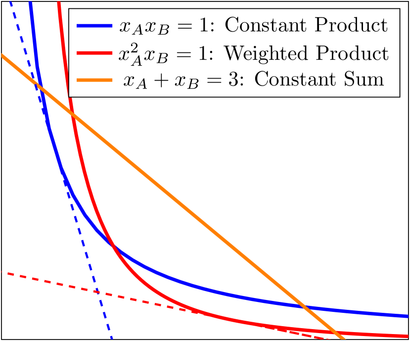
Figure 1. Examples of level sets of commonly studied CFMM trading functions. X-axis and Y-axis denote the amounts of assets A and B in the liquidity pool of the CFMM respectively. Examples of spot prices are illustrated by dashed lines. Where the trading function is differentiable, the negative slope of the tangent at a point gives the spot price (Definition 1.1).

We illustrate some examples of widely deployed and studied CFMM trading functions in Figure 1. We give some more examples in Appendix C.

1.1.2   Arrow Debreu Exchange Markets

An Arrow Debreu market (Arrow and Debreu, 1954) is used to model a pure exchange market, i.e., a market where a set of assets $\mathcal{A}$ are traded without a designated numeraire or “money”. Assets are fungible, divisible and freely disposable. Agents have quasi-concave and non-satiating utilities for the bundle of assets they consume and have an initial endowment of assets. All trades happen at the same prices implied by a valuation vector $\{{p_{A}}>0\}_{A\in\mathcal{A}}$, and asset amounts remain conserved.

1.1.3   Batch Exchanges

In a batch exchange, traders submit trade orders to an exchange operator, which gathers these orders into batches (typically with some temporal frequency, e.g. one batch per second) and then clears batches of orders subject to the constraints of the orders. Batch exchanges are sometimes modelled (Ramseyer et al., 2021; Walther, 2021) as instances of Arrow-Debreu exchange markets. The following are examples of order types that a batch exchange may support.

Definition 1.2 (Limit Sell Order).

A limit sell order $(A,B,k\in\mathbb{R}_{>0},r\in\mathbb{R}_{\geq 0})$, is an order to sell up to $k$ units of asset $A$ for as many units of asset $B$ as possible, subject to receiving a minimum price (the “limit price”) of $r$ $B$ per $A$.

This corresponds to a utility function $u(x)=rx_{A}+x_{B}$.

Definition 1.3 (Market Sell Order).

Limit sell orders with limit price of $0$ are market sell orders.

Definition 1.4 (Limit Buy Order).

A limit buy order is an order to purchase up to $k$ units of asset $A$ by selling as few units of asset $B$ as possible, subject to a maximum price of $r$ $B$ per unit $A$.

This corresponds to a utility function $u(x)=rx_{A}+\min(k,x_{B})$.

1.2. System Model

The design specifications are as follows:

1. A limit sell order can be submitted or removed any time before a cutoff for each next batch.

2. A CFMM participating in the batch exchange must submit its “state and trading function” to the exchange before a cutoff time for each next batch.

3. Between consecutive batches, the CFMMs may also be available for their standalone operation, but need to be unchanged after submitting their state and trading function to the batch exchange till the batch is executed.

We do not model the fee that the batch exchange operator and the CFMM charge. We believe that the axioms and properties of market solutions we study in this work are important also in the presence of trading fees.

1.3. Our Results

To our knowledge, this is the first paper to do an axiomatic and computational study of the important problem of augmenting batch exchanges with CFMMs. We design a batch exchange which supports limit sell orders (Definition 1.2) as traders and CFMMs as market makers.

1.3.1   Axioms

We give here (details are in §2) a minimal set of axioms for batch exchanges incorporating CFMMs. We require that a batch exchange neither burn nor mint any asset – asset amounts must be conserved (Axiom 1). We also impose the core fairness property of batch auctions that there exist asset valuations in equilibrium, and no market participant receives a better price than that implied by these valuations (Axiom 2). Together, Axioms 1 and 2 imply that all trades in a batch happen at the same batch prices (Observation 2). Further, as is standard in trading systems, we want that all limit orders receive a trade which is a “best response” to the batch prices (Axiom 3). This axiom ensures that a limit sell order fully executes when the batch price exceeds the limit price and is not executed at all when the batch price is less than the limit price. The axiom pertaining to CFMMs is their basic design principle that their trading function should not decrease due to a trade (Axiom 4).

Axioms 1, 2, and 3 are simply an articulation of the core properties of batch exchanges which we believe are well-accepted rules for designing exchange markets. Axiom 4 is a basic guarantee required by all CFMM deployments. These axioms are minimal and do not impose a particular solution. They allow a rich set of solution concepts with different economically useful properties, which is this paper’s core subject of study. We briefly discuss some solution concepts which carefully relax some axioms to expand the design space in §4.

We can now define a market equilibrium for batches with limit sell orders and CFMMs.

Definition 1.5 (Market Equilibrium).

For a batch trading in a set of assets $\mathcal{A}$, and market participants $i\in\mathcal{I}$ with initial endowments $\{x_{i,A}\geq 0\}_{i\in\mathcal{I},A\in\mathcal{A}},$ a market equilibrium consists of a set of valuations $\{{p_{A}}>0\}_{A\in\mathcal{A}}$ and allocations $\{z_{i,A}\geq 0\}_{i\in\mathcal{I},A\in\mathcal{A}}$ which satisfy Axioms 1, 2, 3, and 4 (asset conservation, uniform batch valuations, limit orders get a best-response trade, and the CFMM trading functions are non-decreasing).

We leverage existing results from the literature to obtain sufficient conditions for the existence of market equilibria. Multiple market equilibria may exist for any batch instance per Definition 1.5.

1.3.2   Desirable Properties of Batch Exchanges and Market Equilibria

We now define some desirable properties of market equilibria. These properties then guide us in designing algorithms for finding market equilibria which are economically more useful than some other market equilibria.

1. The first desirable property is Pareto optimality for the limit sell orders (Definition 3.1). An outcome of a mechanism is Pareto optimal if no agent can be made strictly better-off without making someone else strictly worse-off (Fudenberg and Tirole, 1991).

2. Another desirable property is price coherence (PC) of a group of CFMMs post-batch (Definition 3.4). PC is a necessary and sufficient condition for the participating CFMMs to be in a cyclic arbitrage-free state (Definition 3.3).

   A weaker condition than PC is preservation of price coherence (PPC), under which a group of participating CFMMs must be price-coherent post-batch if they were price-coherent pre-batch.

3. We also consider the property joint price discovery (JPD) (Definition 3.10) – a property strictly stronger than PC. JPD eradicates a form of arbitrage called parallel running (Definition 3.9).

   Observation 1.

   PPC is strictly weaker than PC, which is strictly weaker than JPD.

4. Another desirable property is locally computable response (LCR) (Definition 3.12) for the CFMMs. That is, the trade made by a CFMM in equilibrium is a deterministic function of only its trading function, its pre-batch state, and the batch asset valuations. If the exchange implements LCR for CFMMs, it provides predictability to the liquidity providers and can help them in doing a better risk-profit analysis and making a more informed decision about committing to a market-making strategy.

We also discuss a property called path independence (Definition 3.15) in § 3.5 motivated from the standalone operation of CFMMs for batches with a single limit order.

1.3.3   Achievability of Desirable Properties of Batch Exchanges

All results here are under the setup that Axioms 1-4 are required to be satisfied, that is the batch exchange computes a market equilibrium as a solution. We relax this only in § 4 where post-processing is allowed for the CFMMs after the market equilibrium. We start with two impossibility results regarding the achievability of certain desirable properties simultaneously.

Theorem 1.6.

A batch exchange cannot simultaneously guarantee Pareto optimality and preservation of price coherence (PPC).

Theorem 1.7.

A batch exchange cannot simultaneously guarantee a locally computable response (LCR) for CFMMs and Pareto optimality.

Recall that Pareto optimality is defined for the utilities of the limit orders, and PPC and LCR protect the interests of the CFMMs. These results shed light on an inherent tension between the interests of the CFMM and those of the limit orders. They also illustrate that the problem we study in this paper is non-trivial and nuanced.

We now turn to designing algorithms that find market equilibria with some of the desirable properties given above. For this, we adopt a viewpoint from the perspective of the CFMMs. Any deterministic algorithm for equilibrium computation can be described as a trading rule for a CFMM, a function which specifies the CFMM’s allocation, given all information of the batch instance.

Consider the following natural CFMM trading rule.

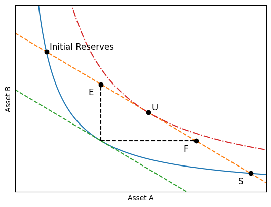
Figure 2. Examples of LCR CFMM trading rules. The axes are the CFMM’s reserves. The blue curve is a level curve of the CFMM trading function on which the initial state lies. The slope of the tangent to the level curve denotes the CFMM’s spot price. The slope of the dotted orange line is the negative of the batch price for this example. Here, the green and the orange lines have the same slopes.
Trading Rules S and U are per Definitions 1.10 and 1.8. Trading Rules E and F are inspired by the rebalancing strategy of Milionis et al. (2022) and are defined later in §4. The line segment between points E and F corresponds to the class of Strict-Surplus Trading Rules (Definition 4.5).

Definition 1.8 (Trading Rule U).

With its trading function as a pseudo-utility function, give the CFMM a pseudo-utility-maximizing bundle of assets subject to the asset valuations.

Under Assumption 1 on CFMM trading functions, the allocation under Trading Rule U is unique.

$$F_{U}(x,f,p)=\sup\limits_{z\in\{\hat{z}~{}|~{}p\cdot(\hat{z}-x)=0\}}f(z).$$

An illustration of Trading Rule U is in Figure 2. Notice that Trading Rule U satisfies LCR. That is, the CFMM’s allocation in equilibrium interacts with the rest of the batch only via the asset valuations $p$. When the CFMM demand under Trading Rule U satisfies an additional condition – Weak Gross Substitutability (WGS) – Trading Rule U in the batch exchange can be implemented by well-known algorithms for computing equilibria in Arrow Debreu markets, such as the Tâtonnement-based algorithm described in Codenotti et al. (2005a), or our convex program of §5. Apart from computational tractability, the simple Trading Rule U also has other desirable properties.

Theorem 1.9.

A batch exchange has JPD if and only if it implements Trading Rule U for all CFMMs.

By Observation 1, batch exchanges implementing Trading Rule U for all CFMMs also achieve PC. This implies that adopting Trading Rule U protects CFMMs from both cyclic arbitrage and parallel-running-based arbitrage. Trading Rule U has a natural interpretation that it treats CFMMs as utility-maximizing agents which may be normatively significant in many scenarios.

We also study Trading Rule S, which is applicable only for batches with 2-asset CFMMs.

Definition 1.10 (Trading Rule S).

Maximize the CFMM’s valuation-weighted trade size subject to the non-decreasing trading function constraint. Under Assumption 1, the allocation is unique.

$$F_{S}(x,f,p)=\sup\limits_{z\in\{\hat{z}~{}|~{}p\cdot(\hat{z}-x)=0;~{}f(\hat{z})\geq f(x)\}}\|p\cdot(z-x)\|_{1}.$$

An illustration of Trading Rule S is in Figure 2. Informally, it corresponds to trading “all the way” up to the point where the trading function non-decreasing constraint is tight. It always ends up on the same level curve of the trading function as the initial state. For the extreme sparse case of a single CFMM and a single limit order, Trading Rule S mimics a standalone CFMM, and therefore, in this case, a limit order based-trader does not strictly prefer trading “outside the batch” with the CFMM. Notice that Trading Rule S also satisfies LCR, i.e., it gives a CFMM’s “demand” as a response to asset valuations. All CFMM trading functions lead to a WGS demand under Trading Rule S, and as such, the equilibrium computation problem is computationally tractable (for example, once again, using the algorithm of Codenotti et al. (2005a) or the convex program of §5). This simple and intuitive solution concept has some more desirable properties in special cases of batch instances as we show here.

Although per Theorem 1.7, when guaranteeing LCR for all CFMMs, the batch exchange cannot guarantee Pareto optimal equilibria, it can nonetheless do so by using Trading Rule S for the special case of batches trading in only two assets when the CFMMs are price coherent pre-batch.

Theorem 1.11.

If the batch exchange trades in only two assets, and if the CFMMs in a batch are in a state of price coherence pre-batch, the equilibria obtained by algorithms implementing Trading Rule S for all CFMMs are Pareto optimal.

Trading Rule S is the only LCR CFMM trading rule with this property.

Theorem 1.11, in conjunction with the impossibility result of Theorem 1.7, shows how multi-asset batch exchanges pose much more analytical challenges than two-asset batch exchanges.

Trading Rule S, in general, does not satisfy PPC. However, this negative result is bypassed in batches with only “Concentrated Liquidity Constant Product” (CLCP) CFMMs (Definition 3.8), which is a class including the constant-sum and constant-product CFMMs.

Theorem 1.12.

CLCP is the unique class of CFMMs such that if all CFMMs in a batch belong to this class, then the market equilibria attained by batch exchanges implementing Trading Rule S for all CFMMs satisfy the preservation of price coherence.

This result uncovers a very interesting and useful fact about the class of CFMMs that are used extensively in practice and theory. While CLCP trading functions are hailed for their computational simplicity and universality (Adams et al., 2021), we establish the surprising fact here that they are also well-suited for integration with batch exchanges while using a very natural trading rule.

1.3.4   Results on Equilibrium Computation

Although tâtonnement-based algorithms can find market equilibria whenever agent demand functions are WGS, convex programs for computing market equilibria have led to an improved structural understanding of markets (such as the much-celebrated result of Eisenberg and Gale (1959)). Therefore, we develop a convex program (in §5) for computing market equilibria for markets with limit sell orders and 2-asset CFMMs that have a WGS demand under any given LCR CFMM trading rule. This program may be of independent interest – it makes progress on the open question of designing convex programs for nonlinear utility functions in Arrow Debreu exchange markets. Our program handles the case where agent utility functions are arbitrary quasi-concave functions of two assets, subject to the constraint that each agent’s demand function is WGS.

Theorem 1.13 (Informal).

The program with objective function COP and constraints C1, C2, and C3 is convex, and its solutions correspond to market equilibria (if one exists) when each agent trades in only two assets and their demand functions are WGS.

Our convex program is inspired by that of Devanur et al. (2016) for the case of linear utility functions. The proof is quite technical, but the intuition is easy to state – we develop a viewpoint from which CFMMs appear as an uncountable collection of infinitesimal limit sell offers. Unlike the analyses in Devanur et al. (2016) based on Lagrange multipliers, we have to go back to earlier techniques and directly apply Kakutani’s fixed point theorem.

When the density of this infinite collection of limit offers is a rational linear function, we prove that our convex program has rational solutions. This includes many classes of commonly used CFMMs, including the constant product CFMM when using Trading Rule U. On the flip side, we show that some CFMMs, for example those based on the Logarithmic Market Scoring Rule (LMSR) (Hanson, 2007), can force batches only to admit irrational equilibria when using Trading Rule U.

1.3.5   Solution Concepts Beyond Market Equilibria

A natural question is whether we can attain more of the desirable properties of §1.3.2 if we allow the CFMMs to do a post-processing step after their trade in the batch. The answer is yes but with a caveat. If the CFMMs have the option to alter their state post-batch, then they can always attain a state of price coherence, but this will have to violate the axiom of uniform valuations (Axiom 2). Further, we give a class of LCR trading rules – Strict-Surplus Trading Rules (Definition 4.5) – on 2-asset CFMMs with the following property:

In any market equilibrium where all CFMMs’ trades are per a Strict-Surplus Trading Rule, each CFMM has a surplus-capturing post-processing step, upon which they attain a state of JPD (Theorem 4.6).

This result opens up a new dimension to the solution space for our problem. Such multiple-step solutions concepts may provide a viable design in practice, but their economic implications must be further scrutinised in future research. More details on these results are in §4.

1.4. Related Work

In his seminal work, Kyle (1985) studied a model of a two-asset (a good and a money) batch auction where traders submit market orders to buy or sell the good. The market maker a priori declares a pricing rule that maps the excess demand for the good to a price. In contrast, we study a model where traders submit limit orders, and the market makers use a CFMM-based approach. A CFMM trading function, under LCR, can be considered a map from its trade size to a price for a given initial state. However, a CFMM is ‘automated’ in the sense that its pricing rule accounts for the liquidity provider’s ‘position’ in the good, which is captured in the initial state. Moreover, unlike Kyle (1985), we consider multi-asset batches and the case of potentially many market makers with their own CFMM trading functions.

Most closely related to our work in the blockchain space is the work of the company CoWSwap (Coincidence of Wants– Swap) (formerly known as Gnosis); their implementation details are provided in Walther (2021). Same as us, they study batches that incorporate CFMMs and trade in multiple assets. They take an optimization approach with various objectives, such as maximizing trade volume or maximizing trader utility. Their solutions are based on mixed integer programs and do not have runtime guarantees. In contrast, we take an axiomatic approach and propose polynomial time solutions for finding market equilibria with certain desirable properties.

Another blockchain-based system ZSwap designed by Penumbra (2023) considers batches of two assets only. They aggregate market orders in a batch and execute the excess demand with a CFMM per its constant function trading rule, subject to a maximum slippage tolerance.

Automated market-making strategies have been studied both in a cryptocurrency context (Angeris and Chitra, 2020) and in traditional exchanges (Glosten and Milgrom, 1985; Gerig and Michayluk, 2010; Kyle, 1985; Othman et al., 2013). CFMMs form a subclass of automated market-making. There has been extensive study on how the design of a CFMM trading function interacts with the economic incentives of those who invest in it (Evans et al., 2021; Capponi and Jia, 2021; Neuder et al., 2021; Fan et al., 2022; Cartea et al., 2022). Schlegel and Mamageishvili (2022); Frongillo et al. (2023); Park (2022) study the axiomatization of meaningful CFMM trading functions. Goyal et al. (2022); Milionis et al. (2023) develop frameworks for finding ‘optimal’ CFMM trading functions. However, this direction of work is orthogonal to the subject of study of this paper. We are interested only in the contract the CFMM-based trader enters into with the batch exchange operator. We capture a basic guarantee of this contract in Axiom 4.

Budish et al. (2015, 2014); Aquilina et al. (2022) study the economic performance of batch auctions between pairs of assets. The well-studied model of Arrow and Debreu (1954) forms the basis for multi-asset, pure exchange batch trading implementations (Jove et al., 2022; Walther, 2021). There are many classes of algorithms for (approximately or exactly) computing equilibria in Arrow-Debreu exchange markets, including iterative methods (or Tâtonnement) (Cole and Fleischer, 2008; Codenotti et al., 2005a; Codenotti et al., 2005b; Bei et al., 2019; Garg et al., 2019), convex programs for the case of linear utilities (Devanur et al., 2016; Jain, 2007; Nenakov and Primak, 1983; Cornet, 1989), convex program for Cobb-Douglas utilities (Curtis Eaves, 1985), and combinatorial algorithms (Jain et al., 2003; Devanur and Vazirani, 2003; Duan and Mehlhorn, 2015; Garg and Végh, 2019).

Most closely related to our work in this line is the convex program of Devanur et al. (2016), which also gives concise proof of the existence and rationality of equilibria. We generalize their program beyond linear utilities and include 2-asset WGS utility functions. The convex program of Nenakov and Primak (1983) (which was re-discovered by Jain (2007), since the original was in Russian) also goes beyond linear utilities but in an incomparable manner from ours. Their program can handle constant elasticity of substitution (CES) utilities for $\rho>0$ and Cobb-Douglas utilities on any number of assets but not the entire class of WGS utility functions. A precise characterization of the class of utility functions that their program can handle is unknown. Jain (2007) posed it as an open problem and gave several positive and negative examples. On the other hand, our program handles all WGS utility functions but only when each agent has utility for only two assets.

2. Axioms of Batch Exchanges with CFMMs

In this section, we give a set of axioms that specify minimal guarantees that a market solution must provide to the participants in a batch exchange.

2.1. Asset Conservation

Trading systems must not create or destroy any asset. This is equivalent to the “market-clearing” property of Arrow Debreu exchange market equilibria. Formally:

Axiom 1 (Asset Conservation).

Let exchange participants $i\in\mathcal{I}$ have endowments $\{x_{i,A}\}_{i\in\mathcal{I};A\in\mathcal{A}}$ and receive bundles $\{z_{i,A}\}_{i\in\mathcal{I};A\in\mathcal{A}}$. For each asset $A$, we must have $\sum_{i\in\mathcal{I}}x_{i,A}=\sum_{i\in\mathcal{I}}z_{i,A}.$

2.2. Uniform Valuations

The core fairness property of a batch trading scheme is that all orders in a batch trade at the same prices, and no trader gets an unfair advantage. For this, the batch exchange must compute valuations for all assets in a batch and ensure that no trader can get an allocation of a greater value than the value of their endowment per these valuations. Formally:

Axiom 2 (Uniform Valuations).

An equilibrium of a batch trading scheme has a shared market valuation $\{{p_{A}}>0\}$ for each asset $A\in\mathcal{A}$. Let batch exchange participants $i\in\mathcal{I}$ have endowments $\{x_{i,A}\}_{i\in\mathcal{I};A\in\mathcal{A}}$ and get allocated bundles $\{z_{i,A}\}_{i\in\mathcal{I};A\in\mathcal{A}}$. For each participant $i\in\mathcal{I}$, it must be the case that $p\cdot z_{i}\leq p\cdot x_{i}.$

Note that we do not require strict equality between $p\cdot z_{i}$ and $p\cdot x_{i}$ in the axiom; instead, we require that no market participant should get a price strictly better than the equilibrium asset valuations. However, in conjunction with asset conservation (Axiom 1), uniform valuation (Axiom 2) implies that this inequality needs to be strict in equilibrium.

Observation 2.

Axioms 1 and 2 imply that all trades in equilibrium in any asset pair $(A,B)\in\mathcal{A}^{2}$ happen at the same price, given by quotients of the asset valuations.

Proof.

Summing the inequalities of Axiom 2 over all participants, $\sum_{i\in\mathcal{I}}p\cdot z_{i}\leq p\cdot x_{i}.$ By asset conservation, $\sum_{i\in\mathcal{I}}z_{i}=\sum_{i\in\mathcal{I}}x_{i}$. Since all ${p_{A}}>0,$ all inequalities $p\cdot z_{i}\leq p\cdot x_{i}$ must be tight. ∎

One may envision a trading system allowing giving CFMMs a worse price than the limit orders to be able to execute some more limit orders. However, such a system will violate the asset conservation axiom and leave a surplus. This observation ensures that the $|\mathcal{A}|\choose 2$ exchange rates for each pair of assets are obtained from a vector of $|\mathcal{A}|$ asset valuations.

The existence of the valuation vector, which facilitates marker clearing, is not guaranteed for arbitrarily batch instances. However, we show in §5 that we can leverage the literature on Arrow Debreu markets to obtain the necessary conditions for the existence of market clearing valuations and corresponding allocations in our context.

2.3. Limit Sell Orders Make a Best Response

A basic guarantee of batch trading systems in the literature is that a limit sell order is executed in full when the batch price exceeds the limit price and is not executed when the batch price is less than the limit price. When the batch price equals the limit price, the limit order trades any amount between zero and its maximum amount.

Axiom 3 (Best response trade for limit orders).

The allocation received by a limit sell order maximizes its linear utility function subject to the market asset valuations.

2.4. CFMM Design Specification

The “constant function market maker” name may suggest that a CFMM shall trade from reserves $x$ to reserves $z$ only if $f(z)=f(x)$. One might consider encoding this strict equality condition as an axiom; however, real-world CFMM deployments only check the weaker condition that $f(z)\geq f(x)$ (uni, 2020). Keeping this flexibility allows us to have a much richer design space and is crucial to satisfy certain desirable properties of batch trading systems, as we shall see in the next section.

Axiom 4 (Non-decreasing CFMM trading function).

A CFMMs trading function does not decrease due to a trade in the batch, i.e., for a trade from state $x$ to $z$, we must have $f(z)\geq f(x)$.

Recall Definition 1.5 that any market equilibrium satisfies all Axioms 1, 2, 3, and 4.

3. Desirable Properties of Market Equilibria

Market equilibria may not be unique, so we turn now to study desirable properties of market equilibria, which will then guide our design of market equilibrium computation algorithms.

3.1. Pareto Optimality

Given the asset valuations in market equilibrium, the utility that a limit sell order receives is fixed under Axiom 3. However, some market equilibria may have asset valuations that provide a worse utility to the limit orders than other admissible market equilibria. The Pareto optimality of market equilibria is defined as follows.

Definition 3.1 (Pareto Optimal Market Equilibria).

For a batch instance, a market equilibrium $E$ is Pareto optimal if there does not exist another market equilibrium $E^{\prime}$ which Pareto dominates $E$ for the utility of the limit sell orders.

Note that in a market with only limit sell orders, all market equilibria are Pareto optimal – this property is lost if CFMMs also participate. There is no natural notion of the utility of a CFMM in our model, and since CFMMs are expected to charge trading fees (we do not model the fees in this paper), we define the Pareto optimality of market equilibrium for the utility of the limit orders only.

We illustrate with an example that multiple market equilibria may exist even for simple batch instances, and many of those may not be Pareto optimal.

Example 3.2.

Consider an instance of a batch exchange trading in assets $A$ and $B$, with a CFMM $f(x)=x_{A}x_{B},$ in the state $x_{A}=1,x_{B}=4,$ and a limit order $l=(A,B,1,1)$ i.e., for selling up to $1$ unit of $A$ for $B$ with a minimum price of $1$.

The set of market equilibria is given by the asset valuations $(p_{A}=r,p_{B}=1)$ for $r\in[1,2].$ The corresponding bundle that the limit order receives is $(z^{l}_{A}=0,z^{l}_{B}=r),$ and that the CFMM receives is $(z^{c}_{A}=2,z^{c}_{B}=4-r).$ The unique Pareto optimal market equilibrium corresponds to $r=2.$

We discussed Pareto optimality to safeguard the interests of the limit order traders. We now give desirable properties aimed at safeguarding the interests of the CFMM liquidity providers.

3.2. Price Coherence and Mitigating Cyclic Arbitrage

For a CFMM trading standalone (not in a batch exchange), its state changes only in response to trade requests and not directly in response to the prices of assets in the external market. When the external market prices change, the CFMM’s spot price is now “stale.” An arbitrageur can make a risk-free profit by buying from the CFMM some units of the asset whose relative price has increased on the external market and selling it there at the new (higher) price. The size of the trade to maximize the arbitrager’s profit can be computed by solving a convex program (Angeris et al., 2019). This optimal arbitrage trade leaves the CFMM’s spot price aligned with the external market’s price (Angeris and Chitra, 2020).

An arbitrage opportunity also arises when a group of CFMMs are mispriced with respect to each other. Towards this, we define “cyclic arbitrage”, which motivates important design considerations and properties we desire from market equilibria in batch exchanges.

Definition 3.3 (Cyclic Arbitrage of a Group of CFMMs).

A group of CFMMs $\mathcal{C}$ is in a state of cyclic arbitrage if it is possible to obtain a non-zero amount of any asset for free by trading with the group $\mathcal{C}$ simultaneously.

A state of cyclic arbitrage can arise, for example, when CFMMs operate in a batch exchange, and the system’s design does not eradicate this possibility. We define a related property on the spot prices of CFMMs, which provides a handle on the analysis of cyclic arbitrage.

Definition 3.4 (Price Coherence of a Group of CFMMs).

A group of CFMMs $\mathcal{C}$ has price coherence if there exists a set of asset valuations $\{q_{a}>0\}_{a\in\mathcal{A}}$ such that for each asset pair $(A,B)\in\mathcal{A}^{2},$ every CFMM $c\in\mathcal{C}$ that trades in asset pair $(A,B)$ has a spot price $\frac{q_{A}}{q_{B}}$ units of B per unit of A.

For a group of CFMMs, construct a graph with the CFMMs as nodes and an undirected edge between two nodes if they trade at least one common asset. If a set of CFMMs in a cycle of this graph (if one exists) does not have price coherence, then they are in a state with cyclic arbitrage – a trader can make a risk-free profit by carefully trading with this cycle of CFMMs. More precisely:

Proposition 3.5.

A group of CFMM are in a state of cyclic arbitrage if and only if they are not in a state of price coherence.

Proof.

Follows from the “no-arbitrage condition” of Angeris et al. (2022, pg. 121). ∎

The price coherence of a group of CFMMs motivates a related property for market equilibria.

Definition 3.6 (Price Coherence of Market Equilibria (PC)).

A batch exchange market equilibrium satisfies PC if the group of participating CFMMs have price coherence post-batch.

It is important for the liquidity providers of the CFMMs that cyclic arbitrage opportunities are not created by trading in the batch. We also define a weaker condition than price coherence for equilibrium computation algorithms, which may be more relevant in some circumstances.

Definition 3.7 (Preservation of Price Coherence (PPC)).

A batch exchange satisfies PPC if, for any batch instance with a group of CFMMs in a state of price coherence pre-batch, the equilibria computed by the exchange satisfy PC.

We now restate and prove Theorem 1.6.

Theorem 0 (1.6 restatement).

A batch exchange cannot simultaneously guarantee Pareto optimality and preservation of price coherence (PPC).

Proof.

Consider a batch instance trading in assets $\mathcal{A}=\{A,B\}.$ There are two CFMMs:

$C_{1}$ with trading function $f_{1}(x)=x_{A}x_{B}$ and pre-batch state $(x_{A}=1,x_{B}=2)$ with spot price $2$, and

$C_{2}$ with trading function $f_{2}(x)=x_{A}^{2}x_{B}$ and pre-batch state $(x_{A}=1,x_{B}=1)$ with spot price $2$.

There is a limit sell order $(A,B,1,1)$, i.e., to sell up to 1 unit of A for B for a price of at least 1.

The set of market equilibria is given by asset valuations $(p_{A}=r,p_{B}=1)$ for $r\in[1,(8+\sqrt{10})/9]$ and corresponding allocations.

The unique Pareto optimal market equilibrium corresponds to $r=(8+\sqrt{10})/9\approx 1.24.$ In this equilibrium, the post-batch spot price on CFMM $C_{1}$ is $\approx 0.769$ and that on CFMM $C_{2}$ is $\approx 0.748$. ∎

Although not possible to be guaranteed with Pareto optimality, PC can nonetheless be guaranteed by natural CFMM trading rules in batch exchanges. An example is Trading Rule U (recall Definition 1.8) – the result follows as a corollary of Theorem 1.9.

Recall that PPC is a weaker condition than PC. Although Trading Rule S (recall Definition 1.10) does not satisfy PPC in general, it does so when all CFMMs in the batch belong to a particular class of CFMMs, defined below.

Definition 3.8 (Concentrated Liquidity Constant Product (CLCP) Trading Functions).

A trading function in the CLCP class is $f(x)=(x_{A}+\hat{x}_{A})(x_{B}+\hat{x}_{B})$ for constants $\hat{x}_{A}>0,\hat{x}_{B}>0.$

This class of CFMMs allocates liquidity in a single interval of prices and implements the constant-product trading function in that interval. This price interval is $(\frac{\hat{x}_{B}^{2}}{K},\frac{K}{\hat{x}_{A}^{2}})$ for constant $K$ denoting the initial value of the CFMM trading function. This class includes, as special cases, the constant-product CFMM (Adams et al., 2020) (where the liquidity is spread to all prices, $0$ to $\infty$, by setting $\hat{x}_{A}=\hat{x}_{B}=0$) and the constant-sum CFMM (where the liquidity is concentrated at a single price point). Combinations of CLCP trading functions form the basis of the widely successful decentralized exchange protocol Uniswap V3 (Adams et al., 2021). CLCP trading functions have the following interesting property.

Theorem 0 (1.12 restatement).

CLCP is the unique class of CFMMs such that if all CFMMs in a batch belong to this class, then the market equilibria attained by batch exchanges implementing Trading Rule S for all CFMMs satisfy the preservation of price coherence.

Proof.

Denote the asset valuations which give the initial spot prices of the CFMMs by $\{q_{a}\}_{a\in\mathcal{A}}.$ These exist by pre-batch price coherence. Denote the batch equilibrium asset valuations by $\{p_{a}\}_{a\in\mathcal{A}}$ and the asset valuations which give the post-batch spot prices of the CFMMs by $\{\hat{q}_{a}\}_{a\in\mathcal{A}}.$ These exist by PPC. Since each CFMM here trades in only two assets (Trading Rule S is defined only for 2-asset CFMMs), its initial spot price is $q_{AB}=q_{A}/q_{B}$ for assets $A$ and $B$ that it trades. Similarly, denote the batch price in $A$ and $B$ by $p_{AB}.$

For a given CFMM trading function, recall that Trading Rule S gives a map $F_{S}$ (Definition 1.10) from the initial state and the batch asset valuations to the final state. Observe that this map depends on $\{p_{a}\}_{a\in\mathcal{A}}$ only via the batch price $p_{AB}.$ Under the strict quasi-concavity of the CFMM trading function, if the CFMM trading function value is invariant, there is an injective map from the CFMM state to its spot price. Since the CFMM trading function value is invariant under Trading Rule S, we can represent Trading Rule S as a map from the initial spot price and batch price to the final spot price. Denote this map for trading function $f$ by $g_{f}(q_{AB},p_{AB})\rightarrow\hat{q}_{AB}.$

Here, we give properties that the map $g_{f}(\cdot,\cdot)$ must satisfy.

1. Reflexive. That is, $g_{f}(\rho,\rho)=\rho$ for all $\rho\in[0,\infty).$ This is required since the CFMM makes no trade when the batch price equals the spot price, and hence the post-batch spot price should equal the initial spot price.

2. Involution on the Spot Price. That is, $g_{f}(q,p)=\hat{q}\implies g_{f}(\hat{q},p)=q$ for all $q,p,\hat{q}\in[0,\infty).$ This is because, under Trading Rule S, the CFMM returns to the initial state after two consecutive batches if the batch price is the same in both batches.

3. PPC. For a group of CFMMs, construct a graph with the CFMMs as nodes and an undirected edge between two nodes if they trade at least one common asset. For any cycle $\mathbb{C}$ of CFMMs in this graph, see that $\prod_{i\in\mathbb{C}}p_{A_{i}B_{i}}=1$ by arbitrage-freeness of batch valuations (here CFMM $i$ trades in asset $A_{i}$ and $B_{i}$, $A_{i+1}=B_{i},$ and $B_{|\mathbb{C}|}=A_{1}$). Also $\prod_{i\in\mathbb{C}}q_{A_{i}B_{i}}=1$ by pre-batch PC. PPC requires that $\prod_{i\in\mathbb{C}}g_{f_{i}}(q_{A_{i}B_{i}},p_{A_{i}B_{i}})=1.$

From basic functional analysis, we obtain that the only differentiable functions that satisfy these conditions are $g_{f}(q,p)=q$ and $g_{f}(q,p)=\frac{p^{2}}{q}.$

The case of $g_{f}(q,p)=q$ corresponds to the constant sum CFMM whose spot price is invariant to the CFMM state. Observe that this CFMM is in the CLCP class (Definition 3.8) and corresponds the case where the liquidity is concentrated at one price.

We now solve for the trading function corresponding to $g_{f}(q,p)=\frac{p^{2}}{q}.$

Let a CFMM trade in assets $A$ and $B$, and its reserves in each asset be $x_{A}$ and $x_{B}$. When CFMM trading function value $f(x)$ is invariant, it gives an injective map from $A$ in the reserves to $B$ in the reserves. Denote this map by $B_{f}(x_{A})$ for a fixed level curve of the CFMM trading function $f$. In this notation, the spot price of the CFMM is $\frac{dB_{f}}{dx_{A}}.$

For two points on a level curve, $(x_{A0},x_{B0})$ and $(x_{A1},x_{B1}),$ the condition $g_{f}(q,p)=\frac{p^{2}}{q}$ translates to

(1) $$\frac{dB_{f}}{dx_{A}}\bigg{\rvert}_{x_{A0}}\cdot\frac{dB_{f}}{dx_{A}}\bigg{\rvert}_{x_{A1}}=\left(\frac{x_{B1}-x_{B0}}{x_{A1}-x_{A0}}\right)^{2}$$

Taking the point $(x_{A0},x_{B0})$ as fixed, denoting $\frac{dB_{f}}{dx_{A}}\Big{\rvert}_{x_{A0}}$ by constant $c,$ and solving the differential equation yields the following indefinite integrals.

(2) $$c\int\frac{dB_{f}}{(x_{B1}-x_{B0})^{2}}=\int\frac{dx_{A}}{(x_{A1}-x_{A0})^{2}}$$

Further solving gives

(3) $$\frac{c}{(x_{B}-x_{B0})}=\frac{1}{(x_{A}-x_{A0})}+c_{1}$$

where $c_{1}$ is the constant of integration. For $x_{B}\neq x_{B0}$ and $x_{A}\neq x_{A0}:$

(4) $$c(x_{A}-x_{A0})=(x_{B}-x_{B0})+c_{1}(x_{A}-x_{A0})(x_{B}-x_{B0})$$

Upon rearrangement of the terms, this yields the CLCP trading function form. In case the CFMM runs out of an asset, the spot price for selling that asset is $\infty$ for a CLCP trading function – using this value in the PC equation ensures that the result continues to hold. ∎

3.3. Joint Price Discovery and Mitigating Parallel Running

We motivated PC and PPC, intending to ensure that the group of CFMMs participating in the batch exchange do not end up in a state of cyclic arbitrage. However, the problem of arbitrage in financial systems is not limited to the trades that can be made with a group of CFMMs.

Here we study another form of an arbitrage strategy.

Definition 3.9 (Parallel Running).

For a batch instance, a parallel running arbitrage opportunity exists if for any real numbers $a,b>0$ and any assets $A,B\in\mathcal{A},$ a trader can sell $a$ units of asset $A$ in exchange for $b$ units of asset $B$ in the batch and, can then obtain $a$ units of asset $A$ in exchange for $\hat{b}<b$ units of asset $b$ by trading with the participating CFMMs post-batch.

Parallel running is a similar concept to front running, which corresponds to making a trade based on advanced knowledge of future orders. By definition, precisely identifying parallel running opportunities requires knowledge of all the other batch participants and the equilibrium computation algorithm. However, estimating the chances and magnitudes of such opportunities with only partial information may be possible – we leave this investigation for future work. We show here that we can design equilibrium computation algorithms that eradicate all parallel running opportunities, even if the arbitrager has perfect information of the batch.

First, we describe a property of market equilibria.

Definition 3.10 (Joint Price Discovery (JPD)).

Let group $\mathcal{C}$ of CFMMs participate in a batch. A market equilibrium with asset valuations $\{p_{a}>0\}_{a\in\mathcal{A}}$ satisfies JPD if for each asset pair $(A,B)\in\mathcal{A}^{2},$ every CFMM $c\in\mathcal{C}$ that trades in pair $(A,B)$ has a post-batch spot price $\frac{p_{A}}{p_{B}}$ units of B per unit of A.

Observe that JPD is a special case of PC. The following result establishes its importance as a defence against parallel running.

Lemma 3.11.

Joint price discovery (JPD) makes parallel running impossible.

Proof.

See that in equilibrium, each order in the batch executes at the batch prices given by the ratios of asset valuations $\{p_{a}>0\}_{a\in\mathcal{A}}.$ By quasi-concavity of CFMM trading function $f$, for any trade, the price obtained is no better than the spot price. By JPD, the spot price is equal to the batch price, so parallel running is impossible. ∎

We show in Appendix B that for a reasonable regularity condition “split invariance” on equilibrium computation algorithms (in Definition B.2) and for “large” batch instances (as in Definition B.1), JPD is a necessary condition to eradicate parallel running in batch exchanges.

Beyond its desirable properties, JPD implies a natural CFMM trading rule. Towards this, we here restate and prove Theorem 1.9.

Theorem 0 (1.9 restatement).

A batch exchange has JPD if and only if it implements Trading Rule U for all CFMMs.

Proof.

The CFMM trading function $f$ is strictly quasi-concave. Thus, to maximize $f$ on a hyperplane (as in Trading Rule U) is to find the point where the gradient of $f$ is normal to the hyperplane. This point is unique under Assumption 1. Since the gradient of $f$ at a point is equal to the spot price at said point (up to rescaling), setting the spot prices equal to the batch prices corresponds to Trading Rule U. ∎

JPD has another advantage beyond mitigating parallel running. Previous work (Economides and Schwartz, 2001; Schwartz, 2012) suggests that batch exchanges may emerge as major trading venues for the price discovery of assets. If this prediction is realized, then it will be vital for the CFMMs to have a spot price in lockstep with the price offered on the batch exchange. In a way, CFMMs shall achieve price discovery for “free” by trading in a batch exchange which implements JPD-ensuring market equilibria, which otherwise (in their standalone operation) comes at the cost of arbitrage or “loss-vs-rebalancing” as Milionis et al. (2022) term it. A thorough analysis of the economic incentives of CFMM liquidity providers to participate in batch exchanges is the subject of future research. We now study another property aimed at safeguarding the CFMMs.

3.4. Locally Computable Response for CFMMs

It is often important for agents to have some predictability in their trade in a batch, subject to the batch prices. While this is guaranteed for limit orders axiomatically (Axiom 3), it would also be good for liquidity providers who invest their capital in CFMMs for market making.

Definition 3.12 (Locally Computable Response (LCR) CFMM Trading Rule).

A CFMM’s trading rule in a batch exchange satisfies LCR if it is a map $F(x,f,p)\rightarrow z,$ where $\{x_{a}\}_{a\in\mathcal{A}}$ is the pre-batch CFMM state, $f$ is its trading function, and $\{p_{a}\}_{a\in\mathcal{A}}$ is a set of equilibrium asset valuations. The output $\{z_{a}\}_{a\in\mathcal{A}}$ is the post-batch CFMM state.

Further, $F(x,f,p)$ must be invariant under rescaling of $p$.

LCR provides predictability to liquidity providers and makes participation more lucrative (apart from the fees they charge, which are not considered in our model). However, as with other desirable properties, we lose some design space if we impose LCR for CFMMs. For example, we have the impossibility result of Theorem 3.14, which uses Definition 3.13.

Definition 3.13.

The price-weighted trade volume of a limit sell order selling A for B is $p_{A}(x_{A}-z_{A})+p_{B}(z_{B}-x_{B})$ where $x$ and $z$ are their endowment and equilibrium allocation, respectively, and $p$ are the equilibrium asset valuations.

Theorem 3.14.

No batch exchange satisfying LCR for CFMMs can guarantee to find a market equilibrium that maximizes the sum of the price-weighted trade volumes of all limit sell orders.

Proof.

Consider a batch exchange with a single CFMM with trading function $f(x)=x_{A}x_{B}$ and pre-batch state $x_{A}=1,x_{B}=4.$ We study two batch instances with this CFMM:

1. There is one limit sell order $(A,B,3,1)$ i.e., for selling up to $3$ units of $A$ for a minimum price of $1$ $B$ per $A$. All equilibria have the same (up to rescaling) asset valuations: $p_{A}=p_{B}=1$.

   The “price-weighted trade volume of limit orders” is maximized by the equilibrium at which the CFMM buys $3$ units of $A$ from the limit order.

2. There is one limit sell order $(A,B,3,1)$ and another limit sell order $(B,A,3,1).$ All equilibria have the same (up to rescaling) asset valuations: $p_{A}=p_{B}=1$.

   The “price-weighted trade volume of limit orders” is maximized by the equilibrium at which the CFMM makes no trades.

Since the equilibrium asset valuations are the same in the two instances, any LCR trading rule for the CFMM cannot distinguish between the two instances and cannot optimize for the price-weighted trade volume of limit orders. ∎

Walther (2021) gives a mixed-integer program for the problem of finding a market equilibrium that maximizes the price-weighted trade volume of limit orders. Their algorithm has no runtime guarantees. Finding polynomial-time algorithms for this objective or showing that none exist is an interesting open problem. Also, recall the impossibility result of Theorem 1.7. We prove it here.

Theorem 0 (1.7 Restatement).

A batch exchange cannot simultaneously guarantee a locally computable response (LCR) for CFMMs and Pareto optimality.

Proof.

First consider the case of LCR CFMM trading rules which, for some starting state $x,$ trading function $f,$ and batch valuations $p,$ demand an allocation $z$ strictly “above the curve”, i.e., $f(z)>f(x).$ Such a CFMM trading rule will clearly not lead to a Pareto optimal equilibrium. Consider a batch with one market sell order selling $A$ for $B,$ and a CFMM trading in a set of assets $\mathcal{A}$ which includes $A$ and $B$. If, in equilibrium, the CFMM’s allocation $z$ satisfies $f(z)>f(x),$ then, by the strict quasiconcavity of $f,$ there exists an alternate equilibrium under which the CFMM’s allocation is $z^{\prime}$ where $z^{\prime}_{B}<z_{B},$ $f(z^{\prime})=f(x)$ (hence satisfying Axiom 4), and $\{z^{\prime}_{a}\}_{a\in\mathcal{A}\setminus B}=\{z_{a}\}_{a\in\mathcal{A}\setminus B}.$ In this equilibrium, the limit order gets strictly more units of assets B and is, therefore, a Pareto improvement.

Now, consider the case of LCR CFMM trading rules which, for all starting states $x,$ trading functions $f,$ and batch valuations $p,$ demand an allocation $z$ “on the curve”, i.e., $f(z)=f(x).$ For two-asset CFMMs, this leaves only two possibilities (by strict quasi-concavity of trading function $f$), either the CFMM makes no trade (i.e., $z$ = $x$) or the CFMM demands an allocation $z$ such that $z=\sup\limits_{z~{}\in~{}\{\hat{z}|p\cdot(\hat{z}-x)~{}=~{}0;~{}f(\hat{z})~{}\geq~{}f(x)\}}\|p\cdot~{}(z-x)~{}\|_{1}$. Recall that this corresponds to Trading Rule S. We consider both these cases.

1. There exists a CFMM $C$ in the batch with an LCR trading rule which, for some starting state $x,$ trading function $f,$ and batch valuations $p$ (not equal to the CFMM spot price), demands an allocation $z$, where $z=x$ (that is, makes no trade).

   Say CFMM $C$ trades in assets $A$ and $B$. Consider a batch where no other group of CFMMs together trade in both $A$ and $B$. There exists a batch instance with a market sell order for $a>0$ units of asset $A$ for $B$. The equilibrium under the above-stated LCR is sub-optimal for the limit order since it would have a higher utility on receiving any non-zero amount of $B$.

2. Consider a case where all CFMMs in the batch are two-asset CFMMs, and they follow the LCR Trading Rule S. For this case, we have the following example with two CFMMs and two limit sell orders.

   CFMM $C_{1}$ trades in assets $A$ and $B,$ uses the trading function $f(x)=x_{A}x_{B}$ and has a starting state $(x_{A}=1,x_{B}=4).$

   CFMM $C_{2}$ trades in assets $B$ and $D,$ uses the trading function $f(x)=x_{B}x_{D}$ and has a starting state $(x_{B}=1,x_{D}=4).$

   Limit order $L_{1}=(A,D,3,1)$ i.e., to sell up to $3$ units of $A$ for $D$ at a minimum price of $1$ D per A.

   Limit order $L_{2}=(A,B,1,1.5).$

   On using Trading Rule S for both CFMMs, a market equilibrium $E$ has asset valuations $p_{A}=p_{B}=p_{D}=1$. CFMM $C_{1}$ buys $3$ units of $A,$ sells $3$ units of $B,$ and ends up in a state of $x_{A}=4$ and $x_{B}=1$. CFMM $C_{2}$ buys $3$ units of $B,$ sells $3$ units of $D,$ and ends up in a state of $x_{B}=4$ and $x_{D}=1$. Limit order $L_{1}$ trades in full and limit order $L_{2}$ does not trade.

   Another market equilibrium, $\hat{E}$, has asset valuations $p_{A}=2;p_{B}=1;p_{D}=2$.

   CFMM $C_{1}$ buys $1$ unit of $A$ and sells $2$ units of $B$. CFMM $C_{2}$ makes no trades. Limit order $L_{1}$ makes no trade and limit order $L_{2}$ trades in full (sells $1$ unit of $A$ for $2$ units of $B$). The utility of $L_{1}$ is the same in $E$ and $\hat{E}$, whereas that of $L_{2}$ is strictly better in $\hat{E}$. Therefore market equilibrium $\hat{E}$ is a Pareto improvement over $E$. ∎

These negative results illuminate the fundamental trade-offs that a batch exchnage must operate under. However we are able to obtain positive results in an important special case. We restate and prove Theorem 1.11.

Theorem 0 (1.11 Restatement).

If the batch exchange trades in only two assets, and if the CFMMs in a batch are in a state of price coherence pre-batch, the equilibria obtained by algorithms implementing Trading Rule S for all CFMMs are Pareto optimal.

Trading Rule S is the only LCR CFMM trading rule with this property.

Proof.

Let assets $A$ and $B$ be traded on the exchange. Denote a market equilibrium obtained by implementing Trading Rule S for all CFMMs by $E$. By pre-batch price coherence, CFMMs either all sell $B$ or all sell $A$ in equilibrium. The CFMMs sell $B$ in $E$ without the loss of generality.

An improvement in the utility of the limit orders selling $A$ can be made only by making $B$ cheaper relative to $A$. For higher utility, the limit orders selling $A$ consume strictly more $B$ than in equilibrium $E$. On the other hand, the limit orders selling $B$ sell strictly fewer $B.$ However, the CFMMs, all of whom are selling $B$ in $E$, cannot sell any more of $B$ at a lower price by the quasi-concavity of the trading function $f$ and the fact that the CFMM is “on the curve” in Trading Rule S. Therefore such a utility improving market equilibrium is not possible.

An improvement in the utility of the limit orders selling $B$ can be made only by making $B$ costlier relative to $A$. However, in equilibrium $E$, some limit orders are buying $B$ (since the CFMMs all sell $B$), and making $B$ costlier will strictly decrease their utility.

We now show that Trading Rule S is the only LCR CFMM trading rule with this property, with a simple example. Consider a batch instance with a market sell order for selling asset $A$ for $B$. If for some initial state $x$ and trading function $f$, the batch exchange does not implement Trading Rule $S$, then it provides strictly fewer units of $B$ to the limit order than under Trading Rule $S$ and is therefore not Pareto optimal. ∎

3.5. Path Independence

We here discuss a property of the batch exchange (and not of market equilibria like the previous properties), defined when there is a single limit order-based trader. Blockchain systems often have restricted throughput capabilities, and it is important to design mechanisms which do not incentivize traders to submit multiple small orders instead of a single big order. Towards this, we define the path-independence property, which is inspired by the standalone operation of CFMMs.

Definition 3.15 (Path Independence).

An arbitrary group of CFMMs $\mathcal{C}$ participates in two consecutive batches and does not modify between the batches. Suppose a single trader exists and wants to sell some units of an asset $A\in\mathcal{A}$ in exchange for asset $B\in\mathcal{A}$ via market sell orders (that is, limit sell orders with limit price zero).

In a path-independent batch exchange, the amount of asset $B$ they receive on splitting the units of $A$ they sell into the two batches is independent of the split.

This definition trivially extends to multiple batches and not just two. Standalone CFMMs satisfy path independence (Angeris and Chitra, 2020). However, it is surprisingly difficult to satisfy in batch exchanges, except for a narrow case of Theorem 3.16. We restate and prove Theorem 3.16 here.

Theorem 3.16.

Batch exchanges with Trading Rule S for CFMMs satisfy path independence when there is only one CFMM in the batch.

Proof.

The CFMM, under Trading Rule S, trades “on the curve.” That is, $f(z)=f(x)$ where $x$ and $z$ are its pre-batch and post-batch states, respectively. For any amount of $A$ that the market order trader sells, the amount of $B$ in the CFMM is specified by the trading function preservation and therefore the amount of $B$ that the trader receives is also only a function of the net amount of $A$ sold by the trader.∎

The path independence property, although defined in a restricted setup, provides a distinction between Trading Rules U and S. Even in the simple setup of a single CFMM and a single limit-order-based trader, batch exchanges implementing Trading Rule U do not satisfy path independence, as shown in the following example.

Example 3.17 (Trading Rule U does not satisfy path independence with one CFMM).

Consider a batch instance with a single CFMM with trading function $f(x)=x_{A}x_{B}$ and pre-batch state $x_{A}=1,x_{B}=4.$

If a trader submits a market sell order for 2 units of $A,$ they receive $1.6$ units of $B.$ (See that the new CFMM state: $x_{A}=3,x_{B}=2.4$, has a spot price of $0.8$ B per A, which matches the batch price offered).

If the same trader first submits a market sell order for $1$ unit of $A,$ they receive $4/3$ units of B for it. The new CFMM state is $x_{A}=2,x_{B}=8/3$. Now if they make another market sell order for $1$ unit of $A,$ they receive $2/3$ units of $B$ for it, with the final CFMM state of $x_{A}=3,x_{B}=2$. The overall trade is $2$ A for $2$ B, which is strictly better than what they received on trading in full in one go.

Although simple and intuitive in the case of 2-asset batches, the path independence property is surprisingly difficult to satisfy. Even Trading Rule S does not satisfy it when more than one CFMMs are present, even if the CFMMs are price-coherent pre-batch, as in the following example.

Example 3.18.

CFMM $C_{1}$ trades in assets $A$ and $B,$ uses the trading function $f(x)=x_{A}x_{B}$ and has a starting state $(x_{A}=10,x_{B}=1).$

CFMM $C_{2}$ also trades in assets $A$ and $B,$ uses the trading function $f(x)=x_{A}+10x_{B}$ and has a starting state $(x_{A}=10,x_{B}=0).$

If a trader sells 1 B, they receive 10 A; CFMM $C_{1}$ makes no trade, and CFMM $C_{2}$ trades to state $(x_{A}=0,x_{B}=1)$. Then, if they sell another B, CFMM $C_{1}$ trades to final state $(x_{A}=5,x_{B}=2)$ and CFMM $C_{2}$ makes no trade. Overall the trader receives 15 A for 2 B.

But if they sell 2B together, the price is (3/20) A per B; CFMM $C_{1}$ trades to final state $(x_{A}=1.5,x_{B}=0)$ and CFMM $C_{2}$ trades to final state $(x_{A}=20/3,x_{B}=3/2)$. The trader receives 40/3 A for 2 B.

This example shows that path independence is at a conflict with the interests of the CFMM, and it can be satisfied only in special cases.

We now move on to solution concepts that allow the CFMMs for an extra step after the batch. We show that doing so carefully can expand our design space in interesting and useful ways.

4. Beyond Market Equilibria Solutions

Here we study the case where the CFMMs are capable of post-processing their state after the batch trade and before being open to standalone operation. For example, CFMMs can restore price coherence through a careful post-processing step. This can, for example, be facilitated by the batch operator. A simple method is to run a “phantom batch” with no limit orders and an equilibrium computation algorithm implementing Trading Rule U for all CFMMs. By doing so, the batch exchange may retain some desirable properties of solutions that do not guarantee PC in the main batch (for example Trading Rule S), and then also attain PC before subsequent operations by running the phantom batch. This 2-step solution seems to violate our impossibility result of Theorem 1.6, but it does not! This solution violates the axiom of uniform valuations (Axiom 2) since the asset valuations in the phantom batch may deviate from those in the main batch.

We showed here how participating CFMMs in a state of cyclic arbitrage can jointly post-process from an arbitrary initial state to reach a price coherent state. Importantly, this operation can be performed after adopting any equilibrium computation algorithm in the main batch. Our second result in this section is even more interesting. We now study a class of locally computable CFMM trading rules with the following property. Batches where the equilibrium computation algorithm implements a trading rule from this class for all CFMMs, assure that the CFMMs can locally post-process and attain a state of JPD. Importantly, this local post-processing strategy does not entail making a trade or changing the CFMM trading function, it simply entails capturing a part of the CFMM reserves as ‘profit’ and removing it from the market-making pool. In the process, the CFMM reaches a state where the value of the trading function is equal to its pre-batch value. The caveat is that this 2-step process violates asset conservation since assets are effectively removed from the system at the end of it. For this, we first define Trading Rules E and F.

For a standalone CFMM trading in two assets A and B, under Assumption 1, there is an injective map from the spot price to the CFMM state. Motivated by the ‘rebalancing’ strategy of Milionis et al. (2022), a CFMM trading rule can be designed to buy as much of asset A as it would hold ‘on the curve’ when the spot price equals the batch price.

Definition 4.1.

For the initial CFMM state $x$ and its trading function $f$, denote the map from the spot price $p$ to the amount of asset A in the CFMM state by $\mathbb{A}(x,f,p),$ i.e.,

$$\mathbb{A}(x,f,p)=\{z_{A}|f(z)=f(x);\frac{\partial f}{\partial x_{A}}(z)/\frac{\partial f}{\partial x_{B}}(z)=p\}.$$

Definition 4.2.

For the initial CFMM state $x$ and its trading function $f$, denote the map from the spot price $p$ to the amount of asset B in the CFMM state by $\mathbb{B}(x,f,p),$ i.e.,

$$\mathbb{B}(x,f,p)=\{z_{B}|f(z)=f(x);\frac{\partial f}{\partial x_{A}}(z)/\frac{\partial f}{\partial x_{B}}(z)=p\}.$$

For strictly quasiconcave CFMM trading functions, $\mathbb{A}(x,f,p)$ and $\mathbb{B}(x,f,p)$ are singleton. For non-strict quasiconcave CFMM trading functions, we can use any arbitrary elements of the sets defined above for the rest of the discussion. This enables us to define two CFMM trading rules.

Definition 4.3 (Trading Rule E).

The allocation obtained by a CFMM in market equilibrium is such that it gets as much A as it holds on the intital level curve of $f$ when the spot price equals the batch price. That is: $F_{E}(x,f,p)=z$ where $z_{A}=\mathbb{A}(x,f,p_{A}/p_{B})$ and $z_{B}=(1/p_{B})(x_{A}p_{A}+x_{B}p_{B}-\mathbb{A}(x,f,p_{A}/p_{B})p_{A}).$

In a similar vein, we also have Trading Rule F.

Definition 4.4 (Trading Rule F).

The allocation obtained by a CFMM in market equilibrium is such that it gets as much B as it holds on the intital level curve of $f$ when the spot price equals the batch price. That is: $F_{F}(x,f,p)=z$ where $z_{A}=(1/p_{A})(x_{A}p_{A}+x_{B}p_{B}-\mathbb{B}(x,f,p_{A}/p_{B})p_{B})$ and $z_{B}=\mathbb{B}(x,f,p_{A}/p_{B}).$

Observe that both Trading Rules E and F satisfy LCR. We illustrate these trading rules in Figure 2. We define a class of LCR trading rules for 2-asset CFMMs – Strict-Surplus Trading Rules – as a parameterized interpolation between Trading Rules E and F.

Definition 4.5 (Strict-Surplus Trading Rules).

The allocation obtained by a CFMM in market equilibrium under Strict-Surplus Trading Rule with parameter $\theta\in[0,1]$ is $F_{\theta}(x,f,p)=z$ where $z_{A}=\theta\mathbb{A}(x,f,p_{A}/p_{B})+(1-\theta)(1/p_{A})(x_{A}p_{A}+x_{B}p_{B}-\mathbb{B}(x,f,p_{A}/p_{B})p_{B})$ and,
$z_{B}=\theta(1/p_{B})(x_{A}p_{A}+x_{B}p_{B}-\mathbb{A}(x,f,p_{A}/p_{B})p_{A})+(1-\theta)\mathbb{B}(x,f,p_{A}/p_{B}).$

Strict-Surplus Trading Rules have a special property captured in the following theorem.

Theorem 4.6.

A CFMM with trading function $f$ and initial state $x$ trading in assets A and B with a Strict-Surplus Trading Rule with parameter $\theta$ can, post-batch, extract a non-negative surplus $e$ where

$e_{A}=(1-\theta)(x_{A}-\mathbb{A}(x,f,p_{A}/p_{B})+(x_{B}-\mathbb{B}(x,f,p_{A}/p_{B}))p_{B}/p_{A}),$ and

$e_{B}=\theta((x_{A}-\mathbb{A}(x,f,p_{A}/p_{B}))p_{A}/p_{B}+x_{B}-\mathbb{B}(x,f,p_{A}/p_{B})),$

and reach a state $z^{\prime}$ where $z^{\prime}_{A}=\mathbb{A}(x,f,p_{A}/p_{B})$ and $z^{\prime}_{B}=\mathbb{B}(x,f,p_{A}/p_{B})$.

After surplus extraction, the trading function becomes equal to its pre-batch value, i.e., $f(z^{\prime})=f(x)$.

If all CFMMs in the batch extract their respective surplus, the final state satisfies JPD.

Proof.

Follows from Definitions 4.1, 4.2, and 4.5. ∎

This result augments our design space in a significant manner if the batch exchange believes that JPD is important but wants to try solution concepts other than Trading Rule U. Informally, Trading Rule F, which is a Strict Surplus trading rule, may provide more liquidity to the market than Trading Rule U in some cases (observe from Fig 2 that in this example, Trading Rule F implies a larger trade for the CFMM than Trading Rule U at the same batch price).

5. A Convex Program for 2-asset WGS Demands

Here we give a convex program that computes market equilibria in batch exchanges that incorporate CFMMs that trade between two assets and use locally-computable trading rules that satisfy WGS. Alternatively, this program computes equilibria in Arrow-Debreu exchange markets where every agent’s demand response satisfies WGS, and every agent has utility in only two assets. The program is based on the convex program of Devanur et al. (Devanur et al., 2016) for linear exchange markets.

The key observation is that 2-asset CFMMs satisfying WGS can be viewed as (uncountable) collections of agents with linear utilities and infinitesimal endowments. This correspondence lets us replace a summation over agents with an integral over this collection of agents. However, proving the correctness of our program requires direct analysis of the objective instead of the argument based on Lagrange multipliers used in (Devanur et al., 2016). The objective is smooth on the feasible region, and gradients are easily computable for many natural CFMMs.

5.1. From a Demand Function to a Continuum of Limit Orders

Suppose that a batch participant is only interested in two assets $A$ and $B$. We first give a viewpoint that corresponds such an agent to a continuum of exchange market agents with linear utility functions that trade between $A$ and $B$. Under LCR, such an agent’s demand function can only depend on the price between the two assets (that is, $r_{AB}=\frac{p_{A}}{p_{B}}$). We can therefore define a function $S_{A}(\cdot)$ that gives, for any price $r_{AB}$, the amount of asset $A$ that the agent sells (in net, relative to its initial endowment).

Definition 5.1 (Supply).

Consider a batch participant with endowment $x$ that only trades between assets $A$ and $B$. The Supply of the participant of asset $A$ at exchange rate $r_{AB}>0$ is the set $S_{A}(r_{AB})=\{\max(0,x_{A}-z_{A})\}$, where $z$ is an amount of $A$ that could be held by the agent after a batch is settled.

For agents maximizing a utility function (i.e. limit sell orders), $z$ ranges over utility-maximizing allocations, and for a CFMM using some trading rule, $z$ is the allocation specified by the trading rule.

A supply function $S_{A}(\cdot)$ is monotonic if, for any $r_{AB}<\hat{r}_{AB}$ and $z_{1}\in S_{A}(r_{AB})$, $z_{2}\in S_{A}(\hat{r}_{AB})$, we have $z_{1}\leq z_{2}$.

For every exchange rate $r_{AB}$, it must be the case that either $0\in S_{A}(r_{AB})$ or $0\in S_{B}(1/r_{AB})$. In the rest of this section, it will be convenient to consider each density function separately. Specifically, for the purpose of the convex program, we will assume that an exchange market consists of a set of supply functions, and that each supply function $i$ sells good $A_{i}$ and buys $B_{i}$ (and therefore write only $S_{i}(\cdot)$, when clear from context).

When a CFMM trades based on a locally-computable trading rule, then $S_{i}(\cdot)$ outputs a single point. Similarly, for an agent maximizing a utility function, $S_{i}(\cdot)$ always outputs a single point when the utility function is strictly quasi-concave. Many natural locally-computable CFMM trading rules, such as rules S and U correspond to differentiable supply functions when CFMM trading functions are strictly quasi-concave.

Proving existence of equilibria requires that each $S_{i}(\cdot)$ has a closed graph (for an application of Kakutani’s fixed-point theorem). This requirement holds for trading rules S and U when trading functions are quasi-concave.

Definition 5.2 (Inverse Supply).

$S_{i}^{-1}(t)$ is the least upper bound on the set $\{r|S_{i}(r)\leq t\}$. When the set is empty, $S_{i}^{-1}(t)=0$, and is $\infty$ when the set is unbounded.

We make the following simplifying assumption in the rest of the discussion.

Assumption 2.

Every Supply function $S_{i}(\cdot)$ is either a monotonic, differentiable, point-valued function with $S_{i}(\infty)>0$ or a “threshold” function of following form: for some constants $r_{i}\geq 0$ and $s_{i}>0$, $S_{i}(r)=0$ for all $r<r_{i}$, $S_{i}(r)=s_{i}$ for $r>r_{i}$, and $S_{i}(r_{i})=[0,s_{i}]$.

The results below only require that an agent’s net trading behavior at an equilibrium is expressible as a sum of finitely many supply functions trading from one asset to another.

Continuous, strictly quasi-concave trading functions give point-valued, differentiable supply functions, and linear utility functions give threshold supply functions. Each limit sell order, therefore, corresponds to a threshold supply function.

When supply functions are differentiable, we can define the marginal supply of a CFMM at a given exchange rate.

Definition 5.3 (Marginal Supply function).

The marginal supply function $s(r)$ of an agent selling $A$ in exchange for $B$ is $\frac{\partial S(r)}{\partial r}$.

The marginal supply function represents the marginal amount of $A$ that an agent sells at each price. Informally, $s(r)$ denotes the size of a limit sell offer with minimum price $r$, and an agent with supply function $S(r)$ behaves as a continuum of these marginal limit sell offers.

Supply functions are monotonic if and only if an agent’s behaviour satisfies WGS.

Lemma 5.4.

The behavior of a CFMM with a differentiable supply function satisfies WGS if and only if $S_{i}(\cdot)$ is monotonic.

Proof.

If there is some $r$ such that $S(r)$ is strictly decreasing at $r={p_{A}}/{p_{B}}$, then there is some ${p_{B}}^{\prime}$ such that ${p_{B}}^{\prime}<{p_{B}}$ (so $r^{\prime}={p_{A}}/{p_{B}}>r$), $S_{i}(r)>S_{i}(r^{\prime})$, and $S_{i}(\cdot)>0$ on the interval $[r,r^{\prime}]$ (so the other asset’s supply function is $0$ on this interval). In other words, a decrease in the valuation of $B$ causes the agent to sell less $A$, which means that its demand for $A$ increases and violates WGS.

Conversely, if $S_{i}(r)$ is always nondecreasing, then for every $r={p_{A}}/{p_{B}}$ and $r^{\prime}={p_{A}}/{p_{B}}^{\prime}$ with ${p_{B}}^{\prime}<{p_{B}}$ (so $r^{\prime}>r$), $S_{i}(r^{\prime})\geq S_{i}(r)$. In other words, the agent’s demand for $A$ never increases as the valuation of $B$ falls, satisfying WGS. ∎

Corollary 5.5.

All two-asset CFMMs with trading functions satisfying Assumption 1 have a WGS demand function under Trading Rule S.

Proof.

Trading functions satisfying Assumption  1 are nondecreasing in every asset. At exchange rate $r$, the CFMM with endowment $x$ sells $S(r)$ units of $A$ to receive $rS(r)$ units of $B$. At $r^{\prime}>r$, the CFMM has sufficient budget to purchase $r^{\prime}S(r)$ units of $B$, and if it does not purchase at least this much, then the trading function cannot be nondecreasing from $(x_{A}-S(r),x_{B}+rS(r))$ to $(x_{A}-S(r),x_{B}+r^{\prime}S(r))$ ∎

5.2. Convex Program

We assume that a set of agents has utility functions that imply a set of supply functions that satisfy Assumption 2, with $S_{i}(\cdot)$ for $i\in\mathcal{J}{}$ continuous and $S_{i}(\cdot)$ for $i\in\mathcal{K}$ threshold functions. These agents trade a set of assets $\mathcal{A}$.

Variables $\{{p_{A}}\}$ denote the valuation of assets $A\in\mathcal{A}$. The quantity $y_{i}/{p_{A}}_{i}$ denotes the amount of good $A_{i}$ that supply function $i$ sells to the market, receiving $y_{i}/{p_{B}}_{i}$ units of $B_{i}$. By construction, at equilibrium, it must be the case that $y_{i}/{p_{A}}_{i}\in S_{i}(\frac{{p_{A}}}{{p_{B}}})$. Define $\beta_{i,r}(p)=\min({p_{A}}_{i},{p_{B}}_{i}r)$. Informally, $\beta_{i,r}(p)$ is the inverse best bang-per-buck for the marginal limit sell order at limit price $r$ of supply function $i$.

Finally, for continuous marginal supply functions, define $g_{i}(t)$ to be $\int_{0}^{S_{i}^{-1}(t)}s_{i}(r)~{}\ln(1/r)~{}dr$. For threshold supply functions, define $g_{i}(t)=\min(s_{i},t)\ln(1/r_{i})$.

Lemma 5.6.

$g_{i}(\cdot)$ is a concave function, and $-{p_{A}}_{i}g_{i}(y_{i}/{p_{A}}_{i})$ is convex.

Proof.

For continuous supply density functions,

$$\frac{\partial}{\partial t}g_{i}(t)=\frac{\partial}{\partial t}\int_{0}^{S_{i}^{-1}(t)}s_{i}(r)\ln(1/r)dr\\ =d(S_{i}^{-1}(t))\ln\left(\frac{1}{S_{i}^{-1}(t)}\right)\frac{1}{d(S_{i}^{-1}(t))}\\ =\ln\left(\frac{1}{S_{i}^{-1}(t)}\right)$$

Because the derivative of $g_{i}(\cdot)$ is a decreasing function, $g_{i}(\cdot)$ must be concave (for $t\geq 0$). Concavity clearly holds for threshold supply functions.

$-{p_{A}}_{i}g_{i}(y_{i}/{p_{A}}_{i})$ is the perspective transformation of a convex function, so it is convex. ∎

Altogether, we get the following convex program:

Theorem 5.7.

The following program is convex and always feasible. Its objective value is always non-negative. When the objective value is $0$, the solution forms an exchange market equilibrium with nonzero prices, and when such an equilibrium exists, the minimum objective value is $0$.

(COP) Minimize $$\sum_{i\in\mathcal{J}}{p_{A}}_{i}\int_{0}^{\infty}\left(s_{i}(r)~{}\ln\left(\frac{{p_{A}}_{i}}{\beta_{i,r}(p)}\right)\right)~{}dr$$

$$+\sum_{i\in\mathcal{K}}{p_{A}}_{i}s_{i}\ln\left(\frac{{p_{A}}_{i}}{\beta_{i,r_{i}}(p)}\right)-\sum_{i\in\mathcal{J}\cup\mathcal{K}}{p_{A}}_{i}~{}g_{i}(y_{i}/{p_{A}}_{i}){}$$

(C1) Subject to $$\sum_{i\in\mathcal{J}\cup\mathcal{K}:A_{i}=C}y_{i}=\sum_{i\in\mathcal{J}\cup\mathcal{K}:B_{i}=C}y_{i} \forall C\in\mathcal{A}$$

(C2) $${p_{C}}\geq 1 \forall C\in\mathcal{A}$$

(C3) $$0\leq y_{i}\leq{p_{A}}_{i}S_{i}(\infty) \forall i\in\mathcal{J}\cup\mathcal{K}.$$

Proof.

Lemma 5.8 shows the convexity and feasibility of the program. Lemma 5.9 shows that the objective value is nonnegative, and is $0$ if and only if the optimal solutions satisfy $y_{i}/{p_{A}}_{i}\in S_{i}(p)$.

Given the mapping between agents in the Arrow-Debreu exchange market and supply functions in the convex program, as in Assumption 2, each $y_{i}$ implies a transfer of $y_{i}/{p_{A}}_{i}$ units of $A_{i}$ out of the corresponding agent’s endowment and $y_{i}/{p_{B}}_{i}$ units of $B_{i}$ into their endowment. By construction of the density functions, these transfers give, for each agent, an optimal bundle of assets in the original exchange market. When an equilibrium exists, the optimal objective value is $0$. ∎

Lemma A.1 in the appendix shows that an equilibrium with positive prices exists, given mild assumptions (i.e. Assumption 3).

Lemma 5.8.

The program with objective COP and constraints C1, C2, and C3 is convex and feasible.

Proof.

$\beta_{i,r}(\cdot)$ is concave, and $\ln(\cdot)$ is concave and nondecreasing, so each term $s_{i}(r)\ln({p_{A}}_{i}/\beta_{i,r}(p))$ is convex, and the integral or sum of convex functions is convex. Feasibility follows from setting $y_{i}=0$ for all $i$ and and ${p_{C}}=1$ for all $C\in\mathcal{A}$. ∎

As compared to the program of (Devanur et al., 2016), we combining the first and second constraints of that program (avoiding infeasibility when an equilibrium does not exist) and implicitly upper bound the $\{y_{i}\}$ variables through the utility calculations in the $\{g_{i}(\cdot)\}$ functions.

Lemma 5.9.

The objective value of the convex program is nonnegative, and is zero if and only if $y_{i}\in{p_{A}}_{i}S_{i}({p_{A}}_{i}/{p_{B}}_{i})$ for all $i\in\mathcal{J}\cup\mathcal{K}$.

Proof.

Consider the following three quantities.

1. $E_{1}=\sum_{i\in\mathcal{J}}{p_{A}}_{i}\int_{0}^{\infty}\left(s_{i}(r)~{}\ln\left(\frac{{p_{A}}_{i}}{\beta_{i,r}(p)}\right)\right)dr+\sum_{i\in\mathcal{K}}{p_{A}}_{i}s_{i}\ln\left(\frac{{p_{A}}_{i}}{\beta_{i,r_{i}}(p)}\right)$

2. $E_{2}=\sum_{i\in\mathcal{J}}{p_{A}}_{i}\int_{0}^{S_{i}^{-1}(y_{i}/{p_{A}}_{i})}\left(s_{i}(r)~{}\ln\left(\frac{{p_{A}}_{i}}{\beta_{i,r}(p)}\right)\right)~{}dr+\sum_{i\in\mathcal{K}}y_{i}\ln\left(\frac{{p_{A}}_{i}}{\beta_{i,r_{i}}(p)}\right)$

3. $E_{3}=\sum_{i\in\mathcal{J}\cup\mathcal{K}}{p_{A}}_{i}~{}g_{i}(y_{i}/{p_{A}}_{i})=\sum_{i\in\mathcal{J}}{p_{A}}_{i}\int_{0}^{S_{i}^{-1}(y_{i}/{p_{A}}_{i})}s_{i}(r)~{}\ln(1/r)~{}dr+\sum_{i\in\mathcal{K}}{p_{A}}_{i}\min(s_{i},y_{i}/{p_{A}}_{i})\ln(1/r_{i})$

By construction, for all $r$, $\ln\beta_{i,r}(p)\leq\ln(r)+\ln({p_{B}}_{i})$, or equivalently, $\ln(1/r)\leq-\ln(\beta_{i,r}(p))+\ln({p_{B}}_{i})$. Furthermore, note that by the constraint (C1), for all assets $C$, $\sum_{i:A_{i}=C}y_{i}\ln{p_{C}}=\sum_{i:B_{i}=C}y_{i}\ln{p_{C}}$. Additionally, for all $i\in\mathcal{K}$, because $y_{i}\leq s_{i}{p_{A}}_{i}$, it must be the case that $\min(s_{i},y_{i}/{p_{A}}_{i})=y_{i}/{p_{A}}_{i}$.

Using these facts, we get

$$E_{3}=\sum_{i\in\mathcal{J}}{p_{A}}_{i}\int_{0}^{S_{i}^{-1}(y_{i}/{p_{A}}_{i})}s_{i}(r)~{}\ln(1/r)~{}dr+\sum_{i\in\mathcal{K}}{p_{A}}_{i}\min(s_{i},y_{i}/{p_{A}}_{i})\ln(1/r_{i})\\ \leq\sum_{i\in\mathcal{J}}p_{A_{i}}\int_{0}^{S_{i}^{-1}(y_{i}/p_{A_{i}})}s_{i}(r)\left(-\ln\beta_{i,r}(p)+\ln({p_{B}}_{i})\right)~{}dr+\sum_{i\in\mathcal{K}}y_{i}\left(-\ln\beta_{i,r_{i}}(p)+\ln({p_{B}}_{i})\right)\\ =\sum_{i\in\mathcal{J}\cup\mathcal{K}}y_{i}\ln{p_{B}}_{i}+\sum_{i\in\mathcal{J}}p_{A_{i}}\int_{0}^{S_{i}^{-1}(y_{i}/p_{A_{i}})}s_{i}(r)\left(-\ln\beta_{i,r}(p)\right)~{}dr+\sum_{i\in\mathcal{K}}y_{i}\left(-\ln\beta_{i,r_{i}}(p)\right)=\sum_{i\in\mathcal{J}\cup\mathcal{K}}y_{i}\ln{p_{A}}_{i}+\sum_{i\in\mathcal{J}}p_{A_{i}}\int_{0}^{S_{i}^{-1}(y_{i}/p_{A_{i}})}s_{i}(r)\left(-\ln\beta_{i,r}(p)\right)~{}dr+\sum_{i\in\mathcal{K}}y_{i}\left(-\ln\beta_{i,r_{i}}(p)\right)\\ =\sum_{i\in\mathcal{J}}p_{A_{i}}\int_{0}^{S_{i}^{-1}(y_{i}/p_{A_{i}})}s_{i}(r)\left(\ln{p_{A}}_{i}-\ln\beta_{i,r}(p)\right)~{}dr+\sum_{i\in\mathcal{K}}y_{i}\left(\ln{p_{A}}_{i}-\ln\beta_{i,r_{i}}(p)\right)=E_{2}$$

For any $i$, define $\hat{r}_{i}=\frac{{p_{A}}_{i}}{{p_{B}}_{i}}$.

For any $r<\hat{r}_{i}$, ${p_{B}}_{i}/\beta_{i,r}(p)=1/r$, and otherwise ${p_{B}}_{i}/\beta_{i,r}(p)=1/\hat{r}_{i}\geq 1/r$. As such, for any $i\in\mathcal{J}$, $\int_{0}^{S_{i}^{-1}(y_{i}/{p_{A}}_{i})}s_{i}(r)~{}\ln(1/r)~{}dr=\int_{0}^{S_{i}^{-1}(y_{i}/{p_{A}}_{i})}s_{i}(r)~{}\ln({p_{B}}_{i}/\beta_{i,r}(p))~{}dr$ if and only if $y_{i}/{p_{A}}_{i}\leq S_{i}({p_{A}}_{i}/{p_{B}}_{i})$. Similarly, for any $i\in\mathcal{K}$, ${p_{A}}_{i}\min(s_{i},y_{i}/{p_{A}}_{i})\ln(1/r_{i})=y_{i}\left(-\ln\beta_{i,r_{i}}(p)+\ln({p_{B}}_{i})\right)$ if and only if $y_{i}=0$ if $r_{i}>\hat{r}_{i}$. These conditions hold for each $i\in\mathcal{J}\cup\mathcal{K}$ if and only if $E_{2}=E_{3}$.

Furthermore, observe that ${p_{A}}_{i}/\beta_{i,r}(p)\geq 1$ for all $r$, and is equal to $1$ for any $r>\hat{r}_{i}$. Continuing to rearrange $E_{2}$ gives

$$E_{2}=\sum_{i\in\mathcal{J}}{p_{A}}_{i}\int_{0}^{S_{i}^{-1}(y_{i}/p_{A_{i}})}s_{i}(r)\ln\left(\frac{{p_{A}}_{i}}{\beta_{i,r}(p)}\right)~{}dr+\sum_{i\in\mathcal{K}}y_{i}\ln\left(\frac{{p_{A}}_{i}}{\beta_{i,r_{i}}(p)}\right)\\ \leq\sum_{i\in\mathcal{J}}{p_{A}}_{i}\int_{0}^{\infty}\left(s_{i}(r)~{}\ln\left(\frac{{p_{A}}_{i}}{\beta_{i,r}(p)}\right)\right)~{}dr+\sum_{i\in\mathcal{K}}{p_{A}}_{i}s_{i}\ln\left(\frac{{p_{A}}_{i}}{\beta_{i,r_{i}}(p)}\right)\\ =E_{1}$$

Observe that for any $i\in\mathcal{J}$, $\int_{0}^{S_{i}^{-1}(y_{i}/{p_{A}}_{i})}s_{i}(r)\left(\ln{p_{A}}_{i}-\ln\beta_{i,r}(p)\right)~{}dr=\int_{0}^{\infty}s_{i}(r)\left(\ln{p_{A}}_{i}-\ln\beta_{i,r}(p)\right)~{}dr$ if and only if $y_{i}/{p_{A}}_{i}=S_{i}({p_{A}}_{i}/{p_{B}}_{i})$. Additionally, for any $i\in\mathcal{K}$, if $r_{i}<\hat{r}_{i}$, then $y_{i}\left(\ln{p_{A}}_{i}-\ln\beta_{i,r_{i}}(p)\right)={p_{A}}_{i}s_{i}\ln\left(\frac{{p_{A}}_{i}}{\beta_{i,r_{i}}(p)}\right)$ if and only if $y_{i}={p_{A}}s_{i}$. These conditions hold for each $i\in\mathcal{J}\cup\mathcal{K}$ if and only if $E_{1}=E_{2}$.

As such, $E_{1}\geq E_{3}$, and the inequality is tight if and only if $y_{i}/{p_{A}}_{i}\in S_{i}({p_{A}}_{i}/{p_{B}}_{i})$ for all $i\in\mathcal{J}\cup\mathcal{K}$. But the objective of the convex program is $E_{1}-E_{3}$, proving the theorem. ∎

5.3. Rationality of Convex Program

The program of (Devanur et al., 2016) always has a rational solution. Our program may not, given certain CFMMs. However, rational solutions exist when CFMMs belong to the following class.

Theorem 5.10.

If the expression ${p_{A}}_{i}S_{i}(p_{A_{i}}/p_{B_{i}})$ is a piecewise-linear, rational function of ${p_{A}}_{i}$ and ${p_{B}}_{i}$ for all $i$, on the range where $S_{i}(\cdot)>0$ and $S_{i}(\cdot)$ is monotonic, then the convex program has an optimal rational solution.

Proof.

Note that it suffices without loss of generality to consider functions only of the forms outlined in Assumption 2. For each continuous $S_{i}(\cdot)$, at an optimal point $(\hat{p},\hat{y})$, for every CFMM $i$, it must be the case that $\hat{{p_{A}}}_{i}S_{i}(\hat{{p_{A}}}_{i}/\hat{{p_{B}}}_{i})=\hat{y}_{i}$.

Then there are two linear functions $q_{i}^{+}(\cdot)$, $q_{i}^{-}(\cdot)$ such that, on an open neighborhood about $\hat{y}$, $y_{i}=q_{i}^{+}(p_{A_{i}},p_{B_{i}})$ when $\frac{{p_{A}}_{i}}{{p_{B}}_{i}}\geq\frac{\hat{{p_{A}}_{i}}}{\hat{{p_{B}}_{i}}}$ and $y_{i}=q_{i}^{-}(p_{A_{i}},p_{B_{i}})$ otherwise.

To the set of existing constraints in the convex program, add the constraints that $y_{i}=q_{i}^{+}({p_{A}}_{i},{p_{B}}_{i})$ and $y_{i}=q_{i}^{-}({p_{A}}_{i},{p_{B}}_{i})$.

For each $S_{i}(\cdot)$ representing a threshold function of size $s_{i}$ at exchange rate $r_{i}$, if $\hat{y}_{i}=s_{i}$, add the constraint that $y_{i}=s_{i}$, and if $\hat{y}_{i}=0$, add the constraint that ${p_{A}}_{i}=r_{i}{p_{B}}_{i}$.

This system of constraints is clearly satisfiable, and every point satisfying the constraints is a market equilibrium (every point satisfies $y_{i}\in{p_{A}}_{i}S_{i}({p_{A}}_{i}/{p_{B}}_{i})$). Each of the constraints is linear and rational, so these constraints define a rational polytope. The extremal points of this polytope must therefore be rational. ∎

Example 5.11.

The supply function of the constant product CFMM with reserves $(x_{A},x_{B})$ under Trading Rule U in a batch exchange is $\max(0,(rx_{A}-x_{B})/(2r))$.

Proof.

Without loss of generality, assume batch price $r$ (units of $B$ per $A$) is greater than the CFMM’s pre-batch spot price of $x_{B}/x_{A}$, so the CFMM in net sells $A$ to the market and purchases $B$. The CFMM, under Trading Rule U, makes a trade so that its reserves $(z_{A},z_{B})$ after trading satisfy the following two conditions.

First, the post-batch spot price of the CFMM, $z_{B}/z_{A}$, must be $r$. And second, the CFMM must trade at the batch exchange rate, so $(x_{A}-z_{A})r=(z_{B}-x_{B})$. Note that $S(r)=x_{A}-z_{A}$.

Combining these equations gives

$$\frac{x_{B}+rS(r)}{x_{A}-S(r)}=r.$$

Solving for $S(r)$ gives

$$S(r)=\frac{rx_{A}-x_{B}}{2r}.\qed$$

However, this convex program cannot always have rational solutions; in fact, there exist simple examples using natural utility functions for which the program has only irrational solutions.

Example 5.12.

There exists a batch instance containing one CFMM based on the logarithmic market scoring rule and one limit sell offer that only admits irrational equilibria when the CFMM implements Trading Rule U.

Proof.

Consider a batch instance trading assets $A$ and $B$ that contains one CFMM and one limit sell order. The CFMM uses trading function $f(x)=-(e^{-x_{A}}+e^{-x_{B}})+2$, with initial state $x_{A0}=x_{B0}=1$. The limit sell order is to sell 100 units of $A$ for $B$, with a minimum price of $\frac{1}{2}$ $B$ per $A$.

If the batchprice $p=p_{A}/p_{B}$ is strictly greater than $\frac{1}{2}$, then the limit sell order must sell the entirety of its $A$ to receive at least $100p>50$ units of $B$, which the CFMM cannot provide.

On the other hand, if the batch price is less than $\frac{1}{2}$, then the limit sell order will not sell any $A$ but the CFMM demands a nonzero amount of $A$. Thus, at equilibrium, the batch price equals $\frac{1}{2}$.

Let the limit sell order sell $\tau$ units of $A$. Clearly, in equilibrium, $0\leq\tau\leq 100$.

Furthermore, the spot price of the CFMM at equilibrium must be equal to $\frac{1}{2}$. The spot exchange rate of this CFMM is

$$\frac{\frac{\partial f}{\partial x_{A}}}{\frac{\partial f}{\partial x_{B}}}=\frac{e^{-x_{A}}}{e^{-x_{B}}}=e^{-x_{A}+x_{B}}$$

Thus, at equilibrium, we must have that

$$p=e^{-(x_{A0}+\tau)+(x_{B0}-p\tau)}=e^{-x_{A0}+x_{B0}}e^{-\tau-p\tau}=e^{-\tau(1+p)}.$$

This gives $e^{-\frac{3\tau}{2}}=\frac{1}{2}.$ That is, $\tau=\frac{2}{3}\ln(2)$, which is irrational. ∎

6. Conclusion and Open Problems

Constant Function Market Makers have become some of the blockchain ecosystem’s most widely used exchange systems. Batch trading has been proposed and deployed to combat some shortcomings of decentralised and traditional exchanges. Different implementations in practice have taken substantially different approaches to how these two innovations should interact.

We develop an axiomatic framework and describe several desirable properties of the combined system. While several pairs of these properties cannot be guaranteed simultaneously, we are able to provide algorithms that achieve subsets of these properties.

Finally, we construct a convex program that computes equilibria on batches containing CFMMs that each trade only two assets. For many natural classes of CFMMs, the objective of this convex program is smooth, and the program has rational solutions.

6.1. Open Problems

An important question for batch exchange deployments is the fee structure for CFMMs. Finding fair compensation for liquidity provision in batch exchanges may require, for example, quantitative models and a careful analysis of existing trade data.

Giving a convex program for exchange market equilibria for general WGS utilities (not just on two assets) continues to be an important open problem.

In this work we find Pareto optimal solutions only in a special case of two-asset CFMMs, when the CFMMs are price-coherent pre-batch. Designing algorithms for finding Pareto optimal solutions in multi-asset batches in polynomial time is an important open problems. We show that such an algorithm will necessarily have to give up LCR for CFMMs (Theorem 1.7).

From an applied perspective, iterative algorithms like tâtonnement (Codenotti et al., 2005a), if implemented naïvely, would require for each demand query an iteration over every CFMM. Ramseyer et al. (2021) gave a preprocessing step to enable computation of the aggregate response of a group of limit sell offers in logarithmic time; identifying a subclass of CFMM trading functions that admit an analogous preprocessing step or, more generally, some way of computing the aggregate demand response of a large group of CFMMs in sublinear time would be of great practical use for batch exchanges using these types of algorithms.

Appendix A Existence of positive equilibrium asset valuations

Assumption 3.

For every asset $A$ and every set of prices $p$, if $p_{A}=0$, then there exists at least one agent who always has positive marginal utility for $A$ (no matter how much $A$ the agent purchases).

We also make a standard set of assumptions (e.g. as in (Arrow and Debreu, 1954)) on utility functions of agents in an Arrow-Debreu exchange market.

Assumption 4.

A utility function $u(\cdot)$ satisfies the following properties.

1. $u(\cdot)$ is continuous.

2. For all endowments $x$, there exists $x^{\prime}$ with $u(x)<u(x^{\prime})$.

3. For any $x,x^{\prime}$ with $u(x)<u(x^{\prime})$ and any $0<t<1$, $u(x)<u(tx+(1-t)x^{\prime})$.

Lemma A.1.

If Assumption 3 holds in some Arrow-Debreu exchange market consisting of CFMMs with supply functions satisfying Assumption  2 and agents with utility functions satisfies Assumption 4, then there always exists an equilibrium of that market and every equilibrium has a positive valuation on every asset.

Proof.

Let $\hat{e}=(\Sigma_{i}e_{i})+(1,...,1)$ be a vector of assets strictly larger than the total amount of each asset available in the market, and let $E=\{x|0\leq x\leq\hat{e}\}$. Let $P$ be the price simplex on $\mathcal{A}$ (P=$\{p|\Sigma_{\mathcal{A}}p_{A}=1\}$).

Consider the following game. There is one player for each agent in the exchange market and one “market” player, for a combined state space of $E\times...\times E\times P$. Clearly, this state space is compact, convex, and nonempty.

Given the set of prices $p$, each agent player picks a utility-maximizing set of goods $x_{i}$ subject to resource constraints (specifically, for each agent $i$, $x_{i}$ maximizes $u_{i}(\cdot)$ subject to $p\cdot x\leq p\cdot e_{i}$ and $x_{i}\in E$), receiving payoff $u_{i}(x_{i})$. The market player chooses a set of prices $\hat{p}$, for payoff $\Sigma_{i}(e_{i}-x_{i})\cdot p$.

Define $A_{i}(p)=\{x|x\in E,p\cdot x\leq p\cdot e_{i}\}$ be the set of utility-maximizing sets of goods for agent $i$. Quasi-concavity of $u_{i}(\cdot)$ implies that $A_{i}(p)$ is convex, $A_{i}(\cdot)$ cannot be nonempty. It suffices to show that $A_{i}(\cdot)$ is a continuous function for each agent $i$.

Let $p_{1},p_{2}...$ and $x_{1},x_{2},...$ be any sequences of prices and demand responses converting to $p$ and $x$, respectively, with $x_{j}\in A_{i}(p_{j})$ for all $j\in\mathbb{Z}_{+}$. Let $r_{j}=p_{j}\cdot x_{j}$ for each $j$. Naturally, the sequence $r_{1},r_{2},...$ must converge to $r=p\cdot x$, and the sequence $u_{i}(x_{1}),u_{i}(x_{2})...$ must converge to $u_{i}(x)$.

Consider a sequence $\{x_{j}^{\prime}\}$ converging to $x^{\prime}$ with $p_{j}\cdot x_{j}^{\prime}=r_{j}$ and $x^{\prime}\in A_{i}(p)$. It must be the case that $u_{i}(x_{j})\geq u_{i}(x_{j}^{\prime})$. Because $\{u_{i}(x_{j}^{\prime})\}$ converges to $u_{i}(x^{\prime})$, we must have that $u_{i}(x)\geq u_{i}(x^{\prime})$, so $x\in A_{i}(p)$ and thus $A_{i}(\cdot)$ must be continuous.

If some agent is a CFMM defined by a supply function (instead of an agent maximizing a utility function), it suffices that the CFMM’s action space, implicitly defined by the supply function, satisfies the same conditions. These must hold for any CFMM Supply function satisfying Assumption  2.

It follows from Kakutani’s fixed point theorem that there must exist a fixed point of this game; that is, there exists a $p$ and an $x_{i}$ for each $i$ such that $x_{i}\in A_{i}(p)$ and $(\Sigma_{i}x_{i})_{A}\leq 0$, with the inequality tight if $p_{A}>0$ for all assets $A$.

By Assumption 3, if $p_{A}=0$ for some asset $A$, then there exists an agent $i$ for which every $x_{i}\in A_{i}(p)$ has $(x_{i})_{A}=\hat{e}_{A}$. But then the demand for $A$ must exceed the available supply, so $(\Sigma_{i}x_{i})_{A}>0$, a contradiction. Analogously, it must be the case that for every asset $A$ and every agent $i$, it must be the case that $(x_{i})_{A}<\hat{e}_{A}$, and thus (by parts 2 and 3 of Assumption 4) $x_{i}$ maximizes $u_{i}(\cdot)$ subject to $x_{i}\cdot p\leq e_{i}$, $x_{i}\geq 0$ (i.e. without the restriction that $x_{i}\in E$).

∎

Appendix B Trading Rule U and Parallel Running

We show here that in the case where a market is not especially sparse, Trading Rule U is the only trading rule that eliminates parallel running. To be specific, we say that a batch is sufficiently large if there is a market sell order trading between every asset pair that can be traded on a CFMM in the batch.

Definition B.1 (Large Batch).

A batch instance has a set $\mathcal{C}$ of CFMMs. Let CFMM $c\in\mathcal{C}$ trade in the set of assets $\mathcal{A}_{c}.$ Denote the set of asset pairs that can be traded on some CFMM in $\mathcal{C}$ by $Pairs(\mathcal{C})=\{(A,B)|\exists c\in\mathcal{C},\text{s.t.~{}}(A,B)\in\mathcal{A}_{c}\}.$

We say that the batch instance is large if there exists a market sell order for every asset pair in $Pairs(\mathcal{C})$.

We first define a property of equilibrium computation algorithm which is very natural but is required for our result in this subsection.

Definition B.2 (Split Invariance).

Consider two batch instances.

1. There is a set $\mathcal{C}$ of CFMMs and a set $\mathcal{L}$ of limit sell orders.

2. There is a set $\mathcal{C}$ of CFMMs and a set $\mathcal{L}\cup\{\tilde{l}_{1},\tilde{l}_{2}\}\setminus\{l\}$ of limit sell orders, where $l=(A,B,k,r)$, $\tilde{l}_{1}=(A,B,t,r)$ and $\tilde{l}_{2}=(A,B,k-t,r)$, where $A,B$ are any two assets, $k>t>0$, and $r\geq 0$.

An equilibrium computation algorithm is split-invariant if it always computes the same asset valuations in the above two cases.

Split invariance is a natural condition for algorithms whose output depend on the aggregate behavior of the limit orders, and never on the exact sizes of individual limit orders. Many natural algorithms (such as (Codenotti et al., 2005a; Bei et al., 2019)) satisfy this condition.

We have the following result.

Theorem B.3.

In a batch exchange using a split-invariant equilibrium computation algorithm, JPD is necessary to ensure that parallel running is impossible on large batch instances.

Proof.

Suppose that JPD is not guaranteed by a batch exchange, and that there is some large batch input $\mathcal{X}$ where JPD is not satisfied.

As such, there must exist some CFMM $c$ in $\mathcal{X}$ trading in some assets $A$ and $B$ for which the post-batch CFMM spot exchange rate $\hat{q}_{A,B}$ differs from the equilibrium batch exchange rate $\hat{p}_{A,B}=\frac{{p_{A}}}{{p_{B}}}$. Without loss of generality, suppose that $\hat{q}_{A,B}<\hat{p}_{A,B}$, and denote $\delta_{A,B}=\hat{p}_{A,B}-\hat{q}_{A,B}>0$. Let $l$ be the market order that sells $A$ for $B$ in the batch, and denote the amount of $A$ sold by this order by $s_{A,B}$.

Define $\varepsilon_{A,B}$ to be the amount of $A$ sold by $c$ as its spot price moves from $\hat{q}_{A,B}$ to $\hat{p}_{A,B}$ when operating as a standalone CFMM. It must be the case that $\varepsilon_{A,B}>0$ (or else the above scenario would not violate JPD).

Now, consider an alternate batch instance $\mathcal{X}^{\prime}$, which differs from $\mathcal{X}$ only in that the order $l$ is replaced with two market orders $\tilde{l}_{1}$ and $\tilde{l}_{2},$ of sizes $\varepsilon_{A,B}$ and $s_{A,B}-\varepsilon_{A,B}$ respectively. Because the batch uses a split-invariant equilibrium computation algorithm, the exchange rate in $\mathcal{X}^{\prime}$ between $A$ and $B$ is the same as that computed in $\mathcal{X}^{\prime}$, namely, $\hat{p}_{A,B}$.

Now consider an additional, alternative batch instance $\mathcal{X}^{\prime\prime}$, which is equal to $\mathcal{X}^{\prime}$ except that it does not include order $\tilde{l}_{1}$.

We claim that $\mathcal{X}^{\prime\prime}$ admits a parallel-running opportunity. A parallel runner (who has complete information of $\mathcal{X}^{\prime\prime}$ and the equilibrium computation algorithm) can insert a market sell order selling $\varepsilon_{A,B}$ units of $A$ for $B$, thereby creating batch $\mathcal{X}^{\prime}$. After the batch, CFMM $c$’s spot price will be $\hat{q}_{A,B}<\hat{p}_{A,B}$, and the parallel runner can sell some amount of $B$ less than $\varepsilon_{A,B}\hat{p}_{A,B}$ to buy back $\varepsilon_{A,B}$ units of $A$ from the CFMM. ∎

Note that Definition B.1 is sufficient but not necessary for the proof of Theorem B.3. Informally, many natural market scenarios admit similar parallel-running scenarios when not using JPD.

Appendix C CFMM examples

Example C.1 (CFMM Trading Functions).

• The widely-known decentralized exchange, Uniswap, uses the Constant Product CFMM (Adams et al., 2020), which sets $f(x)=\prod\limits_{A\in\mathcal{A}}x_{A},$ where $\mathcal{A}$ is the set of assets that the CFMM trades in.

• The Constant Sum CFMM uses the trading function $f(x)=\sum\limits_{A\in\mathcal{A}}r_{A}x_{A}$ for set of assets $\mathcal{A},$ and positive constants $\{r_{A}\}_{{A\in\mathcal{A}}}$ which represent the valuations of the respective assets.

• The Logarithmic Market Scoring Rule (Hanson, 2007) corresponds to a CFMM with trading function $f(x)=|\mathcal{A}|-\sum\limits_{A\in\mathcal{A}}e^{-x_{A}}$ (Robinson, 2021).

References

- (1)
- uni (2020) 2020. Uniswap V2 Smart Contract Source. https://github.com/Uniswap/v2-core/blob/1136544ac842ff48ae0b1b939701436598d74075/contracts/UniswapV2Pair.sol#L159.
- spe (2021) 2021. Building SPEEDEX - A Novel Design for a Scalable Decentralized Exchange. https://stellar.org/blog/building-speedex-a-novel-design-for-decentralized-exchanges. Accessed 2/10/2022.
- cow (2022) 2022. CoWSwap FAQ. https://github.com/cowprotocol/cowswap. Accessed 7/9/2023.
- Adams et al. (2020) Hayden Adams, Noah Zinsmeister, and Dan Robinson. 2020. Uniswap v2 core. (2020).
- Adams et al. (2021) Hayden Adams, Noah Zinsmeister, Moody Salem, River Keefer, and Dan Robinson. 2021. Uniswap v3 core. Technical Report. Tech. rep., Uniswap.
- Alfonsi et al. (2010) Aurélien Alfonsi, Antje Fruth, and Alexander Schied. 2010. Optimal execution strategies in limit order books with general shape functions. Quantitative finance 10, 2 (2010), 143–157.
- Angeris and Chitra (2020) Guillermo Angeris and Tarun Chitra. 2020. Improved price oracles: Constant function market makers. In Proceedings of the 2nd ACM Conference on Advances in Financial Technologies. 80–91.
- Angeris et al. (2022) Guillermo Angeris, Tarun Chitra, Alex Evans, and Stephen Boyd. 2022. Optimal Routing for Constant Function Market Makers. preprint arXiv:2204.05238 (2022).
- Angeris et al. (2019) Guillermo Angeris, Hsien-Tang Kao, Rei Chiang, Charlie Noyes, and Tarun Chitra. 2019. An analysis of Uniswap markets. preprint arXiv:1911.03380 (2019).
- Aquilina et al. (2022) Matteo Aquilina, Eric Budish, and Peter O’neill. 2022. Quantifying the high-frequency trading “arms race”. The Quarterly Journal of Economics 137, 1 (2022), 493–564.
- Arrow and Debreu (1954) Kenneth J Arrow and Gerard Debreu. 1954. Existence of an equilibrium for a competitive economy. Econometrica: Journal of the Econometric Society (1954), 265–290.
- Bei et al. (2019) Xiaohui Bei, Jugal Garg, and Martin Hoefer. 2019. Ascending-price algorithms for unknown markets. ACM Transactions on Algorithms (TALG) 15, 3 (2019), 1–33.
- Budish et al. (2014) Eric Budish, Peter Cramton, and John Shim. 2014. Implementation details for frequent batch auctions: Slowing down markets to the blink of an eye. American Economic Review 104, 5 (2014), 418–24.
- Budish et al. (2015) Eric Budish, Peter Cramton, and John Shim. 2015. The high-frequency trading arms race: Frequent batch auctions as a market design response. The Quarterly Journal of Economics 130, 4 (2015), 1547–1621.
- Capponi and Jia (2021) Agostino Capponi and Ruizhe Jia. 2021. The adoption of blockchain-based decentralized exchanges. preprint arXiv:2103.08842 (2021).
- Cartea et al. (2022) Álvaro Cartea, Fayçal Drissi, and Marcello Monga. 2022. Decentralised Finance and Automated Market Making: Predictable Loss and Optimal Liquidity Provision. Available at SSRN 4273989 (2022).
- Cartea and Jaimungal (2016) Álvaro Cartea and Sebastian Jaimungal. 2016. A closed-form execution strategy to target volume weighted average price. SIAM Journal on Financial Mathematics 7, 1 (2016), 760–785.
- Chen et al. (2009) Xi Chen, Decheng Dai, Ye Du, and Shang-Hua Teng. 2009. Settling the complexity of Arrow-Debreu equilibria in markets with additively separable utilities. In 2009 50th Annual IEEE Symposium on Foundations of Computer Science. IEEE, 273–282.
- Chen et al. (2017) Xi Chen, Dimitris Paparas, and Mihalis Yannakakis. 2017. The complexity of non-monotone markets. Journal of the ACM (JACM) 64, 3 (2017), 1–56.
- Codenotti et al. (2005a) Bruno Codenotti, Benton McCune, and Kasturi Varadarajan. 2005a. Market equilibrium via the excess demand function. In Proceedings of the thirty-seventh annual ACM symposium on Theory of computing. 74–83.
- Codenotti et al. (2005b) Bruno Codenotti, Sriram V Pemmaraju, and Kasturi R Varadarajan. 2005b. On the polynomial time computation of equilibria for certain exchange economies. In SODA, Vol. 5. 72–81.
- Cohen and Schwartz (2001) Kalman J Cohen and Robert A Schwartz. 2001. An electronic call market: Its design and desirability. The Electronic Call Auction: Market Mechanism and Trading: Building A Better Stock Market (2001), 55–85.
- Cole and Fleischer (2008) Richard Cole and Lisa Fleischer. 2008. Fast-converging tatonnement algorithms for one-time and ongoing market problems. In Proceedings of the fortieth annual ACM symposium on Theory of computing. 315–324.
- Cornet (1989) Bernard Cornet. 1989. Linear exchange economies. Cahier Eco-Math, Université de Paris 1 (1989).
- Curtis Eaves (1985) B Curtis Eaves. 1985. Finite solution of pure trade markets with Cobb-Douglas utilities. Economic Equilibrium: Model Formulation and Solution (1985), 226–239.
- Daian et al. (2020) Philip Daian, Steven Goldfeder, Tyler Kell, Yunqi Li, Xueyuan Zhao, Iddo Bentov, Lorenz Breidenbach, and Ari Juels. 2020. Flash boys 2.0: Frontrunning in decentralized exchanges, miner extractable value, and consensus instability. In 2020 IEEE Symposium on Security and Privacy (SP). IEEE, 910–927.
- Devanur et al. (2016) Nikhil R Devanur, Jugal Garg, and László A Végh. 2016. A rational convex program for linear Arrow-Debreu markets. ACM Transactions on Economics and Computation (TEAC) 5, 1 (2016), 1–13.
- Devanur and Vazirani (2003) Nikhil R Devanur and Vijay V Vazirani. 2003. An improved approximation scheme for computing Arrow-Debreu prices for the linear case. In International Conference on Foundations of Software Technology and Theoretical Computer Science. Springer, 149–155.
- Dorre (2020) Eric Dorre. 2020. Hold on… this doesn’t make sense - Frequent Batch Auctions, Part I. https://highburyassociates.com/blog/wait-a-0100-second-this-doesnt-make-sense-frequent-batch-auctions-part-i. Accessed 6/3/2023.
- Duan and Mehlhorn (2015) Ran Duan and Kurt Mehlhorn. 2015. A combinatorial polynomial algorithm for the linear Arrow–Debreu market. Information and Computation 243 (2015), 112–132.
- Economides and Schwartz (2001) Nicholas Economides and Robert A Schwartz. 2001. Electronic call market trading. Springer.
- Egorov (2019) Michael Egorov. 2019. StableSwap-efficient mechanism for Stablecoin liquidity. https://curve.fi/files/stableswap-paper.pdf. Retrieved Feb 2021 (2019).
- Eisenberg and Gale (1959) Edmund Eisenberg and David Gale. 1959. Consensus of subjective probabilities: The pari-mutuel method. The Annals of Mathematical Statistics 30, 1 (1959), 165–168.
- Evans et al. (2021) Alex Evans, Guillermo Angeris, and Tarun Chitra. 2021. Optimal fees for geometric mean market makers. In International Conference on Financial Cryptography and Data Security. Springer, 65–79.
- Fan et al. (2022) Zhou Fan, Francisco Marmolejo-Cossío, Ben Altschuler, He Sun, Xintong Wang, and David C Parkes. 2022. Differential Liquidity Provision in Uniswap v3 and Implications for Contract Design. preprint arXiv:2204.00464 (2022).
- Frongillo et al. (2023) Rafael Frongillo, Maneesha Papireddygari, and Bo Waggoner. 2023. An Axiomatic Characterization of CFMMs and Equivalence to Prediction Markets. arXiv preprint arXiv:2302.00196 (2023).
- Fudenberg and Tirole (1991) Drew Fudenberg and Jean Tirole. 1991. Game theory. MIT press.
- Garg et al. (2019) Jugal Garg, Edin Husić, and László A Végh. 2019. Auction algorithms for market equilibrium with weak gross substitute demands and their applications. preprint arXiv:1908.07948 (2019).
- Garg and Végh (2019) Jugal Garg and László A Végh. 2019. A strongly polynomial algorithm for linear exchange markets. In Proceedings of the 51st Annual ACM SIGACT Symposium on Theory of Computing. 54–65.
- Garriott and Riordan (2020) Corey Garriott and Ryan Riordan. 2020. Trading on long-term information. In Proceedings of Paris December 2020 Finance Meeting EUROFIDAI-ESSEC.
- Gerig and Michayluk (2010) Austin Gerig and David Michayluk. 2010. Automated liquidity provision and the demise of traditional market making. preprint arXiv:1007.2352 (2010).
- Glosten and Milgrom (1985) Lawrence R Glosten and Paul R Milgrom. 1985. Bid, ask and transaction prices in a specialist market with heterogeneously informed traders. Journal of financial economics 14, 1 (1985), 71–100.
- Goyal et al. (2022) Mohak Goyal, Geoffrey Ramseyer, Ashish Goel, and David Mazières. 2022. Finding the Right Curve: Optimal Design of Constant Function Market Makers. arXiv preprint arXiv:2212.03340 (2022).
- Hanson (2007) Robin Hanson. 2007. Logarithmic markets coring rules for modular combinatorial information aggregation. The Journal of Prediction Markets 1, 1 (2007), 3–15.
- Jain (2007) Kamal Jain. 2007. A polynomial time algorithm for computing an Arrow–Debreu market equilibrium for linear utilities. SIAM J. Comput. 37, 1 (2007), 303–318.
- Jain et al. (2003) Kamal Jain, Mohammad Mahdian, and Amin Saberi. 2003. Approximating market equilibria. In Approximation, Randomization, and Combinatorial Optimization.. Algorithms and Techniques. Springer, 98–108.
- Jove et al. (2022) Jonathan Jove, Geoffrey Ramseyer, and Jay Geng. 2022. Core Advancement Protocol 45: SPEEDEX - Pricing. https://github.com/stellar/stellar-protocol/blob/master/core/cap-0045.md.
- Kuga (1965) Kiyoshi Kuga. 1965. Weak gross substitutability and the existence of competitive equilibrium. Econometrica: Journal of the Econometric Society (1965), 593–599.
- Kyle (1985) Albert S Kyle. 1985. Continuous auctions and insider trading. Econometrica: Journal of the Econometric Society (1985), 1315–1335.
- Lee et al. (2020) Yi-Tsung Lee, Roberto Riccò, and Kai Wang. 2020. Frequent Batch Auctions vs. Continuous Trading: Evidence from Taiwan. Continuous Trading: Evidence from Taiwan (November 19, 2020) (2020).
- Lehar et al. (2022) Alfred Lehar, Christine A Parlour, and Marius Zoican. 2022. Liquidity Fragmentation on Decentralized Exchanges. Available at SSRN 4267429 (2022).
- Madhavan (1992) Ananth Madhavan. 1992. Trading mechanisms in securities markets. the Journal of Finance 47, 2 (1992), 607–641.
- Martinelli and Mushegian (2019) Fernando Martinelli and Nikolai Mushegian. 2019. Balancer Whitepaper. Technical Report. Accessed 2/4/2022.
- Milionis et al. (2023) Jason Milionis, Ciamac C Moallemi, and Tim Roughgarden. 2023. A Myersonian Framework for Optimal Liquidity Provision in Automated Market Makers. arXiv preprint arXiv:2303.00208 (2023).
- Milionis et al. (2022) Jason Milionis, Ciamac C Moallemi, Tim Roughgarden, and Anthony Lee Zhang. 2022. Automated market making and loss-versus-rebalancing. arXiv preprint arXiv:2208.06046 (2022).
- Mizuta and Izumi (2016) T Mizuta and K Izumi. 2016. Investigation of frequent batch auctions using agent based model. In JPX working paper. Japan Excgange Group.
- Nenakov and Primak (1983) EI Nenakov and ME Primak. 1983. One algorithm for finding solutions of the Arrow-Debreu model. Kibernetica 3 (1983), 127–128.
- Neuder et al. (2021) Michael Neuder, Rithvik Rao, Daniel J Moroz, and David C Parkes. 2021. Strategic Liquidity Provision in Uniswap v3. preprint arXiv:2106.12033 (2021).
- Othman et al. (2013) Abraham Othman, David M Pennock, Daniel M Reeves, and Tuomas Sandholm. 2013. A practical liquidity-sensitive automated market maker. ACM Transactions on Economics and Computation (TEAC) 1, 3 (2013), 1–25.
- Park (2022) Andreas Park. 2022. Conceptual Flaws of Decentralized Automated Market Making. Available at SSRN 3805750 (2022).
- Penumbra (2023) Penumbra. 2023. ZSwap by Penumbra. https://protocol.penumbra.zone/main/zswap.html. Accessed 6/3/2023.
- Ramseyer et al. (2021) Geoffrey Ramseyer, Ashish Goel, and David Mazières. 2021. SPEEDEX: A Scalable, Parallelizable, and Economically Efficient Digital EXchange. preprint arXiv:2111.02719 (2021).
- Robinson (2021) Dan Robinson. 2021. Uniswap v3: The Universal AMM. https://web.archive.org/web/20210622195731/https://www.paradigm.xyz/2021/06/uniswap-v3-the-universal-amm/.
- Schlegel and Mamageishvili (2022) Jan Christoph Schlegel and Akaki Mamageishvili. 2022. Axioms for Constant Function AMMs. arXiv preprint arXiv:2210.00048 (2022).
- Schwartz (2012) Robert A Schwartz. 2012. The electronic call auction: Market mechanism and trading: Building a better stock market. Vol. 7. Springer Science & Business Media.
- Thompson (2022) Cam Thompson. 2022. DeFi Trading Hub Uniswap Surpasses $1T in Lifetime Volume. https://www.coindesk.com/business/2022/05/24/defi-trading-hub-uniswap-surpasses-1t-in-lifetime-volume/ Accessed 12/12/2022.
- Walther (2021) Tom Walther. 2021. Multi-token Batch Auctions with Uniform Clearing Prices - Features and Models. https://github.com/gnosis/dex-research/blob/master/BatchAuctionOptimization/batchauctions.pdf. (2021).