Majorana Modes of Giant Vortices

Abstract

We study Majorana zero modes bound to giant vortices in topological superconductors or topological insulator/normal superconductor heterostructures. By expanding in inverse powers of a large winding number $n$, we find an analytic solution for asymptotically all $n$ zero modes required by the index theorem. Contrary to the existing estimates, the solution is not pinned to the vortex boundary and is composed of the warped lowest Landau level states. While the dynamics which shapes the zero modes is a subtle interference of the magnetic effects and Andreev reflection, the solution is very robust and is determined by a single parameter, the vortex radius. The resulting local density of states has a number of features which give remarkable signatures for an experimental observation of the Majorana fermions in two dimensions.

Majorana quasiparticle excitations in various condensed matter systems are in a spotlight of theoretical and experimental studies for over a decade [1, 2, 3]. A renown example of the Majorana quasiparticles are the zero-energy states bound to the vortices in a topological superconductor [4, 5] or on the interface between a topological insulator and a normal superconductor [6]. The giant vortices of large winding number $n$ are of particular interest since they host multiple zero modes [7] and can be used to study highly nontrivial systems of interacting Majorana states such as the Sachdev-Ye-Kitaev model [8]. The vortices with $n>1$ have already been observed in mesoscopic semiconductors [9] and can be engineered in the specially designed heterostructures. Unambiguous identification of the zero modes in the vortex core poses a great challenge for the modern experimental techniques [10, 11], and the measurement of their spatial distribution is a promising method to distinguish the true Majorana states [12]. Thus, the search and design of the systems with the signature spatial properties of the zero modes as well as the theoretical evaluation of their shape and the local density of states are of primary interest. Though the existence and stability of the zero modes are predicted by the index theorem [13, 14] and can be verified through a qualitative analysis of the field equations, such an approach is too coarse to catch subtle dynamical effects which significantly affect the structure of the solution. On the other hand, the brute-force numerical simulations may be insufficient to identify the universal properties and characteristic features of the solution, hence a form of quantitative analytic approach is mandatory. A systematic analysis in this case is complicated by nonintegrable nonlinear nature of the vortex dynamics. In this Letter we present such an analysis for the case of the giant vortices. It is based on a novel method of the asymptotic expansion in inverse powers of the vortex winding number [15, 16] and provides the analytic solution for almost all of the $n$ zero modes required by the index theorem. Our prediction for the density of states has a number of remarkable properties which have been overlooked before and can be used to get compelling experimental evidence of the Majorana vortex states.

The equations for the Majorana zero modes can be inferred from the Jackiw-Rossi theory of charged massless two-component Dirac fermion in $2+1$ dimensions described by the Lagrange density [7]

$${L_{JR}}=i\bar{\psi}\not{D}\psi+{1\over 2}\left(\bar{\psi}\psi^{c}\phi+\bar{\psi}^{c}\psi\phi^{*}\right)\,,$$ (1)

where $\not{D}=\gamma^{\mu}D_{\mu}$, $D_{\mu}=\partial_{\mu}+iA_{\mu}$ is the gauge covariant derivative, the Dirac matrices reduce to the Pauli matrices $\gamma^{\mu}=(\sigma_{3},i\sigma_{2},-i\sigma_{1})$, $\psi^{c}=-i\sigma_{1}\psi^{*}$ is the charge conjugate spinor, and $\phi$ is a scalar field of charge $2$ representing the pair potential. For the static zero-energy states the field equations for the spinor components read

$$D_{\pm}\psi^{\pm}+\phi{\psi^{*}}^{\pm}=0\,,$$ (2)

where the chiral derivatives are $D_{\pm}=D_{1}\pm iD_{2}$. We are interested in the solution of Eq. (2) in the background of the axially symmetric Abrikosov vortex [17] of the winding number $n$, which implies the following field configuration in polar coordinates $\phi(r,\theta)=f(r)e^{in\theta}$, $A_{\theta}=-na(r)/2$, $A_{r}=0$, with $f(0)=a(0)=0$ and $f(\infty)=f_{\infty}$, $a(\infty)=1$. Then the negative chirality equation does not have a normalizable solution and the $n$ zero modes of positive chirality can be written as follows

$$\begin{split}&\xi^{+}_{l}={1\over\sqrt{2}}\left(e^{il\theta}\psi^{+}_{l}+e^{i(n-1-l)\theta}\psi^{+}_{n-1-l}\right)\,,\\ &\eta^{+}_{l}={i\over\sqrt{2}}\left(e^{il\theta}\psi^{+}_{l}-e^{i(n-1-l)\theta}\psi^{+}_{n-1-l}\right)\,,\end{split}$$ (3)

where $0\leq l\leq n/2-1$ for even $n$ and $0\leq l\leq(n-1)/2$, $\eta^{+}_{(n-1)/2}=0$ for odd $n$. The partial wave amplitudes satisfy the following equations

$$\begin{split}&\left({d\over dr}-{l\over r}+{na\over 2r}\right)\psi_{l}^{+}+f\psi_{n-1-l}^{+}=0\,,\\ &\left({d\over dr}-{n-l-1\over r}+{na\over 2r}\right)\psi_{n-1-l}^{+}+f\psi_{l}^{+}=0\,.\end{split}$$ (4)

After identification of $\psi_{l}$ and $\psi_{n-1-l}$ with the components of the Nambu spinor, and of $f$ with the pair potential the above system reproduces the Bogoliubov-de-Gennes equations for the Majorana vortex zero modes of the effective Dirac fermion at zero chemical potential in the condensed matter systems (see e.g. [18]).

Let us outline the main idea of our approach. The solution of Eq. (4) requires an explicit form of the vortex fields. In general the functions $a(r)$ and $f(r)$ can be systematically obtained only through the numerical calculation within the self-consistent Bogoliubov-de-Gennes formalism [19]. However, the vortex structure drastically simplifies for $n\gg 1$. In this limit the vortices evolve into the thin-wall flux tubes [20] with the nonlinear dynamics confined to a narrow boundary layer outside the vortex core [15]. The boundary layer depth is given by the maximal of the magnetic penetration length $\delta$ and the correlation length $\xi$ of the superconductor, while the core radius grows with $n$ as $r_{n}=2^{3/4}\sqrt{n}\,\zeta$, where $\zeta=\sqrt{\delta\xi}$ is the geometric average of the scales. Inside and outside the core the dynamics of the gauge and scalar fields linearizes up to the corrections exponentially suppressed for large $n$. Inside the boundary layer the asymptotic vortex solution does not depend on the winding number and gets the corrections in powers of $1/\sqrt{n}$. The method to obtain the large-$n$ solution as well as the finite-$n$ corrections based on the effective field theory idea of scale separation has been developed in Refs. [15, 16]. In the present work it is applied to the analysis of Eq. (4) in the giant vortex background. Throughout the paper we consistently use the universal aspects of the leading order result and neglect the model-dependent corrections.

It is convenient to decouple the gauge field by a field redefinition

$$\psi_{l}^{+}(r)=u_{l}(r)\exp\left(-{n\over 2}\int_{0}^{r}{a(r^{\prime})\over r^{\prime}}{\rm d}r^{\prime}\right)$$ (5)

and to transform the system Eq. (4) into the second order equation

$$\begin{split}&\left[{d^{2}\over dr^{2}}-\left({n-1\over r}+{f^{\prime}\over f}\right){d\over dr}\right.\\ &\left.+{l\over r}\left({n-l\over r}+{f^{\prime}\over f}\right)-f^{2}\right]u_{l}=0\,,\end{split}$$ (6)

where $f^{\prime}=df/dr$. At $r>r_{n}$ the scalar and gauge fields exponentially approach their vacuum values and the normalizable solution of Eq. (4) reads

$$\psi^{+}_{l}(r)\propto K_{\mu}(r/\sqrt{2}\delta)\,,$$ (7)

where $K_{\mu}(z)$ is the $\mu$th modified Bessel function with $\mu=\sqrt{n^{2}/4-l(n-l)}$, and the relation $f_{\infty}=1/\sqrt{2}\delta$ is used. Thus, the solution exponentially decays outside the core indicating that the zero modes are localized in the vortex core or on its boundary.

The field dynamics inside the vortex core is determined solely by the gauge interaction giving the universal solution [16]

$$\begin{split}&f(r)=f_{0}\exp\left[{n\over 2}\left(\ln\left({r^{2}\over r^{2}_{n}}\right)-{r^{2}\over r_{n}^{2}}+1\right)\right],\\ &a(r)={r^{2}\over r_{n}^{2}}\,,\end{split}$$ (8)

where $r<r_{n}$, $f_{0}$ is an inessential integration constant, and $a(r)$ corresponds to a homogeneous magnetic field. Though the pair potential in Eq. (8) is exponentially suppressed, it is a singular perturbation since the order of the Bogoliubov-de-Gennes equations for vanishing $f$ is reduced. Indeed, for $r<r_{n}$ the logarithmic derivative term $f^{\prime}/f={n/r}\left(1-{r^{2}/r_{n}^{2}}\right)$ in Eq. (6) is not suppressed and must be kept to get two regular solutions at $r=0$. These solutions are

$$\begin{split}&u_{l}^{(1)}(r)=r^{l}\,,\qquad u_{l}^{(2)}(r)=r^{2n-l}{\rm E}_{\nu}\left(nr^{2}/2r_{n}^{2}\right)\,,\end{split}$$ (9)

where ${\rm E}_{\nu}(z)$ is the $\nu$th exponential integral with $\nu=1+l-n$. The behavior of the second solution at large $n$ is quite peculiar. For $l<n/2$ it reduces to $u_{l}^{(2)}(r)\sim r^{l}$ i.e. the two solutions are degenerate up to the exponentially suppressed terms. For $l>n/2$, however, it transforms into $u_{l}^{(2)}(r)\sim r^{2n-l}e^{-nr^{2}/2r_{n}^{2}}$ and is the only solution which gives an unsuppressed contribution to $\psi_{l}^{+}(r)$. The gauge field factor in Eq. (5) inside the core equals to $e^{-nr^{2}/4r_{n}^{2}}$ and for the partial waves in the large-$n$ limit we finally get

$$\psi^{+}_{l}(r)\sim N_{l}\left\{\begin{array}[]{ll}r^{l}e^{-nr^{2}/4r_{n}^{2}}\,,&l<n/2\,,\\ r^{2n-l}e^{-3nr^{2}/4r_{n}^{2}}\,,&l>n/2\,,\\ \end{array}\right.$$ (10)

where $N_{l}$ is the normalization factor. Eq. (10) describes two groups of approximately Gaussian peaks. For $l<n/2$ the peaks of the width $\sigma=r_{n}/\sqrt{n}=2^{3/4}\zeta$ are centered at $\bar{r}_{l}=\sqrt{2l/n}\,r_{n}$, while for $l>n/2$ the peaks have the width $\sigma^{\prime}=\sigma/\sqrt{3}$ and are centered at $\bar{r}^{\prime}_{l}=\sqrt{(2/3)(2-l/n)}\,r_{n}$. The solutions with $l\approx n/2$ are localized inside the boundary layer where the nonlinear effects are essential and an explicit analytical solution is not available. At the same time, for known functions $f(r)$ and $a(r)$ the solution is given by

$$\psi^{+}_{n/2}(r)\propto r^{n\over 2}\exp\left[-\int^{r}\left({na(r^{\prime})\over 2r^{\prime}}+f(r^{\prime})\right){\rm d}r^{\prime}\right]\,,$$ (11)

where $n$ is assumed to be even. It describes a non-Gaussian peak of an ${\cal O}(\delta)$ width. Note that the functions $f(r)$ and $a(r)$ do not depend on $n$ inside the boundary layer and are known explicitly for Ginzburg-Landau theory in the integrable limits of large, critical, or small values of the Ginzburg-Landau parameter $\kappa=\delta/\xi$ [16].

Let us now discuss the physical nature of the solution Eq. (10). For $l<n/2$ it corresponds to the lowest Landau level states formed by an approximately homogeneous magnetic field inside the vortex core. Each of these states encircles an even number of the flux quanta. Hence, only about $n/2$ of the Landau states fit into the vortex core and are not affected by the pair potential. For larger $l$ the effect of Andreev reflection on the localization of the states increases and for $l\approx n$ it exceeds the effect of the magnetic field. This follows e.g. from a comparison of the exponential factor in Eq. (5) due to the magnetic field to the one of $u_{l}^{(2)}$ due to the pair potential. As it has been pointed out for $l>n/2$ the Andreev reflection squeezes the Gaussian peaks by the factor $\sqrt{3}$ and displaces them towards the center of the vortex with the innermost position $\sqrt{2/3}\,r_{n}$ of the maximal angular momentum partial wave. Remarkably such a significant effect is achieved in the region where the pair potential is exponentially small i.e. the Andreev reflection in this case is a long-range phenomenon. It can be attributed to the singular character of the vanishing pair potential limit for the Bogoliubov-de-Gennes equations discussed above.

We are now able to compute the experimentally observable radial density of states $\rho(r)=2\pi\sum_{l=0}^{n-1}\left(\psi^{+}_{l}(r)\right)^{2}$ for the Majorana zero modes. At large $n$ the effect of the poorly approximated $l\approx n/2$ states is negligible and the sum converges to the function

$$\rho(r)\sim\rho_{0}\left\{\begin{array}[]{ll}{1/2},&r/r_{n}<\sqrt{2/3}\,,\\ &\\[-5.69054pt] 2\,,&\sqrt{2/3}<r/r_{n}<1\,,\\ \end{array}\right.$$ (12)

where $\rho_{0}={2n/r_{n}^{2}}={1/\sqrt{2}\,\zeta^{2}}$ does not depend on $n$. The function $\rho(r)$ for a few finite values of the winding number is plotted in Fig. 1. There the $l=n/2$ states are approximated by the Gaussian peaks of the width $\sigma$ centered at $r_{n}$, which does not significantly affect the distribution even for the moderate values of $n$. As we can observe the convergence to the asymptotic result is very fast for $r<\sqrt{2/3}\,r_{n}$ and slow for $\sqrt{2/3}\,r_{n}<r<r_{n}$ but the characteristic shape of the spatial distribution becomes evident already at $n=4$. Thus, it is more important to estimate the accuracy of our prediction for the local density of states at a given moderately large value of $n$, i.e. the accuracy of each line in Fig. 1. Inside the core where most of the states are localized the accuracy of the method is exponential and for $n=4$ the estimated error is about a few percent. At the core boundary the accuracy deteriorates due to the dependence of the $l\approx n/2$ states on the exact form of the pair potential. A conservative estimate of the uncertainty for an individual state can be done by evaluating the factor $e^{-\int\!f(r^{\prime})\,{\rm d}r^{\prime}}$ in Eq. (11) where the integral runs over the boundary layer of the depth $\delta$. Approximating $f(r)$ with $f_{\infty}/2$ we get the correction factor $e^{-1/2\sqrt{2}}$ corresponding to a 30% error. This, however, affects only the tail of the distribution at $r>r_{n}$ where the states with $l\approx n/2$ give the dominant contribution. Thus, our analysis is reasonably accurate already for $n=4$. The vortices with such winding number have already been observed experimentally [9].

$\displaystyle{\rho\over\rho_{0}}$

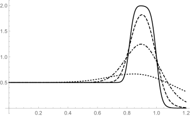
$r/r_{n}$

Figure 1: The normalized radial density of states for the Majorana zero modes of a giant vortex with the winding number $n=4$ (dotted line), $n=16$ (dashed-dotted line), $n=64$ (dashed line), and $n=256$ (solid line).

So far we have considered the case $\kappa={\cal O}(1)$. For $\kappa\gg 1$ there appears another condition on the allowed values of $n$. The method [15, 16] relies on the scale hierarchy $\delta/r_{n}\ll 1$. This scale ratio is proportional to $\sqrt{\kappa/n}$. For $\kappa>n$ the magnetic field is expelled from the vortex core and the vortex cannot be considered as a thin-wall flux tube. At the same time, the superconductors with the large value of the Ginzburg-Landau parameter may not be ideal for the experimental realization of the giant vortices. Indeed, the free energy in this case grows with $n$ as $n^{2}\ln\kappa$ while for $\kappa={\cal O}(1)$ it scales as $n/\kappa$ [16]. This makes the giant vortices for large $\kappa$ much less stable against the decay into the elementary vortices and, hence, more difficult to create in an experiment.

In any case, an experimental realization of the giant Abrikosov vortices with $n={\cal O}(10)$ may not be an easy task. At the same time the hard wall giant vortices of arguably very large $n$ can be created by a magnetic flux flowing through a hole in the superconducting film on the surface of the topological insulator. Such a design has been originally suggested in Ref. [8] for a physical realization of the Sachdev-Ye-Kitaev model on the hole boundary, but it can also be an ideal place for the study of two-dimensional Majorana zero modes in the hole interior. The result Eq. (12) in this case should be adjusted. The term $f^{\prime}/f$ in Eq. (6) now gets a very large positive constant contribution proportional to the ratio of the Cooper pair chemical potential to the superconductor energy gap. This effectively makes the Andreev reflection short-range so that all the states with $l\;\hbox to0.0pt{\lower 3.5pt\hbox{$\mathchar 0\relax\sim$}\hss}\raise 1.0pt\hbox{$>$}\;n/2$ get localized on the hole edge. The radial density of states now takes the form

$$\rho(r)\sim{\rho_{0}\over 2}\left(1+{R\over 2}\delta(r-R)\right)\,,$$ (13)

where $\rho_{0}={2n/R^{2}}$ and $R$ is the hole radius. The delta-function in the above equation is in fact an approximation of the non-Gaussian peak with the width of order $\delta\ll R$, and $R$ should be taken larger than $r_{n}$ for a given $n$ and $\zeta$ to have a stable vortex configuration.

Though the spatial distributions in Eq. (12) and Eq. (13) are quite similar, the physical properties of the two systems are qualitatively different. For Abrikosov vortices the parameter $\rho_{0}$ which defines the average density of states is $n$-independent and completely determined by the intrinsic properties of the superconductor through the geometric average $\zeta$ of the magnetic penetration and the correlation length. By contrast, for the hard-wall vortices the parameter $\rho_{0}$ is quantized in the units of ${2/R^{2}}$ and is proportional to the number of the magnetic flux quanta. Thus, it can be discreetly changed by the variation of the applied magnetic field $B$. The corresponding average rate of the density variation inside the core evaluates to

$${d\rho\over dB}=\pi K_{J}\,,$$ (14)

where $K_{J}$ is the Josephson constant (the inverse of the magnetic flux quantum).

Our solution Eq. (10) is qualitatively different from the existing analysis where the role of the magnetic field on the formation of the vortex states has been neglected. This is indeed justified for an elementary vortex and for the large values of the Ginzburg-Landau parameter $\kappa\gg 1$ when the vortex states are predominantly formed through the Andreev reflection and are localized near the core boundary [21, 22, 23]. However, with the increasing winding number the magnetic flux through the vortex core grows and for the giant vortices with $n\gg\kappa$ the zero modes are formed through a fine interplay between the magnetic effects and the long-range Andreev reflection resulting in a set of the warped lowest Landau level states. Note that the effect of the magnetic field on the delocalization of the zero modes for the elementary vortex lattice has been recently discussed in Ref. [24].

To conclude, we have applied an advanced asymptotic method based on the scale separation and the expansion in inverse powers of the winding number to find the analytical solution for the Majorana zero modes of the giant vortices. In the case of the Abrikosov vortices the solution reveals a nontrivial dynamical origin and a simple universal structure, provided the vortex winding number exceeds the value of the Ginzburg-Landau parameter of the superconductor. It is not sensitive to the form of the pair potential and is completely determined by a single parameter, the vortex radius, which can be directly measured in the experiment. The resulting local density of states is confined to the vortex core, where the non-zero modes are magnetically gapped. The density has a characteristic profile which can be used as a signature for the identification of the Majorana zero modes by scanning electron microscopy [12]. For the hard-wall giant vortices in the specially designed heterostructures [8] we have found that a half of the zero modes are pinned to the vortex edge with the other half filling the vortex core. The dependence of the energy on the applied magnetic field, characteristic of the non-zero modes, can therefore be used for a clear identification of the Majorana core states. Moreover, the density of the zero modes is quantized and changes discreetly under the variation of the magnetic field with the universal average rate given by the Josephson constant. These features establish the giant vortices as an ideal laboratory for the search of compelling experimental evidence of the Majorana fermions in two dimensions.

Acknowledgments. We would like to thank Joseph Maciejko for many useful discussions. The work of L.G. was supported through by NSERC. The work of A.P. was supported in part by NSERC and the Perimeter Institute for Theoretical Physics.

References

- [1] J. Alicea, Rep. Prog. Phys. 75, 076501 (2012).
- [2] C. W. J. Beenakker, Annu. Rev. Condens. Matter Phys. 4, 113 (2013).
- [3] S. R. Elliott and M. Franz, Rev. Mod. Phys. 87, 137 (2015).
- [4] G. E. Volovik, JETP Lett. 70, 609-614 (1999).
- [5] N. Read and D. Green, Phys. Rev. B 61, 10267 (2000).
- [6] L. Fu and C. L. Kane, Phys. Rev. Lett. 100, 096407 (2008).
- [7] R. Jackiw and P. Rossi, Nucl. Phys. B 190, 681 (1981).
- [8] D. I. Pikulin and M. Franz, Phys. Rev. X 7, 031006 (2017).
- [9] T. Cren, L. Serrier-Garcia, F. Debontridder, and D. Roditchev, Phys. Rev. Lett. 107, 097202 (2011).
- [10] H. H. Sun et al., Phys. Rev. Lett. 116, 257003 (2016).
- [11] D. Wang et al., Science 362, 333 (2018).
- [12] T. Zhang et al., Phys. Rev. Lett. 126, 127001 (2021).
- [13] E. J. Weinberg, Phys. Rev. D 24, 2669 (1981).
- [14] S. Tewari, S. Das Sarma, and D.-H. Lee, Phys. Rev. Lett. 99, 037001 (2007).
- [15] A. A. Penin and Q. Weller, Phys. Rev. Lett. 125, 251601 (2020).
- [16] A. A. Penin and Q. Weller, JHEP 08, 056 (2021).
- [17] A. A. Abrikosov, Sov. Phys. JETP 5, 1174 (1957) [Zh. Eksp. Teor. Fiz. 32, 1442 (1957)].
- [18] C. Chamon, R. Jackiw, Y. Nishida, S. Y. Pi, and L. Santos, Phys. Rev. B 81, 224515 (2010).
- [19] J. D. Shore, M. Huang, A. T. Dorsey, and J. P. Sethna, Phys. Rev. Lett. 62, 3089 (1989).
- [20] S. Bolognesi, Nucl. Phys. B 730, 127 (2005).
- [21] C. Caroli, P. G. De Gennes, and J. Matricon, Phys. Lett. 9, 307 (1964).
- [22] J. Bardeen, R. Kümmel, A. E. Jacobs, and L. Tewordt, Phys. Rev. 187, 556 (1969).
- [23] S. M. M. Virtanen and M. M. Salomaa, Phys. Rev. B 60, 14581 (1999).
- [24] M. J. Pacholski, G. Lemut, O. Ovdat, İ. Adagideli, and C. W. J. Beenakker, Phys. Rev. Lett. 126, 226801 (2021).