Robust Adaptive Neural Network Control of Time-Varying State Constrained Nonlinear Systems

Abstract

This paper deals with the tracking control problem for a very simple class of unknown nonlinear systems. In this paper, we presents a design strategy for tracking control of time-varying state constrained nonlinear systems in an adaptive framework. The controller is designed using the backstepping method. While designing it, Barrier Lyapunov Function (BLF) is used so that the state variables do not contravene its constraints. In order to cope with the unknown dynamics of the system, an online approximator is designed using a neural network with a novel adaptive law for its weight update. To make the controller robust and computationally inexpensive, a disturbance observer is proposed to cope with the disturbance along with neural network approximation error and the time derivative of virtual control input. The effectiveness of the proposed approach is demonstrated through a simulation study.

I Introduction

Recently, researchers in the field of nonlinear control systems have made significant efforts to address the issue of system state and output stability. However, in everyday life, numerous uncertain dynamic systems have constraints such as performance, saturation, physical stoppages, and safety specifications. Constraints are ineludible for such systems when designing controllers in real-time. In practical systems, constraints can be static or dynamic, and their upper and lower bounds can be symmetric or asymmetric. The Barrier Lyapunov Function (BLF) has been widely used in the literature to deal with such systems. In order to design a controller for a system with static symmetric or asymmetric constraints, [1] provides a nice integration of BLF with the well-known backstepping technique. Other than the BLF-based technique, other efforts have been undertaken by academia and industry to design a controller for the constrained system, including error transformation and model predictive control (MPC). In error transformation, the application of tangent hyperbolic in a prescribed function may lead to a singularity problem, and exorbitant control input may violate prescribed control performance, leading to instability. In MPC, linear and nonlinear system constraints are addressed by solving a finite horizon open-loop optimal control problem [2]. Most optimal control and MPC rely on numerical, computationally intensive algorithms to solve control problems [3]. BLF has been studied for the controller design of constrained systems because it easily handles unknown system dynamics, uncertainties, and disturbances by integrating robust adaptive backstepping or sliding mode control. In [4, 5, 6, 7, 8, 9], authors have used BLF to design controller for static state constrained nonlinear systems. Further, in [10, 11, 12, 13, 14, 15, 16], authors have designed controller for time-varying state constrained nonlinear systems, however design are not robust.

Motivated by the aforementioned works, the contributions of this paper are listed below.

1. A novel adaptive law for neural networks (NN) is designed to deal with unknown dynamics of the systems.

2. To deal with the uncertainties such as disturbance, approximation error and explosion of derivative of virtual control law in the backstepping design, a novel disturbance observer has been proposed.

3. Further, to deal with unknown control gain a novel controller has been proposed using Nussbaum gain.

The paper is organized as follows. In Section II, we present the system description and problem statement. This section also presents some assumptions, definition, and lemmas for the stability analysis of the system. Section III discusses the construction of NN for the approximation of unknown terms involved in the design; Section IV consists of two subsections. Subsection IV-A discusses the design of a disturbance observer for the robustness of the system, and Subsection IV-B discusses the steps to design an adaptive controller using the backstepping technique. Section V discusses the theorem for the boundedness of the signals in the closed-loop system. Section VI illustrates the proposed methodology using the simulation examples. Finally, Section VII concludes the paper.

II System Description and Problem Statement

Consider a class of SISO nonlinear systems shown below

$$\begin{split}\dot{x}_{i}&=x_{i+1}+d_{i}\left(t\right)~{}~{}~{}~{}\forall i\in\{1,\ldots,n-1\}\\ \dot{x}_{n}&=f\left(x\right)+\beta u+d_{n}\left(t\right)\\ y&=x_{1}\end{split}$$ (1)

where $x_{i}\in\mathbb{R}$, $\forall i\in\mathbb{N}_{n}$, $u\in\mathbb{R}$ and $y\in\mathbb{R}$ are the $i^{th}$ state, the control input, and the output of the system, respectively; $f\left(x\right)$ $\in\mathbb{R}$ is smooth unknown nonlinear functions and $\beta$ is unknown control coefficient; $d_{i}\in\mathbb{R},\forall i\in\mathbb{N}_{n}$ are unknown time-varying bounded disturbance. In this study, states are considered to be constrained such that, $\mathinner{\!\left\lvert x_{i}\right\rvert}<\Psi_{i}(t)$, where $\Psi_{i}\in\mathbb{R}$ is a known time varying state constraint on the state variable.

Problem Statement: The goal of this paper is to design a NN-based adaptive controller for (1) such that (i) output $y$ tracks the desired output $y_{d}$; (ii) all the closed-loop signals are guaranteed to be bounded; and (iii) all the system states do not contravene their state constraints.

Following are the assumptions, definition and lemmas, which will be needed to achieve the control objective.

Assumption 1 [17]: The control coefficient $\beta\neq 0$.

Assumption 2 [18]: The unknown time-varying disturbance $d_{i}(t)$ is bounded and there exist some positive constant $d_{0}$ such that $\mathinner{\!\left\lvert\dot{d}_{i}(t)\right\rvert}\leq d_{0}$ $\forall i\in\mathbb{N}_{n}$.

Assumption 3 [19, 17, 20]. The first $n$th time derivative of desired output $y_{d}$ is bounded $\forall t\in[0,\infty)$.

Remark 1: For the computation of time derivative of virtual control input, we need time derivative of desired output in each step of backstepping based scheme, so its availability and boundedness is a must. However, here we have relaxed the availability by estimating the time derivative of virtual control input using the disturbance observer.

Assumption 4 [21]. The time-varying symmetric state constraint $\Psi_{i}(t)\in\mathbb{R}$ is bounded $\forall t\in[0,\infty)$.

Definition 1 [22] : The function $\mathcal{N}(\zeta)$ is said to be Nussbaum, if it holds the following property:

$$\begin{split}\underset{s\rightarrow\infty}{\lim}\sup\frac{1}{s}\int_{0}^{s}\mathcal{N}(\zeta)d\zeta=+\infty\\ \underset{s\rightarrow\infty}{\lim}\inf\frac{1}{s}\int_{0}^{s}\mathcal{N}(\zeta)d\zeta=-\infty.\end{split}$$ (2)

There are several functions that can be considered Nussbaum functions, including $e^{\zeta^{2}}\cos((\pi/2)\zeta)$ and $\zeta^{2}cos(\zeta)$. In this paper, we have used $\mathcal{N}(\zeta)=\zeta^{2}cos(\zeta)$ as a Nussbaum function.

Lemma 1 [18]: Let $\mathcal{V}(t)\geq 0$ and $\zeta(t)$ be smooth functions defined on $[0,t_{f})$ and $\mathcal{N}(\zeta(t))$ be an even smooth Nussbaum function. If the following inequality holds:

$$\mathcal{V}(t)\leq\kappa_{1}+e^{-\kappa_{2}t}\int_{0}^{t}\left({\beta_{0}\mathcal{N}(\zeta)}+1\right)\dot{\zeta}e^{\kappa_{2}\tau}d\tau$$ (3)

where $\kappa_{1}$ and $\kappa_{2}$ are positive constant, and $\beta_{0}$ is a non-zero constant, then $\mathcal{V}(t)$, $\zeta(t)$ and $\int_{0}^{t}{\beta_{0}\mathcal{N}(\zeta)}\dot{\zeta}d\tau$ are bounded on $[0,t_{f})$.

Lemma 2 [23]: For any $z$ in the interval $\mathinner{\!\left\lvert z\right\rvert}<\mathinner{\!\left\lvert\psi\right\rvert}$, where $\psi\in\mathbb{R}$, we have

$$\log\frac{\psi^{2}}{\psi^{2}-z^{2}}<\frac{z^{2}}{\psi^{2}-z^{2}}.$$ (4)

III NN Approximation

The function $f(x)$ is not known in the system (1). This section will look at an online approximation strategy for dealing with an unknown function. For this, Radial Basis Function (RBF) NN is used. It is well known that using the universal approximation property of RBF NN, we can approximate any unknown continuous function. The RBF NN used here has $l$ number of hidden neurons and a output. The output of the network $O_{NN}(\theta,\bar{z})\in\mathbb{R}$ is given by

$$O_{NN}(\theta,\bar{z})=\theta^{T}\varphi(\bar{z})\quad$$ (5)

where the vector $\bar{z}=[x_{1},\ldots,x_{n}]^{T}$ is the input of the NN, $\theta=[\theta_{i},\ldots,\theta_{l}]\in\mathbb{R}^{l}$ is the weight vector, $\varphi(\bar{z})\in\mathbb{R}^{l}$ is a basis vector of RBF NN with a set of suitably chosen Gaussian basis function $(\varphi_{i}\in\mathbb{R}$, $\forall i\in\mathbb{N}_{l})$ defined on a compact set $\Omega_{\bar{z}}$, such that $\varphi=[\varphi_{1}(\bar{z}),\ldots,\varphi_{l}(\bar{z})]^{T}$ and

$$\varphi_{i}(\bar{z})=exp\left(\frac{-\mathinner{\!\left\lVert\bar{z}-c_{i}\right\rVert}^{2}}{b_{i}}\right)\qquad\forall i\in\mathbb{N}_{l}$$ (6)

where $c_{i}\in\Omega_{\bar{z}}$ is the centre of receptive field and $b_{i}\in\mathbb{R}$ is the width of Gaussian function. From the definition of $\varphi_{i}(\bar{z})$, we find that it is bounded. Let say $\bar{\varphi}$ be the upper bound of $\varphi_{i}(\bar{z})$ then

$$\mathinner{\!\left\lVert\varphi(\bar{z})\right\rVert}\leq\bar{\varphi}.$$ (7)

Assuming that an ideal weight vector $\theta^{*}=[\theta^{*}_{1},\ldots,\theta^{*}_{l}]\in\mathbb{R}^{l}$ exists, such that

$$f(x)=\theta^{*T}\varphi(\bar{z})+\epsilon(\bar{z})\quad$$ (8)

where, $\theta^{*}$ and $\epsilon$ are ideal weight vector and approximation error respectively.

Assumption 5. The approximation error vector $\epsilon$ is bounded and $\mathinner{\!\left\lvert\epsilon\right\rvert}\leq\bar{\epsilon}$ for some positive constant $\bar{\epsilon}$.

The ideal weight vector $\theta^{*}$ is defined as follows

$$\begin{split}\theta^{*}=\arg\underset{\theta^{*}\in\mathbb{R}^{l}}{\min}\left\{{\sup}\left(O_{NN}(\theta^{*},\bar{z})-O_{NN}(\theta,\bar{z})\right)\right\}.\end{split}$$ (9)

Using (8), the system (1) can be rewritten as

$$\dot{x}_{i} =x_{i+1}+d_{i}\left(t\right)~{}~{}~{}~{}~{}\forall i\in\mathbb{N}_{n-1}$$ (10)

$$\dot{x}_{n} =\theta^{*T}\varphi(\bar{z})+\epsilon(\bar{z})+\beta u+d_{n}\left(t\right).$$ (11)

The ideal weight matrix $\theta^{*}$ above is not known and therefore needs to be estimated. Let $\hat{\theta}=[\hat{\theta}_{1},\ldots,\hat{\theta}_{l}]\in\mathbb{R}^{l}$ be the estimate of ideal weight matrix $\theta^{*}$ such that

$$\hat{f}(x)=\hat{\theta}^{T}\varphi(\bar{z})$$ (12)

where $\hat{f}(x)$ is an approximation of the unknown nonlinear function $f(x)$. The next steps of controller design have been presented in the following section.

IV Robust Adaptive Backstepping Controller Design

Let $z=[z_{1},\ldots,z_{n}]^{T}$, $v=[v_{1},\ldots,v_{n-1}]^{T}$, and $v_{0}=x_{1d}$ be an error vector, virtual control input vector, and desired output vector respectively. The error vector elements are defined as follows

$$\begin{split}z_{i}&=x_{i}-v_{i-1}\qquad\forall i\in\mathbb{N}_{n}.\\ \end{split}$$ (13)

Note: To maintain the uniformity in the expression for the error variables, it is common practice to denote the desired output with a symbol, similar to virtual control input with $0$ in subscript.

On differentiating (13) with respect to time and using (10), $\forall i\in\mathbb{N}_{n-1}$ the error dynamics is

$$\dot{z}_{i} =x_{i+1}+d_{i}(t)-\dot{v}_{i-1},$$ (14)

and taking the time derivative of (13) and using (11) for $i=n$, we have error dynamics

$$\dot{z}_{n} =\theta^{*T}\varphi(\bar{z})+\epsilon(\bar{z})+\beta u+d_{n}\left(t\right)-\dot{v}_{n-1}.$$ (15)

IV-A Disturbance Observer

The calculation of the derivative of virtual control input is a major computing step in backstepping-based controller design. The derivative of this control input must be estimated. The disturbance observer is designed to have an estimate including the unknown disturbance.

The observer variable $\varepsilon=[\varepsilon_{1},\ldots,\varepsilon_{n}]^{T}\in\mathbb{R}^{n}$ is defined as

$$\varepsilon_{i} =d_{i}(t)-\dot{v}_{i-1},\text{ }\forall i\in\mathbb{N}_{n-1}$$ (16)

$$\varepsilon_{n} =\epsilon(\bar{z})+(\beta-1)u+d_{n}\left(t\right)-\dot{v}_{n-1}.$$ (17)

Assumption 6. The observer variable $\varepsilon_{i}$, to be estimated, is bounded and $\forall i\in\mathbb{N}_{n}$ there exists a positive constant $\rho_{i}$ such that its derivative $\mathinner{\!\left\lvert\dot{\varepsilon}_{i}\right\rvert}\leq\bar{\varepsilon}_{i}$.

The error dynamics (14) and (15) can be expressed using (16) and (17) respectively as

$$\dot{z}_{i} =x_{i+1}+\varepsilon_{i},\text{ }\forall i\in\mathbb{N}_{n-1}$$ (18)

$$\dot{z}_{n} =\theta^{*T}\varphi(\bar{z})+u+\varepsilon_{n}.$$ (19)

To estimate the observer variable in (16) and (17) an auxiliary system is introduced. It is defined as

$$\eth_{i} =\varepsilon_{i}-k_{\varepsilon_{i}}z_{i},\quad\forall i\in\mathbb{N}_{n}$$ (20)

where $k_{\varepsilon_{i}}$ is an observer gain.

Using (18) and (19), we can rewrite the dynamics of auxiliary system (20) as

$$\dot{\eth}_{i} =\dot{\varepsilon}_{i}-k_{\varepsilon_{i}}(x_{i+1}+\varepsilon_{i}),\quad\forall i\in\mathbb{N}_{n-1}$$ (21)

$$\dot{\eth}_{n} =\dot{\varepsilon}_{n}-k_{\varepsilon_{n}}(\theta^{*T}\varphi(\bar{z})+u+\varepsilon_{n}).$$ (22)

To estimate the auxiliary system, the observer dynamics is proposed as

$$\dot{\hat{\eth}}_{i} =-k_{\varepsilon_{i}}(x_{i+1}+\hat{\varepsilon}_{i})~{}~{}\text{and}$$ (23)

$$\dot{\hat{\eth}}_{n} =-k_{\varepsilon_{n}}(\hat{\theta}^{T}\varphi(\bar{z})+u+\hat{\varepsilon}_{n}).$$ (24)

Using (20), the estimate of observer variables (16) and (17) can be obtained as

$$\hat{\varepsilon}_{i}=\hat{\eth}_{i}+k_{\varepsilon_{i}}z_{i},\quad\forall i\in\mathbb{N}_{n}.$$ (25)

Using (20) and (25), the estimation error $\tilde{\eth}_{i}$ of the auxiliary system can be written as

$$\tilde{\eth}_{i}=\eth_{i}-\hat{\eth}_{i}=\tilde{\varepsilon}_{i},\quad\forall i\in\mathbb{N}_{n}.$$ (26)

Subtracting (23) and (24) from (21) and (22) respectively, and using (26), the observer error dynamics for the auxiliary system becomes

$$\dot{\tilde{\eth}}_{i} =\dot{\tilde{\varepsilon}}_{i}=\dot{\varepsilon}_{i}-k_{\varepsilon_{i}}\tilde{\varepsilon}_{i},\quad\forall i\in\mathbb{N}_{n-1}$$ (27)

$$\dot{\tilde{\eth}}_{n} =\dot{\tilde{\varepsilon}}_{n}=\dot{\varepsilon}_{n}-k_{\varepsilon_{n}}(-\tilde{\theta}^{T}\varphi(\bar{z})+\tilde{\varepsilon}_{n}),$$ (28)

where $\tilde{\theta}=\hat{\theta}-\theta^{*}$ and $\tilde{\varepsilon}_{i}=\varepsilon_{i}-\hat{\varepsilon},$ $\forall i\in\mathbb{N}_{n}$.

IV-B Controller Design and Stability Analysis

To begin, first we will define $n$ BLF for the $n$ states of the system (1) as well as their time derivative will be calculated.

Let $\mathcal{L}_{i}$, $i=1,\ldots,n$ be a BLF and defined as

$$\mathcal{L}_{i}=\frac{1}{2}\log\frac{\psi_{i}^{2}(t)}{\psi_{i}^{2}(t)-z_{i}^{2}},$$ (29)

where $\psi_{i}(t)$ is a constraint on error variable $z_{i}$, which will be defined later. Taking the time derivative of (29), we have

$$\dot{\mathcal{L}}_{i}={\mathcal{Q}}_{i}\left(\dot{z}_{i}-\frac{z_{i}}{\psi_{i}}\dot{\psi}_{i}\right),$$ (30)

$$\text{where~{}}{\mathcal{Q}}_{i}=\frac{z_{i}}{\psi_{i}^{2}-z_{i}^{2}}.$$ (31)

Following (14) and substituting $z_{i}=x_{i}-v_{i-1}$ in (30), we have

$$\dot{\mathcal{L}}_{i}={\mathcal{Q}}_{i}\left(\dot{x}_{i}-\dot{v}_{i-1}-\frac{z_{i}}{\psi_{i}}\dot{\psi}_{i}\right).$$ (32)

The design steps of controller are as follows:

Step 1: Consider a Lyapunov function $\mathcal{V}_{1}$, as

$${\mathcal{V}}_{1}=\mathcal{L}_{1}+\frac{1}{2}\tilde{\varepsilon}^{2}_{1}.$$ (33)

Taking the time derivative of (33) and using (30), we have

$$\dot{\mathcal{V}}_{1}={\mathcal{Q}}_{1}\left(\dot{z}_{1}-\frac{z_{1}}{\psi_{1}}\dot{\psi}_{1}\right)+{\tilde{\varepsilon}}_{1}\dot{\tilde{\varepsilon}}_{1}.$$ (34)

On substituting (18) for $i=1$ in (34), we have

$$\dot{\mathcal{V}}_{1}={\mathcal{Q}}_{1}\left(x_{2}+\varepsilon_{1}-\frac{z_{1}}{\psi_{1}}\dot{\psi}_{1}\right)+{\tilde{\varepsilon}}_{1}\dot{\tilde{\varepsilon}}_{1}.$$ (35)

On substituting (27) for $i=1$ in (35), we have

$$\dot{\mathcal{V}}_{1}={\mathcal{Q}}_{1}x_{2}+{\mathcal{Q}}_{1}\varepsilon_{1}-{\mathcal{Q}}_{1}\frac{z_{1}}{\psi_{1}}\dot{\psi}_{1}+{\tilde{\varepsilon}}_{1}\dot{\varepsilon}_{1}-k_{\varepsilon_{1}}\tilde{\varepsilon}_{1}^{2}.$$ (36)

Following (13), and substituting $x_{2}=z_{2}+v_{1}$ in (36) leads to

$$\dot{\mathcal{V}}_{1}={\mathcal{Q}}_{1}z_{2}+{\mathcal{Q}}_{1}v_{1}+{\mathcal{Q}}_{1}\varepsilon_{1}-{\mathcal{Q}}_{1}\frac{z_{1}}{\psi_{1}}\dot{\psi}_{1}+{\tilde{\varepsilon}}_{1}\dot{\varepsilon}_{1}-k_{\varepsilon_{1}}\tilde{\varepsilon}_{1}^{2}.$$ (37)

Choose the virtual controller $v_{1}$ as

$$v_{1} =\mathcal{N}_{1}(\zeta_{1})\alpha_{1},~{}\text{where}$$ (38)

$$\dot{\zeta}_{1} =\mathcal{Q}_{1}\alpha_{1},~{}\text{and}$$ (39)

$$\alpha_{1} =k_{1}z_{1}+\hat{\varepsilon}_{1}+{\mathcal{Q}_{1}}-\frac{z_{1}}{\psi_{1}}{\dot{\psi}_{1}},$$ (40)

and the design parameter $k_{1}>0$.

Using (38)-(40), (37) becomes

$$\dot{\mathcal{V}}_{1} =-k_{1}\mathcal{Q}_{1}z_{1}+\mathcal{Q}_{1}z_{2}+\mathcal{N}_{1}(\zeta_{1})\dot{\zeta}_{1}+\dot{\zeta}_{1}$$

$$\quad+\mathcal{Q}_{1}{\tilde{\varepsilon}_{1}}+{\tilde{\varepsilon}}_{1}\dot{\varepsilon}_{1}-k_{\varepsilon_{1}}\tilde{\varepsilon}_{1}^{2}-{\mathcal{Q}_{1}^{2}}.$$ (41)

For further analysis, we need few inequality relations. They are as follows

1. First term of (IV-B), i.e., $k_{1}\mathcal{Q}_{1}z_{1}$:
   Following (31) and using Lemma 2, we have

   $$-\frac{1}{2}\mathcal{Q}_{1}z_{1}=-\frac{1}{2}\frac{z_{1}^{2}}{\psi_{1}^{2}-z_{1}^{2}}\leq-\frac{1}{2}\log\frac{\psi_{1}^{2}}{\psi_{1}^{2}-z_{1}^{2}}.$$ (42)

   Multiplying (42) on both sides by $2k_{1}$, we have

   $$-k_{1}\mathcal{Q}_{1}z_{1}\leq-2k_{1}\mathcal{L}_{1}.$$ (43)

1. Second term of (IV-B), i.e., $\mathcal{Q}_{1}z_{2}$ :
   Using the Young’s inequality, we have

   $$\mathcal{Q}_{1}z_{2}\leq\frac{\mathcal{Q}_{1}^{2}}{2}+\frac{z_{2}^{2}}{2}$$ (44)

1. Fifth, sixth, and seventh term of (IV-B), i.e., $\mathcal{Q}_{1}{\tilde{\varepsilon}_{1}}+{\tilde{\varepsilon}}_{1}\dot{\varepsilon}_{1}-k_{\varepsilon_{1}}\tilde{\varepsilon}_{1}^{2}$.

Following Assumption 6, and using Young’s inequality, we have

$$\mathcal{Q}_{1}{\tilde{\varepsilon}_{1}}+{\tilde{\varepsilon}}_{1}\dot{\varepsilon}_{1}-k_{\varepsilon_{1}}\tilde{\varepsilon}_{1}^{2} \leq\frac{\tilde{\varepsilon}_{1}^{2}}{2}+\frac{\mathcal{Q}_{1}^{2}}{2}+\frac{\tilde{\varepsilon}_{1}^{2}}{2}+\frac{{\bar{\varepsilon}}_{1}^{2}}{2}-k_{\varepsilon_{1}}{\tilde{\varepsilon}}^{2}_{1},$$

$$=-\tilde{\varepsilon}_{1}^{2}\left(k_{\varepsilon_{1}}-1\right)+\frac{\mathcal{Q}_{1}^{2}}{2}+\frac{{\bar{\varepsilon}}_{1}^{2}}{2}.$$ (45)

Using the inequalities (43) and (IV-B), in (IV-B), we have

$$\dot{\mathcal{V}}_{1} \leq \mathcal{N}_{1}(\zeta_{1})\dot{\zeta}_{1}+\dot{\zeta}_{1}-2k_{1}{\mathcal{L}}_{1}+z_{2}^{2}$$ (46)

$$-\tilde{\varepsilon}_{1}^{2}\left(k_{\varepsilon_{1}}-1\right)+\varrho_{1}.$$

where $\varrho_{1}=\frac{{\bar{\varepsilon}}_{1}^{2}}{2}$.

Equation (46) can be further written as

$$\dot{\mathcal{V}}_{1} \leq-\mu_{1}\mathcal{V}_{1}+\mathcal{N}_{1}(\zeta_{1})\dot{\zeta}_{1}+\dot{\zeta}_{1}+z_{2}^{2}+\varrho_{1},$$ (47)

where $\mu_{1}=\min\left(2k_{1},2\left(k_{\varepsilon_{1}}-1\right)\right)$.

In the decoupled backstepping design, we will seek for the boundedness of $z_{2}$ in the next step of the design rather than cancellation of $z_{2}^{2}$.

Multiplying both sides of (47) by $e^{\mu_{1}t}$, we have

$$\frac{d(\mathcal{V}_{1}(t)e^{\mu_{1}t})}{dt}\leq\left({\mathcal{N}}_{1}(\zeta_{1})\dot{\zeta}_{1}+\dot{\zeta}_{1}+z_{2}^{2}+\varrho_{1}\right)e^{\mu_{1}t}.$$ (48)

Integrating (48) over $\left[0,t\right]$, gives

$$e^{\mu_{1}t}\mathcal{V}_{1}(t) \leq\mathcal{V}_{1}(0)+\int_{0}^{t}{\left({\mathcal{N}}_{1}(\zeta_{1})+1\right)\dot{\zeta}_{1}e^{\mu_{1}\tau}d\tau}$$

$$\quad+\int_{0}^{t}{z_{2}^{2}e^{\mu_{1}\tau}d\tau}+\frac{\varrho_{1}e^{\mu_{1}t}}{\mu_{1}}-\frac{\varrho_{1}}{\mu_{1}}.$$ (49)

On multiplying both sides of (49) by $e^{-\mu_{1}t}$, we have

$$\mathcal{V}_{1}(t) \leq e^{-\mu_{1}t}\mathcal{V}_{1}(0)+e^{-\mu_{1}t}\int_{0}^{t}{\left({\mathcal{N}}_{1}(\zeta_{1})+1\right)\dot{\zeta}_{1}e^{\mu_{1}\tau}d\tau}$$

$$\quad+e^{-\mu_{1}t}\int_{0}^{t}{z_{2}^{2}e^{\mu_{1}\tau}d\tau}+\frac{\varrho_{1}}{\mu_{1}}-\frac{\varrho_{1}e^{-\mu_{1}t}}{\mu_{1}}.$$ (50)

Since, $0<e^{-\mu_{1}t}\leq 1$, we can write (50) as

$$\mathcal{V}_{1}(t) \leq\mathcal{V}_{1}(0)+e^{-\mu_{1}t}\int_{0}^{t}{\left({\mathcal{N}}_{1}(\zeta_{1})+1\right)\dot{\zeta}_{1}e^{\mu_{1}\tau}d\tau}$$

$$\quad+e^{-\mu_{1}t}\int_{0}^{t}{z_{2}^{2}e^{\mu_{1}\tau}d\tau}+\frac{\varrho_{1}}{\mu_{1}}-\frac{\varrho_{1}e^{-\mu_{1}t}}{\mu_{1}}.$$ (51)

We can rewrite (51) as

$$\mathcal{V}_{1}(t) \leq\mathcal{V}_{1}(0)+e^{-\mu_{1}t}\int_{0}^{t}{\left({\mathcal{N}}_{1}(\zeta_{1})+1\right)\dot{\zeta}_{1}e^{\mu_{1}\tau}d\tau}$$

$$\quad+e^{-\mu_{1}t}\int_{0}^{t}{z_{2}^{2}e^{\mu_{1}\tau}d\tau}+\frac{\varrho_{1}}{\mu_{1}}.$$ (52)

In (51), if there would have been no extra term, i.e. $e^{-\mu_{1}t}\int_{0}^{t}{z_{2}^{2}e^{\mu_{1}\tau}d\tau}$, then using Lemma 1, we may have shown that $\mathcal{V}_{1}(t),\zeta_{1}$ and $z_{1},\hat{\varepsilon}_{1}$ are all uniformly ultimately bounded. However, if we can show $z_{2}$ is bounded, then using the following relation

$$e^{-\mu_{1}t}\int_{0}^{t}{z_{2}^{2}e^{\mu_{1}\tau}d\tau} \leq e^{-\mu_{1}t}\underset{\tau\in[0,t]}{\sup}z_{2}^{2}\int_{0}^{t}{e^{\mu_{1}\tau}d\tau}$$

$$\leq\frac{\underset{\tau\in[0,t]}{\sup}z_{2}^{2}}{\mu_{1}},$$ (53)

we can say that $e^{-\mu_{1}t}\int_{0}^{t}{z_{2}^{2}e^{\mu_{1}\tau}d\tau}$ is bounded. Consequently using Lemma 1, we will be able to show $\mathcal{V}_{1}(t),\zeta_{1}$ and $z_{1},\hat{\varepsilon}_{1}$ are also bounded. Again to show $z_{2}$ is bounded, we need to follow similar steps. The process will be recursive until we do not have $z_{i+1}^{2}$ in the derivative of Lyapunov function.

Step i $(i=2,\ldots,n-1)$: Consider a Lyapunov function

$${\mathcal{V}}_{i}=\mathcal{L}_{i}+\frac{1}{2}\tilde{\varepsilon}^{2}_{i}.$$ (54)

Taking the time derivative of (54) and using (30), (54) becomes

$$\dot{\mathcal{V}}_{i}={\mathcal{Q}}_{i}\left(\dot{z}_{i}-\frac{z_{i}}{\psi_{i}}\dot{\psi}_{i}\right)+{\tilde{\varepsilon}}_{i}\dot{\tilde{\varepsilon}}_{i}.$$ (55)

On substituting (18) in (55), we have

$$\dot{\mathcal{V}}_{i}={\mathcal{Q}}_{i}\left(x_{i+1}+\varepsilon_{i}-\frac{z_{i}}{\psi_{i}}\dot{\psi}_{i}\right)+{\tilde{\varepsilon}}_{i}\dot{\tilde{\varepsilon}}_{i}.$$ (56)

On substituting (27) in (56), we have

$$\dot{\mathcal{V}}_{i}={\mathcal{Q}}_{i}x_{i+1}+{\mathcal{Q}}_{i}\varepsilon_{i}-{\mathcal{Q}}_{i}\frac{z_{i}}{\psi_{i}}\dot{\psi}_{i}+{\tilde{\varepsilon}}_{i}\dot{\varepsilon}_{i}-k_{\varepsilon_{i}}\tilde{\varepsilon}_{i}^{2}.$$ (57)

Following (13), and substituting $x_{i}=z_{i}+v_{i-1}$ in (57) leads to

$$\dot{\mathcal{V}}_{i}={\mathcal{Q}}_{i}z_{i+1}+{\mathcal{Q}}_{i}v_{i}+{\mathcal{Q}}_{i}\varepsilon_{i}-{\mathcal{Q}}_{i}\frac{z_{i}}{\psi_{i}}\dot{\psi}_{i}+{\tilde{\varepsilon}}_{i}\dot{\varepsilon}_{i}-k_{\varepsilon_{i}}\tilde{\varepsilon}_{i}^{2}.$$ (58)

Choose the virtual controller $v_{i}$ as

$$v_{i} =\mathcal{N}_{i}(\zeta_{i})\alpha_{i},~{}\text{where}$$ (59)

$$\dot{\zeta}_{i} =\mathcal{Q}_{i}\alpha_{i},~{}\text{and}$$ (60)

$$\alpha_{i} =k_{i}z_{i}+\hat{\varepsilon}_{i}+\mathcal{Q}_{i}-\frac{z_{i}}{\psi_{i}}{\dot{\psi}_{i}},$$ (61)

where $k_{i}>0$ is a design parameter.

Using (59)-(61), in (58) and following the same procedure as step 1, we have

$$\mathcal{V}_{i}(t) \leq\mathcal{V}_{i}(0)+e^{-\mu_{i}t}\int_{0}^{t}{\left({\mathcal{N}}_{i}(\zeta_{i})+1\right)\dot{\zeta}_{i}e^{\mu_{i}\tau}d\tau}$$

$$\quad+e^{-\mu_{i}t}\int_{0}^{t}{z_{i+1}^{2}e^{\mu_{i}\tau}d\tau}+\frac{\varrho_{i}}{\mu_{i}}$$ (62)

where $\mu_{i}=\min\left(2k_{i},2\left(k_{\varepsilon_{i}}-1\right)\right)$, $\varrho_{i}=\frac{{\bar{\varepsilon}}_{i}^{2}}{2}$ and

$$e^{-\mu_{i}t}\int_{0}^{t}{z_{i+1}^{2}e^{\mu_{i}\tau}d\tau} \leq e^{-\mu_{i}t}\underset{\tau\in[0,t]}{\sup}z_{i+1}^{2}\int_{0}^{t}{e^{\mu_{i}\tau}d\tau}$$

$$\leq\frac{\underset{\tau\in[0,t]}{\sup}z_{i+1}^{2}}{\mu_{i}}.$$ (63)

Similar to previous discussion in step 1, we can apply Lemma 1 to show $\mathcal{V}_{i}(t),\zeta_{i}$ and $z_{i},\hat{\varepsilon}_{i}$ are all uniformly ultimately bounded, provided $z_{i+1}$ is bounded.

Step n : Consider a Lyapunov function

$${\mathcal{V}}_{n}=\mathcal{L}_{n}+\frac{1}{2}\tilde{\varepsilon}^{2}_{n}+\frac{1}{2\lambda}\tilde{\theta}^{T}\tilde{\theta}.$$ (64)

Taking the time derivative of (64) and using (30), (64) becomes

$$\dot{\mathcal{V}}_{n}={\mathcal{Q}}_{n}\left(\dot{z}_{n}-\frac{z_{n}}{\psi_{n}}\dot{\psi}_{n}\right)+{\tilde{\varepsilon}}_{n}\dot{\tilde{\varepsilon}}_{n}+\frac{1}{\lambda}\tilde{\theta}^{T}\dot{\tilde{\theta}}.$$ (65)

On substituting (19) in (65), we have

$$\dot{\mathcal{V}}_{n}={\mathcal{Q}}_{n}\left(\theta^{*T}\varphi+u+\varepsilon_{n}-\frac{z_{n}}{\psi_{n}}\dot{\psi}_{n}\right)+{\tilde{\varepsilon}}_{n}\dot{\tilde{\varepsilon}}_{n}+\frac{1}{\lambda}\tilde{\theta}^{T}\dot{\tilde{\theta}}.$$ (66)

On substituting (28) in (66), we have

$$\dot{\mathcal{V}}_{n} ={\mathcal{Q}}_{n}\theta^{*T}\varphi+{\mathcal{Q}}_{n}u+{\mathcal{Q}}_{n}\varepsilon_{n}-{\mathcal{Q}}_{n}\frac{z_{i}}{\psi_{i}}\dot{\psi}_{n}$$ (67)

$$+{\tilde{\varepsilon}}_{n}\dot{\varepsilon}_{n}+\tilde{\varepsilon}_{n}k_{\varepsilon_{n}}\tilde{\theta}^{T}\varphi-k_{\varepsilon_{n}}\tilde{\varepsilon}_{n}^{2}+\frac{1}{\lambda}\tilde{\theta}^{T}\dot{\tilde{\theta}}.$$

Designing the control input and adaptive law as

$$u =\mathcal{N}_{n}(\zeta_{n})\alpha_{n},~{}\text{where}$$ (68)

$$\dot{\zeta}_{n} =\mathcal{Q}_{n}\alpha_{n},~{}\text{and}$$ (69)

$$\alpha_{n} =k_{n}z_{n}+\hat{\varepsilon}_{n}+\frac{\mathcal{Q}_{n}}{2}-\frac{z_{n}}{\psi_{n}}{\dot{\psi}_{n}}+\hat{\theta}^{T}\varphi+\frac{\mathcal{Q}_{n}^{-1}k_{\varepsilon_{n}}^{4}}{8},$$ (70)

$$\dot{\hat{\theta}} =\lambda\left(\mathcal{Q}_{n}\varphi-k_{\varepsilon_{n}}^{2}\hat{\theta}-\eta\hat{\theta}\right).$$ (71)

where $\eta>0$ and $k_{n}>0$ are design parameters.

Using (68)-(70), (67) becomes

$$\dot{\mathcal{V}}_{n} =-k_{n}\mathcal{Q}_{n}z_{n}+\mathcal{N}_{n}(\zeta_{n})\dot{\zeta}_{n}+\dot{\zeta}_{n}+\mathcal{Q}_{n}{\tilde{\varepsilon}}+{\tilde{\varepsilon}}_{n}\dot{\varepsilon}_{n}+\tilde{\varepsilon}_{n}k_{\varepsilon_{n}}\tilde{\theta}^{T}\varphi$$

$$\quad-\frac{\mathcal{Q}_{n}^{2}}{2}-k_{\varepsilon_{n}}\tilde{\varepsilon}_{n}^{2}-\mathcal{Q}_{n}\tilde{\theta}^{T}\varphi-\frac{k_{\varepsilon_{n}}^{4}}{8}+\frac{1}{\lambda}\tilde{\theta}^{T}\dot{\tilde{\theta}}.$$ (72)

For further analysis, we need few inequality relations. They are as follows

1. First term of (IV-B), i.e., $k_{n}\mathcal{Q}_{n}z_{n}$:
   Following (31) and using Lemma 2, we have

   $$-\frac{1}{2}\mathcal{Q}_{n}z_{n}=-\frac{1}{2}\frac{z_{n}^{2}}{\psi_{n}^{2}-z_{n}^{2}}\leq-\frac{1}{2}\log\frac{\psi_{n}^{2}}{\psi_{n}^{2}-z_{n}^{2}}.$$ (73)

   Multiplying (73) on both sides by $2k_{n}$, we have

   $$-k_{n}\mathcal{Q}_{n}z_{n}\leq-2k_{n}\mathcal{L}_{n}.$$ (74)

1. Fourth, sixth, seventh and eighth term of (IV-B), i.e., $\mathcal{Q}_{n}{\tilde{\varepsilon}_{n}}+{\tilde{\varepsilon}}_{n}\dot{\varepsilon}_{n}+\tilde{\varepsilon}_{n}k_{\varepsilon_{n}}\tilde{\theta}^{T}\varphi-k_{\varepsilon_{n}}\tilde{\varepsilon}_{n}^{2}$.

Following Assumption 6 and (7), and applying Young’s inequality, we have

$$\mathcal{Q}_{n}{\tilde{\varepsilon}_{n}} +{\tilde{\varepsilon}}_{n}\dot{\varepsilon}_{n}-k_{\varepsilon_{n}}\tilde{\varepsilon}_{n}^{2}+\tilde{\varepsilon}_{n}k_{\varepsilon_{n}}\tilde{\theta}^{T}\varphi\leq\frac{\tilde{\varepsilon}_{n}^{2}}{2}+\frac{\mathcal{Q}_{n}^{2}}{2}+\frac{\tilde{\varepsilon}_{n}^{2}}{2}+\frac{{\bar{\varepsilon}}_{n}^{2}}{2}$$ (75)

$$-k_{\varepsilon_{n}}{\tilde{\varepsilon}}^{2}_{n}+\frac{1}{2}k_{\varepsilon_{n}}^{2}\mathinner{\!\left\lVert\tilde{\theta}\right\rVert}^{2}+\frac{1}{2}\tilde{\varepsilon}_{n}^{2}{\bar{\varphi}}^{2},$$

$$=-\tilde{\varepsilon}_{n}^{2}\left(k_{\varepsilon_{n}}-1-\frac{{\bar{\varphi}}^{2}}{2}\right)+\frac{\mathcal{Q}_{n}^{2}}{2}+\frac{{\bar{\varepsilon}}_{n}^{2}}{2}+\frac{1}{2}k_{\varepsilon_{n}}^{2}\mathinner{\!\left\lVert\tilde{\theta}\right\rVert}^{2}.$$ (76)

1. For the eleventh term of (IV-B), i.e. $\frac{1}{\lambda}{\tilde{\theta}}^{T}\dot{\hat{\theta}}$.

Simplifying the expression $\frac{1}{\lambda}{\tilde{\theta}}^{T}\dot{\hat{\theta}}$ using (71), we have

$$\frac{1}{\lambda}{\tilde{\theta}}^{T}\dot{\hat{\theta}} =\mathcal{Q}_{n}\tilde{\theta}^{T}\varphi-k_{\varepsilon_{n}}^{2}\tilde{\theta}^{T}\hat{\theta}-\eta\tilde{\theta}^{T}\hat{\theta}$$ (77)

Using the inequality below

$$-{\tilde{\theta}^{T}}{\hat{\theta}}\leq\frac{1}{2}\left(\mathinner{\!\left\lVert\theta^{*}\right\rVert}^{2}-\mathinner{\!\left\lVert\tilde{\theta}\right\rVert}^{2}\right)$$ (78)

in (77), we have

$$\frac{1}{\lambda}{\tilde{\theta}}^{T}\dot{\hat{\theta}} \leq\mathcal{Q}_{n}\tilde{\theta}^{T}\varphi+\frac{1}{2}k_{\varepsilon_{n}}^{2}\mathinner{\!\left\lVert\theta^{*}\right\rVert}^{2}-\frac{1}{2}k_{\varepsilon_{n}}^{2}\mathinner{\!\left\lVert\tilde{\theta}\right\rVert}^{2}$$

$$\quad+\frac{\eta}{2}\mathinner{\!\left\lVert\theta^{*}\right\rVert}^{2}-\frac{\eta}{2}\mathinner{\!\left\lVert\tilde{\theta}\right\rVert}^{2}.$$ (79)

Applying Young’s inequality in the second term of (IV-B), we have

$$\frac{1}{\lambda}{\tilde{\theta}}^{T}\dot{\hat{\theta}} \leq\mathcal{Q}_{n}\tilde{\theta}^{T}\varphi+\frac{1}{8}k_{\varepsilon_{n}}^{4}+\frac{1}{2}\mathinner{\!\left\lVert\theta^{*}\right\rVert}^{4}$$

$$\quad-\frac{1}{2}k_{\varepsilon_{n}}^{2}\mathinner{\!\left\lVert\tilde{\theta}\right\rVert}^{2}+\frac{\eta}{2}\mathinner{\!\left\lVert\theta^{*}\right\rVert}^{2}-\frac{\eta}{2}\mathinner{\!\left\lVert\tilde{\theta}\right\rVert}^{2}.$$ (80)

Using all the four inequalities (74), (75), and (IV-B) in (IV-B), we have

$$\dot{\mathcal{V}}_{n} =-2k_{n}\mathcal{L}_{n}+\mathcal{N}_{n}(\zeta_{n})\dot{\zeta}_{n}+\dot{\zeta}_{n}-\tilde{\varepsilon}_{n}^{2}\left(k_{\varepsilon_{n}}-1-\frac{{\bar{\varphi}}^{2}}{2}\right)+\frac{{\bar{\varepsilon}}_{n}^{2}}{2}$$

$$\quad+\frac{1}{2}\mathinner{\!\left\lVert\theta^{*}\right\rVert}^{4}+\frac{\eta}{2}\mathinner{\!\left\lVert\theta^{*}\right\rVert}^{2}-\frac{\eta}{2}\mathinner{\!\left\lVert\tilde{\theta}\right\rVert}^{2}.$$ (81)

The equation (IV-B) can be further written as

$$\dot{\mathcal{V}}_{n} \leq-\mu_{n}\mathcal{V}_{n}+\mathcal{N}_{n}(\zeta_{n})\dot{\zeta}_{n}+\dot{\zeta}_{n}+\varrho_{n},$$ (82)

where $\mu_{n}=\min\left(2k_{n},2\left(k_{\varepsilon_{n}}-1-\frac{\bar{\varphi}^{2}}{2}\right),\lambda\eta\right)\text{and}~{}\varrho_{n}=\frac{{\bar{\varepsilon}}_{n}^{2}}{2}+\frac{1}{2}\mathinner{\!\left\lVert\theta^{*}\right\rVert}^{4}+\frac{\eta}{2}\mathinner{\!\left\lVert\theta^{*}\right\rVert}^{2}.$

Following the same procedure as in the step $1$, we can rewrite (82) as

$$\mathcal{V}_{n}(t) \leq\mathcal{V}_{n}(0)+e^{-\mu_{n}t}\int_{0}^{t}{\left({\mathcal{N}}_{n}(\zeta_{n})+1\right)\dot{\zeta}_{n}e^{\mu_{n}\tau}d\tau}+\frac{\varrho_{n}}{\mu_{n}},$$ (83)

In (83), $\mathcal{V}_{n}(0)+{\varrho_{n}}/{\mu_{n}}$ is a constant. Let $c_{n}=\mathcal{V}_{n}(0)+{\varrho_{n}}/{\mu_{n}}$, then using Lemma 1 in (83) we can say $\mathcal{V}_{n}(t),\zeta_{n}$ and $z_{n},\hat{\theta},\hat{\varepsilon}_{n}$ are uniformly ultimately bounded. Due to the boundedness of $z_{n}$, for $i=n-1$ in (63) we can say, the integral term $e^{-\mu_{n-1}t}\int_{0}^{t}{z_{n}^{2}e^{\mu_{n-1}\tau}d\tau}$ is bounded. Thus, based on Lemma 1 and (62) for $i=n-1$ we can conclude that $\mathcal{V}_{n-1}(t),\zeta_{n-1}$ and $z_{n-1},\hat{\varepsilon}_{n-1}$ are also uniformly ultimately bounded. Similarly, we can prove in that $\mathcal{V}_{i}(t),\zeta_{i}$ and $z_{i},\hat{\varepsilon}_{i}$ are uniformly ultimately bounded $\forall i\in\mathbb{N}_{n-2}$.

V Boundedness and Convergence

Theorem 1: For a class of system (1), under Assumptions 1-6 and initial error condition $\mathinner{\!\left\lvert z_{i}(0)\right\rvert}<\mathinner{\!\left\lvert\psi(\bar{x}_{i}(0),0)\right\rvert}$, if the adaptive controller is designed and controller parameters are updated as given in (38)-(40), (59)-(61), (68)-(70) and (71), respectively, then the closed-loop system holds the listed properties:

1. All the signals are bounded.

2. The system states will never contravene their respective constraints, i.e. $\mathinner{\!\left\lvert x_{i}\right\rvert}<\Psi_{i}(t)$.

3. The closed-loop error signal $z_{1}$ will converge to a small neighbourhood of zero.

Proof i). Following all the steps $1$ to $n$ of controller design and stability analysis, it is trivial to prove that all the signals in the closed-loop system are bounded.

Proof ii). To prove this, we will use proof by contradiction. Let us assume that, for $i=1$ there exists some $t=\mathbb{T}$, such that $\mathinner{\!\left\lvert z_{1}(\mathbb{T})\right\rvert}$ grows to $\psi(\mathbb{T})$. Then, substituting $\mathinner{\!\left\lvert z_{1}(\mathbb{T})\right\rvert}=\psi_{1}(\mathbb{T})$ in (29) makes $\mathcal{L}_{1}=\frac{1}{2}\log\frac{\psi_{1}^{2}}{\psi_{1}^{2}-z_{1}^{2}}$ unbounded and based on (33), $\mathcal{V}_{1}$ involve $\mathcal{L}_{1}$, i.e. $\mathcal{V}_{1}$ will becomes unbounded, contradicting the previous proved results. Thus, for any $t$, $\mathinner{\!\left\lvert z_{1}(t)\right\rvert}<\psi_{1}(t)$. Similarly, we can prove this $\forall i\in\{2,\ldots,n\}$. Hence, we have

$$\mathinner{\!\left\lvert z_{i}(t)\right\rvert}<\psi_{i}(t),~{}~{}~{}\forall i\in\mathbb{N}_{n}.$$ (84)

As all the signals are bounded $v_{i}\in L_{\infty}$, let $A_{i-1}=max\mathinner{\!\left\lvert v_{i-1}\right\rvert}$. From $x_{i}=z_{i}+v_{i-1}$ and $\mathinner{\!\left\lvert z_{i}\right\rvert}<\psi_{i}$, we have $\mathinner{\!\left\lvert x_{i}\right\rvert}<\mathinner{\!\left\lvert z_{i}\right\rvert}+\mathinner{\!\left\lvert v_{i-1}\right\rvert}<\psi_{i}+A_{i-1}$. If $\psi_{i}=\Psi_{i}-A_{i-1}$ and design parameter are choosen to satisfy $-\Psi_{i}<A_{i-1}<\Psi_{i}$ then it is easy to know that $\mathinner{\!\left\lvert x_{i}\right\rvert}<\Psi_{i}$. Then, the system state variables do not contravene their constraints.

To make the controller design simple, we have not considered feasibility condition in controller design. In the next paper we will consider the feasibility condition.

Proof iii). Let $C_{\zeta_{1}}$ be the upper bound of integral term in (50)

$$e^{-\mu_{1}t} \int_{0}^{t}{\left({\mathcal{N}}_{1}(\zeta_{1})+1\right)\dot{\zeta}_{1}e^{\mu_{1}\tau}d\tau}$$

$$+e^{-\mu_{1}t}\int_{0}^{t}{z_{2}^{2}e^{\mu_{1}\tau}d\tau}\leq C_{\zeta_{1}}.$$ (85)

Following (33) and (29), and using (V), we can write (50) as

$$\frac{1}{2}\log\frac{\psi_{1}^{2}}{\psi_{1}^{2}-z_{1}^{2}}\leq\mathcal{V}_{1}(t) \leq e^{-\mu_{1}t}\left(\mathcal{V}_{1}(0)-\frac{\varrho_{1}}{\mu_{1}}\right)+\frac{\varrho_{1}}{\mu_{1}}+C_{\zeta_{1}}.$$ (86)

On solving the above inequality, we have (86) as

$$\mathinner{\!\left\lvert z_{1}\right\rvert}\leq\psi_{1}\sqrt{1-e^{-2\frac{\varrho_{1}}{\mu_{1}}-2C_{\zeta_{1}}}e^{-2\left(\mathcal{V}_{1}(0)-\frac{\varrho_{1}}{\mu_{1}}\right)e^{-\mu_{1}t}}}$$ (87)

For $t\rightarrow\infty$ in (87), we have

$$\mathinner{\!\left\lvert z_{1}\right\rvert}\leq\psi_{1}\sqrt{1-e^{-2\frac{\varrho_{1}}{\mu_{1}}-2C_{\zeta_{1}}}}.$$ (88)

In the above error bound of $z_{1}$, we can see that $z_{1}$ can be made arbitrarily small, by selecting the design parameters appropriately.

VI Simulation Results and Discussion

To show the effectiveness of proposed approach, it has been applied to a nonlinear system as given below.

$$\begin{split}\dot{x}_{1}&=x_{2}+d_{1}(t)\\ \dot{x}_{2}&=-5x_{1}^{3}-2x_{2}+u+d_{2}(t)\\ y&=x_{1}\end{split}$$ (89)

where $x_{1}$ and $x_{2}$ are the states, $u$ is the control input, and $y=x_{1}$ is the output of the system. To verify the robustness of proposed controller, disturbances $d_{1}=0.2\cos(\pi t)$ and $d_{2}=0.2\sin(\pi t)$ are considered in the system. Let, $y_{d}=\sin(t)$ be the desired output of system, and $\Psi_{1}=e^{-0.7t}+1.1$ and $\Psi_{2}=e^{-0.6t}+1.1$ be the constraints on system states $x_{1}$ and $x_{2}$, respectively. The goal is to design a control input $u$ such that the system output follows the desired trajectory $y_{d}$ and the system states do not contravene their respective constraints, i.e. $\mathinner{\!\left\lvert x_{1}\right\rvert}<\Psi_{1}$ and $\mathinner{\!\left\lvert x_{2}\right\rvert}<\Psi_{2}$.

The virtual controller and the sctual controller is designed as (38)-(40) and (68)-(70), respectively. The weights of the RBF NN is updated using the (71). The design parameter and initial values used in the simulation are: $k_{1}=k_{2}=5$; $k_{\varepsilon_{1}}=k_{\varepsilon_{2}}=7$; $\eta=4$; $A_{0}=1$, $A_{1}=2$; $x_{1}(0)=0$, $x_{2}(0)=0$; $\lambda=14$, and $\zeta_{1}(0)=0$, $\zeta_{2}(0)=0$. The weights of the RBF NN are chosen as a $12\times 1$ dimensional vector, where $12$ and $1$ represent the number of nodes in the hidden layer and the output of the NN, respectively.

Figs. 3-3 delineate the trajectories of the states and its constraints. It can be seen that all the states are bounded in nature and do not contravene their respective constraints. Also, Fig. 3 show that output tracks their reference effectively. Furthermore, Figs. 3-3 infer that all signals in the closed-loop system are bounded in nature.

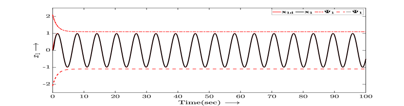
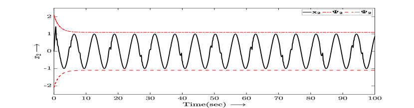
Figure 1: Output tracking and boundedness performance of $x_{1}$.

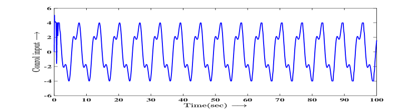
Figure 2: State trajectory and boundedness performance of $x_{2}$.

Figure 3: The control input signal.

VII Conclusion

A control strategy for a nonlinear system with symmetrical and time-varying state restrictions has been proposed. By implementing the proposed approach, no state violates its constraints, and the output follows the desired trajectory asymptotically. The simulation study validated the proposed control scheme’s efficacy.

References

- [1] K. P. Tee, S. S. Ge, and E. H. Tay, “Barrier lyapunov functions for the control of output-constrained nonlinear systems,” Automatica, vol. 45, no. 4, pp. 918 – 927, 2009.
- [2] D. Mayne, J. Rawlings, C. Rao, and P. Scokaert, “Constrained model predictive control: Stability and optimality,” Automatica, vol. 36, no. 6, pp. 789 – 814, 2000.
- [3] D. E. Kirk, Optimal Control Theory: An Introduction. Dover, 2016.
- [4] Y. Liu, L. Ma, L. Liu, S. Tong, and C. L. P. Chen, “Adaptive neural network learning controller design for a class of nonlinear systems with time-varying state constraints,” IEEE Trans. Neural Netw. Learn. Syst., pp. 1–10, 2019.
- [5] B. Cui, Y. Xia, K. Liu, and G. Shen, “Finite-time tracking control for a class of uncertain strict-feedback nonlinear systems with state constraints: A smooth control approach,” IEEE Trans. Neural Netw. Learn. Syst., pp. 1–13, 2020.
- [6] D. Li and D. Li, “Adaptive tracking control for nonlinear time-varying delay systems with full state constraints and unknown control coefficients,” Automatica, vol. 93, pp. 444 – 453, 2018.
- [7] X. Huang, Y. Song, and J. Lai, “Neuro-adaptive control with given performance specifications for strict feedback systems under full-state constraints,” IEEE Trans. Neural Netw. Learn. Syst., vol. 30, pp. 25–34, Jan 2019.
- [8] D. Li, Y. Liu, S. Tong, C. L. P. Chen, and D. Li, “Neural networks-based adaptive control for nonlinear state constrained systems with input delay,” IEEE Trans. Cybern., vol. 49, pp. 1249–1258, April 2019.
- [9] J. Qiu, K. Sun, I. J. Rudas, and H. Gao, “Command filter-based adaptive nn control for mimo nonlinear systems with full-state constraints and actuator hysteresis,” IEEE Trans. Cybern., pp. 1–11, 2019.
- [10] D. Li, S. Lu, and L. Liu, “Adaptive nn cross backstepping control for nonlinear systems with partial time-varying state constraints and its applications to hyper-chaotic systems,” IEEE Trans. Syst., Man, and Cybern.: Syst., pp. 1–12, 2019.
- [11] C. Xi and J. Dong, “Adaptive neural network-based control of uncertain nonlinear systems with time-varying full-state constraints and input constraint,” Neurocomputing, vol. 357, pp. 108 – 115, 2019.
- [12] Y.-D. Song and S. Zhou, “Tracking control of uncertain nonlinear systems with deferred asymmetric time-varying full state constraints,” Automatica, vol. 98, pp. 314 – 322, 2018.
- [13] Y. Sun, S. Gao, L. Ning, H. Dong, and B. Ning, “Output tracking control of strict-feedback non-linear systems under asymmetrically bilateral and time-varying full-state constraints,” IET Control Theory Applications, vol. 14, no. 1, pp. 156–164, 2020.
- [14] D. Li, C. L. P. Chen, Y. Liu, and S. Tong, “Neural network controller design for a class of nonlinear delayed systems with time-varying full-state constraints,” IEEE Trans. Neural Netw. Learn. Syst, vol. 30, pp. 2625–2636, Sep. 2019.
- [15] Y. Liu, M. Gong, L. Liu, S. Tong, and C. L. P. Chen, “Fuzzy observer constraint based on adaptive control for uncertain nonlinear mimo systems with time-varying state constraints,” IEEE Trans. Cybern., pp. 1–10, 2019.
- [16] P. K. Mishra, N. K. Dhar, and N. K. Verma, “Adaptive neural-network control of mimo nonaffine nonlinear systems with asymmetric time-varying state constraints,” IEEE Trans. Cybern., pp. 1–13, 2019.
- [17] Y. J. Liu and S. Tong, “Barrier lyapunov functions for nussbaum gain adaptive control of full state constrained nonlinear systems,” Automatica, vol. 76, pp. 143 – 152, 2017.
- [18] S. S. Ge and J. Wang, “Robust adaptive tracking for time-varying uncertain nonlinear systems with unknown control coefficients,” IEEE Trans. Autom. Control, vol. 48, pp. 1463–1469, Aug 2003.
- [19] Y. J. Liu, J. Li, S. Tong, and C. L. P. Chen, “Neural network control-based adaptive learning design for nonlinear systems with full-state constraints,” IEEE Trans. Neural Netw. Learn. Syst., vol. 27, pp. 1562–1571, July 2016.
- [20] Y. J. Liu, S. Tong, C. L. P. Chen, and D. J. Li, “Adaptive nn control using integral barrier lyapunov functionals for uncertain nonlinear block-triangular constraint systems,” IEEE Trans. Cybern., vol. 47, pp. 3747–3757, Nov 2017.
- [21] Y. J. Liu, S. Lu, D. Li, and S. Tong, “Adaptive controller design-based ablf for a class of nonlinear time-varying state constraint systems,” IEEE Trans. Syst., Man, and Cybern.: Syst., vol. 47, pp. 1546–1553, July 2017.
- [22] R. D. Nussbaum, “Some remarks on a conjecture in parameter adaptive control,” Systems and Control Letters, vol. 3, no. 5, pp. 243–246, 1983.
- [23] B. Ren, S. S. Ge, K. P. Tee, and T. H. Lee, “Adaptive neural control for output feedback nonlinear systems using a barrier lyapunov function,” IEEE Trans. Neural Netw., vol. 21, pp. 1339–1345, Aug 2010.