Obvious Independence of Clones

Abstract

The Independence of Clones (IoC) criterion for social choice functions (voting rules) measures a function’s robustness to strategic nomination. However, prior literature has established empirically that individuals cannot always recognize whether or not a mechanism is strategy-proof and may still submit costly, distortionary misreports even in strategy-proof settings. The intersection of these issues motivates the search for mechanisms which are Obviously Independent of Clones (OIoC): where strategic nomination or strategic exiting of clones obviously have no effect on the outcome of the election. We examine three IoC ranked-choice voting mechanisms and the pre-existing proofs that they are independent of clones: Single Transferable Vote (STV), Ranked Pairs, and the Schulze method. We construct a formal definition of a voting system being Obviously Independent of Clones based on a reduction to a clocked election by considering a bounded agent. Finally, we show that STV and Ranked Pairs are OIoC, whereas we prove an impossibility result for the Schulze method showing that this voting system is not OIoC.

1 Introduction

On November 6th, 1934, Oregonians took to the polls to elect their state’s 28th governor. Beforehand, in a aggressively contested primary, State Senator Joe E. Dunne narrowly defeated Peter Zimmerman. In the subsequent general election, each candidate received the following share of votes [Sec21]:

Charles H. Martin	Peter Zimmerman	Joe E. Dunne
116,677	95,519	86,923

After losing in the Republican primary, Peter Zimmerman had decided to run in the general election as an independent. Zimmerman and Dunne collectively won nearly $60\%$ of the vote, but as individuals, neither managed to edge out the Democratic candidate. The above motivates the following question: How can we make sure that similar candidates in an election do not split the vote, leading to a candidate who is least preferred by the majority of voters winning the election?

This so-called “spoilage” effect motivated T. N. Tideman to formulate the criterion known as Independence of Clones (IoC) in 1987, which ensures that the addition of a candidate with similar policy inclinations will not spoil the election [Tid87]. Intuitively, we would like to ensure that the winner of an election does not change due to the addition of a non-winning candidate who is similar to the winner. Tideman introduced a new voting rule, Ranked Pairs, that satisfies the IoC criterion. Since then, other pre-existing voting rules have been shown to be IoC, such as Single Transferable Vote (STV). The Australian House of Representatives has been using STV since the early 20th century [BL07]. Markus Schulze introduced in 2010 the so-called Schulze method, which he proved to be IoC [Sch11]. The Schulze method has been adopted for all referendums in the town of Silla, Spain as well as in dozens of organizations including the IRC Council for the Operating System Ubuntu [Sch18].

The solution to the spoilage effect then becomes to switch all voting systems to ones that are IoC. However, it is not immediately clear that the average voter or candidate would be convinced that, in switching to one of these methods, the election systems would become impervious to the spoilage effect. As such, even after switching to an IoC rule, a non-believing candidate may still drop out of the election early due to an abundance of caution. Moreover, even a savvy candidate may recognize that many voters will not be willing or able to follow the formal reasoning for why a voting method is independent of clones. As a result, the savvy candidate may still drop out to avoid being blamed by their voter base for a lost election, thus diminishing their chance to hold future elected office.

This motivates examining the obviousness of a mechanism: i.e., how easy it is to “expose” a certain property and make it is easy to understand why the property is indeed satisfied. [Li17] first defined the concept of Obvious Strategy-Proofness, which applies this idea to the property of strategy-proofness (SP). The paper is similarly motivated by the fact that, as noted in the example above, the benefits of a given mechanism’s particular properties are often only accrued when agents understand said property and believe the mechanism satisfies said property. For example, if agents misreport their true rankings for the Gale-Shapley matching algorithms, the results might be suboptimal. Understanding why a mechanism satisfies a property often requires mathematical maturity, time investment, and/or a series of “what if” reasoning steps that are difficult for what Li defines as a cognitively limited agent. This is understood to be an agent who is unable or unwilling to perform contingent reasoning.

Namely, in order for an agent to verify a given mechanism is SP, they may need to reason through what the other agents would do conditioning on their own action. They would then need to reason about how they could best respond to their opponents’ best response, and so on. In an OSP mechanism, it is clear at each step which decision an agent should make, regardless of what the other agent will play at any point down the line.

Intuitively, the IoC criterion requires a similar type of “what if” reasoning. Namely, to verify IoC we ask agents to walk through the steps of a voting rule pretending that there is a clone, and then compare that outcome to the outcome without said clone. Inspired by Li’s work, we introduce the original concept of Obvious Independence of Clones (OIoC). For it, we borrow from Li’s comparison of two mechanisms that when given the same set of private values always return the same allocation and the same payment; i.e., second price sealed bid auctions, which are not OSP, and ascending clock auctions, which are OSP. We use this comparison as motivation to define a clocked election, which is our adaptation of Li’s notion of a personal clock auction to the setting of voting rules by inducing rounds. The definition of clocked election employs our notion of a bounded agent, who acts as a witness during the execution of the protocol.

1.1 Overview

Section 2 introduces pre-existing literature on social choice functions and the Independence of Clones criterion. Section 3 introduces original definitions for a clocked election and a bounded agent. Using these definitions, we formally define a test for determining whether or not a mechanism is Obviously Independent of Clones, based on a reduction to a clocked election with a bounded agent as a witness. We then use this test in Sections 4.1 and 4.2 to establish reductions of the STV and Ranked Pairs voting rules to clocked elections, proving that both voting rules are Obviously Independent of Clones. Section 4.3 establishes an impossibility result, showing that there is no way of transforming Schulze into a clocked election and, therefore, the Schulze method cannot be Obviously Independent of Clones. In Section 5, we discuss implications for future research.

1.2 Related Work

Independence of Clones (IoC). The literature around Independence of Clones dates back to the introduction of the term by [Tid87]. More recently, [EFS10, EFS11] analyze the structure of clone sets as well as the computational difficulty of manipulating non-IoC voting rules via the addition or deletion of clones under different preference profiles. [FBC14] axiomatically define run-off voting rules and prove that the Single Transferrable Vote (STV) rule is the only one to satisfy the IoC criterion. [PX12] discuss the computational complexity of other forms of manipulating well-known IoC voting rules such as the Schulze method and Ranked Pairs.
Obvious Strategy-Proofness (OSP). The literature surrounding obvious strategy-proofness (OSP) is relatively new. As defined by [Li17], an obviously strategy proof mechanism is one that has an equilibrium in obviously dominant strategies, which are strategies where the best possible outcome of deviating is worse than the worst possible outcome of not deviating. Li also provides the behavioral interpretation behind this definition: a strategy is obviously dominant if and only if a cognitively limited agent can recognize it as weakly dominant. We further summarize Li’s definitions in Appendix B. Our definition of a bounded agent used in Section 3 to formalize OIoC is motivated by Li’s definition of a cognitively limited agent.

After being introduced by Li, OSP mechanisms have become the foundation for a robust set of literature that extends existing work on strategy-proofness. [GL21] give a polynomial time algorithm for determining if a voting rule can be implemented as an obviously strategy-proof mechanism. [AG18] prove that stable matching mechanisms are not obviously strategy-proof. [FV17] show that in the machine scheduling and facility location games, OSP-implementation introduces a significant approximation cost. [Tro19] shows that for top trading cycles, OSP-implementation requires an acyclicity condition. Very recently, [GHT22] investigate different ways to describe the same strategy-proof social-choice rule to participants so that strategy-proofness is easier to see, and perform experiments with real participants to test their understanding of a mechanism given the different descriptions.

2 Preliminaries

2.1 Model

We consider a finite set of voters $N=\{1,\ldots,n\}$ and a finite set of candidates $A$ with $|A|=m$. Each voter $i\in N$ has a strict ranking $\sigma_{i}\in\mathcal{L}$ over the candidates in $A$. A preference profile $\boldsymbol{\sigma}\in\mathcal{L}^{n}$ consists of the rankings of all voters and represents an election instance. We often represent $\boldsymbol{\sigma}$ as a matrix with each column being the ranking of a single (or, if specified, a set of) voters with the top entry being the favorite candidate. A voting rule (or social choice function) is a function $f\colon\mathcal{L}^{n}\rightarrow A$ that given a preference profile $\boldsymbol{\sigma}$, outputs the winner of the election.

2.2 Voting Rules Considered in this Paper

Plurality Voting: In plurality voting ($f_{PV}$), the winner is given by the candidate who receives the most first-place votes; i.e., $f_{PV}$ maps $\boldsymbol{\sigma}$ to the candidate that appears the most on the first row of $\boldsymbol{\sigma}$.

Borda Count: In Borda count ($f_{BC}$), each voter gives $m-k$ “Borda points” to the alternative placed in the $k$-th position, where $m$ is the number of alternatives. $f_{BC}$ maps $\boldsymbol{\sigma}$ to the candidate with the most Borda points.

Single Transferable Vote: In Single Transferable Vote (STV) ($f_{STV}$), we run an iterative algorithm on $\boldsymbol{\sigma}$ to determine the winner. At each round, if no candidate has majority (more than half of the plurality votes), the candidate with the fewest plurality votes is eliminated, and these votes are transferred to the candidate named second in the ranking [Tid87]. Eventually, a candidate secures majority, and becomes the winner.

While STV is the simplest IoC voting method that we consider, it is not Condorcet consistent (i.e., we can construct preference profiles in which a candidate wins against every other candidate in a head-to-head contest, but is not the STV winner nevertheless). For this reason, we turn to the following two graph-based algorithms: Ranked Pairs and the Schulze method, which are both Condorcet consistent and IoC [Tid87, Sch11].

Ranked Pairs: The Ranked Pairs (RP) ($f_{RP}$) voting system was developed by [Tid87] specifically to satisfy the Independence of Clones criterion. While Tideman’s original formulation takes in a preference profile and returns a complete ranking of alternatives, for the purposes of this paper, we will be dealing with a simplified version of Ranked Pairs which takes in the same prefernce profile and simply returns the winner of the election. On input $\boldsymbol{\sigma}$, $f_{RP}$ does as follows:

1. For convenience, label the candidates in $A$ as $\{a_{i}\}_{i\in[m]}$. Based on the preference profile $\boldsymbol{\sigma}$, construct the so-called majority matrix $M$, whose $ij$ component is equal to the difference between the number of voters who rank $a_{i}$ ahead of $a_{j}$ and the number of voters who rank $a_{j}$ ahead of $a_{i}$. Accordingly, $M$ is an anti-symmetric matrix, and thus $M[a_{i},a_{j}]=-M[a_{j},a_{i}]$.

2. Sort the positive majorities in $M$ in decreasing order of magnitude. Let $\mathcal{L}$ be the list containing the pairs $(a_{i},a_{j})$ in this order.

3. Construct a directed graph $G$ by iterating through the pairs in $\mathcal{L}$ in order. For each pair $(a_{i},a_{j})$, add a directed edge $e_{ij}$ from node $i$ to $j$ if $M[a_{i},a_{j}]>M[a_{j},a_{i}]$, and from $j$ to $i$ otherwise. If $e_{ij}$ creates a cycle in $G$, remove the edge.

4. The winner of the election is the candidate that corresponds to the source node of $G$. [Tid87] shows that the source of the graph exists and is unique. To illustrate, consider an example run of the Ranked Pairs algorithm in Appendix D.2.

The Schulze method: The Schulze method ($f_{SM}$) was introduced by [Sch11] as a new monotone, clone-independent, and Condorcet-consistent single-winner election method. On input voter profile $\boldsymbol{\sigma}$, $f_{SM}$ does as follows:

1. Based on the voter profile, construct the so-called pairwise matrix $P$, whose $ij$ component is equal to the number of voters who rank $a_{i}$ ahead of $a_{j}$.

2. Construct a graph $G$ where node $i$ corresponds to candidate $a_{i}$ as follows: For each pair of candidates $(a_{i},a_{j})$, add a directed edge $e_{ij}$ from node $i$ to $j$ if $P_{ij}>P_{ji}$, and from $j$ to $i$ otherwise. The weight of the edge, denoted $w(e_{ij})$, is equal to $\max\{P_{ij},P_{ji}\}$.

3. For each path in $G$ from candidate $a_{i}$ to $a_{j}$, the strength of the path is defined as the minimum of the weights of all edges in the path. For each pair of indices $i,j$, we want to maximize the weight of the minimum-weight edge in the path from $a_{i}$ to $a_{j}$. We can compute this, for example, with the Floyd-Warshall algorithm [Sch11].

4. After computing the strengths of the strongest paths, we construct the strength matrix $S$, whose $ij$ component is equal to the strength of the strongest path from $a_{i}$ to $a_{j}$.

5. Now we need to examine the entirety of matrix $S$. For each pair of candidates $(a_{i},a_{j})$, compare $S[a_{i},a_{j}]$ to $S[a_{j},a_{i}]$. If $S[a_{i},a_{j}]>S[a_{j},a_{i}]$, then $a_{i}>a_{j}$ in the final ranking, and vice versa. After all pairwise comparisons, the final ranking of candidates has been determined. The winner of the Schulze method corresponds to the top-ranked candidate.

   As proven by [Sch11], a winner always exists and is unique. Comparing the Schulze method to Ranked Pairs, we remark that we can construct the pairwise matrix from the majority matrix and viceversa. An important aspect to remark about Schulze is the fact that the final ranking is unique, no matter the order in which we compare the candidates in the strength matrix. This point will become relevant when we examine our proposed notion of Obvious Independence of Clones. For an example of Schulze’s algorithm, see Appendix D.3.

2.3 The Independence of Clones Metric

Definition 2.1 (Set of clones [Tid87]).

A proper subset of two or more candidates, $K\subsetneq A$, is a set of clones if no voter ranks any candidate outside of $K$ as either tied with any element of $K$ or between any two elements of $K$.

Intuitively, this captures the idea that the voters’ rankings are consistent with the hypothesis that the candidates in $K$ are close to one another in some shared perceptual space. For example, in the following voter profile $\boldsymbol{\sigma}$, candidates $b$ and $c$ are clones:

2	4	7	9	13
Voters	Voters	Voters	Voters	Voters
a	a	b	c	d
b	c	c	b	a
c	b	d	d	b
d	d	a	a	c

Definition 2.2 (Independence of Clones [Tid87]).

Recall that a voting rule maps individuals’ preference orderings to an element in the set of individual alternatives. We say a voting rule is Independent of Clones (IoC) if and only if the following two conditions are met when clones are on the ballot:

1. A candidate that is a member of a set of clones wins if and only if some member of that set of clones wins after a member of the set is eliminated from the ballot.

2. A candidate that is not a member of a set of clones wins if and only if that candidate wins after any clone is eliminated from the ballot.

In other words, deleting one of the clones must not increase or decrease the winning chance of any candidate not in the set of clones. This is a desirable property in voting rules, since it imposes that the winner must not change due to the addition of a non-winning candidate who is similar to a candidate already present. This prevents candidates influencing the election by nominating new candidates similar to them or their opponents.

Note that we use an approach to voting rules that cannot produce ties. To adjust for ties, we can expand this definition of voting rule to one that returns a subset of alternatives, in which case the IoC criterion becomes that deleting a clone must not affect the probability of a member of the set of clones being in the set of winners. Alternatively, we can keep the above criterion and definitions, and say that our voting rule decides ties uniformly at random. For simplicity, in the remainder of this paper we assume ties do not exist.

It is worth noting that for voting rules that are not independent of clones, the impact of having clones on the chances of winning can vary. For instance, among the voting rules listed in Section 2.2, both Plurality and Borda Count are not independent clones. However, Plurality is “clone-negative” (i.e., having clones decreases the chances of a candidate winning) while Borda Count is “clone-positive” (i.e., having clones increases the chances of a candidate winning). Examples demonstrating this difference can be found in Appendix C.1. STV, Ranked Pairs, and the Schulze method, on the other hand, are all IoC. The proof showing that STV is IoC is provided in Appendix A.3, while the proofs for Ranked Pairs and the Schulze method can be found in the papers by [Tid87, §V] and [Sch11, §4.6], respectively.

3 Obvious Independence of Clones (OIoC)

Motivated by Li’s formalization of the notion of Obviously Strategy-Proof (OSP) mechanisms, we adapt some of his key definitions and insights to the setting of voting rules and to the property of Independence of Clones. Li introduces three notions that allow him to prove that certain notions are equivalent to OSP: $i$-indistinguishability [Li17, Def. 9, Thm. 1], bilateral commitments [Li17, Def. 12, Thm. 2], and personal-clock auctions [Li17, Def. 15, Thm. 3].

Bounded agents. As alluded to in Section 1 (and as explained in more detail in Appendix B), $i$-indistinguishability captures the idea of a cognitively-limited agent being incapable of engaging in contingent reasoning. For our purposes, we need to modify this definition to what we call a bounded agent. We first introduce the formal definition and provide further intuition in the explanation following definitions 3.2 and 3.3. As in our conceptual explanation for our definition of OIoC introduces the role of a cheater (which is inspired by the role of an adversary in cryptographic protocols), we view the bounded agent as a witness during the clocked election protocol (Definition 3.2). This explains why the Definition 3.1 has a cryptographic flavor (more concretely, we take inspiration from the notion of simulation-based security [Lin17]). We also draw inspiration from the definition of Turing Machines in complexity theory.

Definition 3.1 (Bounded agent).

Let $f$ be a function and let $\pi$ be a one-party protocol for computing $f$. The $\mathsf{view}$ of Agent $i$ during the execution of $\pi$ on input $x$ is denoted by $\mathsf{view}^{\pi}_{i}(x)$ and it equals the transcript $(x,r^{i}_{1},\ldots,r^{i}_{t};m_{1},\ldots,m_{t})$, where $r^{i}_{j}$ equals the contents of the $i$th party’s internal computations at the $j$-th step of the execution, and $m_{j}$ corresponds to the state of the protocol at the $j$-th step of its execution. Then, we say that an agent $B$ is bounded if it satisfies the following properties:

1. For any arbitrary agent $A$ of possibly unbounded computational complexity who is executing $\pi$, the bounded agent $B$ must concurrently receive the full transcript of the execution of $\pi$, including any internal side computations performed by agent $A$. That is, $\mathsf{view}^{\pi}_{A}(x)=\mathsf{view}^{\pi}_{B}(x)$.

2. $B$ has constant computational power (i.e., can perform at most $C$ operations for some $C=O(1)$).

3. The bounded agent $B$ has a tape of infinite length on which it can perform read and write operations. This means that $B$ is able to read the transcript generated during the execution of the protocol, while being unable to read any unaccessed data. We remark that this read and write access is granted on top of $B$’s computational power; otherwise, this condition would not be achievable under $B$’s constant computational power (Property 2).

4. $B$ has access to the description of $f$; i.e., $B$ has the necessary information to execute $\pi$, but does not have the necessary computing power to do so (by Property 2).

Before we turn to the definition of a clocked election, we show an example of what Property 2 in Definition 3.1 entails. Consider the case where $f$ corresponds to the Schulze method. That is, on input a preference profile $\boldsymbol{\sigma}$ for voters $N$ and candidates $A$, $f(\boldsymbol{\sigma})$ returns the Schulze winner $a\in A$.

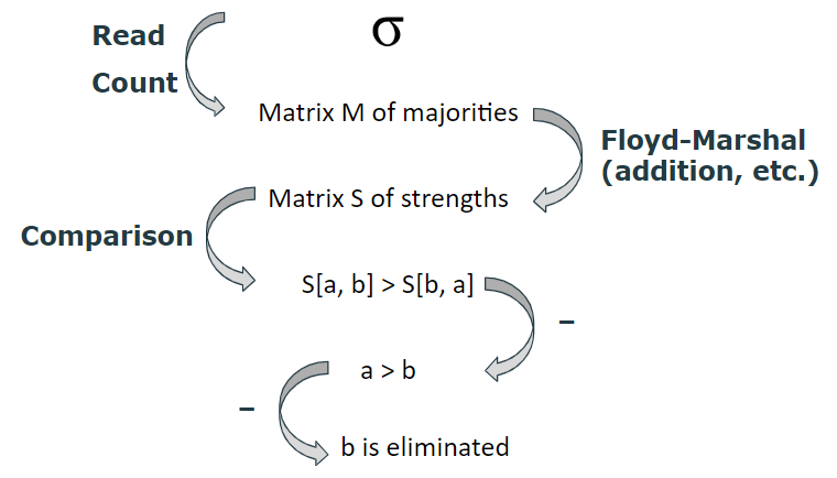
Figure 1: Simplified Schulze diagram.

By Property 2 (i.e., that $B$ has constant computational power), the bounded agent $B$ cannot read the entirety of $\boldsymbol{\sigma}$ for an arbitrary $\boldsymbol{\sigma}$ (which can be of any length that depends asymptotically on $n$), run the Floyd-Warshall algorithm, or do all of the pairwise comparisons. However, upon reading that $S[a,b]>S[b,a]$ from the logs of the computation (being executed by an agent $A$), $B$ is able to infer that $S[a,b]>S[b,a]$ implies $a>b$ in the final ranking (where $a,b$ denote two candidates in $A$ and $S$ the strength matrix as defined in Section 2.2), and that this in turn implies that $a$ eliminates $b$.

Clocked Election. After careful examination, we found that the idea of the personal clock auction was the most natural to adapt to our setting of voting rules. As discussed in Section 1 and Appendix B, the clock auction is OSP while the sealed second price auction is not, demonstrating that two different implementations with the same reduced normal form game can differ in whether they are OSP or not. In fact, Li further generalizes this notion by proving that a game has an OSP implementation if and only if it can be reduced to what he calls a “personal-clock auction” [Li17, Thm. 3]. The definition for “personal-clock auction” is broadly a generalization of the clock auction in which every player has a set of ‘quitting’ actions at each round [Li17, Def. 15]. Motivated by this theorem, we provide the following definition:

Definition 3.2 (Clocked Election).

A Clocked Election for a voting rule $f$ is a protocol $CE$ that takes as input a preference profile $\boldsymbol{\sigma}$ for voters $N$ and candidates $A$ and iteratively fills an ordered list of ‘eliminated’ candidates $F$ (where $F_{i}$ is the state of the list after $i$ iterations and hence $F_{m-1}$ is the final list) such that the following conditions hold:

1. For any set of clones $K\subset A$ and any $d\in K$, let $F^{\prime}$ be the list that $CE$ would output on input $\boldsymbol{\sigma}\setminus({K\setminus\{d\}})$ (i.e., the preference profile with all the clones removed except for $d$). Then, for all $i\in\{1,\ldots,m-1\}$:

   • If $\exists g\in K$ such that $g\notin F_{i}$, then $F_{i}\setminus K=F^{\prime}_{j}$ for some $j\in\{0,1,...,m-1\}$ (where $F^{\prime}_{0}:=\emptyset$).

   • Otherwise, let $g^{*}\in K$ be the clone with the largest index in $F_{i}$. Then $F_{i}\setminus(K\setminus\{g^{*}\})$ with $g^{*}$ replaced with $d$ is equal to $F^{\prime}_{j}$ for some $j\in\{0,1,\ldots,m-1\}$.

2. Let $\mathcal{L}$ denote all the logs of the computation up to $F_{i}$ for $i<m-1$, and let $\Sigma_{\mathcal{L}}$ denote the set of all possible preference profiles $\boldsymbol{\sigma}$ for voters $N$ and candidates $A$ that lead to $\mathcal{L}$. A bounded agent (as defined in Definition 3.1) who is given $\mathcal{L}$ as input cannot output $a\in A$ such that $a\notin F_{i}$ but $a\in F_{m-1}$ with probability 1 over $\Sigma_{\mathcal{L}}$. That is, there must exist at least one $\boldsymbol{\sigma}\in\Sigma_{\mathcal{L}}$ for which the bounded agent does not output the correct $a$. In particular, the bounded agent does not have access to any entries from $\boldsymbol{\sigma}$ that the protocol has not used yet. Moreover, the memory of the bounded agent is reset at each iteration of the clocked election. In other words, the bounded agent cannot use any results from any of its own computations in previous iterations.

3. $CE$ satisfies neutrality. That is, permuting the rows and columns $\boldsymbol{\sigma}$ before the protocol is run should result in the same permutation on the output list $F$.

4. $A\setminus F_{m-1}=\{f(\boldsymbol{\sigma})\}$.

Along with the definition for bounded agent above, this definition provides all the necessary pieces to formalize our definition for Obviously Independent of Clones:

Definition 3.3 (Obvious Independence of Clones).

A social choice function $f$ is Obviously Independent of Clones (OIoC) if and only if it can be reduced to a clocked election.

Before applying this definition to various voting rules, it is worthwhile to elaborate on the purposes of each of the four conditions stated in Definition 3.2.

Intuition for Condition 1. Motivated by the personal clock auction definition by Li, Condition 1 imposes the notion of rounds onto the voting rule, requiring that its implementation can be reduced to steps in which one candidate is eliminated at a time, and the order in which the candidates are eliminated is stored in the list $F_{i}$ at the $i$th iteration. Moreover, this condition ensures that at any point during the implementation, removing all but the longest-lasting clone from the list of eliminated candidates does not change the order one would have gotten if they had run the protocol with these clones removed. This provides understanding for why the protocol is “obviously” independent of clones: once a clone does get eliminated, it follows immediately at that round (and in following rounds) that they never really influenced the execution of the voting rule, so every step of the protocol (including the output) is as if they had never run. Another way of looking at this is that even if we allowed the clones to forfeit and leave the election mid-way at any of the rounds, we would not have to rerun the protocol from start, as all of the lists with the forfeited clone removed would be identical to running the algorithm without the clone.

Intuition for Condition 2. Condition 2 rules out trivial reductions from the definition. Suppose that we have an adversary with arbitrarily powerful computational capacity who is trying to reduce an independent of clones voting rule (that outputs a final ranking of the candidates) into a clocked election. Using its unlimited computational capacity, the adversary could simply run the voting rule on $\boldsymbol{\sigma}$ using any implementation and get the resulting ranking as an output (e.g., without loss of generality suppose that it is $a>b>c>d$ is the final ranking of the candidates after running the voting rule) and then start forming the list of eliminated candidates by inputting the ranking from end to start (e.g. adding $d$, then $c$, then $b$, and then $a$). Since the voting rule is independent of clones, if the adversary ran the algorithm with clones, all of the clones would appear consecutively in the resulting ranking (e.g. $a>b>c>c_{1}>d$ if $c$ was cloned), and hence the list that the adversary would form would indeed have the same order when the clones are removed. This is undesirable, as it would permit all independent of clones voting rules that output a final ranking to be trivially obviously independent of clones.

We could prevent this by limiting the complexity of the reduction to the clocked election, hence restricting the computing power of the adversary, but this would cause our definition of OIoC only depend on the complexity of the voting rules (e.g., the Schulze method has a higher runtime complexity than Ranked Pairs because of the step running the Floyd-Warshall algorithm). However, this would not be the right approach when defining OIoC, given that it would reduce complexity of understanding to complexity of computation, which is not necessarily true. In other words, this approach would define obviousness of a mechanism in terms of the amount of computation required to run it. This is not the notion of obviousness that we want to capture; instead, we introduce a bounded agent (see Definition 3.1) in order to ensure that the adversary does not “cheat.” That is, when pausing the reduction at any step $i$, the bounded agent cannot read new information from $\boldsymbol{\sigma}$ or perform new computations other than $O(1)$ operations, but is allowed to read the logs of the reduction up until that point. For example, if the adversary is trying to perform the trivial reduction explained above (coming up with the final ranking and then filling the list of eliminated candidates one by one), the bounded agent would have access to this result, thus constructing $F_{i+1},\ldots,F_{m-1}$ on its own, violating the definition.

Intuition for Condition 3. Condition 3 is intended to protect against any strategy in which the adversary exploits arbitrary orderings of the candidates. For instance, the adversary could first detect all the groups of clones by reading the entirety of $\boldsymbol{\sigma}$ and come up with an arbitrary ordering of candidates in which the clones appear right next to each other. If the voting method induces a certain strength or score parameter that the final ranking is based on, then the adversary could simply perform pairwise comparisons of candidates in the arbitrary order it has set (eliminating the one with the lower score), and hence ensure that the order of elimination with or without clones the same, which does not align with the formulation of a clocked election with rounds. Note that Condition 2 is not sufficient to protect against such strategies as the bounded agent is incapable of comparing magnitudes of numbers in constant time. Without Condition 3, all independent of clones methods that induce a strength or score metric would be OIoC.

Intuition for Condition 4. Condition 4 simply ensures that the clocked election that the voting rule is reduced to produces a winner which is consistent with the winner that the voting rule determines.

3.1 Direct consequences of the definition

Proposition 3.4.

OIoC implies IoC.

The proof can be found in Appendix C.1. This shows that OIoC is a stronger property than IoC, which is what we would expect.

Proposition 3.5.

Without Condition $\boxed{2}$, IoC implies OIoC.

The proof can be found in Appendix C.2. This formalizes the idea that a bounded agent is required against adversarial reductions that would render every IoC rule trivially OIoC.

4 Analysis of IoC Voting Rules for OIoC

We now look at the application of the definition of OIoC to various voting rules that are independent of clones: STV, Ranked Pairs, and the Schulze method.

4.1 STV

In STV, the notion of rounds required by Definition 3.2 is already present in the natural implementation of the voting rule: in each round, the candidate with the least plurality votes is eliminated. Hence, we can easily define the following protocol:

Definition 4.1 ($CE_{STV}$ Protocol).

Given input $\boldsymbol{\sigma}$ for candidates $A$ and voters $N$, $CE_{STV}$ performs the following procedure:

Step 1: Read only the top row of $\boldsymbol{\sigma}$, counting the votes for each candidate. Pick the candidate with the least number of votes on the top row (say $a_{1}$), and declare $F_{1}=\{a_{1}\}$. Delete all the entries of the top row of $\boldsymbol{\sigma}$ that has $a_{1}$ as its entry and replace it by NULL produce new preference profile $\boldsymbol{\sigma}_{1}$ (i.e. for all $i\in\{1,\ldots,|N|\}$, $\boldsymbol{\sigma}^{\prime}_{1i}=\begin{cases}\textbf{NULL}&\text{ if }\boldsymbol{\sigma}_{1i}=a_{1},\\ \boldsymbol{\sigma}_{1i}&\text{ otherwise}.\end{cases}$

Step $\boldsymbol{i}$ (for $i\in\{2,\ldots,m-1\}$): Once step $i-1$ is complete, count the votes from the top non-NULL entry of each column of $\boldsymbol{\sigma}_{i-1}$ (by starting from the top of each column and moving the next entry only if the entry is NULL). Determine the candidates with the least number of votes among these “top” votes (say $a_{i}$) and declare $F_{i}=F_{i-1}\cup\{a_{i}\}$ (where $a_{i}$ is added to the end). For each of the columns that have $a_{i}$ as their top non-NULL entry, change this entry to NULL to produce $\boldsymbol{\sigma}_{i}$ and move to the next entry in the column. If the candidate in the next entry is in $F_{i}$, change this entry to NULL as well and keep moving to the next entry until either a candidate not in $F_{i}$ is encountered or the column is all NULL.

Note that after step $m-1$, $\boldsymbol{\sigma}_{m-1}$ has only NULL as its entries and the $F_{m-1}$ has all but one candidate.

Theorem 4.2.

$CE_{STV}$ is a Clocked Election for STV.

The proof can be found in Appendix C.3.

Corollary 4.3.

STV is Obviously Independent of Clones.

4.2 Ranked Pairs

Next, we analyze how Ranked Pairs (RP) can be reduced to a clocked election. For this voting rule, the notion of rounds can be induced using the order in which we add the edges to the graph (without creating a cycle). A key observation is that once any vertex has an incoming edge locked in the graph, the corresponding candidate no longer has the chance of being the winner (as the winner will be a source of the final graph) and hence can be added to the list $F$. Based on this idea, we define the following protocol:

Definition 4.4 ($CE_{RP}$ Protocol).

Given input $\boldsymbol{\sigma}$ for candidates $A$ and voters $N$, $CE_{RP}$ performs the following procedure:

Step 0: For each $a,b\in A$, read every column of $\boldsymbol{\sigma}$ in order to count the number of voters that prefer $a$ over $b$ and viceversa. Use these numbers to fill the majority matrix $M^{(0)}$ where $M^{(0)}_{ab}$ is the number of voters that prefer $a$ over $b$ minus the number of voters that prefer $b$ over $a$. Initialize a graph $G_{0}(V,E_{0})$ where $V=A$ and $E_{0}=\emptyset$.

Step $\boldsymbol{i}$ (for $i\in\{1,\ldots,m-1\}$): Once step $i-1$ is complete, the current graph is $G_{i-1}(V,E_{i-1})$. Query the current majority matrix $M^{(i-1)}$ to find the largest non-NULL entry (say $M^{(i-1)}_{ab}$). First, set $M^{(i)}_{ab}=\textbf{NULL}$ to produce $M^{(i)}$ from $M^{(i-1)}$. Add $(a,b)$ to $E_{i-1}$ to get $G_{i}(V,E_{i})=G_{i}(V,E_{i-1}\cup\{(a,b)\})$ only if it does not create a cycle. Otherwise, repeat by finding the next largest entry in the majority matrix, set it to NULL, check if the corresponding edge creates a cycle, etc. until either an edge not creating a cycle is found and added to $G_{i}(V,E_{i})$ or there are no more non-NULL positive entries in $M^{(i)}$, in which case terminate. Once an edge $(a,b)$ is added to $G_{i}(V,E_{i})$, check if $b$ is in $F_{i-1}$. If $b\notin F_{i-1}$, add it to produce $F_{i}=F_{i-1}\cup\{b\}$ and move to step $i+1$ (or terminate if $i=m-1$). If $b\in F_{i-1}$, repeat this step again with the current $G_{i}(V,E_{i})$ and $M^{(i)}$ until an edge pointing at a vertex not in $F_{i-1}$ is added to $G_{i}(V,E_{i})$, and only then move to step $i+1$.

Note that within a single step $i$, the protocol might add multiple edges to the graph $G_{i}(V,E_{i})$, but by construction it will only eliminate one candidate per step. Hence, at step $m-1$, $F_{m-1}$ has all but one candidate, as desired.

Theorem 4.5.

$CE_{RP}$ is a Clocked Election for Ranked Pairs.

The proof can be found in Appendix C.4.

Corollary 4.6.

Ranked Pairs is Obviously Independent of Clones.

4.3 The Schulze Method

Having shown that both STV and Ranked Pairs are Obviously Independent of Clones, we now present an impossibility result:

Theorem 4.7.

The Schulze method is not Obviously Independent of Clones.

Proof sketch.

The full proof for Theorem 4.7 is provided in Appendix C.5. Here we provide a sketch of the proof.

The critical idea is that unlike STV and Ranked Pairs, in which the notion of rounds can be easily implemented using the elimination of the candidate with the least plurality votes and the addition of the maximum majority edge from $M$, respectively, there is no natural notion of rounds in the Schulze method. Even after the creation of the strength matrix $S$, any protocol implementing the Schulze method must decide on an order in which to compare the strength of the candidates. For instance, a comparison of the type $S[a,b]>S[b,a]$ for $a,b\in A$, conclusively shows that we will have $a>b$ in the final ranking (and hence $b$ can be eliminated). However, once a third candidate $c\in A$ is compared with the previous two, all three of these cases are possible:

• $S[a,c]>S[c,a]$ and $S[b,c]>S[c,b]$ (hence $a>b>c$).

• $S[a,c]>S[c,a]$ and $S[c,b]>S[b,c]$ (hence $a>c>b$).

• $S[c,a]>S[a,c]$ and $S[c,b]>S[b,c]$ (hence $c>a>b$).

Since there is no way to deduct which of these cases will arise without making the said comparisons, the final ranking of the candidates is not linearly formed.

In order to formalize this idea in our proof, we use Condition $$4$$ from Definition 3.2 to confirm that the result of a clocked election for the Schulze method should indeed be consistent with such strength comparisons. We then use Condition $$2$$ to conclude that between two consecutive rounds of the protocol (i.e., between outputting $F_{i-1}$ and $F_{i}$ for any $i\in[m-1]$) there can be at most one new candidate with which strength comparisons are made. This is because a comparison of the type $S[a,b]>S[b,a]$ conclusively confirms that $b\in F_{m-1}$. Hence, if there are two different candidates $c_{1},c_{2}\in A\setminus F_{i-1}$ such that they are both compared in strength to the older candidates before outputting $F_{i}$, there will always be two new candidates that are conclusively eliminated. Therefore, a bounded-time agent that outputs $b\in A$ whenever it sees the comparison $S[a,b]>S[b,a]$ for some $a\in A$ in the logs of the protocol (which can be done in constant time as outlined in Definition 3.1) will always be able to output a non-winner candidate that is not in $F_{i}$, hence disqualifying the protocol. Lastly, we use Conditions $\boxed{1}$ and $\boxed{3}$ to establish that the order in which the candidates are compared in strength cannot be arbitrary and requires the existence of a deterministic function of the pairwise comparison matrix.

Using these conclusions, we complete the proof by producing a family of counterexamples containing what we call “pseudo-clones”: candidates that are not clones but have the same pairwise comparisons to every other candidate, like clones. We show that we can indeed construct a preference profile belonging to this family of examples and that it is impossible for any protocol to fulfill Condition $\boxed{1}$ for all of the instances produced from the original preference profile by cloning a single pseudo-clone. This shows that no protocol running the Schulze method can fulfill all of the conditions of Definition 3.2, and hence the Schulze Method is not OIoC.

∎

5 Conclusion & Future Work

This paper bridges two separate phenomena from computational social choice and mechanism design: the Independence of Clones property of a social choice function and the game-theoretic notion of obviousness. We have formally defined the notion of Obvious Independence of Clones (OIoC) and showed that it captures the intuition of why it is harder to reason about Schulze than STV or Ranked Pairs.

Our formalization, besides demonstrating a mathematical separation between different voting rules, implies a powerful computational advantage: if we can show that a voting rule is OIoC, then we know that if a clone drops the election at any time during the execution of the algorithm, it is not necessary that we re-start the election, and every single step in the algorithm will remain the same, equivalent to the steps produced had the candidate not run. This is demonstrated by the fact that the order of remaining eliminated candidates would be the same with or without that clone.

This paper opens different new lines of work. First, we can consider other voting rules that satisfy the independence of clones criterion and prove whether or not they are also OIoC. Some possibilities include the GOCHA rule and alternative voting [Tid87]. Second, the concept of obviousness can potentially be adapted to many other properties of voting rules, such as monotonicity. Lastly, some of the tools that we develop in the proofs of the paper, such as the notions of bounded agent or pseudoclone, are potentially useful in other settings.

Appendix A Discussion of Independence of Clones

We begin by examining whether the voting rules defined in Section 2.2 satisfy Independence of Clones.

A.1 Plurality Voting

As demonstrated by the historical example in Section 1, we can readily see that plurality does not satisfy IoC. Consider the following voting profile for candidates $a$ and $b$:

62	38
Voters	Voters
a	b
b	a

In this case, the winner of the election is $a$. After introducing a clone $a_{2}$ of $a$, we can obtain the following voting profile:

28	34	38
Voters	Voters	Voters
a	a2	b
a2	a	a2
b	b	a

With the introduction of clone $a_{2}$, we see that the winner is now $b$, who is not part of the set of clones. Thus, the clone of $a$ has negatively impacted $a$.

A.2 Borda Count

We provide an example to show that Borda does not satisfy IoC either. Consider the following voting profile for candidates $a$ and $b$:

62	38
Voters	Voters
a	b
b	a

In this case, candidate $a$ receives 62 Borda points, whereas candidate $b$ receives 38 Borda points. Thus, candidate $a$ wins the election. Next we introduce a clone of $b$, obtaining the following voting profile:

62	38
Voters	Voters
a	b
b	b2
b2	a

Now candidate $a$ receives 124 Borda points, $b$ receives 138 Borda points, and clone $b_{2}$ receives 38 Borda points. Hence, candidate $b$ now becomes the winner. Unlike the plurality example, this is a case where the clone of $b$ has positively impacted $b$. Therefore, the Borda Count is not Independent of Clones. More generally, we can prove the following statement:

Lemma A.1.

Any preference profile in which candidate $a$ wins against candidate $b$ using the Borda count (with an arbitrarily large margin) can be turned into a preference profile in which $b$ wins by adding clones of $b$, given that there is at least one voter that prefers $b$ over $a$.

Proof.

Consider $N$ voters and 2 candidates $a$ and $b$, where $P$ voters prefer $b$ to $a$ and $N-P$ voters prefer $a$ to $b$ (with $P\geq 1$ by assumption). Let $P_{1}(a)$ denote the Borda points obtained by candidate $a$, and let $P_{1}(b)$ denote the Borda points obtained by candidate $b$, where $P_{1}(a)>P_{1}(b)$ without loss of generality. Next we add $Q$ clones of $b$, ranking strictly less than $b$. Then each of the $P$ voters who prefer $b$ to $a$ grants $Q$ additional Borda points to $b$, for a total of $QP$ additional points. Each of the $N-P$ voters who prefer $a$ to $B$ grants $Q$ additional points to $b$ and $Q$ additional points to $a$, for a total of $Q(N-P)$ Borda points. Hence, the new total Borda points after the addition of the clones is $Q(N-P)$ for $a$ and $QN$ for $b$. Then, for any $Q$ such that $Q>\frac{P_{1}(a)-P_{1}(b)}{P}$, we conclude that the winner has been flipped. ∎

A.3 STV

Unlike plurality and Borda count, STV is Independent of Clones. To show this, we adapt the argument presented in Section V of [Tid87].

Lemma A.2.

STV is Independent of Clones.

Proof.

Consider an election with a set of candidates that includes a set of clones $C$. In each individual voter’s ranking, all of the clones must be adjacent. Therefore, at any given moment in the election, if a clone is eliminated and there are other clones remaining, all of its first place votes are reallocated to another clone. Therefore, the number of first-place votes for each of the non-clone candidates is unchanged and the number of first-place votes that the set of clones collectively has is also unchanged. Furthermore, when another candidate is eliminated while some non-empty set of clones $C^{\prime}$ is still in the election, each of the eliminated candidate’s first place votes is either allocated to either a member of $C^{\prime}$ or non-member of $C^{\prime}$. If it is allocated to a non-member of $C^{\prime}$, there is no way of changing $C^{\prime}$ such that it it can change this allocation. Furthermore, if the vote is allocated to a member of $C^{\prime}$, since all of the members of $C^{\prime}$ are adjacent in the ranking, it will always be allocated to a member of $C^{\prime}$ even if $C^{\prime}$ is modified. Therefore, in both of these steps, the set of clones will always have the same number of first place votes in aggregate, no matter the composition of $C$. Hence, if we compare the original election to the election with clones, by the time that all but one of the clones are eliminated, the number of first place votes that the final clone and the other candidates have will be identical to the original election.

Therefore, we conclude that STV is IoC. ∎

For examples illustrating that STV is IoC, see Appendix D.1.

A.4 A Note on Coherence

The following argument is adapted from [Tid87], Section IV.

It is worth observing that given Definition 2.2, there is a trivial composition that can make any non-IoC voting rule one that is IoC. Namely, suppose we first impose a primary between all clone candidates. This allows us to condense a set of clones into a single clone, who will thus not be affected by clones in the general election. In fact, this system is in place in many nations that use plurality voting, which is not IoC (as discussed in Appendix A.1). The above formulation poses several issues. First, it requires a strict primary process, where losing clones are disallowed from running in the general election. Moreover, it requires that primaries be run between sets of clones, which means clones need to be identified priors to voters voting.

Such a formulation also lacks a notion of “coherence”, as shown by the following topological argument against primary voting as a means to insure independence of clones: the domain of an anonymous and homogeneous voting rule can be interpreted as the space spanned by the vectors composed of the number of votes for each candidate. Projecting this set of vectors onto the rational subspace of the unit simplex gives us a topological representation of the intuitive statement that the results can be expressed as a function of the proportion of votes each candidate gets. In this domain, performing a primary where we search for clones and dominant candidates sharply divides the region into two sections: one where there is a clone and one where there is not. These ragged edges undermine the smoothness of our voting rule function, which could be interpreted as a lack of coherence in such two-part voting rules.

Appendix B Obvious Strategy-Proofness

Our initial inquiry on the property of “obviousness” originated from the introduction of Obviously Strategy-Proof Mechanisms (OSP) by [Li17]. As outlined in the introduction, “exposing” the strategy-proofness of the mechanism is important for ensuring that agents rank truthfully, since otherwise the outputs might be suboptimal (e.g., when running the Gale-Shapley matching mechanism). Li captures this notion with the following two definitions:

Definition B.1 (Obviously dominant [Li17]).

A strategy is obviously dominant if, for any deviation, at any information set where both strategies first diverge, the best outcome under the deviation is no better than the worst outcome under the dominant strategy.

Definition B.2 (Obviously strategy-proof (OSP) [Li17]).

A mechanism is obviously strategy-proof (OSP) if it has an equilibrium in obviously dominant strategies.

Li also provides the behavioral interpretation behind this definition: a strategy is obviously dominant if and only if a cognitively limited agent can recognize it as weakly dominant. A cognitively limited agent is understood as someone who is unable to engage in contingent reasoning. This differs from our definition of bounded agent in Section 3, where we need to establish a formal definition of this agent to require some more restrictive properties. The notion of a cognitively limited agent is best described with an example, which is presented by [Li17]. Consider Figure 2 and suppose that Agent 1 has preferences $A\succ B\succ C\succ D$. In mechanism (i), it is a weakly dominant strategy for 1 to play $L$, whereas in mechanism (iii) it is not a weakly dominant strategy for Agent 1 to play $L$. However, if Agent 1 cannot engage in contingent reasoning (i.e., cannot think through hypothetical scenarios), then he cannot distinguish between (i) and (ii). As coined by Li, this means that (i) and (ii) are 1-indistinguishable.

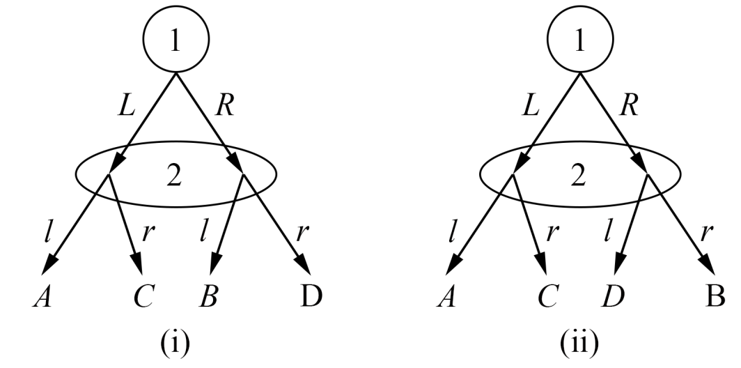
Figure 2: Agent 1 is unable to distinguish between mechanisms 1 and 2 (Fig. 1 in [Li17]).

An illustrative example of the difference between strategy-proofness and Obvious Strategy-Proofness (OSP) is in the comparative analysis of the ascending clock auction and the Second Price Sealed Bid Auction. Previous literature has established how both auctions are efficient, strategy-proof mechanisms, and how both auctions are functionally equivalent [Li17]. However, under Li’s definition of Obvious Strategy-Proofness, only the ascending clock auction is OSP, while SPSB is not.

To illustrate this difference, consider the following example of a 2-agent SPSB game is adapted from [Li17]. We will show how if the agent is cognitively limited, the agent might believe there is a useful deviation from truthful reporting. We adopt the following notation: each agent i has quasilinear utility $v_{i}(u_{i},p_{i})$ and a private value $u_{i}$ that denotes their valuation for the good. Each agent’s action is in the form of a bid $b_{i}$.

As illustrated in Figure 3(a), if agent 2 bids an amount lower than agent 1’s utility (green boxes), then bidding truthfully or strategically overbidding will produce the same utility. If agent 2 bids an amount greater than agent 1’s utility (orange boxes), then bidding truthfully will always lead to scenario B, with utility zero. However, strategically overbidding will either lead to scenario E, which is equivalent to scenario B, or scenario D, which is worse than scenario B. Therefore, an agent who is able to engage in contingent reasoning would decide that bidding truthfully is a dominant strategy.

However, consider a cognitively limited agent is only able to recognize a coarse partition of the scenarios, and the possible range of utilities that would result. Bidding truthfully generates the utility range [0, $u_{1}$] while strategically overbidding generates the utility range [$u_{1}-b_{1}$, $u_{1}$]. Note, that in the second case, since $b_{1}>u_{1}$, therefore $u_{1}-b_{1}<0$. Presented with these two ranges, it becomes apparent why this mechanism is not obviously strategy-proof. Since the infinum of the first range is not greater than the supremum of the second range, the first range does not obviously dominate the second range. More informally, a cognitively limited agent can envision a scenario in the partition corresponding to strategically overbidding that outperforms at least one scenario in the partition corresponding to bidding honestly. Therefore, the agent may not realize that bidding truthfully strictly dominates overbidding.

In contrast, the ascending clock auction is OSP. For an agent, there are two types of scenarios: scenarios where $p\leq u_{1}$ and scenarios where $p>u_{1}$ (Figure 3(b)). In the first scenario, the honest report is to stay in, whereas in the second scenario, the honest report is to get out. We assume the agent begins from the honest-reporting strategy: exiting when $p=u_{1}$. For every deviation from this strategy, the best possible outcome is no better than the worst possible outcome from maintaining the strategy.

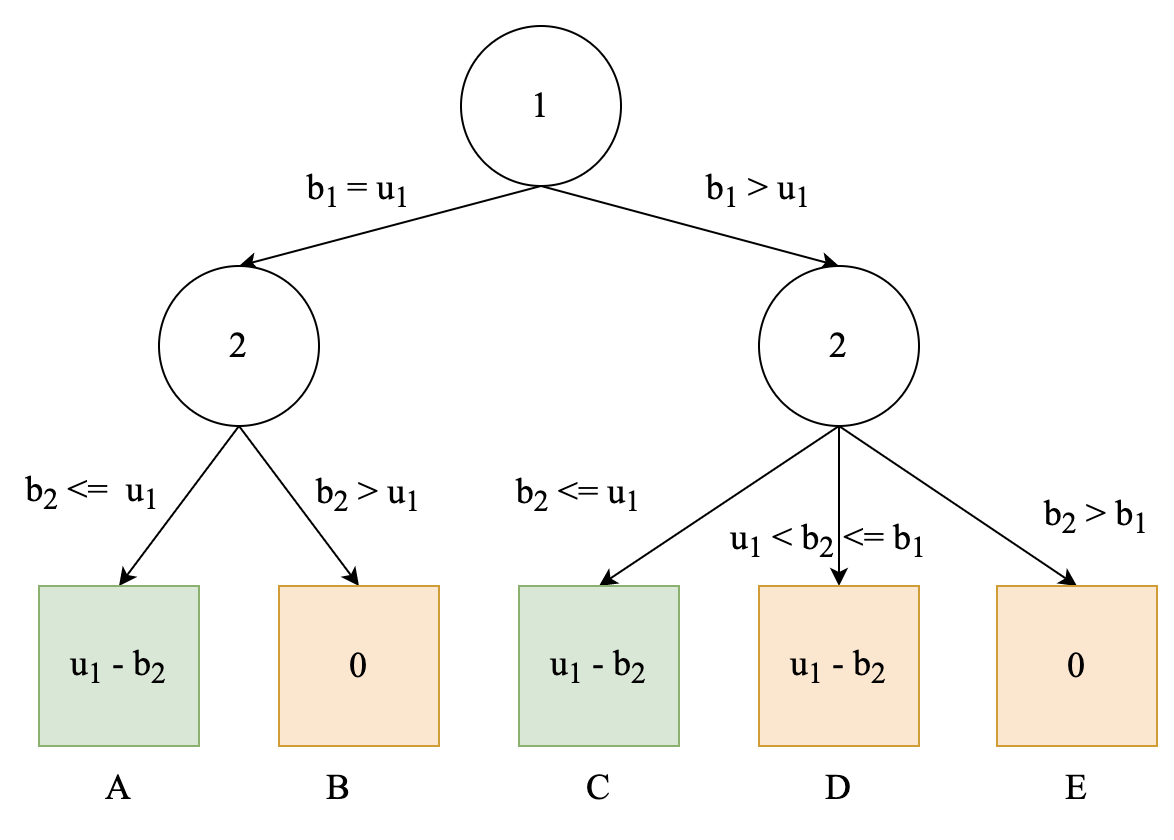
(a) Agent in a Second-Price Sealed Auction

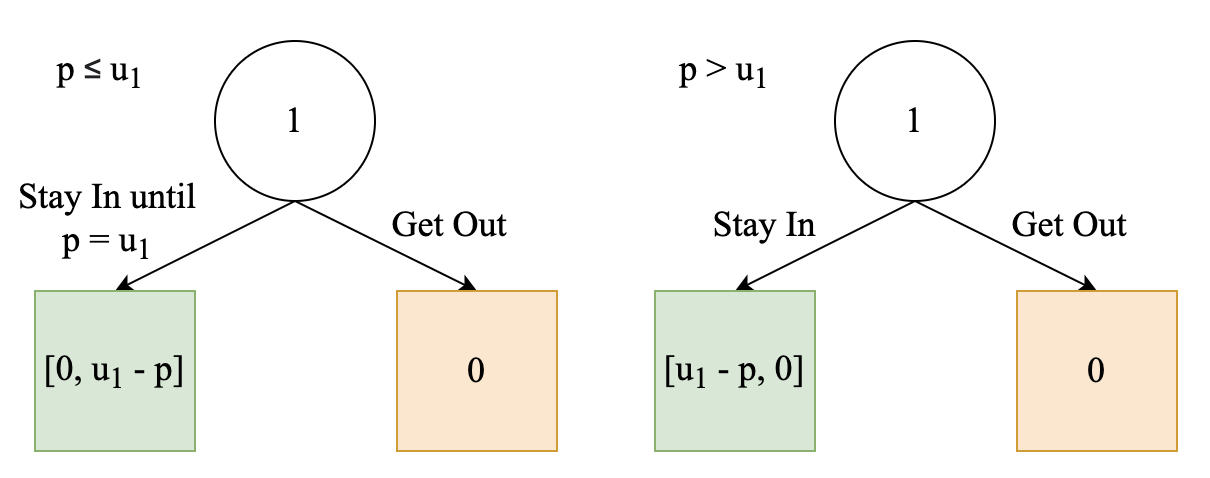
(b) Agent in an Ascending Clock Auction

Figure 3: SPSA vs. Ascending Clock Auction.

In the first scenario, getting out grants a utility of zero. Staying in until $p=u_{1}$ can grant utility no worse than 0 since the agent either loses (utility 0) or wins (utility $u_{1}-p\geq 0$). Therefore, the infinum of staying in (0) is weakly greater than the supremum of getting out (0).

In the second scenario, getting out grants a utility of zero. Staying in grants at most zero utility. Winning at this point will grant $u_{1}-p$ utility, which is always less than zero. Losing in a future round grants zero utility. Therefore, the supremum of deviating by staying in is zero, which is weakly dominated by getting out (utility 0). Therefore, ascending clock auctions are OSP.

Appendix C Missing Proofs

C.1 Proof of Proposition 3.4

Given that a voting rule $f$ reduces to a clocked election $CE$, we will show that for any arbitrary $\boldsymbol{\sigma}$ adding a clone to set of clones $K$ (where $|K|\geq 1$) in order to produce a voting profile $\boldsymbol{\sigma^{\prime\prime}}$ always results in:

1. $f(\boldsymbol{\sigma}^{\prime\prime})=f(\boldsymbol{\sigma})$ if $f(\boldsymbol{\sigma})\notin K$,

2. $f(\boldsymbol{\sigma}^{\prime\prime})\in K$ if $f(\boldsymbol{\sigma})\notin K$.

If true, we can extend this reasoning inductively to argue that the voting rule is independent of clones.

Say $F$ is the list that $CE$ would output on $\boldsymbol{\sigma}$ and $F^{\prime\prime}$ is the list that $CE$ would output on $\boldsymbol{\sigma}^{\prime\prime}$. Now, fix any $d\in K$, and let $F^{\prime}$ be the list that $CE$ would output on $\boldsymbol{\sigma}\setminus({K\setminus\{d\}})$ and $F^{\prime\prime\prime}$ the list that $CE$ would output on $\boldsymbol{\sigma^{\prime\prime}}\setminus({K\setminus\{d\}})$. First, notice that $F^{\prime}$ and $F^{\prime\prime\prime}$ are the same list, since by construction, $\boldsymbol{\sigma}\setminus({K\setminus\{d\}})$ is equivalent to $\boldsymbol{\sigma^{\prime\prime}}\setminus({K\setminus\{d\}})$.

We now consider the two cases presented above:

1. First, assume $f(\boldsymbol{\sigma})\notin K$, implying $(A\setminus F_{m-1})\cap K=\emptyset$. Suppose for contradiction that we have $f(\boldsymbol{\sigma})\neq f(\boldsymbol{\sigma^{\prime\prime}})$. Notice we have $\nexists g\in K$ such that $g\notin F_{m-1}$. Therefore, by Conditions $\boxed{4}$ and $\boxed{1}$, with $g^{*}$ being the clone with the largest index in $F_{m-1}$, $F_{m-1}\setminus(K\setminus\{g^{*}\})$ with $g^{*}$ replaced with $d$ must be equal to $F^{\prime}_{j}$ for some $j\in\{0,1,...,m-1\}$. Therefore, this $F^{\prime}_{j}$ must contain all of the candidates in $A\setminus(K\setminus\{d\})$ except $f(\boldsymbol{\sigma})$, implying $F^{\prime}_{j}$ is the final list of $F^{\prime}$. Similarly, consider $F^{\prime\prime}_{m}$. Since $f(\boldsymbol{\sigma})\in F^{\prime\prime}_{m}$ and $f(\boldsymbol{\sigma})\notin K$ by assumption, regardless of whether $F^{\prime\prime}_{m}$ fits to (a) or (b), Condition $\boxed{1}$ we must have $f(\boldsymbol{\sigma})\in F^{\prime\prime\prime}_{k}$ for some $k\in\{1,...,m\}$. However, then we have $f(\boldsymbol{\sigma})\notin F^{\prime}$ and $f(\boldsymbol{\sigma})\in F^{\prime\prime\prime}$, which creates a contradiction since $F^{\prime}=F^{\prime\prime\prime}$. Therefore, it must be that $f(\boldsymbol{\sigma})=f(\boldsymbol{\sigma^{\prime\prime}})$. More informally, if no member of the set of clones wins the original election, the addition of a clone has no effect on the winner of the clocked election.

2. Second, consider $f(\boldsymbol{\sigma})\in K$. We want to show that $f(\boldsymbol{\sigma}^{\prime\prime})\in K$. That is, if a member of the set of clones wins the original clocked election, in the perturbed clocked election, the winner is still a member of the set of clones. Suppose for contradiction, that this is not the case, that $f(\boldsymbol{\sigma})\in K$ but $f(\boldsymbol{\sigma^{\prime\prime}})\notin K$. By Condition $\boxed{1}$, since $\exists g\in K$ such that $g\notin F_{m-1}$, then there must exist some $F^{\prime}_{j}$ such that $F_{m-1}\setminus K=F^{\prime}_{j}$. $F^{\prime}_{j}$ therefore consists of an ordered list of $A\setminus(K\setminus\{f(\boldsymbol{\sigma})\})$, which has $m-|K|+1$ elements. In contrast, since $f(\boldsymbol{\sigma^{\prime\prime}})\notin K$, $\nexists g\in K$ such that $g\notin F^{\prime\prime}_{m}$. Therefore, $F^{\prime\prime}_{m}\setminus(K\setminus\{g^{*}\})$ (where $g^{*}$ is the last surviving candidate of $F^{\prime\prime}_{m}$) with $g^{*}$ replaced with $d$ must be equal to some $F^{\prime\prime\prime}_{k}$. Notice $|F^{\prime\prime\prime}_{k}|=|F^{\prime\prime}_{m}|-|K|+1=m-|K|+1=|F^{\prime}_{j}|$, implying $F^{\prime\prime\prime}_{k}=F^{\prime}_{j}$ since $F^{\prime\prime\prime}=F^{\prime}$. However, we have $f(\boldsymbol{\sigma}^{\prime\prime})\in F^{\prime}_{j}$ since $f(\boldsymbol{\sigma}^{\prime\prime})\notin K$ and $A\setminus K\subset F^{\prime}_{j}$, but $f(\boldsymbol{\sigma}^{\prime\prime})\notin F^{\prime\prime\prime}_{k}$ by Condition $\boxed{4}$, which is a contradiction. Hence, we must have $f(\boldsymbol{\sigma}^{\prime\prime})\in K$. More informally, a member of the set of clones wins the original election, the addition of a clone results in a candidate from the same set of clones to win the election.

∎

C.2 Proof of Proposition 3.5

Given an arbitrary IoC election mechanism $f$, it is always possible to create a clocked election that fulfills Conditions $\boxed{1}$, $\boxed{3}$, and $\boxed{4}$. Given voting profile $\boldsymbol{\sigma}$, such a mechanism would simply run $f$ on $\boldsymbol{\sigma}$ to produce $f(\boldsymbol{\sigma})$. Then, the mechanism would designate $A\setminus F_{m-1}$ to be $f(\boldsymbol{\sigma})$ and subsequently assign clones of $f(\boldsymbol{\sigma})$ to $F_{m-1}\setminus F_{m-2}$ (i.e., the $(m-1)$-th position of $F$), $F_{m-2}\setminus F_{m-3}$ (i.e., the $(m-2)$-th position in $F$), and so on. Then, the mechanism can order the remaining non-clone candidates (i.e., one candidate from each set of clones) using any deterministic ordering function that satisfies neutrality and independence of clones. After re-ordering the non-clone candidates, the mechanism inserts each clone candidate such that all candidates from a set of clones are adjacent and orders the clones amongst themselves using a deterministic ordering function. This continues until a final complete ordering is achieved. Since the winning candidate is always inserted at the end of the list, this mechanism satisfies Condition $\boxed{4}$. Since we only use deterministic ordering functions that satisfy neutrality, Condition $\boxed{3}$ is fulfilled. Furthermore, we can show that this mechanism satisfies both cases of Condition $\boxed{1}$. Suppose that for any set of clones $K$ and any $d\in K$, $F^{\prime}$ is the list of eliminated candidates when the clocked election designed above is run on $\boldsymbol{\sigma}\setminus(K\setminus\{d\})$.

1. We want to show that for any set of clones $K$, for all $F_{i}$ such that $\exists g\in K$ such that $g\notin F_{i}$, there must exist a $F^{\prime}_{j}$ such that $F_{i}\setminus K=F^{\prime}_{j}$. Since clone insertion occurs after the initial deterministic ordering phase, changing the size of any set of clones does not change the relative ordering of non-clone candidates. Furthermore, since inter-clone ordering is unaffected, the ordered list is also unaffected. In particular, since $f$ is independent of clones, the new winner should also be a member of the same set of clones as $f(\boldsymbol{\sigma})$, even if $f(\boldsymbol{\sigma})$ was removed. This ensures that the set of clones that appear last in $F$ stay the same, hence ensuring the clocked election fulfills this condition.

2. We want show that for all other $F_{i}$, let $g^{*}\in K$ be the clone with the largest index in $F_{i}$. We want to show that $F_{i}\setminus(K\setminus\{g^{*}\})$ with $g^{*}$ replaced with $d$ is equal to $F^{\prime}_{j}$ for some $j\in\{0,1,\ldots,m-1\}$. Note that the order of all the candidates in $A\setminus K$ is the same for $F$ and $F^{\prime}$ by the same justification as $(a)$. Lastly, since the candidates in $K$ appear together in the ranking in $F$, removing all but the longest surviving candidate (i.e., $g^{*}$) from $F$ will simply result in $g^{*}$ appearing alone in where the set of clones used to be (as, once again, the order of the set of clones is preserved). Similarly, in $F^{\prime}$, since the order of the sets of clones in the same as it appears in $F$, the place that was taken by $K$ is now solely taken by $d$. This shows that $F\setminus(K\setminus\{g^{*}\})$ where $g^{*}$ is replaced with $d$ is the same as $F^{\prime}$, hence fulfilling the condition for all $F_{i}$ that appears after the index of $g^{*}$ in $F$, as desired.

∎

C.3 Proof of Theorem 4.2

We want to show that the $CE_{STV}$ Protocol, as defined in Definition 4.1, fulfills the four conditions of a Clocked Election, given in Definition 3.2.

Condition 1: Given a preference profile $\boldsymbol{\sigma}$, for any set of clones $K\subset A$ and any $d\in K$, let $F^{\prime}$ be the list that $CE_{STV}$ would output on $\boldsymbol{\sigma}^{\prime}=\boldsymbol{\sigma}\setminus(K\setminus\{d\})$. Note that $F=F^{\prime}$ for $|K|=1$, so Condition 1 is trivially satisfied. Consider $|K|>1$. We would like to do a proof by induction on the step $i$ that each $F_{i}$ satisfies one of (a) or (b) listed under Condition 1.

Base case: Let $i=1$. Note that $|F_{1}|=1$ and $|K|>2$, so $F_{1}$ needs to satisfy (a). First consider the case in which $F_{1}=\{g\}$ for some $g\in K$. Then $F_{1}\setminus K=\emptyset=F^{\prime}_{0}$, so (a) is indeed satisfied. Now, consider the case where $F_{1}=\{a\}$ for some $a\notin K$. This implies $a$ was the candidate that appeared the least on the top row of $\boldsymbol{\sigma}$. Notice that by definition of clones the top row of $\boldsymbol{\sigma}^{\prime}$ is identical to that of $\boldsymbol{\sigma}$ except each $g\in K\setminus\{d\}$ is replaced with $d$ (since the clones on the top row transfer their votes to $d$ once all the other clones are removed from $\boldsymbol{\sigma}$). So the number of plurality votes for each remaining candidate in $\boldsymbol{\sigma}^{\prime}$ is the same as their plurality vote in $\boldsymbol{\sigma}$, except for $d$, whose plurality vote in $\boldsymbol{\sigma}^{\prime}$ is greater or equal to its plurality vote in $\boldsymbol{\sigma}$. Since no candidate had their plurality vote decrease, $a$ is still the candidate with the least amount of plurality votes in $\boldsymbol{\sigma}^{\prime}$, implying $F^{\prime}_{1}=\{a\}$ and hence $F_{1}=F^{\prime}_{1}$, as desired.
Inductive case: Assume $F_{i}$ satisfies Condition 1, implying it either satisfies (a) or (b). We want to show that $F_{i+1}$ satisfies Condition 1 in either of these cases.

• If $F_{i}$ satisfies (a), this implies $\exists g\in K$ such that $g\notin F_{i}$ and that $F_{i}\setminus K=F^{\prime}_{j}$ for some $j\in\{0,1,...,m-1\}$ (where $F^{\prime}_{0}$ is defined as the empty set $\emptyset$). First consider the case $F_{i+1}=F_{i}\cup\{g\}$ and $K\subset F_{i+1}$, so the last clone is eliminated. This implies that $A\setminus F_{i}$ includes a single clone $g$. Similarly, $F^{\prime}_{j}=F_{i}\setminus K$, which implies $A\setminus F_{i}$ is the same as $A^{\prime}\setminus F^{\prime}_{j}$ (where $A^{\prime}=A\setminus(K\setminus\{d\}))$ except with $g$ replaced by $d$ in the latter. Hence, $\boldsymbol{\sigma}_{i}$ and $\boldsymbol{\sigma}^{\prime}_{j}$ (the preference profile of remaining candidates after removing the candidates $F_{i}$ or $F^{\prime}_{j}$, respectively) is identical except for $g$ is replaced by $d$ in $\boldsymbol{\sigma}^{\prime}_{j}$. Since $g$ has the least plurality votes in $\boldsymbol{\sigma}_{i}$, then $d$ must have the least plurality votes in $\boldsymbol{\sigma}^{\prime}_{j}$, implying $F^{\prime}_{j+1}=F^{\prime}_{j}\cup\{d\}$. Since $g$ is the clone with the largest index in $F_{i+1}$, and since $F_{i}\setminus K=F^{\prime}_{j}$, then $F_{i+1}\setminus(K\setminus\{g\})=(F_{i}\setminus K)\cup\{g\}=F^{\prime}_{j}\cup\{g\}$ where we replace $g$ with $d$ is $F^{\prime}_{j}\cup\{d\}=F^{\prime}_{j+1}$, showing that $F_{i+1}$ satisfies (b). Second, consider the case in which $F_{i+1}=F_{i}\cup\{g\}$ and $\exists g^{\prime}\in K$ such that $g^{\prime}\in A\setminus F_{i+1}$, so there are still clones remaining in the contest. In that case, $F_{i+1}\setminus K=F_{i}\cup\{g\}\setminus K=F_{i}\setminus K=F^{\prime}_{j}$ by assumption, so $F_{i+1}$ satisfies (a). Lastly, consider the case $F_{i+1}=F_{i}\cup\{a\}$ for some $a\notin K$. This implies $a$ was the candidate that appeared the least on the top non-NULL entries of each column $\boldsymbol{\sigma}_{i}$. Notice that by definition of clones the top row of $\boldsymbol{\sigma}^{\prime}_{j}$ is identical to that of $\boldsymbol{\sigma}_{i}$ except each $g\in K\setminus\{d\}$ is replaced with $d$ (since the clones on the top row transfer their votes to $d$ once all the other clones are removed from $\boldsymbol{\sigma}_{i}$). This follows from the fact that all the non-clone candidates eliminated to produce $\boldsymbol{\sigma}_{i}$ are identical to the non-clone candidates eliminated to produce $\boldsymbol{\sigma}^{\prime}_{j}$, and there is still at least one clone remaining by assumption. So the number of plurality votes for each remaining candidate in $\boldsymbol{\sigma}^{\prime}_{j}$ is the same as their plurality vote in $\boldsymbol{\sigma}_{i}$, except for $d$, whose plurality vote in $\boldsymbol{\sigma}^{\prime}_{j}$ is greater or equal to its plurality vote in $\boldsymbol{\sigma}_{i}$ (this is true even if $d\in F_{i}$, in which case it has it has zero plurality votes in $\boldsymbol{\sigma}_{i}$). Since no candidate had their plurality vote decrease, $a$ is still the candidate with the least amount of plurality votes in $\boldsymbol{\sigma}^{\prime}_{j}$, implying $F^{\prime}_{j+1}=F^{\prime}_{j}\cup\{a\}=F_{i}\cup\{a\}\setminus K=F_{i+1}\setminus K$ and hence $F_{i+1}$ satisfies (a).

• If $F_{i}$ satisfies (b), this implies $K\subset F_{i}$ and if given that $g^{*}$ is the clone with the highest index in $F_{i}$, then $F_{i}\setminus(K\setminus g^{*})$ with $g^{*}$ replaced with $d$ is equal to $F^{\prime}_{j}$ for some $j\in\{0,...,m-1\}$. Since $K\subset F_{i}$ and $d\in F^{\prime}_{j}$, all the clones are eliminated in both cases, implying $\boldsymbol{\sigma}_{i}$ is identical to $\boldsymbol{\sigma}^{\prime}_{j}$ ignoring NULL values. Hence, the next candidate with the least plurality votes should be the same in both cases (say $a$). Since $F^{\prime}_{j}$ is equal to $F_{i}\setminus(K\setminus g^{*})$ with $g^{*}$ replaced with $d$ , then $F^{\prime}_{j+1}=F^{\prime}_{j}\cup\{a\}$ is equal to $F_{i}\cup\{a\}\setminus(K\setminus g^{*})=F_{i+1}\setminus(K\setminus g^{*})$ with $g^{*}$ replaced with $d$, showing that $F_{i+1}$ satisfies (b).

Hence, in either case, $F_{j+1}$ satisfies Condition 1, completing the inductive case.

Condition 2: This condition follows from the fact that when $CE_{STV}$ produces $F_{i}$ by looking at at most the top $i$ entries of each column. Hence, the bounded agent is clueless about how the last $m-i$ rows of $\boldsymbol{\sigma}$ are distributed, implying that it cannot predict the remaining order in which the candidates will be eliminated (as it will not know which candidates will receive the transfered votes of the eliminated candidates in future steps). It is worth noting that if more than half of the plurality votes went to the same candidate at step $i$, an agent given this information could deduct that this candidate will be the final winner and hence deduct that the other candidates will be eliminated. However, knowing that a candidate received more than half of the plurality votes would involve dividing number of plurality voter received by the candidate by the total number of votes, an operation that is never conducted by $CE_{STV}$, which instead only calculates the candidate with the least plurality votes on each round through comparisons. Since the number of total votes is $O(n)$, dividing the plurality votes received by a candidate by the total number of votes cannot be calculated in constant time. Thus, as specified in Definition 3.1, the bounded agent is not capable of performing such a division, and hence can never deduct that a candidate is the winner until all other candidates are eliminated.

Condition 3: The neutrality of this method follows from the neutrality of STV, and more specifically from the fact that at each step, the candidate that is eliminated is only dependent on the remaining plurality votes, so if we permuted the labels of the candidates, the order in which they are eliminated would also get permuted in the same way.

Condition 4: $A\setminus F_{m-1}$ does indeed give us the STV winner, which follows from the fact that $CE_{STV}$ follows the rules of STV at each step by eliminating the voter with the least plurality votes and transferring the votes of each voter that voted for this candidate to their next choice. ∎

C.4 Proof of Theorem 4.5

We want to show that the $CE_{RP}$ Protocol, as defined in Definition 4.4, fulfills the four conditions of a Clocked Election, given in Definition 3.2.

Condition 1: For any set of clones $K\subset A$ and any $d\in K$, say $F^{\prime}$ is the list that $CE_{STV}$ would output on $\boldsymbol{\sigma}^{\prime}=\boldsymbol{\sigma}\setminus(K\setminus\{d\})$. Note that $F=F^{\prime}$ for $|K|=1$, so Condition 1 is trivially satisfied. Consider $|K|>1$. Say $M$ and $M^{\prime}$ are the majority matrices produced by the protocol on input $\boldsymbol{\sigma}$ and $\boldsymbol{\sigma}^{\prime}$, respectively. Similarly, say that $O$ and $O^{\prime}$ are ordered lists of edges $(a,b)$ in decreasing order of $M_{a,b}$ and $M^{\prime}_{a,b}$, respectively (which is the order in which the protocol will consider these edges). Notice that $\forall a,b\in A\setminus(K\setminus\{d\})$, we have $M_{a,b}=M^{\prime}_{a,b}$, so the order in which these edges appear in both $O$ and $O^{\prime}$ are the same. The only additional edges contained in $O$ and not in $O^{\prime}$ are the ones involving clones other than $d$. It follows from the definition of clones that for any $g\in K$ and any $a\in A\setminus K$, we have $M_{g,a}=M^{\prime}_{d,a}$ and $M_{a,g}=M^{\prime}_{a,d}$. Hence, in $O$, all such $M_{g,a}$ is tied with $M_{d,a}$ and all such $M_{a,g}$ is tied with $M_{a,d}$. In addition, $O$ also contains edges $(g,g^{\prime})$ for any $g,g^{\prime}\in K$, which $O^{\prime}$ do not contain. Note that such edges could be located anywhere in $O$, since we have no information on $M_{g,g^{\prime}}$. Say $G(V,E)$ and $G^{\prime}(V,E^{\prime})$ are the final graphs produced by running the protocol on majority matrices produced by the protocol on input $\boldsymbol{\sigma}$ and $\boldsymbol{\sigma}^{\prime}$, respectively. We would like to show that any $(a,b)\in O\cap O^{\prime}$ is in $E$ if and only if it is in $E^{\prime}$ for $a,b\neq d$, and an edge $(d,b)$ (or similarly $(a,d)$) in $E$ if and only if it and all other $(g,b)$ (or similarly $(a,g)$) for $g\in K$ is in $E^{\prime}$. We do this by induction on the order in which these edges appear in $O^{\prime}$:

Base case: First element in $O^{\prime}$. Note that the first element in $O^{\prime}$ (say $(a,b)$) will always be added to the graph by the $CE_{RP}(\boldsymbol{\sigma}^{\prime})$, since it is the first edge and cannot create a cycle. Since elements of $O^{\prime}$ appear in the same order in $O$, when $CE_{RP}(\boldsymbol{\sigma})$ considers $(a,b)$, the edges already added to $E$ could only be of the form $(g,g^{\prime})$ for $g,g^{\prime};\in K$, $(a,g)$ for $g\in K$ (if $b=d$) and $(g,b)$ for $g\in K$ (if $a=d$). Any cycle containing $(a,b)$ would need an edge $(g,a)$ and an edge $(b,g^{\prime})$ in it with $g,g^{\prime}\in K$. Since we cannot have $a=b=d$, at most only one of $a$ or $b$ is in $K$, it is impossible for the protocol to have already considered $(g,a)$ and $(b,g^{\prime})$, implying that $(a,b)$ gets added to the graph by $CE_{RP}(\boldsymbol{\sigma})$. If we have $a=d$ (or similarly $b=d$) then all $(g,b)$ (or similarly $(a,g)$) for $g\in K$ would appear tied in $O$ with $(a,b)$. Since only one of these vertices is a clone, the same arguement about the impossibility of cycles apply, so all such $(g,b)$ (or similarly $(a,g)$) also gets added to $G$, as desired.

Inductive case: Say the first $i$ elements in $O^{\prime}$ satisfy the condition, and show that this holds true for the $i+1$th element. Note that since the element of $O^{\prime}$ appear in the same order in $O$, the first $i$ elements in $O^{\prime}$ have already been considered by $CE_{RP}(\boldsymbol{\sigma})$ once the $i+1$th element of $O^{\prime}$ (say $(a,b)$) is considered. Say $(a,b)\notin G^{\prime}$. This implies that $(a,b)$ form a cycle with the edges in the first $i$ elements of $O^{\prime}$ that were added to $G^{\prime}$. But these edges are also added to the $G$ by the inductive hypothesis, so the same cycle would form if $(a,b)$ was added to $G$. Hence, $(a,b)$ does not get added to $G$ if it is not added to $G^{\prime}$.

Conversely, say $(a,b)$ was added to $G^{\prime}$, implying it does not form a cycle with the edges in the first $i$ elements of $O^{\prime}$ that were added to $G^{\prime}$. The only additional edges that might have already added to $G$ once $CE_{RP}(\boldsymbol{\sigma})$ considers $(a,b)$ are the ones involving clones. Thus, any cycle that $(a,b)$ might cause in $G$ must involve clones. If this cycle contained only a single clone, say $g$, the same cycle would have formed in $G^{\prime}$ with $g$ replaced with $d$ (since all the edges weights of $d$ are the same as those of $g$, as shown above, and since an edge containing $g$ is in the $G$ iff the analogous edge containing $d$ is in the $G^{\prime}$ and $G$, by the inductive hypothesis), which is a contradiction. If the cycle contained multiple clones, on the other hand, say $g$ is the first clone that appears in the cycle via edge $(x,g)$ and $g^{\prime}$ is the last (via edge $(g^{\prime},y)$) then we could replace these edges, along with the edges that come in between, with $(x,d)$ and $(d,y)$ (which need to be in the graph by the inductive hypothesis) and still form the cycle, which is a contradiction. Hence, $(a,b)$ does not form a cycle. The argument for how edges containing $d$ are added to $G$ iff all analogous edges containing any $g\in G$ is analogous to that in the base case: any cycle that would form by one would form by the other, since all the edges that have been added so far fulfilled this condition by the inductive hypothesis. This concludes the inductive case.

Hence, an edge in $O^{\prime}$ appears in $G$ iff it appears in $G^{\prime}$, and these edges get added in the same order as the elements in $O^{\prime}$ appear in the same order in $O$. Hence, if all the candidates $b\in F^{\prime}$ that were eliminated by an edge (say $(a,b)$) in $G^{\prime}$ were eliminated by the same edge in $G$, the ordering of these candidates would be the same in both $F$ and $F^{\prime}$. Note that by the induction above, the only other way $b$ could have been eliminated by a different edge by $CE_{RP}(\boldsymbol{\sigma})$ is if $a=d$ and $b$ gets eliminated by another $(g,b)$. However, since $(g,b)$ has the same weight as $(d,b)$, this would not disrupt the order in which $b$ is eliminated with respect to the other candidates. Hence, all the none-cloned candidates appear in the same order in $F$ and $F^{\prime}$, fulfilling (a) of Condition 1.

To see that (b) is also satisfied whenever relevant, assume that the winner is not among the clones (otherwise (b) would be vacuously satisfied). Notice that the clones in $K$ can be eliminated by edges of form $(g,g^{\prime})$ for $g,g^{\prime}\in K$ in any arbitrary step (since these edges can appear anywhere in $O$) but the last clone $g^{*}$ must always be eliminated by an edge $(a,g^{*})$ for $a\notin K$ (since if all clones were eliminated by edges of form $(g,g^{\prime})$, then we would have a cycle, which is a contradiction). The analogous edge $(a,d)$ gets added to $G^{\prime}$ in the same order by the induction above, so $g^{*}$ gets eliminated by $CE_{RP}(\boldsymbol{\sigma})$ by an analogous edge that eliminates $d$ by $CE_{RP}(\boldsymbol{\sigma}^{\prime})$ showing that $g^{*}$ replaces $d$ when going from $F^{\prime}$ to $F$, hence satisfying (b). Thus, the lists $F$ and $F^{\prime}$ do indeed satisfy Condition 1.

Condition 2: This follows from the definition of a bounded agent, who is incapable of making comparisons of numbers or run max/min queries on the majority matrix, as such strength comparisons and min/max operations cannot be calculated in constant time considering there are $O(m^{2})$ numbers to be compared, each of size $O(n)$. Hence, after step $i$ (when $F_{i}$ is computed, $M^{(i)}$ is the current majority matrix and $G_{i}$ is the current graph), the bounded agent cannot query $M^{(i)}$ to get the next largest non-NULL entry, hence there is no way for it to know which candidates will be eliminated next. To see this more formally, for any candidate $a\notin F_{i}$ the next $m-1$ largest weight edges in $M^{(i)}$ could be of form $(a,b)$ for each $b\in A\setminus\{a\}$, and all of these would be added to $G_{i}$ since $a$ currently has no incoming edges (as evidenced by $a\notin F_{i}$) so none of these edges could form a cycle. Adding all of these edges to $G_{i}$ would ensure that $a$ is the final winner, as no edge pointing to it can be added any longer without forming a cycle. Since this is true of all $a\notin F_{i}$, and since the bounded agent cannot distinguish between these cases without querying $M^{(i)}$, it is not possible for it to predict with certainty that any $a\notin F_{i}$ will be eliminated in the next $m-1-i$ rounds.

Condition 3: The neutrality of this method follows from the neutrality of Ranked Pairs, and more specifically from the fact that at each step, the edges that are added (and hence the candidates that are eliminated) is only dependent on the majority matrix, so if we permuted the labels of the candidates (and hence the rows/columns of $M)$, the order in which they are eliminated would also get permuted in the same way.

Condition 4: $A\setminus F_{m-1}$ does indeed give us the Ranked Pairs winner, which follows from the fact that $CE_{RP}$ follows the rules of Ranked Pairs at each step by forming a cycle from the edges with highest majority scores without forming cycles. ∎

C.5 Proof of Theorem 4.7

Based on Definition 3.3, in order to prove Theorem 4.7, we must show that the Schulze Method cannot be reduced to a clocked election. Assume for the sake of contradiction that there exits a protocol $CE_{S}$ that is a Clocked Election for the Schulze Method, i.e. it fulfills the four conditions given in Definition 3.2, which we will denote as Conditions $\boxed{1}$, $\boxed{2}$, $\boxed{3}$, and $\boxed{4}$ for clarity. We will also denote the strength matrix (as introduced in Section 2.2) by $S$.

Note that by condition $\boxed{4}$, run on any preference profile $\boldsymbol{\sigma}$ with candidates $A$ and voters $N$, the list $F$ that $CE_{S}$ outputs contains all the candidates except for the winner of the Schulze Method applied to the profile. The winner corresponds to $f_{S}(\boldsymbol{\sigma})$. Notice that for any $a\in A$, we have $f_{S}(\boldsymbol{\sigma})=a\Leftrightarrow S[a,b]>S[b,a]\,\forall b\in A\setminus\{a\}$). As such, for any $b$ that gets added to $F_{i}$ on step $i$, since $b\neq f_{S}(\boldsymbol{\sigma})$, the protocol must first ensure that $\exists c\in A\setminus\{b\}$ such that $S[c,b]>S[b,c]$, which it cannot do without without computing and comparing $S[c,b]$ and $S[b,c]$ at least for one $c\in A\setminus\{b\}$. Note that at any step $i<m-1$ (i.e., after the production of $F_{i}$) if the protocol has made the comparison $S[a,b]>S[b,a]$ for some $a,b\in A$. But if $b\notin F_{i}$, then the bounded agent reading all the logs up to step $i$ (which the bounded agent is allowed to do by Definition 3.1) would be capable of deducting that $b$ is not the Schulze winner, and hence determine in constant time that $b\in F_{m-1}$. Moreover, a constant time algorithm that is programmed to output a candidate $b\in A\setminus F_{i}$ as soon as it sees the comparison $S[a,b]>S[b,a]$ in the logs of the $CE_{S}$ up to $F_{i}$ (say $\mathcal{L}$) would succeed with probability 1 over all possible $\boldsymbol{\sigma}$ that lead to $\mathcal{L}$ (as $b\in F_{m-1}$ for all such $\boldsymbol{\sigma}$), and hence violate the assumption that $CE_{S}$ satisfies Condition $\boxed{2}$.

The implications of this contradiction are twofold: first, this implies that the protocol must decide on a order of candidates (say $\pi:\{1,...,m\}\rightarrow A$, injective) in which it will perform such comparisons (which should be an order that cannot be based on the final ranking of the candidates, as there is no way for the protocol to know the ranking a priory without computing it, which would again violate Condition $\boxed{2}$), such that at step $i$ it compares $\pi(i)$ with all $\pi(j)$ such that $j<i$ (which must produce exactly one new eliminated candidate by transitivity). Secondly, as shown above, we cannot have that the comparison $S[a,b]>S[b,a]$ has been made before producing $F_{i}$ but still have $b\notin F_{i}$, which implies that the protocol can compare exactly one new candidate between outputting $F_{i}$ and $F_{i+1}$ for all $i\in[m-1]$. In other words, the protocol must compare $\pi(i)$ with $\pi(j)$ such that $j<i$ exactly between outputting $F_{i-2}$ and $F_{i-1}$ (since the first eliminated candidate is placed in $F_{1}$ and results from comparing $\pi(2)$ with $\pi(1)$).

We now show that this $\pi$ must be a deterministic function of the preference profile, independent of any arbitrary orderings of the candidates. Suppose instead that the protocol could determine $\pi$ arbitrarily (i.e., using an arbitrary ordering of the candidates in $A$) and consider a 4-candidate election that consists of a preference profile $\boldsymbol{\sigma}_{0}$ with $A=\{a,b,c,d\}$ that has $a>b>c>d$ as its final Schulze ranking. Note that we know by transitivity that such a ranking exists for all possible $\boldsymbol{\sigma}$ with four candidates. Say that $\pi_{0}$ is the order in which $CE_{S}$ computes candidates when given $\boldsymbol{\sigma}_{0}$ as an input. Consider the permutation $\tau_{1}:A\rightarrow A$ that has $\tau_{1}(\pi_{0}(1))=b$, $\tau_{1}(\pi_{0}(2))=c$, $\tau_{1}(\pi_{0}(3))=d$, and $\tau_{1}(\pi_{0}(4))=a$. Let $\boldsymbol{\sigma}_{1}$ be the preference profile constructed by applying $\tau_{1}$ to $\boldsymbol{\sigma}_{0}$. Since $CE_{S}$ produces $\pi_{0}$ using an arbitrary ordering of candidates (i.e., independent of the actual votes), then given $\boldsymbol{\sigma}_{1}$ as an input, it must compare the candidates with ordering $\pi_{1}=\{b,c,d,a\}$. Then comparison in the first step will give $b>c$ ($F_{1}=\{c\}$), the comparisons in the second step will give partial ranking $b>c>d$ ($F_{2}=\{c,d\}$), and the comparisons in the third step will give final ranking $a>b>c>d$ ($F_{3}=\{c,d,b\}$). Now consider a second permutation $\tau_{2}$ that maps $\tau_{2}(a)=c$, $\tau_{2}(b)=a$, $\tau_{2}(c)=d$, and $\tau_{2}(d)=b$ and say $\boldsymbol{\sigma}_{2}$ is the preference profile constructed by applying $\tau_{2}$ to $\boldsymbol{\sigma}_{1}$. Since $CE_{S}$ produces an arbitrary ordering of candidates (independent of actual votes), and since it produced order $\pi_{1}=\{b,c,d,a\}$ when given $\boldsymbol{\sigma}_{1}$ as an input, it must produce order $\pi_{2}=\{a,d,b,c\}$ when given $\boldsymbol{\sigma}_{2}$ as an input. Performing the comparisons in this order, the comparison in step 1 will give $a>d$ $(F^{\prime}_{1}=\{d\})$, the comparisons in step 2 will give $a>b>d$ $(F^{\prime}_{2}=\{d,b\})$, and the comparisons in step 3 will give $a>b>c>d$ $(F^{\prime}_{3}=\{d,b,c\})$. So going from $\boldsymbol{\sigma}_{1}$ to $\boldsymbol{\sigma}_{2}$, the list that $CE_{S}$ outputs went from $F=\{c,d,b\}$ to $F^{\prime}=\{d,b,c\}$, which does not correspond to the permutation $\tau_{2}$ we performed on $\boldsymbol{\sigma}_{1}$ to produce $\boldsymbol{\sigma}_{2}$, which shows that any protocol that chooses the order in which the strength of the candidates are compared arbitrarily violates the assumption that $CE_{S}$ satisfies Condition $\boxed{3}$. Thus, it must choose the order of comparisons non-arbitrarily. The same cyclic argument can be applied to elections on $\mathit{n}$ candidates. Thus, we know that $CE_{S}$ must implement some function $h$ that produces the order in which the strengths of the candidates are compared and is independent of any arbitrary ordering of the candidates. Since the only source of non-arbitrariness in the Schulze method is the pairwise comparison matrix $P$ (as the strength matrix $S$ and hence the winner is entirely determined by this matrix), this implies that $h$ can be represented as a deterministic function takes $P$ as an input and outputs an order of candidates $\pi$, such that $CE_{S}$ performs the pairwise comparisons of strengths in this order.

The rest of the proof uses a new definition we now introduce:

Definition C.1 (Pseudo-clones).

Two candidates $a,b\in A$ are pseudo-clones with respect to the preference profile $\boldsymbol{\sigma}$ if:

1. $\forall c\in A\setminus\{a,b\}$, $P[a,c]=P[b,c]$ and $P[c,a]=P[b,c]$, where $P$ is the pairwise comparison matrix of $\boldsymbol{\sigma}$.

2. There does not exists a set of clones $K$ such that $a,b\in K$. As such, $a$ and $b$ are not clones.

The construction of preference profiles that contain pseudo-clones is indeed possible. One such example is provided below, along with corresponding pairwise comparison matrix:

Voter	Voter	Voter	Voter	Voter	Voter	Voter
1	2	3	4	5	6	7
a	b	c	a	b	b	c
b	a	a	c	c	a	b
d	c	b	b	a	d	a
c	d	d	d	d	c	d

$\Rightarrow$   $P$ a b c d a 0 3 4 7 b 4 0 4 7 c 3 3 0 5 d 0 0 2 0

As it can be seen from $P$, we indeed have that the candidates $a$ and $b$ have matching pairwise comparisons with the remaining candidates $(c$ and $d)$. However, $\{a,b\}$ is not a set of clones, since voters 4 and 5 rank $c$ between them. Similarly, $\{a,b,c\}$ is not a set of clones due to voters 1 and 6. Hence, $a$ and $b$ do not appear together in a set of clones, meaning that they are indeed pseudo-clones. However, the key point about the definition of pseudo-clones is that, even though $a$ and $b$ are not clones, this fact cannot be deduced from the pairwise comparison matrix $P$. That is, one cannot distinguish from $P$ alone whether $a$ and $b$ are clones or pseudoclones.

More generally, using the same setup, we can create any voting profile where $a,b$ are pseudo-clones such that the pairwise comparison matrix is:

$P$	a	b	c	d	e	…
a	0	$r$	$x$	$y$	$z$	$\ldots$
b	$n-r$	0	$x$	$y$	$z$	$\ldots$
c	$n-x$		0			$\ldots$
d	$n-y$			0		$\ldots$
e	$n-z$				0	…
$\vdots$	$\vdots$	$\vdots$	$\vdots$	$\vdots$	$\vdots$	$\ddots$

where $n$ is the number of voters. Notice that we can create this profile for all $x,y,z,...\in\{0,1,...,n\}$ and all $r\in\{1,...,n-1\}$. Similarly, the empty cells in the $P$ above can be filled with any $i\in\{0,\ldots,n\}$.

We now combine the notions of pseudo-clones and clones to complete the proof. Consider a preference profile $\boldsymbol{\sigma}$ for voters $N$ and candidates $A$ in which $a,b\in A$ are pseudo-clones, with $P[a,b]=r$ and $P[b,a]=n-r$ where $n=|N|$ and $P_{\boldsymbol{\sigma}}$ is the associated pairwise comparison matrix. WLOG, say $r\geq\frac{n}{2}$. Note that in a graphical representation of $P_{\boldsymbol{\sigma}}$, the edge $P_{\boldsymbol{\sigma}}[a,b]$ would appear as shown in Figure 4.

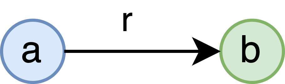
Figure 4: As a part of $P_{\boldsymbol{\sigma}}$.

Other than this edge (and the implied opposite edge corresponding to $P_{\boldsymbol{\sigma}}[b,a]=n-r$), by definition of pseudo-clones, all of the incoming and outgoing edges of $a$ and $b$ are the same. Now consider a new preference profile $\boldsymbol{\sigma}_{a}$, produced from by cloning $a$ in $\boldsymbol{\sigma}$. Say $a^{*}$ is the added clone. By definition of clones, we need to have $P[a^{*},b]=r$. The key idea is that as we go from $\boldsymbol{\sigma}$ to $\boldsymbol{\sigma}_{a}$ (and hence $P_{\boldsymbol{\sigma}}$ to $P_{\boldsymbol{\sigma_{a}}}$) we have the flexibility of arbitrarily choosing $P_{\boldsymbol{\sigma}_{a}}[a,a^{*}]$, since the only restriction is that $a$ and $a^{*}$ should appear consecutively in every voter’s ranking. Say we choose $P_{\boldsymbol{\sigma}_{a}}[a,a^{*}]=r$, in which case the partial graphical representation of $P_{\boldsymbol{\sigma}_{a}}$ would appear as shown in Figure 5(a). Note that the remaining incoming and outgoing edges from these three nodes (edges that are not shown in the figure) are identical to one another due to the definitions of clones and pseudo-clones.

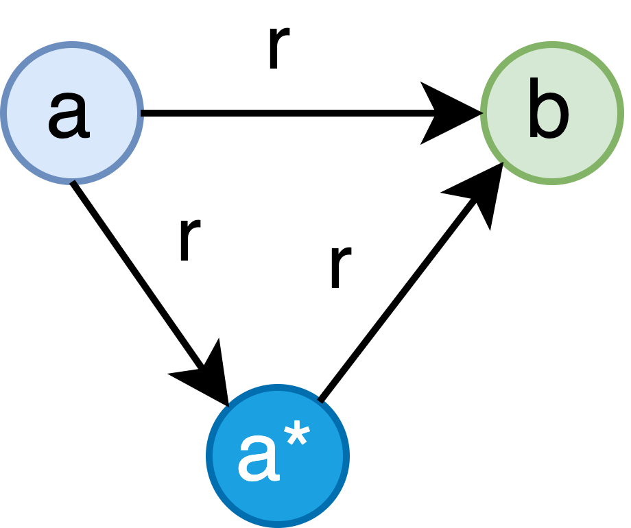
(a) As a part of $P_{\boldsymbol{\sigma}_{a}}$.

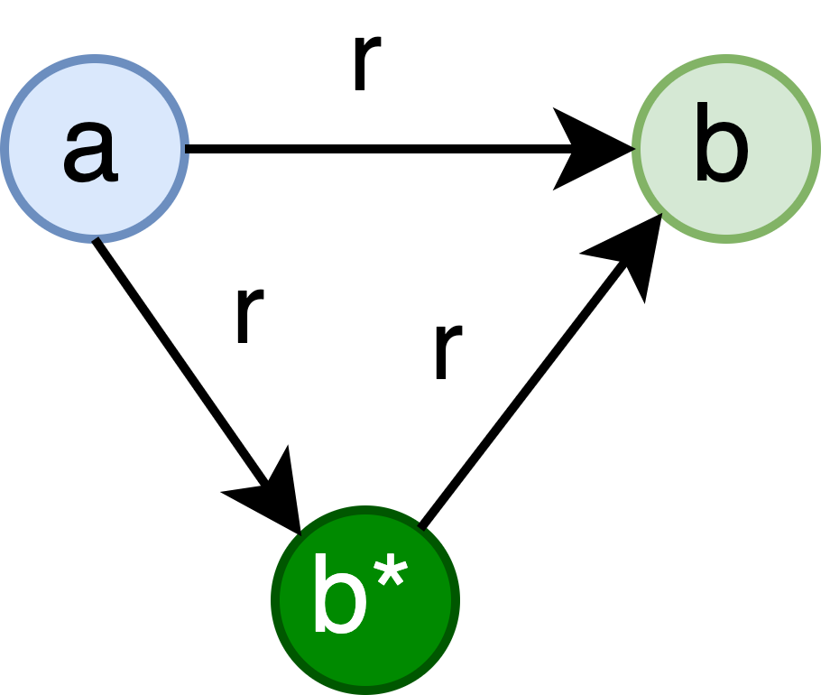
(b) As a part of $P_{\boldsymbol{\sigma}_{b}}$.

Figure 5: Partial representations of $P_{\boldsymbol{\sigma}_{a}}$ and $P_{\boldsymbol{\sigma}_{b}}$.

Similarly, consider a third preference profile $\boldsymbol{\sigma}_{b}$, produced from by cloning $b$ in $\boldsymbol{\sigma}$. Let $b^{*}$ denote the added clone. By definition of clones, we need to have $P_{\boldsymbol{\sigma}_{b}}[a,b^{*}]=r$. Say we choose $P_{\boldsymbol{\sigma}_{b}}[b^{*},b]=r$, in which case the partial graphical representation of $P_{\boldsymbol{\sigma}_{b}}$ would appear as shown in Figure 5(b). Once again, the remaining incoming and outgoing edges from these three nodes (edges that are not shown in the figure) are identical to one another due to the definitions of clones and pseudo-clones.

Comparing Figure 5(a) and Figure 5(b), we see that the two graphs $P_{\boldsymbol{\sigma}_{a}}$ and $P_{\boldsymbol{\sigma}_{b}}$ are isomorphic up to a relabeling of the nodes (specifically relabeling $a^{*}$ as $b^{*}$). Since $h$ is a deterministic function of the pairwise comparison matrix, as shown above, and since $CE_{S}$ satisfies Condition $\boxed{3}$, relabeling of nodes should preserve the output of $h$ up to the same relabelings. In this case, if $h(P_{\boldsymbol{\sigma_{a}}})=\pi_{a}$ and $h(P_{\boldsymbol{\sigma_{b}}})=\pi_{b}$, we must have $\pi^{-1}_{a}(a)=\pi^{-1}_{b}(a)$, $\pi^{-1}_{a}(b)=\pi^{-1}_{b}(b)$, and $\pi^{-1}_{a}(a^{*})=\pi^{-1}_{b}(b^{*})$ by the isomorphism of $P_{\boldsymbol{\sigma_{a}}}$ and $P_{\boldsymbol{\sigma_{b}}}$. Similarly, let $h(P_{\boldsymbol{\sigma}})=\pi$ and let $F$, $F^{a}$ and $F^{b}$ be the lists of eliminated candidates produced by running $CE_{S}$ on $\boldsymbol{\sigma}$, $\boldsymbol{\sigma}_{a}$ and $\boldsymbol{\sigma}_{b}$, respectively. By choosing the original profile $\boldsymbol{\sigma}$ such that all $c\in A\setminus\{a,b\}$ win against $a,b$ (i.e., $P_{\boldsymbol{\sigma}}[c,a]>\frac{n}{2}$ and $P_{\boldsymbol{\sigma}}[c,b]>\frac{n}{2}$) we can ensure that $S[c,a]>S[a,c]$ and $S[c,b]>S[b,c]$ for all $c\in A\setminus\{a,b\}$. This would ensure that the order in which $a$ and $b$ appear in $\pi$ is the same as the order they appear in $F$, that the order in which $a,b$, and $a^{*}$ appear in $\pi_{a}$ is the same as the order they appear in $F^{a}$, and that the order in which $a,b$, and $b^{*}$ appear in $\pi_{b}$ is the same as the order they appear in $F^{b}$, as their their comparisons with other candidates will result in their immediate elimination.

To see how we can use this setup in order to complete our proof, consider an example: suppose that $\pi_{a}=\{(...)a(...)b(...)a^{*}(...)\}$ (i.e., $\pi^{-1}_{a}(a)<\pi^{-1}_{a}(b)<\pi^{-1}_{a}(a^{*})$). Then by the assumption that $CE_{S}$ satisfies condition $\boxed{1}$, we must have $\pi=\{(...)b(...)a(...)\}$ (as this is the order in which $b$ and the last surviving clone of $a$ appear in $\pi_{a}$ and hence in $F^{a}$). Similarly, by the fact that $P_{\boldsymbol{\sigma}_{a}}$ is isomorphic to $P_{\boldsymbol{\sigma}_{b}}$, we must have $\pi_{b}=\{(...)a(...)b(...)b^{*}(...)\}$. However, again by Condition $\boxed{1}$, this would imply $\pi=\{(...)a(...)b(...)\}$ (as this is the order in which $a$ and the last surviving clone of $b$ appear in $\pi_{b}$ and hence in $F^{b}$), which is a contradiction. Hence, we cannot have $h(P_{\boldsymbol{\sigma}_{a}})=\pi_{a}=\{(...)a(...)b(...)a^{*}(...)\}$.

The example above does not rule out other options for $\pi_{a}$, and in fact an ordering such as $h(P_{\boldsymbol{\sigma}_{a}})=\pi_{a}=\{(...)a(...)a^{*}(...)b(...)\}$ would not lead to a contradiction for $r>\frac{n}{2}$. Hence, we now consider a modified preference profile $\boldsymbol{\sigma}^{\prime}$ with pairwise comparison matrix $P_{\boldsymbol{\sigma}^{\prime}}$, where we have $P_{\boldsymbol{\sigma}^{\prime}}[a,b]=P_{\boldsymbol{\sigma}^{\prime}}[b,a]=\frac{n}{2}$ and all other aspects are the same as $\boldsymbol{\sigma}$ (which is equivalent to setting $r=\frac{n}{2}$). Notice that this is indeed possible as long as we set $|N|=n$ to be even. In that case, the edges corresponding to $P[a,b]$ and $P[b,a]$ are symmetric in the the matrix of pairwise comparisons (say $P_{\boldsymbol{\sigma^{\prime}}}$), which can be seen in Figure 6.

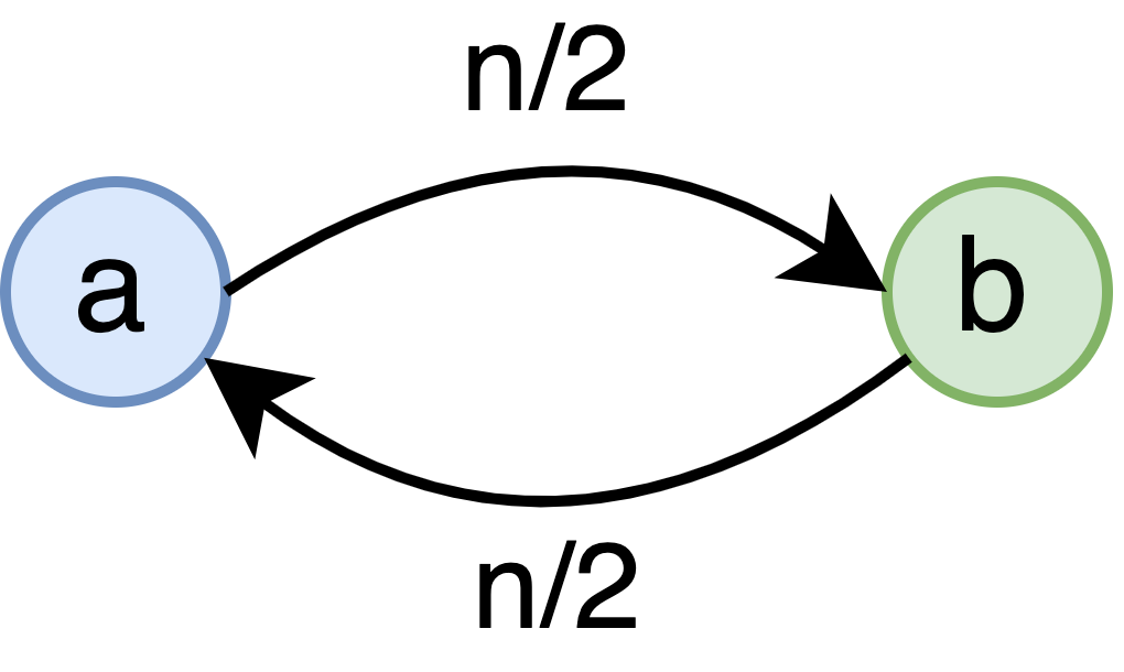
Figure 6: As a part of $P_{\boldsymbol{\sigma}^{\prime}}$.

Once again, consider two new preference profiles $\boldsymbol{\sigma}^{\prime}_{a}$ and $\boldsymbol{\sigma}^{\prime}_{b}$, produced from by cloning $a$ and $b$ in $\boldsymbol{\sigma}$, respectively. Say $a^{*}$ and $b^{*}$ are the the added clones of $a$ and $b$ in $\boldsymbol{\sigma}^{\prime}_{a}$ and $\boldsymbol{\sigma}^{\prime}_{b}$, respectively. By definition of clones, we need to have $P_{\boldsymbol{\sigma}_{a}}[a^{*},b]=P_{\boldsymbol{\sigma}_{a}}[b,a^{*}]=P_{\boldsymbol{\sigma}_{b}}[a,b^{*}]=P_{\boldsymbol{\sigma}_{a}}[b^{*},a]=\frac{n}{2}$. Say we choose $P_{\boldsymbol{\sigma}_{a}}[a,a^{*}]=P_{\boldsymbol{\sigma}_{a}}[b,b^{*}]=r$ for some $r>\frac{n}{2}$, in which case the partial graphical representation of $P_{\boldsymbol{\sigma}^{\prime}_{a}}$ and of $P_{\boldsymbol{\sigma}^{\prime}_{b}}$ would appear as shown in Figures 7(a) and 7(b), respectively. Once again, the remaining incoming and outgoing edges from these three nodes (edges that are not shown in the figure) are identical to one another due to the definitions of clones and pseudo-clones.

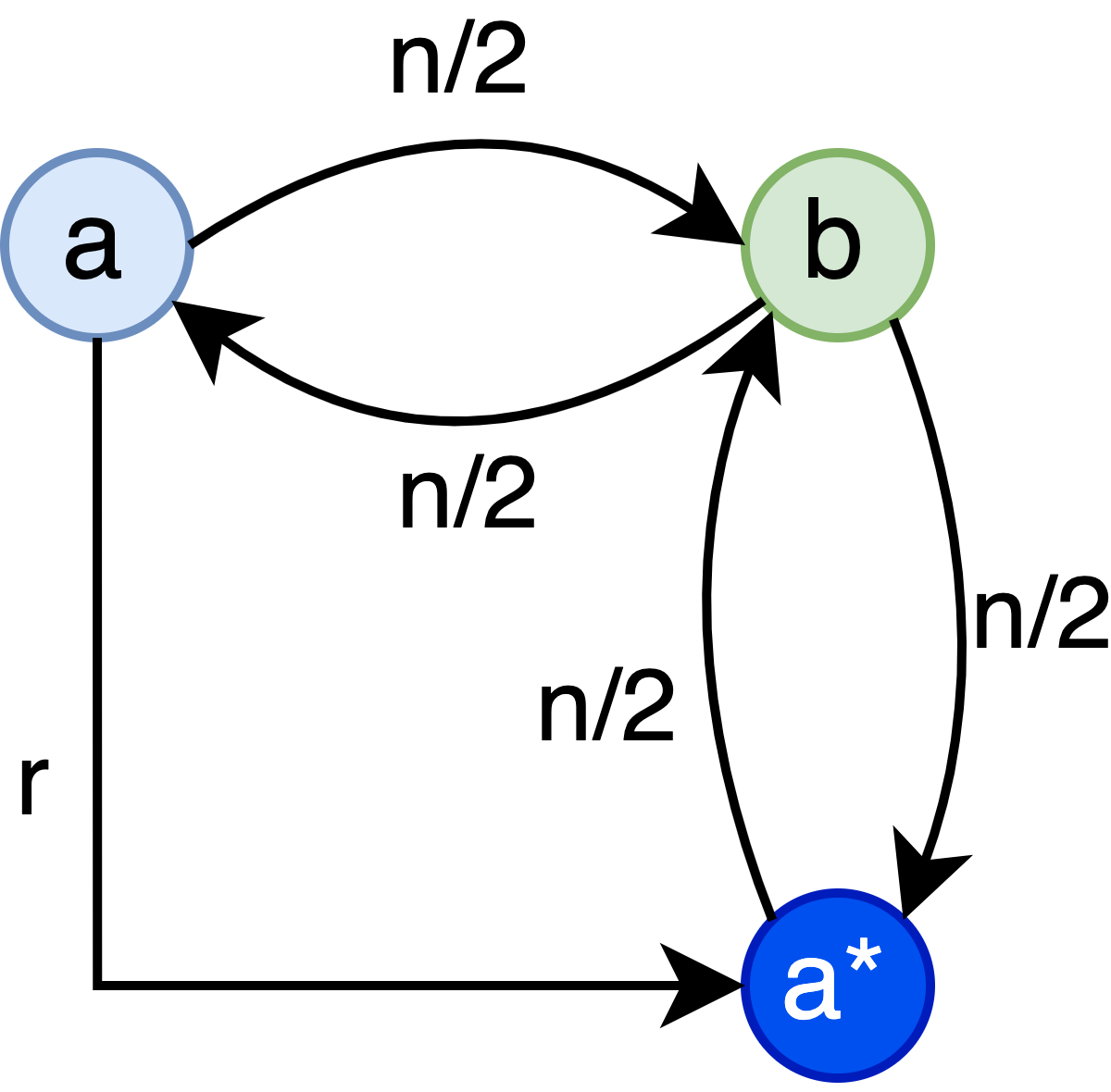
(a) As a part of $P_{\boldsymbol{\sigma}^{\prime}_{a}}$.

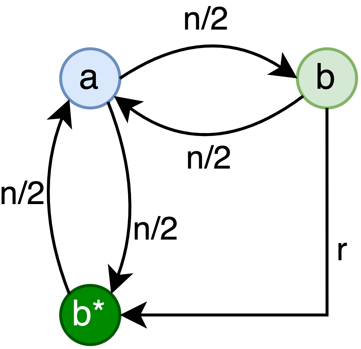
(b) As a part of $P_{\boldsymbol{\sigma}^{\prime}_{b}}$.

Figure 7: Partial representations of $P_{\boldsymbol{\sigma}^{\prime}_{a}}$ and $P_{\boldsymbol{\sigma}^{\prime}_{b}}$.

From Figures 7(a) and 7(b), we can see that the graphs of $P_{\boldsymbol{\sigma}^{\prime}_{a}}$ and $P_{\boldsymbol{\sigma}^{\prime}_{b}}$ are isomorphic. To see this, consider the isomorphism $\phi$ from $P_{\boldsymbol{\sigma}^{\prime}_{a}}$ to $P_{\boldsymbol{\sigma}^{\prime}_{b}}$ where $\phi(a)=b$, $\phi(a^{*})=b^{*}$, $\phi(b)=a$, and $\phi(c)=c$ for all $c\in A\setminus\{a,b\}$. In that case, if $h(P_{\boldsymbol{\sigma_{a}}^{\prime}})=\pi^{\prime}_{a}$ and $h(P_{\boldsymbol{\sigma_{b}}^{\prime}})=\pi^{\prime}_{b}$, we must have $\pi^{\prime-1}_{a}(a)=\pi^{\prime-1}_{b}(b)$, $\pi^{\prime-1}_{a}(a^{*})=\pi^{\prime-1}_{b}(b^{*})$, and $\pi^{\prime-1}_{a}(b)=\pi^{\prime-1}_{b}(a)$. This implies that the order in which $a,b$, and $a^{*}$ appear in $\pi^{\prime}_{a}$ is deterministic on the order in which $a,b$, and $b^{*}$ appear in $\pi^{\prime}_{b}$. Similarly, since $CE_{S}$ satisfies condition $\boxed{1}$, the order in which $a$ and $b$ appear in $h(\boldsymbol{\sigma}^{\prime})=\pi^{\prime}$ must match the order in which $b$ and the last surviving clone of $a$ appear in $\pi^{\prime}_{a}$ and the order in which $a$ and the last surviving clone of $b$ appear in $\pi^{\prime}_{b}$. There are a total of $3!=6$ different orders in which $a,b$, and $a^{*}$ can appear in $\pi^{\prime}_{a}$. Below, we consider each of these cases:

$\pi^{\prime}_{a}$	$\pi^{\prime}_{b}$ (determined from $\pi^{\prime}_{a}$)	$\pi^{\prime}$ (det. from $\pi^{\prime}_{a}$)	$\pi^{\prime}$ (det. from $\pi^{\prime}_{b}$)
$\{(...)a(...)a^{*}(...)b(...)\}$	$\{(...)b(...)b^{*}(...)a(...)\}$	$\{(...)a(...)b(...)\}$	$\{(...)b(...)a(...)\}$
$\{(...)a(...)b(...)a^{*}(...)\}$	$\{(...)b(...)a(...)b^{*}(...)\}$	$\{(...)b(...)a(...)\}$	$\{(...)a(...)b(...)\}$
$\{(...)a^{*}(...)a(...)b(...)\}$	$\{(...)b^{*}(...)b(...)a(...)\}$	$\{(...)a(...)b(...)\}$	$\{(...)b(...)a(...)\}$
$\{(...)a^{*}(...)b(...)a(...)\}$	$\{(...)b^{*}(...)a(...)b(...)\}$	$\{(...)b(...)a(...)\}$	$\{(...)a(...)b(...)\}$
$\{(...)b(...)a(...)a^{*}(...)\}$	$\{(...)a(...)b(...)b^{*}(...)\}$	$\{(...)b(...)a(...)\}$	$\{(...)a(...)b(...)\}$
$\{(...)b(...)a^{*}(...)a(...)\}$	$\{(...)a(...)b^{*}(...)b(...)\}$	$\{(...)b(...)a(...)\}$	$\{(...)a(...)b(...)\}$

Comparing the third and fourth columns, we see that the order of $a$ and $b$ in $\pi^{\prime}$ required to match $\pi^{\prime}_{a}$ contradicts with the order of $a$ and $b$ in $\pi^{\prime}$ required to match $\pi^{\prime}_{b}$ for all rows. This implies that there is no function $h$ that, when applied to $\boldsymbol{\sigma}^{\prime},\boldsymbol{\sigma}^{\prime}_{a},\boldsymbol{\sigma}^{\prime}_{b}$, satisfies Condition $\boxed{4}$ for both $\boldsymbol{\sigma}^{\prime}_{a}$ and $\boldsymbol{\sigma}^{\prime}_{b}$. This is a contradiction to the assumption that $CE_{S}$ satisfies Condition $\boxed{4}$ (as if it did, this condition should have held for all preference profiles). Thus, $CE_{S}$ is not a clocked election, implying that the Schultze Method cannot be implemented as a clocked election. Thus, the Schultze Method is not Obviously Independent of Clones.

∎

Appendix D Examples

D.1 STV Examples (with and without clones)

8	5	4	3	1
Voters	Voters	Voters	Voters	Voters
b	a	c	d	a
a	c	d	b	c
c	b	b	a	d
d	d	a	c	b

The order of elimination is as follows: $[d,c,a]$. The winner is $b$.

8	5	4	3	1
Voters	Voters	Voters	Voters	Voters
b	a	cx	d	a
a	c	c	b	c
cx	cx	d	a	cx
c	b	b	cx	d
d	d	a	c	b

The order of elimination is as follows: $[c,d,cx,a]$. The winner is $b$.

8	5	4	3	1
Voters	Voters	Voters	Voters	Voters
b	a	cx	d	a
bx	c	c	bx	c
a	cx	d	b	cx
cx	b	b	a	d
c	bx	bx	cx	bx
d	d	a	c	b

The order of elimination is as follows: $[bx,c,d,cx,a]$. The winner is $b$.

Note that the orders of elimination given above for these three preference profiles correspond to the order in which the protocol $CE_{STV}$ given in Definition 4.1 would eliminate the candidates when given these preference profiles as an input. Comparing the three lists, we see that the last surviving clones of each candidate always appear in the order $[d,c,a]$, confirming that $CE_{STV}$ does indeed satisfy Condition 1 from Definition 3.2 in this example.

D.2 Example run of Ranked Pairs (with and without Clones)

Consider the following voter profile:

10	8	6	5	3	1
Voters	Voters	Voters	Voters	Voters	Voters
d	b	a	c	d	a
a	a	c	d	b	c
b	c	b	b	a	d
c	d	d	a	c	b

The corresponding majority matrix is:

	a	b	c	d
a	0	1	23	-3
b	-1	0	9	-5
c	-23	-9	0	7
d	3	5	-7	0

Using the majority matrix we add the edges in the following order:

$$\{ac,bc,cd,\cancel{db},\cancel{da},ab\}$$

Where we remove directed edges $db$ and $da$ as they cause a cycle to form. This leaves us with the following graph:

As node $a$ is the source, $a$ is declared the winner.

Furthermore, the Ranked Pairs voting algorithm is provably independent of clones; the full proof can be found in the paper by [Tid87]. To illustrate some of the intuition behind this, consider the following example where $c$ is cloned into $c$ and $cx$.

10	8	6	5	3	1
Voters	Voters	Voters	Voters	Voters	Voters
d	b	a	cx	d	a
a	a	c	c	b	cx
b	c	cx	d	a	c
cx	cx	b	b	cx	d
c	d	d	a	c	b

The corresponding majority matrix is:

	a	b	c	cx	d
a	0	1	23	23	-3
b	-1	0	9	9	-5
c	-23	-9	0	-5	7
cx	-23	-9	5	0	7
d	3	5	-7	-7	0

Using the majority matrix we add the edges in the following order:

$$\{acx,ac,bcx,bc,cxd,cd,\cancel{db},cxc,\cancel{da},ab\}$$

Where we remove directed edges $db$ and $da$ as they cause a cycle to form. This leaves us with the graph shown in Figure 8.

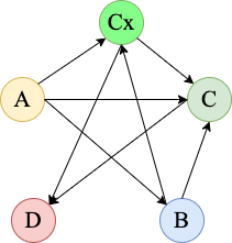
Figure 8: Graph during the execution of the Ranked Pairs algorithm with clones.

Since node $a$ is the source, $a$ is declared the winner.

Notice that based on the order in which the edges are added in each preference profile, we see that the order of eliminated candidates that $CE_{RP}$ (defined in Definition 4.4) would produce when given the original and the clones preference profile are $F=\{c,d,b\}$ and $F^{\prime}=\{cx,c,d,b\}$. Note that the order in which the last surviving clone of each set of clones appear on both lists is $\{c,d,b\}$, demonstrating that $CE_{RP}$ does indeed satisfy Condition $\boxed{1}$ of Definition 3.2 in this example.

D.3 Example run of Schulze method (with and without clones)

Consider the following voter profile:

8	2	4	4	3
Voters	Voters	Voters	Voters	Voters
a	b	c	d	d
c	a	d	b	c
d	d	b	a	b
b	c	a	c	a

The corresponding pairwise matrix is:

$P$	a	b	c	d
a	0	8	14	10
b	13	0	6	2
c	7	15	0	12
d	11	19	9	0

Which generates the strength matrix:

$S$	a	b	c	d
a	0	(14,7)	(14,7)	(12,9)
b	(13,8)	0	(13,8)	(12,9)
c	(13,8)	(15,6)	0	(12,9)
d	(13,8)	(19,2)	(13,8)	0

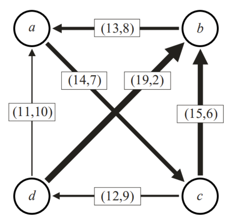
Figure 9: The graph generated by this voter profile as depicted by [Sch18].

Therefore, as denoted by the graph, the winner is d. The Schulze voting method is also independent of clones [Sch11]. To illustrate, consider the following example where d is cloned into d and dx.

8	2	4	4	3
Voters	Voters	Voters	Voters	Voters
a	b	c	dx	d
c	a	dx	d	dx
dx	d	d	b	c
d	dx	b	a	b
b	c	a	c	a

The corresponding pairwise matrix is:

$P$	a	b	c	d	dx
a	0	8	14	10	10
b	13	0	6	2	2
c	7	15	0	12	12
d	11	19	9	0	5
dx	11	19	9	16	0

Which generates the strength matrix:

$S$	a	b	c	d	dx
a	0	(14,7)	(14,7)	(12,9)	(12,9)
b	(13,8)	0	(13, 8)	(12,9)	(12, 9)
c	(13,8)	(15,6)	0	(12,9)	(12, 9)
d	(13,8)	(13,8)	(19,2)	0	(12, 9)
dx	(13, 8)	(13, 8)	(19, 2)	(16, 5)	0

This gives us the winner $d$, which maintains the independence of clones. However, notice that we have determined $d$ without requiring an order of eliminated candidates. For this reason, the Schulze method does not satisfy the conditions required in a Clocked Election (Definition 3.2). This stands in stark contrast with Examples D.1 and D.2, which demonstrates the intuition behind the fact that STV and RP are OiOC but the Schulze method is not, which we formally prove in Theorems 4.2, 4.5, and 4.7.

References

- [AG18] Itai Ashlagi and Yannai A Gonczarowski. Stable matching mechanisms are not obviously strategy-proof. Journal of Economic Theory, 177:405–425, 2018.
- [BL07] Scott Bennett and Rob Lundie. Australian electoral systems. Parliament of Australia. Department of Parliamentary Services, 2007.
- [EFS10] Edith Elkind, Piotr Faliszewski, and Arkadii Slinko. Cloning in elections. Proceedings of the AAAI Conference on Artificial Intelligence, 24(1):768–773, Jul. 2010.
- [EFS11] Edith Elkind, Piotr Faliszewski, and Arkadii M. Slinko. Clone structures in voters’ preferences. CoRR, abs/1110.3939, 2011.
- [FBC14] Rupert Freeman, Markus Brill, and Vincent Conitzer. On the axiomatic characterization of runoff voting rules. Proceedings of the AAAI Conference on Artificial Intelligence, 28(1), Jun. 2014.
- [FV17] Diodato Ferraioli and Carmine Ventre. Obvious strategyproofness needs monitoring for good approximations. In Thirty-First AAAI Conference on Artificial Intelligence, 2017.
- [GHT22] Yannai A Gonczarowski, Ori Heffetz, and Clayton Thomas. Strategyproofness-exposing mechanism descriptions. arXiv preprint arXiv:2209.13148, 2022.
- [GL21] Louis Golowich and Shengwu Li. On the computational properties of obviously strategy-proof mechanisms. arXiv preprint arXiv:2101.05149, 2021.
- [Li17] Shengwu Li. Obviously strategy-proof mechanisms. American Economic Review, 107(11):3257–87, 2017.
- [Lin17] Yehuda Lindell. How to simulate it–a tutorial on the simulation proof technique. Tutorials on the Foundations of Cryptography, pages 277–346, 2017.
- [PX12] David C Parkes and Lirong Xia. A complexity-of-strategic-behavior comparison between schulze’s rule and ranked pairs. In Twenty-Sixth AAAI Conference on Artificial Intelligence, 2012.
- [Sch11] Markus Schulze. A new monotonic, clone-independent, reversal symmetric, and condorcet-consistent single-winner election method. Social choice and Welfare, 36(2):267–303, 2011.
- [Sch18] Markus Schulze. The schulze method of voting. arXiv preprint arXiv:1804.02973, 2018.
- [Sec21] Secretary of State and Needham, Andrew. State of Oregon, Nov 2021.
- [SVWX21] Krzysztof Sornat, Virginia Vassilevska Williams, and Yinzhan Xu. Fine-grained complexity and algorithms for the schulze voting method. In Proceedings of the 22nd ACM Conference on Economics and Computation, pages 841–859, 2021.
- [Tid87] Nicolaus Tideman. Independence of clones as a criterion for voting rules. Social Choice and Welfare, 4(3):185–206, 1987.
- [Tro19] Peter Troyan. Obviously strategy-proof implementation of top trading cycles. International Economic Review, 60(3):1249–1261, 2019.