PoGaIN: Poisson-Gaussian Image Noise
Modeling from Paired Samples

Abstract

Image noise can often be accurately fitted to a Poisson-Gaussian distribution. However, estimating the distribution parameters from a noisy image only is a challenging task. Here, we study the case when paired noisy and noise-free samples are accessible. No method is currently available to exploit the noise-free information, which may help to achieve more accurate estimations. To fill this gap, we derive a novel, cumulant-based, approach for Poisson-Gaussian noise modeling from paired image samples. We show its improved performance over different baselines, with special emphasis on MSE, effect of outliers, image dependence, and bias. We additionally derive the log-likelihood function for further insights and discuss real-world applicability.

I Introduction

Noise always affects image capture in any imaging pipeline. Modeling noise distribution is thus crucial for analyzing imaging devices, datasets [1, 2], and developing denoising methods, especially blind ones [3, 4, 5, 6]. Those approaches include noise parameter estimation prior to the noise reduction, and hence do not rely on the noise level being known. Other learning-based techniques even go a step further and are noise model-blind, meaning that no fixed noise model is imposed [7, 8]. Here, we assume a common noise model, the Poisson-Gaussian noise model, composed of a shot and a read noise component. The former is modeled with a Poisson distribution, emerging from the particle nature of light whose intensity the sensor estimates over a finite duration of time. The latter is modeled with a Gaussian distribution, notably for raw images that are processed by the different steps in the image processing pipeline, which can modify the distribution.

In their seminal work, Foi et al. [9] also propose a Poisson-Gaussian model for the noise distribution. Further, the authors introduce a clever solution for fitting the noise model parameters from a noisy input image. Their algorithm begins with local expectation and standard deviation estimates from image parts that are assumed to depict a single underlying intensity value. The global parametric model is then fitted through a maximum likelihood search based on the local estimates. Multiple assumptions are made in order to reach a final estimate, in part due to the lack of input information beyond the noisy image. Our premise is that when modeling datasets or analyzing an imaging system, we may be able to acquire paired noisy and noise-free images. We exploit this additional information and study the problem of modeling noise with paired samples.

We propose a novel method that estimates the parameters of the aforementioned noise model based on noisy and noise-free image pairs that can be used to develop new blind denoising algorithms. The additional information of the noise-free version of a given image enables our approach to significantly outperform the method introduced by Foi et al. [9]. We also train a neural network based noise model estimator and show that we in addition outperform this learning-based alternative. Finally, for the sake of comparison, we introduce a variance-based baseline method, which also takes advantage of noisy and noise-free image pairs.

II Related work

Denoising is one of the most fundamental tasks in image restoration, with both theoretical impact and practical applications. Most classic denoisers, for instance PURE-LET [10], KSVD [11], WNNM [12], BM3D [13], and EPLL [14], require knowledge of the noise level in the input test image. Deep learning image denoisers that have shown improved empirical performance [15, 16] also require knowledge of noise distributions, if not at test time [17], then at least for training [3, 18]. This is due to the degradation overfitting of deep neural networks [19]. Noise modeling is thus important for denoisers at test time, but also for acquisition system analysis and dataset modeling for training these denoisers. Past research has focused on modeling noise from noisy images without relying on ground truth, i.e., noise-free, information [9]. Interesting approaches, for example Sparse Modeling [20], Dictionary Learning [21] or non-local image denoising methods like SAFPI [22], have been developed to push overall denoising performance. However, none of these methods allow easy use of noise-free data when it is available. For Poisson-Gaussian noise modeling, for example, both FMD [1] and W2S [2] rely on a noise modeling method that does not consider ground truth noise-free images [9]. Hence, our approach to model the Poisson-Gaussian Image Noise (PoGaIN) distribution exploits paired samples (noisy and noise-free images), which significantly improves the modeling accuracy. Our method is based on the cumulant expansion, which is also used by other authors to derive estimators for PoGaIN model parameters, but for different input types, such as noisy image time series [23] or single noisy images [24].

III Mathematical formulation

III-A Poisson-Gaussian model

The Poisson-Gaussian noise model proposed by Foi et al. [9] consists of two components, the Poisson shot noise and the Gaussian read noise, which are assumed to be independent. The signal-dependent Poisson component $\eta_{p}$ and signal-independent Gaussian component $\eta_{g}$ are defined, respectively, by

$$\eta_{p}=\frac{1}{a}\alpha,\quad\eta_{g}=\beta,\quad\alpha\sim\mathcal{P}(ax),\quad\beta\sim\mathcal{N}(0,b^{2}),$$ (1)

where $x$ is the ground truth (noise-free) signal, and $a$ and $b$ are distribution parameters. The complete model is made up of the sum of these two components

$$y=\eta_{p}+\eta_{g}=\frac{1}{a}\alpha+\beta,$$ (2)

where $y$ is the observed (noisy) signal. We note to the reader that the $a$ and $b$ in [9] correspond to our $a^{-1}$ and our $b^{2}$, respectively. Thus, our $a$ is equal to the quantum efficiency in percent.

As derived in the supplementary material, the following properties hold for $\eta_{p}$

$$\mathbb{E}[\eta_{p}]=x,\quad\mathbb{V}[\eta_{p}]=\frac{x}{a},$$ (3)

which shows that the Poisson component is indeed signal-dependent and that the Gaussian component, having constant mean and variance, is signal independent. Consequently, we derive the expected value and variance of the observation $y$

$$\mathbb{E}[y]=x,\quad\mathbb{V}[y]=\frac{x}{a}+b^{2}.$$ (4)

III-B Likelihood derivation

The noise model, presented in Equation (2), leads to the following expression for the likelihood

$$\mathcal{L}(y|a,b,x)=\prod_{i}\sum_{k=0}^{\infty}\frac{(ax_{i})^{k}}{k!b\sqrt{2\pi}}\exp{\left(-ax_{i}-\frac{(y_{i}-k/a)^{2}}{2b^{2}}\right)},$$ (5)

where $y$ is the captured noisy image, $x$ is the ground truth noise-free image and $i$ is the pixel index in the vectorized representation of an image. The complete derivation of the likelihood function is given in the supplementary material.

The noise parameters $\hat{a}$ and $\hat{b}$ that optimize for the maximum likelihood are then given by

$$\begin{split}\hat{a},\hat{b}=\arg\max_{a,b}\mathcal{L}(y|a,b,x).\end{split}$$ (6)

Optimizing over the log-likelihood $\mathcal{LL}$ is computationally inefficient. To improve convergence, we truncate the summation over $k$ to a $k_{max}$ such that most of the weight of the sum lies in $k$ values below $k_{max}$ (details in code). Nonetheless, optimizing $\mathcal{LL}$ is not a viable solution to our problem. However, as we show in our Analysis V-D2, the log-likelihood can still provide empirical insight.

IV Proposed method

Rather than interpreting $x$ and $y$ as two observed images, we consider $x$ and $y$ as a collection of samples from two distributions $\mathcal{X}$ and $\mathcal{Y}$ and define a random variable $X\sim\mathcal{X}$ such that

$$\mathbb{P}[X=x_{i}]=\frac{\left|\set{k:x_{k}=x_{i}}\right|}{n},$$ (7)

where $n$ corresponds to the number of samples (i.e., the number of pixels in $x$ and $y$). We define $\mathcal{Y}$ to be the distribution of the Poisson-Gaussian noise model over the distribution $\mathcal{X}$. Formally, introducing another random variable $Y\sim\mathcal{Y}$, we get

$$Y\sim\mathcal{Y}=\frac{\mathcal{P}(a\mathcal{X})}{a}+\mathcal{N}(0,b^{2}).$$ (8)

Next, we obtain the $2$-nd and $3$-rd cumulant of $\mathcal{Y}$ as a system of equations

$$\begin{split}\left\{\begin{array}[]{l}\kappa_{2}[\mathcal{Y}]=\frac{\overline{x}}{a}+\overline{x^{2}}-\overline{x}^{2}+b^{2}\\ \kappa_{3}[\mathcal{Y}]=\overline{x^{3}}-3\overline{x^{2}}\overline{x}+2\overline{x}^{3}+3\frac{\overline{x^{2}}}{a}-3\frac{\overline{x}^{2}}{a}+\frac{\overline{x}}{a^{2}}\end{array}\right.,\end{split}$$ (9)

where $\overline{x}$ denotes the mean of $x$ (for example $\overline{x^{k}}^{j}=(\frac{1}{n}\sum_{i}x_{i}^{k})^{j}$). Both $\kappa_{2}[\mathcal{Y}]$ and $\kappa_{3}[\mathcal{Y}]$ can be estimated with an unbiased estimator (k-statistic). Therefore, Equations (9) form a system of two equations, with two unknowns, $a$ and $b$, which is solved by our cumulant-based method (OURS).

V Experimental evaluation

V-A Data processing

The dataset we use is based on the Berkeley Segmentation Dataset 300 [25]. We synthesize noise stochastically by picking a seed $s\in\set{0,\dots,9}$, $a\in[1,100]$ and $b\in[0.01,0.15]$ and distort images from the training set [25] with it, resulting in noisy and noise-free image pairs. For validation, we pick $10$ images out of the test set of [25]. For each seed $s\in\set{0,\dots,9}$, and for $25$ linearly spaced values for $a\in[1,100]$ and $b\in[0.01,0.15]$, we synthesize an image pair, resulting in a total of $62500$ pairs for evaluation.

V-B Baseline methods

V-B1 FOI

The method proposed by Foi et al. [9] estimates $a$ and $b$ by segmenting pixels assumed to have the same underlying value but to be distorted by noise into non-overlapping intensity level sets. Further, a local estimation of multiple expectation and standard-deviation pairs is carried out. Finally, a global parametric model fitting using those local estimates is performed. FOI only uses $y$, and does not provide a way to exploit $x$ even if it is available. Naturally, that makes a good estimation of $a$ and $b$ more challenging.

V-B2 CNN

For the sake of comparison, we design a convolutional neural network (CNN) that we train to predict $a$ and $b$. The detailed architecture of the CNN is described in our code repository. The CNN takes only the noisy image $y$ as input. We cannot rule out that a more complex neural network based solution could outperform this CNN. We provide it as an additional baseline, and it is not the focus of this article.

V-B3 VAR

For fairness of comparison, we design a baseline method that also takes advantage of noisy and noise-free image pairs. To derive it, we define $Y_{i}=\set{y_{j}:x_{j}=x_{i}}$ as the set of all pixels of $y$ for which the corresponding pixels in $x$ have the same intensity as $x_{i}$. This approach is based on the variance across the pixel sets $Y_{i}$. First, the theoretical mean of $Y_{i}$ is $x_{i}$, and hence we can compute the empirical variance of $Y_{i}$

$$\mathbb{V}[Y_{i}]=\frac{1}{\left|Y_{i}\right|}\sum_{y_{k}\in Y_{i}}(y_{k}-x_{i})^{2}.$$ (10)

Additionally, $y_{j}\sim\frac{\mathcal{P}(ax_{i})}{a}+\mathcal{N}(0,b^{2})$. Thus, according to Equation (4), $\mathbb{V}[Y_{i}]\approx\frac{x_{i}}{a}+b^{2}$. Using this observation, we select $a,b$ such that the above approximation holds as closely as possible between the two values for any given $i$, where $\mathbb{V}[Y_{i}]$ is computed using Equation (10). Finally, we obtain an estimation of $a,b$ by computing

$$\hat{a},\hat{b}=\arg\min_{a,b}{\sum_{i}\left(\mathbb{V}[Y_{i}]-\frac{x_{i}}{a}-b^{2}\right)^{2}}.$$ (11)

In our experiments, images have 8-bit depth, and thus we only have 256 possible values for $x_{i}$. Hence, we can expect that sufficiently many pixels share the same intensity. However, this assumption limits this method, because it relies on images that have a few different pixel intensities, i.e., a sparse histogram, and that have a large dynamic range to get robust empirical variance values $\mathbb{V}[Y_{i}]$. Further, note that in Equation (11), the same intensity level $x_{i}$ is appearing in the sum $\left|Y_{i}\right|$ times, and thus introduces a bias.

V-C Experimental results

First, we provide results statistics of the Mean Squared Error (MSE) for the estimates ${\hat{a}}^{-1},{\hat{b}}^{2}$ of the different methods compared to the ground truth values $a^{-1},b^{2}$ in Tables I and II.

TABLE I: Statistics about the MSE error on ${\hat{a}}^{-1}$ for various methods.

Method	Mean	Standard Dev.	75%-Quantile	Maximum
FOI	$3147.703\,950$	$746\,292.063\,221$	$0.000\,564$	$186\,467\,350.054\,470$
CNN	$0.017\,767$	$0.086\,703$	$0.000\,074$	$0.633\,754$
VAR	$0.000\,008$	$0.000\,085$	$\boldsymbol{\approx}$ $0$	$0.003\,535$
OURS	$0.000\,003$	$0.000\,014$	$0.000\,001$	$0.000\,277$

TABLE II: Statistics about the MSE error on ${\hat{b}}^{2}$ for various methods.

Method	Mean	Standard Dev.	75%-Quantile	Maximum
FOI	$0.346\,023$	$6.674\,889$	$0.000\,094$	$615.874\,927$
CNN	$0.000\,008$	$0.000\,023$	$0.000\,005$	$0.000\,387$
VAR	$0.000\,001$	$0.000\,011$	$\boldsymbol{\approx}$ $0$	$0.000\,445$
OURS	$\boldsymbol{\approx}$ $0$	$0.000\,001$	$\boldsymbol{\approx}$ $0$	$0.000\,033$

In our experimental setting, FOI performs worst compared to the other methods. This is expected, as the method only uses noisy observations $y$. That is the same for the CNN, which, however, performs better. Thus, for most of the following graphs and plots, we only focus on our method OURS compared with the baseline methods CNN and VAR.

V-C1 Mean squared error

The MSE on ${\hat{a}}^{-1}$ is inversely correlated to the value of $a$, as shown in Fig. 1. This fact can be explained by the dependence of our noise model on $a^{-1}$. For small $a$, the Poisson noise component is dominant. But when $a$ increases, the Poisson contribution to the noise model gradually vanishes. The MSE on ${\hat{b}}^{2}$ does not depend significantly on $b$, it is roughly constant for all methods except CNN. Nonetheless, instances with less overall noise (large $a$ and small $b$) lead in general to smaller MSE values.

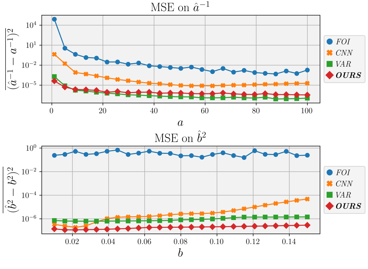
Figure 1: MSE for each method as a function of $a$ (top) and $b$ (bottom). Note that the error axis is in log scale.

We note that our method consistently outperforms CNN. Additionally, we also see that OURS achieves a roughly $10$ times smaller MSE value on ${\hat{b}}^{2}$ than VAR, while VAR slightly improves MSE on ${\hat{a}}^{-1}$, particularly for larger $a$.

V-C2 Effect of outliers and image dependence

We analyze the effect that outliers have on the overall performance of the different methods. We consider samples as outliers when $\text{MSE}>Q(0.75)+1.5*(Q(0.75)-Q(0.25))$ where $Q(0.25)$ and $Q(0.75)$ are the first and the third quartiles, respectively. We remove those outlier values, and Table III shows the percentage of data remaining after filtering. In Fig. 2 we show the performance on 10 images [25], with and without outliers. Excluding outliers significantly improves the performance.

TABLE III: Percentage of data not eliminated as outliers.

Method	$a$-based outliers	$b$-based outliers	Combined
CNN	$0.821\,664\text{\times}{10}^{2}\text{\,}\mathrm{\char 37\relax}$	$0.841\,392\text{\times}{10}^{2}\text{\,}\mathrm{\char 37\relax}$	$0.701\,776\text{\times}{10}^{2}\text{\,}\mathrm{\char 37\relax}$
VAR	$0.851\,600\text{\times}{10}^{2}\text{\,}\mathrm{\char 37\relax}$	$0.857\,357\text{\times}{10}^{2}\text{\,}\mathrm{\char 37\relax}$	$0.819\,280\text{\times}{10}^{2}\text{\,}\mathrm{\char 37\relax}$
OURS	$0.878\,112\text{\times}{10}^{2}\text{\,}\boldsymbol{\mathrm{\char 37\relax}}$	$0.889\,520\text{\times}{10}^{2}\text{\,}\boldsymbol{\mathrm{\char 37\relax}}$	$0.828\,320\text{\times}{10}^{2}\text{\,}\boldsymbol{\mathrm{\char 37\relax}}$

We can further observe that MSE varies depending on the intrinsic properties of the noise-free images $x$. We illustrate this dependence of the MSE in Fig. 2 by averaging over all different seeds and over the $a$ or $b$ values, respectively. One can observe that the ground truth image more significantly influences the estimation performance for the $b$ parameter. Additionally, we note that OURS is the most robust when it comes to causing outlier error values, whereas CNN is most prone to producing outliers.

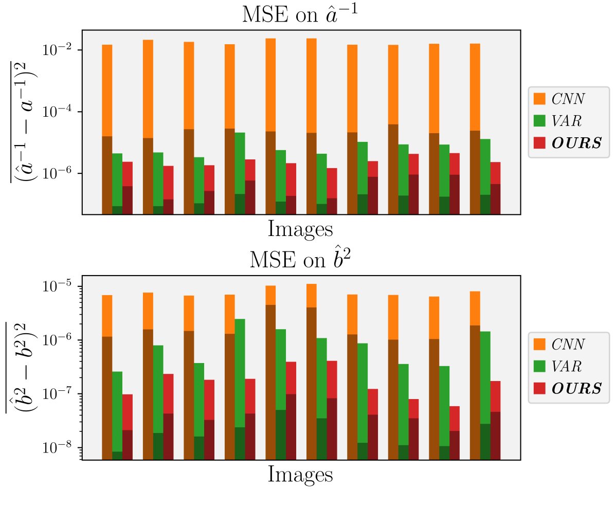
Figure 2: MSE dependence on $10$ images for ${\hat{a}}^{-1}$ (top) and ${\hat{b}}^{2}$ (bottom), including outliers (bright colors) and excluding outliers (dark colors). Note that the error axis is in log scale.

V-D Analysis

V-D1 Bias

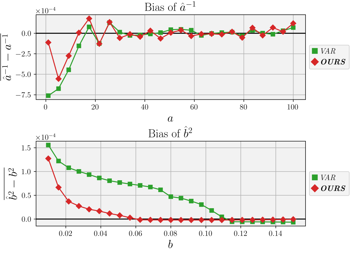
Figure 3: Absolute estimation error, illustrating the bias in ${\hat{a}}^{-1}$ (top) and ${\hat{b}}^{2}$ (bottom) of estimators VAR and OURS, for varying $a,b$ values. Note that the bias axis is in linear scale.

Fig. 3 shows that the bias is most significant for both the smallest values of $a$ and of $b$, although the bias is small in general. For OURS and ${\hat{a}}^{-1}$, this bias is explained by the variance of $\kappa_{3}[\mathcal{Y}]$ in Equation (9), as this variance is dependent on $a^{-1}$ and is larger when $a$ is small. Further, the bias on ${\hat{b}}^{2}$ comes from the fact that we only keep real values of $\hat{b}$, discarding negative estimates of ${\hat{b}}^{2}$. By eliminating negative estimates, we introduce a positive bias. For VAR, Equation (11) shows that under-estimating ${\hat{b}}^{2}$ leads to an over-estimation of ${\hat{a}}^{-1}$, which highlights the challenging un-mixing of the two noise parameters in this setup. Fig. 3 also shows that VAR is always biased in $b$ while for OURS the bias is zero for $b>0.06$.

V-D2 Log-likelihood

As discussed in section V-D2, $\mathcal{LL}$ cannot be efficiently optimized for global minima. However, empirically, $\mathcal{LL}$ can give additional insight. In Fig. 4, we show the relative absolute difference between $\mathcal{LL}$ for the actual values $a,b$ and their estimates $\hat{a},\hat{b}$ averaged over the validation images and seeds for different methods; $\overline{\left|\frac{\mathcal{LL}(y|\hat{a},\hat{b},x)-\mathcal{LL}(y|a,b,x)}{\mathcal{LL}(y|a,b,x)}\right|}$.

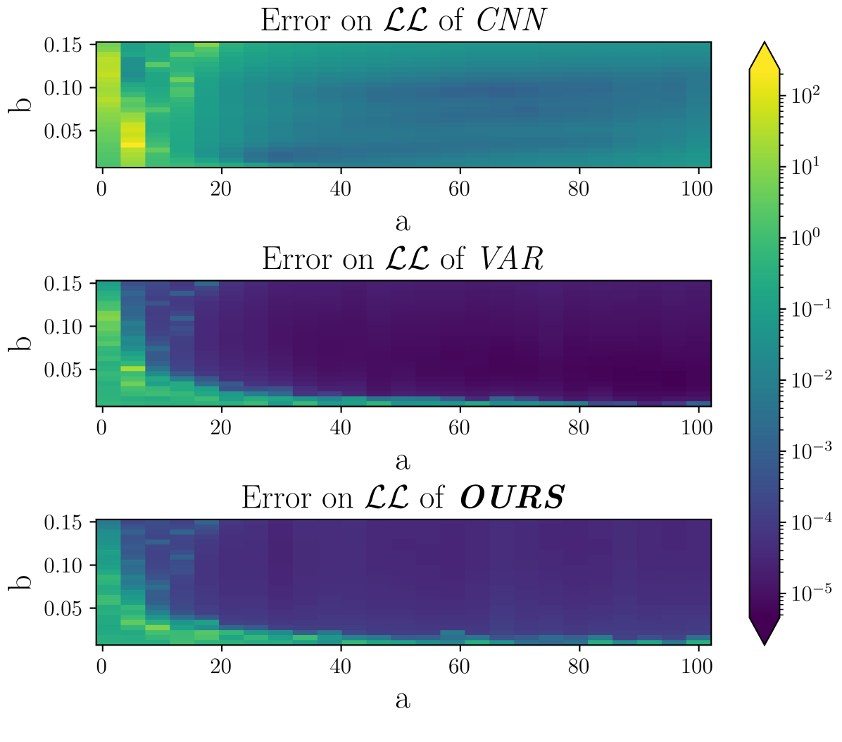
Figure 4: Relative absolute difference between the $\mathcal{LL}$ computed for the estimated parameters, and the actual $\mathcal{LL}$ of the ground truth parameters. Note that the error axis is in log scale.

As shown in Fig. 4, CNN leads to the biggest error. Moreover, VAR results in estimates that are more “likely” on average, but, as shown earlier, performs worse than OURS. This is due to the complexity of the statistical distribution of the noise model, leading to a mismatch between likelihood-maximization and expected-error-minimization estimators.

V-D3 Real-world scenario

For real-world applications, the Poisson component often dominates the noise model ($a$ is small). OURS achieves smaller MSE than VAR when $a$ is small. Therefore, while VAR can provide more accurate $a$ estimates in certain cases, in real-world applications OURS outperforms this baseline. Further, OURS is more robust to outlier errors, is less biased, and consistently achieves smaller MSE on ${\hat{b}}^{2}$. VAR also relies on images having a sparse histogram and a large dynamic range. For all these reasons, OURS is better suited for real-world applications.

VI Conclusion

We propose an efficient cumulant-based Poisson-Gaussian noise estimator for paired noisy and noise-free images. Our method significantly outperforms prior baselines, notably a neural network solution and a variance-based method, both of which we design. Finally, the log-likelihood that we derive enables us to demonstrate the intrinsic difficulty of the Poisson-Gaussian noise estimation.

In future work, one could explore fine-tuning the weights of the VAR baseline and taking into account the clipping behavior of digital sensors in real-world applications. Furthermore, we note that our method can be used as a starting point to speed up the optimization for maximizing the likelihood function that we derive, if likelihood —rather than inverse expected error— is to be maximized.

References

- [1] Y. Zhang, Y. Zhu, E. Nichols, Q. Wang, S. Zhang, C. Smith, and S. Howard, “A Poisson-Gaussian denoising dataset with real fluorescence microscopy images,” in Proceedings of the IEEE/CVF Conference on Computer Vision and Pattern Recognition, 2019, pp. 11 710–11 718.
- [2] R. Zhou, M. El Helou, D. Sage, T. Laroche, A. Seitz, and S. Süsstrunk, “W2S: microscopy data with joint denoising and super-resolution for widefield to SIM mapping,” in European Conference on Computer Vision Workshops, 2020, pp. 474–491.
- [3] M. El Helou and S. Süsstrunk, “Blind universal Bayesian image denoising with Gaussian noise level learning,” IEEE Transactions on Image Processing, vol. 29, pp. 4885–4897, 2020.
- [4] L. D. Tran, S. M. Nguyen, and M. Arai, “GAN-based noise model for denoising real images,” in Proceedings of the Asian Conference on Computer Vision, 2020.
- [5] X. Liu, M. Tanaka, and M. Okutomi, “Single-image noise level estimation for blind denoising,” IEEE Transactions on Image Processing, vol. 22, no. 12, pp. 5226–5237, 2013.
- [6] J. Fang, S. Liu, Y. Xiao, and H. Li, “Sar image de-noising based on texture strength and weighted nuclear norm minimization,” Journal of Systems Engineering and Electronics, vol. 27, no. 4, pp. 807–814, 2016.
- [7] T. Ehret, A. Davy, J.-M. Morel, G. Facciolo, and P. Arias, “Model-blind video denoising via frame-to-frame training,” in 2019 IEEE/CVF Conference on Computer Vision and Pattern Recognition (CVPR), 2019, pp. 11 361–11 370.
- [8] S. Zhu, G. Xu, Y. Cheng, X. Han, and Z. Wang, “Bdgan: Image blind denoising using generative adversarial networks,” in Pattern Recognition and Computer Vision, Z. Lin, L. Wang, J. Yang, G. Shi, T. Tan, N. Zheng, X. Chen, and Y. Zhang, Eds. Cham: Springer International Publishing, 2019, pp. 241–252.
- [9] A. Foi, M. Trimeche, V. Katkovnik, and K. Egiazarian, “Practical Poissonian-Gaussian noise modeling and fitting for single-image raw-data,” IEEE Transactions on Image Processing, vol. 17, no. 10, pp. 1737–1754, 2008.
- [10] F. Luisier, T. Blu, and M. Unser, “Image denoising in mixed Poisson-Gaussian noise,” IEEE Transactions on Image Processing, vol. 20, no. 3, pp. 696–708, 2011.
- [11] M. Aharon, M. Elad, and A. Bruckstein, “K-SVD: An algorithm for designing overcomplete dictionaries for sparse representation,” IEEE Transactions on Signal Processing, vol. 54, no. 11, pp. 4311–4322, 2006.
- [12] S. Gu, L. Zhang, W. Zuo, and X. Feng, “Weighted nuclear norm minimization with application to image denoising,” in Computer Vision and Pattern Recognition (CVPR), 2014.
- [13] K. Dabov, A. Foi, V. Katkovnik, and K. Egiazarian, “Image denoising by sparse 3-D transform-domain collaborative filtering,” IEEE Transactions on Image Processing, vol. 16, no. 8, pp. 2080–2095, 2007.
- [14] D. Zoran and Y. Weiss, “From learning models of natural image patches to whole image restoration,” in International Conference on Computer Vision (ICCV), 2011.
- [15] T. Huang, S. Li, X. Jia, H. Lu, and J. Liu, “Neighbor2Neighbor: A self-supervised framework for deep image denoising,” IEEE Transactions on Image Processing, 2022.
- [16] X. Ma, X. Lin, M. El Helou, and S. Süsstrunk, “Deep Gaussian denoiser epistemic uncertainty and decoupled dual-attention fusion,” in IEEE International Conference on Image Processing (ICIP), 2021, pp. 1–4.
- [17] K. Zhang, W. Zuo, and L. Zhang, “FFDNet: Toward a fast and flexible solution for CNN-based image denoising,” IEEE Transactions on Image Processing, vol. 27, no. 9, pp. 4608–4622, 2018.
- [18] M. El Helou and S. Süsstrunk, “BIGPrior: Towards decoupling learned prior hallucination and data fidelity in image restoration,” IEEE Transactions on Image Processing, 2022.
- [19] M. El Helou, R. Zhou, and S. Süsstrunk, “Stochastic frequency masking to improve super-resolution and denoising networks,” in European Conference on Computer Vision (ECCV), 2020, pp. 749–766.
- [20] Q. Wang, X. Zhang, Y. Wu, L. Tang, and Z. Zha, “Nonconvex weighted minimization based group sparse representation framework for image denoising,” IEEE Signal Processing Letters, vol. 24, no. 11, pp. 1686–1690, 2017.
- [21] S. Cai, Z. Kang, M. Yang, X. Xiong, C. Peng, and M. Xiao, “Image denoising via improved dictionary learning with global structure and local similarity preservations,” Symmetry, vol. 10, no. 5, p. 167, May 2018. [Online]. Available: http://dx.doi.org/10.3390/sym10050167
- [22] S. Cai, K. Liu, M. Yang, J. Tang, X. Xiong, and M. Xiao, “A new development of non-local image denoising using fixed-point iteration for non-convex sparse optimization,” PLOS ONE, vol. 13, no. 12, pp. 1–24, 12 2018. [Online]. Available: https://doi.org/10.1371/journal.pone.0208503
- [23] A. Jezierska, H. Talbot, C. Chaux, J.-C. Pesquet, and G. Engler, “Poisson-gaussian noise parameter estimation in fluorescence microscopy imaging,” in 2012 9th IEEE International Symposium on Biomedical Imaging (ISBI), 2012, pp. 1663–1666.
- [24] B. Zhang, “Contributions to fluorescence microscopy in biological imaging: PSF modeling, image restoration, and super-resolution detection,” Ph.D. dissertation, Télécom ParisTech, Informatics, telecommunications and electronics (EDITE), Paris, France, Nov. 2007. [Online]. Available: https://pastel.archives-ouvertes.fr/pastel-00003273
- [25] D. Martin, C. Fowlkes, D. Tal, and J. Malik, “A database of human segmented natural images and its application to evaluating segmentation algorithms and measuring ecological statistics,” in Proc. 8th Int’l Conf. Computer Vision, vol. 2, July 2001, pp. 416–423.