Phenotype switching in chemotaxis aggregation models controls the spontaneous emergence of large densities

Abstract

We consider a phenotype-switching chemotaxis model for aggregation, in which a chemotactic population is capable of switching back and forth between a chemotaxing state (performing chemotactic movement) and a secreting state (producing the attractant). We show that the switching rate provides a powerful mechanism for controlling the densities of spontaneously emerging aggregates. Specifically, in two- and three-dimensional settings it is shown that when both switching rates coincide and are suitably large, then the densities of both the chemotaxing and the secreting population will exceed any prescribed level at some points in the considered domain. This is complemented by two results asserting the absence of such aggregation phenomena in corresponding scenarios in which one of the switching rates remains within some bounded interval.
Key words: chemotaxis; indirect signal production; singularity formation
MSC 2020: 35B44 (primary); 35B36, 35B45, 35K55, 92C17 (secondary)

1 Introduction

The Keller-Segel system for chemotactic movement [12] constitutes a classical model of mathematical biology, noted for its capacity to exhibit self-organisation. When formulated with two variables – a chemotactic population and its diffusive chemoattractant – and making the assumption that the population secretes its own attractant, positive feedback is inserted into this system that allows clusters to form through self-reinforcement. Studies of this system form a significant literature, ranging from biological and sociological applications of the model [19] to studies into the intricate analytical properties [8, 2]. In terms of the latter, resolving the question of whether solutions to the system exist globally-in-time or blow up has been of particular interest.

This simple model implicitly assumes homogeneity across the population, i.e. that all members have equivalent capacity to perform chemotaxis and/or produce attractant. These assumptions of homogeneity, however, can lie at odds with the heterogeneity observed in natural systems, where a population will often span a spectrum of phenotypes, such as variable chemotactic sensitivity in the context of chemotactic behaviour [22]. The presence of phenotypic heterogeneity may confer numerous advantages, such as adaptability within fluctuating environments, but must also be considered within the wider context of energy balances [11]: performing one activity (e.g. movement) has an inevitable energy cost, meaning less resources may be available for other activities (e.g. protein synthesis and transport), i.e. there exists a trade-off. In light of this, recent models have been developed that extend the Keller and Segel framework to include phenotypic heterogeneity and trade-offs, either through a population that spans a continuous spectrum of phenotypes [17] or a population subdivided into discrete phenotypic states [18]. The latter considered a self-organisation type scenario, specifically focusing on a trade-off in which the population either performed chemotaxis (chemotaxing state) or produced the attractant (secreting state), but could not perform both simultaneously. Linear stability analysis of this model demonstrated that pattern formation is possible, but that the rate of switching between the two states becomes a crucial factor in the dynamics. Numerical analyses confirmed these predictions and, moreover, hinted that solutions exist globally-in-time, yet a formal analysis was not attempted.

Motivated by this, we will focus on a family of problems based on the system introduced in [18]. In the following, $u_{\alpha\beta}$ represents the chemotaxing phenotype, $w_{\alpha\beta}$ represents the secreting phenotype and $v_{\alpha\beta}$ is the chemoattractant. Specifically, we shall consider the problems

$$\left\{\begin{array}[]{ll}\partial_{t}u_{\alpha\beta}=\Delta u_{\alpha\beta}-\nabla\cdot(u_{\alpha\beta}\nabla v_{\alpha\beta})-\alpha u_{\alpha\beta}+\beta w_{\alpha\beta},&x\in\Omega,\ t>0,\\[2.84526pt] \partial_{t}v_{\alpha\beta}=\Delta v_{\alpha\beta}-v_{\alpha\beta}+w_{\alpha\beta},&x\in\Omega,\ t>0,\\[2.84526pt] \partial_{t}w_{\alpha\beta}=\Delta w_{\alpha\beta}-\beta w_{\alpha\beta}+\alpha u_{\alpha\beta},&x\in\Omega,\ t>0,\\[2.84526pt] \frac{\partial u_{\alpha\beta}}{\partial\nu}=\frac{\partial v_{\alpha\beta}}{\partial\nu}=\frac{\partial w_{\alpha\beta}}{\partial\nu}=0,&x\in\partial\Omega,\ t>0,\\[2.84526pt] u_{\alpha\beta}(x,0)=u_{0}(x),\quad v_{\alpha\beta}(x,0)=v_{0}(x),\quad w_{\alpha\beta}(x,0)=w_{0}(x),&x\in\Omega,\end{array}\right.$$ (1.1)

with $\alpha>0$ and $\beta>0$ representing the rate of switching from chemotaxing to secreting and secreting to chemotaxing, respectively.

Viewed from a mathematical perspective, (1.1) differs from the corresponding initial-boundary value problem for the classical Keller-Segel system

$$\left\{\begin{array}[]{l}u_{t}=\Delta u-\chi\nabla\cdot(u\nabla v),\\[2.84526pt] v_{t}=\Delta v-v+\mu u,\end{array}\right.$$ (1.2)

by including a form of indirectness with respect to the signal production process. Whereas the classical system is well-known for its ability to generate unbounded densities within the chemotaxing population ([7], [26]), the inclusion of indirectness within the signal dynamics has been found to significantly reduce a trend toward singular destabilisation. In particular, in [6] the presence of additional diffusion-induced dissipation of the form in (1.1) was shown to suppress any blow-up phenomena in a closely related problem in three (and lower)-dimensional settings. Meanwhile, a substantial collection of additional studies has provided comparable findings for a number of nearby extensions ([3], [16], [21], [29], [30], [31], [32]). Lacking, as far as we are aware, is a rigorous understanding into the extent to which regularised systems of this nature retain core features of taxis-driven destabilisation, despite the absence of unboundedness phenomena.
Main results. The purpose of the present manuscript is to confirm that the coefficients $\alpha$ and $\beta$ of the zero order contributions to (1.1) play a key role in this regard. In particular, simultaneously increasing these parameters can result in the spontaneous emergence of structures which, while not singular, do lead to population densities of arbitrary size.
As a preliminary step, in Section 3 we confirm that, within frameworks of physically relevant dimension, blow-up does not occur in any of the populations in (1.1), in the sense that for any choice of the parameters therein, and for all reasonably regular nonnegative initial data, a global bounded classical solution can always be found:

Proposition 1.1

Let $n\leq 3$ and $\Omega\subset\mathbb{R}^{n}$ be a bounded domain with smooth boundary, let $\alpha>0$ and $\beta>0$, and suppose that

$$u_{0}\in W^{1,\infty}(\Omega),v_{0}\in W^{1,\infty}(\Omega)\mbox{ and }w_{0}\in W^{1,\infty}(\Omega)\quad\mbox{are nonnegative}.$$ (1.3)

Then there exist uniquely determined nonnegative functions

$$\left\{\begin{array}[]{l}u_{\alpha\beta}\in C^{0}(\overline{\Omega}\times[0,\infty))\cap C^{2,1}(\overline{\Omega}\times(0,\infty)),\\[2.84526pt] v_{\alpha\beta}\in\bigcap_{q>n}C^{0}([0,\infty);W^{1,q}(\Omega))\cap C^{2,1}(\overline{\Omega}\times(0,\infty))\qquad\mbox{and}\\[2.84526pt] w_{\alpha\beta}\in C^{0}(\overline{\Omega}\times[0,\infty))\cap C^{2,1}(\overline{\Omega}\times(0,\infty))\end{array}\right.$$ (1.4)

such that $(u_{\alpha\beta},v_{\alpha\beta},w_{\alpha\beta})$ forms a classical solution of (1.1). Moreover, this solution is bounded in the sense that for each $q>n$ there exists $C(q)>0$ such that

$$\|u_{\alpha\beta}(\cdot,t)\|_{L^{\infty}(\Omega)}+\|v_{\alpha\beta}(\cdot,t)\|_{W^{1,q}(\Omega)}+\|w_{\alpha\beta}(\cdot,t)\|_{L^{\infty}(\Omega)}\leq C(q)\qquad\mbox{for all }t>0.$$ (1.5)

In the light of a corresponding result for a relative of (1.1), obtained in [6], this observation is not in itself particularly surprising. The approach taken to derive this, however, is designed in such a way that it can be artlessly further developed so as to reveal that the bounds in (1.5) are actually uniform within large parts of the parameter region $(0,\infty)^{2}$.
In fact, as a first statement in this direction, we show that provided $\alpha$ is located in a fixed interval, then the inequality in (1.5) remains stable for arbitrarily large $\beta$:

Proposition 1.2

Let $n\leq 3$, and assume (1.3). Then for each $q>n$ and any $\alpha^{\star}>0$ and $\delta>0$, there exists $C(q,\alpha^{\star},\delta)>0$ such that

$$\|u_{\alpha\beta}(\cdot,t)\|_{L^{\infty}(\Omega)}+\|v_{\alpha\beta}(\cdot,t)\|_{W^{1,q}(\Omega)}+\|w_{\alpha\beta}(\cdot,t)\|_{L^{\infty}(\Omega)}\leq C(q,\alpha^{\star},\delta)$$

for all $$t>0 \alpha\in(0,\alpha^{\star}] \beta\geq\delta$$ and any choice of and . (1.6)

Likewise, under the corresponding scenario that $\beta$ is located in a fixed interval, unboundedness phenomena can also be ruled out in the limit $\alpha\to\infty$:

Proposition 1.3

Let $n\leq 3$, and suppose that (1.3) holds. Then whenever $q>n,\beta^{\star}>0$ and $\delta\in(0,\beta^{\star})$, one can find $C(q,\beta^{\star},\delta)>0$ with the property that

$$\|u_{\alpha\beta}(\cdot,t)\|_{L^{\infty}(\Omega)}+\|v_{\alpha\beta}(\cdot,t)\|_{W^{1,q}(\Omega)}+\|w_{\alpha\beta}(\cdot,t)\|_{L^{\infty}(\Omega)}\leq C(q,\beta^{\star},\delta)$$

$$\hskip 85.35826pt\qquad\mbox{for all $t>0$, any $\alpha>0$ and each }\beta\in[\delta,\beta^{\star}].$$ (1.7)

In stark contrast to the above results, however, our final result will indicate that when both parameters in (1.1) simultaneously diverge, then arbitrarily large population densities may spontaneously emerge in two- and three-dimensional balls. To address this in as simple as possible setting, we shall concentrate here on the prototypical case when the large numbers $\alpha$ and $\beta$ precisely coincide, and hence consider the one-parameter sub-family of (1.1) given by

$$\left\{\begin{array}[]{ll}\partial_{t}u_{\gamma}=\Delta u_{\gamma}-\nabla\cdot(u_{\gamma}\nabla v_{\gamma})-\gamma u_{\gamma}+\gamma w_{\gamma},&x\in\Omega,\ t>0,\\[2.84526pt] \partial_{t}v_{\gamma}=\Delta v_{\gamma}-v_{\alpha\beta}+w_{\gamma},&x\in\Omega,\ t>0,\\[2.84526pt] \partial_{t}w_{\gamma}=\Delta w_{\gamma}-\gamma w_{\gamma}+\gamma u_{\gamma},&x\in\Omega,\ t>0,\\[2.84526pt] \frac{\partial u_{\gamma}}{\partial\nu}=\frac{\partial v_{\gamma}}{\partial\nu}=\frac{\partial w_{\gamma}}{\partial\nu}=0,&x\in\partial\Omega,\ t>0,\\[2.84526pt] u_{\gamma}(x,0)=u_{0}(x),\quad v_{\gamma}(x,0)=v_{0}(x),\quad w_{\gamma}(x,0)=w_{0}(x),&x\in\Omega,\end{array}\right.$$ (1.8)

with $\gamma>0$.
Within this context, for some fixed initial data the corresponding solutions can be seen to undergo a quite drastic unboundedness phenomenon, as to be confirmed in Section 4:

Theorem 1.4

Let $n\in\{2,3\},R>0$ and $\Omega=B_{R}(0)\subset\mathbb{R}^{n}$. Then there exist $T>0$ and radially symmetric initial data which satisfy (1.3), and which are such that whenever $(\gamma_{j})_{j\in\mathbb{N}}\subset(0,\infty)$ is unbounded, one can find a subsequence $(\gamma_{j_{k}})_{k\in\mathbb{N}}$ with the property that for the corresponding solutions of (1.8) from Proposition 1.1 we have

$$\|u_{\gamma_{j_{k}}}\|_{L^{\infty}(\Omega\times(0,T))}\to\infty\qquad\mbox{as }k\to\infty$$ (1.9)

and

$$\|w_{\gamma_{j_{k}}}\|_{L^{\infty}(\Omega\times(0,T))}\to\infty\qquad\mbox{as }k\to\infty.$$ (1.10)

We remark here that the taxis-driven spontaneous emergence of large densities has been discovered within extreme parameter constellations for several Keller-Segel type systems. However, unlike the majority of preceding literature in this regard (cf., e.g. [15], [10], [4], [24], [27] or [28]), the observation that leads to Theorem 1.4 does not refer to parameter limits which are singular in the sense that either fast or slow diffusion limits are involved; indeed, the underlying core mechanism here appears to be more complex, in that the dominance of chemotaxis over diffusion is enforced by an enhanced zero order interaction, despite the marked non-degeneracy of all migration processes.

2 Numerical motivation

To motivate Propositions 1.1-1.3 and Theorem 1.4 we compare numerical solutions of the switching model (1.8) with those of the formulation

$$\left\{\begin{array}[]{ll}\partial_{t}u_{\infty}=\Delta u_{\infty}-\frac{1}{2}\nabla\cdot(u_{\infty}\nabla v_{\infty}),&x\in\Omega,\ t>0,\\[2.84526pt] \partial_{t}v_{\infty}=\Delta v_{\infty}-v_{\infty}+\frac{1}{2}u_{\infty},&x\in\Omega,\ t>0,\\[2.84526pt] \frac{\partial u_{\infty}}{\partial\nu}=\frac{\partial v_{\infty}}{\partial\nu}=0,&x\in\partial\Omega,\ t>0,\\[2.84526pt] u_{\infty}(x,0)=u_{0}(x),\quad v_{\infty}(x,0)=v_{0}(x),&x\in\Omega,\end{array}\right.$$ (2.1)

The above can be regarded as the classical companion to (1.8), featuring a homogeneous population, $u_{\infty}$, that secretes its own chemoattractant, $v_{\infty}$. A standard linear stability analysis of the uniform steady state solutions for (2.1) predicts that self-organisation can occur, given sufficient population mass. However, subsequent dynamics vary according to the dimension, $n$: when $n=1$ solutions exist globally-in-time, yet when $n\geq 2$ finite-time blow-up can occur. Intuitively, (2.1) could conceivably arise in the limit $\gamma\rightarrow\infty$ of (1.8): switching between chemotaxis-only and secreting-only states becomes instantaneous, effectively generating a single-state population that simultaneously produces the attractant and performs chemotaxis; the half-factors reflect a division of time between the two states.

To substantiate this intuition we perform a numerical exploration for $n=1,2,3$. Generally, numerical studies in $n=2,3$ are compromised by computational cost, particularly if high accuracy is required. To circumvent this such that simulations in $n=1,2,3$ can be performed to an equivalent degree of resolution, each of the cases $n=2,3$ are restricted to an assumed radial symmetry. Specifically, for $n=1$ we consider the interval $\Omega=[0,R]$, while in $n=2,3$ we consider $\Omega={\cal{B}}_{R}^{n}$ (the $n$-dimensional ball of radius $R$) and radially symmetric initial data, allowing reduction to the radial line $[0,R]$. All simulations utilise the initial distributions $u_{\gamma}(x,0)=w_{\gamma}(x,0)=\rho/2$, $v_{\gamma}(x,0)=\rho(1+0.001e^{-x^{2}})/2$ for (1.8) or $u_{\infty}(x,0)=\rho$, $v_{\infty}(x,0)=\rho(1+0.001e^{-x^{2}})/2$ for (2.1); here, $x$ is used to refer to either the position along the interval $[0,R]$ in $n=1$, or the radial position in $n=2,3$. The parameter $\rho$ measures the population mass and linear stability analysis (see [18]) can be used to determine the autoaggregation parameter spaces. Specifically, these are regions in $(R,\rho,\gamma)$-space for (1.8) and $(R,\rho)$-space for (2.1) in which the uniform steady state is unstable to the inhomogeneous perturbation and aggregations are predicted to emerge. Regarding the numerical implementation itself, we utilise the pdepe solver in Matlab, which discretises in space to yield a system of ODEs to be integrated in time (using ode15s). The above initial conditions bias high density aggregate emergence to the origin, which can then be exploited by performing a spatial discretisation on a non-uniform mesh. Specifically we discretise $[0,R]$ into a mesh of $N+1$ points $X_{0},X_{1},\ldots,X_{N}$, where $X_{i}=Ri^{2}/N^{2}$. This concentrates grid points near the origin, where high resolution is desirable for the potentially steep gradients forming at the point of mass concentration. We set $N=10^{4}$ and note that simulations with twice or half the number yielded quasi-identical results. Regardless of these measures, computation of $z(x,t)$ is still expected to fail in certain instances, for example due to emergence of extremely large densities; this is particular to be expected in (2.1) for $n=2,3$, where finite time blow up is possible. Any such scenarios of numerical failure are classified as “numerical blow-up” and we compute up to the critical time $t_{c}$ at which the numerical scheme fails.

We first consider the case $n=1$, see Figure 1. Note that instead of plotting individual variables, we consider the total population density $z(x,t)$, i.e. $z_{\gamma}=u_{\gamma}+w_{\gamma}$ for (1.8) and $z_{\infty}=u_{\infty}$ for (2.1). When $n=1$ we expect global existence for (2.1). Selecting parameters from the autoaggregation parameter space for (2.1), we correspondingly observe the growth of a cluster (Figure 1, dotted-red line) at the boundary $x=0$ and converging towards a high density aggregate; the dotted red-line in Figure 1 (right) shows the long-term solution to (2.1), computed at a point when negligible solution change is observed. Similar dynamics are observed for the switching model (1.8), with the various solid blue-shaded lines in Figure 1 corresponding to distinct choices for $\gamma$. For smaller $\gamma$ the aggregate grows over a slower timescale and settles towards a nonuniform steady state with lower peak density, this delay/reduction resulting from the cost of switching between chemotaxis-only and producing-only states. Note that when $\gamma$ is reduced below a critical threshold, autoaggregation is not possible and solutions rather evolve towards the uniform steady state (see [18] for details). As $\gamma$ is increased, however, faster growth of the cluster occurs and we observe convergence in both space and time between the numerical solutions to (1.8) and those of (2.1). This provides substance to our intuition that (1.8) converges to (2.1) as $\gamma\rightarrow\infty$.

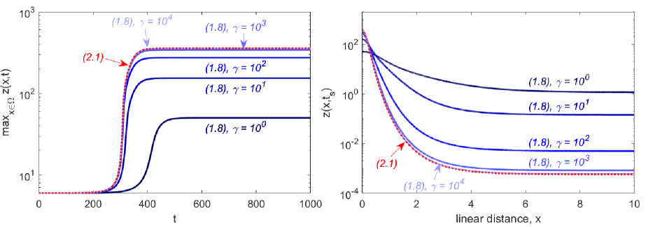
Figure 1: Numerical solutions for (1.8) and (2.1) when $n=1$. Left. Time-evolution of the maximum total population density, $\max_{x\in\Omega}z(x,t)$. Dotted red line shows the solution to (2.1), while blue shaded solid lines indicate solutions to (1.8) with different choices for $\gamma$. Right. Total population density distribution at $t=t_{s}$, i.e. $z(x,t_{s})$, where $t_{s}$ is a point in time at which there is negligible change to the solution (numerical steady state). For these simulations we set $R=10$ and $\rho=6$, with initial conditions as stated in the text.

We next explore the $n=2$ case. Standard theory predicts that solutions to (2.1) will blow-up in finite-time given sufficient initial mass. Correspondingly, upon simulation of (2.1) we observe the initial growth of a cluster that rapidly accelerates into a highly concentrated peak: the growth of this peak is indicated by the red dotted line in Figure 2 (left). Numerical blow-up occurs at $t_{c}\sim 272.269$, beyond which no computation is possible within the limits of the numerical scheme invoked. In stark contrast, corresponding solutions to (1.8) appear to exist globally in-time and no numerical blow-up was observed across the range of $\gamma$ used (five orders of magnitude). Tracking the maximum density of the cluster, we observe a similar initial trend in which the cluster first increases slowly before entering a phase of rapidly accelerating growth. Notably, increasing $\gamma$ leads to a convergence between solutions to (1.8) and solutions to (2.1) prior to $t=t_{c}$, with the time of most rapid acceleration in cluster growth for (1.8) coinciding with the numerical blow-up time observed for (2.1). Beyond this point, however, the growth rate of the clusters that form in (1.8) is curtailed, and solutions begin to converge to what appear to be bounded nonuniform steady state solutions. To quantify this, we plot the maximum density of the steady state cluster distribution that forms for (1.8) as a function of $\gamma$, Figure 2 (right). For larger $\gamma$ we observe an almost perfectly linear relationship between the size of $\gamma$ and the maximum density, implying that there is no clear upper bound to the maximum density of solutions to (1.8) if $\gamma$ is allowed to become arbitrarily high.

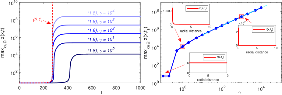
Figure 2: Numerical solutions for (1.8) and (2.1) when $n=2$, assuming radial symmetry. Left. Time-evolution of the maximum total population density, $\max_{x\in\Omega}z(x,t)$. Dotted red line shows the solution to (2.1), while blue shaded solid lines indicate solutions to (1.8) using different choices for $\gamma$. Note that the numerical solution of (2.1) fails at $t_{c}\sim 272.269$ (numerical blow-up). Right. Maximum of the total population density distribution at $t=t_{s}$, i.e. $\max_{x\in\Omega}z(x,t_{s})$, where $t_{s}$ is a point in time at which there is negligible change to the solution (numerical steady state). The insets show the total population density distribution at the same time point, $z(x,t_{s})$, for selected $\gamma$. Note further that the straight line fit through the data for values $\gamma\geq 10^{1}$ is shown via the dotted cyan line. For these simulations we set $L=10$ and $\rho=6$, with initial conditions as stated in the text.

As a final control, we repeat the numerical simulations for the case $n=3$. The results largely mirror those observed for $n=2$, where we observe that while numerical blow-up occurs for the system (2.1) (here, for $t_{c}\sim 276.756$), solutions to (1.8) instead evolve to a tightly aggregated solution with a bounded upper density. As for $n=2$, increasing $\gamma$ leads to a convergence between solutions to the model (1.8) and the solutions to (2.1) prior to the time of numerical blow up. Note that the solution densities formed in $n=3$ are notably higher than those observed in $n=2$ for the corresponding value of $\gamma$. Despite this, however, the numerical solver was still able to compute solutions for (1.8) without numerical blow-up, with growth of the cluster slowing and the solution stabilising into a tightly aggregated steady state solution.

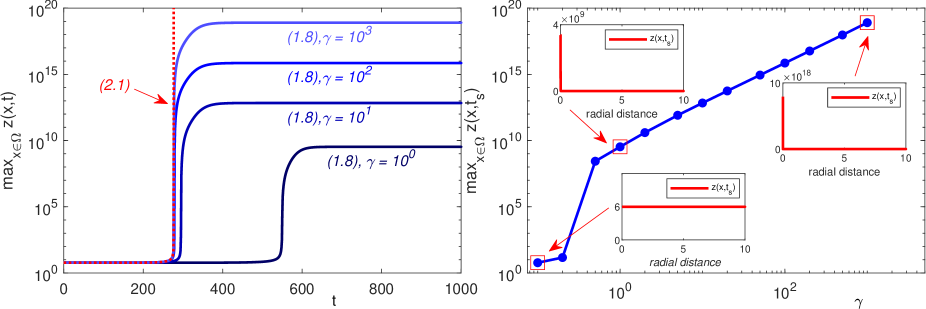
Figure 3: Numerical solutions for (1.8) and (2.1) when $n=3$, assuming radial symmetry. Left. Time-evolution of the maximum total population density, $\max_{x\in\Omega}z(x,t)$. Dotted red line shows the solution to (2.1), while blue shaded solid lines indicate solutions to (1.8) using different choices for $\gamma$. Note that the numerical solution of (2.1) fails at $t_{c}\sim 276.757$ (numerical blow-up). Right. Maximum of the total population density distribution at $t=t_{s}$, i.e. $\max_{x\in\Omega}z(x,t_{s})$, where $t_{s}$ is a point in time at which there is negligible change to the solution (numerical steady state). The insets show the total population density distribution at the same time point, $z(x,t_{s})$, for selected $\gamma$. For these simulations we set $R=10$ and $\rho=6$, with initial conditions as stated in the text.

3 Boundedness results. Proofs of Propositions 1.1, 1.2 and 1.3

3.1 Local existence. Basic properties of $u_{\alpha\beta}+w_{\alpha\beta}$

Let us first recall some standard theory on short-term solvability in triangular taxis-type parabolic systems ([1], [9]) to state, without further comment, the following result on local existence and extensibility of solutions to the general problem (1.1), along with some simple observations concerned with the sum of the corresponding two population densities addressed therein.

Lemma 3.1

Let $n\geq 1$, assume (1.3), and let $\alpha>0$ and $\beta>0$. Then there exist $T_{max}(\alpha,\beta)\in(0,\infty]$ and a classical solution $(u_{\alpha\beta},v_{\alpha\beta},w_{\alpha\beta})$ of (1.1) in $\Omega\times(0,T_{max}(\alpha,\beta))$, uniquely determined by the inclusions

$$\left\{\begin{array}[]{l}u_{\alpha\beta}\in C^{0}(\overline{\Omega}\times(0,T_{max}(\alpha,\beta)))\cap C^{2,1}(\overline{\Omega}\times(0,T_{max}(\alpha,\beta))),\\[2.84526pt] v_{\alpha\beta}\in\bigcap_{q>n}C^{0}([0,T_{max}(\alpha,\beta));W^{1,q}(\Omega))\cap C^{2,1}(\overline{\Omega}\times(0,T_{max}(\alpha,\beta)))\qquad\mbox{and}\\[2.84526pt] w_{\alpha\beta}\in C^{0}(\overline{\Omega}\times(0,T_{max}(\alpha,\beta)))\cap C^{2,1}(\overline{\Omega}\times(0,T_{max}(\alpha,\beta))),\end{array}\right.$$

such that $u_{\alpha\beta}\geq 0,v_{\alpha\beta}\geq 0$ and $w_{\alpha\beta}\geq 0$ in $\Omega\times(0,T_{max}(\alpha,\beta))$, and that

if $$T_{max}(\alpha,\beta)<\infty$$,   then (3.2)

$$\hskip 17.07164pt\limsup_{t\nearrow T_{max}(\alpha,\beta)}\Big{\{}\|u(\cdot,t)\|_{L^{\infty}(\Omega)}+\|v(\cdot,t)\|_{W^{1,q}(\Omega)}+\|w(\cdot,t)\|_{L^{\infty}(\Omega)}\Big{\}}=\infty\quad\mbox{for all $q>n$.}$$ (3.3)

Moreover,

$$z_{\alpha\beta}(x,t):=u_{\alpha\beta}(x,t)+w_{\alpha\beta}(x,t),\qquad x\in\overline{\Omega},\ t\in[0,T_{max}(\alpha,\beta)),$$ (3.4)

satisfies

$$\left\{\begin{array}[]{ll}\partial_{t}z_{\alpha\beta}=\Delta z_{\alpha\beta}-\nabla\cdot(u_{\alpha\beta}\nabla v_{\alpha\beta}),&x\in\Omega,\ t\in(0,T_{max}(\alpha,\beta)),\\[2.84526pt] \frac{\partial z_{\alpha\beta}}{\partial\nu}=0,&x\in\partial\Omega,\ t\in(0,T_{max}(\alpha,\beta)),\\[2.84526pt] z_{\alpha\beta}(x,0)=u_{0}(x)+w_{0}(x),&x\in\Omega,\end{array}\right.$$ (3.5)

and we have

$$\int_{\Omega}z_{\alpha\beta}(\cdot,t)=\int_{\Omega}u_{0}+\int_{\Omega}w_{0}\qquad\mbox{for all }t\in(0,T_{max}(\alpha,\beta)).$$ (3.6)

Whenever $\alpha$ and $\beta$ as well as $(u_{0},v_{0},w_{0})$ have been fixed, in what follows we shall (without explicitly stating) let $T_{max}(\alpha,\beta)$ as well as $u_{\alpha\beta},v_{\alpha\beta},w_{\alpha\beta}$ and $z_{\alpha\beta}$ be as obtained in Lemma 3.1. For unambiguity in the notation, hereon we agree on choosing the norms in first order Sobolev spaces on $\Omega$ according to the definition $\|\varphi\|_{W^{1,q}(\Omega)}:=\big{\{}\int_{\Omega}|\nabla\varphi|^{q}+\int_{\Omega}|\varphi|^{q}\big{\}}^{\frac{1}{q}}$ for $\varphi\in W^{1,q}(\Omega)$ and $q\geq 1$.

3.2 A general boundedness criterion. Estimates for individual solutions of (1.1)

The core of the analysis in this section can now be found in the following result on boundedness in (1.1), conditional in the sense that, inter alia, an $L^{1}$ boundedness feature of the first solution components is presupposed. Having this statement at hand will not only enable us to derive Proposition 1.1 as a fairly direct consequence, but also forms a key ingredient for the arguments on parameter-independent boundedness claimed in Propositions 1.2 and 1.3. Our argument in this context is almost exclusively based on a suitably efficient exploitation of well-known smoothing properties enjoyed by the Neumann heat semigroup on $\Omega$; in fact, this will be seen to be possible on the mere basis of the $L^{1}$ information in (3.7), if the spatial dimension satisfies the $n\leq 3$ assumption, explicitly relied on only in the following lemma.

Lemma 3.2

Assume that $n\leq 3$ and that (1.3) holds. Then for each $q>n$, $\delta>0$ and $K>0$, one can find $C(q,K,\delta)>0$ with the property that whenever $\alpha>0,\beta\geq\delta$ and $t_{0}\in[0,T_{max}(\alpha,\beta))$ are such that

$$\alpha\|u_{\alpha\beta}(\cdot,t)\|_{L^{1}(\Omega)}\leq K\qquad\mbox{for all }t\in(t_{0},T_{max}(\alpha,\beta))$$ (3.7)

and

$$\|u_{\alpha\beta}(\cdot,t_{0})\|_{L^{\infty}(\Omega)}+\|v_{\alpha\beta}(\cdot,t_{0})\|_{W^{1,q}(\Omega)}+\|w_{\alpha\beta}(\cdot,t_{0})\|_{L^{\infty}(\Omega)}\leq K,$$ (3.8)

then

$$\|u_{\alpha\beta}(\cdot,t)\|_{L^{\infty}(\Omega)}+\|v_{\alpha\beta}(\cdot,t)\|_{W^{1,q}(\Omega)}+\|w_{\alpha\beta}(\cdot,t)\|_{L^{\infty}(\Omega)}\leq C(q,K,\delta)\qquad\mbox{for all }t\in(t_{0},T_{max}(\alpha,\beta)).$$ (3.9)

Proof.  Given $n\leq 3$ and $q>n$, we have $(n-3)q<n$ and hence $(n-2)q<n+q$, that is, $\frac{nq}{n+q}<\frac{n}{(n-2)_{+}}$. We can therefore fix $p=p(q)>1$ fulfilling

$$\frac{nq}{n+q}<p<\frac{n}{(n-2)_{+}},$$ (3.10)

and using that $q>n$, we can choose $r=r(q)>n$ in such a way that $r<q$. We may then rely on known smoothing properties of the Neumann heat semigroup $(e^{t\Delta})_{t\geq 0}$ on $\Omega$ ([25], [5]) to find positive constants $\kappa$ and $c_{i}=c_{i}(q),i\in\{1,...,5\}$, such that whenever $t>0$,

$$\|e^{t\Delta}\varphi\|_{L^{p}(\Omega)}\leq c_{1}\|\varphi\|_{L^{\infty}(\Omega)}\qquad\mbox{for all }\varphi\in C^{0}(\overline{\Omega})$$ (3.11)

and

$$\|e^{t\Delta}\varphi\|_{L^{p}(\Omega)}\leq c_{1}\cdot\Big{(}1+t^{-\frac{n}{2}(1-\frac{1}{p})}\Big{)}\|\varphi\|_{L^{1}(\Omega)}\qquad\mbox{for all }\varphi\in C^{0}(\overline{\Omega})$$ (3.12)

as well as

$$\|e^{t\Delta}\varphi\|_{W^{1,q}(\Omega)}\leq c_{3}\|\varphi\|_{W^{1,q}(\Omega)}\qquad\mbox{for all }\varphi\in W^{1,q}(\Omega)$$ (3.13)

and

$$\|e^{t\Delta}\varphi\|_{W^{1,q}(\Omega)}\leq c_{4}\cdot\Big{(}1+t^{-\frac{1}{2}-\frac{n}{2}(\frac{1}{p}-\frac{1}{q})}\Big{)}\|\varphi\|_{L^{p}(\Omega)}\qquad\mbox{for all }\varphi\in C^{0}(\overline{\Omega})$$ (3.14)

and

$$\|e^{t\Delta}\nabla\cdot\varphi\|_{L^{\infty}(\Omega)}\leq c_{5}\cdot\Big{(}1+t^{-\frac{1}{2}-\frac{n}{2r}}\Big{)}e^{-\kappa t}\|\varphi\|_{L^{r}(\Omega)}\qquad\mbox{for all $\varphi\in C^{1}(\overline{\Omega};\mathbb{R}^{n})$ such that $\varphi\cdot\nu=0$ on $\partial\Omega$.}$$ (3.15)

Then assuming that $\delta>0$ and $k>0$, that $\alpha>0$ and $\beta\geq\delta$, and that (3.7) and (3.8) hold with some $t_{0}\in[0,T_{max}(\alpha,\beta))$, we first employ a variation-of-constants representation associated with the third equation in (1.1) to see that thanks to (3.11), (3.12), (3.7), (3.8) and the inequality $\beta\geq\delta$,

$$\|w_{\alpha\beta}(\cdot,t)\|_{L^{p}(\Omega)} = \bigg{\|}e^{(t-t_{0})(\Delta-\beta)}w_{\alpha\beta}(\cdot,t_{0})+\int_{t_{0}}^{t}e^{(t-s)(\Delta-\beta)}\big{\{}\alpha u_{\alpha\beta}(\cdot,s)\big{\}}ds\bigg{\|}_{L^{p}(\Omega)}$$ (3.16)

$$\leq e^{-\beta(t-t_{0})}\big{\|}e^{(t-t_{0})\Delta}w_{\alpha\beta}(\cdot,t_{0})\big{\|}_{L^{p}(\Omega)}+\int_{t_{0}}^{t}e^{-\beta(t-s)}\big{\|}e^{(t-s)\Delta}\big{\{}\alpha u_{\alpha\beta}(\cdot,s)\big{\}}\big{\|}_{L^{p}(\Omega)}ds$$

$$\leq c_{1}\|w(\cdot,t_{0})\|_{L^{\infty}(\Omega)}+c_{2}\int_{t_{0}}^{t}\Big{(}1+(t-s)^{-\frac{n}{2}(1-\frac{1}{p})}\Big{)}e^{-\beta(t-s)}\|\alpha u_{\alpha\beta}(\cdot,s)\|_{L^{1}(\Omega)}ds$$

$$\leq c_{1}K+c_{2}K\int_{t_{0}}^{t}\Big{(}1+(t-s)^{-\frac{n}{2}(1-\frac{1}{p})}\Big{)}e^{-\beta(t-s)}ds$$

$$\leq c_{6}\equiv c_{6}(q,K,\delta):=c_{1}K+c_{2}K\int_{0}^{\infty}\Big{(}1+\sigma^{-\frac{n}{2}(1-\frac{1}{p})}\big{)}e^{-\delta\sigma}d\sigma$$

for all $t\in(t_{0},T_{max}(\alpha,\beta))$, where $c_{6}$ is finite, because $p>\frac{nq}{n+q}=\frac{n}{\frac{n}{q}+1}>\frac{n}{2}$ according to (3.10) and the hypothesis $q>n$.
We next use this together with (3.13), (3.14) and again (3.8) to find that for all $t\in(t_{0},T_{max}(\alpha,\beta))$,

$$\|v_{\alpha\beta}(\cdot,t)\|_{W^{1,q}(\Omega)} = \bigg{\|}e^{(t-t_{0})(\Delta-1)}v_{\alpha\beta}(\cdot,t_{0})+\int_{t_{0}}^{t}e^{(t-s)(\Delta-1)}w_{\alpha\beta}(\cdot,s)ds\bigg{\|}_{W^{1,q}(\Omega)}$$ (3.17)

$$\leq e^{-(t-t_{0})}\|e^{(t-t_{0})\Delta}v_{\alpha\beta}(\cdot,t_{0})\|_{W^{1,q}(\Omega)}+\int_{t_{0}}^{t}e^{-(t-s)}\|e^{(t-s)\Delta}w_{\alpha\beta}(\cdot,s)\|_{W^{1,q}(\Omega)}ds$$

$$\leq c_{3}\|v_{\alpha\beta}(\cdot,t_{0})\|_{W^{1,q}(\Omega)}+c_{4}\int_{t_{0}}^{t}\Big{(}1+(t-s)^{-\frac{1}{2}-\frac{n}{2}(\frac{1}{p}-\frac{1}{q})}\Big{)}e^{-(t-s)}\|w_{\alpha\beta}(\cdot,s)\|_{L^{p}(\Omega)}ds$$

$$\leq c_{3}K+c_{4}c_{6}\int_{t_{0}}^{t}\Big{(}1+(t-s)^{-\frac{1}{2}-\frac{n}{2}(\frac{1}{p}-\frac{1}{q})}\Big{)}e^{-(t-s)}ds$$

$$\leq c_{7}\equiv c_{(}q,K,\delta):=c_{3}K+c_{4}c_{6}\int_{0}^{\infty}\Big{(}1+\sigma^{-\frac{1}{2}-\frac{n}{2}(\frac{1}{p}-\frac{1}{q})}\Big{)}e^{-\sigma}d\sigma,$$

with finiteness of $c_{7}$ being ensured by the left inequality in (3.10), which precisely asserts that $\frac{1}{2}+\frac{n}{2}(\frac{1}{p}-\frac{1}{q})<\frac{1}{2}+\frac{n}{2}(\frac{n+q}{nq}-\frac{1}{q})=1$, namely.
Now (3.17) in turn enables us to estimate the finite numbers

$$M(T):=\sup_{t\in(t_{0},T)}\|z_{\alpha\beta}(\cdot,t)\|_{L^{\infty}(\Omega)},\qquad T\in(t_{0},T_{max}(\alpha,\beta)),$$

by drawing on a Duhamel representation of $z_{\alpha\beta}\equiv u_{\alpha\beta}+w_{\alpha\beta}$ corresponding to (3.5). Indeed, by means of the comparison principle and (3.15), we obtain that for all $t\in(t_{0},T_{max}(\alpha,\beta))$,

$$\|z_{\alpha\beta}(\cdot,t)\|_{L^{\infty}(\Omega)} = \bigg{\|}e^{(t-t_{0})\Delta}z_{\alpha\beta}(\cdot,t_{0})-\int_{t_{0}}^{t}e^{(t-s)\Delta}\nabla\cdot\big{\{}u_{\alpha\beta}(\cdot,s)\nabla v_{\alpha\beta}(\cdot,s)\big{\}}ds\bigg{\|}_{L^{\infty}(\Omega)}$$ (3.18)

$$\leq \|z_{\alpha\beta}(\cdot,t_{0})\|_{L^{\infty}(\Omega)}$$

$$+\int_{t_{0}}^{t}\Big{(}1+(t-s)^{-\frac{1}{2}-\frac{n}{2r}}\Big{)}e^{-\kappa(t-s)}\big{\|}u_{\alpha\beta}(\cdot,s)\nabla v_{\alpha\beta}(\cdot,s)\|_{L^{r}(\Omega)}ds,$$

where combining the Hölder inequality with (3.17) and the ordering $0\leq u_{\alpha\beta}\leq z_{\alpha\beta}$ as well as the fact that $\|z_{\alpha\beta}(\cdot,t)\|_{L^{1}(\Omega)}=\|z_{\alpha\beta}(\cdot,t_{0})\|_{L^{1}(\Omega)}\leq|\Omega|\cdot\|z_{\alpha\beta}(\cdot,t_{0})\|_{L^{\infty}(\Omega)}$ for all $t\in(t_{0},T_{max}(\alpha,\beta))$ by (3.6),

$$\big{\|}u_{\alpha\beta}(\cdot,s)\nabla v_{\alpha\beta}(\cdot,s)\big{\|}_{L^{r}(\Omega)}$$

$$\leq \|u_{\alpha\beta}(\cdot,s)\|_{L^{\frac{qr}{q-r}}(\Omega)}\|\nabla v_{\alpha\beta}(\cdot,s)\|_{L^{q}(\Omega)}$$

$$\leq c_{7}\|u_{\alpha\beta}(\cdot,s)\|_{L^{\frac{qr}{q-r}}(\Omega)}$$

$$\leq c_{7}\|z_{\alpha\beta}(\cdot,s)\|_{L^{\frac{qr}{q-r}}(\Omega)}$$

$$\leq c_{7}\|z_{\alpha\beta}(\cdot,s)\|_{L^{\infty}(\Omega)}^{\theta}\|z_{\alpha\beta}(\cdot,s)\|_{L^{1}(\Omega)}^{1-\theta}$$

$$\leq c_{7}|\Omega|^{1-\theta}\|z_{\alpha\beta}(\cdot,t_{0})\|_{L^{\infty}(\Omega)}^{1-\theta}M^{\theta}(T)\qquad\mbox{for all $s\in(t_{0},T)$ and }T\in(t_{0},T_{max}(\alpha,\beta)),$$

where $\theta\equiv\theta(q):=1-\frac{q-r}{qr}\in(0,1)$. In light of (3.9), from (3.18) we hence infer that if we abbreviate $c_{8}\equiv c_{8}(q,K,\delta):=\max\big{\{}K\,,\,c_{7}|\Omega|^{1-\theta}K^{1-\theta}\int_{0}^{\infty}(1+\sigma^{-\frac{1}{2}-\frac{n}{2r}})e^{-\kappa\sigma}d\sigma\big{\}}$ and note that $c_{8}$ is finite since $r>n$, then

$$\|z_{\alpha\beta}(\cdot,t)\|_{L^{\infty}(\Omega)} \leq K+c_{7}|\Omega|^{1-\theta}K^{1-\theta}M^{\theta}(T)\int_{t_{0}}^{t}\Big{(}1+(t-s)^{-\frac{1}{2}-\frac{n}{2r}}\Big{)}e^{-\kappa(t-s)}ds$$

$$\leq c_{8}+c_{8}M^{\theta}(T)\qquad\mbox{for all $t\in(t_{0},T)$ and any }T\in(t_{0},T_{max}(\alpha,\beta)).$$

Therefore,

$$M(T)\leq c_{8}+c_{8}M^{\theta}(T)\qquad\mbox{for all }T\in(t_{0},T_{max}(\alpha,\beta)),$$

which implies that

$$M(T)\leq c_{9}\equiv c_{9}(q,K,\delta):=\max\Big{\{}1\,,\,(2c_{8})^{\frac{1}{1-\theta}}\Big{\}}\qquad\mbox{for all }T\in(t_{0},T_{max}(\alpha,\beta)),$$

because $\theta<1$. As thus

$$\|z_{\alpha\beta}(\cdot,t)\|_{L^{\infty}(\Omega)}\leq c_{9}\qquad\mbox{for all }t\in(t_{0},T_{max}(\alpha,\beta)),$$

in view of (3.17) we conclude that indeed (3.9) holds if we let $C(q,K,\delta):=c_{7}+c_{9}$. $\Box$ Our announced result on unconditional global solvability and on boundedness of each individual trajectory in (1.1) thereby indeed reduces to a corollary:
Proof  of Proposition 1.1. We only need to take $T_{max}(\alpha,\beta)$ and $(u_{\alpha\beta},v_{\alpha\beta},w_{\alpha\beta})$ as provided by Lemma 3.1, fix any $q>n$, and note that, thanks to (3.6) and (1.3), the hypotheses (3.7) and (3.8) are satisfied with $t_{0}:=0$ and the finite number $K\equiv K(q):=\max\Big{\{}\alpha\cdot\big{\{}\int_{\Omega}u_{0}+\int_{\Omega}w_{0}\big{\}}\,,\,\|u_{0}\|_{L^{\infty}(\Omega)}+\|v_{0}\|_{W^{1,q}(\Omega)}+\|w_{0}\|_{L^{\infty}(\Omega)}\Big{\}}$. Therefore, Lemma 3.2 becomes applicable with $\delta:=\beta$ so as to guarantee that in view of (3.2) and (3.9) we necessarily must have $T_{max}(\alpha,\beta)=\infty$, and that thereupon (3.9) implies (1.5). $\Box$

3.3 $\beta$-independent estimates for bounded $\alpha$

The strength of Lemma 3.2 is underlined by its ability to directly imply not only the above, but also our main result on boundedness in (1.1) for arbitrarily large $\beta$, under the assumption that $\alpha$ remains within some finite interval:
Proof  of Proposition 1.2. As (3.6) guarantees that

$$\alpha\|u_{\alpha\beta}(\cdot,t)\|_{L^{1}(\Omega)}\leq\alpha^{\star}\cdot\bigg{\{}\int_{\Omega}u_{0}+\int_{\Omega}w_{0}\bigg{\}}\qquad\mbox{for all $t>0$, $\alpha\in(0,\alpha^{\star}]$ and }\beta>0,$$

an application of Lemma 3.2 to $t_{0}:=0$ immediately yields the claim. $\Box$

3.4 $\alpha$-independent estimates for bounded $\beta$

In comparison to Proposition 1.2, our path toward Proposition 1.3 needs to be slightly more sophisticated, essentially a consequence of the crucial boundedness feature (3.7) not seemingly being evident for large values of $\alpha$. To appropriately handle the associated challenges, let us first record a simple but crucial observation concerned with a parameter-independent feature of the corresponding mass functional, in particular one that provides some favourable control throughout any time interval of the form $(\tau,\infty)$ with $\tau>0$:

Lemma 3.3

Let $n\leq 3$, and assume (1.3). Then

$$\alpha\int_{\Omega}u_{\alpha\beta}(\cdot,t)\leq\frac{m}{et}+m\beta\qquad\mbox{for all $t>0,\alpha>0$ and }\beta>0,$$ (3.19)

where $m:=\int_{\Omega}u_{0}+\int_{\Omega}w_{0}$.

Proof.  Given $\alpha>0$ and $\beta>0$, we abbreviate $y(t):=\int_{\Omega}u_{\alpha\beta}(\cdot,t),t\geq 0$, and then obtain from the first equation in (1.1) and (3.6) that

$$y^{\prime}(t) = -\alpha\int_{\Omega}u_{\alpha\beta}+\beta\int_{\Omega}w_{\alpha\beta}$$

$$= -\alpha y(t)+\beta\int_{\Omega}w_{\alpha\beta}$$

$$\leq -\alpha y(t)+m\beta\qquad\mbox{for all }t>0.$$

An ODE comparison argument thus shows that

$$y(t) \leq y(0)e^{-\alpha t}+\int_{0}^{t}e^{-\alpha(t-s)}\cdot m\beta ds$$

$$= y(0)e^{-\alpha t}+\frac{m\beta}{\alpha}\cdot(1-e^{-\alpha t})$$

$$\leq me^{-\alpha t}+\frac{m\beta}{\alpha}\qquad\mbox{for all }t>0,$$

because $y(0)\leq m$. Using that $\xi e^{-\xi}\leq\frac{1}{e}$ for all $\xi\geq 0$, we hence infer that

$$\alpha y(t) \leq \frac{m\cdot\alpha te^{-\alpha t}}{t}+m\beta$$

$$\leq \frac{m}{et}+m\beta\qquad\mbox{for all }t>0,$$

and conclude as intended. $\Box$ In view of Lemma 3.3, the statement of Proposition 1.3 will result from Lemma 3.2 as soon as disadvantageous initial layer formation can be ruled out. This can indeed be achieved in the course of a self-map type regularity reasoning concerned with the subsystem of (1.1)-(3.5) solved by $(z_{\alpha\beta},v_{\alpha\beta})$, acting within suitably small but parameter-independent time intervals:

Lemma 3.4

Let $n\leq 3$, and assume (1.3). Then for all $q>n$ there exist $T(q)>0$ and $C(q)>0$ such that

$$\|u_{\alpha\beta}(\cdot,t)\|_{L^{\infty}(\Omega)}+\|v_{\alpha\beta}(\cdot,t)\|_{W^{1,q}(\Omega)}+\|w_{\alpha\beta}(\cdot,t)\|_{L^{\infty}(\Omega)}\leq C(q,\alpha^{\star},\delta)$$

for all $$t\in[0,T(q)] \alpha>0 \beta>0$$ and any and . (3.20)

Proof.  We again employ standard smoothing estimates for the Neumann heat semigroup $(e^{t\Delta})_{t\geq 0}$ to fix $c_{i}=c_{i}(q),i\in\{1,2,3\}$, with the property that if $t\in(0,1)$, then

$$\|e^{t\Delta}\varphi\|_{W^{1,q}(\Omega)}\leq c_{1}\|\varphi\|_{W^{1,q}(\Omega)}\qquad\mbox{for all }\varphi\in W^{1,q}(\Omega)$$ (3.21)

and

$$\|e^{t\Delta}\varphi\|_{W^{1,q}(\Omega)}\leq c_{2}t^{-\frac{1}{2}}\|\varphi\|_{L^{\infty}(\Omega)}\qquad\mbox{for all }\varphi\in C^{0}(\overline{\Omega})$$ (3.22)

as well as

$$\|e^{t\Delta}\nabla\cdot\varphi\|_{L^{\infty}(\Omega)}\leq c_{3}t^{-\frac{1}{2}-\frac{n}{2q}}\|\varphi\|_{L^{q}(\Omega)}\qquad\mbox{for all $\varphi\in C^{1}(\overline{\Omega};\mathbb{R}^{n})$ such that $\varphi\cdot\nu|_{\partial\Omega}=0$,}$$ (3.23)

and noting that $\frac{1}{2}-\frac{n}{2q}$ is positive, we thereupon choose $T=T(q)\in(0,1]$ small enough fulfilling

$$c_{3}c_{4}(c_{5}+1)\cdot\frac{T^{\frac{1}{2}-\frac{n}{2q}}}{\frac{1}{2}-\frac{n}{2q}}\leq\frac{1}{2},$$ (3.24)

where

$$c_{4}\equiv c_{4}(q):=c_{1}\|v_{0}\|_{W^{1,q}(\Omega)}+2c_{2}\cdot(c_{5}+1)$$ (3.25)

with

$$c_{5}:=\|u_{0}+w_{0}\|_{L^{\infty}(\Omega)}.$$ (3.26)

By continuity of the functions from (3.4), for each $\alpha>0$ and $\beta>0$ the set

$$S_{\alpha\beta}:=\Big{\{}T^{\prime}\in(0,T)\ \Big{|}\ \|z_{\alpha\beta}(\cdot,t)\|_{L^{\infty}(\Omega)}\leq c_{5}+1\mbox{ for all }t\in(0,T^{\prime})\Big{\}}$$

then is not empty and hence $T_{\alpha\beta}:=\sup S_{\alpha\beta}$ is a well-defined element of $(0,T]$. To make sure that actually $T_{\alpha\beta}=T$, we first combine (3.21) and (3.22) with the inequalities $0\leq w_{\alpha\beta}\leq z_{\alpha\beta}$ and (3.25) to see that

$$\|v_{\alpha\beta}(\cdot,t)\|_{W^{1,q}(\Omega)} = \bigg{\|}e^{t(\Delta-1)}v_{0}+\int_{0}^{t}e^{(t-s)(\Delta-1)}w_{\alpha\beta}(\cdot,s)ds\bigg{\|}_{W^{1,q}(\Omega)}$$ (3.27)

$$\leq e^{-t}\|e^{t\Delta}v_{0}\|_{W^{1,q}(\Omega)}+\int_{0}^{t}e^{-(t-s)}\|e^{(t-s)\Delta}w_{\alpha\beta}(\cdot,s)\|_{W^{1,q}(\Omega)}ds$$

$$\leq \|e^{t\Delta}v_{0}\|_{W^{1,q}(\Omega)}+\int_{0}^{t}\|e^{(t-s)\Delta}w_{\alpha\beta}(\cdot,s)\|_{W^{1,q}(\Omega)}ds$$

$$\leq c_{1}\|v_{0}\|_{W^{1,q}(\Omega)}+c_{2}\int_{0}^{t}(t-s)^{-\frac{1}{2}}\|w_{\alpha\beta}(\cdot,s)\|_{L^{\infty}(\Omega)}ds$$

$$\leq c_{1}\|v_{0}\|_{W^{1,q}(\Omega)}+c_{2}\int_{0}^{t}(t-s)^{-\frac{1}{2}}\|z_{\alpha\beta}(\cdot,s)\|_{L^{\infty}(\Omega)}ds$$

$$\leq c_{1}\|v_{0}\|_{W^{1,q}(\Omega)}+c_{2}(c_{5}+1)\int_{0}^{t}(t-s)^{-\frac{1}{2}}ds$$

$$= c_{1}\|v_{0}\|_{W^{1,q}(\Omega)}+c_{2}(c_{5}+1)\cdot\frac{t^{\frac{1}{2}}}{\frac{1}{2}}$$

$$\leq c_{4}\qquad\mbox{for all }t\in(0,T_{\alpha\beta}),$$

because $T_{\alpha\beta}\leq T\leq 1$. Therefore, in view of the comparison principle, (3.23), (3.25) and (3.27) and the fact that $0\leq u_{\alpha\beta}\leq z_{\alpha\beta}$, using (3.5) and (3.24) we infer that

$$\|z_{\alpha\beta}(\cdot,t)\|_{L^{\infty}(\Omega)} = \bigg{\|}e^{t\Delta}(u_{0}+w_{0})-\int_{0}^{t}e^{(t-s)\Delta}\nabla\cdot\big{\{}u_{\alpha\beta}(\cdot,s)\nabla v_{\alpha\beta}(\cdot,s)\big{\}}ds\bigg{\|}_{L^{\infty}(\Omega)}$$

$$\leq \|e^{t\Delta}(u_{0}+w_{0})\|_{L^{\infty}(\Omega)}+\int_{0}^{t}\big{\|}e^{(t-s)\Delta}\nabla\cdot\big{\{}u_{\alpha\beta}(\cdot,s)\nabla v_{\alpha\beta}(\cdot,s)\big{\}}\big{\|}_{L^{\infty}(\Omega)}ds$$

$$\leq \|u_{0}+w_{0}\|_{L^{\infty}(\Omega)}+c_{3}\int_{0}^{t}(t-s)^{-\frac{1}{2}-\frac{n}{2q}}\big{\|}u_{\alpha\beta}(\cdot,s)\nabla v_{\alpha\beta}(\cdot,s)\big{\|}_{L^{q}(\Omega)}ds$$

$$\leq \|u_{0}+w_{0}\|_{L^{\infty}(\Omega)}+c_{3}\int_{0}^{t}(t-s)^{-\frac{1}{2}-\frac{n}{2q}}\|u_{\alpha\beta}(\cdot,s)\|_{L^{\infty}(\Omega)}\|\nabla v_{\alpha\beta}(\cdot,s)\|_{L^{q}(\Omega)}ds$$

$$\leq \|u_{0}+w_{0}\|_{L^{\infty}(\Omega)}+c_{3}\int_{0}^{t}(t-s)^{-\frac{1}{2}-\frac{n}{2q}}\|z_{\alpha\beta}(\cdot,s)\|_{L^{\infty}(\Omega)}\|\nabla v_{\alpha\beta}(\cdot,s)\|_{L^{q}(\Omega)}ds$$

$$\leq \|u_{0}+w_{0}\|_{L^{\infty}(\Omega)}+c_{3}c_{4}(c_{5}+1)\int_{0}^{t}(t-s)^{-\frac{1}{2}-\frac{n}{2q}}ds$$

$$= \|u_{0}+w_{0}\|_{L^{\infty}(\Omega)}+c_{3}c_{4}(c_{5}+1)\cdot\frac{t^{\frac{1}{2}-\frac{n}{2q}}}{\frac{1}{2}-\frac{n}{2q}}$$

$$\leq \|u_{0}+w_{0}\|_{L^{\infty}(\Omega)}+\frac{1}{2}\qquad\mbox{for all }t\in(0,T_{\alpha\beta}),$$

whence again by continuity of $z_{\alpha\beta}$, it follows that indeed $T_{\alpha\beta}$ cannot be smaller than $T$. Together with (3.27), the definition of $S_{\alpha\beta}$ thus implies (3.4) if we let $C(q):=c_{4}+c_{5}+1$. $\Box$ Our main result on $\alpha$-independent boundedness in (1.1) for parameters $\beta$ from fixed compact subintervals of $(0,\infty)$ can now be obtained on once more employing Lemma 3.2, this time on the basis of the previous two lemmata.
Proof  of Proposition 1.3.  We let $T(q)>0$ be as provided by Lemma 3.4, and take any $t_{0}=t_{0}(q)\in(0,T(q))$. Then (3.4) say that with some $c_{1}=c_{1}(q)>0$ we have

$$\|u_{\alpha\beta}(\cdot,t)\|_{L^{\infty}(\Omega)}+\|v_{\alpha\beta}(\cdot,t)\|_{W^{1,q}(\Omega)}+\|w_{\alpha\beta}(\cdot,t)\|_{L^{\infty}(\Omega)}\leq c_{1}$$

$$\hskip 113.81102pt\qquad\mbox{for all $t\in[0,t_{0}]$ and any $\alpha>0$ and }\beta>0,$$ (3.28)

whereupon Lemma 3.3 ensures that

$$\alpha\|u_{\alpha\beta}(\cdot,t)\|_{L^{1}(\Omega)}\leq c_{2}\equiv c_{2}(q,\beta^{\star}):=\frac{m}{et_{0}}+m\beta^{\star}\qquad\mbox{for all $t\geq t_{0},\alpha>0$ and }\beta\in(0,\beta^{\star}].$$ (3.29)

Particularly relying on the inequality in (3.4) when evaluated at $t=t_{0}$, we may therefore once again invoke Lemma 3.2 to find $c_{3}=c_{3}(q,\beta^{\star},\delta)>0$ such that

$$\|u_{\alpha\beta}(\cdot,t)\|_{L^{\infty}(\Omega)}+\|v_{\alpha\beta}(\cdot,t)\|_{W^{1,q}(\Omega)}+\|w_{\alpha\beta}(\cdot,t)\|_{L^{\infty}(\Omega)}\leq c_{3}$$

$$\hskip 113.81102pt\qquad\mbox{for all $t>t_{0},\alpha>0$ and }\beta\in[\delta,\beta^{\star}].$$

Combined with (3.4), this establishes (1.3). $\Box$

4 Unlimited growth. Proof of Theorem 1.4

To next address the unboundedness phenomenon formulated in Theorem 1.4, let us from now on concentrate on the one-parameter sub-family (1.8) of (1.1). In order to avoid unnecessarily abundant notation, we let $u_{\gamma},v_{\gamma},w_{\gamma}$ and $z_{\gamma}$ be as introduced in Proposition 1.1 and (3.4), respectively, with $\alpha=\beta=\gamma$ for arbitrary $\gamma>0$.
The argument taken to detect unlimited growth will pursue an indirect strategy, which at its core aims to ensure that under suitable hypotheses on parameter-independent boundedness features in (1.8), a certain relationship to a classical two-component Keller-Segel system can be established. To foreshadow the contradiction that will eventually be achieved, let us import from the literature the following consequence of well-known results on the occurrence of finite-time blow-up in such problems.

Lemma 4.1

Let $n\geq 2$, $R>0$ and $\Omega=B_{R}(0)\subset\mathbb{R}^{n}$, and suppose that $\chi>0$ and $a>0$. Then there exist $T>0$ as well as radially symmetric nonnegative functions $z_{0}\in C^{2}(\overline{\Omega})$ and $v_{0}\in C^{2}(\overline{\Omega})$ such that the problem

$$\left\{\begin{array}[]{ll}z_{t}=\Delta z-\chi\nabla\cdot(z\nabla v),&x\in\Omega,\ t\in(0,T),\\[2.84526pt] v_{t}=\Delta v-v+az,&x\in\Omega,\ t\in(0,T),\\[2.84526pt] \frac{\partial z}{\partial\nu}=\frac{\partial v}{\partial\nu}=0,&x\in\partial\Omega,\ t>0,\\[2.84526pt] z(x,0)=z_{0}(x),\quad v(x,0)=v_{0}(x),&x\in\Omega,\end{array}\right.$$ (4.1)

does not admit any classical solution $(z,v)$ with

$$\left\{\begin{array}[]{l}0\leq z\in C^{0}(\overline{\Omega}\times[0,T])\cap C^{2,1}(\overline{\Omega}\times(0,T))\qquad\mbox{and}\\[2.84526pt] 0\leq v\in\bigcap_{q>n}C^{0}([0,T];W^{1,q}(\Omega))\cap C^{2,1}(\overline{\Omega}\times(0,T)).\end{array}\right.$$

Proof.  In view of a corresponding uniqueness property within the indicated class ([9]), this readily follows from known arguments revealing the occurrence of finite-time blow-up in (4.1) when either $n=2$ ([7]) or $n\geq 3$ ([26]). $\Box$

4.1 Basic implications of presupposed boundedness properties

Our considerations in this regard will be launched by the following basic observation on how presupposed bounds for $w_{\gamma}$ imply regularity of the taxis gradients.

Lemma 4.2

Let $n\leq 3$, and suppose that with some $T>0$ and $S\subset(0,\infty)$ we have

$$\sup_{\gamma\in S}\sup_{t\in(0,T)}\|w_{\gamma}(\cdot,t)\|_{L^{\infty}(\Omega)}<\infty.$$ (4.3)

Then for all $q>n$ there exists $C(q)>0$ such that

$$\|v_{\gamma}(\cdot,t)\|_{W^{1,q}(\Omega)}\leq C(q)\qquad\mbox{for all $t\in(0,T)$ and }\gamma\in S.$$ (4.4)

Proof.  This can be seen by again relying on known regularization features of the Neumann heat semigroup $(e^{t\Delta})_{t\geq 0}$ on $\Omega$, according to which, namely, we can find $c_{1}=c_{1}(q)>0$ and $c_{2}=c_{2}(q)>0$ such that

$$\|v_{\gamma}(\cdot,t)\|_{W^{1,q}(\Omega)} \leq c_{1}e^{-t}\|v_{0}\|_{W^{1,q}(\Omega)}+c_{1}\int_{0}^{t}\Big{(}1+(t-s)^{-\frac{1}{2}}\Big{)}e^{-(t-s)}\|w_{\gamma}(\cdot,s)\|_{L^{\infty}(\Omega)}ds$$

$$\leq c_{2}+c_{2}\cdot\sup_{s\in(0,t)}\|w_{\gamma}(\cdot,s)\|_{L^{\infty}(\Omega)}$$

for all $t>0$ and $\gamma>0$. $\Box$ In addition, a standard testing procedure shows that the hypothesis in (4.3) also entails space-time $L^{2}$ regularity features of $\Delta v_{\gamma}$ and $v_{\gamma t}$.

Lemma 4.3

Let $n\leq 3$, and assume (4.3) with some $T>0$ and $S\subset(0,\infty)$. Then one can fix $C>0$ in such a way that

$$\int_{0}^{T}\int_{\Omega}|\Delta v_{\gamma}|^{2}\leq C\qquad\mbox{for all }\gamma\in S$$ (4.5)

and

$$\int_{0}^{T}\int_{\Omega}v_{\gamma t}^{2}\leq C\qquad\mbox{for all }\gamma\in S.$$ (4.6)

Proof.  We test the second equation in (1.8) by $-\Delta v_{\gamma}$ and use Young’s inequality as well as (4.3) to find that with some $c_{1}>0$,

$$\frac{1}{2}\frac{d}{dt}\int_{\Omega}|\nabla v_{\gamma}|^{2}+\int_{\Omega}|\Delta v_{\gamma}|^{2} = -\int_{\Omega}|\nabla v_{\gamma}|^{2}+\int_{\Omega}w_{\gamma}\Delta v_{\gamma}$$

$$\leq \frac{1}{2}\int_{\Omega}|\Delta v_{\gamma}|^{2}+\frac{1}{2}\int_{\Omega}w_{\gamma}^{2}$$

$$\leq \frac{1}{2}\int_{\Omega}|\Delta v_{\gamma}|^{2}+c_{1}\qquad\mbox{for all $t\in(0,T)$ and }\gamma\in S,$$

and that hence

$$\int_{\Omega}\big{|}\nabla v_{\gamma}(\cdot,T)\big{|}^{2}+\int_{0}^{T}\int_{\Omega}|\Delta v_{\gamma}|^{2}\leq\int_{\Omega}|\nabla v_{0}|^{2}+2c_{1}T\qquad\mbox{for all }\gamma\in S.$$ (4.7)

As from Lemma 4.2 and the hypothesis (4.3) we furthermore obtain $c_{2}>0$ satisfying

$$v_{\gamma t}^{2}=(\Delta v_{\gamma}-v_{\gamma}+w_{\gamma})^{2}\leq 3|\Delta v_{\gamma}|^{2}+3v_{\gamma}^{2}+3w_{\gamma}^{2}\leq 3|\Delta v_{\gamma}|^{2}+c_{2}\quad\mbox{in }\Omega\times(0,T)\qquad\mbox{for all }\gamma\in S,$$

the inequality in (4.7) implies both (4.5) and (4.6). $\Box$ Now once more thanks to smoothing features of the Neumann heat semigroup, Lemma 4.2 can be seen to imply uniform $L^{\infty}$ bounds for $u_{\gamma}+w_{\gamma}$ under the assumption in (4.3):

Lemma 4.4

Given $n\leq 3$ and assuming (4.3) to hold with some $T>0$ and $S\subset(0,\infty)$, one can find $C>0$ such that if for $\gamma>0$ we let $z_{\gamma}\equiv u_{\gamma}+w_{\gamma}$ be as defined in (3.4) with $\alpha=\beta=\gamma$, then

$$\|z_{\gamma}(\cdot,t)\|_{L^{\infty}(\Omega)}\leq C\qquad\mbox{for all $t\in(0,T)$ and }\gamma\in S.$$ (4.8)

Proof.  We pick any $q>n$ and then take $r\in(n,q)$, and similar to the reasoning in Lemma 3.2, we introduce

$$M_{\gamma}(T^{\prime}):=\sup_{t\in(0,T^{\prime})}\|z_{\gamma}(\cdot,t)\|_{L^{\infty}(\Omega)},\qquad T^{\prime}\in(0,T),\ \gamma\in S.$$

To estimate these quantities, we once more draw on smoothing properties of the Neumann heat semigroup $(e^{t\Delta})_{t\geq 0}$ on $\Omega$, and on Lemma 4.2 and (3.6) to fix positive constants $\kappa,c_{1}$ and $c_{2}$ such that whenever $\gamma\in S$,

$$\|z_{\gamma}(\cdot,t)\|_{L^{\infty}(\Omega)} \leq \big{\|}e^{t\Delta}(u_{0}+w_{0})\big{\|}_{L^{\infty}(\Omega)}+\int_{0}^{t}\big{\|}e^{(t-s)\Delta}\nabla\cdot\big{\{}u_{\gamma}(\cdot,s)\nabla v_{\gamma}(\cdot,s)\big{\}}\big{\|}_{L^{\infty}(\Omega)}ds$$

$$\leq \|u_{0}+w_{0}\|_{L^{\infty}(\Omega)}+c_{1}\int_{0}^{t}\Big{(}1+(t-s)^{-\frac{1}{2}-\frac{n}{2r}}\Big{)}e^{-\kappa(t-s)}\|u_{\gamma}(\cdot,s)\nabla v_{\gamma}(\cdot,s)\|_{L^{r}(\Omega)}ds$$

$$\leq \|u_{0}+w_{0}\|_{L^{\infty}(\Omega)}$$

$$+c_{1}\int_{0}^{t}\Big{(}1+(t-s)^{-\frac{1}{2}-\frac{n}{2r}}\Big{)}e^{-\kappa(t-s)}\|z_{\gamma}(\cdot,s)\|_{L^{\infty}(\Omega)}^{\theta}\|z_{\gamma}(\cdot,s)\|_{L^{1}(\Omega)}^{1-\theta}\|\nabla v_{\gamma}(\cdot,s)\|_{L^{q}(\Omega)}ds$$

$$\leq \|u_{0}+w_{0}\|_{L^{\infty}(\Omega)}$$

$$+c_{1}\|u_{0}+w_{0}\|_{L^{1}(\Omega)}^{1-\theta}\cdot\bigg{\{}\sup_{s\in(0,T)}\|\nabla v_{\gamma}(\cdot,s)\|_{L^{q}(\Omega)}\bigg{\}}\cdot M_{\gamma}^{\theta}(T^{\prime})\times$$

$$\hskip 170.71652pt\times\int_{0}^{t}\Big{(}1+(t-s)^{-\frac{1}{2}-\frac{n}{2r}}\Big{)}e^{-\kappa(t-s)}ds$$

$$\leq c_{2}+c_{2}M_{\gamma}^{\theta}(T^{\prime})\qquad\mbox{for all $t\in(0,T^{\prime})$ and }T^{\prime}\in(0,T),$$

where $\theta:=1-\frac{q-r}{qr}$. Since $\theta\in(0,1)$, the inequality $M_{\gamma}(T^{\prime})\leq c_{2}+c_{2}M_{\gamma}^{\theta}(T^{\prime})$, as thereby implied for each $T^{\prime}\in(0,T)$ and $\gamma\in S$, entails that $M_{\gamma}(T^{\prime})\leq\max\big{\{}1\,,\,(2c_{2})^{\frac{1}{1-\theta}}\big{\}}$ for any such $T^{\prime}$ and $\gamma$, and hence establishes the claim. $\Box$ On the basis of the parabolic problems solved by $z_{\gamma}$ and $v_{\gamma}$, the estimates from Lemma 4.2 and Lemma 4.4 quite directly imply bound also in Hölder spaces.

Lemma 4.5

If $n\leq 3$ and (4.3) is valid with some $T>0$ and $S\subset(0,\infty)$, then there exist $\vartheta\in(0,1)$ and $C>0$ such that

$$\|v_{\gamma}(\cdot,t)\|_{C^{\vartheta,\frac{\vartheta}{2}}(\overline{\Omega}\times[0,T])}\leq C\qquad\mbox{for all }\gamma\in S$$ (4.9)

and

$$\|z_{\gamma}(\cdot,t)\|_{C^{\vartheta,\frac{\vartheta}{2}}(\overline{\Omega}\times[0,T])}\leq C\qquad\mbox{for all }\gamma\in S,$$ (4.10)

where $(z_{\gamma})_{\gamma>0}$ is as in Lemma 4.4.

Proof.  This readily follows from standard results on Hölder regularity in scalar parabolic equations ([20]), based on the hypothesis in (4.3) in the derivation of (4.9) and on the outcomes of Lemma 4.2 and Lemma 4.4, the former being applied to any $q>n$, in the verification of (4.10). $\Box$

4.2 Controlling the difference $w_{\gamma}-u_{\gamma}$ for large $\gamma$

Forming the cornerstone of our reasoning related to Theorem 1.4, this section will reveal that under the assumption that (4.3) be valid for some unbounded set $S$, the difference $w_{\gamma}-u_{\gamma}$ necessarily needs to be conveniently small for large values of $\gamma$. In contrast to those taken in most of what precedes, our arguments here will be more or less exclusively of variational nature.
The first statement in this context will draw on a rather straightforward $L^{2}$ testing procedure.

Lemma 4.6

Assume that $n\leq 3$ and that $T>0$ and $S\subset(0,\infty)$ are such that (4.3) holds. Then there exists $C>0$ such that the family $(z_{\gamma})_{\gamma>0}$ from Lemma 4.4 satisfies

$$\int_{0}^{T}\int_{\Omega}|\nabla z_{\gamma}|^{2}\leq C\qquad\mbox{for all }\gamma\in S.$$ (4.11)

Proof.  On testing the respective version of (3.5) against $z_{\gamma}$ in a straightforward manner, by means of Young’s inequality we see that

$$\frac{d}{dt}\int_{\Omega}z_{\gamma}^{2}+2\int_{\Omega}|\nabla z_{\gamma}|^{2} = 2\int_{\Omega}u_{\gamma}\nabla v_{\gamma}\cdot\nabla z_{\gamma}$$

$$\leq \int_{\Omega}|\nabla z_{\gamma}|^{2}+\int_{\Omega}u_{\gamma}^{2}|\nabla v_{\gamma}|^{2}$$

$$\leq \int_{\Omega}|\nabla z_{\gamma}|^{2}+\|z_{\gamma}\|_{L^{\infty}(\Omega)}^{2}\int_{\Omega}|\nabla v_{\gamma}|^{2}\qquad\mbox{for all $t>0$ and }\gamma>0.$$

In view of Lemma 4.2 and Lemma 4.4, we thus obtain that with some $c_{1}>0$,

$$\frac{d}{dt}\int_{\Omega}z_{\gamma}^{2}+\int_{\Omega}|\nabla z_{\gamma}|^{2}\leq c_{1}\qquad\mbox{for all $t\in(0,T)$ and }\gamma\in S,$$

and that thus

$$\int_{\Omega}z_{\gamma}^{2}(\cdot,T)+\int_{0}^{T}\int_{\Omega}|\nabla z_{\gamma}|^{2}\leq\int_{\Omega}(u_{0}+w_{0})^{2}+c_{1}T\qquad\mbox{for all }\gamma\in S,$$

from which (4.11) follows. $\Box$ A key step will now be prepared by a further quite elementary testing argument.

Lemma 4.7

Let $n\leq 3$, and given $\gamma>0$, let $z_{\gamma}$ be as in Lemma 4.4. Then

$$\frac{d}{dt}\bigg{\{}\int_{\Omega}w_{\gamma}^{2}-\int_{\Omega}w_{\gamma}z_{\gamma}\bigg{\}}+2\int_{\Omega}|\nabla w_{\gamma}|^{2}+\gamma\int_{\Omega}(w_{\gamma}-u_{\gamma})^{2}$$ (4.12)

$$= 2\int_{\Omega}\nabla w_{\gamma}\cdot\nabla z_{\gamma}-\int_{\Omega}u_{\gamma}\nabla v_{\gamma}\cdot\nabla w_{\gamma}\qquad\mbox{for all }t>0.$$

Proof.  We multiply the third equation in (1.8) by $w_{\gamma}-u_{\gamma}$ to see that

$$\int_{\Omega}w_{\gamma t}\cdot(w_{\gamma}-u_{\gamma})=\int_{\Omega}\Delta w_{\gamma}\cdot(w_{\gamma}-u_{\gamma})-\gamma\int_{\Omega}(w_{\gamma}-u_{\gamma})^{2}\qquad\mbox{for all }t>0,$$ (4.13)

where since $w_{\gamma}-u_{\gamma}\equiv 2w_{\gamma}-z_{\gamma}$,

$$\int_{\Omega}\Delta w_{\gamma}\cdot(w_{\gamma}-u_{\gamma})=-2\int_{\Omega}|\nabla w_{\gamma}|^{2}+\int_{\Omega}\nabla w_{\gamma}\cdot\nabla z_{\gamma}\qquad\mbox{for all }t>0$$ (4.14)

and

$$\int_{\Omega}w_{\gamma t}\cdot(w_{\gamma}-u_{\gamma}) = 2\int_{\Omega}w_{\gamma t}w_{\gamma}-\int_{\Omega}w_{\gamma t}z_{\gamma}$$ (4.15)

$$= \frac{d}{dt}\int_{\Omega}w_{\gamma}^{2}-\frac{d}{dt}\int_{\Omega}w_{\gamma}z_{\gamma}+\int_{\Omega}w_{\gamma}z_{\gamma t}\qquad\mbox{for all }t>0.$$

Since (3.5) implies that here

$$\int_{\Omega}w_{\gamma}z_{\gamma t} = \int_{\Omega}w_{\gamma}\Delta z_{\gamma}-\int_{\Omega}w_{\gamma}\nabla\cdot(u_{\gamma}\nabla v_{\gamma})$$

$$= -\int_{\Omega}\nabla w_{\gamma}\cdot\nabla z_{\gamma}+\int_{\Omega}u_{\gamma}\nabla v_{\gamma}\cdot\nabla w_{\gamma}\qquad\mbox{for all }t>0,$$

a combination of (4.13)-(4.15) yields (4.12). $\Box$ The following consequence of the latter relies on the appearance of the potentially large factor $\gamma$ on the left-hand side of (4.12).

Lemma 4.8

Let $n\leq 3$, and assume that $T>0$ and the unbounded set $S\subset(0,\infty)$ are such that (4.3) holds. Then

$$\int_{0}^{T}\int_{\Omega}(w_{\gamma}-u_{\gamma})^{2}\to 0\qquad\mbox{as }S\ni\gamma\to\infty.$$ (4.16)

Proof.  According to the outcomes of Lemma 4.2 and Lemma 4.4 and our definition of $(z_{\gamma})_{\gamma>0}$, we can fix $c_{1}>0,c_{2}>0$ and $c_{3}>0$ such that

$$\|u_{\gamma}\|_{L^{\infty}(\Omega)}\leq c_{1},\quad\|\nabla v_{\gamma}\|_{L^{2}(\Omega)}\leq c_{2}\quad\mbox{and}\quad\|z_{\gamma}\|_{L^{\infty}(\Omega)}\leq c_{3}\qquad\mbox{for all $t\in[0,T]$ and }\gamma\in S,$$ (4.17)

while Lemma 4.6 provides $c_{4}>0$ fulfilling

$$\int_{0}^{T}\int_{\Omega}|\nabla z_{\gamma}|^{2}\leq c_{4}\qquad\mbox{for all }\gamma\in S.$$ (4.18)

To make use of this in the context of (4.12), we first employ Young’s inequality to see that

$$2\int_{\Omega}\nabla w_{\gamma}\cdot\nabla z_{\gamma}\leq\int_{\Omega}|\nabla w_{\gamma}|^{2}+\int_{\Omega}|\nabla z_{\gamma}|^{2}\qquad\mbox{for all $t>0$ and }\gamma>0,$$

and that

$$-\int_{\Omega}u_{\gamma}\nabla v_{\gamma}\cdot\nabla w_{\gamma} \leq \int_{\Omega}|\nabla w_{\gamma}|^{2}+\int_{\Omega}u_{\gamma}^{2}|\nabla v_{\gamma}|^{2}$$

$$\leq \int_{\Omega}|\nabla w_{\gamma}|^{2}+\|u_{\gamma}\|_{L^{\infty}(\Omega)}^{2}\int_{\Omega}|\nabla v_{\gamma}|^{2}\qquad\mbox{for all $t>0$ and }\gamma>0.$$

An integration of (4.12) therefore shows that again by Young’s inequality, and by (4.17) and (4.18),

$$\gamma\int_{0}^{T}\int_{\Omega}(w_{\gamma}-u_{\gamma})^{2} \leq \int_{\Omega}w_{0}^{2}-\int_{\Omega}w_{0}(u_{0}+w_{0})$$

$$-\int_{\Omega}w_{\gamma}^{2}(\cdot,T)+\int_{\Omega}w_{\gamma}(\cdot,T)z_{\gamma}(\cdot,T)$$

$$+\int_{0}^{T}\int_{\Omega}|\nabla z_{\gamma}|^{2}+\int_{0}^{T}\|u_{\gamma}(\cdot,t)\|_{L^{\infty}(\Omega)}^{2}\cdot\bigg{\{}\int_{\Omega}|\nabla v_{\gamma}(\cdot,t)|^{2}\bigg{\}}\,dt$$

$$\leq \int_{\Omega}w_{0}^{2}-\int_{\Omega}w_{0}(u_{0}+w_{0})$$

$$+\frac{1}{4}\int_{\Omega}z_{\gamma}^{2}(\cdot,T)$$

$$+\int_{0}^{T}\int_{\Omega}|\nabla z_{\gamma}|^{2}+\int_{0}^{T}\|u_{\gamma}(\cdot,t)\|_{L^{\infty}(\Omega)}^{2}\cdot\bigg{\{}\int_{\Omega}|\nabla v_{\gamma}(\cdot,t)|^{2}\bigg{\}}\,dt$$

$$\leq \int_{\Omega}w_{0}^{2}-\int_{\Omega}w_{0}(u_{0}+w_{0})$$

$$+\frac{c_{3}^{2}|\Omega|}{4}$$

$$+c_{4}+c_{1}^{2}c_{2}^{2}T\qquad\mbox{for all }\gamma\in S,$$

which directly results in (4.16). $\Box$

4.3 A link to a classical Keller-Segel system. Conclusion

On the basis of the estimates of the previous two sections, a straightforward subsequence extraction enables us to construct a limit pair that forms a weak solution of a two-component Keller-Segel system, provided that (4.3) holds for some unbounded $S$.

Lemma 4.9

If $n\leq 3$, and if (4.3) is satisfied with some $T>0$ and some unbounded set $S\subset(0,\infty)$, then there exist $(\gamma_{j})_{j\in\mathbb{N}}\subset S$ as well as nonnegative functions

$$\left\{\begin{array}[]{l}z_{\infty}\in\bigcup_{\vartheta\in(0,1)}C^{\vartheta,\frac{\vartheta}{2}}(\overline{\Omega}\times[0,T])\cap L^{2}((0,T);W^{1,2}(\Omega))\qquad\mbox{and}\\[2.84526pt] v_{\infty}\in\bigcup_{\vartheta\in(0,1)}C^{\vartheta,\frac{\vartheta}{2}}(\overline{\Omega}\times[0,T])\cap\bigcap_{q>n}L^{\infty}((0,T);W^{1,q}(\Omega))\end{array}\right.$$ (4.19)

such that $\gamma_{j}\to\infty$ as $j\to\infty$, that with $(z_{\gamma})_{\gamma>0}$ from Lemma 4.4 we have

$$u_{\gamma}\stackrel{{\scriptstyle\star}}{{\rightharpoonup}}\frac{1}{2}z_{\infty}\qquad\mbox{in }L^{\infty}(\Omega\times(0,T)),$$ (4.20)

$$v_{\gamma}\to v_{\infty}\qquad\mbox{in }C^{0}(\overline{\Omega}\times[0,T]),$$ (4.21)

$$\nabla v_{\gamma}\to\nabla v_{\infty}\qquad\mbox{in }L^{2}(\Omega\times(0,T)),$$ (4.22)

$$w_{\gamma}\stackrel{{\scriptstyle\star}}{{\rightharpoonup}}\frac{1}{2}z_{\infty}\qquad\mbox{in }L^{\infty}(\Omega\times(0,T)),$$ (4.23)

$$z_{\gamma}\to z_{\infty}\qquad\mbox{in }C^{0}(\overline{\Omega}\times[0,T])\qquad\qquad\mbox{and}$$ (4.24)

$$\nabla z_{\gamma}\to\nabla z_{\infty}\qquad\mbox{in }L^{2}(\Omega\times(0,T)),$$ (4.25)

as $\gamma=\gamma_{j}\to\infty$, and that for each $\varphi\in C_{0}^{\infty}(\overline{\Omega}\times[0,T))$,

$$-\int_{0}^{T}\int_{\Omega}z_{\infty}\varphi_{t}-\int_{\Omega}(u_{0}+v_{0})\varphi(\cdot,0)=-\int_{0}^{T}\int_{\Omega}\nabla z_{\infty}\cdot\nabla\varphi+\frac{1}{2}\int_{0}^{T}\int_{\Omega}z_{\infty}\nabla v_{\infty}\cdot\nabla\varphi$$ (4.26)

and

$$-\int_{0}^{T}\int_{\Omega}v_{\infty}\varphi_{t}-\int_{\Omega}v_{0}\varphi(\cdot,0)=-\int_{0}^{T}\int_{\Omega}\nabla v_{\infty}\cdot\nabla\varphi-\int_{0}^{T}\int_{\Omega}v_{\infty}\varphi+\frac{1}{2}\int_{0}^{T}\int_{\Omega}z_{\infty}\varphi.$$ (4.27)

Proof.  From Lemma 4.2, Lemma 4.3 and Lemma 4.5 we know that

$$(v_{\gamma})_{\gamma\in S}\mbox{ is bounded in $L^{2}((0,T);W^{1,2}(\Omega))$ and in $L^{\infty}((0,T);W^{1,q}(\Omega))$ for all $q>n$,}$$

and that moreover

$$(v_{\gamma})_{\gamma\in S}\mbox{ is bounded in $C^{\vartheta_{1},\frac{\vartheta_{1}}{2}}(\overline{\Omega}\times[0,T])$ for some $\vartheta_{1}\in(0,1)$,}$$

and that

$$(v_{\gamma t})_{\gamma\in S}\mbox{ is bounded in $L^{2}(\Omega\times(0,T))$.}$$

Apart from that, Lemma 4.5 together with Lemma 4.6 ensures that

$$(z_{\gamma})_{\gamma\in S}\mbox{ is bounded in $C^{\vartheta_{2},\frac{\vartheta_{2}}{2}}(\overline{\Omega}\times[0,T])$ for some $\vartheta_{2}\in(0,1)$,}$$

and that

$$(z_{\gamma})_{\gamma\in S}\mbox{ is bounded in $L^{2}((0,T);W^{1,2}(\Omega))$,}$$

while Lemma 4.4 implies that both

$$(u_{\gamma})_{\gamma\in S}\mbox{ is bounded in $L^{\infty}(\Omega\times(0,T))$}$$

and

$$(w_{\gamma})_{\gamma\in S}\mbox{ is bounded in $L^{\infty}(\Omega\times(0,T))$}.$$

A straightforward extraction procedure that relies on the Aubin-Lions lemma ([23]), the Arzelà-Ascoli theorem and the unboundedness of $S$ thus yields $(\gamma_{j})_{j\in\mathbb{N}}\subset S$ such that $\gamma_{j}\to\infty$ as $j\to\infty$, and that with some nonnegative functions $u_{\infty},v_{\infty},w_{\infty}$ and $z_{\infty}$ fulfilling (4.19) as well as $u_{\infty}\in L^{\infty}(\Omega\times(0,T))$ and $w_{\infty}\in L^{\infty}(\Omega\times(0,T))$, besides (4.21), (4.22), (4.24) and (4.25) we have

$$u_{\gamma}\stackrel{{\scriptstyle\star}}{{\rightharpoonup}}u_{\infty}\quad\mbox{and}\quad w_{\gamma}\stackrel{{\scriptstyle\star}}{{\rightharpoonup}}w_{\infty}\qquad\mbox{in }L^{\infty}(\Omega\times(0,T))$$ (4.28)

as $\gamma=\gamma_{j}\to\infty$. Since thus, in particular, $w_{\gamma}-u_{\gamma}\rightharpoonup w_{\infty}-u_{\infty}$ in $L^{2}(\Omega\times(0,T))$ as $\gamma=\gamma_{j}\to\infty$, and since on the other hand from Lemma 4.8 we know that $w_{\gamma}-u_{\gamma}\to 0$ in $L^{2}(\Omega\times(0,T))$ as $S\ni\gamma\to\infty$, we obtain that necessarily

$$w_{\infty}=u_{\infty}\qquad\mbox{a.e.~{}in }\Omega\times(0,T).$$ (4.29)

Independently, a combination of (4.24) with the definition of $(z_{\gamma})_{\gamma>0}$ shows that $u_{\gamma}+w_{\gamma}=z_{\gamma}\stackrel{{\scriptstyle\star}}{{\rightharpoonup}}z_{\infty}$ in $L^{\infty}(\Omega\times(0,T))$ as $\gamma=\gamma_{j}\to\infty$, and that therefore (4.28) implies that $u_{\infty}+w_{\infty}=z_{\infty}$ a.e. in $\Omega\times(0,T)$. From (4.29) it thus follows that $u_{\infty}=w_{\infty}=\frac{1}{2}z_{\infty}$ a.e. in $\Omega\times(0,T)$, and that hence, due to (4.28), also (4.20) and (4.23) hold as $\gamma=\gamma_{j}\to\infty$.
A derivation of the identities in (4.26) and (4.27) can therefore be achieved on the basis of (4.20)-(4.25) and the corresponding weak formulations associated with (3.5) and the second equation in (1.8) in a standard manner. $\Box$ In fact, any such limit pair solves the considered chemotaxis system even in the classical sense:

Lemma 4.10

Let $n\leq 3$, and suppose that (4.3) holds with some $T>0$ and some unbounded set $S\subset(0,\infty)$, Then the functions obtained in Lemma 4.9 have the additional properties that

$$\left\{\begin{array}[]{l}z_{\infty}\in C^{0}(\overline{\Omega}\times[0,T])\cap C^{2,1}(\overline{\Omega}\times(0,T))\qquad\mbox{and}\\[2.84526pt] v_{\infty}\in\bigcap_{q>n}C^{0}([0,T];W^{1,q}(\Omega))\cap C^{2,1}(\overline{\Omega}\times(0,T)),\end{array}\right.$$ (4.30)

and $(v_{\infty},z_{\infty})$ solves

$$\left\{\begin{array}[]{ll}\partial_{t}z_{\infty}=\Delta z_{\infty}-\frac{1}{2}\nabla\cdot(z_{\infty}\nabla v_{\infty}),&x\in\Omega,\ t\in(0,T),\\[2.84526pt] \partial_{t}v_{\infty}=\Delta v_{\infty}-v_{\infty}+\frac{1}{2}z_{\infty},&x\in\Omega,\ t\in(0,T),\\[2.84526pt] \frac{\partial z_{\infty}}{\partial\nu}=\frac{\partial v_{\infty}}{\partial\nu}=0,&x\in\partial\Omega,\ t>0,\\[2.84526pt] z_{\infty}(x,0)=u_{0}(x)+w_{0}(x),\quad v_{\infty}(x,0)=v_{0}(x),&x\in\Omega,\end{array}\right.$$ (4.31)

in the classical sense.

Proof.  As Lemma 4.9 ensures that $v_{\infty}$ solves the second sub-problem in (4.31) in the standard weak sense addressed, e.g., in [14], the Hölder continuity property of $z_{\infty}$ asserted by (4.19) enables us to employ classical parabolic regularity theory of Schauder type ([14]) to conclude that $v_{\infty}$ indeed has the smoothness features in (4.30) and solves its respective part in (4.31) in the claimed pointwise sense. The corresponding properties of $z_{\infty}$ can thereupon be verified in a quite similar manner. $\Box$ As a final ingredient to our proof of Theorem 1.4, let us perform a simple comparison argument in order to make sure that all the above statements continue to hold if, instead of (4.3), a corresponding bound on the functions $u_{\gamma}$ is assumed:

Lemma 4.11

Let $n\leq 3$, and assume that $T>0$ and $S\subset(0,\infty)$ are such that

$$\sup_{\gamma\in S}\sup_{t\in(0,T)}\|u_{\gamma}(\cdot,t)\|_{L^{\infty}(\Omega)}<\infty.$$ (4.32)

Then (4.3) holds.

Proof.  In line with (4.32), we let $c_{1}>0$ be such that $u_{\gamma}\leq c_{1}$ in $\Omega\times(0,T)$ for all $\gamma\in S$, and writing $c_{2}:=\|w_{0}\|_{L^{\infty}(\Omega)}$ we define $\overline{w}(x,t):=\max\{c_{1}\,,\,c_{2}\}$ for $x\in\overline{\Omega}$ and $t\geq 0$. Then $\overline{w}(x,0)\geq c_{2}\geq\|w_{0}\|_{L^{\infty}(\Omega)}\geq w_{\gamma}(x,0)$ for all $x\in\Omega$, and furthermore the inequality $\overline{w}\geq c_{1}$ ensures that

$$\overline{w}_{t}-\Delta\overline{w}+\gamma\overline{w}-\gamma u_{\gamma} \gamma\overline{w}-\gamma u_{\gamma}\geq\gamma c_{1}-\gamma u_{\gamma}\geq 0\qquad\mbox{in }\Omega\times(0,T)$$

according to our choice of $c_{1}$. As clearly $\frac{\partial\overline{w}}{\partial\nu}=0$ on $\partial\Omega\times(0,\infty)$, the comparison principle guarantees that $w_{\gamma}\leq\overline{w}$ in $\Omega\times(0,T)$ for all $\gamma\in S$, and hence confirms (4.3). $\Box$ We can thereby readily derive our main result on the spontaneous emergence of arbitrarily large population densities in (1.8).
Proof  of Theorem 1.4. We let $z_{0}\in W^{1,\infty}(\Omega)$, $v_{0}\in W^{1,\infty}(\Omega)$ and $T>0$ be as provided by Lemma 4.1 when applied to $\chi:=\frac{1}{2}$ and $a:=\frac{1}{2}$, and let $u_{0}:=\frac{1}{2}z_{0}$ as well as $w_{0}:=\frac{1}{2}z_{0}$, for instance. Then given any unbounded $(\gamma_{j})_{j\in\mathbb{N}}\subset(0,\infty)$, invoking Lemma 4.9 and Lemma 4.10 with $S\equiv S^{(1)}:=\{\gamma_{j}\ |\ j\in\mathbb{N}\}$ we obtain that due to Lemma 4.1, the set $\big{(}\|w_{\gamma_{j}}\|_{L^{\infty}(\Omega\times(0,T))}\big{)}_{j\in\mathbb{N}}$ cannot be bounded, and that hence there must exist a subsequence $\big{(}\gamma_{j_{l}^{(1)}}\big{)}_{l\in\mathbb{N}}$ of $(\gamma_{j})_{j\in\mathbb{N}}$ such that

$$\big{\|}w_{\gamma_{j_{l}^{(1)}}}\big{\|}_{L^{\infty}(\Omega\times(0,T))}\to\infty\qquad\mbox{as }l\to\infty.$$ (4.33)

We thereupon apply Lemma 4.11 and then again Lemmata 4.9, 4.10 and 4.1, now to $S\equiv S^{(2)}:=\big{\{}\gamma_{j_{l}^{(1)}}\ \big{|}\ l\in\mathbb{N}\big{\}}$, to infer that also $\Big{(}\big{\|}u_{\gamma_{j_{l}^{(1)}}}\big{\|}_{L^{\infty}(\Omega\times(0,T))}\Big{)}_{l\in\mathbb{N}}$ must be unbounded. We can thus extract a further subsequence $(\gamma{j_{k}})_{k\in\mathbb{N}}$ of $\big{(}\gamma_{j_{l}^{(1)}}\big{)}_{l\in\mathbb{N}}$ fulfilling (1.9), and conclude by noting that then (4.33) particularly entails (1.10). $\Box$

Acknowledgement.

The first author acknowledges “MIUR-Dipartimento di Eccellenza” funding to the Dipartimento Interateneo di Scienze, Progetto e Politiche del Territorio (DIST). The second author acknowledges support of the Deutsche Forschungsgemeinschaft (Project No. 462888149).

References

- [1] H. Amann, Dynamic theory of quasilinear parabolic systems III. Global existence. Math. Z. 202, 219-250 (1989)
- [2] Bellomo, N., Bellouquid, A., Tao, Y., Winkler, M., Toward a mathematical theory of Keller–Segel models of pattern formation in biological tissues. Math. Mod. Meth. Appl. Sci. 25, 1663-1763 (2015)
- [3] Dong, Y., Peng, Y.: Global boundedness in the higher-dimensional chemotaxis system with indirect signal production and rotational flux. Appl. Math. Lett. 112, 106700 (2021)
- [4] Fuest, M., Heihoff, F.: Unboundedness phenomenon in a reduced model of urban crime. Preprint
- [5] Fujie, K., Ito, A., Winkler, M., Yokota, T.: Stabilization in a chemotaxis model for tumor invasion. Discr. Cont. Dyn. Syst. 36, 151-169 (2016)
- [6] Fujie, K., Senba, T.: Application of an Adams type inequality to a two-chemical substances chemotaxis system J. Differential Equations 263, 88-148 (2017)
- [7] Herrero, M.A., Velázquez, J.J.L.: A blow-up mechanism for a chemotaxis model. Ann. Scu. Norm. Sup. Pisa Cl. Sci. 24, 633-683 (1997)
- [8] Hillen, T., Painter, K.J.: A user’s guide to PDE models for chemotaxis. J. Math. Biol. 58, 183-217 (2009)
- [9] Horstmann, D., Winkler, M.: Boundedness vs. blow-up in a chemotaxis system. J. Differential Equations 215, 52-107 (2005)
- [10] Kang, K., Stevens, A.: Blowup and global solutions in a chemotaxis-growth system. Nonlin. Anal. 135, 57-72 (2016)
- [11] Keegstra, J.M., Carrara, F., Stocker, R. The ecological roles of bacterial chemotaxis. Nature Reviews Microbiol, 1–14 (2022)
- [12] Keller, E.F., Segel, L.A.: Initiation of slime mold aggregation viewed as an instability. J. Theor. Biol. 26, 399-415 (1970)
- [13] Keller, E.F., Segel, L.A.: Model for chemotaxis. J. Theor. Biol. 30, 225-234 (1971)
- [14] Ladyzenskaja, O. A., Solonnikov, V. A., Ural’ceva, N. N.: Linear and Quasi-Linear Equations of Parabolic Type. Amer. Math. Soc. Transl., Vol. 23, Providence, RI, 1968
- [15] Lankeit, J.: Chemotaxis can prevent thresholds on population density. Discr. Cont. Dyn. Syst. B 20, 1499-1527 (2015)
- [16] Liu, S., Wang, L.: Global boundedness of a chemotaxis model with logistic growth and general indirect signal production. J. Math. Anal. Appl. 505, 125613 (2022)
- [17] Lorenzi, T. Painter, K.J.: Trade-offs between chemotaxis and proliferation shape the phenotypic structuring of invading waves. Int. J. Non-Lin. Mech. 139 103885 (2022).
- [18] Macfarlane, F.R., Lorenzi, T., Painter, K.J.: The impact of phenotypic heterogeneity on chemotactic self-organisation. Submitted, arXiv:2206.14448.
- [19] Painter, K.J.: Mathematical models for chemotaxis and their applications in self-organisation phenomena. J. Theor. Biol. 481 161-182 (2019)
- [20] Porzio, M.M., Vespri, V.: Holder Estimates for Local Solutions of Some Doubly Nonlinear Degenerate Parabolic Equations, J. Differential Equations 103, 146-178 (1993)
- [21] Ren, G., Liu, B.: A new result for global solvability in a singular chemotaxis-growth system with indirect signal production. J. Differential Equations 337, 363-394 (2022)
- [22] Salek, M.M., Carrara, F., Fernandez, V., Guasto, J. S., Stocker, R. Bacterial chemotaxis in a microfluidic T-maze reveals strong phenotypic heterogeneity in chemotactic sensitivity Nature Comms. 10. 1-11, (2019)
- [23] Temam, R.: Navier-Stokes equations. Theory and numerical analysis. Studies in Mathematics and its Applications. Vol. 2. North-Holland, Amsterdam, 1977
- [24] Wang, Y., Winkler, M., Xiang, Z.: The fast signal diffusion limit in Keller-Segel(-fluid) systems. Calc. Var. Part. Differential Eq. 58, 196 (2019)
- [25] Winkler, M.: Aggregation vs. global diffusive behavior in the higher-dimensional Keller-Segel model. J. Differential Equations 248, 2889-2905 (2010)
- [26] Winkler, M.: Finite-time blow-up in the higher-dimensional parabolic-parabolic Keller-Segel system. Journal de Mathématiques Pures et Appliquées 100, 748-767 (2013), arXiv:1112.4156v1
- [27] Winkler, M.: How far can chemotactic cross-diffusion enforce exceeding carrying capacities? J. Nonlinear Sci. 24, 809-855 (2014)
- [28] Winkler, M.: Unlimited growth in logarithmic Keller-Segel systems. J. Differential Equations 309, 74-97 (2022)
- [29] Wu, S.: Boundedness in a quasilinear chemotaxis model with logistic growth and indirect signal production. Acta Appl. Math. 176, 9 (2021)
- [30] Xing, J., Zheng, P., Xiang, Y., Wang, H.: On a fully parabolic singular chemotaxis-(growth) system with indirect signal production or consumption. Z. Angew. Math. Physik 72, 105 (2021)
- [31] Ye, X., Wang, L.: Boundedness and asymptotic stability in a chemotaxis model with indirect signal production and logistic source. Electron. J. Differential Eq. 2022
- [32] Zhang, W., Niu, P., Liu, S.: Large time behavior in a chemotaxis model with logistic growth and indirect signal production. Nonlinear Anal. Real World Appl. 50, 484-497 (2019)