DeepVol: Volatility Forecasting from High-Frequency Data with Dilated Causal Convolutions

Abstract

Volatility forecasts play a central role among equity risk measures. Besides traditional statistical models, modern forecasting techniques, based on machine learning, can readily be employed when treating volatility as a univariate, daily time-series. However, econometric studies have shown that increasing the number of daily observations with high-frequency intraday data helps to improve predictions. In this work, we propose DeepVol, a model based on Dilated Causal Convolutions to forecast day-ahead volatility by using high-frequency data. We show that the dilated convolutional filters are ideally suited to extract relevant information from intraday financial data, thereby naturally mimicking (via a data-driven approach) the econometric models which incorporate realised measures of volatility into the forecast. This allows us to take advantage of the abundance of intraday observations, helping us to avoid the limitations of models that use daily data, such as model misspecification or manually designed handcrafted features, whose devise involves optimising the trade-off between accuracy and computational efficiency and makes models prone to lack of adaptation into changing circumstances. In our analysis, we use two years of intraday data from NASDAQ-100 to evaluate DeepVol’s performance. The reported empirical results suggest that the proposed deep learning-based approach learns global features from high-frequency data, achieving more accurate predictions than traditional methodologies, yielding to more appropriate risk measures.

1 Introduction

In recent years, measures of volatility to assess the risk of portfolios have received considerable attention (Brownlees and Gallo 2010). This has given rise to an increasing usage of volatility conditional portfolios (Harvey et al. 2018), with different studies reporting an overall gain in their Sharpe ratio (Moreira and Muir 2017), as well as a reduction of the likelihood of observing extreme heavy-tailed returns in volatility scaled portfolios (Harvey et al. 2018). The development of volatility forecasting models has consequently attracted broad research efforts, but most of the models used by practitioners are based on classic methodologies such as the GARCH model (Bollerslev 1986), which uses past volatility and daily squared returns as the driving variables for predicting day-ahead volatility.

Recent papers use realised measures as predictors for realised volatility, improving the volatility prediction accuracy of classic models (Hansen, Huang, and Shek 2012). These realised measures, which are non-parametric estimators of the variation of an asset’s price during a time gap, are a tool that extracts and summarises information contained in high-frequency data (Andersen, Bollerslev, and Diebold 2010). However, methodologies that take advantage of realised measures require pre-processing steps to use them, as they cannot directly model the complex relations exhibited by intraday financial data. In contrast, our work uses raw high-frequency data as input to the model, which requires no pre-processing of data and avoids its associated consequences, as data dismissing due to the microstructure noise linked to higher intraday data’s sampling frequencies.

Among the methodologies employing realised measures, the HEAVY model (Shephard and Sheppard 2010) is of special appeal among industry practitioners (Karanasos, Yfanti, and Hunter 2022; Papantonis, Rompolis, and Tzavalis 2022; Yuan, Li, and Wang 2022). HEAVY is based on insights from the ARCH architecture, with superior performance over other classical benchmarks, as shown in Section 5. Nevertheless, the inability of realised measures-based models, such as HEAVY and Realized GARCH (Hansen, Huang, and Shek 2012), to use unprocessed raw high-frequency data as input, exposes them to several disadvantages. Firstly, the dependence on the realised measures for day-ahead volatility forecasting artificially limits the amount of information these architectures use, which is not the case when using raw intraday data. Furthermore, some of the most used realised measures of volatility lack robustness to microstructure noise (Baars 2014), implying that the trained models may be based on biased data. Finally, methodologies based on realised measures often rely on manually designed handcrafted features, as the realised measures design itself, formulated to optimise the trade-off between accuracy and increasing computational costs, which together with common model misspecification of classical model-based approaches, undermine reported performances.

Here, we use Deep Neural Networks (DNN) to take advantage of the abundance of high-frequency data without prejudice, preventing the constraints of models based on realised measures in the context of day-ahead volatility forecasting. Despite the success of these architectures in different areas, such as healthcare, image recognition, and text analytics, they have not been widely adopted for this specific problem, leading to a large gap between modern machine learning models and those applied to volatility forecasting. Among DNN-based models, Recurrent Neural Networks (RNN) (Rumelhart, Hinton, and Williams 1985) and Long Short-Term Memory (LSTM) (Hochreiter and Schmidhuber 1997) are the most popular approaches with regard to time-series forecasting (Lim and Zohren 2021). Furthermore, the addition of the attention mechanism (Bahdanau, Cho, and Bengio 2014) into these base architectures allowed them to focus on the most relevant input data while producing predictions, making them especially prominent in fields such as Natural Language Processing (NLP). These advances also lead to the appearance of Transformer models (Vaswani et al. 2017), which were initially introduced for NLP, and later used for the problem of time-series forecasting (Li et al. 2019; Moreno-Pino, Olmos, and Artés-Rodríguez 2021). These models are applied in the context of financial time-series through different variations (Lin et al. 2022; Su 2021). More specifically, regarding volatility forecasting, a number of deep-learning architectures are used, such as LSTM (Yu and Li 2018), Convolutional Neural Networks (CNN) (Borovykh, Bohte, and Oosterlee 2017; Vidal and Kristjanpoller 2020), Graph Neural Networks (GNN) (Chen and Robert 2021), Transformer models (Ramos-Pérez, Alonso-González, and Núñez-Velázquez 2021), and NLP-based word embedding techniques (Rahimikia and Poon 2020; Rahimikia, Zohren, and Poon 2021). Furthermore, models combining traditional volatility forecasting methods with deep-learning techniques can be found in the literature (Kim and Won 2018; Mademlis and Dritsakis 2021), as well as other approaches using DNN as calibration methods for implying volatility surfaces (Horvath, Muguruza, and Tomas 2019), proving how neural network-based approaches work as complex pricing function approximators.

Aiming to capitalise on the increase availability of high-frequency data, in this work we employ a Dilated Causal Convolutions (DCC)-based model. This architecture, initially proposed as a fully probabilistic model for audio generation (Oord et al. 2016), with equivalents for image-related problems (Van Oord, Kalchbrenner, and Kavukcuoglu 2016), possesses a large receptive field that allows it to process large sequences of data without provoking an unrestrained increase in the model’s complexity. In the literature, there are other works that use DCC in the context of realised volatility forecasting. More specifically, Reisenhofer, Bayer, and Hautsch (2022) propose a model based on dilated convolutions, strongly inspired by the well-known Heterogeneous Autoregressive (HAR) model (Corsi 2009). However, this proposal does not use unprocessed raw intraday high-frequency data as input. Conversely, it still bases its predictions on the pre-computed daily realised variance, therefore requiring pre-processing steps to obtain the indispensable realised measures for forecasting the one-step-ahead volatility. This, in our judgement, does not fully explore the capabilities of DCC-based methodologies of exploiting a more dynamic representation of the intraday data. Hence, models adopting DCC-based approaches that operate from daily data still succumb to the limitations enumerated previously.

Motivated by the improved performance of classical methods that employ realised measures (Hansen, Huang, and Shek 2012; Shephard and Sheppard 2010), we propose the usage of Dilated Causal Convolutions to bypass the estimation of these non-parametric estimators of assets’ variance, aiming to tackle the volatility forecasting problem from a data-driven perspective. The proposed model, DeepVol, entails several advantages while performing volatility forecasting. Primarily, it does not require any pre-processing steps, as the model directly uses raw high-frequency data as input. Furthermore, DeepVol is not bounded to static realised measures whose usage may be counter-productive, i.e. the optimal realised measure to use may vary depending on the traded assets’ liquidity. Instead, through the attention mechanism and internal non-linearities, DeepVol intelligently performs the required transformations over the input data to maximise the accuracy of the predictions, combining relevant intraday datapoints and merging them for each day’s volatility forecast, dinamically adapting to different scenarios. Moreover, through the use of dilated convolutions, DeepVol’s large receptive field easily processes long sequences of high-frequency data, enabling the model to exponentially increase its input window while performing the predictions. This approach constitutes a purely data-driven method that mimics how handcrafted realised measures condense intraday information, allowing DeepVol to hierarchically integrate the most relevant high-frequency data into the predictions. We perform extensive experiments to show the effectiveness of the proposed architecture, which consistently outperforms the base models used by practitioners.

This paper provides three main contributions. Firstly, we empirically demonstrate the advantages offered by Dilated Causal Convolutions with regard to realised volatility forecasting based on high-frequency data, providing a data-driven solution which consistently outperforms classical methodologies. The proposed model avoids the limitations of classical methods, such as model misspecification or their inability to directly use intraday data to perform the forecast. Secondly, we provide an analysis for such deep learning models that maximises the trade-off between extracting signal from high-frequency data while minimising the microstructure noise implicit in their higher sampling frequencies. Reported results agree with studies validating this same trade-off for the construction of realised measures. Thirdly, the proposed volatility forecasting model generates appropriate risk measures through its predictions in an out-of-sample forecasting task, both in low and high volatility regimes. Moreover, we evaluate the proposed model’s generalisation capabilities on out-of-distribution stocks, demonstrating DeepVol’s capabilities to transfer learning as it performs accurate predictions into data distributions not observed during the training phase.

The structure of the paper is as follows. Section 2 details the dataset used, while Section 3 contains a brief overview on volatility forecasting, describing the baselines used for benchmarking purposes, and the metrics that will be utilised for model comparison. Section 4 presents the proposed model, which is empirically evaluated in Section 5. Finally, Section 6 summarises the findings and concludes.

2 Data and Model Inputs

2.1 Data

We use intraday high-frequency data as a starting point for fitting the proposed model. DeepVol and the baseline architectures are trained and tested using two years of NASDAQ-100 data, from September 30, 2019 to September 30, 2021. High-frequency data of different sampling frequencies (granularities), i.e., 1, 5, 15, 30, and 60 minutes, is used in our analysis. DeepVol will directly perform its prediction from raw high-frequency data, unlike the baseline models, which prior to training require the estimation of daily statistics. The analyses conducted in this work are based on financial returns, which allow us to transform the original assets’ price trend into a quasi-stationary process:

$$r_{i,t}=\log\left(\frac{p_{i,t}}{p_{i-1,t}}\right),$$ (1)

where $p_{i,t}$ is the last price of an asset in the $i$-th interval on day $t$, and $r_{i,t}$ is the return over this interval, at the specified sampling frequency, i.e. 1, 5, 15, 30 or 60 minutes.

2.2 Baselines: Data Preparation

The benchmark models used in this work are divided into two categories. Firstly, we consider methods that solely use daily returns to perform day-ahead volatility forecasts. Secondly, we examine methods that take advantage of realised measures in the forecasts.

Regarding models depending exclusively on daily returns, these are obtained through an analogous procedure to the one followed to retrieve intraday returns through Eq. (1), but using daily returns instead of intraday data. Figure 1 shows the effect of this transformation for Apple’s stock price over a two year period, converting the daily price trend into daily returns, as well as the associated volatility evolution obtained through the usage of a five days rolling window. Moreover, concerning methods utilising realised measures, and in consonance with other studies (Harvey et al. 2018; Hansen, Huang, and Shek 2012; Shephard and Sheppard 2010), we focus on the realised variance for the scope of this work. The realised variance is a proxy measure of the volatility, and is obtained as follows:

$$RV_{t}=\sum_{i=1}^{I}r_{i,t}^{2},$$ (2)

where $r_{i,t}$ is the $i$-th intraday return for day $t$, see Eq. (1).

Various works (Andersen et al. 2001; Ait-Sahalia, Mykland, and Zhang 2005) study the usage of different sampling frequencies to compute the realised variance through Eq. (2). Selecting a specific intraday’s data sampling frequency to compute the realised volatility (e.g., 5 or 30 minutes) involves the optimisation of a trade-off: while we aim to maximise the number of datapoints used, higher sampling frequencies entail an increase of the microstructure noise, which we want to minimise. We use 5-minutes intraday returns to compute the realised variance through Eq. (2), as this sampling frequency is usually accepted as the optimal value (Labys et al. 1999; Bandi and Russell 2006).

2.3 DeepVol: Data Preparation

As previously mentioned, and contrary to classical methods, DeepVol is directly fed with raw high-frequency data, with no pre-processing required. A rolling window approach is used to fit the model, meaning that DeepVol will use a window of intraday data from previous days as the model’s input for predicting the day-ahead realised volatility. Experiments conducted in Section 5 explore the optimal window size, hereinafter called receptive field (number of past days used for predicting the day-ahead volatility), and the best intraday data’s sampling frequency. The use of this receptive field contrasts with most state-of-the-art methodologies, which operate recursively using all available time-series’ history. Instead, DeepVol is confined to use a specific receptive field, e.g., the previous day’s high-frequency data. This non-recursive architecture reduces the input data length required by the model, which translates into faster training in comparison to purely autoregressive architectures. Finally, we should mention that DeepVol produces a forecast for the day-ahead volatility, $\sigma_{t}^{2}$, while using intraday high-frequency returns, $r_{i,t}$, as input data. This contrast with most state-of-the-art forecasting architectures, that produce predictions whose granularity (sampling frequency) is the same as the model’s input data. Therefore, DeepVol is responsible of learning the necessary relations between the high-frequency data and the daily volatility, implicitly performing this time-domain transformation

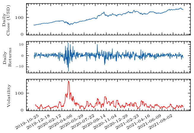
Figure 1: Apple’s daily data. The top row shows the price trend, the second row the associated daily returns, and the bottom row shows a volatility estimation calculated from a 5-days moving window over the daily returns.

3 Baseline Models and Metrics

3.1 Baseline Models

Most of the models commonly used for volatility forecasting can be traced back to Autoregressive Conditional Heteroscedastic (ARCH) models (Engle 1982). This family of models assume volatility clustering (Cont 2007), i.e., large shocks in prices tend to cluster together. ARCH-based models evolved into the well-known Generalized Autoregressive Conditional Heteroscedastic (GARCH) model (Bollerslev 1986), which is still widely utilised among industry participants. A GARCH$(p,q)$ process is given by:

$$\sigma_{t}^{2}=\omega+\sum_{i=1}^{p}\alpha_{i}\varepsilon_{t-i}^{2}+\sum_{j=1}^{q}\beta_{j}\sigma_{t-j}^{2},$$ (3)

where $\omega$ is the model’s bias, $q$ is the number of lags (order) of the observed volatility, $\sigma_{t}^{2}$; and $p$ is the number of lags of the innovations, $\varepsilon_{t}$. In turn, the returns of prices are related to the innovations by:

$$r_{t}=\mu+\varepsilon_{t},$$ (4)

where $\mu$ is the expected return (usually set to zero), and the volatility is related to these innovations by means of the residuals, $e_{t}$:

$$\varepsilon_{t}=\sigma_{t}e_{t},\quad e_{t}\sim\mathcal{N}(0,1).$$ (5)

The model’s parameters $\{\mu,\omega,\alpha,\beta\}$ can be estimated by performing maximum-likelihood estimation of the joint distribution $f\left(\varepsilon_{1},\ldots,\varepsilon_{T};\{\mu,\omega,\alpha,\beta\}\right)$. The simplest GARCH model consists on a GARCH$(1,1)$ process where $\sigma_{t}=1$ and $\mu=0$. Several variations leading to new architectures to address the volatility forecasting problem have been developed from the GARCH model. Here, we select some of them for benchmarking purposes. The integrated GARCH (IGARCH) model (Engle and Bollerslev 1986), modifies the design of the previous model to grant a longer memory in the autocorrelation of the squared returns, allowing the model to react in a more persistent way to the impact of past squared shocks. Also, IGARCH imposes the following restriction on the model’s parameters:

$$\sum_{i=1}^{p}\alpha_{i}+\sum_{j=1}^{q}\beta_{j}=1,$$ (6)

which makes the resulting process a weakly stationary one, since the mean, variance, and autocovariance are finite and constant over time. The idea behind the IGARCH model motivated the development of the Fractionally Integrated GARCH (FIGARCH) process (Baillie, Bollerslev, and Mikkelsen 1996), which is able to capture long-term volatility persistence and clustering features. To do so, it integrates a fractional difference operator (lag operator) $L$ into the conditional variance:

$$\sigma_{t}^{2}=\omega+\left[1-\beta L-\phi L(1-L)^{d}\right]\varepsilon_{t}^{2}+\beta\sigma_{t}^{2},$$ (7)

where $0<d<1$ is known as the fractional differencing parameters. The FIGARCH model has been widely used thanks to its ability to capture the volatility’s persistence and integrate it into its predictions (Cochran, Mansur, and Odusami 2012; Biage 2019). Threshold ARCH (TARCH) models (Rabemananjara and Zakoian 1993) are also used for benchmarking purposes. The main difference with respect to previous methodologies is that TARCH models divide the distribution of the innovations into disjoint intervals, which are later approximated by a linear function on the conditional standard deviation (Zakoian 1994). TARCH models are therefore capable of separately considering the influence of positive and negative innovations:

$$\sigma_{t}^{2}=\omega+\sum_{i=1}^{p}\alpha_{i}\varepsilon_{t-i}^{2}+\sum_{j=1}^{q}\beta_{j}\varepsilon_{t-j}^{2}\mathbb{I}_{\varepsilon_{t-j}<0},$$ (8)

where $\mathbb{I}_{(\cdot)}$ is the indicator function. The main characteristic of TARCH and other threshold-based approaches, such as TGARCH (Park, Baek, and Hwang 2009), is their ability to detect abrupt disruptions in the time-series through the indicator function, which may be replaced with a continuous function if a smoother transition is desired.

Volatility usually exhibits asymmetric characteristics. This property has led to the development of different asymmetric ARCH type models. For example, the Asymmetric Power ARCH (APARCH) model (Ding, Granger, and Engle 1993) assumes a parametric form for the conditional heteroskedasticity’s powers. It defines the variance dynamics as follows:

$$\sigma_{t}^{\delta}=\omega+\sum_{i=1}^{q}\alpha_{i}\left(\left|\varepsilon_{t-i}\right|-\gamma_{i}\varepsilon_{t-i}\right)^{\delta}+\sum_{j=1}^{p}\beta_{j}\sigma_{t-j}^{\delta},$$ (9)

where we now also have to estimate $\delta>0$, and $\gamma$. APARCH models nest many other volatility frameworks that can be obtained by imposing restrictions on the APARCH model’s parameters. A similar idea leads to the Asymmetric GARCH model (AGARCH) (Engle and Ng 1993), which captures the asymmetry in the volatility by using an impact curve associated with the $\alpha_{i}$ parameter:

$$\sigma_{t}^{2}=\omega+\sum_{i=1}^{p}\alpha_{i}\left(\varepsilon_{t-i}-\gamma_{i}\right)^{2}+\sum_{j=1}^{q}\beta_{j}\sigma_{t-j}^{2}.$$ (10)

Most of the mentioned models, like IGARCH or APARCH, impose restrictions on the parameters in practice, as Eq. (6) states. These restrictions are lifted in the Exponential GARCH (EGARCH) model (Nelson 1991), which is defined as:

$$\ln\sigma_{t}^{2}=\omega+\sum_{i=1}^{p}\alpha_{i}\left(\left|\epsilon_{t-i}\right|+\gamma_{i}\epsilon_{t-i}\right)+\sum_{j=1}^{q}\beta_{j}\ln\sigma_{t-j}^{2}.$$ (11)

As evidenced by the definition above, the EGARCH model integrates one powerful volatility clustering assumption into its architecture: negative shocks at time $t-1$ produce a stronger impact on the value of the volatility at time $t$ than positive shocks do, allowing for asymmetric effects between positive and negative asset returns. This asymmetry is known in the volatility forecasting literature as leverage effect (Bouchaud, Matacz, and Potters 2001).

All the methods described previously operate through the usage of daily returns. However, as mentioned above, more recent proposals have included the usage of realised measures obtained from the high-frequency data as additional input features for daily volatility forecasting. Among these methodologies, the High-Frequency-Based Volatility (HEAVY) model (Shephard and Sheppard 2010), has shown superior forecasting capabilities (Shephard and Sheppard 2010; Noureldin, Shephard, and Sheppard 2012; Sheppard and Xu 2019). Formally, the model is defined as follows:

$$\operatorname{var}\left(r_{t}\mid\mathcal{F}_{t-1}^{\mathrm{HF}}\right) =\sigma_{t}^{2}=\omega+\alpha\mathrm{RM}_{t-1}+\beta\sigma_{t-1}^{2},$$ (12)

$$\mathbb{E}\left(\mathrm{RM}_{t}\mid\mathcal{F}_{t-1}^{\mathrm{HF}}\right) =\mu_{t}=\omega_{R}+\alpha_{R}\mathrm{RM}_{t-1}+\beta_{R}\mu_{t-1},$$

where $r_{t}$ denotes daily returns, $RM_{t}$ denotes daily realised measures, and $\mathcal{F}_{t-1}^{\mathrm{HF}}$ denotes the high-frequency data utilised to obtain these realised measures. In previous equation, the restrictions $\{\omega,\alpha\geq 0,\beta\in[0,1)\}$ are imposed on the variation of the returns, and $\{\omega_{R},\alpha_{R},\beta_{R}\geq 0,\alpha_{R}+\beta_{R}\in[0,1)\}$ on the realised measures’ evolution, while observing the following variables:

$$\begin{array}[]{l}r_{t}=\sqrt{\sigma_{t}^{2}z_{t}},\\[4.26773pt] x_{t}=\mu_{t}z_{RV,t}^{2},\end{array}$$ (13)

with:

$$\left(\begin{array}[]{c}z_{t}\\ z_{RV,t}\end{array}\right)\sim\mathcal{N}(0,I).$$ (14)

Equation (12) shows that HEAVY consists of two parts. While $\sigma_{t}^{2}$ explains the development of the unobserved conditional variance, $\mu_{t}$ is responsible for explaining the development of the realised measures. The HEAVY model is clearly motivated by GARCH methodologies, which makes it simple to understand while reporting additional gains in the performance. For further details about it, like parameters inference, we refer the readers to (Shephard and Sheppard 2010).

3.2 Evaluation Metrics

In this section, we define a series of metrics that will be used to assess the day-ahead volatility forecast of our proposed architecture against previously defined baseline models. The Mean Absolute Error (MAE) and the Root Mean Squared Error (RMSE) constitute two of the most common error functions to evaluate the performance of volatility forecasting architectures. While a number of articles focus entirely on those two metrics to report performance (Shen, Wan, and Leatham 2021; Izzeldin et al. 2019), we complement them with the usage of the Symmetric Mean Absolute Percentage Error (SMAPE). This relative error measure has both a lower and upper bound, contrary to the Mean Absolute Percentage Error (MAPE), and it is scale independent. Also, the Maximum Error (ME) is used to illustrate which models produce the more significant inaccuracies: poor performance adapting to new regimes, as volatility shocks, lead certain models to substantial momentary discrepancies between the forecast and the actual volatility, which leads to an increase in the ME. We complement the ME with the Median Absolute Error (MedAE), an outliers-robust metric. Lastly, we include the Quasi Log-Likelihood (QLIKE), which has proven to be a noise robust loss function in the volatility proxy. Both the QLIKE and the RMSE will be used as loss functions to optimise the model’s parameters during Section 5, while the rest of the metrics will be used to assess the models’ performance. We summarise the definitions of all metrics below.

$$\ell_{\operatorname{\it{MAE}}}({\sigma}_{t}^{2},\hat{\sigma}_{t}^{2})=\frac{1}{T}\sum_{t=1}^{T}\left|{\sigma}_{t}^{2}-\hat{\sigma}_{t}^{2}\right|, \ell_{\operatorname{\it{rmse}}}({\sigma}_{t}^{2},\hat{\sigma}_{t}^{2})=\sqrt{\frac{1}{T}\sum_{t=1}^{T}\left({\sigma}_{t}^{2}-\hat{\sigma}_{t}^{2}\right)^{2}},$$ (15)

$$\ell_{\operatorname{\it{SMAPE}}}({\sigma}_{t}^{2},\hat{\sigma}_{t}^{2})=\frac{1}{T}\sum_{t=1}^{T}\frac{\left|{\sigma}_{t}^{2}-\hat{\sigma}_{t}^{2}\right|}{({\sigma}_{t}^{2}-\hat{\sigma}_{t}^{2})/2}, \ell_{\operatorname{\it{ME}}}({\sigma}_{t}^{2},\hat{\sigma}_{t}^{2})=\text{\it{max}}\left(\left|{\sigma}_{t}^{2}-\hat{\sigma}_{t}^{2}\right|\right),$$

$$\!\!\!\!\ell_{\operatorname{\it{MedAE}}}({\sigma}_{t}^{2},\hat{\sigma}_{t}^{2})=\text{\it{median}}(\sum_{t=1}^{T}\left|{\sigma}_{t}^{2}-\hat{\sigma}_{t}^{2}\right|), \!\!\ell_{\operatorname{\it{QLIKE}}}({\sigma}_{t}^{2},\hat{\sigma}_{t}^{2})=\frac{1}{T}\sum_{t=1}^{T}\log\left(\hat{\sigma}_{t}^{2}\right)+\frac{\sigma_{t}^{2}}{\hat{\sigma}_{t}^{2}},$$

where $\hat{\sigma}_{t}^{2}$ and ${\sigma}_{t}^{2}$ represent the volatility forecast and the volatility proxy measure, respectively, with $T$ the total amount of rolling forecasts.

4 Model

4.1 Problem Definition

Considering a set of assets, $\Delta\in\mathbb{R}^{d}$, where $d\in\mathbb{N}$ denotes the dimension of the input vector, with $T\in\mathbb{N}$ days’ intraday high-frequency data associated to them, $\{\mathbf{r}_{t}^{1:J}\}_{t=1}^{T}$, where $\mathbf{r}_{t}^{1:J}=(r_{t}^{1},r_{t}^{2},\ldots,r_{t}^{J})$ are the intraday returns of the $t$-th day, with $T$ being referred to as receptive field, and with ${J\in\mathbb{N}}$ the length of each day’s intraday data, our goal is to forecast the day-ahead realised volatility:

$$\hat{\sigma}^{2}_{T+1}=f_{\theta}\left(r_{t=1}^{1},r_{t=1}^{2},\ldots,r_{t=1}^{J},r_{t=2}^{1},\ldots,r_{t=T}^{1},\ldots,r_{t=T}^{J}\right),$$ (16)

where $f_{\theta}:\mathbb{R}^{d}\rightarrow\mathbb{R}^{m},m\in\mathbb{N},$ is a function implemented through a Dilated Causal Convolutions (DCC)-based neural network, with $\theta\in\Theta$ being the learnable parameters of the model from a set $\Theta\in\mathbb{R}^{n}$, for some $n\in\mathbb{N}$.

These parameters fully specify the corresponding volatility forecast. Therefore, we aim to obtain the set of optimal parameters $\hat{\theta}\in\Theta$ that minimises the difference between the forecasted volatility, $\hat{\sigma}_{t}^{2}$, and the volatility’s proxy measure ${\sigma}_{t}^{2}$ for the considered assets:

$$\hat{\theta}=\underset{\theta\in\Theta}{\operatorname{argmin}}\,\mathcal{L}\left(f_{\theta}(\Delta),{\sigma}_{t}^{2}(\Delta)\right),$$ (17)

where $\mathcal{L}$ is the selected metric for evaluating the forecast accuracy.

4.2 Dilated Causal Convolutions

Our volatility forecasting proposal, DeepVol, uses DCCs as a technique to integrate the high-frequency information into the realised volatility prediction. The deployment of such an architecture allows the usage of a large receptive field, permiting an increase in the size of the input sequences while preserving the number of parameters of the network, yielding improved computational efficiency. The proposed architecture consists of $L$ convolutional layers. The convolution operation performed by the first layer, between the input sequences $x$ and the kernel $k$, can be defined as follows:

$$F^{(l=1)}(t)=\left(x*_{d}k^{(l=1)}\right)(t)=\sum_{\tau=0}^{s-1}k^{(l=1)}_{\tau}\cdot x_{t-d\tau},$$ (18)

being $d$ the dilation factor and $k$ the filter, with size $s\in\mathbb{Z}$. For each of the rest $l$-th layers, we can define the convolution operation as:

$$F^{(l)}(t)=\left(F^{(l-1)}*_{d}k^{(l)}\right)(t)=\sum_{\tau=0}^{s-1}k^{(l)}_{\tau}\cdot F_{t-d\tau}^{l-1}(t).$$ (19)

As previous equations state, the inner product performed by the dilated causal convolutions is based on entries that are a fixed number of steps apart from each other, contrary to CNN and Causal-CNN, which operate with consecutive entries. Furthermore, each of the layers in this hierarchical structure defines the kernel operation as an affine function acting between layers:

$$k^{(l)}:\mathbb{R}^{N_{l}}\longrightarrow\mathbb{R}^{N_{l+1}},1\leq l\leq L.$$ (20)

As previous equations show, through the usage of residual connections, firstly proposed in He et al. (2016), the model connects $l$-th layer’s output to $(l+1)$-th layer’s input, enabling the usage of deeper models with larger receptive fields. The complete operative of the proposed model can be defined as follows:

$$\sigma^{2}_{T+1}(\{\mathbf{r}_{t}^{1:J}\}_{t=1}^{T})=\alpha_{0}+\sum_{l=1}^{L}\alpha_{l}\,\sigma_{ReLu}(F^{(l)}(\{\mathbf{r}_{t}^{1:J}\}_{t=1}^{T})),$$ (21)

where $\sigma_{ReLu}:\mathbb{R}\mapsto\mathbb{R}$ is the selected non-linearity and $\{\alpha_{0},\cdots,\alpha_{l},\cdots,\alpha_{L}\}$ is a set of weights applied to the convolutional operations. Figure 2 presents an overview of the utilised architecture, where a receptive field with previous $T$ days’ intraday data is processed through a hierarchy of dilated convolutions to forecast the day-ahead realised volatility.

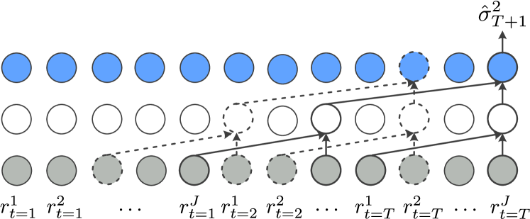
Figure 2: DeepVol intrinsic architecture. The dilation factor grows exponentially, allowing an increase in the receptive field without increasing the model’s complexity.

DeepVol, like any deep-feed-forward neural network, is approximating the volatility’s unknown function through sample pairs of input and output data $(x,y)$. Formally speaking, DeepVol is approximating some function $f_{\theta}(\cdot)$ which is not available in closed form by finding the optimal model’s parameters $\hat{\theta}$ derived from the best function approximation $f^{*}_{\theta}(\cdot)$.

5 Experiments

In this section, DeepVol’s volatility forecasts will be evaluated and compared with the baseline models described in Section 3.1. For benchmarking purposes, we will utilise the metrics described in Section 3.2. Besides classic out-of-sample forecast comparisons, we perform different experiments to present some additional insights into the inner workings of DeepVol. We analyse DeepVol’s behaviour while varying the intraday data sampling frequency, studying the discrepancy in model behaviour when trained on different granularity regimes. In close relation to this, we also explore the usage of different receptive field sizes and how this affects the model performance. Finally, we analyse the inclusion of realised measures as an extra input to the model, studying if its addition can improve the forecasting accuracy. Besides the models presented in Section 3.1, we also include a martingale process for comparison purposes.

5.1 Experiments Setup

We apply the same architecture to all the experiments in this section, using the Quasi Log-Likelihood as loss function to train the model parameters. We choose Adaptive Moment Estimation Algorithm (ADAM) (Kingma and Ba 2014) as optimiser, even though different experiments were conducted exploring the usage of Averaged Stochastic Gradient Descent (ASGD) (Kingma and Ba 2014) and Limited Memory BFGS (L-BFGS) (Liu and Nocedal 1989). While the usage of these optimisers usually entails smoother predictions, the reported performance declined with respect to ADAM, hence, they were not considered further. Early stopping is used during the training process. DeepVol is implemented in Pytorch-Lightning (Falcon and The PyTorch Lightning team 2019), and the experiments are conducted using a NVIDIA Titan Xp GPU.

5.2 Out-of-sample Forecast

This section aims to provide an out-of-sample performance comparison between the proposed model and some classical methodologies widely used in the finance industry. For this purpose, we use the NASDAQ-100 dataset described in Section 2.1, which is split into two folds. The first of them contains the intraday data from September 30, 2019, to December 31, 2020. The second fold includes data from January 1, 2021, to September 30, 2021. The 15 months of data of the first fold will be used for training purposes, while the remaining nine months will be used to evaluate the out-of-sample performance of the models. For this specific study, a sampling frequency of 5 minutes for the intraday data and a receptive field of one day (using $t$-day intraday’s data to predict the realised volatility for day $t+1$) are utilised.

Table 1: Out-of-sample forecast: experiments results for the NASDAQ-100 dataset.

Method		MAE	RMSE	SMAPE	QLIKE	ME	MedAE
martingale		5.180	11.410	0.324	747.480	96.654	1.614
TARCH		4.849	10.320	0.301	351.310	71.659	2.804
IGARCH		5.008	10.534	0.302	351.702	72.048	2.797
FIGARCH		4.631	10.356	0.294	349.245	71.050	2.460
APARCH		4.730	10.096	0.299	349.974	70.088	2.859
AGARCH		4.833	10.304	0.324	351.217	71.215	2.819
EGARCH		4.793	10.180	0.300	348.614	70.615	2.917
HEAVY		4.565	10.239	0.292	343.490	72.404	2.545
DeepVol		3.903	8.457	0.279	340.779	71.779	2.008

Table 1 summarises the out-of-sample forecast performance of the different models we evaluated. It can be seen that the proposed architecture, DeepVol, improves the baseline results for most metrics, with the exception of ME and MedAE. Peculiarly, for the later, the martingale process proves to provide the best results. Considering that the MadAE is an outlier-robust error function, this behaviour is not surprising, as the martingale process is the most conservative among the evaluated strategies. For this particular error metric, DeepVol is the second-best in performance terms.

As mentioned before, the evaluated baseline methodologies operate in a recurrent manner, utilising all available past data, while DeepVol uses just the previous day’s intraday information for the day-ahead prediction. Considering these facts, DeepVol’s good performance with respect to the MedAE is especially surprising, as noisier behaviour could be expected due to the lack of recurrence. Furthermore, some of the baseline models evaluated, as the HEAVY model, integrate momentum indicators into their architecture, something that we do not explicitly model in DeepVol. Consequently, DeepVol’s accurate predictions in terms of MAE and RMSE are particularly interesting considering how the model maintains a low MedAE. In conclusion, the proposed architecture shows robustness in the presence of volatility shocks and avoids an escalation on the ME and MedAE as unstable methods would report.

Table 2 extends the results of Table 1, displaying the improvement/degradation for each evaluated method relative to a basic martingale process and the HEAVY model. For the former, we aim to report how much improvement each model provides over the most basic modelling of the problem. For the latter, considering that the HEAVY model is the best performer among the baselines architectures, a direct comparison with it is especially useful for analysing DeepVol’s performance.

Table 2: Out-of-sample forecast: percentage of improvement/degradation over the martingale process and the HEAVY model, for each of the evaluated models.

Method		MAE	RMSE	SMAPE	QLIKE	ME	MedAE
		Improvement over martingale (%)
martingale		-	-	-	-	-	-
TARCH		6.398	9.553	7.099	53.001	25.860	-73.730
IGARCH		3.320	7.677	6.790	52.948	25.458	-73.296
FIGARCH		10.598	9.238	9.259	53.277	26.490	-52.410
APARCH		8.687	11.516	7.716	53.179	27.486	-77.138
AGARCH		6.699	9.693	0.000	53.013	26.319	-74.659
EGARCH		7.471	10.780	7.407	53.361	26.940	-80.731
HEAVY		11.873	10.263	9.877	54.047	25.089	-57.677
DeepVol		24.653	25.881	13.889	54.410	25.736	-24.411
		Improvement over HEAVY (%)
martingale		-13.472	-11.437	-10.959	-117.613	-33.492	36.579
TARCH		-6.212	-0.791	-3.082	-2.277	1.029	-10.181
IGARCH		-9.704	-2.881	-3.425	-2.391	0.492	-9.906
FIGARCH		-1.446	-1.143	-0.685	-1.675	1.870	3.340
APARCH		-3.614	1.397	-2.397	-1.888	3.120	-12.342
AGARCH		-5.871	-0.635	-10.959	-2.250	1.642	-10.771
EGARCH		-4.995	0.576	-2.740	-1.492	2.471	-14.621
HEAVY		-	-	-	-	-	-
DeepVol		14.502	17.404	4.452	0.789	0.863	21.097

DeepVol thoroughly overperforms HEAVY concerning the MAE, RMSE, SMAPE, and MedAE errors, while the differences in QLIKE and ME are tighter. As previously mentioned, we consider particularly interesting DeepVol’ ability to overperform the rest of the models while proving a robust noise behaviour, avoiding an escalation in the ME and MedAE while performing more accurate predictions.

5.3 Receptive Field and Sampling Frequency Analysis

The receptive field size and the intraday sampling frequency are two model parameters which shed light on the inner workings of DeepVol when analysed further. Therefore, its analysis is particularly interesting in order to understand the model’s behaviour. As mentioned in Section 2.2, a number of studies have validated the optimal intraday data sampling frequency for computation of the realised measures from high-frequency data (Andersen, Bollerslev, and Meddahi 2006; Hansen and Lunde 2006; Corradi and Distaso 2006), commonly concluding that using a granularity of 5 or 10 minutes minimises the microstructure noise effect while maximising the usage of high-frequency information. In this section, we study this same trade-off in the proposed deep-learning architecture, analysing the effect that using different sampling frequencies has on model performance.

Furthermore, increasing the receptive field size is a practical way of extending the network’s capabilities without modifying its architecture or increasing its complexity. For example, while DeepVol could be easily modified to integrate a momentum indicator, increasing its receptive field should entail a similar effect, providing DeepVol with the possibility of incorporating past data if it is informative enough for the realised volatility forecasting.

Table 3: Receptive field and sampling frequency study.

Sampling Frequency	Receptive Field		MAE	RMSE	SMAPE	QLIKE	ME	MedAE
1 min	1		4.096	8.462	0.287	342.313	71.749	2.396
5 min	1		3.903	8.457	0.279	340.779	71.779	2.008
	2		4.429	9.495	0.308	367.209	70.036	1.756
	3		4.054	8.379	0.285	343.359	70.457	2.334
15 min	1		3.993	8.436	0.283	343.412	70.915	2.185
	2		4.651	10.437	0.312	365.893	70.926	1.836
	3		5.817	9.520	0.323	362.235	72.338	4.577
	5		6.736	10.217	0.336	366.192	72.240	5.594
30 min	1		4.259	9.699	0.318	689.633	75.793	1.632
	2		4.503	10.140	0.327	789.326	79.345	1.724
	3		4.473	9.931	0.324	784.843	75.059	1.705
	5		4.705	10.802	0.326	833.966	83.416	1.676
	10		4.732	11.084	0.327	853.981	85.656	1.591
60 min	1		4.988	10.516	0.297	366.509	82.207	2.402
	2		5.616	12.596	0.324	709.082	99.828	2.178
	3		5.441	12.615	0.319	688.996	99.612	2.017
	5		5.520	12.456	0.326	714.871	95.763	2.071
	10		4.997	11.186	0.322	706.917	87.096	1.927

Table 3 collects the results of an analysis whose main objective is to evaluate if DeepVol’s performance is robust to increasing the receptive field or modifying the sampling frequency. It is interesting to note that using intraday data from one day with a sampling frequency of 5-minutes proves to be optimal. This scenario reports the best results with regard to all the considered metrics but the MedAE. Secondly, the increment of the receptive field leads to a degradation of performance. This indicates that, for the proposed architecture, all the relevant information for forecasting the day-ahead volatility can be obtained from the previous day high-frequency data. Otherwise, the model yields more conservative predictions that degrade its performance. Thirdly, the best performance in terms of MedAE is obtained when using a 30 minutes sampling frequency, together with a receptive field of ten days. This result can be directly related to the hypothesis previously mentioned: A longer receptive field leads to a more conservative forecast, resulting in a lower Median Absolute Error. In this scenario, the model is less prone to forecast volatility jumps, a behaviour commonly associated with integrating momentum indicators. However, this specific setup leads to a deterioration in all the other metrics. The growth in the receptive field size prevents the model from forecasting more drastic changes in the presence of volatility shocks, leading to more conservative predictions than the ones reported when using just the previous day intraday data.

5.4 Linearity Study

Table 4: Linearity Study. DeepVol + RV merges DeepVol’s predictions with the realised variance through a linear layer and additional non-linearities.

	Receptive Field		MAE	RMSE	SMAPE	QLIKE	ME	MedAE
DeepVol + RV	1		4.130	8.720	0.286	345.150	72.292	2.193
	2		6.804	10.036	0.335	369.529	69.309	5.728
	3		6.899	10.008	0.340	371.762	69.903	6.577
DeepVol	1		3.903	8.457	0.279	340.779	71.779	2.008
	2		4.429	9.495	0.308	592.600	78.690	1.756
	3		4.054	8.379	0.285	343.359	70.457	2.334

The analyses of the previous sections have shown that the usage of a receptive field of one day and a sampling frequency of 5-minutes reports the most accurate results for forecasting the day-ahead realised volatility. In addition, we wanted to study possible gains of including realised measures into our methodology. The intuition behind this idea is that integrating previous days’ realised measures information as an extra input would allow DeepVol to observe a bigger window of past data, allowing the model to complement high-frequency data with extra historical information of the time-series.

To integrate the realised measures into DeepVol, we slightly modify its architecture, adding a linear output as a final layer. This last layer merged the results of the dilated convolutions performed over the high-frequency data with the realised measures, each of them weighted by its corresponding terms. Different receptive fields were validated while integrating the realised measures. The reported results are shown in Table 4, where it can be noted that our DNNs-based proposal does not benefit from the inclusion of realised measures as an extra input feature. Adding the past realised measures results in an analogous behaviour to increasing the receptive field, highlighting again that DeepVol is especially efficient in utilising recent high-frequency data for volatility forecasting, not requiring a more extended lookback window to do so.

5.5 Generalisation and Transfer Learning Analysis

Previous experiments used all NASDAQ-100 tickers during training and testing, preserving a portion of the dataset’s dates for the out-of-sample forecast. In this section, in addition, we split the dataset into two folds in the cross-section. During training, just half of the tickers are used, while the other half is utilised for testing. For training purposes, we use the first four months of data corresponding to the first half of tickers, that is, from September 30, 2019, through January 30, 2020. The model is later tested on the remainder tickers, using data from February 01, 2020, through September 30, 2021. This set-up allows us to evaluate the quality of the models’ forecasts during the volatility shocks provoked by the COVID-19 crisis, which started in February, 2020. This scenario allows us to evaluate our model’s generalisation capabilities, predicting the day-ahead volatility for tickers that were not previously available. As done in Section 5.5, a 5-minutes sampling frequency and a receptive field of one day are used. The results of this out-of-sample-stocks forecast study are collected in Table 5. In these conditions, DeepVol still report the best MAE, RMSE, and SMAPE results, while the HEAVY model reports a better QLIKE than the rest of the evaluated methods. Concerning the MeadAE, DeepVol reports the best results, immediately followed by the martingale process, which still outperforms the rest of the baseline models. These results, which are similar to the obtained in the out-of-sample forecast study of Section 5.5, confirm that DeepVol still shows a conservative behaviour in this new forecast scenario, proving its generalisation capabilities to transfer learning from training to test, learning global features of the data that allow the model to perform well on out-of-distribution data. As in Section 5.5, Table 6 reports the improvement/degradation for each evaluated method with respect to a basic martingale process and the HEAVY model on the test set tickers.

Table 5: Out-of-sample-stocks forecast. Generalisation Study: experiments results for the NASDAQ-100 dataset.

Method		MAE	RMSE	SMAPE	QLIKE	ME	MedAE
martingale		9.673	35.235	0.324	2142.795	341.457	2.169
TARCH		8.525	28.178	0.295	893.795	282.096	3.236
IGARCH		9.208	27.753	0.312	947.409	279.080	3.982
FIGARCH		7.805	26.752	0.299	899.955	267.533	3.581
APARCH		8.179	26.749	0.297	896.063	265.910	3.557
AGARCH		7.928	26.486	0.294	893.682	269.577	3.191
EGARCH		8.180	26.767	0.297	897.432	277.022	3.530
HEAVY		8.315	26.322	0.294	874.409	277.780	2.158
DeepVol		7.288	23.396	0.292	894.283	275.255	1.927

Table 6: Out-of-sample-stocks forecast: percentage of improvement/degradation over the martingale process and the HEAVY model. for each of the evaluated models.

Method		MAE	RMSE	SMAPE	QLIKE	ME	MedAE
		Improvement over martingale (%)
martingale		-	-	-	-	-	-
TARCH		11.863	20.030	9.068	58.288	17.385	-49.161
IGARCH		4.804	21.235	3.671	55.786	18.268	-83.565
FIGARCH		19.315	24.075	7.711	58.001	21.650	-65.089
APARCH		15.440	24.083	8.267	58.183	22.125	-63.973
AGARCH		18.043	24.829	9.251	58.294	21.051	-47.105
EGARCH		15.443	24.032	8.452	58.119	18.871	-62.737
HEAVY		14.037	25.295	9.200	59.193	18.649	0.534
DeepVol		24.660	33.599	9.932	58.266	19.388	11.165
		Improvement over HEAVY (%)
martingale		-16.330	-33.859	-10.132	-145.056	-22.924	-0.537
TARCH		-2.529	-7.048	-0.145	-2.217	-1.554	-49.962
IGARCH		-10.741	-5.434	-6.090	-8.349	-0.468	-84.551
FIGARCH		6.140	-1.632	-1.640	-2.921	3.689	-65.975
APARCH		1.632	-1.622	-1.028	-2.476	4.273	-64.854
AGARCH		4.660	-0.623	0.056	-2.204	2.953	-47.895
EGARCH		1.624	-1.691	-0.824	-2.633	0.273	-63.611
HEAVY		-	-	-	-	-	-
DeepVol		12.357	11.116	0.806	-2.273	0.909	10.688

Finally, Figures 3 to 6 show different examples on how the evaluated models generalise and transfer learning from the train tickers into the test distribution. Model forecasts are shown together with the daily squared returns, allowing a direct comparison between forecasts from DeepVol and baselines. Note that classical methodologies return smoother predictions, a phenomenon especially visible in the HEAVY model as it integrates a momentum indicator. This behaviour, associated with more conservative predictions, clearly poses a disadvantage in terms of slower adaptation to volatility shocks. Several of these volatility shocks, provoked by the COVID-19 crisis in 2020 and 2021, are easily recognisable in the associated figures. All the evaluated models reacted to the bigger of these shocks, the 2020 stock market crash, starting in February 2020, in one way or another. Otherwise, during the minor shocks that followed that year, baseline predictions are almost negligible with the exception of IGARCH in Fig. 6. HEAVY and EGARCH exhibit an invariable behaviour in this turbulent environment, showing a lack of adaptability to changing conditions. We should remark that DeepVol requires just one day of intraday data to perform the out-of-sample volatility forecasting, unlike classical methodologies which operate recursively, forcing them to use a sufficiently long window of past data. This places DeepVol in an advantaged position in situations of low data availability, such as the inclusion of new tickers in the stock market, as it does not require a long horizon of historical to perform its predictions.

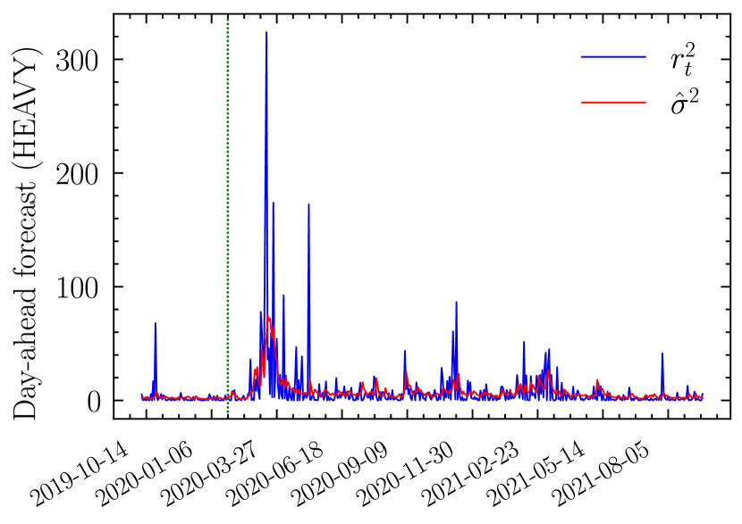
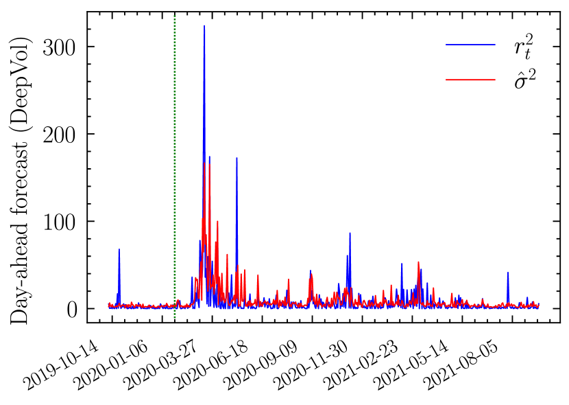
Figure 3: Out-of-sample-stocks: HEAVY’s and DeepVol’s forecast on PYPL. Green dotted vertical lines mark the forecast start.

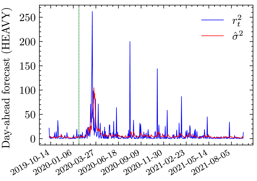
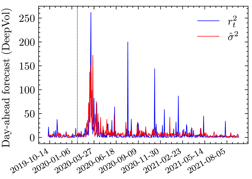
Figure 4: Out-of-sample-stocks: HEAVY’s and DeepVol’s forecast on QCOM. Green dotted vertical lines mark the forecast start.

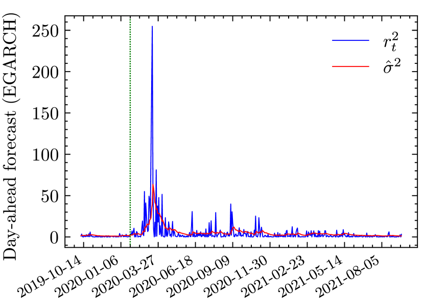
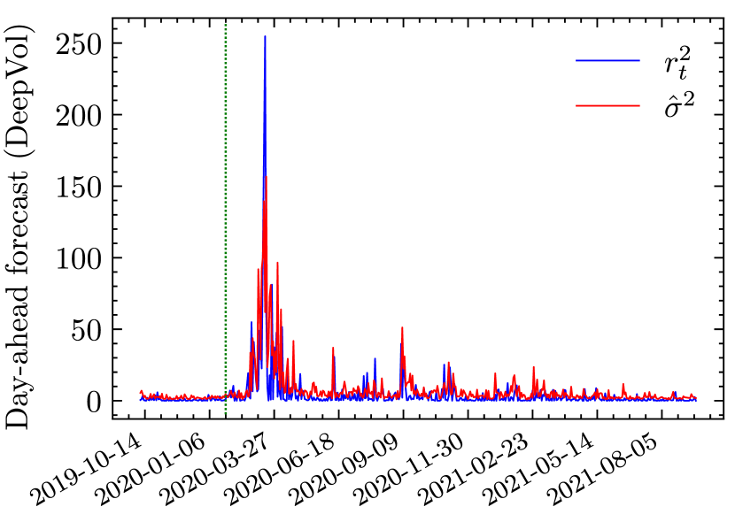
Figure 5: Out-of-sample-stocks: EGARCH’s and DeepVol’s forecast on MSFT. Green dotted vertical lines mark the forecast start.

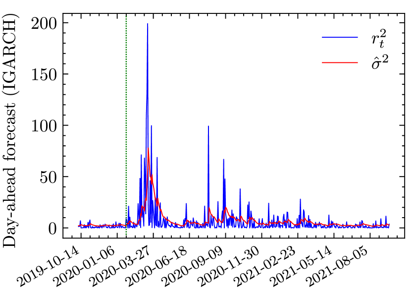
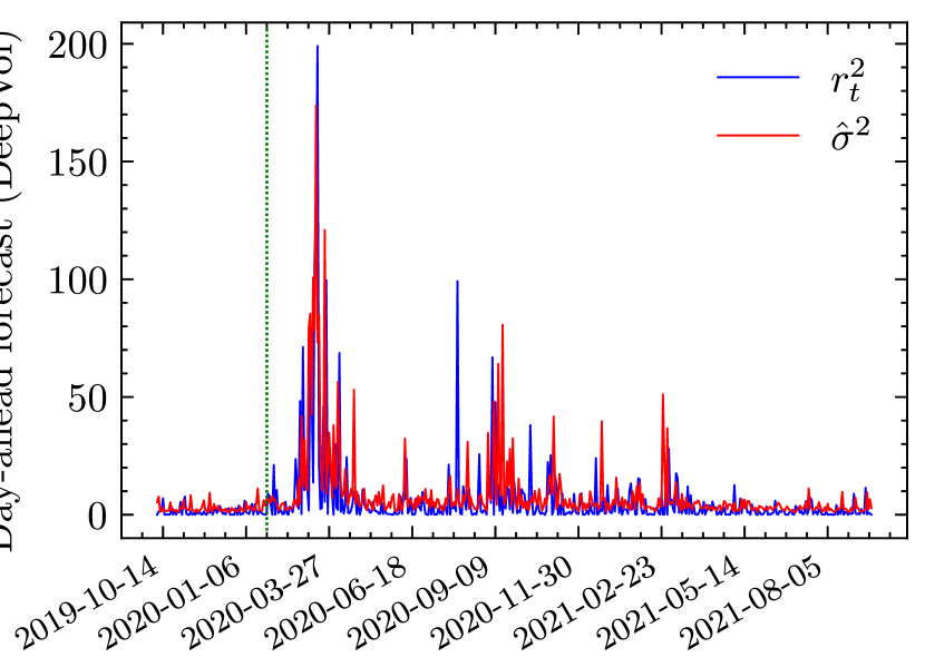
Figure 6: Out-of-sample-stocks: IGARCH’s and DeepVol’s forecast on AAPL. Green dotted vertical lines mark the forecast start.

5.6 Discussion of Results

Several findings from the experiments are worth highlighting with regard to the usage of Dilated Causal Convolutions for the day-ahead realised volatility forecasting. Firstly, DeepVol generally outperforms traditional autoregressive architectures, showing a quicker adaptation to volatility shocks while maintaining some conservatism in its predictions, as the reported MedAE and ME in previous experiments shows. Specifically, DeepVol’s reported accuracy seems particularly interesting considering that the experiments were conducted in high volatility regimes. The reported results resemble extensive literature indicating that deep-learning-based volatility forecasting architectures (Ramos-Pérez, Alonso-González, and Núñez-Velázquez 2021) and hybrid models (Baek and Kim 2018; Kim and Won 2018) consistently outperform classical methodologies.

Experiments in Section 5.3 have highlighted that, for the proposed method, data from the previous trading day contains enough information for predicting the day-ahead realised volatility with high accuracy. Furthermore, a sampling frequency of 5-minutes has shown to maximise the trade-off between noise and intraday information, echoing studies analysing this same trade-off in the context of estimation of realised measures from high-frequency data. Finally, DeepVol consistently outperforms baseline methods while reporting good results in outlier-robust metrics such as MedAE, proving that the model quickly adapts to volatility shocks while demonstrating noise robustness.

6 Conclusions

In this paper, we propose a deep learning model based on hierarchies of Dilated Causal Convolutions – termed DeepVol – to forecast day-ahead realised volatility from high-frequency data. Our model takes advantage of the automatic feature extraction inherent to Deep Neural Networks to bypass the estimation of the realised measures, tackling the problem of volatility forecasting from a pure data-driven perspective. At the same time, the usage of dilated convolutions enables DeepVol to exponentially increase its input window, performing a similar operation to how handcrafted realised measures condense high-frequency information. Reported results show how DeepVol’s predictions significantly improve the baseline models performance, proving that the proposed data-driven approach avoids the limitations of classical methods, such as model misspecification or the usage of hand-crafted noisy realised measures, by taking advantage of the abundance of high-frequency data.

The proposed architecture outperforms baseline methods while exhibiting robustness in the presence of volatility shocks, avoiding an increases in Maximum and Median Absolute Errors, as reported by other unstable methods. Those results are especially relevant considering that experiments were conducted in high volatility regimes, such as the 2020 stock crisis caused by the COVID-19 pandemic. In context of the generalisation study, where out-of-sample-stocks forecasts are conducted, DeepVol shows its ability to extract universal features and transfer learning to out-of-distribution data. Additionally, we observe that for DeepVol the previous day intraday data makes the most significant contribution to predict the day-ahead volatility. Therefore, increasing the receptive field of DeepVol does not generally lead to better performance. Moreover, we show that using a 5-minutes sampling frequency optimises the trade-off between maximising the usage of high-frequency data information while minimising the microstructure noise implicit to higher sampling frequencies. This result is particularly interesting as it reminiscent of earlier studies validating this same trade-off for the construction of realised measures. The empirical results collected in this paper suggest that models based on Dilated Causal Convolutions should be carefully considered in the context of volatility forecasting and as a result can play a key role in the valuation of financial derivatives, risk management, and portfolio construction.

References

- Ait-Sahalia, Mykland, and Zhang (2005) Ait-Sahalia, Yacine, Per A Mykland, and Lan Zhang. 2005. “How often to sample a continuous-time process in the presence of market microstructure noise.” The review of financial studies 18 (2): 351–416.
- Andersen, Bollerslev, and Meddahi (2006) Andersen, TG, Tim Bollerslev, and Nour Meddahi. 2006. “Market microstructure noise and realized volatility forecasting.” Unpublished paper: Department of Economics, Duke University .
- Andersen, Bollerslev, and Diebold (2010) Andersen, Torben G, Tim Bollerslev, and Francis X Diebold. 2010. “Parametric and nonparametric volatility measurement.” In Handbook of financial econometrics: Tools and techniques, 67–137. Elsevier.
- Andersen et al. (2001) Andersen, Torben G, Tim Bollerslev, Francis X Diebold, and Heiko Ebens. 2001. “The distribution of realized stock return volatility.” Journal of financial economics 61 (1): 43–76.
- Baars (2014) Baars, Bjorn. 2014. HEAVY and Realized (E) GARCH Models. GlobeEdit.
- Baek and Kim (2018) Baek, Yujin, and Ha Young Kim. 2018. “ModAugNet: A new forecasting framework for stock market index value with an overfitting prevention LSTM module and a prediction LSTM module.” Expert Systems with Applications 113: 457–480.
- Bahdanau, Cho, and Bengio (2014) Bahdanau, Dzmitry, Kyunghyun Cho, and Yoshua Bengio. 2014. “Neural machine translation by jointly learning to align and translate.” arXiv preprint arXiv:1409.0473 .
- Baillie, Bollerslev, and Mikkelsen (1996) Baillie, Richard T, Tim Bollerslev, and Hans Ole Mikkelsen. 1996. “Fractionally integrated generalized autoregressive conditional heteroskedasticity.” Journal of econometrics 74 (1): 3–30.
- Bandi and Russell (2006) Bandi, Federico M, and Jeffrey R Russell. 2006. “Separating microstructure noise from volatility.” Journal of Financial Economics 79 (3): 655–692.
- Biage (2019) Biage, Milton. 2019. “Analysis of shares frequency components on daily value-at-risk in emerging and developed markets.” Physica A: Statistical Mechanics and its Applications 532: 121798.
- Bollerslev (1986) Bollerslev, Tim. 1986. “Generalized autoregressive conditional heteroskedasticity.” Journal of econometrics 31 (3): 307–327.
- Borovykh, Bohte, and Oosterlee (2017) Borovykh, Anastasia, Sander Bohte, and Cornelis W Oosterlee. 2017. “Conditional time series forecasting with convolutional neural networks.” arXiv preprint arXiv:1703.04691 .
- Bouchaud, Matacz, and Potters (2001) Bouchaud, Jean-Philippe, Andrew Matacz, and Marc Potters. 2001. “Leverage effect in financial markets: The retarded volatility model.” Physical review letters 87 (22): 228701.
- Brownlees and Gallo (2010) Brownlees, Christian T, and Giampiero M Gallo. 2010. “Comparison of volatility measures: a risk management perspective.” Journal of Financial Econometrics 8 (1): 29–56.
- Chen and Robert (2021) Chen, Qinkai, and Christian-Yann Robert. 2021. “Multivariate Realized Volatility Forecasting with Graph Neural Network.” arXiv preprint arXiv:2112.09015 .
- Cochran, Mansur, and Odusami (2012) Cochran, Steven J, Iqbal Mansur, and Babatunde Odusami. 2012. “Volatility persistence in metal returns: A FIGARCH approach.” Journal of Economics and Business 64 (4): 287–305.
- Cont (2007) Cont, Rama. 2007. “Volatility clustering in financial markets: empirical facts and agent-based models.” In Long memory in economics, 289–309. Springer.
- Corradi and Distaso (2006) Corradi, Valentina, and Walter Distaso. 2006. “Semi-parametric comparison of stochastic volatility models using realized measures.” The Review of Economic Studies 73 (3): 635–667.
- Corsi (2009) Corsi, Fulvio. 2009. “A simple approximate long-memory model of realized volatility.” Journal of Financial Econometrics 7 (2): 174–196.
- Ding, Granger, and Engle (1993) Ding, Zhuanxin, Clive WJ Granger, and Robert F Engle. 1993. “A long memory property of stock market returns and a new model.” Journal of empirical finance 1 (1): 83–106.
- Engle (1982) Engle, Robert F. 1982. “Autoregressive conditional heteroscedasticity with estimates of the variance of United Kingdom inflation.” Econometrica: Journal of the econometric society 987–1007.
- Engle and Bollerslev (1986) Engle, Robert F, and Tim Bollerslev. 1986. “Modelling the persistence of conditional variances.” Econometric reviews 5 (1): 1–50.
- Engle and Ng (1993) Engle, Robert F, and Victor K Ng. 1993. “Measuring and testing the impact of news on volatility.” The journal of finance 48 (5): 1749–1778.
- Falcon and The PyTorch Lightning team (2019) Falcon, William, and The PyTorch Lightning team. 2019. “PyTorch Lightning.” 3. https://github.com/Lightning-AI/lightning.
- Hansen and Lunde (2006) Hansen, Peter R, and Asger Lunde. 2006. “Realized variance and market microstructure noise.” Journal of Business & Economic Statistics 24 (2): 127–161.
- Hansen, Huang, and Shek (2012) Hansen, Peter Reinhard, Zhuo Huang, and Howard Howan Shek. 2012. “Realized GARCH: a joint model for returns and realized measures of volatility.” Journal of Applied Econometrics 27 (6): 877–906.
- Harvey et al. (2018) Harvey, Campbell R, Edward Hoyle, Russell Korgaonkar, Sandy Rattray, Matthew Sargaison, and Otto Van Hemert. 2018. “The impact of volatility targeting.” The Journal of Portfolio Management 45 (1): 14–33.
- He et al. (2016) He, Kaiming, Xiangyu Zhang, Shaoqing Ren, and Jian Sun. 2016. “Deep residual learning for image recognition.” In Proceedings of the IEEE conference on computer vision and pattern recognition, 770–778.
- Hochreiter and Schmidhuber (1997) Hochreiter, Sepp, and Jürgen Schmidhuber. 1997. “Long short-term memory.” Neural computation 9 (8): 1735–1780.
- Horvath, Muguruza, and Tomas (2019) Horvath, Blanka, Aitor Muguruza, and Mehdi Tomas. 2019. “Deep learning volatility.” arXiv preprint arXiv:1901.09647 .
- Izzeldin et al. (2019) Izzeldin, Marwan, M Kabir Hassan, Vasileios Pappas, and Mike Tsionas. 2019. “Forecasting realised volatility using ARFIMA and HAR models.” Quantitative Finance 19 (10): 1627–1638.
- Karanasos, Yfanti, and Hunter (2022) Karanasos, Menelaos, Stavroula Yfanti, and John Hunter. 2022. “Emerging stock market volatility and economic fundamentals: the importance of US uncertainty spillovers, financial and health crises.” Annals of operations research 313 (2): 1077–1116.
- Kim and Won (2018) Kim, Ha Young, and Chang Hyun Won. 2018. “Forecasting the volatility of stock price index: A hybrid model integrating LSTM with multiple GARCH-type models.” Expert Systems with Applications 103: 25–37.
- Kingma and Ba (2014) Kingma, Diederik P, and Jimmy Ba. 2014. “Adam: A method for stochastic optimization.” arXiv preprint arXiv:1412.6980 .
- Labys et al. (1999) Labys, Paul, Torben Andersen, Tim Bollerslev, and Francis X Diebold. 1999. The distribution of exchange rate volatility. National Bureau of Economic Research.
- Li et al. (2019) Li, Shiyang, Xiaoyong Jin, Yao Xuan, Xiyou Zhou, Wenhu Chen, Yu-Xiang Wang, and Xifeng Yan. 2019. “Enhancing the locality and breaking the memory bottleneck of transformer on time series forecasting.” Advances in neural information processing systems 32.
- Lim and Zohren (2021) Lim, Bryan, and Stefan Zohren. 2021. “Time-series forecasting with deep learning: a survey.” Philosophical Transactions of the Royal Society A 379 (2194): 20200209.
- Lin et al. (2022) Lin, Yu, Zixiao Lin, Ying Liao, Yizhuo Li, Jiali Xu, and Yan Yan. 2022. “Forecasting the realized volatility of stock price index: A hybrid model integrating CEEMDAN and LSTM.” Expert Systems with Applications 117736.
- Liu and Nocedal (1989) Liu, DC, and J Nocedal. 1989. “On the limited memory method for large scale optimization: Mathematical Programming B.” .
- Mademlis and Dritsakis (2021) Mademlis, Dimitrios Kartsonakis, and Nikolaos Dritsakis. 2021. “Volatility Forecasting using Hybrid GARCH Neural Network Models: The Case of the Italian Stock Market.” International Journal of Economics and Financial Issues 11 (1): 49.
- Moreira and Muir (2017) Moreira, Alan, and Tyler Muir. 2017. “Volatility-managed portfolios.” The Journal of Finance 72 (4): 1611–1644.
- Moreno-Pino, Olmos, and Artés-Rodríguez (2021) Moreno-Pino, Fernando, Pablo M Olmos, and Antonio Artés-Rodríguez. 2021. “Deep autoregressive models with spectral attention.” arXiv preprint arXiv:2107.05984 .
- Nelson (1991) Nelson, Daniel B. 1991. “Conditional heteroskedasticity in asset returns: A new approach.” Econometrica: Journal of the econometric society 347–370.
- Noureldin, Shephard, and Sheppard (2012) Noureldin, Diaa, Neil Shephard, and Kevin Sheppard. 2012. “Multivariate high-frequency-based volatility (HEAVY) models.” Journal of Applied Econometrics 27 (6): 907–933.
- Oord et al. (2016) Oord, Aaron van den, Sander Dieleman, Heiga Zen, Karen Simonyan, Oriol Vinyals, Alex Graves, Nal Kalchbrenner, Andrew Senior, and Koray Kavukcuoglu. 2016. “Wavenet: A generative model for raw audio.” arXiv preprint arXiv:1609.03499 .
- Papantonis, Rompolis, and Tzavalis (2022) Papantonis, Ioannis, Leonidas Rompolis, and Elias Tzavalis. 2022. “Improving variance forecasts: The role of Realized Variance features.” International Journal of Forecasting .
- Park, Baek, and Hwang (2009) Park, JA, JS Baek, and SY Hwang. 2009. “Persistent-threshold-GARCH processes: Model and application.” Statistics & Probability Letters 79 (7): 907–914.
- Rabemananjara and Zakoian (1993) Rabemananjara, Roger, and Jean-Michel Zakoian. 1993. “Threshold ARCH models and asymmetries in volatility.” Journal of applied econometrics 8 (1): 31–49.
- Rahimikia and Poon (2020) Rahimikia, Eghbal, and Ser-Huang Poon. 2020. “Big data approach to realised volatility forecasting using HAR model augmented with limit order book and news.” Available at SSRN 3684040.
- Rahimikia, Zohren, and Poon (2021) Rahimikia, Eghbal, Stefan Zohren, and Ser-Huang Poon. 2021. “Realised Volatility Forecasting: Machine Learning via Financial Word Embedding.” arXiv preprint arXiv:2108.00480 .
- Ramos-Pérez, Alonso-González, and Núñez-Velázquez (2021) Ramos-Pérez, Eduardo, Pablo J Alonso-González, and José Javier Núñez-Velázquez. 2021. “Multi-transformer: A new neural network-based architecture for forecasting S&P volatility.” Mathematics 9 (15): 1794.
- Reisenhofer, Bayer, and Hautsch (2022) Reisenhofer, Rafael, Xandro Bayer, and Nikolaus Hautsch. 2022. “HARNet: A convolutional neural network for realized volatility forecasting.” arXiv preprint arXiv:2205.07719 .
- Rumelhart, Hinton, and Williams (1985) Rumelhart, David E, Geoffrey E Hinton, and Ronald J Williams. 1985. Learning internal representations by error propagation. Technical Report. California Univ San Diego La Jolla Inst for Cognitive Science.
- Shen, Wan, and Leatham (2021) Shen, Ze, Qing Wan, and David J Leatham. 2021. “Bitcoin Return Volatility Forecasting: A Comparative Study between GARCH and RNN.” Journal of Risk and Financial Management 14 (7): 337.
- Shephard and Sheppard (2010) Shephard, Neil, and Kevin Sheppard. 2010. “Realising the future: forecasting with high-frequency-based volatility (HEAVY) models.” Journal of Applied Econometrics 25 (2): 197–231.
- Sheppard and Xu (2019) Sheppard, Kevin, and Wen Xu. 2019. “Factor high-frequency-based volatility (HEAVY) models.” Journal of Financial Econometrics 17 (1): 33–65.
- Su (2021) Su, Jung-Bin. 2021. “How to promote the performance of parametric volatility forecasts in the stock market? a neural networks approach.” Entropy 23 (9): 1151.
- Van Oord, Kalchbrenner, and Kavukcuoglu (2016) Van Oord, Aaron, Nal Kalchbrenner, and Koray Kavukcuoglu. 2016. “Pixel recurrent neural networks.” In International conference on machine learning, 1747–1756. PMLR.
- Vaswani et al. (2017) Vaswani, Ashish, Noam Shazeer, Niki Parmar, Jakob Uszkoreit, Llion Jones, Aidan N Gomez, Łukasz Kaiser, and Illia Polosukhin. 2017. “Attention is all you need.” Advances in neural information processing systems 30.
- Vidal and Kristjanpoller (2020) Vidal, Andrés, and Werner Kristjanpoller. 2020. “Gold volatility prediction using a CNN-LSTM approach.” Expert Systems with Applications 157: 113481.
- Yu and Li (2018) Yu, ShuiLing, and Zhe Li. 2018. “Forecasting stock price index volatility with LSTM deep neural network.” In Recent developments in data science and business analytics, 265–272. Springer.
- Yuan, Li, and Wang (2022) Yuan, Huiling, Guodong Li, and Junhui Wang. 2022. “High-Frequency-Based Volatility Model with Network Structure.” arXiv preprint arXiv:2204.12933 .
- Zakoian (1994) Zakoian, Jean-Michel. 1994. “Threshold heteroskedastic models.” Journal of Economic Dynamics and control 18 (5): 931–955.