LTH/1315

October 2022

Spectroscopy in the 2+1$d$ Thirring Model with $N=1$ Domain Wall Fermions

Simon Hands and Johann Ostmeyer

Department of Mathematical Sciences, University of Liverpool,

Liverpool L69 3BX, U.K.

Abstract

We employ the domain wall fermion (DWF) formulation of the Thirring model on a lattice in 2+1+1 dimensions and perform $N=1$ flavor Monte Carlo simulations. At a critical interaction strength the model features a spontaneous $\mathrm{U}(2)\rightarrow\mathrm{U}(1)\otimes\mathrm{U}(1)$ symmetry breaking; we analyse the induced spin-0 mesons, both Goldstone and non-Goldstone, as well as the correlator of the fermion quasiparticles, in both resulting phases. Crucially, we determine the anomalous dimension $\eta_{\psi}\approx 3$ at the critical point, in stark contrast with the Gross-Neveu model in 3$d$ and with results obtained with staggered fermions. Our numerical simulations are complemented by an analytical treatment of the free fermion correlator, which exhibits large early-time artifacts due to branch cuts in the propagator stemming from unbound interactions of the fermion with its heavy doublers. These artifacts are generalisable beyond the Thirring model, being an intrinsic property of DWF, or more generally Ginsparg-Wilson fermions.

Keywords: four-fermi, Monte Carlo simulation, dynamical fermions, spontaneous symmetry breaking, anomalous dimension

1 Introduction

The Thirring model is a quantum field theory of reducible (ie. 4-component) fermions interacting via a current-current contact term, specified in three dimensional continuum Euclidean spacetime by the following Lagrangian:

$${\cal L}=\bar{\psi}_{i}(\partial{\!\!\!/}\,+m)\psi_{i}+{g^{2}\over{2N}}(\bar{\psi}_{i}\gamma_{\mu}\psi_{i})^{2},$$ (1)

with $i=1,\ldots,N$ indexing flavor degrees of freedom. While (1) can be used to model electron dynamics in layered systems found in condensed matter physics, it is theoretically interesting in its own right due to its potential for exhibiting a UV-stable renormalisation group fixed point where a strongly-interacting continuum quantum field theory may be defined. Since there is no small parameter in play, large anomalous scaling dimensions are anticipated, so that the resulting theory will almost certainly lie in a new universality class characterised by non-canonical critical exponents, a scenario referred to as a Quantum Critical Point (QCP). This possibility may be explored by several means; here we continue a programme of lattice field theory simulations in which the QCP is identified in the $m\to 0$ limit with a transition in which the formation of a bilinear condensate $\langle\bar{\psi}\psi\rangle$ spontaneously breaks the model’s global U(2$N$) symmetry leading to the dynamical generation of a fermion mass. Further background can be found in recent reviews [1, 2].

The U(2$N$) symmetry of (1) is explicitly broken to U($N$)$\otimes$U($N$) in the presence of a fermion mass $m\not=0$. Neither Wilson (with no symmetry protecting against gap formation) nor staggered (where the breaking is instead U($N)\otimes$U($N)\to$U($N$)) lattice fermion formulations faithfully represent this pattern of breaking symmetry, which is problematic when the QCP dynamics are strong and there is no means to control the recovery of symmetry analytically. Our approach utilises domain wall fermions (DWF); on a finite system with domain walls separated by $L_{s}$ in a direction $x_{3}$, there is accumulated evidence both analytically and numerically that U(2$N$) is recovered in the limit $L_{s}\to\infty$ [3, 4, 5, 6]. Studies of the Thirring model with $N=1$ have revealed evidence for a QCP described by an empirical equation of state for the order parameter $\langle\bar{\psi}\psi(m,g)\rangle$ corresponding to critical exponents with non-mean field values [6, 7], and distinct from those obtained from simulations of the model formulated with staggered lattice fermions [8]. Moreover, simulations with $N=2$ have failed to identify a condensate for $m\to 0$, consistent with a critical flavor number $1<N_{c}<2$, with $N\leq N_{c}$ needed for the QCP’s existence [9], and again in disparity with the $N_{c}\approx 7$ observed for staggered fermions [10].

In this paper we turn our attention to two-point functions, studying both fermion – antifermion “meson” bound states in the spin-0 channel, and also the propagating fermion “quasiparticle” in the spin-${1\over 2}$ channel. The calculations employ orthodox lattice field theory techniques, and for a massive theory, which we can ensure by setting $m\not=0$, yield information on the particle spectrum. Since the quasiparticle propagator is not gauge-invariant in a gauge theory, to our knowledge this is the first time elementary fermion excitations have been studied using DWF. In principle it will enable us to distinguish broken from symmetric phases via dynamical fermion mass generation and the appearance of Goldstone bosons whose mass has a characteristic dependence on $m$ in the former case. However, the DWF setup also enables a study of the massless $m=0$ limit, in which case exactly at the critical point $g=g_{c}$ all correlations are expected to decay algebraically, with a power sensitive to the critical dynamics. Study of the quasiparticle propagator now furnishes information on a critical exponent $\eta_{\psi}$, defined via $\langle\psi(x)\bar{\psi}(0)\rangle\sim x^{-(2+\eta_{\psi})}$, an important characteristic of the QCP not accessed via the equation of state, which focusses on the scalar order parameter field.

The rest of the paper is organised as follows. In Sec. 2 we recall the lattice formulation of the Thirring model (1) with DWF, and define the correlation functions to be calculated in terms of fields $\Psi,\bar{\Psi}$ defined on a 2+1+1$d$ lattice. Since the study of elementary fermion propagators is new, analytic insight is welcome; in Sec. 3 we have attempted to collect results for the free fermion propagator which will inform studies in both this and future work, including a simple analytic model which to good accuracy reproduces a numerically significant artifact resulting from a branch cut in the exact form (29) below. It is demonstrated that finite-$L_{s}$ artifacts are reduced if instead of $m\bar{\psi}\psi$ the U($2N$)-equivalent mass term $im\bar{\psi}\gamma_{3}\psi$ is used, corroborating earlier studies of the condensate $\langle\bar{\psi}\psi\rangle$ [3, 4, 5]. Dependence on the domain wall height $M$ is also studied. Sec. 4 presents spectrum results from numerical simulations on a $16^{2}\times 48\times L_{s}$ system with varying $m,g$ and the domain wall separations $L_{s}=64,80$ used in the most recent equation-of-state study [7]. Our fitting procedure is described in detail; we study 3 distinct spin-0 mesons including both Goldstone and non-Goldstone channels (a non-Goldstone requiring the evaluation of disconnected diagrams is omitted for now) and the fermion quasiparticle. In Sec. 5 we turn our attention to the fermion channel with $m$ set to zero. First we develop continuum models for the quasiparticle propagator at a QCP, ie. with anomalous dimension $\eta_{\psi}\not=0$, showing that in general a UV regularisation is required. We also present an Ansatz for how the propagator might be modified away from the QCP in the symmetric phase, ie. with a finite correlation length $\mu^{-1}$ where $\mu$ is not a pole mass. Finally we present numerical results taken at 5 different couplings in the symmetric phase including one very close to the QCP deduced from equation of state studies [7], obtaining an estimate $\eta_{\psi}\approx 3$ at the critical point. Sec. 6 discusses our results, with some technical details postponed to the Appendices A, B and C.

2 Lattice Formulation and Methodology

The lattice model studied here is the “bulk” variant of the formulation first set out in [5], employing domain wall fermions (DWF) in 2+1+1$d$:

$$S=S_{\rm kin}+S_{\rm int}+S_{\rm aux}=\sum_{x,y}\sum_{s,s^{\prime}}\bar{\Psi}(x,s){\cal M}_{x,s;y,s^{\prime}}\Psi(y,s^{\prime})+S_{\rm aux}.$$ (2)

Here $\Psi,\bar{\Psi}$ are 4-spinors defined on a hypercubic lattice with 2+1$d$ indices $x$ and an index $s$ labelling the “third” direction $x_{3}$, taking values $s=1,\ldots,L_{s}$. Free fermions are described by the kinetic operator

$${\cal M}_{0}=\delta_{s,s^{\prime}}D_{Wx,y}+\delta_{x,y}D_{3s,s^{\prime}}+mS_{m3};$$ (3)

$D_{W}$ is the 2+1$d$ Wilson operator with domain wall height $M$:

$$D_{W}(M)_{x,y}=-{1\over 2}\sum_{\mu=0,1,2}[(1-\gamma_{\mu})\delta_{x+\hat{\mu},y}+(1+\gamma_{\mu})\delta_{x-\hat{\mu},y}]+(3-M)\delta_{x,y}.$$ (4)

Throughout this work we use $M=1$. Hopping along $x_{3}$ is governed by

$$D_{3}(L_{s})_{s,s^{\prime}}=-[P_{-}\delta_{s+1,s^{\prime}}(1-\delta_{s,L_{s}})+P_{+}\delta_{s-1,s^{\prime}}(1-\delta_{s,1})]+\delta_{s,s^{\prime}}.$$ (5)

The factors $(1-\delta_{s,1/L_{s}})$ implement open boundary conditions at domain walls located at $s=1,L_{s}$, while the projectors $P_{\pm}={1\over 2}(1\pm\gamma_{3})$ also appear in the definition of the target physical fermion degrees of freedom $\psi,\bar{\psi}$ defined on the walls:

$$\psi(x)\equiv P_{-}\Psi(x,1)+P_{+}\Psi(x,L_{s});\;\;\;\bar{\psi}(x)\equiv\bar{\Psi}(x,L_{s})P_{-}+\bar{\Psi}(x,1)P_{+}.$$ (6)

Finally, the mass term is defined in terms of fields on the walls via

$$mS_{m3}=im\sum_{x}\bar{\psi}(x)\gamma_{3}\psi(x).$$ (7)

This form of the mass term yields superior convergence to the U(2)-symmetric limit anticipated as $L_{s}\to\infty$ over the conventional $m\bar{\psi}\psi$  [3, 5].

The interaction term is between a fermion current and a real non-compact vector field $A_{\mu}$ defined on the links of the spacetime lattice:

$$S_{\rm int} = {i\over 2}\sum_{x,\mu,s}A_{\mu}(x)\left[\bar{\Psi}(x,s)(-1+\gamma_{\mu})\Psi(x+\hat{\mu},s)+\bar{\Psi}(x+\hat{\mu},s)(1+\gamma_{\mu})\Psi(x,s)\right]$$ (8)

$$\equiv \sum_{x,\mu}A_{\mu}(x){\cal J}_{\mu}(x)$$

Integration over the auxiliary field specified by the Gaussian action

$$S_{\rm aux}={1\over{2g^{2}}}\sum_{x,\mu}A_{\mu}^{2}(x),$$ (9)

results in a four-fermion contact interaction $-{g^{2}\over 2}{\cal J}_{\mu}{\cal J}_{\mu}$ between conserved non-local currents

$${\cal J_{\mu}}(x)=\sum_{s=1}^{L_{s}}j_{\mu}(x,s);\;\;\;\Delta^{-}_{\mu}{\cal J}_{\mu}(x)=\sum_{s}\Delta_{\mu}^{-}j_{\mu}(x,s)=0.$$ (10)

with the local current ($\nu\in\{\mu,3\}$)

$$j_{\nu}(x,s)={i\over 2}\left[\bar{\Psi}(x,s)(\gamma_{\nu}-1)\Psi(x+\hat{\nu},s)+\bar{\Psi}(x+\hat{\nu},s)(\gamma_{\nu}+1)\Psi(x,s)\right]$$ (11)

obeying a 2+1$d$ continuity equation (Cf. [12]):

$$\Delta_{\mu}^{-}j_{\mu}(x,s)=\begin{cases}-j_{3}(x,1)-m\bar{\psi}(x)\psi(x)&s=1\\ -\Delta_{3}^{-}j_{3}(x,s)&1<s<L_{s}\\ +j_{3}(x,L_{s}-1)+m\bar{\psi}(x)\psi(x)&s=L_{s}.\end{cases}$$ (12)

The fermion matrix ${\cal M}[A_{\mu}]$ superficially resembles that of an abelian gauge theory, with link fields $e^{\pm iA_{\mu}}$ replaced by non-unitary links $(1\pm iA_{\mu})$. At strong coupling this non-unitary nature presents challenges, both in inverting ${\cal M}$ and in the recovery of U(2) as $L_{s}\to\infty$ [6]. In practice $N=1$ dynamics are simulated with an RHMC algorithm based on the positive measure $\mbox{det}({\cal M}^{\dagger}{\cal M})^{1\over 2}$; details can be found in [9, 6] and the simulation code is available at [13].

Quasiparticle and meson propagators are calculated in terms of the 2+1+1$d$ propagator $S(m;x,s;y,s^{\prime})=\langle\Psi(x,s)\bar{\Psi}(y,s^{\prime})\rangle$, which obeys two useful identities [3]:

$$\gamma_{5}S(m;x,s;y,s^{\prime})\gamma_{5} = S^{\dagger}(m;y,s^{\prime};x,s);$$ (13)

$$\gamma_{3}S(m;x,s;y,s^{\prime})\gamma_{3} = S^{\dagger}(-m;y,\bar{s}^{\prime};x,\bar{s}),$$ (14)

with $\bar{s}\equiv L_{s}-s+1$. Meson propagators in spin-0 channels are then defined using local bilinear sources via

$$C_{\Gamma}(x)=\langle\bar{\psi}(0)\Gamma\psi(0)\bar{\psi}(x)\Gamma\psi(x)\rangle;\;\;\;\Gamma\in\{\gamma_{3},\gamma_{5},1\kern-4.5pt1,\gamma_{3}\gamma_{5}\}.$$ (15)

Using the definition (6) and relations (13,14) they can all be expressed in terms of the primitive correlators [3, 9]

$$C^{--}(x) = \mbox{tr}[S(m;0,1;x,L_{s})P_{-}S^{\dagger}(m;0,1,x,L_{s})P_{-}];$$

$$C^{+-}(x) = \mbox{tr}[S(m;0,1;x,1)P_{+}S^{\dagger}(m;0,1,x,1)P_{-}];$$

$$\tilde{C}^{--}(x) = \mbox{tr}[S(m;0,1;x,L_{s})P_{-}S^{\dagger}(-m;0,1,x,L_{s})P_{-}];$$

$$\tilde{C}^{+-}(x) = \mbox{tr}[S(m;0,1;x,1)P_{+}S^{\dagger}(-m;0,1,x,L_{s})P_{-}],$$ (16)

requiring two inversions of ${\cal M}$ for each source location on the $s=1$ wall. The resulting expressions are

$$C_{\gamma_{5}}(x) \equiv C_{\rm G^{-}}(x) =|C^{--}(x)+C^{+-}(x)|;$$ (17)

$$C_{1\kern-4.5pt1}(x) \equiv C_{\rm G^{+}}(x) =|\tilde{C}^{--}(x)-\tilde{C}^{+-}(x)|;$$ (18)

$$C_{\gamma_{3}}(x) \equiv C_{\rm NG^{+}}(x) =|\tilde{C}^{--}(x)+\tilde{C}^{+-}(x)|;$$ (19)

$$C_{\gamma_{3}\gamma_{5}}(x) \equiv C_{\rm NG^{-}}(x) =|C^{--}(x)-C^{+-}(x)|.$$ (20)

The channel subscripts denote whether the meson is Goldstone or non-Goldstone, based on an anticipated U(2)$\to$U(1)$\otimes$U(1) symmetry breaking induced by a symmetry-breaking mass term $im\bar{\psi}\gamma_{3}\psi$. Parity $\pm$ assignments follow the definition

$$\psi(x)\overset{\cal P}{\mapsto}\gamma_{3}\psi(-x);\;\;\;\bar{\psi}(x)\overset{\cal P}{\mapsto}\bar{\psi}(-x)\gamma_{3}\,,$$ (21)

chosen to leave this mass term invariant. Note that in the case of symmetry breaking the NG⁺ channel also has a significant contribution of the opposite sign from disconnected fermion line diagrams, which we do not attempt to calculate.

In the spin-${1\over 2}$ sector the timeslice propagator for free fields is

$$S_{f}(x_{0})=\sum_{\vec{x}}\langle\psi(0)\bar{\psi}(x)\rangle\sim\int{dp_{0}\over 2\pi}{e^{ip_{0}x_{0}}\over{ip_{0}\gamma_{0}+im\gamma_{3}}}={{-i\gamma_{3}\pm\gamma_{0}}\over 2}e^{-m|x_{0}|},$$ (22)

where $\pm$ denotes the sign of the temporal displacement $x_{0}$. In terms of 2+1+1$d$ propagators this motivates the measurements

$$S_{0}(x_{0})={1\over 4}\mbox{tr}\gamma_{0}S_{f}(x_{0})\!\!\! = \!\!\!{1\over 4}\sum_{\vec{x}}\mbox{tr}\gamma_{0}[P_{-}S(m;0,1;x,1)+P_{+}S(m;0,L_{s};x,L_{s})];$$

$$S_{3}(x_{0})={i\over 4}\mbox{tr}\gamma_{3}S_{f}(x_{0})\!\!\! = \!\!\!{i\over 4}\sum_{\vec{x}}\mbox{tr}[-P_{-}S(m;0,1;x,L_{s})+P_{+}S(m;0,L_{s};x,1)].$$

For enhanced sampling expressions (LABEL:eq:quasiprop) are evaluated using a wall source; since there is no need for gauge-fixing, this presents no additional complications. We sampled every 5th trajectory, using sources located at 5 different timeslices, each requiring separate inversions on two distinct Dirac-indexed sources to evaluate (LABEL:eq:quasiprop). This was found to yield substantially improved results compared to earlier studies employing smeared sources [5].

3 Free Fermion Correlator

In this section we collect together some analytic results and approximations for the free fermion correlator using DWF, with the goal of understanding the discretisation effects introduced by the lattice as well as the influence of domain wall height $M$ and separation $L_{s}$. All the considered formulations have the correct continuum limit, but they approach it differently swiftly which can be crucial for simulations with limited computational resources. This will inform the numerical study of the fermion propagator in the interacting theory to be presented in Secs. 4,5.

We explicitly distinguish between the two mass operators $i\gamma_{3}m_{3}$ as in equation (7) and the conventional hermitian $m_{h}$ in this section. Since we are interested in analytic results here, we derive the free fermion propagator in terms of operators rather than the measured quantities $S(m;x,s;y,s^{\prime})$. Furthermore we work in momentum space. Following Ref. [5], we obtain the expressions (formally equivalent to those in equation (LABEL:eq:quasiprop))

$$C(p;1,1) =\operatorname{Tr}\left[\gamma_{0}P_{-}D^{\dagger}(p;1,s)G(p;s,1)\right]\,,$$ (24)

$$C(p;1,L_{s}) =\begin{cases}\operatorname{Tr}\left[P_{-}D^{\dagger}(p;1,s)G(p;s,L_{s})\right]\,,&m=m_{h}\\ \operatorname{Tr}\left[-i\gamma_{3}P_{-}D^{\dagger}(p;1,s)G(p;s,L_{s})\right]\,,&m=i\gamma_{3}m_{3}\end{cases}$$ (25)

where the Wilson operator $D$ (corresponding to $\cal M_{0}$ in (3)) and the Green function $G$ are defined by

$$D^{\dagger}(p;1,s) =\theta(s-1)\theta(L_{s}-s)\left[-P_{+}\delta_{s,2}+(b-i\not{\bar{p}})\delta_{s,1}+mP_{-}\delta_{s,L_{s}}\right]\,,$$ (26)

$$\begin{split}G(p;s,s^{\prime})&=\left(P_{+}A_{+}+P_{-}A_{-}\right)\mathrm{e}^{-\alpha(s+s^{\prime}-2)}+\left(P_{+}A_{-}+P_{-}A_{+}\right)\mathrm{e}^{-\alpha(2L_{s}-s-s^{\prime})}\\ &\quad+B\mathrm{e}^{-\alpha|s-s^{\prime}|}+A_{m}\left(\mathrm{e}^{-\alpha(L_{s}-s+s^{\prime}-1)}+\mathrm{e}^{-\alpha(L_{s}+s-s^{\prime}-1)}\right)\end{split}$$ (27)

respectively, with the auxiliary variables $\alpha,\bar{p},b,A_{\pm},A_{m}$, and $B$ listed in Section A.1.

For zero spatial momentum, the explicit evaluation of the traces in (24) and (25) yields the form

$$C(p=(p_{0},0,0)) =C((p_{0},0,0);1,1)+C((p_{0},0,0);1,L_{s})$$ (28)

$$=\frac{2im\sin(p_{0})+2\cos(p_{0})+\sqrt{5-4\cos(p_{0})}-1}{i\left(m^{2}+1\right)\sin(p_{0})+2m\cos(p_{0})-m}$$ (29)

in the large $L_{s}$ limit and setting the domain wall height $M=1$ immediately. The exact form for finite $L_{s}$ can be found in Appendix B.

We obtain the same expression for both mass terms, $i\gamma_{3}m_{3}$ and $m_{h}$, in the $L_{s}\rightarrow\infty$ limit as expected. The convergence in the $m_{3}$ case is significantly faster, however, as we will discuss later on.

3.1 The free propagator in momentum and real space

Often the physical intuition obtained from exact analytic calculations is rather limited. We will therefore investigate an approximation that captures all the important physics without ‘having too many trees to see the forest’.

We start out with the well known (up to a constant and irrelevant factor 2) free particle propagator in continuous space

$$C_{\rm cont}(p) =\frac{2}{m+ip}\,.$$ (30)

Going to a lattice, we have to substitute the momentum $p$ for the lattice momentum $\sin p$. The simplest realisation with the correct continuum limit is then

$$C_{\rm naive}(p) =\frac{2}{m+i\sin p}\,,$$ (31)

which, of course, leads to the infamous doubling problem since the $\sin$-function has zeros not only at integer multiples of $2\pi$, but also at multiples of $\pi$. The domain wall approach essentially gets rid of this problem by lifting the unphysical pole near $p=\pi$ (assuming $m\ll 1$). The exact formula (29) is a particular realisation of this requirement, and so is

$$C_{0}(p) =\frac{1+n(m)\cos p}{m+i\sin p}\,,\quad n(m)\coloneqq\frac{1}{\sqrt{1+m^{2}}}\,.$$ (32)

Figure 1 shows that $C$ and $C_{0}$ are quite compatible, so we are going to use the simplistic version $C_{0}(p)$ in further analysis.

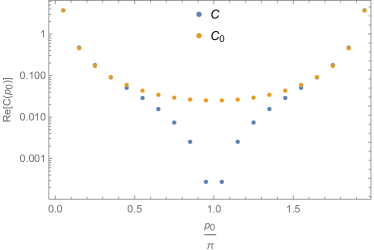
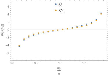
Figure 1: Exact and approximate free fermion propagators at zero spatial momentum in momentum space, $m=$0.05$$. Real part left, imaginary part right.

We are interested in the propagator in (imaginary) time, still at zero spatial momentum, so we have to perform a Fourier transformation

$$C_{0}(t) =\frac{1}{L_{t}}\sum_{p_{0}}C_{0}(p)\mathrm{e}^{ip_{0}t}\,,$$ (33)

where $p_{0}$ ranges over fermionic Matsubara modes. The full derivation of the exact form is provided in Section A.2 and it yields

$$C_{0}(t) =\frac{\mathrm{e}^{-\tilde{m}t}}{\mathrm{e}^{-\tilde{m}L_{t}}+1}\frac{2}{\sqrt{1+m^{2}}}-\delta_{t0}\,,$$ (34)

where $\tilde{m}\coloneqq\operatorname{sinh^{-1}}m$. In the zero temperature ($L_{t}\rightarrow\infty$) and continuum ($m\rightarrow 0$, but $mt=\text{const.}$) limits $C_{0}(t)$ approaches the expected form $\mathrm{e}^{-mt}$.

3.2 Leading order corrections

The propagator $C_{0}$ derived in Sec. 3.1 captures the important intermediate time $1\ll t\ll L_{t}$ features including some lattice artefacts and the absence of the doubler. There are, however, more subtle but still substantial discretisation effects not yet considered. When considering the exact form $C(p)$ instead of the simplified $C_{0}(p)$, the most prominent difference is that $C(p)$ has not only poles but also branch cuts due to the $\sqrt{5-4\cos p}$ term. The square root stems from the quadratic nature of $DD^{\dagger}$ solved for the Greens function [5], or more generally from the quadratic (chirality breaking) term of order $\operatorname{\mathcal{O}}\left(a\right)$ in the Ginsparg-Wilson equation [14]. While all the other differences are analytic and can therefore feature only in higher orders of $m$, this non-holomorphicity has an immediate impact on the contour integral and therefore on $C(t)$. The existence of branch cuts in the DWF representation has been noted before [15], but to the best of our knowledge so far neither their origins nor their implications have been investigated.

Branch cuts indicate unbound many-particle interactions [16], in this case between the fermion and its doubler. These interactions are very short ranged for heavy doublers and decouple completely in the continuum limit. Put differently, the branch cuts can only start at energies larger than the sum of fermion and doubler masses and therefore vanish in the limit of infinitely heavy doublers. Here we see again that DWF (or more generally Ginsparg-Wilson fermions) do not get rid of the doublers in principle, but rather assign zero weight to the single particle doubler poles.

Again, the details of the modified correlator’s derivation can be found in Section A.3. We call the modified propagator that incorporates both $C_{0}$ and the branch cuts

$$\tilde{C}_{0}(t) =C_{0}(t)+\sqrt{\frac{3}{4\pi}}\left(\frac{1}{m+\frac{3}{4}}\frac{2^{t-L_{t}}}{\left(L_{t}-t+\frac{3}{4}\right)^{3/2}}+\frac{1}{\frac{3}{4}-m}\frac{2^{-t}}{\left(t+\frac{3}{4}\right)^{3/2}}\right)$$ (35)

and we show all three propagators as a function of $t$ in figure 2. As expected the unphysical contributions vanish exponentially fast when $t$ and $L_{t}-t$ are large, so that the correct results are obtained in the continuum and zero temperature limits. Careful zooming in reveals some small differences between $C$ and $\tilde{C}_{0}$ at the edges of the diagram, but the leading order features are described very well.

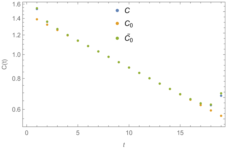
Figure 2: Exact and approximate free fermion propagators at zero spatial momentum in real space, $m=$0.05$$.

3.3 Influences of the Domain wall height and separation

Throughout this work we set the DW height $M=1$ and therefore do not go into detail about its influence on the propagator here. A short summary of how $M$ affects the propagator is provided in Appendix B.

More importantly, the DW separation $L_{s}$ has to be chosen finite in actual simulations so that the $L_{s}\rightarrow\infty$ limit assumed in this section so far is not always justified. We show the behaviour of the propagators at small domain wall separations in figure 3. $C_{h}$ (i.e. using $m=m_{h}$) exhibits significant deviations from the case discussed above for $L\lesssim 6$, whereas $C_{3}$ (i.e. using $m=i\gamma_{3}m_{3}$) remains virtually unchanged until $L\lesssim 3$. We find that both expressions contain first order $\mathrm{e}^{-\alpha L_{s}}$-terms but $C_{3}$ has only imaginary and order $\operatorname{\mathcal{O}}\left(m\right)$ suppressed contributions, resulting in smaller finite $L_{s}$ effects. See Appendix B for the exact formulae.

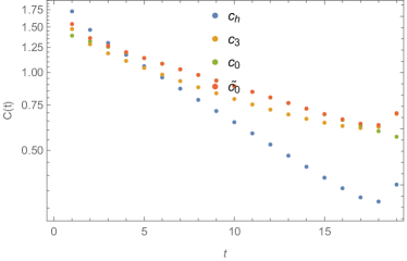
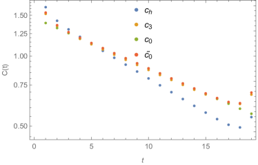
Figure 3: Exact and approximate free fermion propagators at zero spatial momentum in real space, bare mass $m=$0.05$$, domain wall separations top: $L_{3}=3$, $L_{s}=4$; bottom: $L_{s}=5$, $L_{s}=6$.

Let us stress at this point that the finite $L_{s}$ effects are significantly larger in the interacting case (Cf. the results for the equation of state presented in [6, 7]) and one cannot choose the DW separation from these free theory calculations. We can nevertheless infer that $C_{3}$ approaches the physical $L_{s}\rightarrow\infty$ limit faster than $C_{h}$ justifying our use of this particular formulation throughout this work.

In summary, the results of this section demonstrate that while DWF introduce new forms of short-distance artifact due to a branch cut not present in traditional lattice formulations, the results are in perfect accord with the free fermions in the continuum $am\to 0$ and low temperature $L_{t}\to\infty$ limits. These insights will aid interpretation of the numerical results for interacting fermions to follow in Secs. 4,5.

4 Results from $16^{2}\times 48$

In this section we present spectroscopy results from a $16^{2}\times 48$ system, using domain wall separations $L_{s}=64,80$. In this initial study we have focussed attention on four values of the inverse coupling $\beta\equiv g^{-2}a\in\{0.24,0.28,0.32,0.36\}$. For the $N=1$ model defined by (2), the U(2) symmetry spontaneously breaks at a critical coupling around $\beta\approx 0.28$ [6],[7], so we have one ensemble well within the broken phase, two in the symmetric phase, and one in the vicinity of the critical point. Fig. 4 shows data taken from 2500 RHMC trajectories at the weakest coupling $\beta=0.36$ (left) characterising unbroken symmetry, and the strongest $\beta=0.24$ (right) characterising the broken phase.

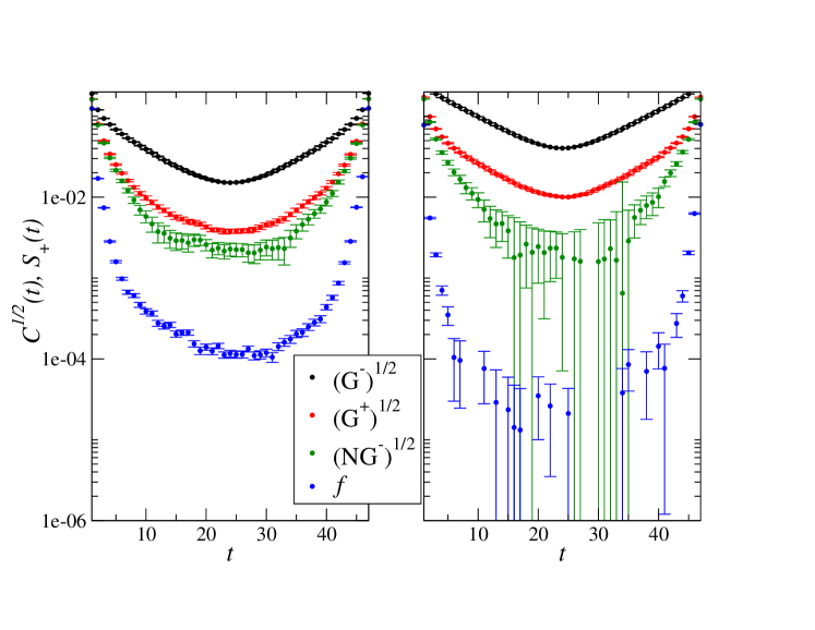
Figure 4: Timeslice correlators for $\beta=0.36$ (left) and 0.24 (right) with $ma=0.005$, $L_{s}=64$.

The data plotted corresponds to the timeslice correlators in G^- (17), G⁺ (18) and NG^- (20) meson channels, and the forwards-moving spin-${1\over 2}$ quasiparticle state given by $S_{+}=S_{0}+S_{3}$ (LABEL:eq:quasiprop), denoted $f$ in the figure. Since NG⁺ also has contributions from disconnected fermion line diagrams not calculated here, we merely comment that numerically the connected component is very close to the G^- channel (indeed they are exactly degenerate in the $m\to 0$ limit), and omit this channel from subsequent analysis. Also note we have chosen to plot the square root of the meson data in Fig. 4 for ease of comparison with $f$.

As might be anticipated from the form of (17), G^- yields numerically the largest signal, which increases going from symmetric to broken phases as first noted in [9]. A striking feature is the disparity between G^± channels, which should be degenerate if U(2) symmetry is manifest. The NG^- data is appreciably noisier, since the signal (20) results from the difference of two much larger numbers. Finally, $f$ is not symmetric under $t\mapsto-t$, a generic feature of fermion correlators. For $\beta=0.36$ the $f$ correlator has kink discontinuities about $t=6,L_{t}-6$ which are compatible with the branch cut artifacts in the free fermion correlator revealed in the difference between $C_{0}$ and $C,\tilde{C}_{0}$ in Fig. 2, discussed in Sec. 3. At the weaker coupling $\beta=0.36$ the decay in the forwards $t$-direction is comparable in all channels, modulo an overall normalisation, suggesting the mesons are weakly bound states with $M_{\rm meson}\sim 2M_{f}$. At $\beta=0.24$ it is possible to discern a difference between G and NG channels, but by now both NG and $f$ signals are much noisier. The visible curvature in all data, particularly those at weak coupling, suggests that a fit assuming conventional exponential decay resulting from an isolated simple pole may not capture all the information present. Nonetheless, as a first step in the next subsection we will pursue this strategy.

4.1 Correlator and plateau fits

We allow two Ansätze for the correlator. In the massive case we assume the usual exponential behaviour with (symmetric meson correlator) and without (non-symmetric fermion correlator) back-propagating part

$$C_{\text{sym}}(t) =a\cosh(m_{\text{eff}}(t-L_{t}/2))\,,$$ (36)

$$C_{\text{exp}}(t) =a\,\mathrm{e}^{-m_{\text{eff}}t}\,,$$ (37)

respectively, while for fermions with $m=0$ we additionally test for compatibility with an algebraic decay

$$C_{\text{alg}}(t) =\alpha t^{-\mu_{\text{eff}}}.$$ (38)

In both cases the proportionality constants $a$, $\alpha$ do not carry physical meaning, whereas the effective masses $m_{\text{eff}}$ and anomalous dimension $\mu_{\text{eff}}$ are to be determined, respectively.

To this end we use the procedure derived in Ref. [17], Appendix B and summarised in Algorithm 1 thereof. First, we calculate local approximations of the effective masses

$$m_{\text{eff}}(t) =\operatorname{cosh^{-1}}\left(\frac{C_{\text{sym}}(t+1)+C_{\text{sym}}(t-1)}{C_{\text{sym}}(t)}\right)\,,$$ (39)

$$m_{\text{eff}}(t) =-\ln\frac{C_{\text{exp}}(t+1)}{C_{\text{exp}}(t)}\,,$$ (40)

$$\mu_{\text{eff}}(t) =-\frac{\ln\frac{C_{\text{alg}}(t+1)}{C_{\text{alg}}(t)}}{\ln\frac{t+1}{t}}$$ (41)

and identify plateaus of the effective mass. Next, we fit a constant to the plateau in this region and simultaneously one of formulae (36) or (38) directly to the respective correlator in the same region. The constant plateau fit might have a bias (see [17], or for more details Sec. 4.C of [18]), so further analysis always relies on the correlator fit exclusively. Finally, if the effective mass is not too noisy, we identify all regions where its slope is compatible with zero, repeat the fit and use the standard deviation over the different regions’ fit results as an estimator of the systematic error $\Delta_{\rm syst}$.

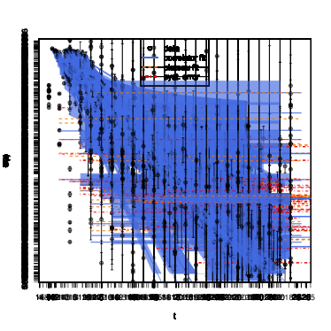
Figure 5: Visualisations of the effective mass (39) plateaus of $\cosh$-type mesonic ‘Goldstone’ $C_{1\kern-4.5pt1}(x)=C_{\rm G^{+}}(x)$ (18) correlator fits. The blue line with error band gives result of the correlator fit with statistical error, obtained via eq. (36). The length of the blue band indicates the fitting region. For comparison, a constant fit to the effective mass is shown by the dashed orange line. The dot-dashed red line shows the estimation of the systematic error, as explained in [17]. Note that the red and orange lines have been extended outside of the fitting region, for clearer visibility. Left: $m=$0.005$$, $\beta=$0.28$$, $L_{s}=80$. Right: $m=$0.005$$, $\beta=$0.36$$, $L_{s}=64$.

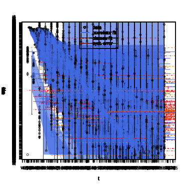
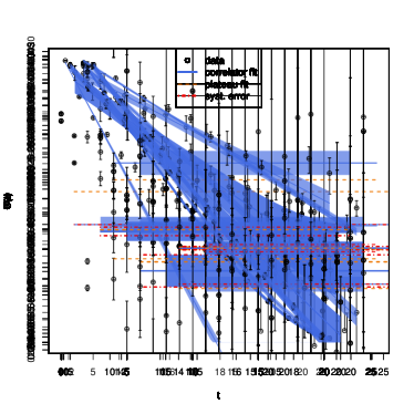
Figure 6: Algebraic fit of a fermionic correlator (38) ($m=$0$$, $\beta=$0.34$$, $L_{s}=64$). Visualisation of the effective mass (41) (left) and actual fit of the correlator (right). Fit results including statistical errors are shown in blue. The length of the blue band indicates the fitting region. For comparison, in the left panel a constant fit to the effective mass is shown by the dashed orange line.

Figure 5 shows examples of plateaus corresponding to a weakly and a strongly interacting ‘Goldstone’ meson correlator respectively. Clearly, the case of $\beta=$0.24$$ features a distinct plateau, resulting in small errors. In contrast, $\beta=$0.36$$ comes without an obvious flat region. This property is captured in a much larger systematic error, as seen in Table 1 below.

For fermions the effective mass often turns out to be too noisy to be of any use, as can be seen in the left panel of figure 6. Nevertheless a fit to the correlator is well behaved in most cases (see right panel of fig. 6), so that we can safely analyse the fit result, albeit without an estimator of potential systematic errors.

4.2 Results

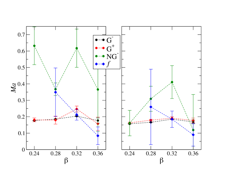
Figure 7: Spectrum results with $ma=0.005$, $L_{s}=64$ (left) and $L_{s}=80$ (right). Error bars are obtained by adding $\Delta_{\rm stat}$ and $\Delta_{\rm syst}$ in quadrature.

Fig. 7 shows the resulting spectrum in the four channels of interest for $L_{s}=64$ (left) and $L_{s}=80$ (right), using the bare fermion mass $ma=0.005$, and assuming exponential decay. Although there are relatively large uncertainties in NG^- and $f$ channels, the picture remains consistent as $L_{s}$ increases from 64 to 80. The two G channels yield roughly constant masses across the range of couplings explored; moreover despite the large disparity in signal amplitude apparent in Fig. 4, the G^± masses are approximately degenerate consistent with U(2) symmetry. The $f$ mass satisfies $M_{f}\simeq{1\over 2}M_{\rm meson}$ at the weakest coupling, but rises sharply across the critical region $\beta\sim 0.28$, consistent with dynamical mass generation associated with the spontaneous breaking of U(2). No satisfactory fits were found for the noisy broken phase data at $\beta=0.24$. The NG^- results are very noisy, but are at least consistent with $M_{\rm NG}\propto M_{f}$ as befits a generic non-Goldstone bound state.

$\beta$	$\Delta_{\rm syst}(L_{s}=64)$	$\Delta_{\rm syst}(L_{s}=80)$
0.24	0.0008	0.0007
0.28	0.0001	0.0002
0.32	0.0029	0.0003
0.36	0.0158	0.0113

Table 1: Systematic fitting uncertainties in the G^- channel with $ma=0.005$.

As mentioned above, as a consequence of the curvature of the data in the plots of Fig. 4, single-pole fits of the form (36) are more convincing in the broken phase, and work less well in the weak-coupling symmetric phase; this is corroborated by the growth $\Delta_{\rm syst}$ with $\beta$ exemplified by G^- data shown in Table 1. Mesons at weak coupling are weakly-bound at best, and ultimately may be better described using a continuum spectral function.

Qualitatively, the picture is very similar to that found in simulations of the Thirring model with $N=1$ staggered fermions (see Fig. 17 of [8]), in which case the symmetry breaking pattern is U(1)$\otimes$U(1)$\to$U(1). For DWF with finite $L_{s}$ it is necessary to enquire to what extent the anticipated pattern U(2)$\to$U(1)$\otimes$U(1) is realised.

Figure 8: $M_{{\rm G}^{-}}$ vs. $m$ for various couplings (left); comparison of $M_{{\rm G}^{\pm}}$ vs. $m$ (right). In both cases open symbols denote $L_{s}=64$, closed $L_{s}=80$.

Fig. 8 addresses this issue from two directions. On the left is plotted the Goldstone versus bare fermion masses. Although $M_{\rm G}^{-}$ decreases with $m$ at all couplings, there is no sign of the $M_{\rm G}\propto\surd m$ behaviour of a true Goldstone mode in the broken phase $\beta=0.24$. Comparison of $L_{s}=64,80$ also suggests the results are not yet in the large-$L_{s}$ limit where U(2) recovery is expected. The plot on the right compares data from the two Goldstone channels G^±, which with U(2) symmetry manifest should be degenerate even for $m\not=0$. At best degeneracy looks to be recovered only as $m\to 0$, and again there are significant finite-$L_{s}$ effects. We conclude the results obtained in the meson sector are suggestive but not yet conclusive, and that U(2) symmetry recovery is not yet demonstrated.

In summary, in this section we have demonstrated: the presence of meson bound states (unambiguously in the broken phase $\beta<\beta_{c}$, more equivocally in the symmetric phase $\beta>\beta_{c}$); degeneracy of the two distinct Goldstone states in pseudoscalar and scalar channels, despite the large numerical disparity in the correlators; the expected hierarchy between G and NG states; the evolution in fermion mass from weak coupling where mesons are weakly-bound $f\bar{f}$ states to strong coupling where there is dynamical gap generation and $M_{f}$ is hard to measure. The scaling of the Goldstone masses with bare fermion mass does not manifest the expected $M_{G}\propto\surd m$ behaviour, and further work to explore both thermodynamic and large-$L_{s}$ limits is needed.

5 Conformal Nature of the Fermion Correlator

While spectroscopy with explicit U(2) symmetry-breaking $m\not=0$ is the best way to test the Goldstone nature of the bound states G^±, it does not reveal the critical nature of the fermion at the fixed point. In this section we discuss the case $m=0$, presenting both continuum-based models for the critical propagator, characterised by a new and distinct exponent $\eta_{\psi}$, and numerical data for the propagator $S_{0}$ (LABEL:eq:quasiprop) taken in the massless limit.

5.1 Massless fermions

To begin, we propose a model for the fermion timeslice correlator $C_{f}(x_{0})$ in the symmetric phase $g^{2}<g_{c}^{2}$ in the massless limit $m\to 0$. In this regime we expect the correlator to decay algebraically, but also to reflect in some way a finite correlation length which diverges only as $g^{2}\to g^{2}_{c-}$. Our ultimate aim is to identify the fermion anomalous dimension $\eta_{\psi}$ defined by the critical scaling

$$C_{f}(\vec{p})\sim{{\hat{p}\cdot\vec{\gamma}}\over{|\vec{p}|^{1-{\eta_{\psi}}}}}\;\;\;\Leftrightarrow\;\;\;C_{f}(\vec{x})\sim{{\hat{x}\cdot\vec{\gamma}}\over{|\vec{x}|^{2+{\eta_{\psi}}}}}$$ (42)

with $\vec{\gamma}=(\gamma_{0},\gamma_{1},\gamma_{2})$, $\hat{x}\cdot\vec{x}=|\vec{x}|\equiv x$.

We start by focussing on the behaviour exactly at the critical point, modelled by replacing the free massless fermion momentum-space propagator $1/ip{\!\!\!/}$ by $1/ip^{1-\eta_{\psi}}\hat{p}_{\mu}\gamma_{\mu}$ with $|\hat{p}|=1$ and $\hat{p}_{\mu}p_{\mu}=p$:

$$C_{f}(x) = {\rm tr}\left\{{\gamma_{\hat{x}}\over 4}\int{{d^{3}p}\over{(2\pi)^{3}}}{{-i\hat{p}_{\mu}\gamma_{\mu}}\over{p^{1-\eta_{\psi}}}}e^{i\vec{p}\cdot\vec{x}}\right\}$$ (43)

$$= \int{dp\over 8\pi^{2}}p^{1+\eta_{\psi}}\int_{-{\pi\over 2}}^{\pi\over 2}d\theta\sin 2\theta\sin(px\cos\theta)$$

$$= {x^{-{1\over 2}}\over{(2\pi)^{3\over 2}}}\int_{0}^{\infty}dpp^{{1\over 2}+\eta_{\psi}}J_{3\over 2}(px).$$

The remaining integral over $p$ is formally given by

$$C_{f}(x)={1\over{4\pi x^{2+\eta_{\psi}}}}{{\Gamma(2+\eta_{\psi})}\over{\Gamma(1+{{\eta_{\psi}}\over 2})\Gamma(1-{{\eta_{\psi}}\over 2})}};\;\;\;\lim_{\eta_{\psi}\to 0}C_{f}(x)={1\over{4\pi x^{2}}}.$$ (44)

Since the decay is algebraic, it is natural to plot $C_{f}(x)$ using logarithmic scales on both $x$ and $y$-axes.

5.2 UV considerations

The integral (43) is only convergent for $\eta_{\psi}<0$: in general therefore we must introduce a UV scale $\Lambda$ to regularise the model. A simple sharp momentum-space cutoff $p\leq\Lambda$ yields an oscillatory dependence $C_{f}(x)\propto\cos(\Lambda x)$, which is physically unacceptable. We have explored a smoother cutoff defined by the following integral, which exists for $\eta_{\psi}>-3$:

$${x^{-{1\over 2}}\over{(2\pi)^{3\over 2}}}\int_{0}^{\infty}dpp^{{1\over 2}+\eta_{\psi}}J_{3\over 2}(px)e^{-{p^{2}\over\Lambda^{2}}}={{\Gamma({{3+\eta_{\psi}}\over 2})}\over{12\pi^{2}}}x\Lambda^{3+\eta_{\psi}}M\left(\textstyle{{{3+\eta_{\psi}}\over 2};{5\over 2};-{{x^{2}\Lambda^{2}}\over 4}}\right),$$ (45)

where $M$ is the confluent hypergeometric function ${}_{1}F_{1}$. In the limit $x\Lambda\to\infty$ (45) recovers the naive algebraic decay (44).

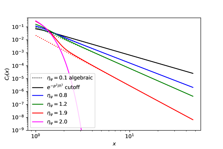
Figure 9: $C_{f}(x)$ for various $\eta_{\psi}$ with $\Lambda=\pi$.

Fig. 9 shows $C_{f}(x)$ evaluated using both (44,45). To approximate the lattice cutoff we choose a numerical value $\Lambda=\pi$. For $\eta_{\psi}\raisebox{-2.15277pt}{$\ \stackrel{{\scriptstyle\textstyle<}}{{\textstyle\sim}}\ $}1$ the regularised form matches the algebraic form well, but for larger values of $\eta_{\psi}$ the cutoff dependence is significant over much of the range permitted by $L_{t}=48$. As dictated by the gamma function in the denominator of (44), things break down at $\eta_{\psi}=2$ where (45) has the limiting form

$$C_{f}(x)={{x\Lambda^{5}}\over{16\pi\surd\pi}}\exp\left(-{{x^{2}\Lambda^{2}}\over 4}\right),$$ (46)

and it is no longer possible to hide the cutoff.

We conclude: (i) for conformal dynamics described by (42) there appears to be an upper bound on the anomalous dimension $\eta_{\psi}<2$; (ii) for large anomalous dimensions UV artifacts might make fitting for $\eta_{\psi}$ a non-trivial challenge.

5.3 Introduction of finite correlation length

Next we introduce a finite correlation length $\mu^{-1}$, motivated by the large-$N$ limit of the scalar auxiliary field propagator found in the 2+1$d$ Gross-Neveu model [19]:

$$D_{\sigma}(p)={4\mu\over{p+\mu}},$$ (47)

where the inverse correlation length $\mu$ is related to the width of an unstable resonance in the scalar channel, but does not correspond to a pole on the imaginary-$p$ axis yielding exponential decay. Rather, the appearance of $p=(\vec{p}\cdot\vec{p})^{1\over 2}$ in the denominator yields a branch cut starting at the origin in the complex $p^{2}$ plane; the pole of (47) at $(p^{2})^{1\over 2}=-\mu$ lies on a different sheet to the one where the integral defining the Fourier transform from $p$ to $x$ lives. This form was used to fit numerical $D_{\sigma}$ data in [20].

Our Ansatz for the fermion propagator in momentum space is

$$C_{f}(p)={1\over{i(p+\mu)^{1-\eta_{\psi}}\hat{p}_{\mu}\gamma_{\mu}}}={{-i\hat{p}_{\mu}\gamma_{\mu}}\over{(p+\mu)^{1-\eta_{\psi}}}}.$$ (48)

In real space we now have

$$C_{f}(x)={1\over 4}{\rm tr}\gamma_{\hat{x}}C_{f}(p)={x^{-{1\over 2}}\over{(2\pi)^{3\over 2}}}\int_{0}^{\infty}dp(p+\mu)^{\eta_{\psi}-1}p^{3\over 2}J_{3\over 2}(px).$$ (49)

In the limit $\mu\to 0$ we recover (44), while for $\mu\to\infty$

$$C_{f}(x)={1\over{\pi^{2}\mu^{1-\eta_{\psi}}x^{3}}}.$$ (50)

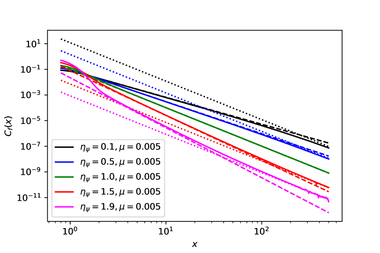
Figure 10: $C_{f}(x)$ for various $\eta_{\psi}$ with $\Lambda=\pi$ and $\mu=0.005$.

Once again a UV regulator $e^{-{p^{2}\over\Lambda^{2}}}$ must be introduced, which modifies $C_{f}(x)$ at small $x$. The resulting integral may be evaluated using numerical quadrature; the result for fixed $\mu$ and varying $\eta_{\psi}\in(0,2)$ is shown in Fig. 10. Dashed and dotted lines show the limiting forms (44) and (50) respectively.

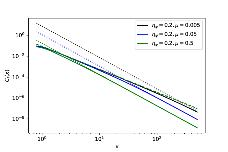
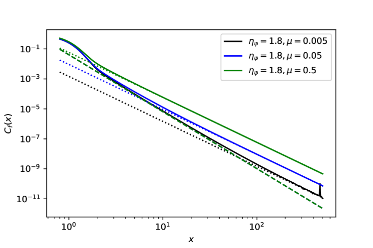
Figure 11: $C_{f}(x)$ for $\eta_{\psi}=0.2$ with $\Lambda=\pi$ and various $\mu$.

Figure 12: $C_{f}(x)$ for $\eta_{\psi}=1.8$ with $\Lambda=\pi$ and various $\mu$.

In practice, our dataset is hypothesised to have fixed $\eta_{\psi}$ and varying $\mu$ corresponding to varying $g_{c}^{-2}-g^{-2}$. Figs. 12, 12, show $C_{f}(x)$ evaluated for various $\mu$ with fixed $\eta_{\psi}$ chosen close to the extremes of the range (0,2). The curvature of the plots suggests it may be possible to distinguish the cases $\eta_{\psi}<1$ and $\eta_{\psi}>1$ by qualitative means without recourse to a fitting analysis where control of systematics is still poorly understood.

However, the Monte Carlo data is for the timeslice correlator $C_{ft}(x_{0})$. For $C_{f}(x)=\hat{x}\cdot\vec{\gamma}/x^{2+\eta_{\psi}}$,

$$C_{ft}(x_{0})={1\over 4}{\rm tr}\gamma_{0}\int d^{2}x_{\perp}C_{f}(x)={{2\pi}\over{1+\eta_{\psi}}}{1\over x_{0}^{\eta_{\psi}}}.$$ (51)

We therefore predict the slope of the resulting data on a log-log plot to be in the range (0,2) for $\Lambda x_{0}\gg 1$, $\mu x_{0}\ll 1$, with asymptotic slope 1 achieved for $\mu x_{0}\gg 1$.

5.4 Numerical results

We calculated the fermion timeslice propagator with $m=0$ using just the time-symmetric projection $S_{0}$ of (LABEL:eq:quasiprop) on ensembles with $L_{s}=64$ generated by 5000 RHMC trajectories taken at 5 $\beta$-values in the symmetric phase, with the strongest $\beta=0.28$ corresponding approximately to the critical value obtained in studies of the equation of state [6, 7].

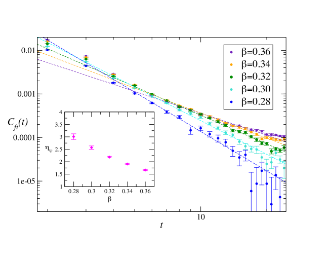
Figure 13: Timeslice fermion correlator for various $\beta$ with $L_{s}=64$, $m=0$, together with fits to (38). The inset shows the fitted anomalous dimension $\eta_{\psi}$.

The results for data averaged over forwards and backwards directions are shown on a log-log plot in Fig. 13. Whilst the data show qualitative features which might be compared with those of Fig. 12 describing the case $\eta_{\psi}>1$, the signal-to-noise ratio falls as the critical coupling is approached.

In principle on a lattice of finite temporal extent we should correct for backwards propagating signals, and also contributions from propagation over arbitrarily many temporal circuits. The analysis presented in Appendix C shows that both effects are mitigated by fermion antiperiodic boundary conditions; however, with the limited statistical precision currently achieved there is no motivation to explore beyond the simplest fit form (38). Results for the fitted $\eta_{\psi}=\mu_{\rm eff}$ are plotted in the inset of Fig. 13. The quality of fit increases as $\beta\searrow\beta_{c}$ and the fitted $\eta_{\psi}\simeq 3$ for the near-conformal value $\beta=0.28$.

In summary, we have established a signal and obtained results for the fermion timeslice correlator in the vicinity of the postulated QCP in the massless limit, and analysed its propagation assuming algebraic decay in the temporal direction. Our results are in qualitative agreement with the model presented in Sec. 5.3, but disagree quantitively in two respects: firstly the value for the fermion anomalous dimension $\eta_{\psi}$ lies outside the range [0,2) compatible with the conformal propagator in momentum space (42); secondly there is no sign of recovery of $\mu_{\rm eff}=1$ far from criticality as predicted by (48,50). Rather, our data suggest $\eta_{\psi}\approx 3$ in the vicinity of the QCP, an unexpectedly large value.

6 Discussion

In this paper we have used the DWF formulation of the Thirring model to perform spectroscopy using orthodox lattice field theory techniques on a lattice in which the temporal extension is greater than the spatial extent. Since the Thirring model has no gauge symmetry, we have also been able to study propagation of elementary fermion fields. In both cases the results represent significant progress over previous exploratory studies [5, 9].

In the meson sector, our results are consistent with the two Goldstone-like modes G^± having degenerate masses, as demanded by the residual U(1)$\otimes$U(1) symmetry, despite a large disparity in the overall magnitude of the correlators. Moreover the accessible non-Goldstone NG^- state is clearly more massive, and increasing as the system moves from the symmetric into the broken phase, despite a very noisy signal due to its definition in terms of the difference of two much larger correlators. At the weakest couplings $\beta=0.36$ explored, the poor quality of fit reflected in the large systematic error $\Delta_{\rm syst}$ suggests mesons are only very weakly bound so there is significant contamination from a fermion-antifermion continuum. In the broken phase at $\beta=0.24$ by contrast, the Goldstones are tightly bound, but fail to respect the expected behaviour $M_{\rm G}\propto\surd m$; the large $L_{s}$-artifacts shown in Fig. 8 suggest U(2) symmetry restoration may be even harder to observe in the spectrum than in the order parameter: studies in the thermodynamic limit, not taken here, may also prove important.

In the fermion sector, we have first presented an analysis of the free-field correlator which highlights a potentially significant contamination arising from a fermion-doubler continuum at small $t$, clearly visible in the data of Fig. 4, which must be taken into account when performing spectroscopic fits. We also examined the impact of varying domain wall height $M$ and separation $L_{s}$. Once again, the superior convergence of the DWF formulation with mass term $S_{m_{3}}$ (7) is apparent. A major innovation has been the employment of wall sources to vastly improve the sampling of the correlator over previous attempts [5]. The results indicate $M_{f}\approx{1\over 2}M_{\rm G}\simeq{1\over 2}M_{\rm NG}$ at weak coupling $\beta=0.36$, consistent with mesons being weakly bound states, but that $M_{f}$ rises steeply towards the phase transition at $\beta_{c}\approx 0.28$ until correlator noise precludes its measurement in the broken phase. It is clear a much finer comb of coupling strengths in the vicinity of $\beta_{c}$ is needed in order to refine this rather crude first step.

Finally we exploited the stability of the DWF formulation to perform measurements of the fermion propagator in the $m\to 0$ limit in an attempt to probe the conformal nature of the putative fixed point dynamics. We first presented an analytic model demonstrating that in general a UV regularisation is needed, and that the algebraic decay of the fermion correlator parametrised by the critical exponent $\eta_{\psi}$ needs to satisfy the bounds $0\leq\eta_{\psi}<2$ in order to permit a straightforward passage between real space and momentum space. The numerical data of Fig. 13 by contrast prefer $\eta_{\psi}\approx 3$. We are at a loss to account for this discrepancy, but know of no reason why a conformal field theory with such a large anomalous dimension should be excluded. This is certainly the most interesting result of this paper, and contrasts markedly with the value $\eta_{\psi}=0.37(1)$ found in finite volume scaling studies of both Thirring [21] and U(1) Gross-Neveu [22] models formulated with staggered fermions, strengthening our conviction that DWF and staggered Thirring models are distinct.

In conclusion, while much insight into the excitations of the Thirring model as the U(2) limit is approached as $L_{s}\to\infty$ has been obtained, some important questions remain unanswered. In future work, encouraged by the apparent superior $L_{s}$ convergence observed in [23], we plan to extend the study to the Thirring model formulated with DWF using a Wilson kernel rather than the simplest Shamir kernel (5) used here.

Data Access

All the code and data (raw as well as analysed) required to reproduce the results of this paper can be found in [24] under open access. We used Fortran for the DW simulations and heavily relied on the hadron [25] package for our data analysis implemented in R [26].

Appendix A Derivation of the free fermion propagator in time

A.1 List of auxiliary variables

The auxiliary variables required in the equations (24) and (25) are given by

$$2\cosh\alpha =\frac{1+b^{2}+\bar{p}^{2}}{b}\,; \bar{p}_{\mu} =\sin p_{\mu}\,; b(p) =1-M+\sum_{\mu}(1-\cos p_{\mu})$$ (52)

as well as

$$A_{\pm} =\Delta^{-1}B\left(\mathrm{e}^{\pm\alpha}-b\right)\left(1-|m|^{2}\right)\,,$$ (53)

$$A_{m} =\Delta^{-1}B\left[-2mb\sinh\alpha+\mathrm{e}^{-\alpha(L_{s}-1)}\left(\mathrm{e}^{-2\alpha}(b-\mathrm{e}^{\alpha})+|m|^{2}(\mathrm{e}^{-\alpha}-b)\right)\right]\,,$$ (54)

$$B =(2b\sinh\alpha)^{-1}\,,$$ (55)

$$\begin{split}\Delta&=\mathrm{e}^{2\alpha}(b-\mathrm{e}^{-\alpha})+|m|^{2}(\mathrm{e}^{\alpha}-b)\\ &\quad+\mathrm{e}^{-2\alpha(L_{s}-1)}\left[|m|^{2}(b-\mathrm{e}^{-\alpha})+\mathrm{e}^{-2\alpha}(\mathrm{e}^{\alpha}-b)\right]\\ &\quad+\delta_{m,m_{h}}\,\mathrm{e}^{-\alpha(L_{s}-1)}4mb\sinh\alpha\,.\end{split}$$ (56)

The mass can be chosen to be either $m=m_{h}$ or $m=im_{3}$.

A.2 Holomorphic case up to poles

We employ the Matsubara technique

$$C_{0}(t) =\frac{1}{L_{t}}\sum_{p_{0}}\frac{1+n(m)\cos p_{0}}{m+i\sin p_{0}}\mathrm{e}^{ip_{0}t}$$ (57)

$$=\frac{-1}{2\pi i}\oint_{\mathcal{C}}\mathrm{d}z\,\frac{1}{\mathrm{e}^{L_{t}z}+1}\frac{1+n(m)\cos(-iz)}{m+i\sin(-iz)}\mathrm{e}^{zt}$$ (58)

$$=\frac{-1}{2\pi i}\oint_{\mathcal{C}}\mathrm{d}z\,\frac{\mathrm{e}^{zt}}{\mathrm{e}^{L_{t}z}+1}\frac{1+n(m)\cosh z}{m+\sinh z}$$ (59)

where the closed contour $\mathcal{C}$ has to be chosen such that it encloses the poles of the Fermi-Dirac function $\frac{1}{\mathrm{e}^{L_{t}z}+1}$ corresponding to the Matsubara frequencies $z=ip_{0}=i\frac{2\pi}{L_{t}}\left(j+\frac{1}{2}\right)$ with $j=0,\dots,L_{t}-1$ and no other poles, as visualised in figure 14.

Figure 14: Initial contour $\mathcal{C}$ from eq. (59) enclosing the poles of the Fermi-Dirac function $\frac{1}{\mathrm{e}^{L_{t}z}+1}$.

The integrand is $2\pi i$-periodic (reflecting the finite momenta range due to the lattice discretisation) and has singularities at $z=i\frac{2\pi}{L_{t}}\left(\mathbb{Z}+\frac{1}{2}\right)$, $z=-\operatorname{sinh^{-1}}m+i2\pi\mathbb{Z}$, and at $z=\operatorname{sinh^{-1}}m+i\pi+i2\pi\mathbb{Z}$. The two former are poles of first order whereas the latter can be lifted, i.e.the numerator is zero as well, which corresponds to the disappearance of the doubler or back-propagating part (opposite real mass) and is exactly the reason we had to introduce the normalisation $n(m)$. Thus we can safely deform the contour $\mathcal{C}$ to the four paths shown in figure 15

$$\mathcal{C}_{1} =\mathbb{R}+i\varepsilon\,,$$ (60)

$$\mathcal{C}_{2} =\left[\infty+i\varepsilon,\,\infty+2\pi i-i\varepsilon\right]\,,$$ (61)

$$\mathcal{C}_{3} =-\mathbb{R}+2\pi i-i\varepsilon\,,$$ (62)

$$\mathcal{C}_{4} =\left[-\infty+2\pi i-i\varepsilon,\,-\infty+i\varepsilon\right]\,.$$ (63)

This means that we first integrate along the real axis shifted upwards by the infinitesimal imaginary parameter $i\varepsilon$. Then at positive real infinity we go upwards to imaginary $2\pi i-i\varepsilon$. Next we go in negative direction parallel to the real axis. Finally we close the contour at negative real infinity going back down to the imaginary part $i\varepsilon$.

Figure 15: Deformed contour $\mathcal{C}_{1}\cup\mathcal{C}_{2}\cup\mathcal{C}_{3}\cup\mathcal{C}_{4}$.

Let us consider $\mathcal{C}_{2}$ and $\mathcal{C}_{4}$ first. $t=0,\dots,L_{t}-1$, therefore at positive real infinity the integrand is exponentially suppressed by the Fermi-Dirac function, so $\mathcal{C}_{2}$ does not give any contribution. The integral along $\mathcal{C}_{4}$, in contrast, does not vanish for $t=0$. At negative real infinity the $\sinh$- and $\cosh$-terms dominate and the Fermi-Dirac function goes to one. So we get

$$\frac{-1}{2\pi i}\int_{\mathcal{C}_{4}}\mathrm{d}z\,\frac{\mathrm{e}^{zt}}{\mathrm{e}^{L_{t}z}+1}\frac{1+n(m)\cosh z}{m+\sinh z}=\frac{-1}{2\pi i}\int\limits_{-\infty+2\pi i-i\varepsilon}^{-\infty+i\varepsilon}\mathrm{d}x\,\frac{\mathrm{e}^{tx}}{\mathrm{e}^{L_{t}x}+1}\frac{1+n(m)\cosh x}{m+\sinh x}\\ =\frac{-1}{2\pi i}\int\limits_{2\pi i-i\varepsilon}^{i\varepsilon}\mathrm{d}x\left(-\delta_{t0}\right)=\frac{\delta_{t0}}{2\pi i}\left(i\varepsilon-\left(2\pi i-i\varepsilon\right)\right)=-\delta_{t0}$$ (64)

for $\varepsilon\rightarrow 0$.

$\mathrm{e}^{N_{t}z}$ and $\sinh^{2}\frac{z}{2}$ are both $2\pi i$-periodic. Thus integrating along $\mathcal{C}_{3}$ is identical to integrating along the real axis shifted by $-i\varepsilon$. The union $\mathcal{C}_{1}\cup\mathcal{C}_{3}-2\pi i$ together with infinitesimal closing sequences at $\pm\infty$ is again a closed contour $\mathcal{C^{\prime}}$ around the real axis winding once in negative direction (see fig.16). The corresponding integral can be performed using the residuum theorem and plugging in the single real first order pole $z_{0}=-\operatorname{sinh^{-1}}m$. We get

$$\frac{-1}{2\pi i}\oint_{\mathcal{C^{\prime}}}\mathrm{d}z\,\frac{\mathrm{e}^{zt}}{\mathrm{e}^{L_{t}z}+1}\frac{1+n(m)\cosh z}{m+\sinh z} =\operatorname{Res}_{z_{0}}\frac{\mathrm{e}^{zt}}{\mathrm{e}^{L_{t}z}+1}\frac{1+n(m)\cosh z}{m+\sinh z}$$ (65)

$$=\lim_{z\rightarrow z_{0}}\frac{\mathrm{e}^{zt}}{\mathrm{e}^{L_{t}z}+1}\left(1+n(m)\cosh z\right)\frac{z-z_{0}}{m+\sinh z}$$ (66)

$$=\frac{\mathrm{e}^{-\operatorname{sinh^{-1}}mt}}{\mathrm{e}^{-\operatorname{sinh^{-1}}mL_{t}}+1}\frac{1+n(m)\cosh\operatorname{sinh^{-1}}m}{\cosh\operatorname{sinh^{-1}}m}$$ (67)

$$=\frac{\mathrm{e}^{-\tilde{m}t}}{\mathrm{e}^{-\tilde{m}L_{t}}+1}\frac{2}{\sqrt{1+m^{2}}}\,,$$ (68)

where $\tilde{m}\coloneqq\operatorname{sinh^{-1}}m$.

Figure 16: Alternative closed contour $\mathcal{C^{\prime}}\supset\mathcal{C}_{1}\cup\mathcal{C}_{3}-2\pi i$.

Now we have all the ingredients to evaluate equation (59). It yields

$$C_{0}(t) =\frac{-1}{2\pi i}\oint_{\mathcal{C}}\mathrm{d}z\,\frac{\mathrm{e}^{zt}}{\mathrm{e}^{L_{t}z}+1}\frac{1+n(m)\cosh z}{m+\sinh z}$$ (69)

$$=\frac{-1}{2\pi i}\left(\int_{\mathcal{C}_{4}}\mathrm{d}z+\oint_{\mathcal{C^{\prime}}}\mathrm{d}z\right)\frac{\mathrm{e}^{zt}}{\mathrm{e}^{L_{t}z}+1}\frac{1+n(m)\cosh z}{m+\sinh z}$$ (70)

$$=\frac{\mathrm{e}^{-\tilde{m}t}}{\mathrm{e}^{-\tilde{m}L_{t}}+1}\frac{2}{\sqrt{1+m^{2}}}-\delta_{t0}\,.$$ (71)

A.3 Case including branch cuts

By and large, the derivation of $C_{h}(t)$ proceeds in the same way as that of $C_{0}(t)$ until the integral over $\mathcal{C}^{\prime}$ has to be solved. This part turns out to be trickier as the paths $\mathcal{C}_{1}$ and $\mathcal{C}_{3}-2\pi i$ cannot be connected at $\pm\infty$ because of the aforementioned branch cuts on the real axis starting at $\pm\operatorname{cosh^{-1}}\frac{5}{4}=\pm\ln 2$. Instead we have to split both paths into three parts each

$$\mathcal{C}_{1,3}^{-} =\left[-\infty\pm i\varepsilon,\,-\ln 2\pm i\varepsilon\right]\,,$$ (72)

$$\mathcal{C}_{1,3}^{0} =\left[-\ln 2\pm i\varepsilon,\,\ln 2\pm i\varepsilon\right]\,,$$ (73)

$$\mathcal{C}_{1,3}^{+} =\left[\ln 2\pm i\varepsilon,\,\infty\pm i\varepsilon\right]$$ (74)

and bridge the gaps between them with infinitesimal paths orthogonal to the real axis as in figure 17. Thus we are left with $\mathcal{C}_{1}^{0}\cup\mathcal{C}_{3}^{0}$ enclosing the pole at $z=-\operatorname{sinh^{-1}}m$ and yielding the same contribution as the integral over $\mathcal{C}^{\prime}$, as well as the two paths along the branch cuts

$$\mathcal{C}_{\text{bc}}^{\pm} \coloneqq\mathcal{C}_{1}^{\pm}\cup\mathcal{C}_{3}^{\pm}\,.$$ (75)

Figure 17: Split contours eqs. 72, 73 and 74 accounting for the branch cuts.

Taking into account the integration directions dictated by the paths, we obtain

$$\frac{-1}{2\pi i}\int_{\mathcal{C}_{\text{bc}}^{\pm}}\mathrm{d}z\,\frac{\mathrm{e}^{zt}}{\mathrm{e}^{L_{t}z}+1}C_{h}(-iz) =\frac{1}{\pi}\,\Im\int_{\pm\ln 2}^{\pm\infty}\mathrm{d}x\,\frac{\mathrm{e}^{tx}}{\mathrm{e}^{L_{t}x}+1}C_{h}(-ix)$$ (76)

$$=\pm\frac{1}{\pi}\,\Im\int_{\ln 2}^{\infty}\mathrm{d}x\,\frac{\mathrm{e}^{\pm tx}}{\mathrm{e}^{\pm L_{t}x}+1}C_{h}(\mp ix)$$ (77)

$$\approx\pm\frac{1}{\pi}\,\Im\int_{\ln 2}^{\infty}\mathrm{d}x\,\frac{\mathrm{e}^{\pm tx}}{\mathrm{e}^{\pm L_{t}x}+1}\frac{\sqrt{5-4\cosh x}}{m\pm\sinh x}$$ (78)

$$=\pm\frac{1}{\pi}\int_{\ln 2}^{\infty}\mathrm{d}x\,\frac{\mathrm{e}^{\pm tx}}{\mathrm{e}^{\pm L_{t}x}+1}\frac{\sqrt{4\cosh x-5}}{m\pm\sinh x}\,.$$ (79)

To the best of our knowledge this integral has no exact analytic solution, so we used an approximation again, this time taking the scaling near $\ln 2$ and the asymptotic behaviour into account:

$$\frac{-1}{2\pi i}\int_{\mathcal{C}_{\text{bc}}^{+}}\mathrm{d}z\,\frac{\mathrm{e}^{zt}}{\mathrm{e}^{L_{t}z}+1}C_{h}(-iz) \approx\frac{1}{\pi}\int_{0}^{\infty}\mathrm{d}x\,\frac{2^{t-L_{t}}}{m+\frac{3}{4}}\sqrt{3x}\,\mathrm{e}^{-\left(L_{t}-t+\frac{3}{4}\right)x}$$ (80)

$$=\sqrt{\frac{3}{4\pi}}\frac{1}{m+\frac{3}{4}}\frac{2^{t-L_{t}}}{\left(L_{t}-t+\frac{3}{4}\right)^{3/2}}\,,$$ (81)

$$\frac{-1}{2\pi i}\int_{\mathcal{C}_{\text{bc}}^{-}}\mathrm{d}z\,\frac{\mathrm{e}^{zt}}{\mathrm{e}^{L_{t}z}+1}C_{h}(-iz) \approx-\frac{1}{\pi}\int_{0}^{\infty}\mathrm{d}x\,\frac{2^{-t}}{m-\frac{3}{4}}\sqrt{3x}\,\mathrm{e}^{-\left(t+\frac{3}{4}\right)x}$$ (82)

$$=\sqrt{\frac{3}{4\pi}}\frac{1}{\frac{3}{4}-m}\frac{2^{-t}}{\left(t+\frac{3}{4}\right)^{3/2}}\,.$$ (83)

Appendix B Algorithmic parameters $M$ and $L_{s}$

B.1 Influence of the Domain wall height $M$

The domain wall height $M$ has a significant impact on the propagators. For reasons of space we withhold the complete formula analogous to equation (29) and limit the discussion to numerical observations.

In Fig. 18 we show the time dependent propagator for different domain wall heights where $C=C_{h}\equiv C_{3}$ is again calculated exactly.

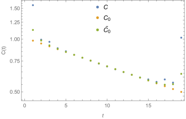
Figure 18: Exact and approximate free fermion propagators at zero spatial momentum in real space, bare mass $m=$0.05$$, $C_{0}$ and $\tilde{C}_{0}$ rescaled as in eq. (84), $m$ rescaled as in eq. (85). Domain wall heights top: $M=$0.25$$, $M=$0.5$$; bottom: $M=$0.75$$, $M=$1.5$$.

In order to approximate $C$, we have rescaled the approximate correlators

$$C_{0}(t) \mapsto\left(1-(1-M)^{2}\right)C_{0}(t)$$ (84)

and likewise for $\tilde{C}_{0}$, as well as the bare mass

$$m \mapsto m\left(1-(1-M)^{2}\right)\,.$$ (85)

We do not provide an analytic proof for the above formulæ, though hard staring at the propagator-like terms (22) in Ref. [5] supports their plausibility. With this additional modification $C$ is well approximated by $C_{0}$ even for small domain wall heights $M\sim$0.25$$ as seen in Fig. 18. The relative significance of the branch cut modelled by $\tilde{C}_{0}$, by contrast, is sensitive to $M$. $C$ shows rather unintuitive behaviour around the limits $t\approx 0$ and $t\approx L_{t}$. The deviations from the scaling at intermediate times, though always positive, appear to be smallest around $M\approx$0.5$$.

B.2 Influence of the Domain wall separation $L_{s}$

The finite-$L_{s}$ correction of $O(\mathrm{e}^{-\alpha L_{s}})$ in $C_{h}$, with $\alpha(p)$ defined in (52), reads

$$\begin{split}-&\left[4\sin^{2}{\textstyle\frac{p_{0}}{2}}\left(-3P+2\cos p_{0}\left(P+2\right)-5\right)\right.\\ &\quad\times\left(3m^{2}\left(P+1\right)-\cos 2p_{0}\left(m^{2}\left(P+5\right)+3P+13\right)+\cos p_{0}\left(3m^{2}+16P+47\right)\right.\\ &\left.\left.+m\left(m\cos 3p_{0}-4i\sin p_{0}\left(\cos 2p_{0}-2\left(P+4\right)\cos p_{0}+3P+8\right)\right)+\cos 3p_{0}-13P-35\right)\right]\\ &\left[\left(-2\cos p_{0}+P+3\right)(\cos p_{0}-1)\right.\\ &\quad\left.\times\left(m^{2}P-2\cos p_{0}\left(-m^{2}+P+3\right)-\left(m^{2}-1\right)\cos 2p_{0}+2P+5\right)^{2}\right]^{-1}\end{split}$$ (86)

with $P(p_{0})\equiv\sqrt{5-4\cos p_{0}}$, and the corresponding term in $C_{3}$ reads

$$\begin{split}&\left[4\sin^{2}{\textstyle\frac{p_{0}}{2}}\left(-3P+2\cos p_{0}\left(P+2\right)-5\right)\right.\\ &\left.\times\left(-2i\cos p_{0}\left(2m^{2}+P+2\right)+i\left(2m^{2}\left(P+3\right)+3P+5\right)+2m\sin p_{0}\left(-2\cos p_{0}+P+3\right)\right)\right]\\ &\left[P\left(-2\cos p_{0}+P+3\right)(\cos p_{0}-1)\right.\\ &\quad\left.\times\left(-m^{2}P+\left(m^{2}-1\right)\cos 2p_{0}+2\cos p_{0}\left(-m^{2}+P+3\right)-2P-5\right)\right]^{-1}\,.\end{split}$$ (87)

Appendix C IR considerations

The timeslice propagator measured in lattice simulations defined by $C_{ft}(x_{0})=\int d^{2}x_{\perp}C_{f}(x_{\perp},x_{0})$ can be written

$$C_{ft}(x_{0})={{\Gamma(2+\eta_{\psi})}\over{2\eta_{\psi}x_{0}^{\eta_{\psi}}\Gamma(1-{{\eta_{\psi}}\over 2})\Gamma(1+{{\eta_{\psi}}\over 2})}}=B(\eta_{\psi})x_{0}^{-\eta_{\psi}}.$$ (88)

When evaluating the timeslice correlator on a lattice of finite temporal extent $L_{t}$, because of the algebraic decay of $C_{f}(x_{0})$ it is necessary not only to include the effects of a backwards propagating signal, but also signals which have propagated $n$ times around the lattice, ie. we need to incorporate “image sources”. Each time a fermion crosses the timelike boundary it picks up a minus sign due to boundary conditions. The total is therefore

$$C_{ft}(x_{0};L) = {{B(\eta_{\psi})}\over L_{t}^{\eta_{\psi}}}\sum_{n=0}^{\infty}\left[{{(-1)^{n}}\over{\left({x_{0}\over L}+n\right)^{\eta_{\psi}}}}+{{(-1)^{n}}\over{\left(1-{x_{0}\over L}+n\right)^{\eta_{\psi}}}}\right]$$ (89)

$$= {{B(\eta_{\psi})}\over{(2L_{t})^{\eta_{\psi}}}}\sum_{s={x_{0}\over L},1-{x_{0}\over L}}\left[{\textstyle{\zeta(\eta_{\psi},{s\over 2})-\zeta(\eta_{\psi},{1\over 2}(1+s}))}\right],$$

where $\zeta(\alpha,z)$ is the Hurwitz zeta function; the difference in Eqn. (89) is convergent for $\eta_{\psi}>0$ and given by an integral suitable for numerical evaluation:

$$2^{-\eta_{\psi}}[{\textstyle{\zeta(\eta_{\psi},{s\over 2})-\zeta(\eta_{\psi},{1\over 2}(1+s))}}]={1\over{\Gamma(\eta_{\psi})}}\int_{0}^{\infty}{{z^{\eta_{\psi}-1}e^{-sz}}\over{1+e^{-z}}}dz.$$ (90)

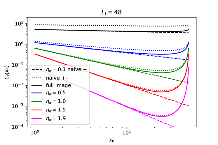
Figure 19: $C_{ft}(x_{0},L_{t})$ for various $\eta_{\psi}$ with $L_{t}=48$.

The resulting forms for $C_{ft}(x_{0};L_{t})$ are shown for various $\eta_{\psi}$ in Fig. 19. Dashed lines show the simple algebraic form (88), and dotted lines the result of a naive inclusion of just a single backwards propagating signal, as done in conventional spectroscopy. The antiperiodic boundary conditions significantly mitigate this finite-$L_{t}$ artifact, particularly for small $\eta_{\psi}$, and indeed in making the signal convergent in this limit. It is clear though that with $L_{t}=48$ it will be necessary to use a formula such as (89) for precision fitting to $\eta_{\psi}$.

References

- [1] Simon Hands “Planar Thirring Model in the U(2)-symmetric limit” In Peter Suranyi 87th Birthday Festschrift: A Life In Quantum Field Theory Singapore: World Scientific Publishing Company, 2022 arXiv:2105.09643
- [2] Andreas W. Wipf and Julian J. Lenz “Symmetries of Thirring Models on 3D Lattices” In Symmetry 14.2, 2022, pp. 333 DOI: 10.3390/sym14020333
- [3] Simon Hands “Domain wall fermions for planar physics” In Journal of High Energy Physics 2015.9 Springer ScienceBusiness Media LLC, 2015 DOI: 10.1007/jhep09(2015)047
- [4] Simon Hands “From domain wall to overlap in 2 1” In Phys. Lett. B 754, 2016, pp. 264–269 DOI: 10.1016/j.physletb.2016.01.037
- [5] Simon Hands “Towards critical physics in 2+1d with U(2N)-invariant fermions” In Journal of High Energy Physics 2016.11 Springer ScienceBusiness Media LLC, 2016 DOI: 10.1007/jhep11(2016)015
- [6] Simon Hands, Michele Mesiti and Jude Worthy “Critical behavior in the single flavor Thirring model in ” In Phys. Rev. D 102 American Physical Society, 2020 DOI: 10.1103/PhysRevD.102.094502
- [7] Simon Hands, Michele Mesiti and Jude Worthy “Critical behaviour in the single-flavor Planar Thirring Model” In PoS LATTICE2021, 2022, pp. 539 DOI: 10.22323/1.396.0539
- [8] L. Del Debbio, S. J. Hands and J. C. Mehegan “The Three-dimensional Thirring model for small N(f)” In Nucl. Phys. B 502, 1997, pp. 269–308 DOI: 10.1016/S0550-3213(97)00435-5
- [9] Simon Hands “Critical flavor number in the Thirring model” In Phys. Rev. D 99 American Physical Society, 2019 DOI: 10.1103/PhysRevD.99.034504
- [10] Stavros Christofi, Simon Hands and Costas Strouthos “Critical flavor number in the three dimensional Thirring model” In Phys. Rev. D 75, 2007, pp. 101701 DOI: 10.1103/PhysRevD.75.101701
- [11] Simon Hands “The Planar Thirring Model with Kähler-Dirac Fermions” In Symmetry 13.8, 2021, pp. 1523 DOI: 10.3390/sym13081523
- [12] Vadim Furman and Yigal Shamir “Axial symmetries in lattice QCD with Kaplan fermions” In Nuclear Physics B 439.1-2 Elsevier, 1995 DOI: 10.1016/0550-3213(95)00031-M
- [13] Ed Bennett, Simon Hands, Makis Kappas and Michele Mesiti “sa2c/thirring-rhmc: 4D parallelisation” Zenodo, 2020 DOI: 10.5281/zenodo.4016827
- [14] Paul H. Ginsparg and Kenneth G. Wilson “A remnant of chiral symmetry on the lattice” In Phys. Rev. D 25 American Physical Society, 1982 DOI: 10.1103/PhysRevD.25.2649
- [15] R. V. Gavai and Sayantan Sharma “Thermodynamics of free domain wall fermions” In Physical Review D 79.7 American Physical Society (APS), 2009 DOI: 10.1103/physrevd.79.074502
- [16] Michael E. Peskin and Daniel V. Schroeder “An Introduction to quantum field theory” Reading, USA: Addison-Wesley, 1995
- [17] Johann Ostmeyer et al. “Semimetal–Mott insulator quantum phase transition of the Hubbard model on the honeycomb lattice” In Phys. Rev. B 102 American Physical Society, 2020, pp. 245105 DOI: 10.1103/PhysRevB.102.245105
- [18] Johann Ostmeyer “The Hubbard Model on the Honeycomb Lattice with Hybrid Monte Carlo” arXiv, 2021 DOI: 10.48550/ARXIV.2110.15432
- [19] Yoshio Kikukawa and Koichi Yamawaki “Ultraviolet Fixed Point Structure of Renormalizable Four Fermion Theory in Less Than Four-dimensions” In Phys. Lett. B 234, 1990, pp. 497 DOI: 10.1016/0370-2693(90)92046-L
- [20] Simon Hands, Aleksandar Kocic and John B. Kogut “Four Fermi theories in fewer than four-dimensions” In Annals Phys. 224, 1993, pp. 29–89 DOI: 10.1006/aphy.1993.1039
- [21] Shailesh Chandrasekharan and Anyi Li “Fermion bags, duality and the three dimensional massless lattice Thirring model” In Phys. Rev. Lett. 108, 2012, pp. 140404 DOI: 10.1103/PhysRevLett.108.140404
- [22] Shailesh Chandrasekharan and Anyi Li “Quantum critical behavior in three dimensional lattice Gross-Neveu models” In Phys. Rev. D 88, 2013, pp. 021701 DOI: 10.1103/PhysRevD.88.021701
- [23] Jude Worthy and Simon Hands “Properties of Overlap and Domain Wall Fermions in the 2+1D Thirring Model” In PoS LATTICE2021, 2022, pp. 317 DOI: 10.22323/1.396.0317
- [24] Simon Hands and Johann Ostmeyer “Thirring Model in 2+1 dimensions with Domain Wall Fermions” University of Liverpool, 2022 DOI: 10.17638/datacat.liverpool.ac.uk/1959
- [25] Bartosz Kostrzewa, Johann Ostmeyer, Martin Ueding and Carsten Urbach “hadron: R Package for Statistical Methods to Extract (Hadronic) Quantities from Correlation Functions in Monte Carlo Simulations” Zenodo, 2020 DOI: 10.5281/zenodo.5797996
- [26] R Core Team “R: A Language and Environment for Statistical Computing”, 2020 R Foundation for Statistical Computing URL: https://www.R-project.org/