Flexible filament in time–periodic viscous flow : shape chaos and period three

Abstract

We study a single, freely–floating, inextensible, elastic filament in a linear shear flow: ${\bm{U}}_{0}(x,y)=\dot{\gamma}y\hat{\rm x}$. In our model: the elastic energy depends only on bending; the rate–of–strain, $\dot{\gamma}=S\sin(\omega t)$ is a periodic function of time, $t$; and the interaction between the filament and the flow is approximated by a local isotropic drag force. Based on the shape of the filament we find five different dynamical phases: straight, buckled, periodic (with period two, period three, period four, etc), chaotic and one with chaotic transients. In the chaotic phase, we show that the iterative map for the angle, which the end–to–end vector of the filament makes with the tangent its one end, has period three solutions; hence it is chaotic. Furthermore, in the chaotic phase the flow is an efficient mixer.

I Introduction

The dynamics of flexible filaments in flows plays a crucial role in many biological and industrial processes Duprat (2022). A canonical example is that of cilia and flagella Brennen and Winet (1977); Sleigh (2016) that takes part in wide variety of biological tasks, e.g., swimming of microorganisms, feeding and breathing of marine invertebrates. In such cases, although the flow nonlinearities can often be safely ignored, due to its elastic nonlinearities and flow–structure interactions a single isolated filament can show surprisingly complex dynamics in flows. Both active and passive filament, anchored or freely floating, in various steady flows have been studied extensively, see Ref. Du Roure et al. (2019); Bruot and Cicuta (2016) and references therein. In steady flows, a single passive filament has quite complex transient dynamics Becker and Shelley (2001); Guglielmini et al. (2012); Liu et al. (2018); LaGrone et al. (2019); Slowicka et al. (2019); Żuk et al. (2021); Kuei et al. (2015); Hu et al. (2021); Chakrabarti et al. (2020). For active filaments, the focus has been on how a periodic driving can give rise to symmetry breaking, e.g., swimming Wiggins et al. (1998) or whirling Wolgemuth et al. (2000); Lim and Peskin (2004); Wada and Netz (2006). This year, three papers have focussed on, how periodic driving, either of the flow or the filament, can give rise to secondary instabilities Bonacci et al. (2022) or statistically stationary state with chaotic/complex dynamics Agrawal and Mitra (2022); Krishnamurthy and Prakash (2022). For the latter, the shape of the filament, as described by its curvature as a function of its arc length, is a spatiotemporally chaotic function. Henceforth we call this phenomena shape chaos. Such chaotic solutions are particularly interesting because they have the potential to be used to generate efficient mixing in microfluidics.

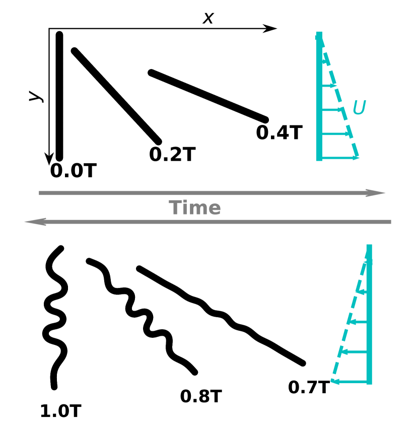
Figure 1: Sketch of our numerical experiment. Initially the filament is straight and is aligned vertically. The background shear flow, Equation (1) is shown as arrow: $t=T/4$ (top panel) and $t=3T/4$ (bottom panel).

Two effects determine the fate of an elastic filament in flow. One is the elastic nonlinearity of the filament and the other is the viscous interaction between the filament and the flow. The latter, in all its glory, gives rise to non–local and nonlinear interaction between two different parts of the same filament. Nevertheless, theoretical studies Doi and Edwards (1986); Goldstein and Langer (1995); Goldstein et al. (1998); Wolgemuth et al. (2000) have often approximated the viscous effect as a local, linear, isotropic drag. Can this local approximation to the flow–structure interaction still capture the shape chaos of a freely-floating filament ? As we show in the rest of this paper, the answer is yes; we prove shape chaos using Sharkovskii and Li and Yorke’s famous result Alligood et al. (1996) – existence of period orbits of period three implies not only the existence of orbits of all periods but also senstive dependence on initial condition.

In Figure. 1 we show a sketch of our numerical experiment. Initially the filament is aligned vertically. The background shear flow is given by

$${\bm{U}}_{0}(x,y)=\dot{\gamma}y\hat{\rm x}\/,\quad\text{and}\quad\dot{\gamma}=S\sin(\omega t)\/.$$ (1)

Here $T=2\pi/\omega$ is the time period of the periodic shear and $S$ is a constant.

II Model

We model the filament using the bead-spring model Larson et al. (1999); Guglielmini et al. (2012); Nazockdast et al. (2017); Slowicka et al. (2019); Wada and Netz (2006); Żuk et al. (2021): identical spherical beads of diameter $d$ are connected by over-damped springs of equilibrium length $a$. The position of the center of the $i$-th bead is $\bm{R}_{\rm i}$, where $i=1\ldots N$, the total number of beads. The equation of motion is:

$$\frac{\partial R^{\alpha}_{\rm i}}{\partial t}=-\frac{1}{3\pi\eta d}\frac{\partial\mathcal{H}}{\partial R^{\alpha}_{\rm i}}+U_{0}^{\alpha}(\bm{R}_{\rm i})\/,$$ (2)

where $U_{0}$ is given in (1). Here $\eta$ is viscosity of the fluid, $\partial(\cdot)/\partial(\cdot)$ denotes partial derivative, ${\bm{U}}_{0}$ is the velocity of the background shear, and $\mathcal{H}$ is the elastic Hamiltonian of the filament. The Greek indices run from 1 to $D$, the dimensionality of the space, and the Latin indices run from 1 to $N$. The elastic Hamiltonian Wada and Netz (2006, 2007), has contributions from bending ($\mathcal{H}_{\rm{B}}$) and stretching ($\mathcal{H}_{\rm{S}}$):

$$\mathcal{H} =\mathcal{H}_{\rm{B}}+\mathcal{H}_{\rm{S}}\quad\text{where}$$ (3a)

$$\mathcal{H}_{\rm B} =aB\sum_{{\rm i}=0}^{N-1}\kappa_{{\rm i}}^{2}\quad\text{and}$$ (3b)

$$\mathcal{H}_{\rm{S}} =\frac{H}{2a}\sum_{{\rm i}=0}^{N-1}\left(\lvert\bm{R}_{{\rm i}+1}-\bm{R}_{\rm i}\rvert-a\right)^{2}\/;\quad\text{where}$$ (3c)

$$\kappa_{\rm i} =\frac{1}{a}\lvert\hat{\bm{u}}_{\rm i}\times\hat{\bm{u}}_{{\rm i}-1}\rvert\/\quad\text{and}$$ (3d)

$$\hat{\bm{u}}_{\rm i} =\frac{\bm{R}_{{\rm i}+1}-\bm{R}_{\rm i}}{\lvert\bm{R}_{{\rm i}+1}-\bm{R}_{\rm i}\rvert}\/.$$ (3e)

Here $B$ is the bending modulus of the filament and $H$ is its stretching modulus. We ignore thermal fluctuations and torsion. Three dimensionless parameters determine the dynamics. We call them, the elasto–viscous parameters, the dimensionless frequency and the ratio of stretching to bending defined respectively as:

$$\overline{\mu} \equiv\frac{8\pi\eta SL^{4}}{B}\/,$$ (4a)

$$\sigma \equiv\frac{\omega}{S}\/,\quad\text{and}$$ (4b)

$$K \equiv\frac{Ha^{2}}{B}\/.$$ (4c)

In practice, the filaments are inextensible Powers (2010), which we implement by choosing appropriately high value of $K$. We evolve  Equation (2) using adaptive Runge-Kutta  Press and Teukolsky (1992) method with cash-karp parameters  Cash and Karp (1990). Our code is freely available  and has been benchmarked against experimental results Agrawal and Mitra (2022). A complete list of the parameters of the simulation is given in table 1. We study the problem for a large range of $\overline{\mu}$ and $\sigma$ all within experimentally realizable range. Note that, with the local approximation of viscous forces it is possible for the filament to cross itself. Such unphysical solutions do appear in our simulations but for values of $\overline{\mu}$ other than that has been considered in this paper. The computational complexity of the model, where the viscous interaction is modelled by the non–local Rotne–Pregor tensor Agrawal and Mitra (2022), is $\mathcal{O}(N^{2})$ where $N$ is the number of beads, whereas the computational complexity of the model with local viscosity is $\mathcal{O}(N)$. This allows us to run our simulations for much longer times than it was possible in Ref. Agrawal and Mitra (2022).

III Results

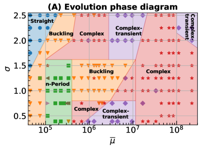
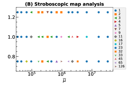
Figure 2: (A):Phase diagram in the $\overline{\mu}$–$\sigma$ plane; We find $5$ different qualitatively different dynamical phases: Straight($\bullet$); periodic ($\blacktriangledown$) with n-period, where n=2($\blacksquare$), 3($\blacktriangleleft$), 4($\blacktriangleright$); complex ($\bigstar$) complex-transients ($\blacklozenge$) (B) Solutions of stroboscopic map: The stroboscopic map has many periodic solutions at every point in $\overline{\mu}$–$\sigma$ plane. We show time period of the lowest cycle in Sharvoskii ordering.

A rigid ellipsoid in a periodic shear may show chaotic three–dimensional rotation under certain conditions Ramamohan et al. (1994); Kumar et al. (1995); Lundell (2011); Nilsen and Andersson (2013). Such behavior emerges due to the nonlinearities present in the Euler’s equations of rigid body rotation. Here we consider a filament with no inertia, hence such chaotic solutions are not present in our system. For a filament with high bending rigidity (small $\overline{\mu}$) we find that the filament merely translates and rotates coming back to its initial position and shape at the end of every period.

For a fixed dimensionless frequency ($\sigma$) as the bending rigidity is decreased ($\overline{\mu}$ is increased) an kaleidoscope of dynamic behavior emerges. We show an example in Figure. 1. During the first half-period the flow is extensional and the filament rotates. In the second half the flow is compressional and the filament can undergo buckling transition – the shape of the filament after one period is no longer straight but buckled. Furthermore, it may not come back to its initial position but may come back translated or rotated, neither of which are of interest to us in this paper – we focus on the shape of the filament. Under subsequent iterations of the periodic shear the buckled filament can go through many changes in shape.

We show a dynamic phase diagram in Fig. 2(A). Overall, at late times, the following possibilities exists:

1. The filament is always straight.

2. The filament reaches the same buckled shape at the end of each period.

3. The shape of the filament shows periodic behaviour with two-cycle, three-cycle, four-cycle, etc.

4. The shape of the filament is spatiotemporally chaotic. In Fig. 2(A) such solutions are marked complex.

5. The filament shows chaotic behavior for a long time but such behavior turns out to be transient. At late times the filament settles down to a complicated shape which changes very slowly. In Fig. 2(A) such solutions are marked complex transients.

We have observed the same qualitative behavior before Agrawal and Mitra (2022), for the case where the viscous forces are modeled by the non-local Rotne-Pregor tensor, with two crucial quantitative differences. We did not observe any three–period solution before and for large $\overline{\mu}$ we obtained complex transients for all values of $\sigma$ we used whereas here we observe the reappearance of the complex phase for the higher $\overline{\mu}$s. Nevertheless, we conclude that the model with local viscosity is able to capture the feature of the problem we consider essential – a rich dynamical phase diagram that includes complex shapes.

III.1 Stroboscopic map

The dynamical system described by (2) is non-autonomous because $\dot{\gamma}$ is an explicit function of time. Integrating (2) over exactly one time period $T$ gives us the position of every bead of the filament at $t=T$. Recall that the shape of the filament is fully specified by its curvature $\kappa$ as a function of arc length $s$. Thus we can define the stroboscopic map, $\mathcal{F}$, that allows us to obtain $\kappa(s,T)$ from $\kappa(s,0)$:

$$\kappa(s,T)=\mathcal{F}\kappa(s,0)\/.$$ (5)

The stroboscopic map is no longer an explicit function of time. Following Refs. Auerbach et al. (1987); Cvitanovic et al. (2005), we study the shape-chaos by obtaining the fixed points and periodic orbits of the stroboscopic map using the Newton–Krylov method, which is described in detail in appendix D1 of our earlier paper Agrawal and Mitra (2022). In general, for any fixed value of $\overline{\mu}$ and $\sigma$ we obtain many periodic orbits. We list all of them in table 2. We sort the cycles using Sharkovskiǐ’s ordering Sharkovski (1995):

$$3 \prec 5\prec 7\prec 9\prec 11\ldots\prec 2\cdot 3\prec 2\cdot 5\prec\ldots$$

$$\ldots \prec 2^{2}\cdot 3\prec 2^{2}\cdot 5\ldots\prec 2^{3}\cdot 3\prec 2^{3}\cdot 5\prec\ldots$$

$$\ldots \prec 2^{3}\prec 2^{2}\prec 2\prec 1\/,$$ (6)

In Fig. 2(B) we show the leading period of stroboscopic map, as it appears in Sharkovskii’s ordering, as a function of $\overline{\mu}$ and $\sigma$ – we do find orbits of period three. Although many periodic orbits appear as solutions of the map most of them are not stable and do not appear in the solution of dynamical equation. Let us recall the Sharkovskiǐ’s theorem Alligood et al. (1996): Consider a continuous map $f$ on an interval with a period $p$ orbit. If $p\prec q$, where $q$ appears in the Sharkovskiǐ’s ordering, then $f$ has a period-$q$ orbit. This implies that if $f$ possess a period $3$ orbit it has all orbits of all other periods. Although this shows that the map has very complex dynamical behavior it does not necessarily proves the existence of chaos. Nevertheless, existence of period three does imply chaos as was proved by Li and Yorke Li and Yorke (2004). Unfortunatley neither Sharkovskiǐ’s theorem nor the result of Li and Young is valid for maps in dimensions higher than unity Hence we conclude that although we demonstrate the rich complexity of the solutions of the stroboscopic map and we have not yet conclusively proven the existence of chaotic solutions.

III.2 Period three and the $\Theta$ map

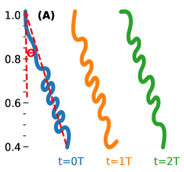
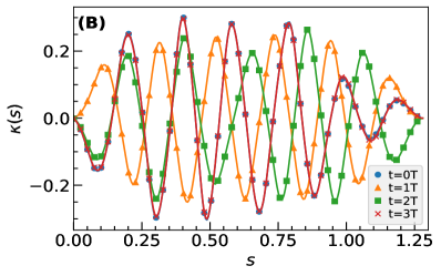
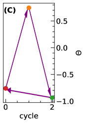
Figure 3: Example of a three period solution (for $\sigma=1,\overline{\mu}=1.67\times 10^{6}$) in real space (A) and curvature space (B) and for ($\sigma=0.75,\overline{\mu}=3.35\times 10^{5}$) in 1D $\Theta$-space (C). We start from $t=0$ and evolve the filament for three cycles. In (A,B), blue, orange and green curves shows the filament at $t=0,1T$, and $2T$ respectively. In (B), the $\kappa(s)$ plots for $t=0$ and $3T$ (blue, red) lie on top of each other.

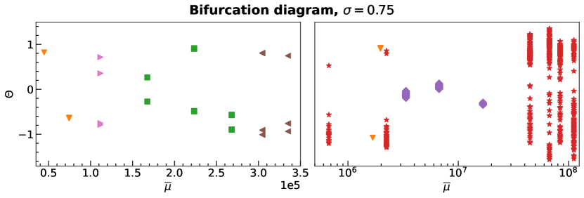
Figure 4: Bifurcation diagram of $\Theta$ for $\sigma=0.75$. The system shows chaos at high enough $\overline{\mu}$, except certain isolated ranges of $\overline{\mu}$, where $\Theta$ settles into periodic behavior – a behavior similar to island of order for bifurcation diagram of the logistic map Alligood et al. (1996).

The existence of period three solutions for both the evolution equations and the stroboscopic map is a key result in this problem. It behooves us to study it in greater detail. We choose the period-three solution that appears as a solution of stroboscopic map for $\sigma=1$ and $\overline{\mu}=1.6\times 10^{6}$. This is shown in Fig. 2(B) as a green triangle. In Fig. 3(A,B) we show the three solutions in real and curvature space respectively.

Now we attempt an arbitrary dimensional reduction to construct a one-dimensional map. We draw the straight line that connects the top end of the filament to the bottom one and call $\Theta$ the angle this line makes with the tangent to the filament at its top point, see Fig. 3(A). Defined this way, $\Theta$ does not depend on the position or orientation of the overall filament, but only its shape. In some cases, if shape of the filament shows a period three solution, so does $\Theta$. One such case is shown in Fig. 3(C) for $\sigma=0.75,\overline{\mu}=3.35\times 10^{5}$ . From the stroboscopic map we can construct a map for $\Theta$. This is a one dimensional map for which the Li and Yorke theorem is valid. Thus by demonstrating that the $\Theta$ map has three period we show that this map is chaotic. Further evidence of chaos is obtained by plotting the bifurcation diagram for $\Theta$ in Fig. 4. We find period two, period four and period three solutions and also chaotic ones.

III.3 Mixing of passive tracers

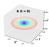
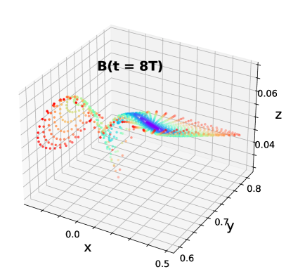
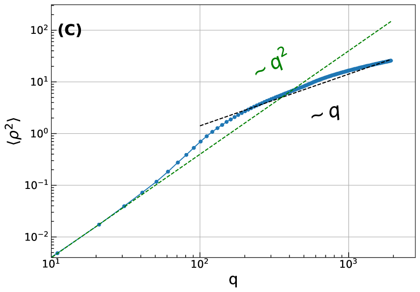
Figure 5: Mixing of passive tracer: (A) and (B) Positions of tracer particles at $t=0$ and $t=8T$. The parameters $\sigma=0.75$ and $\overline{\mu}=6.7\times 10^{7}$ are chosen such that we are in the complex phase. Initially, the tracers are placed on concentric circles, color coded by their distances from the center of the circles. The mixing of the colors show the mixing of the tracers. (C) Mean square displacement (MSD), $\left\langle\rho^{2}\right\rangle(qT)$, defined in (11), as a function of $q$ in log-log scale. We also plot two lines with slopes $1$ and $2$.

Next we demonstrate that if we choose $\overline{\mu}$ and $\sigma$ inside the complex phase, see Fig. 2(A), then the filament acts as an effective mixer of passive tracers. We use the same notation and technique used in our earlier paper Agrawal and Mitra (2022).

Once the filament has reached a statistically stationary state we introduce $N_{\rm p}$ tracers placed on concentric circles in the $x$–$y$ plane, Fig. 5(A). They are colored by radius of the circle on which they lie on at the initial time. For the rest of this section the time when the tracers are introduced is $t=0$. The equation of motion of the k-th tracer particle whose position at time $t$ is given by ${\bm{X}}^{{\rm k}}(t)$, is

$$\frac{d{\bm{X}}^{{\rm k}}}{dt}={\bm{U}}(\bm{r})\delta(\bm{r}-{\bm{X}}^{{\rm k}})\/.$$ (7)

Here ${\bm{U}}(\bm{r})$, the velocity of the flow at $\bm{r}=(x,y,z)$, is a superposition of the background flow velocity ${\bm{U}}_{0}(\bm{r})$ and the contributions from all the beads in the filament Rotne and Prager (1969); Brady and Bossis (1988); Guazzelli and Morris (2011); Kim and Karrila (2013):

$$U^{\alpha}(\bm{r}) =U_{0}^{\alpha}(\bm{r})+\mathcal{G}^{{\alpha\beta}}(\bm{r}-\bm{R}_{\rm i})F^{\beta}_{\rm i}\/,\quad\/,\text{where}$$ (8a)

$$F^{\alpha}_{\rm i} =-\frac{\partial\mathcal{H}}{\partial R^{\alpha}_{\rm i}}\/,\quad\text{and}$$ (8b)

$$\mathcal{G}^{{\alpha\beta}}(\bm{R}) =\frac{1}{8\pi\eta R}\left[\delta_{\alpha\beta}+\frac{R_{\alpha}R_{\beta}}{R^{2}}+\frac{d^{2}}{4R^{2}}\left(\frac{1}{3}\delta_{\alpha\beta}-\frac{R_{\alpha}R_{\beta}}{R^{2}}\right)\right]$$ (8c)

At $t=8T$, we find that most of the tracers have moved out of the plane and have become somewhat mixed, Fig. 5(B). At even later time, $t=128T$ (not shown), we find the tracer particles are well mixed. To obtain a quantitative measure of mixing we define

$$\Delta{\bm{X}}^{\rm k}_{\rm j}\equiv{\bm{X}}^{\rm k}((j+1)T)-{\bm{X}}^{\rm k}(jT)\quad\/,$$ (9)

the net displacement of the ${\rm k}$-th tracer particle over the $j$-th cycle – $t=jT$ to $t=(j+1)T$, where $j$ is an integer. The net displacement of the ${\rm k}$-th tracer after $q$ cycles is

$$\bm{\rho}^{{\rm k}}(q)=\sum_{j=1}^{q}\Delta{\bm{X}}^{{\rm k}}_{{\rm j}}\/.$$ (10)

The total mean square displacement, averaged over all the tracers, at the end of $q$ cycles is given by

$$\left\langle\rho^{2}(q)\right\rangle\equiv\frac{1}{N_{\rm p}}\sum_{{\rm k}=1}^{N_{\rm p}}\lvert\bm{\rho}^{{\rm k}}(q)\rvert^{2}$$ (11)

In Fig. 5(C) we plot $\left\langle\rho^{2}(q)\right\rangle$ versus $q$ in log-log scale. If the tracers diffuse then we expect $\left\langle\rho^{2}(q)\right\rangle\sim q$ for large $q$ Taylor (1922), which is what we obtain. Furthermore, we calculate the cumulative probability density function (CPDF) for each component of the displacement $\Delta{\bm{X}}^{{\rm k}}_{{\rm j}}$. For the out-of-plane component this CPDF has an exponential tail. For the in-plane components we obtain a power-law tail of exponent of $-3$. This implies that the probability density function (PDF) of each component of the displacement $\Delta{\bm{X}}^{{\rm k}}_{{\rm j}}$ is such that its second moment is well defined. Hence by the central limit theorem the probability density function of $\rho^{2}(q)$ is a Gaussian and we expect simple diffusive behavior. However, as the PDF (of displacement) has power-law tail we expect that very long averaging over very many number of tracer particles is necessary for convergence. This explains why we observe not-so-clear evidence of diffusion.

IV Conclusion

In this paper we consider a simplified model for a flexible filament in a viscous flow driven in a time–periodic manner. In particular, the simplicity lies is approximating the viscous forces by a local drag. We show that the shape of the filament is spatiotemporally chaotic. This model has only the elastic nonlinearity of the filament, hence it is solely the elastic nonlinearity that is responsible for chaos. This is the central message of this paper. An additional advantage of using the simplified model for viscous forces is that it may be possible to make theoretical progress following Goldstein and Langer Goldstein and Langer (1995).

The dimensionless parameters that we consider are within a range that is experimentally accessible. Although we do not expect exact quantitative agreement with experiment, We hope that, together with our previous work Agrawal and Mitra (2022), we have now presented convincing evidences that a single flexible filament in periodically driven Stokes flow can give chaotic solutions that is able to effectively mix passive scalars even at infinite Peclet number.

$N$	$256$
$a$	$0.005$
$d$	$0.005$
$L$	$1.28$
$B$	$6\times 10^{-6}\mbox{--}4\times 10^{-2}$
$S$	$2$
$\eta$	$10$
$\omega$	$1\mbox{--}6$
$\Delta$	$10^{-4}\mbox{--}10^{-6}$
$\overline{\mu}$	$12560\mbox{--}8.37\times 10^{7}$
$\sigma$	$0.5\mbox{--}3$
$K$	$16$

Table 1: Parameters of simulation: Number of beads, $N$, equilibrium distance between beads, $a$, bead diameter $d$, filament length $L$ Bending modulus $B$, viscosity $\eta$, time-step, $\Delta$. The quantities $S$ and $\omega$ defined in (1) determined the space-time dependence of the background flow. The dimensionless parameters $\overline{\mu}$, $\sigma$ and $K$ are defined in (4).

	0.75	1.0	1.25
$3.35\times 10^{4}$	1	1	1
$4.47\times 10^{4}$	1	1	1
$6.67\times 10^{4}$	1,16	1	1
$9.57\times 10^{4}$	1,4,20,22,23,27	2,4,11	1,2,3,12,13,24,25
$1.67\times 10^{5}$	1,2,10,14,33	1,2,3	1,2
$2.23\times 10^{5}$	1,2	1,2,3	1,2
$3.35\times 10^{5}$	1,2,3,4,5,7,9,10,15,19,22,23,31	1,2	1,2,7
$4.47\times 10^{5}$	1	1,2,3,5,6,7,13,19,37,41	1
$6.70\times 10^{5}$	1,2,5,7,12,25,32,41,47,50,68,76,85,100,104	1	1,2
$9.57\times 10^{5}$	1,126	1,4,9	1,2
$1.67\times 10^{6}$	1,50,54,62,65,66,70,80,86,108,132	1,2,3,4,5,7,9,22,44	1
$2.23\times 10^{6}$	1,11,12,28	1,2,45	1
$3.34\times 10^{6}$	1,2,4,32	1,4	1
$6.67\times 10^{6}$	$1^{\ast}$	1,17	1
$1.67\times 10^{7}$	$1^{\ast}$	$1^{\ast}$	$1^{\ast}$
$3.35\times 10^{7}$	$1^{\ast}$	$1^{\ast}$	$1^{\ast}$

Table 2: Cycles of the stroboscopic map. In some of these cases the evolution equation shows chaotic solution but so far we have obtained one or two periodic orbits of small periods, these are marked by $\ast$.

References

- Duprat (2022) C Duprat, “Moisture in textiles,” Annual Review of Fluid Mechanics 54, 443–467 (2022).
- Brennen and Winet (1977) Christopher Brennen and Howard Winet, “Fluid mechanics of propulsion by cilia and flagella,” Annual Review of Fluid Mechanics 9, 339–398 (1977).
- Sleigh (2016) Michael A Sleigh, The biology of Cilia and Flagella: international series of monographs on pure and applied biology: zoology, vol. 12, Vol. 12 (Elsevier, 2016).
- Du Roure et al. (2019) Olivia Du Roure, Anke Lindner, Ehssan N Nazockdast, and Michael J Shelley, “Dynamics of flexible fibers in viscous flows and fluids,” Annual Review of Fluid Mechanics 51, 539–572 (2019).
- Bruot and Cicuta (2016) Nicolas Bruot and Pietro Cicuta, “Realizing the physics of motile cilia synchronization with driven colloids,” Annual Review of Condensed Matter Physics 7, 323–348 (2016).
- Becker and Shelley (2001) Leif E Becker and Michael J Shelley, “Instability of elastic filaments in shear flow yields first-normal-stress differences,” Physical Review Letters 87, 198301 (2001).
- Guglielmini et al. (2012) Laura Guglielmini, Amit Kushwaha, Eric SG Shaqfeh, and Howard A Stone, “Buckling transitions of an elastic filament in a viscous stagnation point flow,” Physics of Fluids 24, 123601 (2012).
- Liu et al. (2018) Yanan Liu, Brato Chakrabarti, David Saintillan, Anke Lindner, and Olivia Du Roure, “Morphological transitions of elastic filaments in shear flow,” Proceedings of the National Academy of Sciences 115, 9438–9443 (2018).
- LaGrone et al. (2019) John LaGrone, Ricardo Cortez, Wen Yan, and Lisa Fauci, “Complex dynamics of long, flexible fibers in shear,” Journal of Non-Newtonian Fluid Mechanics 269, 73–81 (2019).
- Slowicka et al. (2019) AM Slowicka, Howard A Stone, and Maria L Ekiel-Jezewska, “Flexible fibers in shear flow: attracting periodic solutions,” arXiv preprint arXiv:1905.12985 (2019).
- Żuk et al. (2021) Paweł J Żuk, Agnieszka M Słowicka, Maria L Ekiel-Jeżewska, and Howard A Stone, “Universal features of the shape of elastic fibres in shear flow,” Journal of Fluid Mechanics 914 (2021).
- Kuei et al. (2015) Steve Kuei, Agnieszka M Słowicka, Maria L Ekiel-Jeżewska, Eligiusz Wajnryb, and Howard A Stone, “Dynamics and topology of a flexible chain: knots in steady shear flow,” New Journal of Physics 17, 053009 (2015).
- Hu et al. (2021) Shi-Yuan Hu, Jun-Jun Chu, Michael J Shelley, and Jun Zhang, “Lévy walks and path chaos in the dispersal of elongated structures moving across cellular vortical flows,” Physical Review Letters 127, 074503 (2021).
- Chakrabarti et al. (2020) Brato Chakrabarti, Yanan Liu, John LaGrone, Ricardo Cortez, Lisa Fauci, Olivia du Roure, David Saintillan, and Anke Lindner, “Flexible filaments buckle into helicoidal shapes in strong compressional flows,” Nature Physics , 1–6 (2020).
- Wiggins et al. (1998) Chris H Wiggins, D Riveline, Albrecht Ott, and Raymond E Goldstein, “Trapping and wiggling: elastohydrodynamics of driven microfilaments,” Biophysical journal 74, 1043–1060 (1998).
- Wolgemuth et al. (2000) Charles W Wolgemuth, Thomas R Powers, and Raymond E Goldstein, “Twirling and whirling: Viscous dynamics of rotating elastic filaments,” Physical Review Letters 84, 1623 (2000).
- Lim and Peskin (2004) Sookkyung Lim and Charles S Peskin, “Simulations of the whirling instability by the immersed boundary method,” SIAM Journal on Scientific Computing 25, 2066–2083 (2004).
- Wada and Netz (2006) Hirofumi Wada and Roland R Netz, “Non-equilibrium hydrodynamics of a rotating filament,” EPL (Europhysics Letters) 75, 645 (2006).
- Bonacci et al. (2022) Francesco Bonacci, Brato Chakrabarti, David Saintillan, Olivia du Roure, and Anke Lindner, “Dynamics of flexible filaments in oscillatory shear flows,” arXiv preprint arXiv:2205.08361 (2022).
- Agrawal and Mitra (2022) Vipin Agrawal and Dhrubaditya Mitra, “Chaos and irreversibility of a flexible filament in periodically driven stokes flow,” Physical Review E 106, 025103 (2022).
- Krishnamurthy and Prakash (2022) Deepak Krishnamurthy and Manu Prakash, “Emergent programmable behavior and chaos in dynamically driven active filaments,” bioRxiv (2022).
- Doi and Edwards (1986) M Doi and SF Edwards, “The theory of polymer dynamics,” (1986).
- Goldstein and Langer (1995) Raymond E Goldstein and Stephen A Langer, “Nonlinear dynamics of stiff polymers,” Physical review letters 75, 1094 (1995).
- Goldstein et al. (1998) Raymond E Goldstein, Thomas R Powers, and Chris H Wiggins, “Viscous nonlinear dynamics of twist and writhe,” Physical Review Letters 80, 5232 (1998).
- Alligood et al. (1996) Kathleen T Alligood, Tim D Sauer, and James A Yorke, Chaos: An introduction to dynamical systems (Springer, New York, 1996).
- Larson et al. (1999) RG Larson, Hua Hu, DE Smith, and S Chu, “Brownian dynamics simulations of a dna molecule in an extensional flow field,” Journal of Rheology 43, 267–304 (1999).
- Nazockdast et al. (2017) Ehssan Nazockdast, Abtin Rahimian, Denis Zorin, and Michael Shelley, “A fast platform for simulating semi-flexible fiber suspensions applied to cell mechanics,” Journal of Computational Physics 329, 173–209 (2017).
- Wada and Netz (2007) Hirofumi Wada and Roland R Netz, “Stretching helical nano-springs at finite temperature,” EPL (Europhysics Letters) 77, 68001 (2007).
- Powers (2010) Thomas R Powers, “Dynamics of filaments and membranes in a viscous fluid,” Reviews of Modern Physics 82, 1607 (2010).
- Press and Teukolsky (1992) William H Press and Saul A Teukolsky, “Adaptive stepsize runge-kutta integration,” Computers in Physics 6, 188–191 (1992).
- Cash and Karp (1990) Jeff R Cash and Alan H Karp, “A variable order runge-kutta method for initial value problems with rapidly varying right-hand sides,” ACM Transactions on Mathematical Software (TOMS) 16, 201–222 (1990).
- Note (1) https://github.com/dhrubaditya/ElasticString.
- Ramamohan et al. (1994) TR Ramamohan, S Savithri, R Sreenivasan, and C Chandra Shekara Bhat, “Chaotic dynamics of a periodically forced slender body in a simple shear flow,” Physics Letters A 190, 273–278 (1994).
- Kumar et al. (1995) CV Kumar, K Satheesh Kumar, and TR Ramamohan, “Chaotic dynamics of periodically forced spheroids in simple shear flow with potential application to particle separation,” Rheologica acta 34, 504–511 (1995).
- Lundell (2011) Fredrik Lundell, “The effect of particle inertia on triaxial ellipsoids in creeping shear: from drift toward chaos to a single periodic solution,” Physics of Fluids 23, 011704 (2011).
- Nilsen and Andersson (2013) Christopher Nilsen and Helge I Andersson, “Chaotic rotation of inertial spheroids in oscillating shear flow,” Physics of Fluids 25, 013303 (2013).
- Auerbach et al. (1987) Ditza Auerbach, Predrag Cvitanović, Jean-Pierre Eckmann, Gemunu Gunaratne, and Itamar Procaccia, “Exploring chaotic motion through periodic orbits,” Physical Review Letters 58, 2387 (1987).
- Cvitanovic et al. (2005) Predrag Cvitanovic, Roberto Artuso, Ronnie Mainieri, Gregor Tanner, Gábor Vattay, Niall Whelan, and Andreas Wirzba, “Chaos: classical and quantum,” ChaosBook. org (Niels Bohr Institute, Copenhagen 2005) 69, 25 (2005).
- Sharkovski (1995) AN Sharkovski, “Coexistence of cycles of a continuous map of the line into itself,” International journal of bifurcation and chaos 5, 1263–1273 (1995).
- Li and Yorke (2004) Tien-Yien Li and James A Yorke, “Period three implies chaos,” in The theory of chaotic attractors (Springer, 2004) pp. 77–84.
- Note (2) As a counterexample Kloeden and Li (2006), consider the two dimensional map that rotates every point in the plane by an angle of in the counter-clockwise direction. Clearly this map has a period three solution but it is not chaotic.
- Note (3) It is also possible that the shape shows period three solution but the shows a fixed point or a period–two solution. Conversely, it is possible for to have a period–three solution without the shape having a period-three solution.
- Rotne and Prager (1969) Jens Rotne and Stephen Prager, “Variational treatment of hydrodynamic interaction in polymers,” The Journal of Chemical Physics 50, 4831–4837 (1969).
- Brady and Bossis (1988) John F Brady and Georges Bossis, “Stokesian dynamics,” Annual review of fluid mechanics 20, 111–157 (1988).
- Guazzelli and Morris (2011) Elisabeth Guazzelli and Jeffrey F Morris, A physical introduction to suspension dynamics, Vol. 45 (Cambridge University Press, 2011).
- Kim and Karrila (2013) Sangtae Kim and Seppo J Karrila, Microhydrodynamics: principles and selected applications (Courier Corporation, 2013).
- Taylor (1922) Geoffrey I Taylor, “Diffusion by continuous movements,” Proceedings of the london mathematical society 2, 196–212 (1922).
- Kloeden and Li (2006) Peter Kloeden and Zhong Li, “Li–yorke chaos in higher dimensions: A review,” Journal of Difference Equations and Applications 12, 247–269 (2006).