Braid variety cluster structures, I: 3D plabic graphs

Résumé.

We introduce $3$-dimensional generalizations of Postnikov’s plabic graphs and use them to establish cluster structures for type $A$ braid varieties. Our results include known cluster structures on open positroid varieties and double Bruhat cells, and establish new cluster structures for type $A$ open Richardson varieties.

1. Introduction

Braid varieties $\accentset{\circ}{R}_{{u,\beta}}$ are smooth, affine, complex algebraic varieties associated to a permutation $u$ and a braid word $\beta$, that is, a word representing an element of the positive braid monoid. The purpose of this work is to construct a cluster algebra structure [FZ02] on the coordinate ring of a braid variety.

Theorem 1.1.

The coordinate ring ${\mathbb{C}}[\accentset{\circ}{R}_{u,\beta}]$ of a braid variety is a cluster algebra.

The braid varieties we consider were studied, rather recently, in [Mel19, CGGS20], generalizing varieties considered previously in [Deo85, MR04, WY07]. Theorem 1.1 resolves conjectures of [Lec16, CGGS21].

Certain special cases of braid varieties, namely open Richardson varieties and open positroid varieties, have played a key role in the combinatorial geometry of flag varieties and Grassmannians. Open Richardson varieties $\accentset{\circ}{R}_{u,w}$ are subvarieties of the variety $\operatorname{SL}_{n}/B_{+}$ of complete flags in ${\mathbb{C}}^{n}$, arising in the study of total positivity and Poisson geometry [Deo85, Lus98, MR04, Pos06, BGY06, KLS13]. An explicit cluster structure for open Richardson varieties was conjectured by Leclerc [Lec16]. Ménard [Mé22] gave an alternative conjectural cluster structure, which was proved by Cao and Keller [CK22] to be an upper cluster structure; Ménard’s and Leclerc’s cluster structures are expected to coincide. Another upper cluster structure was constructed by Ingermanson [Ing19]. The cluster structure of Theorem 1.1, in the case of open Richardson varieties, agrees with that of Ingermanson. It is related to the cluster structure of Leclerc [Lec16] by the twist automorphism [GL22b, SSB].

We also prove that the cluster varieties in Theorem 1.1 are locally acyclic [Mul13]; in the case of open Richardson varieties we use this to establish a variant of a conjecture of Lam and Speyer [LS16]. In particular, the cohomology of braid varieties satisfies the curious Lefschetz phenomenon (Theorem 10.1).

Theorem 1.1 generalizes the (type A) results of [FZ99, GY20] on double Bruhat cells and [SW21] on double Bott–Samelson cells, and also the results of Ingermanson [Ing19] and Cao and Keller [CK22], who found upper cluster structures on open Richardson varieties (see also [Mé22]). Furthermore, Theorem 1.1 generalizes the main result of [GL19] (see also [Sco06, MS16, SSBW19]), where the same statement was proved for open positroid varieties [KLS13], which are special cases of open Richardson varieties. Positroid varieties are parametrized by plabic graphs [Pos06], whose planar dual quivers describe the cluster algebra structure on the associated open positroid varieties.

Ever since the completion of [GL19], it has been our hope that constructing a cluster structure for open Richardson varieties would lead to a meaningful generalization of Postnikov’s plabic graphs; indeed, discovering such a generalization turned out to be a crucial step in our proof of Theorem 1.1. We associate a 3D plabic graph to each pair $(u,\beta)$ consisting of a permutation $u$ and a (double) braid word $\beta$, and use the combinatorics of this graph to construct our cluster structure. The reader is invited to look forward at the examples in Figures 1–5.

An important geometric ingredient in our approach is the study of the Deodhar geometry of braid varieties, originally used by Deodhar [Deo85] in the flag variety setting. We define an open Deodhar torus $T_{u,\beta}\subset\accentset{\circ}{R}_{u,\beta}$, and our cluster variables are interpreted as characters of $T_{u,\beta}$ that have certain orders of vanishing along the Deodhar hypersurfaces in the complement of the Deodhar torus. We expect this geometric approach to have applications to other settings where cluster structures are expected to make an appearance.

Our work has a number of applications. Our cluster structure implies, via [LS16], a curious Lefschetz phenomenon for the cohomology of braid varieties. Our approach is closely related to the combinatorics of braid Richardson links that are associated to a braid variety; in particular, we relate certain quiver point counts to the HOMFLY polynomial of these links.

We learned at the final stages of completing this manuscript that a cluster structure for braid varieties was independently announced in a recent preprint [CGG⁺22]. It would be interesting to investigate the relation between our 3D plabic graphs and the approach of [CGG⁺22]. The results of [CGG⁺22] apply more generally to braid varieties of arbitrary Lie type, while in the present paper we focus on varieties of type $A$. Our results and methods will be extended to include braid varieties of arbitrary type in a separate paper [GLSBS].

Overview

In Section 2, we give a synopsis of our main results in the setting of open Richardson varieties. In the rest of the paper we work in the setting of braid varieties. We define 3D plabic graphs and the associated quivers $\widetilde{Q}_{u,\beta}$ in Section 3. Next, we develop the combinatorics of 3D plabic graphs and show that the quivers $\widetilde{Q}_{u,\beta}$ are invariant under braid moves on the word $\beta$, naturally extending square moves from Postnikov’s plabic graphs to 3D plabic graphs; see Section 4. We discuss cluster algebras associated to 3D plabic graphs in Section 5 and show that they are locally acyclic in the sense of [Mul13]. In Sections 6 and 7, we study the Deodhar geometry of $\accentset{\circ}{R}_{{u,\beta}}$ and construct a seed in ${\mathbb{C}}(\accentset{\circ}{R}_{{u,\beta}})$ for each 3D plabic graph. We then show that the seeds are related by mutation in Section 8. Finally, in Section 9, we prove Theorem 7.14 by induction on the length of $\beta$. We conclude with some applications of our approach in Section 10.

Acknowledgments

T.L. and D.E.S. thank our students Ray Karpman and Gracie Ingermanson for helping us understand the relationship between Deodhar’s positive subexpressions and Postnikov’s combinatorics and for the other ideas discussed in Section 2.6. M.S.B. thanks Daping Weng for illuminating conversations on [SW21]. We also appreciate many conversations with Allen Knutson about Richardson and Bott–Samelson varieties, and Deodhar tori. We thank Roger Casals, Eugene Gorsky, and Anton Mellit for conversations related to this project. We also thank the authors of [CGG⁺22] for sharing their exciting results with us.

2. Open Richardson varieties

In this section, we give a more detailed explanation of Theorem 1.1 in the case of open Richardson varieties.

2.1. Open Richardson varieties

Let $G=\operatorname{SL}_{n}$, and let $B_{+}$, $B_{-}$ be the opposite Borel subgroups of upper and lower triangular matrices, respectively. For two permutations $u,w\in S_{n}$ such that $u\leq w$ in the Bruhat order, the open Richardson variety $\accentset{\circ}{R}_{u,w}$ is defined as

$$\accentset{\circ}{R}_{u,w}:=(B_{-}uB_{+}\cap B_{+}wB_{+})/B_{+}.$$

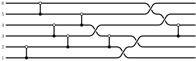
Figure 1. A 3D plabic graph $G_{u,{\mathbf{w}}}$.

To each pair $u\leq w$ and to each reduced word ${\mathbf{w}}$ for $w$ we associate an ice quiver $\widetilde{Q}_{u,{\mathbf{w}}}$ (Section 2.3). Let $\mathcal{A}(\widetilde{Q}_{u,{\mathbf{w}}})$ be the associated cluster algebra; see Section 5.1 for background.

Theorem 2.1.

For all $u\leq w$ in $S_{n}$, we have an isomorphism

$${\mathbb{C}}[\accentset{\circ}{R}_{u,w}]\cong\mathcal{A}(\widetilde{Q}_{u,{\mathbf{w}}}).$$

Moreover, the cluster algebra $\mathcal{A}(\widetilde{Q}_{u,{\mathbf{w}}})$ is locally acyclic and really full rank.

The cluster algebra terminology in Theorem 2.1 will be introduced in Section 5.1. We now describe the 3D plabic graph $G_{u,{\mathbf{w}}}$, the quiver $\widetilde{Q}_{u,{\mathbf{w}}}$, and the associated cluster algebra $\mathcal{A}(\widetilde{Q}_{u,{\mathbf{w}}})$.

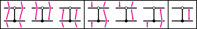
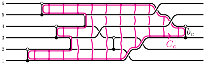
Figure 2. Propagation rules (right to left) for the relative cycles in $G_{u,{\mathbf{w}}}$.

Figure 3. Applying propagation rules to find one relative cycle $C_{c}$ of $G_{u,{\mathbf{w}}}$.

2.2. 3D plabic graphs

Let ${\mathbf{w}}=(i_{1},i_{2},\dots,i_{m})$ be a reduced word for $w$. Consider the unique rightmost subexpression ${\mathbf{u}}$ for $u$ inside ${\mathbf{w}}$, and let $J_{u,{\mathbf{w}}}\subset[m]:=\{1,2,\dots,m\}$ be the set of indices not used in ${\mathbf{u}}$. The 3D plabic graph $G_{u,{\mathbf{w}}}$ is obtained from the wiring diagram for $w$ by replacing all crossings in $[m]\setminus J_{u,{\mathbf{w}}}$ by overcrossings and replacing each crossing $c\in J_{u,{\mathbf{w}}}$ by a black-white bridge edge $b_{c}$; see Figure 1. We place a marked point on each of the $n$ leftmost boundary vertices of $G_{u,{\mathbf{w}}}$, and denote by $\mathbf{M}$ the set of these marked points.

The number of bridges in $G_{u,{\mathbf{w}}}$ is $|J_{u,{\mathbf{w}}}|=\ell(w)-\ell(u)$, which is the dimension of $\accentset{\circ}{R}_{u,w}$. To each index $c\in J_{u,{\mathbf{w}}}$ we will associate an (oriented) relative cycle $C_{c}$ in $G_{u,{\mathbf{w}}}$, which by definition is either a cycle in $G_{u,{\mathbf{w}}}$ or a union of oriented paths in $G_{u,{\mathbf{w}}}$ with endpoints in $\mathbf{M}$.

Each relative cycle $C_{c}$ will naturally bound a disk $D_{c}$. For instance, in Figure 3, the vertical sections of $D_{c}$ are shown in wavy pink lines. We indicate the relative position of $D_{c}$ in ${\mathbb{R}}^{3}$ with respect to the edges of $G_{u,{\mathbf{w}}}$ by over/under-crossings. We will compute $D_{c}$, and therefore its boundary $C_{c}$, starting from the bridge $b_{c}$ and proceeding to the left using the propagation rules in Figure 3. We choose the counterclockwise orientation of $C_{c}$, so that as one traverses $C_{c}$, the disk $D_{c}$ is to the left. See Section 3.4 for a description of relative cycles in the case of double braid varieties.

2.3. The quiver

A quiver $Q$ is a directed graph without directed cycles of length $1$ and $2$. An ice quiver $\widetilde{Q}$ is a quiver whose vertex set $\widetilde{V}=V(\widetilde{Q})$ is partitioned into frozen and mutable vertices: $\widetilde{V}=V^{\operatorname{fro}}\sqcup V^{\operatorname{mut}}$. The arrows between pairs of frozen vertices are automatically omitted.

The procedure in Section 2.2 yields a bicolored graph $G_{u,{\mathbf{w}}}$ decorated with a family $(C_{c})_{c\in J_{u,{\mathbf{w}}}}$ of relative cycles. To this data, we associate an ice quiver $\widetilde{Q}_{u,{\mathbf{w}}}$. Our construction will rely on the results of [FG09, GK13]. The vertex set $V(\widetilde{Q}_{u,{\mathbf{w}}}):=J_{u,{\mathbf{w}}}$ is in bijection with the set of relative cycles. If a relative cycle $C_{c}$ is actually a cycle in $G_{u,{\mathbf{w}}}$ then $c$ is a mutable vertex of $\widetilde{Q}_{u,{\mathbf{w}}}$; otherwise, if $C_{c}$ is a union of paths with endpoints in $\mathbf{M}$, $c$ is a frozen vertex of $\widetilde{Q}_{u,{\mathbf{w}}}$.

To compute the arrows of $\widetilde{Q}_{u,{\mathbf{w}}}$, we consider $G_{u,{\mathbf{w}}}$ as a ribbon graph, with counterclockwise half-edge orientations around white vertices and clockwise half-edge orientations around black vertices. Let $\mathbf{S}_{u,{\mathbf{w}}}$ be the surface with boundary obtained by replacing every edge of $G_{u,{\mathbf{w}}}$ by a thin ribbon and gluing the ribbons together according to the local orientations at the vertices of $G_{u,{\mathbf{w}}}$. See Figure 6(d) for an example of $\mathbf{S}_{u,{\mathbf{w}}}$. The $n$ marked points of $G_{u,{\mathbf{w}}}$ give rise to $n$ marked points on $\partial\mathbf{S}_{u,{\mathbf{w}}}$, the set of which is also denoted by $\mathbf{M}$.

We view each relative cycle $C_{c}$ as an element of the relative homology $\Lambda_{u,{\mathbf{w}}}:=H_{1}(\mathbf{S}_{u,{\mathbf{w}}},\mathbf{M})$. It turns out that each mutable relative cycle can be also viewed as an element of the dual lattice $\Lambda^{\ast}_{u,{\mathbf{w}}}$; see Section 3.3. The (signed) number of arrows between two vertices $c,d\in J_{u,{\mathbf{w}}}$ in $\widetilde{Q}_{u,{\mathbf{w}}}$, where $d$ is mutable, is defined to be the (signed) intersection number ${\langle}C_{c},C_{d}{\rangle}$ of the relative cycles $C_{c}$ and $C_{d}$. These intersection numbers can be computed explicitly using simple pictorial rules; see Algorithm 3.8.

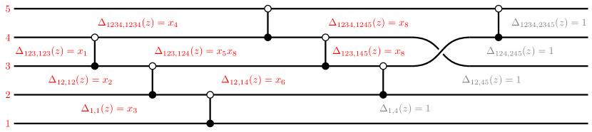
Figure 4. Factorization of chamber minors into cluster variables.

2.4. The seed

To each $c\in J_{u,{\mathbf{w}}}$ we associate a cluster variable $x_{c}\in{\mathbb{C}}[\accentset{\circ}{R}_{u,w}]$. Let $\mathbf{Ch}_{c}$ be the chamber (i.e., a connected component of the complement of $G_{u,{\mathbf{w}}}$ in the plane) located immediately to the left of the bridge $b_{c}$. To this data, one can associate a regular function on $\accentset{\circ}{R}_{u,w}$ called a chamber minor $\Delta_{c}\in{\mathbb{C}}[\accentset{\circ}{R}_{u,w}]$. Variants of these functions appear in [MR04, Lec16, Ing19].

Specifically, given an element $gB_{+}\in\accentset{\circ}{R}_{u,w}$, one can find a unique matrix $z\in B_{+}$ such that $gB_{+}=zwB_{+}$ and $\Delta_{u[i],w[i]}(z)=1$ for all $i=1,2,\dots,n$. Here we write $v[i]:=\{v(1),\dots,v(i)\}$ for $v\in S_{n}$, and $\Delta_{A,B}$ denotes the matrix minor with row set $A$ and column set $B$. The wiring diagram of $w$ is obtained from $G_{u,{\mathbf{w}}}$ by replacing every bridge with a crossing, and the wiring diagram of $u$ is obtained by erasing all bridges from $G_{u,{\mathbf{w}}}$. Given any chamber $\mathbf{Ch}$, let $A$ be the set of left endpoints of $u$-strands (i.e., the strands in the wiring diagram of $u$) passing below $\mathbf{Ch}$, and let $B$ be the set of left endpoints of $w$-strands passing below $\mathbf{Ch}$. The chamber minor for $\mathbf{Ch}$ is then given by $\Delta_{A,B}(z)$.

For $d\in J_{u,{\mathbf{w}}}$, we say that $\mathbf{Ch}_{c}$ is inside $C_{d}$ if it is contained inside the projection of the disk $D_{d}$ to the plane. Then the cluster variables $(x_{c})_{c\in J_{u,{\mathbf{w}}}}$ are uniquely defined by the invertible monomial transformation

(2.1) $$\Delta_{c}=\prod_{d\in J_{u,{\mathbf{w}}}:\ \text{$\mathbf{Ch}_{c}$ is inside $C_{d}$}}x_{d}.$$

See Figure 4 for an example when $w=s_{3}s_{2}s_{1}s_{4}s_{3}s_{2}s_{3}s_{4}$ and $u=s_{3}$, and see Section 6.6.1 for further details.

The cluster $\{x_{c}\}_{c\in J_{u,{\mathbf{w}}}}$ together with the quiver $\widetilde{Q}_{u,{\mathbf{w}}}$ is a seed $\Sigma_{u,{\mathbf{w}}}$ in ${\mathbb{C}}(\accentset{\circ}{R}_{u,w})$. To prove Theorem 2.1, we show that ${\mathbb{C}}[\accentset{\circ}{R}_{u,w}]={\mathcal{A}}(\Sigma_{u,{\mathbf{w}}})$.

2.5. Deodhar geometry

In [Deo85], Deodhar constructed a stratification of $\accentset{\circ}{R}_{u,w}$ for each reduced word ${\mathbf{w}}$ of $w$. The strata are of the form ${\mathbb{C}}^{a}\times({\mathbb{C}}^{*})^{b}$. The dense open stratum in Deodhar’s stratification is called the Deodhar torus, and denoted $T_{u,{\mathbf{w}}}\subset\accentset{\circ}{R}_{u,w}$. The Deodhar torus is the initial cluster torus in our cluster structure. We show in Proposition 7.4 that the chamber minors $\{\Delta_{c}\}_{c\in J_{u,{\mathbf{w}}}}$ are a basis of characters for $T_{u,{\mathbf{w}}}$.

We show that the cluster variables $\{x_{d}\}_{d\in J_{u,{\mathbf{w}}}}$ are certain distinguished characters on $T_{u,{\mathbf{w}}}$. Namely, the complement $\accentset{\circ}{R}_{u,w}\setminus T_{u,{\mathbf{w}}}$ is a union of irreducible components called (mutable) Deodhar hypersurfaces $V_{d}$. We deduce from (2.1) that the mutable cluster variable $x_{d}$ is the unique character of $T_{u,{\mathbf{w}}}$ which vanishes to order one along $V_{d}$ and has no zeroes along other Deodhar hypersurfaces. Frozen Deodhar hypersurfaces and frozen cluster variables are constructed using a slightly different geometric approach.

2.6. Comparison to known cluster structures

Our construction simultaneously includes several known cluster structures.

When $w$ is a $k$-Grassmannian permutation, the open Richardson variety $\accentset{\circ}{R}_{u,w}$ is an open positroid variety in the sense of [Pos06, KLS13]. In this case, Karpman [Kar17] showed that the graph $G_{u,{\mathbf{w}}}$ is one of Postnikov’s reduced plabic graphs [Pos06] with $n$ extra leaves attached. In particular, in this case $G_{u,{\mathbf{w}}}$ is planar and each cycle $C_{c}$ bounds a single face of $G_{u,{\mathbf{w}}}$, which is not usually true for general $w\in S_{n}$. In this case, the first two authors [GL19] showed that the open positroid variety is a cluster variety, with quiver coming from the plabic graph; this gives the quiver $\widetilde{Q}_{u,{\mathbf{w}}}$.

Many of our ideas appeared in the unpublished Ph.D. dissertation of Ingermanson [Ing19], which constructs an upper cluster structure on $\accentset{\circ}{R}_{u,w}$. The fourth author was Ingermanson’s advisor and is grateful for the ideas he learned from her. We summarize the constructions in our paper that appear in [Ing19]. Ingermanson writes down the same monomial transformation as (2.1), but defines it via a much more involved recursion. Ingermanson constructs a bridge diagram (in the case that ${\mathbf{w}}$ is a particular reduced word called the “unipeak word”) which is isomorphic to our graph $G_{u,{\mathbf{w}}}$ but is defined as an abstract graph rather than embedded in ${\mathbb{R}}^{3}$. Ingermanson’s quiver is identical to our $\widetilde{Q}_{u,{\mathbf{w}}}$, but it is described in a very different way, along the lines of Section 3.7.

2.7. Braid Richardson varieties

Open Richardson varieties generalize to braid Richardson varieties. We say that two flags $B_{1},B_{2}\in G/B_{+}$ are in relative position $w\in S_{n}$ if there exists a matrix $g\in G$ such that $(gB_{1},gB_{2})=(B_{+},wB_{+})$. In this case, we write $B_{1}\stackrel{{\scriptstyle w}}{{\longrightarrow}}B_{2}$. Consider a (not necessarily reduced) word $\beta=(i_{1},i_{2},\dots,i_{m})\in[n-1]^{m}$ and let $u\in S_{n}$. Following the nomenclature of [GLTW22], define the braid Richardson variety

(2.2) $$\accentset{\circ}{R}_{u,\beta}=\left\{(B_{1},B_{2},\dots,B_{m})\in(G/B_{+})^{m}\mid B_{+}\xrightarrow{s_{i_{1}}}B_{1}\xrightarrow{s_{i_{2}}}\cdots\xrightarrow{s_{i_{m}}}B_{m}\xleftarrow{w_{0}u}B_{-}\right\}.$$

This variety is nonempty whenever $u\leq\beta$ in the sense of Definition 3.1. In the case $u=w_{0}$, the definition (2.2) is the same as the definition of the braid variety $X(\beta)$ considered in [CGG⁺22], and is isomorphic to the braid variety $X(\beta,w_{0})$ in [CGGS20]. We shall show that braid Richardson varieties are isomorphic to the braid varieties we study in Section 6.

When $\beta$ is a reduced word for some $w\in S_{n}$ then using a variant of Lemma 6.2(2–3), we see that $\accentset{\circ}{R}_{u,\beta}$ is isomorphic to the space $\left\{B\in G/B_{+}\mid B_{+}\xrightarrow{w}B\xleftarrow{w_{0}u}B_{-}\right\}$ which can be identified with the Richardson variety $\accentset{\circ}{R}_{u,w}\subset G/B_{+}$. Thus, braid Richardson varieties generalize open Richardson varieties. Theorem 2.1 extends to the setting of braid Richardson varieties.

In Section 3.1, we describe our construction in the most general setting of double braid varieties, and define a 3D plabic graph $G_{u,\beta}$ and a quiver $\widetilde{Q}_{u,\beta}$ for a pair $(u,\beta)$ consisting of a permutation $u$ and a double braid word $\beta$ (Section 3.1). If $\beta$ is a double braid word and $u={\operatorname{id}}$, then $G_{u,\beta}$ is again planar. In this case, if we impose that the double word $\beta$ is reduced, we recover the classical cluster structure on type A double Bruhat cells [FZ99, BFZ05, GY20]. If we allow $\beta$ to be non-reduced, then we recover the type A results of [SW21] on double Bott–Samelson varieties. We note that the fact that our graphs are non-planar indicates that our construction gives a non-trivial $3$-dimensional extension of the combinatorics of [FZ99, Pos06, SW21].

3. Double braid quivers

The goal of this section is to define 3D plabic graphs, conjugate surfaces, relative cycles, and the associated quivers in the extended generality of double braid words.

3.1. Double braid words

Let $I:=[n-1]$. A double braid word is a word $\beta=(i_{1},i_{2},\dots,i_{m})\in(\pm I)^{m}$ in the alphabet

$$\pm I:=\{-1,-2,\dots,-(n-1)\}\sqcup\{1,2,\dots,n-1\}.$$

We denote the set of double braid words by $(\pm I)^{m}$. We will usually abbreviate $\beta=(i_{1},i_{2},\dots,i_{m})$ as $\beta=i_{1}i_{2}\dots i_{m}$. For $\beta\in(\pm I)^{m}$, we write $\ell(\beta):=m$. The goal of this section is to associate a quiver $\widetilde{Q}_{u,\beta}$ to a pair $(u,\beta)$, where $u\in S_{n}$ and $\beta\in(\pm I)^{m}$.

The word $\beta\in(\pm I)^{m}$ should be considered as a shuffle of two positive braid words in the commuting alphabets $I,-I$. We emphasize that the letter $-i$ does not correspond to $\sigma_{i}^{-1}$, the inverse of the braid group generator $\sigma_{i}$. We call elements of $I$ red and elements of $-I$ blue.

For $i\in\pm I$, let

$$s_{i}^{+}:=\begin{cases}s_{i},&\text{if }i>0,\\ {\operatorname{id}},&\text{if }i<0,\end{cases}\quad s_{i}^{-}:=\begin{cases}{\operatorname{id}},&\text{if }i>0,\\ s_{-i},&\text{if }i<0.\\ \end{cases}$$

We use the convention that the positive indices act on the right while the negative indices act on the left; for a permutation $u\in S_{n}$ and $i\in\pm I$, we write this action as $u\mapsto s_{i}^{-}us_{i}^{+}$. For a double braid word $\beta$, its Demazure product is defined by

$$\pi(\beta):=s_{i_{m}}^{-}*s_{i_{m-1}}^{-}*\cdots*s_{i_{1}}^{-}*s_{i_{1}}^{+}*s_{i_{2}}^{+}*\cdots*s_{i_{m}}^{+}\quad\in S_{n},$$

where $*$ denotes the standard Demazure product on $S_{n}$.

Definition 3.1.

For $u\in S_{n}$ and a double braid word $\beta$, we write $u\leq\beta$ if $u\leq\pi(\beta)$ in the Bruhat order on $S_{n}$.

Let $\beta=(i_{1},i_{2},\dots,i_{m})\in(\pm I)^{m}$ and $u\in S_{n}$. A $u$-subexpression of $\beta$ is a sequence ${\mathbf{u}}=(u_{(0)},u_{(1)},\dots,u_{(m)})\in S_{n}^{m+1}$ such that $u_{(0)}={\operatorname{id}}$, $u_{(m)}=u$, and such that for each $c\in[m]$, we have either $u_{(c)}=u_{(c-1)}$ or $u_{(c)}=s_{i_{c}}^{-}u_{(c-1)}s_{i_{c}}^{+}$. It is clear that $\beta$ contains a $u$-subexpression if and only if $u\leq\beta$.

Suppose that $u\leq\beta$. Out of all $u$-subexpressions of $\beta$, there exists a unique “rightmost” one, called the $u$-positive distinguished subexpression ($u$-PDS). It can be computed explicitly using the following operation which we call Demazure quotient: for $u\in S_{n}$ and $i\in I$, set

$$s_{i}\vartriangleright u=\begin{cases}s_{i}u,&\text{ if }s_{i}u<u,\\ u,&\text{otherwise,}\end{cases}\quad\text{and}\quad u\vartriangleleft s_{i}=\begin{cases}us_{i},&\text{ if }us_{i}<u,\\ u,&\text{otherwise.}\end{cases}$$

By convention, we set ${\operatorname{id}}\vartriangleright u=u=u\vartriangleleft{\operatorname{id}}$. The $u$-PDS ${\mathbf{u}}=(u_{(0)},u_{(1)},\dots,u_{(m)})$ is computed iteratively starting from $u_{(m)}=u$. For $c=m,m-1,\dots,1$, we set

(3.1) $$u_{(c-1)}:=s_{i_{c}}^{-}\vartriangleright u_{(c)}\vartriangleleft s_{i_{c}}^{+}.$$

Since $u\leq\beta$, we have $u_{(0)}={\operatorname{id}}$. We set $J_{u,\beta}:=\{c\in[m]\mid u_{(c)}=u_{(c-1)}\}$. We refer to the indices in $J_{u,\beta}$ as solid crossings and to the indices in $[m]\setminus J_{u,\beta}$ as hollow crossings. The indices in $[m]\setminus J_{u,\beta}$ form a reduced word for $u$, i.e., we have $|J_{u,\beta}|=\ell(\beta)-\ell(u)$.

Remark 3.2.

When $\beta\in I^{m}$ is a reduced word for a permutation and $u\leq\beta$, the sequence $(u_{(0)},\dots,u_{(m)})$ is a positive distinguished subexpression in the sense of [MR04, Definition 3.4]. The terminology of “solid” and “hollow” crossings is drawn from [MR04], who draw wiring diagrams in this way. When the positive and negative subwords of $\beta$ are both reduced and $u\leq\beta$, $(u_{(0)},\dots,u_{(m)})$ is a positive double distinguished subexpression in the sense of [WY07].

For the rest of this section, we fix a pair $(u,\beta)\in S_{n}\times(\pm I)^{m}$ satisfying $u\leq\beta$, and let ${\mathbf{u}}$ be the $u$-PDS of $\beta$.

Remark 3.3.

All our constructions (including quivers, 3D plabic graphs, cluster algebra structures, and braid varieties) will be invariant under the following operation of appending hollow crossings on the right: if $i\in\pm I$ is such that $u<u^{\prime}:=s_{i}^{-}us_{i}^{+}$ then we are allowed to replace $(u,\beta)$ with $(u^{\prime},\beta i)$. In particular, starting with any pair $(u,\beta)$ satisfying $u\leq\beta$, we can append hollow crossings to obtain a pair $(w_{0},\beta^{\prime})$ for some double braid word $\beta^{\prime}\in(\pm I)^{m+\ell(w_{0})-\ell(u)}$.

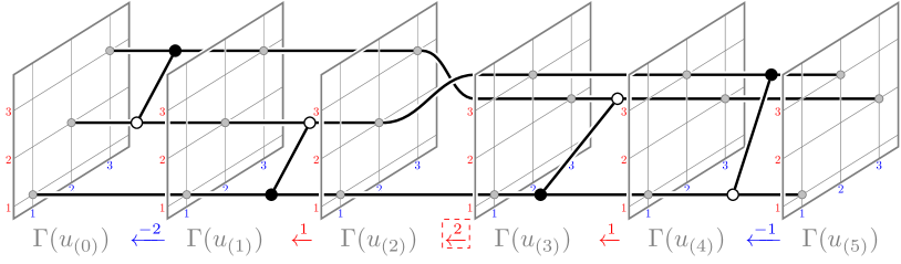
(a) 3D plabic graph $G_{u,\beta}$

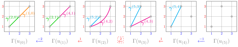
(b) monotone curves in $G_{u,\beta}$

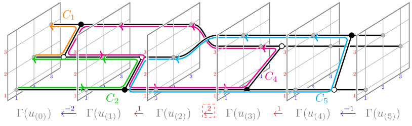
(c) relative cycles in $G_{u,\beta}$

Figure 5. A 3D plabic graph $G_{u,\beta}$ for $u=s_{2}$ and $\beta=(-2,1,2,1,-1)$; see Example 3.10.

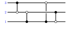
(a) $\pi_{\operatorname{red}}(G_{u,\beta})$ (b) $\pi_{\operatorname{blue}}(G_{u,\beta})$ (c) $\pi_{\operatorname{red}}(\overline{G}_{u,\beta})$

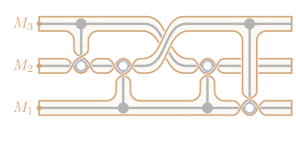
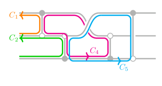
(d) $\pi_{\operatorname{red}}(\mathbf{S}_{u,\beta})$ (e) $\pi_{\operatorname{red}}(C_{c})$, $c\in J_{u,\beta}$

Figure 6. Projections of objects associated to 3D plabic graphs (cf. Figures 5 and 3.10).

3.2. 3D plabic graphs

We view permutations $z\in S_{n}$ as bijections $[n]\to[n]$, with multiplication given by composition. Thus, if $z=xy$ then we have $z(i)=x(y(i))$ for $i\in[n]$. The permutation diagram $\Gamma(z)\subset{\mathbb{Z}}^{2}$ of $z\in S_{n}$ is the set of dots $(i,z(i))$ for $i\in[n]$. We use Cartesian coordinates for permutation diagrams. Thus, the dot $(i,j)$ is located in column $i$ and row $j$, with the dot $(1,1)$ located in the bottom-left corner. We let $\preceq$ be the partial order on ${\mathbb{Z}}^{2}\subset{\mathbb{R}}^{2}$ given by $(x,y)\preceq(x^{\prime},y^{\prime})$ whenever $x\leq x^{\prime}$ and $y\leq y^{\prime}$.

We consider ${\mathbb{Z}}^{3}$ with coordinates $(i,j,t)$, where the third coordinate $t$ is referred to as the time. For each $c=0,1,\dots,m$, place the permutation diagram $\Gamma(u_{(c)})$ in the $t=c$ plane.

We now define the 3D plabic graph $G_{u,\beta}$; see Example 3.10 and Figure 5(a). We first give an informal description; see below for an explicit description in coordinates in ${\mathbb{Z}}^{3}$.

Definition 3.4.

Start by drawing $n$ strands in ${\mathbb{R}}^{3}\supset{\mathbb{Z}}^{3}$ whose time coordinate is monotone increasing, so that for $c=0,1,\dots,m$, each of the $n$ dots of $\Gamma(u_{(c)})$ belongs to exactly one strand. For each $c\in[m]$, the permutation diagrams $\Gamma(u_{(c-1)})$ and $\Gamma(u_{(c)})$ either are identical or differ by a row (if $i_{c}>0$) or by a column (if $i_{c}<0$) transposition. The strands of $G_{u,\beta}$ connect each dot of $\Gamma(u_{(c-1)})$ to the corresponding dot of $\Gamma(u_{(c)})$. In addition, for each solid crossing $c\in J_{u,\beta}$, we add a bridge edge $b_{c}$ at time $t=c-\frac{1}{2}$ between the two strands $S_{1}\prec S_{2}$ participating in the solid crossing, where the partial order $\preceq$ is extended from the dots of $\Gamma(u_{(c-1)})=\Gamma(u_{(c)})$ to the strands passing through them. If $i_{c}>0$ (resp., $i_{c}<0$), the strands $S_{1},S_{2}$ are located in adjacent rows (resp., columns), and the bridge $b_{c}$ is black at $S_{1}$ and white at $S_{2}$ (resp., white at $S_{1}$ and black at $S_{2}$). The vertex of $b_{c}$ on $S_{1}$ (resp., on $S_{2}$) is called the start (resp., the end) of $b_{c}$.

For $0<c<m$, we do not view the dots in $\Gamma(u_{(c)})$ as vertices of $G_{u,\beta}$. The dots in $\Gamma(u_{(0)})$ are viewed as degree $1$ marked boundary vertices of $G_{u,\beta}$. The dots in $\Gamma(u_{(m)})$ are viewed as unmarked degree $1$ vertices of $G_{u,\beta}$. We let $\overline{G}_{u,\beta}$ be obtained from $G_{u,\beta}$ by deleting these $n$ vertices and the $n$ edges incident to them; see Figure 6(c).

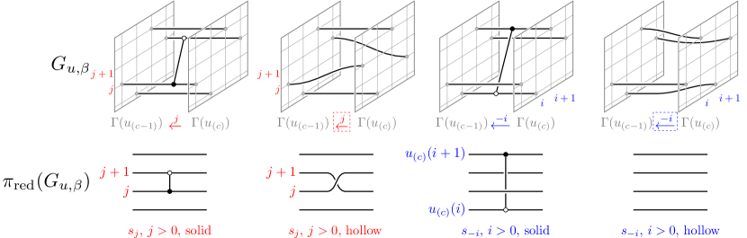
Figure 7. Applying the red projection to a 3D plabic graph.

It is convenient to project 3D plabic graphs to the plane. There are two natural choices for such projections. The red projection of $G_{u,\beta}$ is its image under the map $\pi_{\operatorname{red}}:{\mathbb{R}}^{3}\to{\mathbb{R}}^{2}$, $(i,j,t)\mapsto(t,j)$. Similarly, the blue projection of $G_{u,\beta}$ is obtained by applying the map $\pi_{\operatorname{blue}}:{\mathbb{R}}^{3}\to{\mathbb{R}}^{2}$, $(i,j,t)\mapsto(t,i)$. We will mostly work with the red projection $\pi_{\operatorname{red}}(G_{u,\beta})$; see Figures 6 and 7. We sometimes mention the faces of $\pi_{\operatorname{red}}(G_{u,\beta})$ and $\pi_{\operatorname{blue}}(G_{u,\beta})$; by this we mean connected components of the complement.

We now give a formal description of $G_{u,\beta}$. Suppose first that $c\in J_{u,\beta}$ is a solid crossing. Then $u_{(c-1)}=u_{(c)}$, and we connect each dot $(i,j,c-1)$ in $\Gamma(u_{(c-1)})$ to the corresponding dot $(i,j,c)$ of $\Gamma(u_{(c)})$, where $j=u_{(c-1)}(i)=u_{(c)}(i)$. Suppose now that $c\in[m]\setminus J_{u,\beta}$ is a hollow crossing. If $i_{c}>0$, then $\Gamma(u_{(c-1)})$ and $\Gamma(u_{(c)})$ differ by a row transposition, and we connect the dots accordingly. Specifically, letting $j:=i_{c}$, we connect:

• $(i,j,c-1)\in\Gamma(u_{(c-1)})$ to $(i,j+1,c)\in\Gamma(u_{(c)})$,

• $(i^{\prime},j+1,c-1)\in\Gamma(u_{(c-1)})$ to $(i^{\prime},j,c)\in\Gamma(u_{(c)})$, and

• $(i^{\prime\prime},j^{\prime\prime},c-1)\in\Gamma(u_{(c-1)})$ to $(i^{\prime\prime},j^{\prime\prime},c)\in\Gamma(u_{(c)})$ for $j^{\prime\prime}\neq j,j+1$.

Similarly, if $i_{c}<0$, then $\Gamma(u_{(c-1)})$ and $\Gamma(u_{(c)})$ differ by a column transposition. Letting $i:=|i_{c}|$, we connect:

• $(i,j,c-1)\in\Gamma(u_{(c-1)})$ to $(i+1,j,c)\in\Gamma(u_{(c)})$,

• $(i+1,j^{\prime},c-1)\in\Gamma(u_{(c-1)})$ to $(i,j^{\prime},c)\in\Gamma(u_{(c)})$, and

• $(i^{\prime\prime},j^{\prime\prime},c-1)\in\Gamma(u_{(c-1)})$ to $(i^{\prime\prime},j^{\prime\prime},c)\in\Gamma(u_{(c)})$ for $i^{\prime\prime}\neq i,i+1$.

We add $|J_{u,\beta}|$-many bridges to $G_{u,\beta}$. Consider a solid crossing $c\in J_{u,\beta}$. Suppose first that $i_{c}>0$ and let $j:=i_{c}$. Then $G_{u,\beta}$ contains strands connecting the dots $(i,j,c-1)$ to $(i,j,c)$ and $(i^{\prime},j+1,c-1)$ to $(i^{\prime},j+1,c)$, for some $i,i^{\prime}\in[n]$. In order for $c$ to be solid, we must have $i<i^{\prime}$. We put a black vertex on the segment connecting $(i,j,c-1)$ to $(i,j,c)$, and a white vertex on the segment connecting $(i^{\prime},j+1,c-1)$ to $(i^{\prime},j+1,c)$, and connect these two vertices by an edge, which we call a bridge and denote $b_{c}$. Suppose now that $i_{c}<0$ and let $i:=|i_{c}|$. Then $G_{u,\beta}$ contains strands connecting the dots $(i,j,c-1)$ to $(i,j,c)$ and $(i+1,j^{\prime},c-1)$ to $(i+1,j^{\prime},c)$, for some $j,j^{\prime}\in[n]$, and again we must have $j<j^{\prime}$. We put a black vertex on the segment connecting $(i,j,c-1)$ to $(i,j,c)$, and a white vertex on the segment connecting $(i+1,j^{\prime},c-1)$ to $(i+1,j^{\prime},c)$, and connect these two vertices by a bridge $b_{c}$.

3.3. Conjugate surfaces

Continuing Section 2.3, we endow the graph $G_{u,\beta}$ with the structure of a marked ribbon graph in the language of [FG06, Section 3]. A ribbon graph is a graph together with a choice, for each vertex $v$, of a cyclic orientation on the half-edges emanating from $v$. Taking the red projection of $G_{u,\beta}$, we choose the counterclockwise (resp., clockwise) orientation for each white (resp., black) vertex of $G_{u,\beta}$. The marked degree $1$ vertices of $G_{u,\beta}$ are the $n$ dots in $\Gamma(u_{(0)})$.

Remark 3.5.

From now on, we view $G_{u,\beta}$ as a ribbon graph, not as a bicolored graph. When projecting a ribbon graph $G_{u,\beta}$ to the plane, we choose the color of each vertex to be white (resp., black) if its local half-edge orientation is counterclockwise (resp., clockwise). Thus, for example, we can change the color of a given vertex $q$ by altering the drawing of $G$; see Figure 9(left). In this case, we label the resulting vertex by $\bar{q}$, emphasizing that $q$ and $\bar{q}$ represent the same vertex of $G$.

We let $\mathbf{S}_{u,\beta}=\mathbf{S}(G_{u,\beta})$ be the marked surface with boundary associated to $G_{u,\beta}$ in a standard way: we replace every edge of $G_{u,\beta}$ by a thin rectangle, every vertex of $G_{u,\beta}$ by a disk, and glue the rectangles to the boundaries of the disks according to the local orientation around each vertex. Thus, $\partial\mathbf{S}_{u,\beta}$ has several connected components, and we stress that we do not glue disks to them. The surface $\mathbf{S}_{u,\beta}$ can be drawn using the red projection of $G_{u,\beta}$ as shown in Figure 6(d). In particular, $\mathbf{S}_{u,\beta}$ is orientable, with black and white vertices in the red projection of $G_{u,\beta}$ corresponding to the different sides of $\mathbf{S}_{u,\beta}$.

We apply a similar construction to $\overline{G}_{u,\beta}$, and it is clear that the resulting surface $\mathbf{S}(\overline{G}_{u,\beta})$ is homeomorphic to $\mathbf{S}_{u,\beta}$.

Let $\mathbf{M}$ be the set of marked points on $\partial\mathbf{S}_{u,\beta}$; thus, $|\mathbf{M}|=n$. Let $\Lambda_{u,\beta}:=H_{1}(\mathbf{S}_{u,\beta},\mathbf{M})$. (All relative homology groups we consider are with integer coefficients.) The elements of $\Lambda_{u,\beta}$, called relative cycles, are represented by ${\mathbb{Z}}$-linear combinations of arcs, where an arc is either an oriented closed curve embedded into the interior of $\mathbf{S}_{u,\beta}$ or an oriented curve embedded into $\mathbf{S}_{u,\beta}$ with both endpoints marked. Let $\Lambda^{\ast}_{u,\beta}:=H_{1}(\mathbf{S}_{u,\beta}\setminus\mathbf{M},\partial\mathbf{S}_{u,\beta}\setminus\mathbf{M})$. We have an intersection form on $(\mathbf{S}_{u,\beta},\mathbf{M})$ which gives rise to a perfect pairing

(3.2) $${\langle}\cdot,\cdot{\rangle}:\Lambda_{u,\beta}\otimes\Lambda^{\ast}_{u,\beta}\to{\mathbb{Z}};$$

see e.g. [CW22, Proposition 3.48] or [Mel19, Section 6.1]. For $C\in\Lambda_{u,\beta}$, $C^{\prime}\in\Lambda^{\ast}_{u,\beta}$, the intersection number ${\langle}C,C^{\prime}{\rangle}$ is the integer obtained by counting signed intersection points between two generic relative cycles representing $C$ and $C^{\prime}$.

Remark 3.6.

An oriented cycle in $G_{u,\beta}$ can be naturally lifted to an element of $\Lambda_{u,\beta}$ as well as to an element of $\Lambda^{\ast}_{u,\beta}$. On the other hand, an oriented path with both endpoints marked can only be naturally lifted to an element of $\Lambda_{u,\beta}$.

3.4. Relative cycles

Fix a solid crossing $c\in J_{u,\beta}$. Our goal is to associate to it a relative cycle $C_{c}\in\Lambda_{u,\beta}$. As in Section 2.2, we will obtain $C_{c}$ as the boundary of a certain $2$-dimensional disk $D_{c}$ inside ${\mathbb{R}}^{3}$.

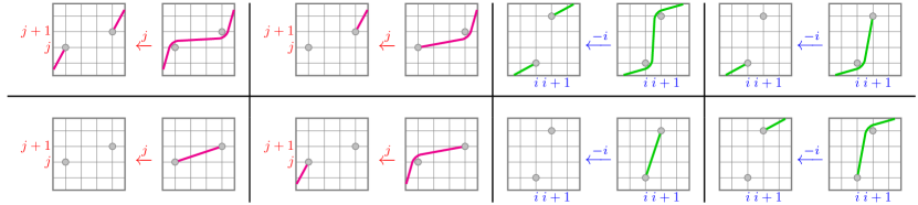
Figure 8. Propagation rules for monotone curves; see Section 3.4. In any case not depicted here, the monotone curve is unchanged by the action of a solid crossing.

A monotone curve inside a permutation diagram $\Gamma(z)\subset{\mathbb{R}}^{2}$ is a curve $\gamma:[0,1]\to{\mathbb{R}}^{2}$ whose endpoints are dots in $\Gamma(z)$, with no other dots of $\Gamma(z)$ on $\gamma$, and such that both coordinates of $\gamma$ are strictly monotone increasing. Recall that we write $(x,y)\preceq(x^{\prime},y^{\prime})$ if $x\leq x^{\prime}$ and $y\leq y^{\prime}$. Write $(x,y)\prec(x^{\prime},y^{\prime})$ if $(x,y)\preceq(x^{\prime},y^{\prime})$ and $(x,y)\neq(x^{\prime},y^{\prime})$. Thus, $\gamma(0)\prec\gamma(1)$. A monotone multicurve is a collection $\bm{\gamma}=(\gamma_{1},\gamma_{2},\dots,\gamma_{k})$ of monotone curves inside $\Gamma(z)$ such that

$$\gamma_{1}(0)\prec\gamma_{1}(1)\prec\gamma_{2}(0)\prec\gamma_{2}(1)\prec\cdots\prec\gamma_{k}(0)\prec\gamma_{k}(1).$$

The intersection of the disk $D_{c}$ with each plane $t=r$, $0\leq r\leq c-1$, will be a monotone multicurve inside $\Gamma(u_{(r)})$ denoted $\bm{\gamma}^{(c,r)}$. For $r=c-1$, $\bm{\gamma}^{(c,c-1)}$ consists of a single monotone curve connecting the two dots on the strands which are connected by $b_{c}$. We then compute $\bm{\gamma}^{(c,r)}$ iteratively for $r=c-2,\dots,1,0$, using the following propagation rules. When passing from $\bm{\gamma}^{(c,r)}$ to $\bm{\gamma}^{(c,r-1)}$ for a solid crossing $r$, each monotone curve $\gamma$ in $\bm{\gamma}^{(c,r)}$ either is preserved or gets cut. The cutting moves are shown in Figure 8, and all other curves not shown in Figure 8 are preserved. When the crossing $r$ is hollow, each monotone curve $\gamma$ changes “smoothly” so that a dot $\mathfrak{d}$ of $\Gamma(u_{(r)})$ is above (resp., below) $\gamma$ if and only if the dot $\mathfrak{d}^{\prime}$ of $\Gamma(u_{(r-1)})$ that is on the same strand as $\mathfrak{d}$ is above (resp., below) the image of $\gamma$ in $\Gamma(u_{(r-1)})$; see e.g. Figure 5(b).

To give a coordinate description in the case of a solid crossing, let $r\in J_{u,\beta}$ be such that $i_{r}>0$ and let $j:=i_{r}$. Let $\mathfrak{d}:=(i,j)$ and $\mathfrak{d}^{\prime}:=(i^{\prime},j+1)$ be the dots in $\Gamma(u_{(r)})=\Gamma(u_{(r-1)})$, for some $i,i^{\prime}\in[n]$. Then the curve $\gamma$ gets cut if and only if it passes weakly above $\mathfrak{d}$ and weakly below $\mathfrak{d}^{\prime}$. Assume now that $i_{r}<0$ and let $i:=|i_{r}|$. Let $\mathfrak{d}:=(i,j)$ and $\mathfrak{d}^{\prime}:=(i+1,j^{\prime})$ be the dots in $\Gamma(u_{(r)})=\Gamma(u_{(r-1)})$, for some $j,j^{\prime}\in[n]$. Then $\gamma$ gets cut if and only if it passes weakly to the right of $\mathfrak{d}$ and weakly to the left of $\mathfrak{d}^{\prime}$. In both cases, the cutting move consists of removing the part of $\gamma$ passing between $\mathfrak{d}$ and $\mathfrak{d}^{\prime}$. (In particular, if neither $\mathfrak{d}$ nor $\mathfrak{d}^{\prime}$ was an endpoint of $\gamma$ then we split $\gamma$ into two monotone curves $\gamma^{\prime},\gamma^{\prime\prime}$ satisfying $\gamma^{\prime}(1)=\mathfrak{d}$ and $\gamma^{\prime\prime}(0)=\mathfrak{d}^{\prime}$. On the other hand, if both $\mathfrak{d}$ and $\mathfrak{d}^{\prime}$ were endpoints of $\gamma$ then the whole of $\gamma$ disappears.)

Definition 3.7.

If $\bm{\gamma}^{(c,0)}$ is empty, then we declare $c$ to be mutable, otherwise, we declare $c$ to be frozen. We let $J_{u,\beta}^{\operatorname{fro}}$ and $J_{u,\beta}^{\operatorname{mut}}$ denote the sets of frozen and mutable indices, respectively.

Thus, we have a decomposition $J_{u,\beta}=J_{u,\beta}^{\operatorname{fro}}\sqcup J_{u,\beta}^{\operatorname{mut}}$.

If $c$ is mutable, we obtain a disk $D_{c}$ inside ${\mathbb{R}}^{3}$ whose boundary $\partial D_{c}$ is a cycle $C_{c}$ in $G_{u,\beta}$ that does not pass through any marked points. If $c$ is frozen, we treat $\bm{\gamma}^{(c,0)}$ as part of the boundary of the disk $D_{c}$, and denote the rest of $\partial D_{c}$ by $C_{c}:=\partial D_{c}\setminus\bm{\gamma}^{(c,0)}$. In both cases, $\partial D_{c}$ passes through the bridge $b_{c}$, and we orient $\partial D_{c}$ so that it is directed from the start to the end of $b_{c}$; cf. Definition 3.4. This induces an orientation on each arc in $C_{c}$, and therefore we obtain a relative cycle $C_{c}\in\Lambda_{u,\beta}$. See Figures 5(c) and 6(e).

Figure 9. Left: switching the color of a vertex. Middle: contraction-uncontraction move (M1) and square move (M2). Right: sign convention for the intersection form of $\mathbf{S}_{u,\beta}$.

3.5. The quiver

Our goal is to associate an ice quiver $\widetilde{Q}_{u,\beta}$ to the pair $(u,\beta)$.

The vertex set of $\widetilde{Q}_{u,\beta}$ is $\widetilde{V}:=J_{u,\beta}$, with frozen vertices $V^{\operatorname{fro}}:=J_{u,\beta}^{\operatorname{fro}}$ and mutable vertices $V^{\operatorname{mut}}:=J_{u,\beta}^{\operatorname{mut}}$ (cf. Definition 3.7). Let $c\in\widetilde{V}$ and $d\in V^{\operatorname{mut}}$, and consider the corresponding relative cycles $C_{c},C_{d}$. By Remark 3.6, we may view $C_{d}$ as an element of $\Lambda^{\ast}_{u,\beta}$. The cluster exchange matrix $\widetilde{B}(\widetilde{Q}_{u,\beta})=(\tilde{b}_{c,d})_{c\in\widetilde{V},d\in V^{\operatorname{mut}}}$ of $\widetilde{Q}_{u,\beta}$ is given by

(3.3) $$\tilde{b}_{c,d}=\#\{\text{arrows $c\to d$ in $\widetilde{Q}$}\}-\#\{\text{arrows $d\to c$ in $\widetilde{Q}$}\}:={\langle}C_{c},C_{d}{\rangle}.$$

In other words, the (signed) number of arrows from $c$ to $d$ in $\widetilde{Q}_{u,\beta}$ is given by the intersection number ${\langle}C_{c},C_{d}{\rangle}$. We give an explicit algorithm for computing intersection numbers.

Algorithm 3.8.

The intersection form ${\langle}C,C^{\prime}{\rangle}$ of the surface $\mathbf{S}_{u,\beta}=\mathbf{S}(G_{u,\beta})$ may be computed as follows. See Figure 10 and the top row of Figure 13(right) for examples.

• Viewing $C,C^{\prime}$ as subgraphs of $G_{u,\beta}$, decompose $C\cap C^{\prime}$ into a union of disjoint paths.

• For each of these paths $P$, we will have a contribution ${\langle}C,C^{\prime}{\rangle}|_{P}\in\{-1,0,1\}$; the intersection number ${\langle}C,C^{\prime}{\rangle}$ will be the sum of ${\langle}C,C^{\prime}{\rangle}|_{P}$ over the components $P$ of $C\cap C^{\prime}$.

• Let $P=(p_{0},p_{1},\ldots,p_{r})$ be one of the paths. The contribution ${\langle}C,C^{\prime}{\rangle}|_{P}$ will depend only on which neighbors of $p_{0}$ and $p_{r}$ are visited by $C$ and $C^{\prime}$, and in which order.

• Draw $P$ in the plane with all vertices black (cf. Remark 3.5) and perturb $C,C^{\prime}$ slightly so that they have either zero or one intersection point.

• If $C,C^{\prime}$ have zero intersection points, we have ${\langle}C,C^{\prime}{\rangle}|_{P}=0$.

• If $C,C^{\prime}$ have one intersection point $p$, we have ${\langle}C,C^{\prime}{\rangle}|_{P}=+1$ if the tangent vectors of $(C,C^{\prime})$ at $p$ form a positively oriented basis of the plane and ${\langle}C,C^{\prime}{\rangle}|_{P}=-1$ otherwise; see Figure 9(right).

Remark 3.9.

As we pointed out in Section 3.3, the surface $\mathbf{S}_{u,\beta}$ is orientable. It follows that we have ${\langle}C_{d},C_{d}{\rangle}=0$ for all mutable $d\in J_{u,\beta}$.

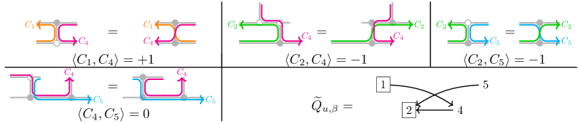
Figure 10. Computing the quiver $\widetilde{Q}_{u,\beta}$ corresponding to Figures 5, 6 and 3.10; see Algorithm 3.8.

Example 3.10.

Let $u:=s_{2}\in S_{3}$ and $\beta:=(-2,1,2,1,-1)$. Thus, $J_{u,\beta}=\{1,2,4,5\}$. The graph $G_{u,\beta}$ is given in Figure 5(a), and its red and blue projections are shown in Figure 6(a,b), respectively. The monotone (multi)curves are computed in Figure 5(b) using the propagation rules from Figure 8. The relative cycles $(C_{c})_{c\in J_{u,\beta}}$ are shown in Figures 5(c) and 6(e), and the surface $\mathbf{S}_{u,\beta}$ is shown in Figure 6(d). In Figure 10, we use this data to compute the intersection numbers ${\langle}C_{c},C_{d}{\rangle}$ and the quiver $\widetilde{Q}_{u,\beta}$ via Algorithm 3.8. The frozen vertices of $\widetilde{Q}_{u,\beta}$ are boxed in Figure 10.

Remark 3.11.

The simplified propagation rules shown in Figure 3 are obtained from the rules in Figure 8 by applying the red projection. It is therefore important to distinguish between over/under-crossings when applying the rules in Figure 3 to the red projection of a 3D plabic graph in Figure 3. However, the ribbon graph $G_{u,\beta}$ and the associated surface $\mathbf{S}_{u,\beta}$ are most naturally considered as abstract objects without a fixed choice of an embedding in ${\mathbb{R}}^{3}$. Thus, in the rest of our figures, e.g., when drawing the boundary of $\mathbf{S}_{u,\beta}$ in Figure 6(d) or the graphs in Figures 23–25, the over/under-crossings are irrelevant, and are chosen arbitrarily.

Definition 3.12.

Given an ice quiver $\widetilde{Q}$ and a mutable vertex $d\in V^{\operatorname{mut}}$, one can mutate $\widetilde{Q}$ in direction $d$ to obtain another quiver $\widetilde{Q}^{\prime}=\mu_{d}(\widetilde{Q})$, the mutation of $\widetilde{Q}$ at $d$. Mutation preserves the sets of mutable and frozen vertices, and changes the arrows as follows:

• for each directed path $c\to d\to e$ in $\widetilde{Q}$ of length $2$, add an arrow $c\to e$ to $\widetilde{Q}^{\prime}$;

• reverse all arrows in $\widetilde{Q}$ incident to $d$;

• remove all directed $2$-cycles in the resulting directed graph, one at a time.

This operation may create arrows between pairs of frozen vertices; such pairs are omitted.

Recall that the quiver $\widetilde{Q}_{u,\beta}$ is obtained from the collection $(C_{c})_{c\in J_{u,\beta}}$ of relative cycles in $\Lambda_{u,\beta}$ via (3.3). Following [GK13, Section 4.1.2] and [FG09, Section 1.2], we explain how for each $d\in J_{u,\beta}^{\operatorname{mut}}$, the quiver $\mu_{d}(\widetilde{Q}_{u,\beta})$ is obtained in the same way via (3.3) from another collection $(\mu_{d}(C_{c}))_{c\in J_{u,\beta}}$ of relative cycles in $\Lambda_{u,\beta}$. Namely, we set

(3.4) $$\mu_{d}(C_{c}):=\begin{cases}C_{c}+\max\left({\langle}C_{c},C_{d}{\rangle},0\right)C_{d},&\text{if $c\neq d$,}\\ -C_{d},&\text{ if $c=d$.}\end{cases}$$

Since $d$ is mutable, we see that for each mutable $c$, the relative cycle $\mu_{d}(C_{c})$ is still naturally an element of both $\Lambda_{u,\beta}$ and $\Lambda^{\ast}_{u,\beta}$.

Lemma 3.13 ([FG09, Lemma 1.7]).

The exchange matrix of $\mu_{d}(\widetilde{Q}_{u,\beta})$ is given via (3.3) by the intersection numbers of the relative cycles $(\mu_{d}(C_{c}))_{c\in J_{u,\beta}}$.

Remark 3.14.

We will show in Section 5.3 that $(C_{c})_{c\in J_{u,\beta}}$ is a ${\mathbb{Z}}$-basis of $\Lambda_{u,\beta}$. It follows that $(\mu_{d}(C_{c}))_{c\in J_{u,\beta}}$ is a ${\mathbb{Z}}$-basis of $\Lambda_{u,\beta}$ as well.

3.6. Distinguished subexpressions

The goal of this section is to explain how the propagation rules for monotone curves from Section 3.4 reflect the combinatorics of almost positive subexpressions. These results will be used in Section 7 for comparison to geometry.

Let $\beta\in(\pm I)^{m}$ be a double braid word and $u\leq\beta$. A $u$-subexpression ${\mathbf{u}}$ of $\beta$ is called distinguished if $u_{(c)}\leq s_{i_{c}}^{-}u_{(c-1)}s_{i_{c}}^{+}$ for each $c\in[m]$. This notion originated in the study of the geometry of open Richardson varieties [Deo85, MR04, WY07].

Definition 3.15.

Let $d\in J_{u,\beta}$. Let $v_{(m)}^{{\langle}d{\rangle}}:=u$, and for $c=m,m-1,\dots,1$, define

$$v_{(c-1)}^{{\langle}d{\rangle}}:=\begin{cases}s_{i_{d}}^{-}\ast v_{(d)}^{{\langle}d{\rangle}}\ast s_{i_{d}}^{+},&\text{if $c=d$,}\\ s_{i_{c}}^{-}\vartriangleright v_{(c)}^{{\langle}d{\rangle}}\vartriangleleft s_{i_{c}}^{+},&\text{otherwise}.\end{cases}$$

We call the sequence $(v^{{\langle}d{\rangle}}_{(0)},\dots v^{{\langle}d{\rangle}}_{(m)})$ the $(u,d)$-almost positive sequence ($(u,d)$-APS).

In other words, the $u$-PDS is obtained by starting with $u$ and taking successive Demazure quotients according to the letters of $\beta$. The $(u,d)$-APS is obtained by taking Demazure quotients up to crossing $d$; then making a “mistake” at crossing $d$ and taking Demazure product rather than Demazure quotient; then continuing to take Demazure quotients.

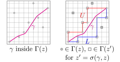
Figure 11. Recovering the almost positive subexpression from the corresponding monotone curve.

Consider a monotone curve $\gamma$ inside a permutation diagram $\Gamma(z)$ for $z\in S_{n}$. Take the smallest skew shape ${\lambda}/\mu$ containing $\gamma$ whose inner corners are at the dots of $\Gamma(z)$, and let $L$ and $U$ be its lower and upper boundaries, respectively; see Figure 11. Let $\mathfrak{D}_{\gamma}$ be the set of dots of $\Gamma(z)$ contained in $U\cup L$. Let $\mathfrak{D}^{\prime}_{\gamma}$ be the set of outer corners of ${\lambda}/\mu$, i.e., the set of lattice points where $L$ turns left or $U$ turns right. We define $z^{\prime}:=\sigma(\gamma,z)\in S_{n}$ to be the permutation such that $\Gamma(z^{\prime})$ is obtained from $\Gamma(z)$ by replacing the dots in $\mathfrak{D}_{\gamma}$ with the dots in $\mathfrak{D}^{\prime}_{\gamma}$. Given a monotone multicurve $\bm{\gamma}=(\gamma_{1},\gamma_{2},\dots,\gamma_{k})$, we let $\sigma(\bm{\gamma},z):=\sigma(\gamma_{1},\sigma(\gamma_{2},\dots,\sigma(\gamma_{k},z)\dots)).$ The following result explains the relation between monotone curves and almost positive subexpressions.

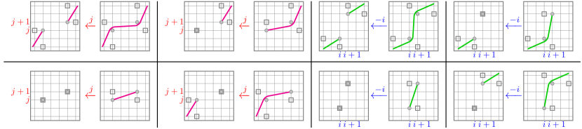
Figure 12. Propagation rules (Figure 8) shown together with the corresponding almost positive subexpressions.

Proposition 3.16.

Let $d\in J_{u,\beta}$. Then for all $c\leq d-1$, we have

(3.5) $$v^{{\langle}d{\rangle}}_{(c)}=\sigma(\bm{\gamma}^{d,c},u_{(c)}).$$

Démonstration.

For $c=d-1$, the permutations $v^{{\langle}d{\rangle}}_{(c)}$ and $u_{(c)}$ differ by a single transposition which corresponds to creating the monotone curve $\bm{\gamma}^{(d,d-1)}$. For $c=d-2,\dots,0$, we check (3.5) by induction, since the propagation rules of Figure 8 turn out to exactly reflect the application of Demazure quotient to pairs $(u_{(c)},v^{{\langle}d{\rangle}}_{(c)})$; see Figure 12. ∎

Corollary 3.17.

A solid index $d\in J_{u,\beta}$ is mutable if and only if $v^{{\langle}d{\rangle}}_{(0)}={\operatorname{id}}$.

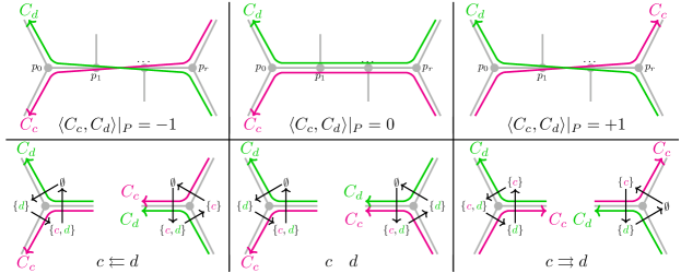
Figure 13. The half-arrow description of $\widetilde{Q}_{u,\beta}$; see Section 3.7.

3.7. Half-arrow description of $\widetilde{Q}_{u,\beta}$

We give an alternative description of $\widetilde{Q}_{u,\beta}$ that will be useful in Proposition 7.17. For each red crossing $c\in J_{u,\beta}$, $i_{c}>0$, consider the four faces $A,B,C,D$ around the red projection of the bridge $b_{c}$ as shown in Figure 13(left). To each face $X\in\{A,B,C,D\}$ we associate a collection $\nabla^{+}(X)$ of indices $d\in J_{u,\beta}$ such that $X$ is inside the red projection of the disk $D_{d}$; cf. (2.1). Then for each pair $(X,Y)=(A,B),(B,D),(D,A),(C,B),(B,D),(D,C)$ (note that $(B,D)$ is listed twice), we draw a half-arrow from each element of $\nabla^{+}(X)$ to each element of $\nabla^{+}(Y)$. Similarly, for each blue crossing $c\in J_{u,\beta}$, $i_{c}<0$, we consider the four faces $A,B,C,D$ in the blue projection, and then for each $(X,Y)=(A,B),(B,D),(D,A),(C,B),(B,D),(D,C)$, we draw a half-arrow from each element of $\nabla^{-}(Y)$ to each element of $\nabla^{-}(X)$. Here, $\nabla^{-}(X)$ is the set of indices $d\in J_{u,\beta}$ such that $X$ is inside the blue projection of $D_{b}$. We obtain a collection of half-arrows between the elements of $J_{u,\beta}$.

Proposition 3.18.

For $c,d\in J_{u,\beta}$, the difference between the number of half-arrows $c\to d$ and the number of half-arrows $d\to c$ equals $2{\langle}C_{c},C_{d}{\rangle}$.

In other words, by (3.3), the quiver $\widetilde{Q}_{u,\beta}$ is obtained by just summing up the signed half-arrow contributions and dividing the result by $2$.

Démonstration.

The above half-arrow description can be replaced by the following local description. Consider a vertex $p$ of $G_{u,\beta}$, and draw the neighborhood of $\mathbf{S}_{u,\beta}$ around $p$ so that $p$ is black. Label the faces around $p$ by $A,B,C$ in counterclockwise order. For $X\in\{A,B,C\}$, let $\nabla_{p}(X)$ denote the set of indices $c\in J_{u,\beta}$ such that $C_{c}$ passes through $p$ with $X$ to the left of $C_{c}$. Then for each $(X,Y)=(A,B),(B,C),(C,A)$, draw a half-arrow from each element of $\nabla_{p}(X)$ to each element of $\nabla_{p}(Y)$.

Consider two relative cycles $C_{c},C_{d}$, for $c,d\in J_{u,\beta}$. Recall from Algorithm 3.8 that the intersection number ${\langle}C_{c},C_{d}{\rangle}$ may be computed as a sum of local contributions ${\langle}C_{c},C_{d}{\rangle}|_{P}$ from maximal by inclusion paths in $C_{c}\cap C_{d}$. Such contributions are shown in the top row of Figure 13(right). On the other hand, as shown in the bottom row of Figure 13(right), the (signed) contribution to the number of half-arrows $c\to d$ is $\pm 1$ for $p_{0}$ and $p_{r}$ (and zero for each of $p_{1},\dots,p_{r-1}$) so that the combined half-arrow contribution from $p_{0}$ and $p_{r}$ is exactly $2{\langle}C_{c},C_{d}{\rangle}|_{P}$. Summing over all such paths $P$, the result follows. ∎

3.8. Postnikov’s plabic graphs

We explain how our 3D plabic graphs generalize the plabic graphs of [Pos06]. A permutation $w\in S_{n}$ is called $k$-Grassmannian if $w(1)<\dots<w(n-k)$ and $w(n-k+1)<\dots<w(n)$. We denote by $S_{n}^{(k)}$ the set of $k$-Grassmannian permutations. Thus, any reduced word for $w\in S_{n}^{(k)}$ ends with $s_{n-k}$, and all reduced words for $w$ are related by commutation moves. It is well known that $k$-Grassmannian permutations are in bijection with Young diagrams that fit inside a $k\times(n-k)$ rectangle. We draw Young diagrams in English notation. A Le-diagram is a way of placing a dot in some of the boxes of ${\lambda}$ so that whenever a box of ${\lambda}$ has a dot above it in the same column and to the left of it in the same row, it must also contain a dot. For each dot, we draw horizontal and vertical line segments connecting it to the southeastern boundary of ${\lambda}$. An example of a Le-diagram $\Gamma$ is shown in Figure 14(left). One can convert a Le-diagram $\Gamma$ into a plabic graph $G(\Gamma)$ using the local rule . The graph $G(\Gamma)$ is drawn in a disk which we identify with the Young diagram ${\lambda}$. Thus, $G(\Gamma)$ has $n$ boundary vertices on the southeastern boundary of ${\lambda}$, and it has a unique northwestern boundary face which we denote $F_{0}$. Rotating $\Gamma$ by $135^{\circ}$ clockwise, replacing all empty boxes with crossings, and all dots with black-white bridges, we obtain a graph $G_{u,{\mathbf{w}}}$, where ${\mathbf{w}}$ is a reduced word for $w$ and $u\leq w$ in the Bruhat order on $S_{n}$; see Figure 14.

Figure 14. Left: converting a Le-diagram $\Gamma$ into a plabic graph $G(\Gamma)$. Right: the graphs $G_{u,{\mathbf{w}}}$ and $\overline{G}_{u,{\mathbf{w}}}$ for $(u,w)$ corresponding to $\Gamma$.

Proposition 3.19.

Let $\Gamma$ be a Le-diagram and let $u\leq w$ be the corresponding pair of permutations. Then we have

$$G(\Gamma)=\overline{G}_{u,{\mathbf{w}}}.$$

Moreover, each relative cycle $C_{c}$ of $\overline{G}_{u,{\mathbf{w}}}$ traverses the boundary of a face of $G(\Gamma)$ in the counterclockwise direction, and this gives a bijection between the relative cycles $(C_{c})_{c\in J_{u,{\mathbf{w}}}}$ and all faces of $G(\Gamma)$ except $F_{0}$.

Démonstration.

It follows from the definition of a Le-diagram that once a strand in $G_{u,{\mathbf{w}}}$ participates in a hollow crossing, it never participates in a solid crossing to the right of that hollow crossing. In particular, all hollow crossings disappear when we pass from $G_{u,{\mathbf{w}}}$ to $\overline{G}_{u,{\mathbf{w}}}$, and thus it follows that $G(\Gamma)=\overline{G}_{u,{\mathbf{w}}}$; see also [Kar16, Figure 5] and [GL19, Figure 7]. An example is given in Figure 14(right).

To compute the relative cycles in $G_{u,{\mathbf{w}}}$, we may use the propagation rules in Figure 3. From here, the statement that the relative cycles correspond to the faces of $G(\Gamma)$ follows immediately. ∎

4. Invariance under moves

In this section, we show that the mutation class of the quiver $\widetilde{Q}_{u,\beta}$ defined above is invariant under applying double braid moves to $\beta$.

4.1. Moves for 3D plabic graphs

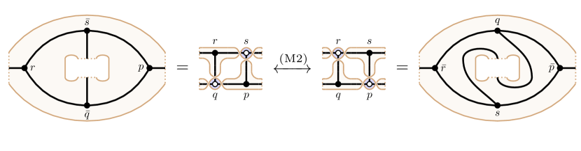
Figure 15. Applying a square move (M2) to $G_{u,\beta}$ preserves the surface $\mathbf{S}_{u,\beta}$ but changes the embedding of $G_{u,\beta}$ in $\mathbf{S}_{u,\beta}$. See also [GK13, Figure 20].

Just as in Postnikov’s theory [Pos06], our two main moves for 3D plabic graphs are the contraction-uncontraction move (M1) and the square move (M2), shown in Figure 9(middle). The move (M1) can be performed on any edge $e=\{p,q\}$ of a 3D plabic graph $G$. Specifically, we draw $G$ in the plane so that $p$ and $q$ are of the same color, and then we apply the usual contraction-uncontraction move, producing two other vertices of the same color as $p$ and $q$. The move (M2) can be performed on any $4$-cycle $(p,q,r,s)$ in $G$, as shown in Figure 15. The moves (M1)–(M2) preserve the conjugate surface $\mathbf{S}=\mathbf{S}(G)$ but change the embedding of $G$ inside of $\mathbf{S}$. In particular, it will be important later that as one applies the various double braid moves to the double braid word $\beta$, the surface $\mathbf{S}_{u,\beta}$ stays unchanged throughout the process.

Remark 4.1.

Surprisingly, the square move (M2) can be obtained by performing two contraction-uncontraction moves (M1) on $G$; see Figure 16. We still distinguish (M2) as a separate transformation, for the following reason. We have associated three kinds of objects to a pair $(u,\beta)$: a 3D plabic graph $G_{u,\beta}$, a marked surface $\mathbf{S}_{u,\beta}$, and a collection $(C_{c})_{c\in J_{u,\beta}}$ of relative cycles in $\mathbf{S}_{u,\beta}$. While $G_{u,\beta}$ determines $\mathbf{S}_{u,\beta}$, neither $G_{u,\beta}$ nor $\mathbf{S}_{u,\beta}$ determines $(C_{c})_{c\in J_{u,\beta}}$. Thus, if one applies moves (M1)–(M2) to $G_{u,\beta}$, one has to specify additional rules for how the tuple $(C_{c})_{c\in J_{u,\beta}}$ changes. These rules are given in Theorem 4.3 below: the tuple $(C_{c})_{c\in J_{u,\beta}}$ changes according to (3.4) when we apply mutation braid moves corresponding to (M2), and is preserved when we apply non-mutation braid moves corresponding to other sequences of moves (M1).

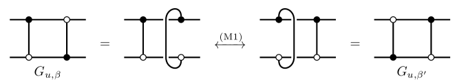
Figure 16. Representing the square move (M2) as a composition of two contraction-uncontraction moves (M1).

4.2. Moves for double braid words

Two double braid words are (double braid) equivalent if they are related by a sequence of the following double braid moves:

1. $ij\leftrightarrow ji$  if $i,j\in\pm I$ have different signs;

2. $ij\leftrightarrow ji$  if $i,j\in\pm I$ have the same sign and $|i-j|>1$;

3. $iji\leftrightarrow jij$  if $i,j\in\pm I$ have the same sign and $|i-j|=1$.

Definition 4.2.

We say that a double braid move is fully solid if all of the indices involved are solid. Suppose that $i_{d-1}=-j$ and $i_{d}=i$ for some $i,j\in I$ and $2\leq d\leq m$. Then we say that the move (B1) swapping these two indices is special if $u_{(d-1)}s_{i}=s_{j}u_{(d-1)}$, and solid-special if it is special and fully solid. Motivated by the following theorem, we call  (B1) (solid-special) and (B3) (fully solid) mutation moves. All other braid moves are non-mutation moves.

Theorem 4.3.

The mutation type of $\widetilde{Q}_{u,\beta}$ is invariant under double braid moves (B1)–(B3) on $\beta$. More precisely:

1. Under mutation moves, the quiver $\widetilde{Q}_{u,\beta}$ changes by a mutation. The relative cycles $(C_{c})_{c\in J_{u,\beta}}$ change according to (3.4). The graph $G_{u,\beta}$ changes by a square move (M2).

2. Under non-mutation moves, the quiver $\widetilde{Q}_{u,\beta}$ and the relative cycles $(C_{c})_{c\in J_{u,\beta}}$ are unchanged, up to relabeling. The graph $G_{u,\beta}$ changes by a sequence of contraction-uncontraction moves (M1).

In both cases, the surface $\mathbf{S}_{u,\beta}$ is unchanged.

We prove Theorem 4.3 in the next two subsections. Throughout, we let $\beta$ and $\beta^{\prime}$ be two braids related by one of the moves in Theorem 4.3. We denote the 3D plabic graphs by $G_{u,\beta}$ and $G_{u,\beta^{\prime}}$, the surfaces by $\mathbf{S}_{u,\beta}$ and $\mathbf{S}_{u,\beta^{\prime}}$, and the relative cycles by $(C_{c})_{c\in J_{u,\beta}}$ and $(C^{\prime}_{c})_{c\in J_{u,\beta^{\prime}}}$, respectively.

Figure 17. Applying braid moves from part (1) of Theorem 4.3 results in applying a square move to $G_{u,\beta}$.

4.3. Mutation moves

We prove part (1) of Theorem 4.3. Assume that we are applying a mutation move involving either the indices $i_{d-1},i_{d}$ or $i_{d-2},i_{d-1},i_{d}$ for some $d\in J_{u,\beta}$. By Lemma 3.13, it suffices to show that the relative cycles change according to (3.4), i.e., that $C^{\prime}_{c}=\mu_{d}(C_{c})$ for all $c\in J_{u,\beta}$.

4.3.1. Applying (B1) (solid-special)

We would like to swap two solid crossings $i_{d-1}=-i$ and $i_{d}=j$ (with $i,j\in I$) such that $u_{(d-1)}s_{i}=s_{j}u_{(d-1)}$. Since $d-1,d$ are both solid, we have $u_{(d-2)}=u_{(d-1)}=u_{(d)}$. In addition, using $u_{(d)}s_{i}=s_{j}u_{(d)}$, we find that $u_{(d)}(i)=j$ and $u_{(d)}(i+1)=j+1$. The graph $G_{u,\beta}$ therefore contains a $4$-cycle spanned by the pair $(b_{d-1},b_{d})$ of bridges of opposite color; see Figure 17(left). It follows that the graph $G_{u,\beta^{\prime}}$ is obtained from $G_{u,\beta}$ by applying a square move (M2). In particular, we have $\mathbf{S}_{u,\beta}=\mathbf{S}_{u,\beta^{\prime}}$; see Figure 15.

We will show that $C^{\prime}_{c}=\mu_{d}(C_{c})$ by classifying all possible cases of how a relative cycle $C_{c}$ can look around the square $psrq$. This amounts to classifying the behavior of the monotone multicurves $\bm{\gamma}^{(c,d)},\bm{\gamma}^{(c,d-1)},\bm{\gamma}^{(c,d-2)}$ around the dots $\mathfrak{d}:=(i,j)$ and $\mathfrak{d}^{\prime}:=(i+1,j+1)$ of $\Gamma(u_{(d)})$. Note that, with the exception of the relative cycles $C_{d}$ and $C_{d-1}$, the monotone multicurve $\bm{\gamma}^{(c,d)}$ determines $\bm{\gamma}^{(c,d-1)}$ and $\bm{\gamma}^{(c,d-2)}$. Moreover, it suffices to consider the behavior of each monotone curve of $\bm{\gamma}^{(c,d)}$ separately; cf. Remark 4.4 below.

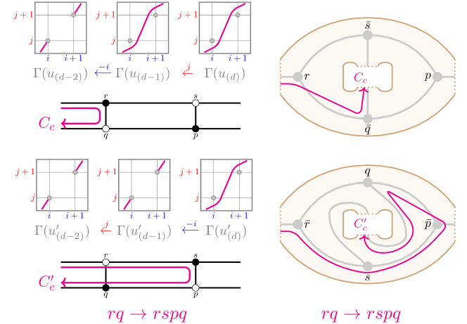
Figure 18. An example of computing the signature $rq\to rspq$ of a relative cycle $C_{c}$ under the move (B1) (solid-special).

For a relative cycle $C_{c}$ in $G_{u,\beta}$, its signature is the ordered list of vertices of the square $psrq$ that $C_{c}$ passes through. For example, let us consider a monotone curve $\gamma$ inside $\Gamma(u_{(d)})$ passing below $\mathfrak{d}$ and above $\mathfrak{d}^{\prime}$, as in Figure 18. Using the rules in Figure 8, we propagate $\gamma$ to $\Gamma(u_{(d-1)})$ and $\Gamma(u_{(d-2)})$, and find that the relevant part of $C_{c}$ passes first through $r$ and then through $q$ in $G_{u,\beta}$. Therefore, the signature of this relative cycle is $rq$. Repeating the same procedure for the graph $G_{u,\beta^{\prime}}$, we find that the signature of $C_{c}$ in $G_{u,\beta^{\prime}}$ is $rspq$; see Figure 18(left). As shown in Figure 18(right), the cycle with signature $rq$ in $G_{u,\beta}$ is homotopic to the cycle with signature $rspq$ in $G_{u,\beta^{\prime}}$ when we view them as cycles in the ambient surface $\mathbf{S}_{u,\beta}=\mathbf{S}_{u,\beta^{\prime}}$.

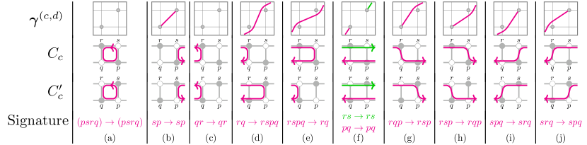
Figure 19. The possible relative cycles and their signatures for the proof in Section 4.3.1.

In Figure 19, we list all possible relative cycles that pass through at least one vertex of the square $psrq$, given together with their monotone curves $\gamma$ inside $\Gamma(u_{(d)})$ and the signatures in $G_{u,\beta}$ and $G_{u,\beta^{\prime}}$. For example, $C_{d}$ is shown in Figure 19(a), and the curve $\gamma$ from Figure 18 is shown in Figure 19(d).

We will want to understand how $C_{c}$ and $C^{\prime}_{c}$ relate, not as drawn in the planar projections in Figure 19, but as drawn on the surface $\mathbf{S}_{u,\beta}=\mathbf{S}_{u,\beta^{\prime}}$. Comparing the signatures to Figure 15, we see that for all $c\in J_{u,\beta}$, the following are equivalent:

• $C_{c}\neq C^{\prime}_{c}$ (as elements of $\Lambda_{u,\beta}=\Lambda_{u,\beta^{\prime}}$);

• either $c=d$ or ${\langle}C_{c},C_{d}{\rangle}>0$ (in which case ${\langle}C_{c},C_{d}{\rangle}=1$);

• $C_{c}$ is shown in Figure 19(a,b,c).

Note that $C_{d}$ is represented in the notation of Figure 15 as the cycle passing through the vertices of the square $psrq$. Thus, in order to have ${\langle}C_{c},C_{d}{\rangle}>0$, when $C_{c}$ is drawn in Figure 15(far left), it needs to start inside $psrq$ and end outside of $psrq$. This happens precisely when $C_{c}$ is one of the relative cycles shown in Figure 19(b,c). We see that indeed in all cases, we have $C^{\prime}_{c}=\mu_{d}(C_{c})$.

Remark 4.4.

In general, $C_{c}$ is represented by a monotone multicurve inside $\Gamma(u_{(d)})$, and thus, for example, the two monotone curves shown in Figure 19(f) could be parts of a single monotone multicurve. However, this does not affect our analysis because the intersection number ${\langle}C_{c},C_{d}{\rangle}$ is additive over all intersection points in $C_{c}\cap C_{d}$.

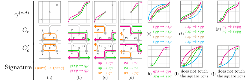
Figure 20. The possible signatures for the proof in Section 4.3.2.

4.3.2. Applying (B3) (fully solid)

We proceed using a similar strategy. Suppose that $i_{d-2}=j$, $i_{d-1}=j+1$, and $i_{d}=j$ for some $j\in I$, with all three indices solid. The 3D plabic graphs $G_{u,\beta}$ and $G_{u,\beta^{\prime}}$ are shown in Figure 17(right). In particular, after applying a contraction-uncontraction move (M1) to the vertices $p_{1},p_{2}$ of $G_{u,\beta}$ and to the vertices $r_{1},r_{2}$ of $G_{u,\beta^{\prime}}$, we obtain two graphs which differ by a square move (M2), where the square has vertices $psrq$. Abusing notation, we denote these two graphs again by $G_{u,\beta}$ and $G_{u,\beta^{\prime}}$.

Let us now classify the relative cycles. There are a total of $26$ options for how a monotone curve can look like inside $\Gamma(u_{(d)})$. In addition, there are $3$ more relative cycles $C_{d}$, $C_{d-1}$, $C_{d-2}$ which do not correspond to any monotone curves in $\Gamma(u_{(d)})$, shown in orange in Figure 20(a,c,d). Out of these $29$ options, $8$ relative cycles shown in Figure 20(i,j) do not pass through any of the vertices of the square $psrq$ (after applying the above contraction-uncontraction moves). The remaining $21$ relative cycles, together with their signatures in $G_{u,\beta}$ and $G_{u,\beta^{\prime}}$, are shown in Figure 20(a–h).

Comparing the signatures to Figure 15, we see that for all $c\in J_{u,\beta}$, the following are equivalent:

• $C_{c}\neq C^{\prime}_{c}$;

• either $c=d$ or ${\langle}C_{c},C_{d}{\rangle}>0$ (in which case ${\langle}C_{c},C_{d}{\rangle}=1$);

• $C_{c}$ is shown in Figure 20(a,b,c).

We again get that $C^{\prime}_{c}=\mu_{d}(C_{c})$ in each case. This completes the proof of part (1) of Theorem 4.3.

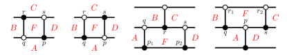
Figure 21. Labeling the faces when applying the square move.

4.3.3. Chamber minors

Suppose we are applying one of the mutation moves from part (1) of Theorem 4.3 at $C_{d}$ for some $d\in J_{u,\beta}^{\operatorname{mut}}$. Then (after possibly applying moves (M1) from Section 4.3.2), the graph $G_{u,\beta}$ contains a square $psrq$. Let $G$ be the portion of the red projection of $G_{u,\beta}$ located in the small neighborhood of $psrq$; thus, $G$ is planar. Let $F$ be the face of $G$ inside this square, and let $A,B,C,D$ be the four faces adjacent to the square in clockwise order; see Figure 21. (We only consider $A,B,C,D$ in a small neighborhood of the square.) For $c\in J_{u,\beta}$ and a face $E\in\{F,A,B,C,D\}$, we will write ${\mathrm{ord}}_{c}(E)=1$ if $E$ is inside $C_{c}$ and ${\mathrm{ord}}_{c}(E)=0$ otherwise. As in Section 2.4, we say that $E$ is inside $C_{c}$ if $E$ is contained inside the red projection of the disk $D_{c}$, or in other words, if $E$ is to the left of the curve representing the red projection of $C_{c}$. We define ${\mathrm{ord}}^{\prime}_{c}(E)$ similarly using the graph $G_{u,\beta^{\prime}}$ and the cycles $C^{\prime}_{c}$ in it. It follows from part (1) of Theorem 4.3 that the difference $C_{c}-C^{\prime}_{c}$ in $\Lambda_{u,\beta}$ is always a multiple of $C_{d}$. Thus, we have ${\mathrm{ord}}^{\prime}_{c}(E)={\mathrm{ord}}_{c}(E)$ for $E\neq F$. (Alternatively, this can be seen directly from Figures 19 and 20.) The following result will be used in the proof of Proposition 8.11.

Lemma 4.5.

For all $c\in J_{u,\beta}\setminus\{d\}$, we have

(4.1) $${\mathrm{ord}}_{c}(F)+{\mathrm{ord}}^{\prime}_{c}(F)=\min({\mathrm{ord}}_{c}(A)+{\mathrm{ord}}_{c}(C),{\mathrm{ord}}_{c}(B)+{\mathrm{ord}}_{c}(D)).$$

Démonstration.

Follows by inspection from Figures 19 and 20. For example, if $C_{c}$ is given in Figure 19(d) then (4.1) becomes $1+0=\min(0+1,1+1)$. Similarly, if both monotone curves in Figure 19(f) are parts of the same monotone multicurve corresponding to $C_{c}$ then (4.1) becomes $0+0=\min(0+0,1+1)$. ∎

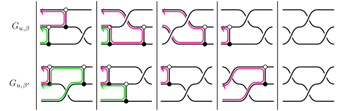
Figure 22. Applying move (B3) (not fully solid).

4.4. Non-mutation moves

We prove part (2) of Theorem 4.3. The following result will be convenient to show equalities of the form $C^{\prime}_{c^{\prime}}=C_{c}$ without classifying all possible monotone curves as we did in Section 4.3.

Lemma 4.6.

Suppose that the double braids $\beta,\beta^{\prime}$ are related by one of the moves (B1)–(B3) involving the indices in some interval $(l,r]\subset[m]$ of length $2$ or $3$. Suppose in addition that the portion $G_{u,\beta}|_{[l,r]}$ of $G_{u,\beta}$ between $\Gamma(u_{(l)})$ and $\Gamma(u_{(r)})$ has no cycles, and that $G_{u,\beta^{\prime}}|_{[l,r]}$ is obtained from $G_{u,\beta}|_{[l,r]}$ via a sequence of contraction-uncontraction moves (M1). Then, for all $c\in J_{u,\beta}\setminus(l,r]$, we have $C_{c}=C^{\prime}_{c}$.

Démonstration.

By Proposition 3.16, the monotone multicurves of $C_{c}$ inside $\Gamma(u_{(l)})$ and $\Gamma(u_{(r)})$ are determined by the combinatorics of almost positive subexpressions, specifically, by the pairs $(u_{(l)},v_{(c)}^{{\langle}l{\rangle}})$ and $(u_{(r)},v_{(c)}^{{\langle}r{\rangle}})$. One can check (cf. Figure 22) that these pairs are invariant under applying the moves (B1)–(B3) on the interval $(l,r]$. Thus, we see that the monotone multicurves of $C_{c}$ inside $\Gamma(u_{(l)})$ and $\Gamma(u_{(r)})$ are preserved under the double braid move. Thus, the locations where $C_{c}$ enters and exits $G_{u,\beta}|_{[l,r]}$ remain unchanged as we apply the move. Since $G_{u,\beta}|_{[l,r]}$ has no cycles, the restriction of $C_{c}$ to $G_{u,\beta}|_{[l,r]}$ is determined by these locations. It is then clear that as we apply the moves (M1) to $G_{u,\beta}|_{[l,r]}$, the relative cycle $C_{c}$ is preserved. ∎

In order to prove part (2) of Theorem 4.3, it suffices to find a relabeling bijection $J_{u,\beta}\xrightarrow{\sim}J_{u,\beta^{\prime}}$, $c\mapsto c^{\prime}$, such that $C^{\prime}_{c^{\prime}}=C_{c}$ for all $c\in J_{u,\beta}$.

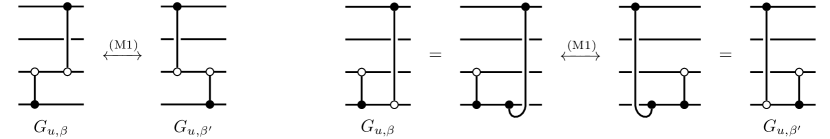
Figure 23. Representing the move (B1) (not special) by the moves from Figure 9.

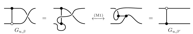
Figure 24. Representing the move (B1) (special, not fully solid) by the moves from Figure 9.

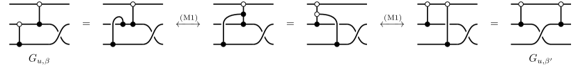
Figure 25. Representing the move (B3) (not fully solid) by the moves from Figure 9.

4.4.1. Applying (B1) (special, not fully solid)

Just as in Section 4.3.1, we assume that we have two crossings $i_{d-1}=-i$ and $i_{d}=j$ (with $i,j\in I$) such that $u_{(d-1)}s_{i}=s_{j}u_{(d-1)}$, but now at least one of the two crossings is hollow. In this case, we must have that $d$ is hollow and $d-1$ is solid. Indeed, recall from (3.1) that $u_{(d-1)}=u_{(d)}\vartriangleleft s_{j}$ and $u_{(d-2)}=s_{i}\vartriangleright u_{(d-1)}$. If $u_{(d-1)}=u_{(d)}s_{j}<u_{(d)}$ then $d$ is hollow, and then $s_{i}u_{(d-1)}=u_{(d-1)}s_{j}=u_{(d)}>u_{(d-1)}$, so $d-1$ must be solid. Otherwise, we have $u_{(d-1)}=u_{(d)}<u_{(d)}s_{j}$, and then $s_{i}u_{(d-1)}=u_{(d-1)}s_{j}>u_{(d-1)}$, so both $d$ and $d-1$ are solid, a contradiction.

After we swap $-i$ and $j$ in $\beta$, the crossing $i^{\prime}_{d}=-i$ becomes hollow while $i^{\prime}_{d-1}=j$ becomes solid. Thus, we have $J_{u,\beta}=J_{u,\beta^{\prime}}$. We take the relabeling bijection to be the identity map. The graphs $G_{u,\beta}$ and $G_{u,\beta^{\prime}}$ are related by a single move (M1) shown in Figure 24, and their restrictions to $[d-2,d]$ have no cycles. By Lemma 4.6, we get $C^{\prime}_{c}=C_{c}$ inside $\Lambda_{u,\beta}=\Lambda_{u,\beta^{\prime}}$ for all $c\in J_{u,\beta}$.

4.4.2. Applying (B1) (not special)

We take the relabeling bijection $c\mapsto c^{\prime}$ to be the transposition of $d-1$ and $d$. If one or both of the crossings $d-1,d$ is hollow, we have $G_{u,\beta}=G_{u,\beta^{\prime}}$, and we check using Lemma 4.6 that $C_{c}=C^{\prime}_{c^{\prime}}$ for all $c\in J_{u,\beta}$. Assume now that both crossings $d-1$ and $d$ are solid.

If the bridges $b_{d-1},b_{d}$ share two strands in common then the move (B1) is special, a contradiction. If the bridges $b_{d-1},b_{d}$ share zero strands in common then $G_{u,\beta}=G_{u,\beta^{\prime}}$, and we are done by Lemma 4.6. From now on, we assume that the bridges $b_{d-1},b_{d}$ share exactly one strand in common.

There are two cases: either the start of one bridge is on the same strand as the end of the other bridge, or the start (resp., the end) of one bridge is on the same strand as the start (resp., the end) of the other bridge. In each case, $G_{u,\beta}$ and $G_{u,\beta^{\prime}}$ are related by a sequence of moves (M1) shown in Figure 23. We are done by Lemma 4.6.

4.4.3. Applying (B2)

We take the relabeling bijection $c\mapsto c^{\prime}$ to be the transposition of $d-1$ and $d$. We have $G_{u,\beta}=G_{u,\beta^{\prime}}$. We are done by Lemma 4.6.

4.4.4. Applying (B3) (not fully solid)

Suppose that $i_{d-2}=j$, $i_{d-1}=j+1$, and $i_{d}=j$ for some $j\in I$. In $\Gamma(u_{(d-3)})$, the dots $(i,j)$, $(i^{\prime},j+1)$, $(i^{\prime\prime},j+2)$ are located in $\prec$-increasing order, i.e., we have $i<i^{\prime}<i^{\prime\prime}$. The restriction of $\Gamma(u_{(d)})$ to the rows $j,j+1,j+2$ and columns $i,i^{\prime},i^{\prime\prime}$, however, could be any permutation in $S_{3}$. If this permutation is the identity, then the crossings $d-2,d-1,d$ are all solid, a contradiction. For each of the remaining five permutations in $S_{3}$, the corresponding graphs $G_{u,\beta}$ and $G_{u,\beta^{\prime}}$ are shown in Figure 22. Observe that their restrictions to $[d-3,d]$ have no cycles. In some cases, we have $G_{u,\beta}=G_{u,\beta^{\prime}}$. In the remaining two cases (one of which is obtained from the other by a vertical flip), the sequence of moves (M1) relating $G_{u,\beta}$ to $G_{u,\beta^{\prime}}$ is shown in Figure 25. In each of the five cases, there is a unique relabeling bijection $J_{u,\beta}\cap\{d-2,d-1,d\}\xrightarrow{\sim}J_{u,\beta^{\prime}}\cap\{d-2,d-1,d\}$ preserving the monotone multicurve inside $\Gamma(u_{(d-3)})$; it is indicated by colored curves in Figure 22. Extending the relabeling bijection by the identity map outside the interval $\{d-2,d-1,d\}$, we are done by Lemma 4.6. This finishes the proof of Theorem 4.3.

4.5. Color-switching moves

We introduce two more moves, which allow us to switch the color of the first or the last letter of $\beta$. For $i\in I=[n-1]$, let $i^{\ast}:=n-i$, so that $s_{i}w_{0}=w_{0}s_{i^{\ast}}$.

1. (assuming $u=w_{0}$) $\beta_{0}i\leftrightarrow\beta_{0}(-i^{\ast})$ for $i\in\pm I$ and $\beta_{0}\in(\pm I)^{m-1}$.

2. $i\beta_{0}\leftrightarrow(-i)\beta_{0}$ for $i\in\pm I$ and $\beta_{0}\in(\pm I)^{m-1}$;

Note that the assumption $u=w_{0}$ in (B4) is not restrictive in view of Remark 3.3.

For an ice quiver $\widetilde{Q}$, its mutable part is the induced subquiver of $\widetilde{Q}$ with vertex set $V^{\operatorname{mut}}$, where $V^{\operatorname{mut}}$ is the set of mutable vertices of $\widetilde{Q}$.

Proposition 4.7.

1. Under the move (B4), $\widetilde{Q}_{u,\beta}$, $G_{u,\beta}$, $\mathbf{S}_{u,\beta}$, and $(C_{c})_{c\in J_{u,\beta}}$ are unchanged.

2. Under the move (B5), the mutable part $Q_{u,\beta}$ of $\widetilde{Q}_{u,\beta}$ is unchanged.

Démonstration.

First, let us consider the move (B4). Since $u=w_{0}$, the index $m$ must be hollow. There are no relative cycles passing through the corresponding strands of $G_{u,\beta}$, since they only pass through the graph $\overline{G}_{u,\beta}$ from Section 3.2. This verifies the first part of the proposition.

Now, consider the move (B5). Without loss of generality, assume that $i:=i_{1}>0$. Since we only care about the mutable part of $\widetilde{Q}_{u,\beta}$, we may disregard all frozen indices, i.e., indices $c\in J_{u,\beta}$ such that the monotone multicurve $\bm{\gamma}^{(c,0)}$ is nonempty. The index $1$ is either hollow or frozen. For any mutable index $d\in J_{u,\beta}$, if $\bm{\gamma}^{(d,1)}$ is empty then the intersection number ${\langle}C_{c},C_{d}{\rangle}$ clearly stays unchanged under (B5) for all $c\in J_{u,\beta}$. Let $c\in J_{u,\beta}$ be a mutable index such that the monotone multicurve $\bm{\gamma}^{(c,1)}$ is nonempty (but $\bm{\gamma}^{(c,0)}$ is empty). Then the index $1$ must be solid (and therefore frozen). Using a contraction-uncontraction move similar to the one in Figure 24, we see that the marked surface $\mathbf{S}_{u,\beta^{\prime}}$ (where $\beta^{\prime}$ is obtained by applying (B5) to $\beta$) is obtained from $\mathbf{S}_{u,\beta}$ by swapping the labels of the marked points $i$ and $i+1$. Since this swap does not affect the part of $\mathbf{S}_{u,\beta}$ to the right of $\Gamma(u_{(0)})$, we see that for any two mutable relative cycles $C_{c},C_{d}$ that pass through the bridge $b_{1}$, their intersection number is unchanged under (B5). This verifies the second part of the proposition. ∎

5. Cluster algebras associated to 3D plabic graphs

The goal of this section is to show that the cluster algebra defined by $\widetilde{Q}_{u,\beta}$ is locally acyclic [Mul13] and really full rank [LS16].

5.1. Background on cluster algebras

We briefly recall the definition of a cluster algebra and related concepts.

Recall from Section 2.3 the definition of an ice quiver $\widetilde{Q}$, with vertex set $\widetilde{V}=V^{\operatorname{mut}}\sqcup V^{\operatorname{fro}}$. We say that $\widetilde{Q}$ is isolated if its mutable part has no arrows. For a set $S\subset V^{\operatorname{mut}}$, let $\widetilde{Q}[S]$ denote the ice quiver obtained from $\widetilde{Q}$ by further declaring all vertices in $S$ to be frozen. We write $\widetilde{Q}-S$ for the ice quiver obtained from $\widetilde{Q}$ by removing the vertices in $S$.

The associated (extended) exchange matrix $\widetilde{B}(\widetilde{Q})=(b_{v,w})_{v\in\widetilde{V},w\in V^{\operatorname{mut}}}$ is defined by

$$b_{v,w}=\#\{\text{arrows $v\to w$ in $\widetilde{Q}$}\}-\#\{\text{arrows $w\to v$ in $\widetilde{Q}$}\}$$

Definition 5.1.

We say that $\widetilde{Q}$ is really full rank if the rows of its exchange matrix span ${\mathbb{Z}}^{|V^{\operatorname{mut}}|}$ over ${\mathbb{Z}}$.

Let $\mathcal{F}\cong{\mathbb{C}}(t_{1},\dots,t_{r})$ be isomorphic to the field of rational functions in $r$ algebraically independent variables. A seed in $\mathcal{F}$ is a pair $\Sigma=({\mathbf{x}},\widetilde{Q})$ where $\widetilde{Q}$ is an ice quiver with $r$ vertices $\widetilde{V}=V^{\operatorname{mut}}\sqcup V^{\operatorname{fro}}$ and ${\mathbf{x}}=\{x_{v}\}_{v\in\widetilde{V}}$ is a transcendence basis of $\mathcal{F}$. The tuple ${\mathbf{x}}$ is the cluster, its elements are cluster variables and $x_{v}$ is mutable if $v\in V^{\operatorname{mut}}$ and frozen otherwise.

Given a seed $({\mathbf{x}},\widetilde{Q})$ in $\mathcal{F}$ and $d\in V^{\operatorname{mut}}$, one can mutate in direction $d$ to obtain a new seed $\mu_{d}({\mathbf{x}},\widetilde{Q})=({\mathbf{x}}^{\prime},\mu_{d}(\widetilde{Q}))$. The quiver of the mutated seed is the mutation of $\widetilde{Q}$ in direction $d$ (see Definition 3.12). The cluster ${\mathbf{x}}^{\prime}=\{x^{\prime}_{v}\}_{v\in\widetilde{V}}$ of the new seed satisfies $x^{\prime}_{v}=x_{v}$ for $v\neq d$ and

$$x^{\prime}_{d}=\frac{\prod_{v\to d}x_{v}+\prod_{d\to v}x_{v}}{x_{d}}\in\mathcal{F}.$$

By repeatedly mutating, we generate (possibly infinitely) many seeds and cluster variables. We denote by ${\mathcal{A}}({\mathbf{x}},\widetilde{Q})$ the cluster algebra associated to the seed $({\mathbf{x}},\widetilde{Q})$. This is the ${\mathbb{C}}$-subalgebra of $\mathcal{F}$ generated by all cluster variables and the inverses of frozen variables. We call ${\mathcal{A}}({\mathbf{x}},\widetilde{Q})$ isolated (resp., really full rank) if $\widetilde{Q}$ is.

We denote by $\mathcal{U}({\mathbf{x}},\widetilde{Q})$ the upper cluster algebra associated to the seed $({\mathbf{x}},\widetilde{Q})$; see [BFZ05]. It is given by

$$\mathcal{U}({\mathbf{x}},\widetilde{Q})=\bigcap_{({\mathbf{x}}^{\prime},\widetilde{Q}^{\prime})}{\mathbb{C}}[(x_{v}^{\prime})^{\pm 1}:v\in\widetilde{V}]\subset\mathcal{F},$$

where the intersection is taken over all seeds $({\mathbf{x}}^{\prime},\widetilde{Q}^{\prime})$ which can be obtained from $({\mathbf{x}},\widetilde{Q})$ by a sequence of mutations.

Note that we have isomorphisms ${\mathcal{A}}({\mathbf{x}},\widetilde{Q})\cong{\mathcal{A}}(\mathbf{y},\widetilde{Q})$ and $\mathcal{U}({\mathbf{x}},\widetilde{Q})\cong\mathcal{U}(\mathbf{y},\widetilde{Q})$ for any two clusters ${\mathbf{x}},\mathbf{y}$. Thus, we may occasionally write ${\mathcal{A}}(\widetilde{Q})$ and $\mathcal{U}(\widetilde{Q})$ if the particular choice of initial cluster does not matter.

In general, we have ${\mathcal{A}}({\mathbf{x}},\widetilde{Q})\subseteq\mathcal{U}({\mathbf{x}},\widetilde{Q})$, and the containment may be strict. However, we have equality if ${\mathcal{A}}({\mathbf{x}},\widetilde{Q})$ is locally acyclic, a property introduced by Muller [Mul13]. We need a few definitions before defining local acyclicity; we follow the presentation of [Mul14].

Let ${\mathcal{A}}({\mathbf{x}},\widetilde{Q})$ be a cluster algebra and let $S\subset V^{\operatorname{mut}}$. Then the cluster algebra ${\mathcal{A}}({\mathbf{x}},\widetilde{Q}[S])$ obtained by freezing $S$ is a cluster localization of ${\mathcal{A}}({\mathbf{x}},\widetilde{Q})$ if

(5.1) $${\mathcal{A}}({\mathbf{x}},\widetilde{Q}[S])={\mathcal{A}}({\mathbf{x}},\widetilde{Q})[x_{v}^{-1}:v\in S].$$

(In general, the left-hand side is contained in the right.) Lemma 4.3 of [Mul13] states that if ${\mathcal{A}}({\mathbf{x}},\widetilde{Q}[S])=\mathcal{U}(x,\widetilde{Q}[S])$, then (5.1) automatically holds.

A collection of cluster localizations $\{{\mathcal{A}}_{i}\}$ of a cluster algebra ${\mathcal{A}}$ is a cover if for every prime ideal $P$ of ${\mathcal{A}}$, there is some ${\mathcal{A}}_{i}$ such that ${\mathcal{A}}_{i}P\subsetneq{\mathcal{A}}_{i}$. A cluster algebra is locally acyclic if it has a cover by isolated cluster algebras. We say that $\widetilde{Q}$ is locally acyclic if ${\mathcal{A}}(\widetilde{Q})$ is.

We will use the following facts about locally acyclic cluster algebras.

Proposition 5.2 ([Mul13, Proposition 3.10]).

Let $\widetilde{Q}$ be an ice quiver and let $Q$ denote its mutable part, as usual. Then ${\mathcal{A}}(\widetilde{Q})$ is locally acyclic if and only if ${\mathcal{A}}(Q)$ is locally acyclic.

Theorem 5.3 ([Mul13, Theorem 4.1]).

If ${\mathcal{A}}({\mathbf{x}},\widetilde{Q})$ is locally acyclic, then ${\mathcal{A}}({\mathbf{x}},\widetilde{Q})=\mathcal{U}({\mathbf{x}},\widetilde{Q})$.

One frequently studied class of locally acyclic quivers are Louise quivers [LS16]. We focus instead on sink-recurrent quivers, defined below, which may not be Louise but are locally acyclic. In the next subsection, we show that our quivers of interest, $\widetilde{Q}_{u,\beta}$, are sink-recurrent (see Theorem 5.6).

Let $Q$ be a quiver with no frozen vertices. A vertex $s$ of $Q$ is a sink if it has no outgoing arrows. We let $N^{\operatorname{in}}_{s}(Q)$ be the set of vertices of $Q$ that have an arrow pointing to $s$. The following notion is analogous to the class of leaf-recurrent quivers from [GL22a, Section 5.4]; see also [GL22a, Remark 5.14].

Definition 5.4.

The class of sink-recurrent quivers is defined recursively as follows.

• Any isolated quiver $Q$ is sink-recurrent.

• Any quiver that is mutation equivalent to a sink-recurrent quiver is sink-recurrent.

• Suppose that a quiver $Q$ has a sink vertex $s$ such that the quivers $Q-\{s\}$ and $Q-(N^{\operatorname{in}}_{s}(Q)\cup\{s\})$ are sink-recurrent. Then $Q$ is sink-recurrent.

The above definition refers to mutable quivers (without frozen vertices). We say that an ice quiver $\widetilde{Q}$ is sink-recurrent if its mutable part $Q$ is sink-recurrent.

Proposition 5.5.

If $\widetilde{Q}$ is a sink-recurrent quiver, then ${\mathcal{A}}({\mathbf{x}},\widetilde{Q})$ is locally acyclic.

Démonstration.

If $\widetilde{Q}$ is isolated, we are done. Otherwise, since local acyclicity is a property of the cluster algebra rather than the quiver, we may assume that $Q$ has a sink $s$ so that $Q-\{s\}$ and $Q-(N^{\operatorname{in}}_{s}(Q)\cup\{s\})$ are sink-recurrent (by mutating if necessary). Consider the freezings ${\mathcal{A}}_{1}={\mathcal{A}}({\mathbf{x}},Q[s])$ and ${\mathcal{A}}_{2}={\mathcal{A}}({\mathbf{x}},Q[N^{\operatorname{in}}_{s}(Q)])$. The mutable parts of $Q[s]$ and $Q[N^{\operatorname{in}}_{s}(Q)]$ are $Q-\{s\}$ and $Q-N^{\operatorname{in}}_{s}(Q)$, respectively, which are both sink-recurrent, the former by definition, and the latter because $Q-N^{\operatorname{in}}_{s}(Q)$ differs from the sink-recurrent quiver $Q-(N^{\operatorname{in}}_{s}(Q)\cup\{t\})$ by an isolated vertex. So ${\mathcal{A}}_{1}$ and ${\mathcal{A}}_{2}$ are locally acyclic by induction, and thus are cluster localizations.

Let $t$ be any neighbor of $s$. Then the pair $(s,t)$ forms a covering pair in the sense of [Mul13], and by [Mul13, Lemma 5.3] it follows that $x_{s}$ and $x_{t}$ cannot simultaneously vanish on ${\mathcal{A}}(\widetilde{Q})$. It follows that ${\mathcal{A}}_{1}$ and ${\mathcal{A}}_{2}$ cover ${\mathcal{A}}$. The union of the covers of ${\mathcal{A}}_{1}$ and ${\mathcal{A}}_{2}$ by isolated cluster algebras is a cover of ${\mathcal{A}}({\mathbf{x}},Q)$ by isolated cluster algebras. ∎

5.2. Local acyclicity

Our goal is to show the following result, which by Proposition 5.5 implies that the cluster algebra ${\mathcal{A}}({\mathbf{x}},\widetilde{Q})$ is locally acyclic.

Theorem 5.6.

For any $u\leq\beta$, the ice quiver $\widetilde{Q}_{u,\beta}$ is sink-recurrent.

Démonstration.

We proceed by induction on the number $\ell(\beta)-\ell(u)$ of vertices of $\widetilde{Q}_{u,\beta}$. For the base case $\ell(\beta)=\ell(u)$, we see that $\beta$ is a reduced word for $u$ and all crossings are hollow, and thus $\widetilde{Q}_{u,\beta}$ is an empty quiver. Let us now assume that $\ell(\beta)>\ell(u)$.

By Remark 3.3, it suffices to consider the case $u=w_{0}$. Applying the moves (B1) and (B4), we may assume that all indices in $\beta$ are positive. Then, assuming $\beta=i\beta_{0}$, we can transform $\beta$ into

(5.2) $$\beta=i\beta_{0}\xrightarrow{\text{{(\hyperref@@ii[bm5]{B\ref*{bm5}})}}}(-i)\beta_{0}\xrightarrow{\text{{(\hyperref@@ii[bm1]{B\ref*{bm1}})}}}\cdots\xrightarrow{\text{{(\hyperref@@ii[bm1]{B\ref*{bm1}})}}}\beta_{0}(-i)\xrightarrow{\text{{(\hyperref@@ii[bm4]{B\ref*{bm4}})}}}\beta_{0}i^{\ast}.$$

We call the operation (5.2) the conjugation move.

Since $u=w_{0}$ and $\ell(\beta)>\ell(u)$, the braid word $\beta$ must be non-reduced. Then, after applying the moves (B2)–(B3), we may transform $\beta$ into a word of the form $\beta_{1}ii\beta_{2}$, for two positive braid words $\beta_{1},\beta_{2}$. Applying conjugation moves (5.2), we may further transform it into the word $ii\beta_{2}\beta_{1}^{\ast}$, where $\beta_{1}^{\ast}$ is obtained from $\beta_{1}$ by applying the map $i\mapsto i^{\ast}$ to each index. Applying one more move (B5), we obtain the word $(-i)i\beta_{2}\beta_{1}^{\ast}$ which we still denote by $\beta$.

By the same argument as in Section 4.4.1, we get that the crossing $i_{1}=-i$ is solid. Let $\beta^{\prime}:=i\beta_{2}\beta_{1}^{\ast}$ be obtained by omitting $-i$ from $\beta$. Since $i_{1}$ is solid, we have $u\leq\beta^{\prime}$, and by the induction hypothesis, the quiver $Q_{u,\beta^{\prime}}$ is sink-recurrent.

Suppose first that the crossing $i_{2}=i$ is hollow. It is easy to check from the propagation rules in Figure 8 that no mutable relative cycle passes through the bridge $b_{1}$. In particular, we see that $Q_{u,\beta}=Q_{u,\beta^{\prime}}$, which we know is sink-recurrent by induction.

Suppose now that both crossings $i_{1}=-i$ and $i_{2}=i$ are solid. The graph $G_{u,\beta}$ has a square $psrq$ formed by the two corresponding bridges as in Figure 15(left). The index $d:=2$ is mutable and the relative cycle $C_{d}$ passes through the vertices of the square in the counterclockwise direction. Any other mutable relative cycle $C_{c}$ satisfying ${\langle}C_{c},C_{d}{\rangle}\neq 0$ must have signature $sp$ (i.e., pass through the bridge $b_{2}$ in the direction opposite to $C_{d}$). In particular, we see that ${\langle}C_{c},C_{d}{\rangle}=1$ whenever $c$ is mutable and ${\langle}C_{c},C_{d}{\rangle}\neq 0$. It follows that $d$ is a sink in $Q_{u,\beta}$.

Let $\beta^{\prime\prime}:=\beta_{2}\beta_{1}^{\ast}$ be obtained by omitting both $-i$ and $i$ from $\beta$. We still have $u\leq\beta^{\prime\prime}$, and by the induction hypothesis, the quiver $Q_{u,\beta^{\prime\prime}}$ is sink-recurrent. We have $Q_{u,\beta^{\prime}}=Q_{u,\beta}-\{d\}$. The quiver $Q_{u,\beta^{\prime\prime}}$ is obtained from $Q_{u,\beta}$ by deleting $d$ together with all vertices that have an arrow pointing to $d$, since the corresponding cycles become frozen in $G_{u,\beta^{\prime\prime}}$. The result follows. ∎

Remark 5.7.

Similar reasoning has been recently used in [GL22a, Proposition 7.9] to study plabic fences, which are recovered as special cases of our construction when $u={\operatorname{id}}$.

From Theorem 5.6 and Proposition 5.5, we have the following immediate corollary.

Corollary 5.8.

For any $u\leq\beta$, the quiver $\widetilde{Q}_{u,\beta}$ is locally acyclic.

5.3. Really full rank

Our goal is to show the following result; cf. Definition 5.1.

Theorem 5.9.

The quiver $\widetilde{Q}_{u,\beta}$ is really full rank.

In order to give a proof, we study the marked surface $(\mathbf{S}_{u,\beta},\mathbf{M})$ and the lattices $\Lambda_{u,\beta}=H_{1}(\mathbf{S}_{u,\beta},\mathbf{M})$ and $\Lambda^{\ast}_{u,\beta}=H_{1}(\mathbf{S}_{u,\beta}\setminus\mathbf{M},\partial\mathbf{S}_{u,\beta}\setminus\mathbf{M})$ in more detail. See Figure 6(d) for an example of a surface $\mathbf{S}_{u,\beta}$. We first construct an explicit basis of $\Lambda^{\ast}_{u,\beta}$. Recall from Section 3.3 that $\mathbf{S}_{u,\beta}$ is obtained by replacing every edge of $G_{u,\beta}$ with a thin rectangle and gluing them together at the vertices of $G_{u,\beta}$. For every edge $e$ of $G_{u,\beta}$, let the dual edge $e^{\ast}\in\Lambda^{\ast}_{u,\beta}$ denote some orientation of a short line segment intersecting $e$ connecting the opposite boundaries of the corresponding thin rectangle.

Lemma 5.10.

The elements $(b^{\ast}_{c})_{c\in J_{u,\beta}}$ form a ${\mathbb{Z}}$-basis of $\Lambda^{\ast}_{u,\beta}$.

Démonstration.

Recall from (3.2) that the lattices $\Lambda_{u,\beta}$ and $\Lambda^{\ast}_{u,\beta}$ are dual to each other. Since $\mathbf{S}_{u,\beta}$ deformation retracts onto $G_{u,\beta}$, we see that $\Lambda_{u,\beta}\cong{\mathbb{Z}}^{|J_{u,\beta}|}$ is a free abelian group whose rank is the number of bridges in $G_{u,\beta}$. Thus, $\Lambda^{\ast}_{u,\beta}\cong{\mathbb{Z}}^{|J_{u,\beta}|}$, and it suffices to show that the elements $(b^{\ast}_{c})_{c\in J_{u,\beta}}$ span $\Lambda^{\ast}_{u,\beta}$ over ${\mathbb{Z}}$.

It is clear that any element of $\Lambda^{\ast}_{u,\beta}$ can be written as a ${\mathbb{Z}}$-linear combination of the elements of the form $e^{\ast}$ for the various edges $e$ of $G_{u,\beta}$: this can be achieved by taking a curve inside $\mathbf{S}_{u,\beta}$ and “pushing it to the boundary,” i.e., applying an isotopy so that the resulting curve is contained inside $\partial\mathbf{S}_{u,\beta}$ with the exception of several line segments of the form $\pm e^{\ast}$ for some edge $e$; see Figure 26. It remains to explain how an arbitrary edge $e^{\ast}$ can be expressed as a ${\mathbb{Z}}$-linear combination of the dual bridge edges.

For any vertex $p$ of $G_{u,\beta}$ incident to edges $e_{1},e_{2},e_{3}$, we have a linear relation $\epsilon_{1}e^{\ast}_{1}+\epsilon_{2}e^{\ast}_{2}+\epsilon_{3}e^{\ast}_{3}=0$ inside $\Lambda^{\ast}_{u,\beta}$, for some $\epsilon_{1},\epsilon_{2},\epsilon_{3}\in\{\pm 1\}$. Every non-bridge edge of $G_{u,\beta}$ passes through a dot inside $\Gamma(u_{(c)})$ for some $c\in[0,m]$. We treat these edges from right to left, i.e., by induction on $c=m,m-1,\dots,0$. For the induction base, if $e$ is a non-bridge edge of $G_{u,\beta}$ whose right endpoint is a degree $1$ vertex in $\Gamma(u_{(m)})$ then clearly $e^{\ast}=0$ in $\Lambda^{\ast}_{u,\beta}$. For the induction step, consider the right endpoint $p$ of $e$, and let $e_{2},e_{3}$ be the other two edges incident to $p$. The above linear relation expresses $e^{\ast}$ as a sum of $\pm e^{\ast}_{2}$ and $\pm e^{\ast}_{3}$, and by the induction hypothesis, each of them is a ${\mathbb{Z}}$-linear combination of dual bridge edges. ∎

Corollary 5.11.

The relative cycles $(C_{c})_{c\in J_{u,\beta}}$ form a ${\mathbb{Z}}$-basis of $\Lambda_{u,\beta}$.

Démonstration.

Each relative cycle $C_{c}$ passes through the bridge edge $b_{c}$ and possibly through some bridges to the left of it. We therefore get ${\langle}C_{c},b^{\ast}_{c}{\rangle}=\pm 1$ and ${\langle}C_{c},b^{\ast}_{d}{\rangle}=0$ for $d>c$. Therefore the matrix ${\langle}C_{c},b^{\ast}_{d}{\rangle}$ is lower triangular with $\pm 1$-s on the diagonal, which implies the result. ∎

Proof of Theorem 5.9.

Our goal is to show that the mutable relative cycles $(C_{c})_{c\in J_{u,\beta}^{\operatorname{mut}}}$ can be extended to a ${\mathbb{Z}}$-basis $\mathcal{B}$ of $\Lambda^{\ast}_{u,\beta}$. Indeed, if this is true, then by Corollary 5.11, each element of the basis of $\Lambda_{u,\beta}$ dual to $\mathcal{B}$ with respect to ${\langle}\cdot,\cdot{\rangle}$ can be expressed as a ${\mathbb{Z}}$-linear combination of $(C_{c})_{c\in J_{u,\beta}}$. This is equivalent to expressing the standard basis vectors of ${\mathbb{Z}}^{k}$, where $k:=|J_{u,\beta}^{\operatorname{mut}}|$, as ${\mathbb{Z}}$-linear combinations of the rows of the exchange matrix $\widetilde{B}(\widetilde{Q}_{u,\beta})$.

We show that $(C_{c})_{c\in J_{u,\beta}^{\operatorname{mut}}}$ can be extended to a ${\mathbb{Z}}$-basis of $\Lambda^{\ast}_{u,\beta}$ by induction in the same way as we did in Theorem 5.6. The ${\mathbb{Z}}$-span of $(C_{c})_{c\in J_{u,\beta}^{\operatorname{mut}}}$ is invariant under mutation formulae (3.4). It is therefore unchanged under the moves (B1)–(B4). For the move (B5), we showed in Proposition 4.7 that the surface $\mathbf{S}_{u,\beta}$ is unchanged except that we swap the labels of two marked points. The collection $(C_{c})_{c\in J_{u,\beta}^{\operatorname{mut}}}$ is also unchanged under (B5). We may therefore apply the moves (B1)–(B5) and arrive at the case where $\beta$ has a double bridge on the left: $\beta=ii\beta_{0}$ for some $\beta_{0}\in(\pm I)^{m-2}$.

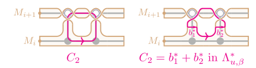
Figure 26. Pushing a relative cycle in $\Lambda^{\ast}_{u,\beta}$ to the boundary.

Let $\beta^{\prime}:=i\beta_{0}$. As in the proof of Theorem 5.6, we have $u\leq\beta^{\prime}$. The graph $G_{u,\beta}$ has one more mutable cycle $C_{d}$ with $d:=2$ and one more bridge $b_{1}$ than the graph $G_{u,\beta^{\prime}}$. Let $\mathcal{B}^{\prime}$ be the ${\mathbb{Z}}$-basis of $\Lambda^{\ast}_{u,\beta^{\prime}}$ containing $(C_{c})_{c\in J_{u,\beta}^{\operatorname{mut}}\setminus\{d\}}$. Then it is clear that $\{b_{1}\}\sqcup\mathcal{B}^{\prime}$ is a ${\mathbb{Z}}$-basis of $\Lambda^{\ast}_{u,\beta}$. As shown in Figure 26, we have $C_{d}=\pm b^{\ast}_{2}\pm b^{\ast}_{1}$ in $\Lambda^{\ast}_{u,\beta}$. Thus, $\mathcal{B}:=\{C_{d}\}\sqcup\mathcal{B}^{\prime}$ is a ${\mathbb{Z}}$-basis of $\Lambda^{\ast}_{u,\beta}$ containing $(C_{c})_{c\in J_{u,\beta}^{\operatorname{mut}}}$. ∎

6. Double braid varieties

6.1. Notation

Let $G=\operatorname{SL}_{n}$. Recall that $I:=[n-1]$ indexes the simple transpositions of the Weyl group $W=S_{n}$, and that for $i\in I$, we denote $i^{*}:=n-i$. For $i\in I$, we set $(-i)^{*}:=-i^{*}$. Let $B_{+}$ and $B_{-}$ denote the subgroup of upper triangular and lower triangular matrices, respectively, and let $U_{+}$ and $U_{-}$ denote the respective unipotent subgroups. We use $H$ to denote the torus of diagonal matrices.

For $i\in I$, let $\phi_{i}:\operatorname{SL}_{2}\to G$ denote the homomorphism where $\phi_{i}(g)$ is the matrix which has $g$ as the $2\times 2$ submatrix on rows and columns $i,i+1$ and otherwise agrees with the identity matrix.

We use $\phi_{i}$ to lift $S_{n}$ to $G$. Let

$$\dot{s}_{i}:=\phi_{i}\begin{pmatrix}0&-1\\ 1&0\end{pmatrix}.$$

For $w\in S_{n}$, we define $\dot{w}:=\dot{s}_{i_{1}}\dots\dot{s}_{i_{n}}$ where $s_{i_{1}}\dots s_{i_{n}}$ is a reduced expression for $w$. The map $w\mapsto\dot{w}$ is not a homomorphism, but if $\ell(vw)=\ell(v)+\ell(w)$, then $(vw)^{\mathchoice{\mathbin{\vbox{\hbox{\scalebox{0.4}{$\displaystyle\bullet$}}}}}{\mathbin{\vbox{\hbox{\scalebox{0.4}{$\textstyle\bullet$}}}}}{\mathbin{\vbox{\hbox{\scalebox{0.4}{$\scriptstyle\bullet$}}}}}{\mathbin{\vbox{\hbox{\scalebox{0.4}{$\scriptscriptstyle\bullet$}}}}}}=\dot{v}\dot{w}$. In particular, $\dot{w}$ does not depend on the choice of reduced expression. Explicitly,

$$(\dot{w})_{i,j}=\begin{cases}0&\text{ if }i\neq w(j),\\ (-1)^{|\{a<j:w(a)>w(j)\}|}&\text{ if }i=w(j).\end{cases}$$

We omit the dot when the choice of the signs in the permutation matrix of $w$ does not matter: e.g., we write $B_{+}wB_{+}$ and $Hw$ in place of $B_{+}\dot{w}B_{+}$ and $H\dot{w}$.

We will also need the generators

(6.1) $$x_{i}(t):=\phi_{i}\begin{pmatrix}1&t\\ 0&1\end{pmatrix},\quad y_{i}(t):=\phi_{i}\begin{pmatrix}1&0\\ t&1\end{pmatrix},\quad\alpha^{\vee}_{i}(t):=\phi_{i}\begin{pmatrix}t&0\\ 0&1/t\end{pmatrix},$$

and the braid matrices

$$z_{i}(t):=\phi_{i}\begin{pmatrix}t&-1\\ 1&0\end{pmatrix}=x_{i}(t)\dot{s}_{i}=\dot{s}_{i}y_{i}(-t);$$

$$\bar{z}_{i}(t):=\phi_{i}\begin{pmatrix}t&1\\ -1&0\end{pmatrix}=x_{i}(-t)\dot{s}^{-1}_{i}=\dot{s}^{-1}_{i}y_{i}(t).$$

6.2. Weighted flags

A weighted flag is an element $F=gU_{+}\in G/U_{+}$. Associated to a weighted flag $F$ is the flag $\pi(F)=gB_{+}$, the image of $F$ in $G/B_{+}$.

Definition 6.1.

Two weighted flags $(F,F^{\prime})$ are called (weakly) $w$-related if there exist $g\in G$ and $h\in H$ such that $(gF,gF^{\prime})=(U_{+},h\dot{w}U_{+})\in G/U_{+}\times G/U_{+}$. Equivalently, $F=g_{1}U_{+}$ and $F^{\prime}=g_{2}U_{+}$ are weakly $w$-related if and only if $g_{1}^{-1}g_{2}\in B_{+}\dot{w}B_{+}$. We write this as $F\stackrel{{\scriptstyle w}}{{\Longrightarrow}}F^{\prime}$.

Two weighted flags $(F,F^{\prime})$ are called strictly $w$-related if there exists $g\in G$ such that $(gF,gF^{\prime})=(U_{+},\dot{w}U_{+})\in G/U_{+}\times G/U_{+}$. Equivalently, $F=g_{1}U_{+}$ and $F^{\prime}=g_{2}U_{+}$ are strictly $w$-related if and only if $g_{1}^{-1}g_{2}\in U_{+}\dot{w}U_{+}$. We write this as $F\stackrel{{\scriptstyle w}}{{\longrightarrow}}F^{\prime}$.

Let $F,F^{\prime}$ be two weighted flags and let $B,B^{\prime}$ be their images in $G/B_{+}$. Then

(6.2) $$F\stackrel{{\scriptstyle w}}{{\longrightarrow}}F^{\prime} F\stackrel{{\scriptstyle w}}{{\Longrightarrow}}F^{\prime} B\stackrel{{\scriptstyle w}}{{\longrightarrow}}B^{\prime}$$ implies , which in turn implies (see Section 2.7).

We collect some elementary facts about relative position (see e.g. [SW21, Appendix]).

Lemma 6.2.

1. $F\stackrel{{\scriptstyle{\operatorname{id}}}}{{\longrightarrow}}F^{\prime}$ if and only if $F=F^{\prime}$.

2. If $F\stackrel{{\scriptstyle v}}{{\longrightarrow}}F^{\prime}\stackrel{{\scriptstyle w}}{{\longrightarrow}}F^{\prime\prime}$ and $\ell(vw)=\ell(v)+\ell(w)$, then $F\stackrel{{\scriptstyle vw}}{{\longrightarrow}}F^{\prime\prime}$.

3. Suppose $\ell(vw)=\ell(v)+\ell(w)$. If $F\stackrel{{\scriptstyle vw}}{{\longrightarrow}}F^{\prime\prime}$, then there exists a unique $F^{\prime}$ such that $F\stackrel{{\scriptstyle v}}{{\longrightarrow}}F^{\prime}$ and $F^{\prime}\stackrel{{\scriptstyle w}}{{\longrightarrow}}F^{\prime\prime}$.

Lemma 6.3.

Suppose $F\stackrel{{\scriptstyle s_{i}}}{{\longrightarrow}}F^{\prime}$ and say $F=gU_{+}$. Then there exists a unique $t\in{\mathbb{C}}$ such that $F^{\prime}=gz_{i}(t)U_{+}$. Similarly, if $F^{\prime}=g^{\prime}U_{+}$, there exists a unique $t^{\prime}\in{\mathbb{C}}$ such that $F=g^{\prime}\bar{z}_{i}(t^{\prime})U_{+}$.

Remark 6.4.

The parameters $t,t^{\prime}$ in Lemma 6.3 depend on the choices of the representative matrices $g,g^{\prime}$.

Lemma 6.5.

Suppose $F\stackrel{{\scriptstyle v}}{{\Longrightarrow}}gU_{+}\stackrel{{\scriptstyle s_{i}}}{{\longrightarrow}}gz_{i}(t)U_{+}$ and let $w$ be such that $F\stackrel{{\scriptstyle w}}{{\Longrightarrow}}gz_{i}(t)U_{+}$. If $vs_{i}>v$, then $w=vs_{i}$ for all $t\in{\mathbb{C}}$. If $vs_{i}<v$, then $w=vs_{i}$ for $t=0$ and $w=v$ for $t\in{{\mathbb{C}}^{\times}}$. In particular, $w\in\{v,vs_{i}\}$.

Lemma 6.6.

Suppose $F\stackrel{{\scriptstyle w}}{{\Longrightarrow}}F^{\prime\prime}$.

1. If $w>ws_{i}$, then there is a unique $F^{\prime}$ such that $F\stackrel{{\scriptstyle ws_{i}}}{{\Longrightarrow}}F^{\prime}\stackrel{{\scriptstyle s_{i}}}{{\longrightarrow}}F^{\prime\prime}$.

2. If $w>s_{i}w$, then there is a unique $F^{\prime}$ such that $F\stackrel{{\scriptstyle s_{i}}}{{\longrightarrow}}F^{\prime}\stackrel{{\scriptstyle s_{i}w}}{{\Longrightarrow}}F^{\prime\prime}$.

Démonstration.

We show only (1). The images $\pi(F)$ and $\pi(F^{\prime\prime})$ in $G/B_{+}$ uniquely determine a flag $L\in G/B_{+}$ satisfying $\pi(F)\stackrel{{\scriptstyle ws_{i}}}{{\longrightarrow}}L\stackrel{{\scriptstyle s_{i}}}{{\longrightarrow}}\pi(F^{\prime\prime})$, and $L$ has a unique lift $F^{\prime}$ to $G/U_{+}$ such that $F^{\prime}\stackrel{{\scriptstyle s_{i}}}{{\longrightarrow}}F^{\prime\prime}$. ∎

6.3. Double braid variety

For a pair $(u,\beta)\in S_{n}\times(\pm I)^{m}$ with $u\leq\beta$, let $\accentset{\circ}{\mathcal{Y}}_{u,\beta}$ denote the space of tuples of weighted flags satisfying

(6.3)

Also define $\mathcal{Y}_{u,\beta}$ by omitting the condition that $(X_{0},Y_{0})$ are weakly $w_{0}$-related. Then $\mathcal{Y}_{u,\beta}$ is a ${\mathbb{C}}^{l}$-bundle over $G/U_{+}$ (where $l=m+\ell(w_{0}u)$), and $\accentset{\circ}{\mathcal{Y}}_{u,\beta}$ is an open subset of $\mathcal{Y}_{u,\beta}$. We denote points in $\accentset{\circ}{\mathcal{Y}}_{{u,\beta}}$ and $\mathcal{Y}_{{u,\beta}}$ by $(X_{\bullet},Y_{\bullet})$.

Remark 6.7.

Intuitively, a point in $\mathcal{Y}_{u,\beta}$ is a walk in $G/U_{+}\times G/U_{+}$ from a pair of weighted flags $X_{m}\stackrel{{\scriptstyle w_{0}u}}{{\longleftarrow}}Y_{m}$ to a pair of weighted flags $X_{0}\stackrel{{\scriptstyle w_{0}}}{{\Longleftarrow}}Y_{0}$. The “direction” of step $c$ is dictated by the crossing $i_{c}$ of $\beta$. A red crossing $i$ in $\beta$ means the step changes the $i$-dimensional subspace of the first flag in the pair. A blue crossing $j$ means the step changes the $(n-|j|)$-dimensional subspace of the second flag. Given an arbitrary pair $(X_{m},Y_{m})$ satisfying $X_{m}\stackrel{{\scriptstyle w_{0}u}}{{\longleftarrow}}Y_{m}$, we can parametrize $(X_{c-1},Y_{c-1})$ iteratively for $c=m,m-1,\dots,1$ using Lemma 6.3: assuming $(X_{c},Y_{c})=(g_{c}U_{+},g^{\prime}_{c}U_{+})$, we set

(6.4) $$(X_{c-1},Y_{c-1}):=\begin{cases}(g_{c}z_{i_{c}}(t_{c})U_{+},g^{\prime}_{c}U_{+}),&\text{if $i_{c}>0$,}\\ (g_{c}U_{+},g^{\prime}_{c}\bar{z}_{|i_{c}|^{*}}(t_{c})U_{+}),&\text{if $i_{c}<0$,}\\ \end{cases}$$

for arbitrary parameters ${\mathbf{t}}:=(t_{1},t_{2},\dots,t_{m})\in{\mathbb{C}}^{m}$. For $(X_{\bullet},Y_{\bullet})$ to be a point in $\accentset{\circ}{\mathcal{Y}}_{u,\beta}$, we require further that $X_{0}\stackrel{{\scriptstyle w_{0}}}{{\Longrightarrow}}Y_{0}$, which is an extra open condition on the parameters $({\mathbf{t}},X_{m},Y_{m})$.

The group $G$ acts on $\accentset{\circ}{\mathcal{Y}}_{u,\beta}$ and $\mathcal{Y}_{u,\beta}$ by acting simultaneously on all the weighted flags by left multiplication.

Proposition 6.8.

The action of $G$ on $\accentset{\circ}{\mathcal{Y}}_{u,\beta}$ is free.

Démonstration.

$G$ acts freely on pairs $(X_{0},Y_{0})$ which are weakly $w_{0}$-related. Indeed, it suffices to consider the case $(X_{0},Y_{0})=(U_{+},h\dot{w}_{0}U_{+})$. The stabilizer of the pair $(U_{+},h\dot{w}_{0}U_{+})$ is $U_{+}\cap h\dot{w}_{0}U_{+}\dot{w}_{0}^{-1}h^{-1}$, which is contained in $U_{+}\cap B_{-}=\{1\}$. ∎

Definition 6.9.

The double braid variety $\accentset{\circ}{R}_{u,\beta}=G\backslash\accentset{\circ}{\mathcal{Y}}_{u,\beta}$ is the quotient of $\accentset{\circ}{\mathcal{Y}}_{u,\beta}$ by $G$.

Our notation is consistent with Section 2 due to the following.

Proposition 6.10.

Let $\beta\in I^{m}$ be a positive braid word. Then the double braid variety $\accentset{\circ}{R}_{{u,\beta}}$ is isomorphic to the braid Richardson variety defined in (2.2).

Démonstration.

Write $\pi$ for the natural map $G/U_{+}\to G/B_{+}$. Let $(X_{\bullet},Y_{\bullet})\in\accentset{\circ}{R}_{{u,\beta}}$. The $G$-action can be gauge-fixed by assuming $(X_{0},Y_{0})=(hU_{+},\dot{w}_{0}U_{+})$, where $h\in H$. With this gauge-fix, we obtain a map $\pi^{m}:\accentset{\circ}{R}_{{u,\beta}}\to(G/B_{+})^{m}$ sending $(X_{\bullet},Y_{\bullet})\mapsto(\pi(X_{1}),\pi(X_{2}),\dots,\pi(X_{m}))$. We now show that this map is an isomorphism onto the braid Richardson variety of (2.2). Since $\pi(X_{0})=B_{+}$ and $\pi(Y_{0})=B_{-}$, (6.2) shows that $\pi^{m}$ maps $\accentset{\circ}{R}_{{u,\beta}}$ into the space (2.2).

For the inverse of $\pi^{m}$: Suppose we have two flags $B,B^{\prime}\in G/B_{+}$ satisfying $B\xrightarrow{s_{i}}B^{\prime}$ and a lift $F\in G/U_{+}$ of $B$ is given. Then there is a unique $F^{\prime}\in G/U_{+}$ that lifts $B^{\prime}$ and satisfies $F\xrightarrow{s_{i}}F^{\prime}$. Now, given a point $B_{\bullet}$ in the space (2.2), we set $Y_{0}=\cdots=Y_{m}=\dot{w_{0}}U_{+}$ and set $X_{m}$ to be the unique lift of $B_{m}$ such that $Y_{m}\stackrel{{\scriptstyle w_{0}u}}{{\longrightarrow}}X_{m}$. Lifting $B_{m-1},B_{m-2},\dots,B_{1}$ from right to left (using the observation at the beginning of the paragraph), we obtain a unique point in $\accentset{\circ}{R}_{{u,\beta}}$ which $\pi^{m}$ maps to $B_{\bullet}$. ∎

Remark 6.11.

When both blue and red subwords of $\beta$ are reduced, the same argument as in the proof of Proposition 6.10 shows that our double braid varieties are isomorphic to the varieties considered by Webster and Yakimov [WY07]. When $u$ is the identity, $\accentset{\circ}{R}_{{\operatorname{id}},\beta}$ is isomorphic to the double Bott–Samelson cells of Shen and Weng [SW21].

Remark 6.12.

The isomorphism of Proposition 6.10 is not compatible with total positivity, in the sense that it does not send the totally positive part $R_{u,w}^{>0}$ of $\accentset{\circ}{R}_{u,w}$ (introduced by Lusztig [Lus94]) to the subset of the braid variety $\accentset{\circ}{R}_{u,{\mathbf{w}}}$ where all cluster variables take positive value. In order to fix that, one must compose this isomorphism with an automorphism of $\accentset{\circ}{R}_{u,w}$ discussed in Section 6.6.

Notation 6.13.

For any object defined in terms of a pair $(u,\beta)$, we suppress the permutation $u$ from the notation when $u=w_{0}$. For example, we write $\accentset{\circ}{R}_{\beta}:=\accentset{\circ}{R}_{w_{0},\beta}$.

Lemma 6.14.

Given $u\leq\beta$, let $\gamma^{+}\in I^{\ell(w_{0}u)}$ be a reduced word for $w_{0}u$ using red letters and $\gamma^{-}\in(-I)^{\ell(uw_{0})}$ be a reduced word for $uw_{0}$ in blue letters. Then

$$\accentset{\circ}{\mathcal{Y}}_{u,\beta}\cong\accentset{\circ}{\mathcal{Y}}_{\beta\gamma^{+}}\cong\accentset{\circ}{\mathcal{Y}}_{\beta\gamma^{-}}\quad\text{and}\quad\accentset{\circ}{R}_{u,\beta}\cong\accentset{\circ}{R}_{\beta\gamma^{+}}\cong\accentset{\circ}{R}_{\beta\gamma^{-}}.$$

Démonstration.

The isomorphisms

$$\accentset{\circ}{\mathcal{Y}}_{\beta\gamma^{+}}\to\accentset{\circ}{\mathcal{Y}}_{u,\beta}\qquad\accentset{\circ}{\mathcal{Y}}_{\beta\gamma^{-}}\to\accentset{\circ}{\mathcal{Y}}_{u,\beta}$$

are given by truncating $(X_{\bullet},Y_{\bullet})$ after the pair $(X_{\ell(\beta)},Y_{\ell(\beta)})$. The choice of $\gamma^{+}$ and $\gamma^{-}$ together with Lemma 6.2(2) ensures that the maps are well defined. Injectivity and surjectivity follow from Lemma 6.2(3). The isomorphisms are $G$-equivariant and so descend to the quotient. ∎

6.4. Geometry of double braid varieties

Proposition 6.15.

For $u\leq\beta$, the double braid variety $\accentset{\circ}{R}_{{u,\beta}}$ is a smooth, affine, irreducible complex algebraic variety of dimension equal to $d(u,\beta):=\ell(\beta)-\ell(u)$.

Démonstration.

Using Lemma 6.14, we may assume $u=w_{0}$. Consider the space of tuples of weighted flags satisfying

(6.5)

This space is an iterated ${\mathbb{C}}^{1}$-bundle and thus affine. Imposing the condition that $U_{+}$ and $Y_{0}$ are weakly $w_{0}$-related (that is, $Y_{0}\in B_{+}\dot{w}_{0}B_{+}=B_{+}\dot{w}_{0}U_{+}$) cuts out a nonempty smooth affine open subset $V$ of the iterated ${\mathbb{C}}^{1}$-bundle. The braid variety $\accentset{\circ}{R}_{\beta}$ is the quotient of $V$ by the diagonal action of $U_{+}=\text{Stab}_{G}(U_{+})$. The group $U_{+}$ acts freely on $B_{+}\dot{w}_{0}U_{+}$ and thus acts freely on $V$. It follows that the quotient $\accentset{\circ}{R}_{\beta}$ is also smooth and affine; it is also clearly irreducible.

For the dimension, note that

$$\dim(\accentset{\circ}{\mathcal{Y}}_{\beta})=\dim(G/U_{+})+\ell(\beta)=\dim(G)-\ell(w_{0})+\ell(\beta)$$

so $\dim(\accentset{\circ}{R}_{\beta})=\dim(\accentset{\circ}{\mathcal{Y}}_{\beta})-\dim(G)=\ell(\beta)-\ell(w_{0})$. ∎

Proposition 6.16.

Let $u\leq\beta$. Suppose that $\beta^{\prime}$ is related to $\beta$ by any of the moves (B1)–(B5). Then $\accentset{\circ}{R}_{{u,\beta}}\cong\accentset{\circ}{R}_{u,\beta^{\prime}}$.

Démonstration.

Using Lemma 6.14, we assume that $u=w_{0}$. We give an isomorphism $m:\accentset{\circ}{\mathcal{Y}}_{\beta}\to\accentset{\circ}{\mathcal{Y}}_{\beta^{\prime}}$, which is $G$-equivariant and so descends to an isomorphism of double braid varieties. The map $m$ changes only the weighted flags indexed by letters involved in the double braid or color-changing move, so we show only that snippet of the tuple. For moves involving letters of a single color, we give the isomorphism for the “red” move; the isomorphism is similar for the “blue” move. Without loss of generality, we may use the action of $G$ to gauge-fix one of the weighted flags involved to be $U_{+}$.

For (B1) ($ij\mapsto ji$ with $i,j$ of opposite color), the map $m$ is given by

$$\left(\leavevmode\hbox to104.12pt{\vbox to56.91pt{\text{[drawing]}}}\right)\mapsto\left(\leavevmode\hbox to104.82pt{\vbox to56.91pt{\text{[drawing]}}}\right). {X} {X^{\prime}} {X^{\prime}} {Y} {Y} {Y^{\prime}} \scriptstyle{{\color[rgb]{1,0,0}s_{i}}} \scriptstyle{{\color[rgb]{1,0,0}{\operatorname{id}}}} \scriptstyle{{\color[rgb]{0,0,1}{\operatorname{id}}}} \scriptstyle{{\color[rgb]{0,0,1}s_{j^{\ast}}}} {X} {X} {X^{\prime}} {Y} {Y^{\prime}} {Y^{\prime}.} \scriptstyle{{\color[rgb]{1,0,0}{\operatorname{id}}}} \scriptstyle{{\color[rgb]{1,0,0}s_{i}}} \scriptstyle{{\color[rgb]{0,0,1}s_{j^{\ast}}}} \scriptstyle{{\color[rgb]{0,0,1}{\operatorname{id}}}} {X} {X^{\prime}} {X^{\prime}} {Y} {Y} {Y^{\prime}} \scriptstyle{{\color[rgb]{1,0,0}s_{i}}} \scriptstyle{{\color[rgb]{1,0,0}{\operatorname{id}}}} \scriptstyle{{\color[rgb]{0,0,1}{\operatorname{id}}}} \scriptstyle{{\color[rgb]{0,0,1}s_{j^{\ast}}}} {X} {X} {X^{\prime}} {Y} {Y^{\prime}} {Y^{\prime}.} \scriptstyle{{\color[rgb]{1,0,0}{\operatorname{id}}}} \scriptstyle{{\color[rgb]{1,0,0}s_{i}}} \scriptstyle{{\color[rgb]{0,0,1}s_{j^{\ast}}}} \scriptstyle{{\color[rgb]{0,0,1}{\operatorname{id}}}}$$

For (B2) ($ij\mapsto ji$ with $i,j$ of the same color, $|i-j|>1$), we use the identity $z_{i}(t_{1})z_{j}(t_{2})=z_{j}(t_{2})z_{i}(t_{1})$. Supposing that the move is on red letters, the map $m$ sends

$$\leavevmode\hbox to185.01pt{\vbox to19.42pt{\text{[drawing]}}}\mapsto\leavevmode\hbox to184.31pt{\vbox to19.42pt{\text{[drawing]}}} {\big{(}z_{j}(t_{2})z_{i}(t_{1})U_{+}} {z_{j}(t_{2})U_{+}} {U_{+}\big{)}} \scriptstyle{{\color[rgb]{1,0,0}s_{i}}} \scriptstyle{{\color[rgb]{1,0,0}s_{j}}} {\big{(}z_{i}(t_{1})z_{j}(t_{2})U_{+}} {z_{i}(t_{1})U_{+}} {U_{+}\big{)}} \scriptstyle{{\color[rgb]{1,0,0}s_{j}}} \scriptstyle{{\color[rgb]{1,0,0}s_{i}}} {\big{(}z_{j}(t_{2})z_{i}(t_{1})U_{+}} {z_{j}(t_{2})U_{+}} {U_{+}\big{)}} \scriptstyle{{\color[rgb]{1,0,0}s_{i}}} \scriptstyle{{\color[rgb]{1,0,0}s_{j}}} {\big{(}z_{i}(t_{1})z_{j}(t_{2})U_{+}} {z_{i}(t_{1})U_{+}} {U_{+}\big{)}} \scriptstyle{{\color[rgb]{1,0,0}s_{j}}} \scriptstyle{{\color[rgb]{1,0,0}s_{i}}}$$

and does not affect the weighted flags in the bottom row.

For (B3) ($iji\mapsto jij$ with $i,j$ of the same sign, $j=i+1$), we use the identity $z_{i}(t_{1})z_{i+1}(t_{2})z_{i}(t_{3})=z_{i+1}(t_{3})z_{i}(t_{1}t_{3}-t_{2})z_{i+1}(t_{1})$. Supposing that the move is on red letters, the map $m$ sends

$$\mapsto\leavevmode\hbox to357.5pt{\vbox to19.42pt{\text{[drawing]}}} {\big{(}z_{i+1}(t_{3})z_{i}(t_{1}t_{3}-t_{2})z_{i+1}(t_{1})U_{+}} {z_{i+1}(t_{3})z_{i}(t_{1}t_{3}-t_{2})U_{+}} {z_{i+1}(t_{3})U_{+}} {U_{+}\big{)}} \scriptstyle{{\color[rgb]{1,0,0}s_{i+1}}} \scriptstyle{{\color[rgb]{1,0,0}s_{i}}} \scriptstyle{{\color[rgb]{1,0,0}s_{i+1}}} {\big{(}z_{i+1}(t_{3})z_{i}(t_{1}t_{3}-t_{2})z_{i+1}(t_{1})U_{+}} {z_{i+1}(t_{3})z_{i}(t_{1}t_{3}-t_{2})U_{+}} {z_{i+1}(t_{3})U_{+}} {U_{+}\big{)}} \scriptstyle{{\color[rgb]{1,0,0}s_{i+1}}} \scriptstyle{{\color[rgb]{1,0,0}s_{i}}} \scriptstyle{{\color[rgb]{1,0,0}s_{i+1}}}$$

and does not affect weighted flags in the bottom row.

For (B4) ($\beta i\mapsto\beta(-i^{\ast})$ assuming $u=w_{0}$), we have $X_{m}=Y_{m}$. We note that $(i^{\ast})^{\ast}=i$. The map $m$ is given by

$$\left(\leavevmode\hbox to62.44pt{\vbox to56.28pt{\text{[drawing]}}}\right)\mapsto\left(\leavevmode\hbox to60.9pt{\vbox to54.2pt{\text{[drawing]}}}\right). {X} {X^{\prime}} {X^{\prime}} {X^{\prime}} \scriptstyle{{\color[rgb]{1,0,0}s_{i}}} \scriptstyle{{\color[rgb]{0,0,1}{\operatorname{id}}}} {X} {X} {X^{\prime}} {X} \scriptstyle{{\color[rgb]{1,0,0}{\operatorname{id}}}} \scriptstyle{{\color[rgb]{0,0,1}s_{i}}} {X} {X^{\prime}} {X^{\prime}} {X^{\prime}} \scriptstyle{{\color[rgb]{1,0,0}s_{i}}} \scriptstyle{{\color[rgb]{0,0,1}{\operatorname{id}}}} {X} {X} {X^{\prime}} {X} \scriptstyle{{\color[rgb]{1,0,0}{\operatorname{id}}}} \scriptstyle{{\color[rgb]{0,0,1}s_{i}}}$$

For (B5) ($(-i)\beta\mapsto i\beta$), we use the identity $z_{i^{*}}(t)^{-1}h\dot{w}_{0}=h^{\prime}\dot{w}_{0}\bar{z}_{i}(t^{\prime})$, where $t^{\prime}=th_{i^{*}+1}/h_{i^{*}}$ and $h^{\prime}_{j,j}=h_{s_{i^{*}}(j),s_{i^{*}}(j)}$. Assuming $i\in I$, the map $m$ sends

$$\left(\leavevmode\hbox to137.8pt{\vbox to62.96pt{\text{[drawing]}}}\right)\mapsto\left(\leavevmode\hbox to111.39pt{\vbox to59.44pt{\text{[drawing]}}}\right).\qed {z_{i^{*}}(t)^{-1}h\dot{w}_{0}U_{+}} {z_{i^{*}}(t)^{-1}h\dot{w}_{0}U_{+}} {z_{i^{*}}(t)^{-1}U_{+}} {U_{+}} \scriptstyle{{\color[rgb]{1,0,0}{\operatorname{id}}}} \scriptstyle{{\color[rgb]{0,0,1}s_{i^{\ast}}}} \scriptstyle{w_{0}} {h^{\prime}\dot{w}_{0}U_{+}} {h^{\prime}\dot{w}_{0}\bar{z}_{i}(t^{\prime})U_{+}} {U_{+}} {U_{+}} \scriptstyle{{\color[rgb]{1,0,0}s_{i}}} \scriptstyle{w_{0}} \scriptstyle{{\color[rgb]{0,0,1}{\operatorname{id}}}} {z_{i^{*}}(t)^{-1}h\dot{w}_{0}U_{+}} {z_{i^{*}}(t)^{-1}h\dot{w}_{0}U_{+}} {z_{i^{*}}(t)^{-1}U_{+}} {U_{+}} \scriptstyle{{\color[rgb]{1,0,0}{\operatorname{id}}}} \scriptstyle{{\color[rgb]{0,0,1}s_{i^{\ast}}}} \scriptstyle{w_{0}} {h^{\prime}\dot{w}_{0}U_{+}} {h^{\prime}\dot{w}_{0}\bar{z}_{i}(t^{\prime})U_{+}} {U_{+}} {U_{+}} \scriptstyle{{\color[rgb]{1,0,0}s_{i}}} \scriptstyle{w_{0}} \scriptstyle{{\color[rgb]{0,0,1}{\operatorname{id}}}}$$

From Lemma 6.14 and Proposition 6.16, we have an immediate corollary.

Corollary 6.17.

Any double braid variety $\accentset{\circ}{R}_{{u,\beta}}$ with $u\leq\beta$ is isomorphic to a braid variety $\accentset{\circ}{R}_{\beta^{\prime}}$ where $\beta^{\prime}$ has only red letters.

The purpose of defining double braid varieties is to obtain more seeds (or more Deodhar tori), one for each double braid word.

6.5. Grid and chamber minors

We next discuss regular functions on $\accentset{\circ}{R}_{{u,\beta}}$. Given $(X_{\bullet},Y_{\bullet})$, let

(6.6) $$Z_{c}:=Y_{c}^{-1}X_{c}\in U_{+}\backslash G/U_{+}.$$

It is clear that $Z_{c}$ is well defined for a point in $\accentset{\circ}{R}_{{u,\beta}}$, since it is unchanged by the action of $G$. We frequently abuse notation and use $Z_{c}$ to denote both the double coset and a representative of this double coset. Our goal is to use the matrix $Z_{c}$ to introduce certain regular functions on $\accentset{\circ}{R}_{u,\beta},\accentset{\circ}{\mathcal{Y}}_{u,\beta},\mathcal{Y}_{u,\beta}$ which we refer to as grid minors. Recall from Section 3.1 the definition of the $u$-PDS ${\mathbf{u}}=(u_{(0)},\dots,u_{(m)})$.

Definition 6.18.

For $c\in J_{u,\beta}$ a crossing and $h\in I$, we define the red grid minor as

(6.7) $$\Delta_{c,h}(X_{\bullet},Y_{\bullet})=\Delta_{w_{0}u_{(c)}[h],[h]}(Z_{c}),$$

and the blue grid minor as

(6.8) $$\Delta_{c,-h}(X_{\bullet},Y_{\bullet})=\Delta_{[n+1-h,n],u_{(c)}^{-1}w_{0}[n+1-h,n]}(Z_{c})=\Delta_{w_{0}[h],u_{(c)}^{-1}[h]}(Z_{c}),$$

where $Z_{c}=Y_{c}^{-1}X_{c}$.

Note that the color of a grid minor $\Delta_{c,h}$ is determined by the sign of $h$. It is not true in general that for $J\subset[n]$ of size $|J|=h$, a flag minor of the form $\Delta_{J,[h]}$ or $\Delta_{w_{0}[h],J}$ gives a well-defined function on $U_{+}\backslash G/U_{+}$. However, for the particular varieties we are interested in, grid minors indeed give rise to well-defined functions.

Lemma 6.19.

For each $c\in J_{u,\beta}$ and $h\in I$, the grid minors $\Delta_{c,\pm h}$ give rise to $G$-invariant regular functions on $\mathcal{Y}_{u,\beta}$ and $\accentset{\circ}{\mathcal{Y}}_{u,\beta}$, and to regular functions on $\accentset{\circ}{R}_{u,\beta}$. These regular functions are compatible with the quotient map $\accentset{\circ}{\mathcal{Y}}_{u,\beta}\to\accentset{\circ}{R}_{u,\beta}$ and the inclusion map $\accentset{\circ}{\mathcal{Y}}_{u,\beta}\hookrightarrow\mathcal{Y}_{u,\beta}$.

Démonstration.

As we will explain in Section 7, each of $\accentset{\circ}{R}_{u,\beta},\accentset{\circ}{\mathcal{Y}}_{u,\beta},\mathcal{Y}_{u,\beta}$ contains an open dense subset consisting of $(X_{\bullet},Y_{\bullet})$ satisfying $X_{c}\stackrel{{\scriptstyle w_{0}u_{(c)}}}{{\Longleftarrow}}Y_{c}$ for all $c\in[0,m]:=\{0,1,\dots,m\}$. In this case, $Z_{c}$ is contained in a specific Bruhat cell $\accentset{\circ}{\mathcal{X}}_{w_{0}u_{(c)}}:=B_{+}w_{0}u_{(c)}B_{+}$ of $G$. Therefore for arbitrary $(X_{\bullet},Y_{\bullet})$, $Z_{c}$ belongs to the closure $\mathcal{X}_{w_{0}u_{(c)}}$ of $\accentset{\circ}{\mathcal{X}}_{w_{0}u_{(c)}}$ inside $G$. It is well known that the flag minors of the form (6.7)–(6.8) give rise to $U_{+}\times U_{+}$-invariant regular functions on $\mathcal{X}_{w_{0}u_{(c)}}$, which are moreover nonvanishing on $\accentset{\circ}{\mathcal{X}}_{w_{0}u_{(c)}}$. Explicitly, each matrix in $\accentset{\circ}{\mathcal{X}}_{w_{0}u_{(c)}}$ can be transformed by the $U_{+}\times U_{+}$-action into a unique matrix in the torus $w_{0}u_{(c)}H$, and the grid minors are characters of this torus. The fact that these functions are $G$-invariant and compatible with the quotient/inclusion maps is obvious from the definition of $Z_{c}$. ∎

Lemma 6.20.

Consider a crossing $c\in[m]$. Suppose $h\neq i_{c}$ is of the same sign as $i_{c}$. Then

$$\Delta_{c-1,h}=\Delta_{c,h}.$$

Démonstration.

Let $i:=i_{c}$. The result follows from the fact that $Z_{c-1}=Z_{c}x_{i}(t)\dot{s}_{i}$ or $Z_{c-1}=\dot{s}_{i^{*}}x_{i^{*}}(t)Z_{c}$ (as usual using $Z_{c}$ also to denote a representative for the double coset) for some $t\in{\mathbb{C}}$, depending on whether $c$ is red or blue. ∎

We will be particularly interested in the following subclass of grid minors.

Definition 6.21.

Define the chamber minor of $c$ as

(6.9) $$\Delta_{c}:=\Delta_{c-1,i_{c}}.$$

Note that $\Delta_{c}$ is a minor of $Z_{c-1}$. In words, Lemma 6.20 shows that a crossing of color $x\in\{\text{red},\text{blue}\}$ can change exactly one grid minor of color $x$ (but may change many grid minors of the opposite color). The “changed” grid minor of color $x$ to the left of the bridge $b_{c}$ is exactly the chamber minor $\Delta_{c}$.

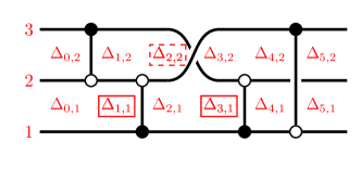
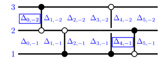
(a) $\pi_{\operatorname{red}}(G_{u,\beta})$, red grid minors (labels) (b) $\pi_{\operatorname{blue}}(G_{u,\beta})$, blue grid minors (labels)

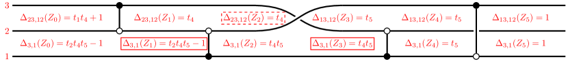
(c) $\pi_{\operatorname{red}}(G_{u,\beta})$, red grid minors (values)

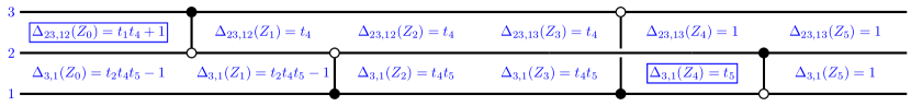
(d) $\pi_{\operatorname{blue}}(G_{u,\beta})$, blue grid minors (values)

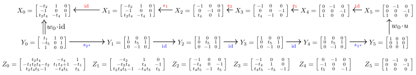
(e) the matrices $X_{c},Y_{c},Z_{c}$ for $c\in[0,m]$

Figure 27. Grid minors for $u=s_{2}$ and $\beta=(-2,1,2,1,-1)$; see Example 3.10, Figure 6, and Example 6.24. The chamber minors $\Delta_{c}$, $c\in[m]$, are boxed.

Remark 6.22.

We explain the relationship between grid minors and 3D plabic graphs; compare Figure 27 to Figure 6. Recall from Section 3.2 that for a 3D plabic graph $G_{u,\beta}$ with coordinates $(i,j,t)$, we consider its red projection $\pi_{\operatorname{red}}(G_{u,\beta})$ with coordinates $(t,j)$ and its blue projection $\pi_{\operatorname{blue}}(G_{u,\beta})$ with coordinates $(t,i)$. For $c\in[0,m]$ and $h\in I$, let us place the red grid minor $\Delta_{c,h}$ at the point $(t=c,j=h+0.5)$, lying in some face of $\pi_{\operatorname{red}}(G_{u,\beta})$. Similarly, we place the blue grid minor $\Delta_{c,-h}$ at the point $(t=c,i=h+0.5)$, lying in some face of $\pi_{\operatorname{blue}}(G_{u,\beta})$. This labeling is shown in Figure 27(a,b). Each chamber minor $\Delta_{c}$ appears immediately to the left of the bridge $b_{c}$ in the projection of the corresponding color; these minors are boxed in Figure 27.

Remark 6.23.

Lemma 6.20 can be seen as a special case of the observation that any two red (resp., blue) grid minors that belong to the same face of $\pi_{\operatorname{red}}(G_{u,\beta})$ (resp., $\pi_{\operatorname{blue}}(G_{u,\beta})$) are equal.

Example 6.24.

We continue Example 3.10; thus, $u=s_{2}$, $\beta=(-2,1,2,1,-1)$, and $J_{u,\beta}=\{1,2,4,5\}$. The matrices $X_{c},Y_{c},Z_{c}$ are computed in Figure 27(e) from right to left using (6.4). The grid minors given by (6.7)–(6.8) are computed in Figure 27(c,d). The solid (resp., hollow) chamber minors are boxed in solid (resp., dashed) lines.

6.6. Comparison with chamber minors for Richardsons and double Bruhat cells

As we mentioned in the introduction, braid varieties include double Bruhat cells, open positroid varieties, and open Richardson varieties, cluster structures on which have been studied previously in many works including [FZ99, GY20, Sco06, SSBW19, GL19, Lec16, Ing19]. We briefly explain how our chamber minors relate to chamber minors defined in some of these previous works.

Let $g\mapsto g^{-\iota}$ be the involutive automorphism of $G$ defined by

$$x_{i}(t)\mapsto x_{i}(-t),\quad y_{i}(t)\mapsto y_{i}(-t),\quad\dot{s}_{i}\mapsto\dot{s}_{i}^{-1},\quad h\mapsto h,$$

for all $i\in I$, $t\in{\mathbb{C}}$, and $h\in H$. This map is a composition of the involution $g\mapsto g^{\iota}$ studied in [FZ99, Section 2.1] with the involution $g\mapsto g^{-1}$ (these two involutions commute). The properties of the involution $g\mapsto g^{-\iota}$ in relation to total positivity were first studied in [GL22b, Section 6.2]. Since $G=\operatorname{SL}_{n}$, one can check that for a matrix $g=(g_{i,j})_{i,j\in[n]}$, we have $g^{-\iota}=((-1)^{i+j}g_{i,j})_{i,j\in[n]}$.

We will use the following relations for relative positions of weighted flags:

(6.10) $$U_{+}\stackrel{{\scriptstyle{\color[rgb]{1,0,0}s_{i}}}}{{\longleftarrow}}\dot{s}_{i}^{-1}U_{+},\quad\alpha^{\vee}_{i}(1/t)U_{+}\stackrel{{\scriptstyle{\color[rgb]{1,0,0}s_{i}}}}{{\longleftarrow}}y_{i}(-t)U_{+},\quad\alpha^{\vee}_{i^{\ast}}(t)\dot{w}_{0}^{-1}U_{+}\stackrel{{\scriptstyle{\color[rgb]{0,0,1}s_{i^{\ast}}}}}{{\longrightarrow}}x_{i^{\ast}}(-t)\dot{w}_{0}^{-1}U_{+},$$

for all $t\in{{\mathbb{C}}^{\times}}$ and $i\in I$, where $\alpha^{\vee}_{i}$ was defined in (6.1).

6.6.1. Open Richardson varieties

Observe that the map $gB_{+}\mapsto g^{-\iota}B_{+}$ preserves the subsets $B_{-}uB_{+}$, $B_{+}wB_{+}$, and therefore yields an involutive automorphism of $\accentset{\circ}{R}_{u,w}$. Choose a reduced word $\beta$ for $w$ and consider the isomorphism between an open Richardson and a braid Richardson variety

(6.11) $$\accentset{\circ}{R}_{u,w}\xrightarrow{\sim}\accentset{\circ}{R}_{{u,\beta}},\quad gB_{+}\mapsto(X_{\bullet},Y_{\bullet}),$$

where $(X_{\bullet},Y_{\bullet})$ satisfies the following conditions:

$$\pi(X_{0})=B_{+},\quad\pi(X_{m})=g^{-\iota}B_{+},\quad\text{and}\quad Y_{0}=Y_{1}=\cdots=Y_{m}=\dot{w}_{0}^{-1}U_{+}.$$

As explained in the proof of Proposition 6.10, these conditions determine the tuple $(X_{\bullet},Y_{\bullet})\in\accentset{\circ}{R}_{{u,\beta}}$ uniquely. We explain how to do this explicitly when the element $gB_{+}$ is MR-parametrized; such parametrizations were introduced in [MR04] in relation to total positivity for flag varieties [Lus94]. Let

(6.12) $$g:=g_{1}\cdots g_{m},\qquad\text{where}\qquad g_{c}=\begin{cases}\dot{s}_{i_{c}}&\mbox{if $c\notin J_{u,\beta}$,}\\ y_{i_{c}}(t_{c})&\mbox{if $c\in J_{u,\beta}$.}\end{cases}$$

Here ${\mathbf{t}}=(t_{1},\dots,t_{m})$ consists of some nonzero parameters. We get

$$g^{-\iota}=g_{1}^{-\iota}\cdots g_{m}^{-\iota},\qquad\text{where}\qquad g_{c}^{-\iota}=\begin{cases}\dot{s}_{i_{c}}^{-1}&\mbox{if $c\notin J_{u,\beta}$,}\\ y_{i_{c}}(-t_{c})&\mbox{if $c\in J_{u,\beta}$.}\end{cases}$$

We first check that we may set $X_{m}:=g^{-\iota}U_{+}$, i.e., that $X_{m}\stackrel{{\scriptstyle w_{0}u}}{{\longleftarrow}}Y_{m}$. Indeed, it is well known [GL22b, Equation (2.8)] that $g\in U_{-}\dot{u}$. Thus, $g^{-\iota}\in U_{-}\ddot{u}$, where for a reduced word $u=s_{j_{1}}\cdots s_{j_{l}}$, we set $\ddot{u}:=\dot{u}^{-\iota}=((u^{-1})^{\mathchoice{\mathbin{\vbox{\hbox{\scalebox{0.4}{$\displaystyle\bullet$}}}}}{\mathbin{\vbox{\hbox{\scalebox{0.4}{$\textstyle\bullet$}}}}}{\mathbin{\vbox{\hbox{\scalebox{0.4}{$\scriptstyle\bullet$}}}}}{\mathbin{\vbox{\hbox{\scalebox{0.4}{$\scriptscriptstyle\bullet$}}}}}})^{-1}=\dot{s}_{j_{1}}^{-1}\cdots\dot{s}_{j_{l}}^{-1}$. The element $\ddot{u}$ satisfies $\dot{w}_{0}\ddot{u}=(w_{0}u)^{\mathchoice{\mathbin{\vbox{\hbox{\scalebox{0.4}{$\displaystyle\bullet$}}}}}{\mathbin{\vbox{\hbox{\scalebox{0.4}{$\textstyle\bullet$}}}}}{\mathbin{\vbox{\hbox{\scalebox{0.4}{$\scriptstyle\bullet$}}}}}{\mathbin{\vbox{\hbox{\scalebox{0.4}{$\scriptscriptstyle\bullet$}}}}}}$. It follows that $\dot{w}_{0}\cdot(X_{m},Y_{m})=(\dot{w}_{0}g^{-\iota}U_{+},U_{+})$, where $\dot{w}_{0}g^{-\iota}U_{+}\in U_{+}(w_{0}u)^{\mathchoice{\mathbin{\vbox{\hbox{\scalebox{0.4}{$\displaystyle\bullet$}}}}}{\mathbin{\vbox{\hbox{\scalebox{0.4}{$\textstyle\bullet$}}}}}{\mathbin{\vbox{\hbox{\scalebox{0.4}{$\scriptstyle\bullet$}}}}}{\mathbin{\vbox{\hbox{\scalebox{0.4}{$\scriptscriptstyle\bullet$}}}}}}U_{+}$, and thus indeed $X_{m}\stackrel{{\scriptstyle w_{0}u}}{{\longleftarrow}}Y_{m}$. We now may compute $X_{m-1},\dots,X_{0}$ iteratively using $X_{c-1}\stackrel{{\scriptstyle{\color[rgb]{1,0,0}s_{i_{c}}}}}{{\longleftarrow}}X_{c}$ together with the relations in (6.10). Comparing our chamber minors with the chamber minors of [Ing19], we arrive at the following result.

Proposition 6.25.

The isomorphism (6.11) sends the chamber minors of [Ing19] to the chamber minors $(\Delta_{c})_{c\in J_{u,\beta}}$ from Definition 6.21. In particular, all chamber and grid minors from Definitions 6.18 and 6.21 take positive values on the image of the totally positive part $R_{u,w}^{>0}\subset\accentset{\circ}{R}_{u,w}$ under (6.11).

Remark 6.26.

The fact that the red grid minors of $Z_{c}$ take positive values when restricted to the subset $R_{u,w}^{>0}\subset\accentset{\circ}{R}_{u,w}$ is a reflection of the fact that the reversal map $gB_{+}\mapsto\dot{w}_{0}g^{-\iota}B_{+}$ preserves total positivity; see [GL22b, Proposition 6.4].

Remark 6.27.

For a comparison between the chamber minors of [Ing19, Lec16, MR04], see [GL22b, Section 11].

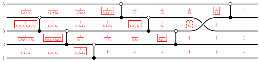
(a) open Richardson variety (Example 6.28)

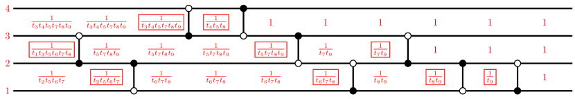
(b) double Bruhat cell (Example 6.30)

Figure 28. Comparing grid minors to chamber minors of [Ing19, FZ99].

Example 6.28.

Consider the running example of [Ing19]: $w=s_{3}s_{2}s_{1}s_{4}s_{3}s_{2}s_{3}s_{4}$ and $u=s_{3}$, which was already considered in the introduction (Figure 4). Applying the parametrization (6.12) and computing $(X_{\bullet},Y_{\bullet})$ from it using the above algorithm, we arrive at the following sequence of matrices $Z_{c}=Y_{c}^{-1}X_{c}$:

$$\text{\scalebox{0.768}{$Z_{0}=\left[\begin{smallmatrix}0&0&0&0&t_{4}t_{5}t_{6}\\ 0&0&0&-t_{1}t_{2}t_{3}&0\\ 0&0&\frac{t_{8}}{t_{1}t_{4}}&0&0\\ 0&-\frac{1}{t_{2}t_{5}}&0&0&0\\ \frac{1}{t_{3}t_{6}t_{8}}&0&0&0&0\end{smallmatrix}\right]$,}}\quad\text{\scalebox{0.768}{$Z_{1}=\left[\begin{smallmatrix}0&0&0&0&t_{4}t_{5}t_{6}\\ 0&0&t_{1}t_{2}t_{3}&-\frac{t_{8}}{t_{4}}&0\\ 0&0&t_{2}t_{3}&0&0\\ 0&-\frac{1}{t_{2}t_{5}}&0&0&0\\ \frac{1}{t_{3}t_{6}t_{8}}&0&0&0&0\end{smallmatrix}\right]$,}}\quad\dots,\quad\text{\scalebox{0.768}{$Z_{8}=\left[\begin{smallmatrix}0&-t_{4}t_{5}t_{6}&t_{4}&t_{4}t_{5}-t_{8}&1\\ t_{1}t_{2}t_{3}&-t_{1}t_{2}-t_{1}t_{6}-t_{5}t_{6}&1&t_{1}+t_{5}&0\\ t_{2}t_{3}&-t_{2}-t_{6}&0&1&0\\ t_{3}&-1&0&0&0\\ 1&0&0&0&0\end{smallmatrix}\right]$.}}$$

The associated grid minors are computed in Figure 28(a). Applying the monomial transformation in [GL22b, Example 11.7], we see that these minors coincide with the ones given in [Ing19, Figure 7.8].

6.6.2. Double Bruhat cells

For $w,v\in S_{n}$, consider the double Bruhat cell $G^{w,v}$ and the reduced double Bruhat cell $L^{w,v}$ defined by

$$G^{w,v}:=B_{+}wB_{+}\cap B_{-}vB_{-}\quad\text{and}\quad L^{w,v}:=G^{w,v}/H.$$

Let $\beta=(i_{1},i_{2},\dots,i_{m})$, where $m=\ell(w)+\ell(v)$, be a double reduced word for $(w,v)$; that is, it is a shuffle of a reduced word for $w$ on positive indices and a reduced word for $v$ on negative indices. The following map is an isomorphism by an argument similar to [WY07, Proposition 2.1]:

(6.13) $$L^{w,v}\xrightarrow{\sim}\accentset{\circ}{R}_{{\operatorname{id}},\beta},\quad g\mapsto(X_{\bullet},Y_{\bullet}),$$

where $(X_{\bullet},Y_{\bullet})$ satisfies the following conditions:

$$\pi(X_{0})=B_{+},\quad X_{m}=g^{-\iota}U_{+},\quad\pi(Y_{0})=B_{-},\quad\text{and}\quad Y_{m}=g^{-\iota}\dot{w}_{0}^{-1}U_{+}.$$

Applying the relations (6.10), we compute $X_{m-1},\dots,X_{0}$ and $Y_{m-1},\dots,Y_{0}$ iteratively. In order to compare our minors to the minors considered in [FZ99, BFZ05], let us choose a parametrization

$$g:=g_{1}\cdots g_{m},\qquad\text{where}\qquad g_{c}=\begin{cases}y_{i_{c}}(t_{c})&\mbox{if $i_{c}>0$,}\\ x_{|i_{c}|}(t_{c})&\mbox{if $i_{c}<0$.}\end{cases}$$

The nonzero parameters $t_{1},\dots,t_{m}$ are expressed as monomials in the cluster variables of [FZ99, BFZ05] computed on the twisted matrix $\xi^{w,v}(g)$; see [FZ99, Definition 1.5]. Given a matrix $x\in B_{-}B_{+}$, let us denote by $([x]_{-},[x]_{0},[x]_{+})\in U_{-}\times H\times U_{+}$ its LDU factorization. One can check that for any $g\in G^{w,v}$, the matrix $g_{0}:=[\dot{w}^{-1}g]_{0}$ is well defined.

It follows from the definition of the map (6.13) that we have $Z_{c}\in H\dot{w}_{0}$ for each $c\in[0,m]$. In particular, the red and the blue grid minors coincide: $\Delta_{c,h}=\Delta_{c,-h}$ for all $c,h$. We leave the verification of the following result to an interested reader.

Proposition 6.29.

Under the isomorphism (6.13), the grid minors $\Delta_{c,h}$ are equal to the chamber minors of [FZ99, Section 4.5] evaluated at $g_{0}\xi^{w,v}(g)$. In particular, all chamber and grid minors from Definitions 6.18 and 6.21 take positive values on the image of the totally positive part $G_{>0}^{w,v}\subset G^{w,v}$ under (6.13).

Example 6.30.

We consider the running example of [FZ99, Section 4.5], except that we ignore the $H$-part factors in their decomposition (marked by green points in [FZ99, Figure 4]). Thus, we have

$$\beta=(2,-1,3,-3,-2,1,2,-1,1),\quad w=s_{2}s_{3}s_{1}s_{2}s_{1},\quad v=s_{1}s_{3}s_{2}s_{1},\quad u={\operatorname{id}}.$$

The matrices $g$, $g_{0}$, and $g_{0}\xi^{w,v}(g)$ are given by

$$g=\left[\begin{smallmatrix}t_{2}t_{5}t_{7}t_{9}+t_{2}t_{6}t_{8}t_{9}+t_{2}t_{6}+t_{2}t_{9}+t_{8}t_{9}+1&t_{2}t_{5}t_{7}+t_{2}t_{6}t_{8}+t_{2}+t_{8}&t_{2}t_{5}&0\\ t_{5}t_{7}t_{9}+t_{6}t_{8}t_{9}+t_{6}+t_{9}&t_{5}t_{7}+t_{6}t_{8}+1&t_{5}&0\\ t_{1}t_{5}t_{7}t_{9}+t_{1}t_{6}t_{8}t_{9}+t_{1}t_{6}+t_{1}t_{9}+t_{7}t_{9}&t_{1}t_{5}t_{7}+t_{1}t_{6}t_{8}+t_{1}+t_{7}&t_{1}t_{5}+1&t_{4}\\ t_{3}t_{7}t_{9}&t_{3}t_{7}&t_{3}&t_{3}t_{4}+1\end{smallmatrix}\right] g_{0}=\left[\begin{smallmatrix}t_{3}t_{7}t_{9}&0&0&0\\ 0&\frac{t_{1}t_{6}}{t_{9}}&0&0\\ 0&0&\frac{1}{t_{6}t_{7}}&0\\ 0&0&0&\frac{1}{t_{1}t_{3}}\end{smallmatrix}\right]$$, , and

$$g_{0}\xi^{w,v}(g)=\left[\begin{smallmatrix}\frac{t_{2}t_{5}t_{7}t_{9}+t_{2}t_{6}t_{8}t_{9}+t_{2}t_{6}+t_{2}t_{9}+t_{8}t_{9}+1}{t_{2}t_{5}}&\frac{t_{8}t_{9}+1}{t_{8}}&\frac{1}{t_{4}t_{5}t_{8}}&1\\ \frac{t_{2}t_{6}+1}{t_{2}t_{5}t_{9}}&\frac{1}{t_{8}t_{9}}&\frac{1}{t_{4}t_{5}t_{8}t_{9}}&\frac{1}{t_{9}}\\ \frac{1}{t_{2}t_{5}t_{6}t_{7}}&\frac{1}{t_{6}t_{7}t_{8}}&\frac{t_{6}t_{8}+1}{t_{4}t_{5}t_{6}t_{7}t_{8}}&\frac{t_{6}t_{8}+1}{t_{6}t_{7}}\\ 0&\frac{t_{2}}{t_{1}t_{3}t_{8}}&\frac{t_{1}t_{5}t_{8}+t_{2}t_{6}t_{8}+t_{2}+t_{8}}{t_{1}t_{3}t_{4}t_{5}t_{8}}&\frac{t_{1}t_{3}t_{4}t_{5}t_{8}+t_{1}t_{5}t_{8}+t_{2}t_{6}t_{8}+t_{2}+t_{8}}{t_{1}t_{3}}\end{smallmatrix}\right]$$.

One can check that the chamber minors from [FZ99, Figure 6] computed on the matrix $g_{0}\xi^{w,v}(g)$ coincide with the red grid minors computed in Figure 28(b).

Remark 6.31.

The chamber minors of [FZ99] computed on the matrix $\xi^{w,v}(g)$ have a description in terms of strands in a double wiring diagram; see [FZ99, Theorem 4.11]. If one computes them on the matrix $g_{0}\xi^{w,v}(g)$ instead, one gets a similar description: each chamber minor equals $\left(\prod t_{k}\right)^{-1}$, where the product is taken over all crossings which are to the right of the chamber and such that the chamber is located vertically between the two strands participating in the crossing. In other words, the transformation $\xi^{w,v}(g)\mapsto g_{0}\xi^{w,v}(g)$ gauge-fixes to $1$ the chamber minors corresponding to the chambers open on the right.

7. Deodhar geometry and seeds

Let $u\leq\beta$. We will use the $u$-positive distinguished subexpression (cf. Section 3.1) to define a torus in $\accentset{\circ}{R}_{{u,\beta}}$, which will ultimately be a cluster torus. We will then use $(u,d)$-almost positive sequences (cf. Section 3.6) to define hypersurfaces in $\accentset{\circ}{R}_{{u,\beta}}$, and in turn to define cluster variables for $\accentset{\circ}{R}_{{u,\beta}}$.

7.1. The Deodhar torus

We continue to denote the $u$-PDS by ${\mathbf{u}}=(u_{(0)},\dots,u_{(m)})$.

Definition 7.1.

The Deodhar torus $T_{{u,\beta}}\subset\accentset{\circ}{R}_{{u,\beta}}$ is the subset of $\accentset{\circ}{R}_{{u,\beta}}$ given by the conditions

(7.1) $$X_{c}\stackrel{{\scriptstyle w_{0}u_{(c)}}}{{\Longleftarrow}}Y_{c}\qquad\mbox{ for $c=0,1,\ldots,m$.}$$

Remark 7.2.

Points in $T_{{u,\beta}}$ lift to walks of the sort described in Remark 6.7 where at each step, one greedily increases the relative position of $X_{c}$ and $Y_{c}$.

Recall from the proof of Lemma 6.19 that all grid minors are nonvanishing on the Deodhar torus $T_{{u,\beta}}$.

Lemma 7.3.

1. For each solid $c\in J_{u,\beta}$, the grid minors $(\Delta_{c-1,j})_{j\in\pm I}$ are Laurent monomials in the grid minors $(\Delta_{c,h})_{h\in\pm I}$ and the chamber minor $\Delta_{c}=\Delta_{c-1,i_{c}}$.

2. For each hollow $c\in[m]\setminus J_{u,\beta}$, the grid minors $(\Delta_{c-1,j})_{j\in\pm I}$ are Laurent monomials in the grid minors $(\Delta_{c,h})_{h\in\pm I}$.

3. Every grid minor $\Delta_{c,j}$ is a Laurent monomial in solid chamber minors $(\Delta_{d})_{d\in J_{u,\beta}}$.

Démonstration.

It suffices to verify the statement on $T_{{u,\beta}}$.

(1) and (2): Set $i:=i_{c}$. We assume $c$ is red, as the other case is similar. By Lemma 6.20, we only need to check the statement for blue grid minors and, if $c$ is hollow, additionally for $\Delta_{c-1,i}$. (For $c$ solid, the statement is vacuously true for $\Delta_{c-1,i}=\Delta_{c}$.) Consider a point $(X_{\bullet},Y_{\bullet})\in T_{{u,\beta}}$. Following the proof of Lemma 6.19, let us choose representative matrices $X_{c},Y_{c}$ such that $Z_{c}=h(w_{0}u_{(c)})^{\mathchoice{\mathbin{\vbox{\hbox{\scalebox{0.4}{$\displaystyle\bullet$}}}}}{\mathbin{\vbox{\hbox{\scalebox{0.4}{$\textstyle\bullet$}}}}}{\mathbin{\vbox{\hbox{\scalebox{0.4}{$\scriptstyle\bullet$}}}}}{\mathbin{\vbox{\hbox{\scalebox{0.4}{$\scriptscriptstyle\bullet$}}}}}}$ for some $h\in H$. With this choice (cf. Remark 6.4), we find that for some $t\in{\mathbb{C}}$,

Set $Z:=Z_{c}$, so $Z_{c-1}=Zz_{i}(t)$. We use the following elementary calculation to compare grid minors at $c-1$ to those at $c$.

(7.2) $$\Delta_{A,B}(Zz_{i}(t))=\begin{cases}\Delta_{A,B}(Z)&\text{ if }s_{i}(B)=B,\\ -\Delta_{A,s_{i}(B)}(Z)&\text{ if }s_{i}(B)<B,\\ t\Delta_{A,B}(Z)+\Delta_{A,s_{i}(B)}(Z)&\text{ if }s_{i}(B)>B.\\ \end{cases}$$

Recall that $Z=h(w_{0}u_{(c)})^{\mathchoice{\mathbin{\vbox{\hbox{\scalebox{0.4}{$\displaystyle\bullet$}}}}}{\mathbin{\vbox{\hbox{\scalebox{0.4}{$\textstyle\bullet$}}}}}{\mathbin{\vbox{\hbox{\scalebox{0.4}{$\scriptstyle\bullet$}}}}}{\mathbin{\vbox{\hbox{\scalebox{0.4}{$\scriptscriptstyle\bullet$}}}}}}$, so many minors of $Z$ vanish. If the crossing $c$ is hollow (so $u_{(c-1)}<u_{(c)}$), then when in the third case of (7.2), the minor multiplying $t$ is always zero. This is enough to show the blue grid minor $\Delta_{c-1,j}$ equals $\Delta_{c,j}$. One can check further that

$$\Delta_{c-1,i}=\frac{\Delta_{c,i-1}\Delta_{c,i+1}}{\Delta_{c,i}}.$$

If $c$ is solid, then (7.2) implies $t=\Delta_{c}/\Delta_{c,i}$, and that a blue grid minor $\Delta_{c-1,j}$ is either equal to $\Delta_{c,j}$ or it is equal to $t\Delta_{c,j}$. Both of these are Laurent monomials in the desired set of grid minors.

(3): Gauge-fix so that $Y_{m}=U_{+}$ and $X_{m}=(w_{0}u)^{\mathchoice{\mathbin{\vbox{\hbox{\scalebox{0.4}{$\displaystyle\bullet$}}}}}{\mathbin{\vbox{\hbox{\scalebox{0.4}{$\textstyle\bullet$}}}}}{\mathbin{\vbox{\hbox{\scalebox{0.4}{$\scriptstyle\bullet$}}}}}{\mathbin{\vbox{\hbox{\scalebox{0.4}{$\scriptscriptstyle\bullet$}}}}}}U_{+}$. All of the grid minors $\Delta_{m,j}$ are equal to 1, so by (1) and (2), the grid minors $\Delta_{m-1,j}$ are Laurent monomials in the chamber minor $\Delta_{m}$, if $m$ is solid, and are equal to $1$ if $m$ is hollow. Continuing from right to left, (1) implies that all grid minors $\Delta_{c,j}$ are Laurent monomials in the solid chamber minors $\{\Delta_{d}\}_{d\in J_{u,\beta}\mid d\geq c}$. ∎

We now show that the Deodhar torus is in fact a torus.

Proposition 7.4.

1. The Deodhar torus $T_{{u,\beta}}$ is an open subset of $\accentset{\circ}{R}_{{u,\beta}}$, isomorphic to an algebraic torus of dimension $d({u,\beta})$.

2. The character lattice of $T_{{u,\beta}}$ consists of Laurent monomials in the solid chamber minors $\Delta_{c}$, $c\in J_{u,\beta}$. The ring of regular functions on $T_{{u,\beta}}$ is the ring of Laurent polynomials in the chamber minors.

3. The grid minors are characters of $T_{{u,\beta}}$.

Démonstration.

We will show that the map $T_{{u,\beta}}\to({{\mathbb{C}}^{\times}})^{d({u,\beta})}$ sending a point to the tuple of its solid chamber minors is an isomorphism. This implies all three of the claims. Using Lemma 6.14, we assume that $u=w_{0}$. Following 6.13, we set $T_{\beta}:=T_{w_{0},\beta}$ and $d(\beta):=d(w_{0},\beta)=\ell(\beta)-\ell(w_{0})$.

We first show how to uniquely recover a point in $T_{\beta}$ from the nonzero values of $\Delta_{c}$. That is, we show that the map is injective. By Lemma 7.3, it suffices to show that a point in $T_{\beta}$ can be uniquely recovered from its grid minors. Throughout, we gauge-fix $Y_{0}=U_{+}$ and $X_{0}=h\dot{w}_{0}U_{+}$, where $h\in H$.

First, we can recover $X_{0}$ and $Y_{0}$, as $h$ is uniquely determined by the grid minors $\Delta_{0,j}$.

Now we show for $c\in[m]$ that if $X_{c-1},Y_{c-1}$ are known, then $X_{c},Y_{c}$ are uniquely determined by the grid minors. There are two cases, depending on whether $c$ is solid or hollow.

Case 1: Suppose the crossing $c$ is solid, so $u_{(c-1)}=u_{(c)}$. Let $i:=i_{c}$. If $c$ is red, resp., blue, we have

    resp.,    

for a unique $t\in{{\mathbb{C}}^{\times}}$. So $Z_{c}=Z_{c-1}z_{i}(t)^{-1}$ if $c$ is red, and $Z_{c}=\bar{z}_{|i|^{*}}(t)Z_{c-1}$ if $c$ is blue. We would like to find $t$. By a formula analogous to (7.2), we have $t=\Delta_{c,i}/\Delta_{c-1,i}$. So $X_{c},Y_{c}$ can be recovered from the grid minors and thus from the chamber minors.

Case 2: Suppose the crossing $c$ is hollow, so $u_{(c-1)}<u_{(c)}$. In this case, $X_{c-1}$ and $Y_{c-1}$ satisfy the conditions of Lemma 6.6(1) if $c$ is red and Lemma 6.6(2) if $c$ is blue. So $X_{c}$ and $Y_{c}$ are uniquely determined.

To show $T_{\beta}\to({{\mathbb{C}}^{\times}})^{d(\beta)}$ is also surjective, we must check that an arbitrary tuple in $({{\mathbb{C}}^{\times}})^{d(\beta)}$ is the list of chamber minors for a point of $T_{\beta}$. To see this, we define a point of $T_{\beta}$ moving right to left. Set $Y_{m}=X_{m}=U_{+}$. Then, supposing we have defined $X_{c}=gU_{+}$ and $Y_{c}=fU_{+}$, let $t:=\Delta_{c-1,i_{c}}/\Delta_{c,i_{c}}$ and define

$$X_{c-1}=\begin{cases}gz_{i_{c}}(t)U_{+}&\text{ if }i_{c}>0,\\ X_{c}&\text{ if }i_{c}<0,\end{cases}\quad\text{and}\quad Y_{c-1}=\begin{cases}Y_{c}&\text{ if }i_{c}>0,\\ f\bar{z}_{{i_{c}}^{*}}(t)U_{+}&\text{ if }i_{c}<0.\end{cases}$$

This produces a point in $T_{\beta}$ by Lemma 6.5. Using (7.2) or similar formulas, one can also check that its chamber minors are equal to the desired tuple. ∎

While the braid variety $\accentset{\circ}{R}_{{u,\beta}}$ is unchanged by braid moves, the Deodhar torus $T_{{u,\beta}}$ may change. In particular, we will show later that non-mutation moves and color-changing moves preserve the Deodhar torus, while mutation moves change it.

7.2. Deodhar hypersurfaces

For $d\in J_{u,\beta}$, recall the notion of the $(u,d)$-almost positive sequence $(v_{(0)}^{{\langle}d{\rangle}},\dots,v_{(0)}^{{\langle}m{\rangle}})$ from Definition 3.15. In this section, we use the $(u,d)$-APS for solid $d$ to define Deodhar hypersurfaces for $\accentset{\circ}{R}_{{u,\beta}}$.

Definition 7.5.

Let $d\in J_{u,\beta}^{\operatorname{mut}}$. Define the mutable Deodhar hypersurface $V_{d}\subset\accentset{\circ}{R}_{{u,\beta}}$ to be the closure of the locus satisfying

(7.3) $$X_{c}\stackrel{{\scriptstyle w_{0}v_{(c)}^{{\langle}d{\rangle}}}}{{\Longleftarrow}}Y_{c}\quad\text{for all $c\in[0,m]$.}$$

Abusing notation, also denote $V_{d}\subset\accentset{\circ}{\mathcal{Y}}_{{u,\beta}}\subset\mathcal{Y}_{{u,\beta}}$.

Remark 7.6.

Points in the locus satisfying (7.3) lift to walks of the sort described in Remark 6.7 where at every step besides step $d$, one greedily increases the relative position of $X_{c}$ and $Y_{c}$. At step $d$, one makes a “mistake” and decreases the relative position of $X_{d}$ and $Y_{d}$.

Proposition 7.7.

The closed subset $\accentset{\circ}{R}_{{u,\beta}}\setminus T_{{u,\beta}}$ is the union of the mutable Deodhar hypersurfaces $V_{d}$ for $d\in J_{u,\beta}^{\operatorname{mut}}$. Each Deodhar hypersurface $V_{d}$ is irreducible and has codimension $1$ in $\accentset{\circ}{R}_{{u,\beta}}$.

Démonstration.

Parametrizing $\mathcal{Y}_{{u,\beta}}$ using (6.4), the conditions (7.3) cut out an iterated fiber bundle over $G/U_{+}\times G/U_{+}$, where each fiber is either ${\mathbb{C}}$, ${{\mathbb{C}}^{\times}}$, or (in the case of the crossing $c=d$) a point. This is an irreducible variety that is codimension one in $\mathcal{Y}_{{u,\beta}}$. The condition that $d\in J_{u,\beta}^{\operatorname{mut}}$ implies that this locus belongs to $\accentset{\circ}{\mathcal{Y}}_{{u,\beta}}$, and in particular, that the action of $G$ is free. It follows that $V_{d}\subset\accentset{\circ}{R}_{{u,\beta}}$ is a codimension $1$ irreducible hypersurface.

Let $(X_{\bullet},Y_{\bullet})\in\accentset{\circ}{R}_{{u,\beta}}\setminus T_{{u,\beta}}$ belong to the complement. Then one of the conditions (7.1) fails. Let $d\in[0,m]$ be equal to the largest value of $c$ for which (7.1) fails. Let $V^{\prime}_{d}\subset\accentset{\circ}{R}_{{u,\beta}}$ be the locus of points where (7.1) holds for $c>d$ and fails for $c=d$. By Lemma 6.5 and the definition of the almost positive subexpression $(v_{(0)}^{{\langle}d{\rangle}},\dots,v_{(0)}^{{\langle}m{\rangle}})$, an open dense subset $V^{\prime\prime}_{d}$ of $V^{\prime}_{d}$ satisfies (7.3). Recall that when $d\in J_{u,\beta}$ is a frozen crossing, the $0$-th term $v_{(0)}^{{\langle}d{\rangle}}$ of the $(u,d)$-APS is not equal to the identity. Thus, if $d\notin J_{u,\beta}^{\operatorname{mut}}$ then $V^{\prime\prime}_{d}$, and therefore $V^{\prime}_{d}$ itself, is empty, a contradiction. Thus, $d\in J_{u,\beta}^{\operatorname{mut}}$ and $(X_{\bullet},Y_{\bullet})$ belongs to the hypersurface $V_{d}$. ∎

When $d\in J_{u,\beta}^{\operatorname{fro}}$, elements $(X_{\bullet},Y_{\bullet})$ satisfying (7.3) do not lie in $\accentset{\circ}{R}_{{u,\beta}}$. In this case, we must define the corresponding Deodhar hypersurface inside $\mathcal{Y}_{{u,\beta}}$.

Definition 7.8.

Let $d\in J_{u,\beta}^{\operatorname{fro}}$. Define the frozen Deodhar hypersurface $V_{d}\subset\mathcal{Y}_{{u,\beta}}$ as the closure of the locus satisfying (7.3).

The following result follows from the same argument as in the proof of Proposition 7.7.

Lemma 7.9.

For $d\in J_{u,\beta}^{\operatorname{fro}}$, the subvariety $V_{d}\subset\mathcal{Y}_{{u,\beta}}$ is irreducible and codimension $1$ in $\mathcal{Y}_{{u,\beta}}$.

Let ${\mathrm{ord}}_{V}f\in{\mathbb{Z}}$ denote the order of vanishing of a rational function $f$ on a hypersurface $V$. Note that if $f\in{\mathbb{C}}(\accentset{\circ}{R}_{{u,\beta}})$ we can calculate ${\mathrm{ord}}_{V}f$ in $\accentset{\circ}{R}_{{u,\beta}}$ or pull it back to $\accentset{\circ}{\mathcal{Y}}_{{u,\beta}}$ and calculate ${\mathrm{ord}}_{V}f$ there. In the case that $V$ is a frozen Deodhar hypersurface, we compute ${\mathrm{ord}}_{V}f$ by pulling $f$ back to $\accentset{\circ}{\mathcal{Y}}_{{u,\beta}}$ and then viewing $f$ as a rational function on $\mathcal{Y}_{{u,\beta}}$. When $f$ is a grid minor, its pullback to $\accentset{\circ}{\mathcal{Y}}_{u,\beta}$ and extension to $\mathcal{Y}_{u,\beta}$ are regular functions in view of Lemma 6.19.

Proposition 7.10.

Fix $d\in J_{u,\beta}$. For $j\in I$,

$${\mathrm{ord}}_{V_{d}}\Delta_{c,j}=\begin{cases}1&\text{ if }u_{(c)}[j]\neq v_{(c)}^{{\langle}d{\rangle}}[j],\\ 0&\text{ otherwise,}\end{cases}\quad\text{and}\quad{\mathrm{ord}}_{V_{d}}\Delta_{c,-j}=\begin{cases}1&\text{ if }u^{-1}_{(c)}[j]\neq(v_{(c)}^{{\langle}d{\rangle}})^{-1}[j],\\ 0&\text{ otherwise.}\end{cases}$$

Démonstration.

We compute the order of vanishing inside the space $S\subset\mathcal{Y}_{u,\beta}$ of tuples $(X_{\bullet},Y_{\bullet})$ of the form (6.5) (i.e., the space where $X_{0}$ has been gauge-fixed to $U_{+}$). This space $S$ is an affine space with coordinates ${\mathbf{t}}=(t_{1},t_{2},\ldots)$, as each $X_{i}$ or $Y_{i}$ is of the form $z_{i_{j_{1}}}(t_{j_{1}})\cdots z_{i_{j_{r}}}(t_{j_{r}})$ or $\bar{z}_{i_{j_{1}}}(t_{j_{1}})\cdots\bar{z}_{i_{j_{r}}}(t_{j_{r}})$ for some $r$. (These coordinates differ from those given by (6.4).) The $Z_{c}$ are then also products of inverses of braid matrices in some subset of the parameters ${\mathbf{t}}$.

Let $Z$ be any matrix that is a product of braid matrices or their inverses with parameters from ${\mathbf{t}}$, each parameter used at most once. Then it is easy to see that every minor of $Z$ is linear or constant in each variable $t_{i}$. The Deodhar hypersurface $V_{d}$ is cut out by a minor of $Z_{d-1}$, and this minor has degree one in some parameter $t=t_{i(d)}$. Any grid minor $\Delta_{c,j}$ is at most degree one in $t$, and thus vanishes to order at most one on $V_{d}$.

Suppose $j\in I$. Then $u_{(c)}[j]=v_{(c)}^{{\langle}d{\rangle}}[j]$ if and only if for a generic point in $V_{d}$, the $j$-th subspace in the weighted flag $X_{c}$ has the correct relative position (given by $u_{(c)}[j]$) with respect to $Y_{c}$. This holds if and only if $\Delta_{c,j}$ does not vanish on $V_{d}$. As we showed above, ${\mathrm{ord}}_{V_{d}}\Delta_{c,j}\leq 1$, and thus we obtain the stated formula for $j\in I$. The argument for $j\in-I$ is identical. ∎

Proposition 7.11.

The map

(7.4) $$f\mapsto({\mathrm{ord}}_{V_{c}}f)_{c\in J_{u,\beta}}$$

is an isomorphism from the character lattice of $T_{{u,\beta}}$ to ${\mathbb{Z}}^{d({u,\beta})}$.

Démonstration.

Let $C\subset{\mathbb{Z}}^{d({u,\beta})}$ be the image of $\{\Delta_{c}\}_{c\in J_{u,\beta}}$. By Proposition 7.10, the chamber minor $\Delta_{c}$ vanishes to order $1$ on $V_{c}$, and does not vanish on $V_{d}$ for $d<c$. Thus, there is an upper unitriangular matrix taking the standard basis of ${\mathbb{Z}}^{d({u,\beta})}$ to $C$. In particular, the images of the chamber minors form a basis of ${\mathbb{Z}}^{d({u,\beta})}$. ∎

7.3. Seeds

The isomorphism (7.4) allows us to define new distinguished characters on $T_{{u,\beta}}$, which will be the cluster variables.

Definition 7.12.

For $c\in J_{u,\beta}$, we define the cluster variable $x_{c}$ to be the unique character of $T_{{u,\beta}}$ that vanishes to order one on $V_{c}$ and has neither a pole nor a zero on $V_{c^{\prime}}$ for $c^{\prime}\in J_{u,\beta}\setminus\{c\}$. We denote the cluster by ${\mathbf{x}}_{u,\beta}=\{x_{c}\}_{c\in J_{u,\beta}}$.

Example 7.13.

Continuing Example 6.24, we see that in the notation of Figure 27, the cluster variables are given by

$$x_{1}=t_{1}t_{4}+1,\quad x_{2}=t_{2}t_{4}t_{5}-1,\quad x_{4}=t_{4},\quad x_{5}=t_{5}.$$

In particular, $\Delta_{4}=t_{4}t_{5}=x_{4}x_{5}$ factors as a product of two cluster variables.

It is immediate from the definition that each cluster variable is a regular function on $\accentset{\circ}{R}_{{u,\beta}}$ and in particular each frozen variable is a unit in ${\mathbb{C}}[\accentset{\circ}{R}_{u,\beta}]$. It is also immediate that the cluster variables in ${\mathbf{x}}_{u,\beta}$ are algebraically independent and irreducible.

Recall the definition of the ice quiver $\widetilde{Q}_{u,\beta}$ from (3.3). The vertices of $\widetilde{Q}_{u,\beta}$ are labeled by $c\in J_{u,\beta}$, as are the elements of ${\mathbf{x}}_{u,\beta}$. So we define the seed

(7.5) $$\Sigma_{u,\beta}:=({\mathbf{x}}_{u,\beta},\widetilde{Q}_{u,\beta}).$$

We may now state our main result.

Theorem 7.14.

For all $u\leq\beta$, we have

$${\mathbb{C}}[\accentset{\circ}{R}_{u,\beta}]=\mathcal{A}(\Sigma_{u,\beta})$$

as subrings of ${\mathbb{C}}(\accentset{\circ}{R}_{{u,\beta}})$. Moreover, the cluster algebra $\mathcal{A}(\Sigma_{u,\beta})$ is locally acyclic and really full rank.

The proof of the isomorphism will occupy Sections 8–9. The local acyclicity and the really full rank property of $\mathcal{A}(\Sigma_{u,\beta})$ are Corollaries 5.8 and 5.9.

We say that a cluster variable $x_{c}$ appears in a grid minor $\Delta_{d,h}$ if ${\mathrm{ord}}_{V_{c}}\Delta_{d,h}=1$. One characterization for when this happens is given by Proposition 7.10. We now relate it to the combinatorics of 3D plabic graphs; cf. Section 2.4. Recall from Section 3.4 that for each $d\in J_{u,\beta}$ we have a relative cycle $C_{d}$ in $G_{u,\beta}$ which bounds a disk $D_{d}$. Recall also from Remark 6.22 that we decorate the faces of the projections of $G_{u,\beta}$ with grid minors.

Lemma 7.15.

Let $d\in J_{u,\beta}$, $c\in[0,m]$, and $h\in I$ (resp., $h\in-I$). Then $x_{d}$ appears in $\Delta_{c,h}$ if and only if $\Delta_{c,h}$ lies in the red (resp., blue) projection of the disk $D_{d}$.

Démonstration.

This follows from Propositions 7.10 and 3.16. Proposition 7.10 computes ${\mathrm{ord}}_{V_{d}}\Delta_{c,h}$ by comparing certain subsets: $u_{(c)}[h]$ and $v_{(c)}^{{\langle}d{\rangle}}[h]$ for the red minor, and $(u_{(c)})^{-1}[|h|]$ and $(v_{(c)}^{{\langle}d{\rangle}})^{-1}[|h|]$ for the blue minor.

Proposition 3.16 shows that the permutation $v_{(c)}^{{\langle}d{\rangle}}$ can be recovered from the monotone multicurve $\bm{\gamma}^{d,c}$. From the details of this construction, one can conclude that $u_{(c)}[h]\neq v_{(c)}^{{\langle}d{\rangle}}[h]$ if and only if one of the curves in $\bm{\gamma}^{d,c}$ intersects the horizontal line $j=h+0.5$ inside $\Gamma(u_{(c)})$. This is equivalent to the point $(c,h+0.5)$ lying in the red projection of $D_{d}$. Similarly, $(u_{(c)})^{-1}[h]\neq(v_{(c)}^{{\langle}d{\rangle}})^{-1}[h]$ if and only if one of the curves in $\bm{\gamma}^{d,c}$ intersects the vertical line $i=h+0.5$ in $\Gamma(u_{(c)})$ if and only if $(c,h+0.5)$ lies in the blue projection of $D_{d}$. Comparing with Proposition 7.10 gives the result. ∎

Example 7.16.

Recall from Example 7.13 that in Figure 27, we have $\Delta_{4}=x_{4}x_{5}$. This is consistent with the fact that the face of $\pi_{\operatorname{red}}(G_{u,\beta})$ containing $\Delta_{4}=\Delta_{3,1}$ lies inside the cycles $C_{4},C_{5}$ shown in Figure 6(e).

We now give an alternate construction of $\widetilde{Q}_{u,\beta}$ related to the half-arrow description in Section 3.7. First, consider a collection $P_{{u,\beta}}^{+}$ (resp., $P_{{u,\beta}}^{-}$) of half-arrows between the red (resp., blue) grid minors $\{\Delta_{c,h}\}_{c\in[0,m],h\in I}$ (resp., $\{\Delta_{c,h}\}_{c\in[0,m],h\in-I}$). It is obtained by placing the following configuration of half-arrows around each bridge $b_{c}$ with $i_{c}>0$ in $\pi_{\operatorname{red}}(G_{u,\beta})$ (resp., each blue bridge $b_{c}$ with $i_{c}<0$ in $\pi_{\operatorname{blue}}(G_{u,\beta})$), where $i:=|i_{c}|$:

Proposition 7.17.

Define a quiver with vertex set ${\mathbf{x}}_{u,\beta}$ as follows. Write each grid minor as

$$\Delta_{d,h}=\prod_{c\in J_{u,\beta}}x_{c}^{q^{c}_{d,h}},$$

where $q^{c}_{d,h}:={\mathrm{ord}}_{V_{c}}\Delta_{d,h}\geq 0$. For every half-arrow $\Delta_{d,h}\to\Delta_{d^{\prime},h^{\prime}}$ in $P_{{u,\beta}}^{+}$ and $P_{{u,\beta}}^{-}$, draw $q^{c}_{d,h}q^{c^{\prime}}_{d^{\prime},h^{\prime}}$ arrows from $x_{c}$ to $x_{c}^{\prime}$. (In other words, for every $x_{c}$ appearing in $\Delta_{d,h}$ and $x_{c}^{\prime}$ appearing in $\Delta_{d^{\prime},h^{\prime}}$, draw a half-arrow $x_{c}\to x_{c}^{\prime}$.) Then delete loops and 2-cycles. The resulting collection of half-arrows agrees with the quiver $\widetilde{Q}_{u,\beta}.$ That is, the signed number of half-arrows between any two vertices is twice the number of arrows between the corresponding vertices of $\widetilde{Q}_{u,\beta}$.

Démonstration.

This follows directly from Lemma 7.15 and Proposition 3.18. ∎

Remark 7.18.

Let $\beta={\mathbf{w}}$ be a reduced word for $w\in S_{n}$. Comparing the above half-arrow description to [Ing19, Definition VII.2] and applying Proposition 6.25, it follows that the isomorphism (6.11) sends Ingermanson’s seed to our seed $\Sigma_{u,\beta}$. Thus, our cluster structure on the open Richardson variety $\accentset{\circ}{R}_{u,w}$ recovers the upper cluster structure on $\accentset{\circ}{R}_{u,w}$ constructed in [Ing19].

8. Moves preserve the cluster algebra

To each $u\leq\beta$, we have associated a seed $\Sigma_{u,\beta}$ and thus also a cluster algebra ${\mathcal{A}}_{{u,\beta}}:={\mathcal{A}}(\Sigma_{u,\beta})\subset{\mathbb{C}}(\accentset{\circ}{R}_{{u,\beta}})$. Our ultimate goal is to show that ${\mathbb{C}}[\accentset{\circ}{R}_{{u,\beta}}]$ is isomorphic to ${\mathcal{A}}_{{u,\beta}}$. As an intermediate step, we show the following.

Theorem 8.1.

Suppose $\beta$ and $\beta^{\prime}$ are related by one of the moves (B1)–(B5). Let $m:\accentset{\circ}{R}_{{u,\beta}}\xrightarrow{\sim}\accentset{\circ}{R}_{{u,\beta^{\prime}}}$ be the corresponding isomorphism from Proposition 6.16. Then the isomorphism $m^{*}:{\mathbb{C}}(\accentset{\circ}{R}_{{u,\beta^{\prime}}})\xrightarrow{\sim}{\mathbb{C}}(\accentset{\circ}{R}_{{u,\beta}})$ restricts to an isomorphism ${\mathcal{A}}_{{u,\beta^{\prime}}}\xrightarrow{\sim}{\mathcal{A}}_{{u,\beta}}$.

Remark 8.2.

If $\beta$ and $\beta^{\prime}$ are related by moves (B1)–(B4), then the quivers $\widetilde{Q}_{u,\beta}$ and $\widetilde{Q}_{u,\beta^{\prime}}$ are related either by relabeling the vertices or by mutation (cf. Theorem 4.3, Proposition 4.7). So in these cases, we have an isomorphism ${\mathcal{A}}_{{u,\beta}}\cong{\mathcal{A}}_{{u,\beta^{\prime}}}$, and to prove Theorem 8.1, we just need to check that the isomorphism is induced by the appropriate isomorphism of braid varieties.

Throughout the following three subsections, we assume that $u=w_{0}$ (cf. 6.13 and 6.14), and that $\beta$ and $\beta^{\prime}$ are related by a single move (B1)–(B5). We let $m:\accentset{\circ}{R}_{\beta}\to\accentset{\circ}{R}_{\beta^{\prime}}$ denote the corresponding isomorphism, defined in Proposition 6.16. Any pullback mentioned is a pullback by $m$. We set $J_{\beta^{\prime}}$ to be the set of solid crossings for $\beta^{\prime}$. For $x_{c}\in{\mathbf{x}}_{\beta^{\prime}}$, we denote $p_{c}:=m^{*}(x_{c})$ and $\mathbf{p}_{\beta^{\prime}}:=\{p_{c}\}_{c\in J_{\beta^{\prime}}}$. The isomorphism $m$ also induces a map on the double cosets $Z_{c}$; we write $Z^{\prime}_{c}$ to denote the image of $Z_{c}$ under this map. Pullbacks of grid minors are also denoted with primes.

8.1. Non-mutation moves and (B4) do not change the seed

In this section, we prove Theorem 8.1 for non-mutation moves and (B4). We show that in this case, $\Sigma_{\beta}$ and $(\mathbf{p}_{\beta^{\prime}},\widetilde{Q}_{\beta^{\prime}})$ differ only by reindexing. As noted in Remark 8.2, it suffices to check this statement for clsuter variables.

Proposition 8.3.

Suppose $\beta$ and $\beta^{\prime}$ are related by a non-mutation move or (B4) and let $\alpha$ be the corresponding relabeling bijection $J_{\beta}\to J_{\beta^{\prime}}$ from Section 4.4. Then $x_{c}=p_{\alpha(c)}$.

Démonstration.

For (B4), $\alpha$ is the identity. It is clear that $\Delta_{c,h}=\Delta_{c,h}^{\prime}$ and $x_{d}$ appears in $\Delta_{c,h}$ if and only if $p_{d}$ appears in $\Delta_{c,h}^{\prime}$. The claim follows. Indeed, suppose $d\in J^{\operatorname{mut}}_{\beta}$ and for all solid $c>d$, we already know $x_{c}=p_{\alpha(c)}$. Then $\Delta_{d-1,i_{d}}=x_{d}M$ and $\Delta_{d-1,i_{d}}^{\prime}=p_{\alpha(d)}M^{\prime}$, where $M$ (resp., $M^{\prime}$) is a product of cluster variables $x_{c}$ (resp, $p_{\alpha(c)}$) with $c>d$. By above, the left-hand sides of these two equations are equal and $M=M^{\prime}$. So e.g. by restricting to the Deodhar torus, we may conclude $x_{d}=p_{\alpha(d)}$.

Now, for non-mutation moves. Suppose the non-mutation move involves the indices in some interval $(l,r]\subset[m]$ of length $2$ or $3$. Let $G^{L}$ (resp., $G^{R}$) denote the portion of $G_{\beta}$ between $\Gamma(u_{(0)})$ and $\Gamma(u_{(l)})$ (resp., between $\Gamma(u_{(r)})$ and $\Gamma(u_{(m)})$). Note that $G^{L}$ (resp., $G^{R}$) is also equal to the portion of $G_{u,\beta^{\prime}}$ between $\Gamma(u^{\prime}_{(0)})$ and $\Gamma(u^{\prime}_{(l)})$ (resp., between $\Gamma(u^{\prime}_{(r)})$ and $\Gamma(u^{\prime}_{(m)})$). By Section 4.4, for all $c\in J_{\beta}$, the cycles $C_{c}$ and $C^{\prime}_{\alpha(c)}$ behave identically on $G^{L}$ and $G^{R}$. This implies a point is contained in the red (resp., blue) projection of $D_{c}$ if and only if it is contained in the red (resp., blue) projection of $D^{\prime}_{\alpha(c)}$. Also, for $c\notin(l,r):=[l+1,r-1]$, we have $\Delta_{c,h}=\Delta_{c,h}^{\prime}$ for all $h\in\pm I$. Using Lemma 7.15, we obtain the following.

Lemma 8.4.

Suppose $c\notin(l,r)$ and $d\in J_{\beta}$. Then $x_{d}$ appears in $\Delta_{c,h}$ if and only if $p_{\alpha(d)}$ appears in $\Delta_{c,h}^{\prime}=\Delta_{c,h}$.

Note that $\alpha$ is the identity on $(r,m]$. The same argument as in the (B4) case shows $x_{c}=p_{\alpha(c)}$ for solid crossings $c>r$. For solid $c\in(l,r]$, to show $x_{c}=p_{\alpha(c)}$, it suffices to find a grid minor $\Delta_{d,h}$ with $d\leq l$ which is a product of $x_{c}$ and other $x_{c^{\prime}}$ which are already known to be equal to $p_{\alpha(c^{\prime})}$. In fact, a grid minor $\Delta_{l,h}$ will always work; this can be seen from Figures 22, 23 and 24 and the rules governing cycles. Now, $\alpha$ is also the identity on $[1,l]$, so the same argument as for (B4) shows $x_{c}=p_{\alpha_{c}}$ for solid $c\leq l$. ∎

8.2. Mutation moves mutate the seed

In this section, we prove Theorem 8.1 for mutation moves. We show that in this case, $\Sigma_{\beta}$ and $(\mathbf{p}_{\beta^{\prime}},\widetilde{Q}_{\beta^{\prime}})$ are related by mutation. This statement has already been checked for the quivers, so we just check the cluster variables.

Lemma 8.5.

Suppose $\beta$ and $\beta^{\prime}$ are related by the mutation move whose rightmost crossing is $c+1$. Then for $d\in J_{\beta}\setminus\{c+1\}$, we have $x_{d}=p_{d}$.

Démonstration.

This argument is similar to the proof of Proposition 8.3. Say the mutation move occurs on indices in the interval $(l,r]\in[m]$, with $r:=c+1$. Then for $h\in[0,l]\cup[r,m]$, the cluster variable $x_{c+1}$ does not appear in grid minors $\Delta_{d,h}$ and $\Delta_{d,h}=\Delta_{d,h}^{\prime}$. Moreover, a cluster variable $x_{c^{\prime}}\neq x_{c+1}$ appears in $\Delta_{d,h}$ for $h\in[0,l]\cup[r,m]$ if and only if $p_{c^{\prime}}$ appears in $\Delta_{d,h}^{\prime}$. The desired equality now follows from a triangularity argument. ∎

Now, we verify that the single new cluster variable in $\mathbf{p}_{\beta^{\prime}}$ satisfies the exchange relation given by $\Sigma_{\beta}$. We will need some identities for grid minors, which we obtain from standard determinantal identities.

The following relations hold on $G$.

Proposition 8.6 (Desnanot–Jacobi identity).

Suppose $p,q\in S_{n}$ and $a\in I$ with $\ell(ps_{a})=\ell(p)+1$ and $\ell(qs_{a})=\ell(q)+1$. Then

(8.1) $$\Delta_{p[a],q[a]}\Delta_{ps_{a}[a],qs_{a}[a]}=\Delta_{ps_{a}[a],q[a]}\Delta_{p[a],qs_{a}[a]}+\Delta_{p[a-1],q[a-1]}\Delta_{p[a+1],q[a+1]}.$$

Proposition 8.7 ([FZ99, Theorem 1.16(1)]).

Let $p,q\in S_{n}$ and $a,b\in I$. Suppose $(s_{a}s_{b})^{3}=1$ and $\ell(qs_{a}s_{b}s_{a})=\ell(q)+3$. Then

(8.2) $$\Delta_{p[a],qs_{a}[a]}\Delta_{p[b],qs_{b}[b]}=\Delta_{p[a],q[a]}\Delta_{p[b],qs_{a}s_{b}[b]}+\Delta_{p[a],qs_{b}s_{a}[a]}\Delta_{p[b],q[b]}.$$

Lemma 8.8.

Let $A,B\subset[n]$ with $|A|=|B|$, $a\in I$, and suppose $s_{a}(A)\geq A$ in the lexicographic order. Then

$$\Delta_{s_{a}(A),B}(\dot{s}_{a}M)=\Delta_{A,B}(M)\quad\text{and}\quad\Delta_{B,s_{a}(A)}(M\dot{s}_{a})=-\Delta_{B,A}(M).$$

Now, we use the determinantal identities above to obtain relations on grid minors before and after a mutation move.

Proposition 8.9.

1. Suppose $\beta,\beta^{\prime}$ are related by a (B1) special solid move $ji\to ij$ on crossings $c,c+1$. Then the grid minors on $\accentset{\circ}{R}_{\beta}$ satisfy

   (8.3) $$\Delta_{c,j}\Delta_{c,j}^{\prime}=\Delta_{c+1,j}\Delta_{c-1,j}+\Delta_{c,j-1}\Delta_{c,j+1}.$$

2. Suppose $\beta,\beta^{\prime}$ are related by a (B3) fully solid move $iji\to jij$ on crossings $c-1,c,c+1$. Then the grid minors on $\accentset{\circ}{R}_{\beta}$ satisfy

   (8.4) $$\Delta_{c,i}\Delta_{c,j}^{\prime}=\Delta_{c+1,i}\Delta_{c-2,j}+\Delta_{c+1,j}\Delta_{c-2,i}.$$

Démonstration.

Set $v:=u_{(c+1)}$.

For (1): We will assume $j<0$ and $i>0$, as the other case is similar. Let $k=-j$. Note that we can write $Z_{c-1},Z_{c}$ and $Z_{c}^{\prime}$ in terms of $Z_{c+1}$:

$$Z_{c-1}=(\bar{z}_{k^{*}}(t^{\prime}))^{-1}Z_{c+1}z_{i}(t)=\dot{s}_{k^{*}}x_{k^{*}}(t^{\prime})Z_{c+1}x_{i}(t)\dot{s}_{i}$$

while $Z_{c}=Z_{c+1}x_{i}(t)\dot{s}_{i}$ and $Z_{c}^{\prime}=\dot{s}_{k^{*}}x_{k^{*}}(t^{\prime})Z_{c+1}$.

Now, apply (8.1) to $Z_{c-1}$ with $p=w_{0}s_{k}$, $q=v^{-1}$, and $a=k$. Using $vs_{i}=s_{k}v>v$, Lemma 8.8, Lemma 6.20, and the $U_{+}\times U_{+}$-invariance of the grid minors, we obtain the equation (8.3). For example,

$$\Delta_{p[a],qs_{a}[a]} =\Delta_{s_{k^{*}}w_{0}[k],s_{i}v^{-1}[k]}(Z_{c-1})=-\Delta_{w_{0}[k],s_{i}v^{-1}[k]}(Z_{c})=\Delta_{w_{0}[k],v^{-1}[k]}(Z_{c+1})=\Delta_{c+1,j}.$$

For (2): Using the same strategy as above, we apply (8.2) to $Z_{c-2}$ (or its transpose) to obtain (8.4). If $i>0$ and $j=i+1$, for example, we set $p=w_{0}v$, $q={\operatorname{id}}$, $a=i$ and $b=i+1$. ∎

We need one additional identity on grid minors to show that $p_{c+1}$ satisfies the correct exchange relation.

Lemma 8.10.

Choose a crossing $c$. Let $a\in[n]$ and let $b=-u_{(c)}(a)$. Then the relation

$$\Delta_{c,a}\Delta_{c,b+1}=\Delta_{c,b}\Delta_{c,a-1}$$

holds on $\accentset{\circ}{R}_{\beta}$, where we set $\Delta_{c,0}=\Delta_{c,\pm n}:=1$.

Démonstration.

It suffices to show that this relation holds on the Deodhar torus $T_{\beta}$, which is dense. As in the proof of Lemma 7.3, we choose representatives $X_{c},Y_{c}$ so that the matrix $Z_{c}$ is of the form

$$g:=Z_{c}=h(w_{0}u_{(c)})^{\mathchoice{\mathbin{\vbox{\hbox{\scalebox{0.4}{$\displaystyle\bullet$}}}}}{\mathbin{\vbox{\hbox{\scalebox{0.4}{$\textstyle\bullet$}}}}}{\mathbin{\vbox{\hbox{\scalebox{0.4}{$\scriptstyle\bullet$}}}}}{\mathbin{\vbox{\hbox{\scalebox{0.4}{$\scriptscriptstyle\bullet$}}}}}}$$

for some $h\in H$. Only the entries $g_{w_{0}u_{(c)}(i),i}$ are nonzero. So for $i>0$, $\Delta_{c,i}$ is (up to sign) the product of the nonzero entries of $g$ in columns $1,\dots,i$. For $i<0$, $\Delta_{c,i}$ is (up to sign) the product of the nonzero entries of $g$ in rows $w_{0}(|i|),w_{0}(|i|)+1,\dots,n$. Using this, we find

$$\frac{\Delta_{c,a}}{\Delta_{c,a-1}}=\frac{\Delta_{c,b}}{\Delta_{c,b+1}}=(-1)^{q}g_{w_{0}(|b|),a}.$$

where $q$ is the number of nonzero entries of $g$ southwest of $g_{w_{0}(|b|),a}$. ∎

Proposition 8.11.

Let $\beta$ and $\beta^{\prime}$ be related by a mutation move whose rightmost crossing is $c+1$. Then $(\mathbf{p}_{\beta^{\prime}},\widetilde{Q}_{\beta^{\prime}})=\mu_{c+1}(\Sigma_{\beta})$.

Démonstration.

Case 1: Suppose the mutation move is a (B1) special solid move $ji\to ij$ on crossings $c,c+1$. Without loss of generality, we may assume $j<0$ and $i>0$. We see from Figure 19(a) and Lemma 7.15 that $x_{c+1}$ appears only in grid minors $\Delta_{c,i}$ and $\Delta_{c,j}$. Using Proposition 7.17, we find that the cluster variable $x^{\prime}_{c+1}$ in $\mu_{c+1}(\Sigma_{\beta})$ satisfies the exchange relation

(8.5) $$x_{c+1}x^{\prime}_{c+1} =(\Delta_{c+1,i}\Delta_{c-1,j}+(\Delta_{c,i-1}\Delta_{c,i+1}\Delta_{c,j-1}\Delta_{c,j+1})^{1/2})/f$$

(8.6) $$=(\Delta_{c+1,i}\Delta_{c-1,j}+\Delta_{c,i-1}\Delta_{c,j-1})/f$$

where $f$ is the cluster monomial

$$f=\prod_{d\neq c+1}x_{d}^{\min({\mathrm{ord}}_{V_{d}}(\Delta_{c+1,i}\Delta_{c-1,j}),{\mathrm{ord}}_{V_{d}}(\Delta_{c,i-1}\Delta_{c,j-1}))}.$$

The equality in (8.6) follows from Lemma 8.10: since $j=-u_{(c)}(i)$ and $j-1=-u_{(c)}(i+1)$, we get $\Delta_{c,j+1}=\Delta_{c,i-1}\Delta_{c,j}/\Delta_{c,i}$ and $\Delta_{c,i+1}=\Delta_{c,j-1}\Delta_{c,i}/\Delta_{c,j}$.

On the other hand, using (8.3) and Lemma 8.10 together, we have that

(8.7) $$\Delta_{c,j}^{\prime}\Delta_{c,i}=\Delta_{c+1,i}\Delta_{c-1,j}+\Delta_{c,i-1}\Delta_{c,j-1}$$

on $\accentset{\circ}{R}_{\beta}$, where $\Delta_{c,j}^{\prime}$ is the grid minor evaluated after the braid move. This can be seen by working on the Deodhar torus and multiplying (8.3) by $\Delta_{c+1,i-1}/\Delta_{c+1,j+1}$; one must also use $\Delta_{c+1,j+1}=\Delta_{c,j+1}$, which follows from the move being special solid.

To show that $p_{c+1}$ obeys the exchange relation, we will prove that the left-hand side of (8.7) is equal to $fx_{c+1}p_{c+1}$. It is easy to check that $x_{c+1}$ appears in $\Delta_{c,i}$ and $p_{c+1}$ appears in $\Delta_{c,j}^{\prime}$. So all that remains is to show that for $d\neq c+1$,

$${\mathrm{ord}}_{V_{d}}(\Delta_{c,j}^{\prime}\Delta_{c,i})=\min({\mathrm{ord}}_{V_{d}}(\Delta_{c+1,i}\Delta_{c-1,j}),{\mathrm{ord}}_{V_{d}}(\Delta_{c,i-1}\Delta_{c,j-1})).$$

Eq. 4.1 implies an analogous statement for (8.3); that is, the order of vanishing of the left-hand side on $V_{d}$ is the minimum of the orders of vanishing of the two terms on the right. Since (8.7) differs from (8.3) by a Laurent monomial in cluster variables, we obtain the desired equality for (8.7).

Case 2: Suppose the mutation move is a (B3) fully solid move $iji\to jij$ on crossings $c-1,c,c+1$. We assume $i>0$; the $i<0$ case is similar. The proof strategy is similar to Case 1, so we will be brief. By Proposition 7.10, the only red grid minors $x_{c+1}$ appears in are $\Delta_{c,i}=\Delta_{c-1,i}$. So by Proposition 7.17, the exchange relation for $x^{\prime}_{c+1}$ is

$$x_{c+1}x^{\prime}_{c+1}=(\Delta_{c+1,i}\Delta_{c-2,j}+\Delta_{c+1,j}\Delta_{c-2,i})/f$$

where $f$ is the cluster monomial

$$f=\prod_{d\neq c+1}x_{d}^{\min({\mathrm{ord}}_{V_{d}}(\Delta_{c+1,i}\Delta_{c-2,j}),{\mathrm{ord}}_{V_{d}}(\Delta_{c+1,j}\Delta_{c-2,i}))}.$$

On the other hand, (8.4) and (4.1) together imply that the right-hand side of the exchange relation is equal to $x_{c+1}p_{c+1}$. ∎

8.3. Move (B5) rescales the seed

In this section, we prove Theorem 8.1 for (B5). If the first crossing is hollow, this is straightforward (Lemma 8.12). If the first crossing is solid, we show that $\Sigma_{\beta}$ and $(\mathbf{p}_{\beta^{\prime}},\widetilde{Q}_{\beta^{\prime}})$ differ only in a single frozen variable and arrows involving that frozen variable, in a way that preserves the cluster algebra (Proposition 8.13).

Lemma 8.12.

Suppose $\beta=(-i)\gamma$ and $\beta^{\prime}=i\gamma$ for some positive double braid $\gamma$. If the first crossing is hollow, then $\Sigma_{\beta}=(\mathbf{p}_{\beta^{\prime}},\widetilde{Q}_{\beta^{\prime}})$.

Démonstration.

Note that the first crossing is hollow in $\beta$ if and only if it is hollow in $\beta^{\prime}$. The color of the hollow crossing does not matter in the definition of the surface $\mathbf{S}_{u,\beta}$ and does not affect the interaction of any mutable cycle with any other cycle, so $\mathbf{S}_{u,\beta}=\mathbf{S}_{u,\beta^{\prime}}$ and $\widetilde{Q}_{\beta}=\widetilde{Q}_{\beta^{\prime}}$. Further, the upper triangular matrix relating chamber minors and cluster variables is the same for both seeds, and all chamber minors pull back to chamber minors. This implies $x_{c}=p_{c}$ for all $c\in J_{\beta}$. ∎

We now assume that the first crossings of $\beta$ and $\beta^{\prime}$ are solid. We would like to apply the following proposition to the two seeds at hand.

Proposition 8.13 ([Fra16], cf. [LS16, Proposition 5.11]).

Suppose $({\mathbf{x}},\widetilde{Q})$ and $({\mathbf{x}}^{\prime},\widetilde{Q}^{\prime})$ are two seeds in $\mathcal{F}$ such that

• $\widetilde{Q}$ and $\widetilde{Q}^{\prime}$ are ice quivers on the same set of vertices, whose mutable parts coincide,

• the mutable variables in ${\mathbf{x}}$ and ${\mathbf{x}}^{\prime}$ are the same, and the two sets of frozen variables are related by an invertible monomial transformation, and

• for each mutable vertex $c$,

  $$\prod_{v\in\widetilde{Q}}x_{v}^{\#\text{arrows }v\to c\text{ in }\widetilde{Q}}=\prod_{v\in\widetilde{Q}^{\prime}}(x_{v}^{\prime})^{\#\text{arrows }v\to c\text{ in }\widetilde{Q}^{\prime}}.$$

Then ${\mathcal{A}}({\mathbf{x}},\widetilde{Q})={\mathcal{A}}({\mathbf{x}}^{\prime},\widetilde{Q}^{\prime})$.

We first analyze the relationship between the clusters ${\mathbf{x}}_{\beta}$ and $\mathbf{p}_{\beta^{\prime}}$.

Lemma 8.14.

Suppose $\beta=(-i)\gamma$ and $\beta^{\prime}=i\gamma$ and the first crossing is solid. Then for $(c,h)\neq(0,\pm i)$, $x_{d}$ appears in $\Delta_{c,h}$ if and only if $p_{d}$ appears in $\Delta_{c,h}$. Further, $x_{c}=p_{c}$ for $c\neq 1$.

Démonstration.

Note that for $(c,h)\neq(0,\pm i)$, $\Delta_{c,h}=\Delta_{c,h}^{\prime}$.

For the first claim: by Proposition 7.10, the appearance of a cluster variable $x_{d}$ in a grid minor $\Delta_{c,h}$ depends only on $d$ and the suffix $i_{c+1}\dots i_{m}$ of $\beta$. The same statement holds for $p_{d}$, $\Delta_{c,h}^{\prime}=\Delta_{c,h}$ and $\beta^{\prime}$. Since for $c>0$, the suffixes of $\beta$ and $\beta^{\prime}$ coincide, this implies the first claim for all grid minors with $c>0$. For $c=0$, by Lemma 6.20, each blue grid minor for $c=0$ besides $\Delta_{0,-|i|}$ is equal to a blue grid minor for $c=1$. It follows from the definition that $\Delta_{0,h}=\Delta_{0,-h}$, so this gives the first claim for grid minors with $(c,h)\neq(0,\pm i)$.

The second claim follows from the first, since cluster variables are unitriangularly related to chamber minors, and the first claim implies the unitriangular matrices for the two seeds differ only in the first row (or column). ∎

Lemma 8.15.

Suppose $\beta=(-i)\gamma$ and $\beta^{\prime}=i\gamma$ and the first crossing is solid. Then $p_{1}=x_{1}^{-1}M$ where $M$ is a Laurent monomial in the frozen variables of ${\mathbf{x}}_{\beta}$ other than $x_{1}$.

Démonstration.

Suppose $i>0$. For $h\in H$, let $h_{j}:=h_{j,j}$.

Gauge-fix as in the proof of Proposition 6.16, so $Z_{0}=h\dot{w}_{0}$ and $Z_{0}^{\prime}=h^{\prime}\dot{w}_{0}$, where $h^{\prime}$ is obtained from $h$ by swapping the positions of $h_{n-i+1}$ and $h_{n-i}$. It is easy to see that $\Delta_{0,a}=\Delta_{0,-a}=h_{n}\cdots h_{n-|a|+1}$, and similarly for $\Delta_{0,a}^{\prime}$. Now, because $x_{1}$ appears in $\Delta_{0,-i}$ but not $\Delta_{0,-(i+1)}$, we have $h_{n-i}=x_{1}^{-1}N$ where $N$ is a Laurent monomial in the other frozen variables of ${\mathbf{x}}_{\beta}$. Similarly, because $p_{1}$ appears in $\Delta_{0,i}^{\prime}$ and not $\Delta_{0,i-1}^{\prime}$, we have $h^{\prime}_{n-i+1}=h_{n-i}=p_{1}N^{\prime}$ where $N^{\prime}$ is a Laurent monomial in the other frozen variables of $\mathbf{p}_{\beta^{\prime}}$. So $p_{1}=x_{1}^{-1}N/N^{\prime}$. Since all frozen variables in $\mathbf{p}_{\beta^{\prime}}\setminus\{p_{1}\}$ are equal to frozen variables of ${\mathbf{x}}_{\beta}$, we have proved the claim. ∎

Lemma 8.16.

Suppose $\beta=(-i)\gamma$ and $\beta^{\prime}=i\gamma$ and the first crossing is solid. For each mutable crossing $c\in J^{\operatorname{mut}}_{\beta}$, we have

(8.8) $$\prod_{d\in\widetilde{Q}_{\beta}}x_{d}^{\#\text{arrows }d\to c\text{ in }\widetilde{Q}_{\beta}}=\prod_{d\in\widetilde{Q}_{\beta^{\prime}}}p_{d}^{\#\text{arrows }d\to c\text{ in }\widetilde{Q}_{\beta^{\prime}}}.$$

Démonstration.

The result follows straighforwardly from Proposition 7.17. Suppose $i>0$. The quiver $P^{+}_{\beta}$ is obtained from $P^{+}_{\beta^{\prime}}$ by adding the half-arrows coming from the leftmost red bridge of $\pi_{\operatorname{red}}(G_{\beta})$; the quiver $P^{-}_{\beta^{\prime}}$ is obtained from $P^{-}_{\beta}$ by adding the half-arrows coming from the leftmost blue bridge of $\pi_{\operatorname{blue}}(G_{u,\beta^{\prime}})$. Together with Lemma 8.14, this implies that the quivers $\widetilde{Q}_{\beta}$ and $\widetilde{Q}_{\beta^{\prime}}$ can be obtained from a third quiver $\widetilde{Q}$ by adding a vertex $x_{1}$ or $p_{1}$ and adding the half-arrows contributed by the leftmost bridge.

As before, for $h\in H$, let $h_{j}:=h_{j,j}$. Gauge-fix as in Proposition 6.16, so $Z_{0}=h\dot{w}_{0}$ and $Z_{0}^{\prime}=h^{\prime}\dot{w}_{0}$, where $h^{\prime}$ is obtained from $h$ by swapping the positions of $h_{n-i+1}$ and $h_{n-i}$.

Fix $c\in J^{\operatorname{mut}}_{\beta}$, and let $L$ and $R$ denote the left- and right-hand sides of (8.8). If $x_{c}$ does not appear in $\Delta_{1,i}$, then there are no arrows between $x_{c}$ and $x_{1}$ and the arrows $x_{d}\to x_{c}$ in $\widetilde{Q}_{\beta}$ are in bijection with arrows $p_{d}\to p_{c}$ in $\widetilde{Q}_{\beta^{\prime}}$. We find that (8.8) follows from Lemma 8.14.

If $x_{c}$ does appear in $\Delta_{1,i}$, then the arrows in $P^{+}_{\beta}$ around the leftmost red bridge contribute

$$\frac{(\Delta_{0,i+1}\Delta_{0,i-1})^{1/2}}{\Delta_{0,i}}=\frac{h_{n-i}^{1/2}}{h_{n-i+1}^{1/2}}$$

to $L$.

From Lemma 8.14, we know $p_{c}$ appears in $\Delta_{1,-i}^{\prime}=\Delta_{1,i}$. The half-arrows in $P^{-}_{\beta^{\prime}}$ around the leftmost blue bridge contribute

$$\frac{\Delta_{0,-i}^{\prime}}{(\Delta_{0,-(i+1)}\Delta_{0,-(i-1)})^{1/2}}=\frac{h_{n-i}^{1/2}}{h_{n-i+1}^{1/2}}$$

to $R$.

Now, if we divide $L$ and $R$ by $(h_{n+i-1}/h_{n-i})^{1/2}$, we obtain two expressions that are equal. Indeed, the expressions are monomials in ${\mathbf{x}}_{\beta}\setminus\{x_{1}\}$ and $\mathbf{p}_{\beta^{\prime}}\setminus\{p_{1}\}$, respectively, and exponents in both expressions are determined by arrows in $\widetilde{Q}$. ∎

9. Proof of Theorem 7.14

In this section, we continue to assume $u=w_{0}$. Recall that to each double braid word $\beta\geq w_{0}$, we have associated a cluster algebra ${\mathcal{A}}_{\beta}\subset{\mathbb{C}}(\accentset{\circ}{R}_{\beta})$. By Theorem 8.1, this cluster algebra is invariant under (B1)–(B5). We prove that ${\mathbb{C}}[\accentset{\circ}{R}_{\beta}]$ is equal to ${\mathcal{A}}_{\beta}$ by induction on the length $\ell=\ell(\beta)$.

9.1. Reduction to $ii\beta^{\prime}$

Using Theorem 8.1 and arguing as in the beginning of Theorem 5.6, we may assume $\beta=ii\beta^{\prime}$ is a double braid in positive letters starting with $ii$. Note that the index $1\in J_{\beta}$ is solid and the cluster variable $x_{1}$ is frozen.

We first deal with the case that the second $i$ is hollow, i.e., $2\notin J_{\beta}$.

Proposition 9.1.

If $2\notin J_{\beta}$, then we have an isomorphism $r:\accentset{\circ}{R}_{\beta}\xrightarrow{\sim}\accentset{\circ}{R}_{i\beta^{\prime}}\times{{\mathbb{C}}^{\times}}$ which induces an isomorphism $r^{*}:{\mathcal{A}}_{i\beta^{\prime}}[x_{1}^{\pm}]\xrightarrow{\sim}{\mathcal{A}}_{\beta}$. This implies the statement of Theorem 7.14 in the case $2\notin J_{\beta}$.

Démonstration.

Before defining the map $r$, we need the following facts. First, since all letters of $\beta$ are positive and $u=w_{0}$, we have $Y_{0}=Y_{1}=\dots=Y_{m}=X_{m}$. If $X_{0}\xleftarrow{s_{i}}X_{1}\xleftarrow{s_{i}}\dots\xleftarrow{s_{i_{m}}}X_{m}$ represents a point in $\accentset{\circ}{R}_{\beta}$, then we claim that $X_{1}\stackrel{{\scriptstyle w_{0}}}{{\Longleftarrow}}X_{m}$. Indeed, $X_{2}\stackrel{{\scriptstyle w}}{{\Longleftarrow}}X_{m}$ where $w\leq w_{0}s_{i}$, since $w_{0}s_{i}$ is the Demazure product of $i_{3}i_{4}\dots i_{m}$. We must in fact have $w=w_{0}s_{i}$, as otherwise it would be impossible to have $X_{0}\stackrel{{\scriptstyle w_{0}}}{{\Longleftarrow}}X_{m}$. Since $X_{1}\stackrel{{\scriptstyle s_{i}}}{{\Longleftarrow}}X_{2}\stackrel{{\scriptstyle w_{0}s_{i}}}{{\Longleftarrow}}X_{m}$ and $w_{0}\geq w_{0}s_{i}$, it follows from Lemma 6.5 that $X_{1}\stackrel{{\scriptstyle w_{0}}}{{\Longleftarrow}}X_{m}$. Also, since $Z_{0},Z_{1}$ are contained in $B_{+}w_{0}B_{+}$, the grid minors $\Delta_{0,h}$ and $\Delta_{1,h}$ are units in ${\mathbb{C}}[\accentset{\circ}{R}_{\beta}]$.

Second, $x_{1}=\Delta_{0,i}/\Delta_{1,i}$ and the vertex $1$ of $\widetilde{Q}_{\beta}$ is an isolated frozen vertex. Indeed, an almost positive sequence $v_{(c)}^{{\langle}d{\rangle}}$ greedily decreases at each crossing besides $d$, going right to left through $\beta$. From this and Proposition 7.10, it follows that a cluster variable $x_{c}\neq x_{1}$ appears in $\Delta_{1,i}$ if and only if it appears in $\Delta_{0,i}$. Since $x_{1}$ appears in $\Delta_{0,i}$, this proves that $x_{1}=\Delta_{0,i}/\Delta_{1,i}$. It also proves that the frozen vertex $1$ is isolated: $x_{1}$ appears only in the grid minor $\Delta_{0,i}$, so by Proposition 7.17 there can only be arrows from $x_{1}$ to cluster variables appearing in $\Delta_{0,i-1},\Delta_{0,i+1}$ and $\Delta_{1,i}=x_{1}^{-1}\Delta_{0,i}$. All of these cluster variables are frozen.

The map $r$ is defined as

$$r:(X_{0}\xleftarrow{s_{i}}X_{1}\xleftarrow{s_{i}}\dots\xleftarrow{s_{i_{m}}}X_{m})\mapsto\left((X_{1}\xleftarrow{s_{i}}\dots\xleftarrow{s_{i_{m}}}X_{m}),x_{1}\right).$$

It is well defined by the previous paragraph. It is straightforward to check that the inverse map is

$$q:\left((X_{1}=gU_{+}\xleftarrow{s_{i}}\dots\xleftarrow{s_{i_{m}}}X_{m}),t\right)\mapsto(gz_{i}(t)U_{+}\xleftarrow{s_{i}}X_{1}\xleftarrow{s_{i}}\dots\xleftarrow{s_{i_{m}}}X_{m}).$$

By induction, ${\mathbb{C}}[\accentset{\circ}{R}_{i\beta^{\prime}}]={\mathcal{A}}_{i\beta^{\prime}}$. So ${\mathbb{C}}[\accentset{\circ}{R}_{i\beta^{\prime}}\times{{\mathbb{C}}^{\times}}]$ is also equal to some cluster algebra which we denote ${\mathcal{A}}$. One quiver $\widetilde{Q}$ for ${\mathcal{A}}$ is the disjoint union of $\widetilde{Q}_{i\beta^{\prime}}$ and a frozen vertex; the cluster is ${\mathbf{x}}_{i\beta^{\prime}}$ together with the generator of the character lattice of ${\mathbb{C}}^{\times}$, which is frozen.

We claim that ${\mathcal{A}}=q^{*}({\mathcal{A}}_{\beta})$. The cluster ${\mathbf{x}}_{\beta}$ pulls back to the cluster of ${\mathcal{A}}$ mentioned above, as the grid minors pull back to grid minors and the combinatorics of Proposition 7.10 is identical for $\beta$ and $i\beta^{\prime}$ away from the first crossing. And it is easy to see that $\widetilde{Q}=\widetilde{Q}_{\beta}$, which shows the claim.

The statement of Theorem 7.14 in the case $2\notin J_{\beta}$ is now immediate, as $q^{*}({\mathbb{C}}[\accentset{\circ}{R}_{\beta}])={\mathbb{C}}[\accentset{\circ}{R}_{i\beta^{\prime}}\times{{\mathbb{C}}^{\times}}]={\mathcal{A}}=q^{*}({\mathcal{A}}_{\beta})$. ∎

Henceforth, we assume that the first two crossings are solid, i.e., $1,2\in J_{\beta}$.

9.2. Open-closed covering

Let $x:=x_{2}$ be the “leftmost” mutable cluster variable in $\widetilde{Q}_{\beta}$. Let

$$W:=\{x_{2}\neq 0\}\qquad V:=V_{2}=\{x_{2}=0\}$$

be the open-closed covering of $\accentset{\circ}{R}_{\beta}$ coming from $x_{2}$. Thus $V$ is a Deodhar hypersurface and $W$ is its complement. By the proof of Theorem 5.6, vertex $2$ is a sink in $Q_{\beta}$, the mutable part of $\widetilde{Q}_{\beta}$.

Lemma 9.2.

The open subset $W$ is isomorphic to $\accentset{\circ}{R}_{i\beta^{\prime}}\times{\mathbb{C}}^{\times}$, and $V$ is isomorphic to $\accentset{\circ}{R}_{\beta^{\prime}}\times{\mathbb{C}}$.

Démonstration.

The isomorphism $W\cong\accentset{\circ}{R}_{i\beta^{\prime}}\times{\mathbb{C}}^{\times}$ is identical to the map $r$ in the proof of Proposition 9.1 (using the ratio $\Delta_{0,i}/\Delta_{1,i}$ rather than $x_{1}$). The condition that $x_{2}\neq 0$ is equivalent to the condition that $X_{1}\stackrel{{\scriptstyle w_{0}}}{{\Longleftarrow}}X_{m}$, so $W$ is precisely the subset of $\accentset{\circ}{R}_{\beta}$ on which the map $r$ is well defined.

The isomorphism $V\xrightarrow{\sim}\accentset{\circ}{R}_{\beta^{\prime}}\times{\mathbb{C}}$ is similar. If $X_{0}\xleftarrow{s_{i}}X_{1}\xleftarrow{s_{i}}\dots\xleftarrow{s_{i_{m}}}X_{m}$ represents a point in $V$, then $X_{m}$ is not weakly $w_{0}$-related to $X_{1}$. Because $X_{0}\stackrel{{\scriptstyle w_{0}}}{{\Longleftarrow}}X_{m}$, we have in fact $X_{1}\stackrel{{\scriptstyle w_{0}s_{i}}}{{\Longleftarrow}}X_{m}$. By Lemma 6.5, this means $X_{2}\stackrel{{\scriptstyle w_{0}}}{{\Longleftarrow}}X_{m}$. So we may define a map $V\xrightarrow{\sim}\accentset{\circ}{R}_{\beta^{\prime}}\times{\mathbb{C}}$ by

$$(g\dot{s}_{i}z_{i}(t)U_{+}=X_{0}\xleftarrow{s_{i}}g\dot{s}_{i}U_{+}=X_{1}\xleftarrow{s_{i}}gU_{+}=X_{2}\leftarrow\dots\xleftarrow{s_{i_{m}}}X_{m})\mapsto\left((X_{2}\xleftarrow{s_{i_{2}}}\dots\xleftarrow{s_{i_{m}}}X_{m}),t\right).$$

(The fact that all points in $V$ are represented by a tuple of the form written above follows from Lemma 6.5 as well.) The inverse of this map is clear. ∎

9.3. Triangularity

The grid minors $\Delta_{c,j}$ on $\accentset{\circ}{R}_{\beta}$ restrict to the corresponding grid minors on $\accentset{\circ}{R}_{i\beta^{\prime}}$ (resp., $\accentset{\circ}{R}_{\beta^{\prime}}$), except for grid minors for the leftmost (resp., the leftmost two) crossings.

Functions on $\accentset{\circ}{R}_{i\beta^{\prime}}$ (resp., $\accentset{\circ}{R}_{\beta^{\prime}}$) can be pulled back to $W$ (resp., $V$) under the projection $\pi_{i\beta^{\prime}}:\accentset{\circ}{R}_{i\beta^{\prime}}\times{\mathbb{C}}^{\times}\to\accentset{\circ}{R}_{i\beta^{\prime}}$ (resp., $\pi_{\beta^{\prime}}:\accentset{\circ}{R}_{\beta^{\prime}}\times{\mathbb{C}}\to\accentset{\circ}{R}_{\beta^{\prime}}$).

By induction, we have shown that ${\mathbb{C}}[\accentset{\circ}{R}_{i\beta^{\prime}}]={\mathcal{A}}_{i\beta^{\prime}}$ and ${\mathbb{C}}[\accentset{\circ}{R}_{\beta^{\prime}}]={\mathcal{A}}_{\beta^{\prime}}$. These equalities are compatible with the one that we want to prove, as the following result demonstrates.

Proposition 9.3.

Let $x_{c}$ be a cluster variable of ${\mathbf{x}}_{\beta}$, not equal to $x_{1}$ (resp., $x_{1}$ or $x_{2}$). Then $x_{c}$ restricts to the pullback under $\pi_{i\beta^{\prime}}$ (resp., $\pi_{\beta^{\prime}}$) of similarly denoted cluster variable on $\accentset{\circ}{R}_{i\beta^{\prime}}$ (resp., $\accentset{\circ}{R}_{\beta^{\prime}}$). That is, $x_{c}\in{\mathcal{A}}_{\beta}$ and $x_{c}^{\prime}\in{\mathcal{A}}_{i\beta^{\prime}}$ (resp., $x_{c}^{\prime}\in{\mathcal{A}}_{\beta^{\prime}}$) have the same image in the following diagrams:

$${\mathcal{A}}_{\beta}\hookrightarrow{\rm Frac}({\mathbb{C}}[\accentset{\circ}{R}_{\beta}])\xrightarrow{\text{restriction}}{\rm Frac}({\mathbb{C}}[W])\xleftarrow{\text{pullback}}{\mathbb{C}}[\accentset{\circ}{R}_{i\beta^{\prime}}]={\mathcal{A}}_{i\beta^{\prime}},$$

$${\mathcal{A}}_{\beta}\hookrightarrow{\rm Frac}({\mathbb{C}}[\accentset{\circ}{R}_{\beta}])\xrightarrow{\text{restriction}}{\rm Frac}({\mathbb{C}}[V])\xleftarrow{\text{pullback}}{\mathbb{C}}[\accentset{\circ}{R}_{\beta^{\prime}}]={\mathcal{A}}_{\beta^{\prime}}.$$

Démonstration.

The claimed compatibility is true for grid minors, and the Laurent monomial expressions for $x_{c}$ and $x_{c}^{\prime}$ in terms of grid minors are the same. ∎

9.4. Regularity of mutated cluster variables

The results of Section 8 show that the mutation of $x_{2}$ is a regular function on $\accentset{\circ}{R}_{\beta}$. Indeed, applying (B5) rescales a single frozen variable by a Laurent monomial in frozens and applying (B1) mutates at $x_{2}$. The resulting seed is ${\mathbf{x}}_{i(-i)\beta^{\prime}}$ and it consists of regular functions on $\accentset{\circ}{R}_{\beta}$. The cluster variable $\tilde{x}_{2}$ in this seed differs from the mutation of $x_{2}$ by a unit, hence the mutation of $x_{2}$ is also a regular function.

For all other mutated cluster variables $\tilde{x}_{c}$, we note that the formula for the mutation is the same in $\Sigma_{\beta},\Sigma_{i\beta^{\prime}}$ and $\Sigma_{\beta^{\prime}}$. Now, either (a) $x_{c}$ is mutable in both $\Sigma_{i\beta^{\prime}}$ and $\Sigma_{\beta^{\prime}}$ or (b) $x_{c}$ is mutable in $\Sigma_{i\beta^{\prime}}$ and frozen in $\Sigma_{\beta^{\prime}}$. If (a), then by induction $\tilde{x}_{c}$ is regular on both $W$ and $V$ and thus on $\accentset{\circ}{R}_{\beta}$. If (b), then by induction $\tilde{x}_{c}$ is regular on $W$. Since $x_{c}$ is a unit on $V$ and $\tilde{x}_{c}=(M+M^{\prime})/x_{c}$ where $M,M^{\prime}$ are monomials in the other cluster variables, $\tilde{x}_{c}$ is also regular on $V$.

9.5. Tori in the braid variety

For $c\in J^{\operatorname{mut}}_{\beta}$, let $\tilde{{\mathbf{x}}}_{c}$ be the cluster of the mutated seed $\mu_{c}(\Sigma_{\beta})$. Since we have shown all the cluster variables and their mutations are regular, we have maps

$$\varphi:\accentset{\circ}{R}_{\beta}\to{\mathbb{C}}^{d},\qquad g\mapsto(x_{1}(g),x_{2}(g),\ldots,x_{d}(g))={\mathbf{x}}(g);$$

$$\varphi_{c}:\accentset{\circ}{R}_{\beta}\to{\mathbb{C}}^{d},\qquad g\mapsto(x_{1}(g),x_{2}(g),\ldots,x_{d}(g))=\tilde{{\mathbf{x}}}_{c}(g).$$

Let $T_{c}$ be the Deodhar torus associated to the cluster $\tilde{{\mathbf{x}}}_{c}$.

Proposition 9.4.

There are inclusions of cluster tori $T\hookrightarrow\accentset{\circ}{R}_{\beta}$ and $T_{c}\hookrightarrow\accentset{\circ}{R}_{\beta}$ which are partial inverses to $\varphi,\varphi_{c}$. In other words, we have inclusions ${\mathbb{C}}[\accentset{\circ}{R}_{\beta}]\subset{\mathbb{C}}[{\mathbf{x}}^{\pm 1}]$ and ${\mathbb{C}}[\accentset{\circ}{R}_{\beta}]\subset{\mathbb{C}}[\tilde{{\mathbf{x}}}_{c}^{\pm 1}]$.

Démonstration.

For $T=T_{\beta}$, this statement is Proposition 7.4. For $T_{2}$, this follows from Proposition 7.4 applied to the isomorphic braid variety $\accentset{\circ}{R}_{i(-i)\beta}$, whose Deodhar torus pulls back to $T_{2}$. For $c\neq 2$, by the inductive hypothesis $T_{c}$ includes into $W$, so also includes into $\accentset{\circ}{R}_{\beta}$. ∎

9.6. Finishing

We proceed by following the argument in [BFZ05, proof of Theorem 2.10].

Lemma 9.5.

A Laurent monomial $M={\mathbf{x}}^{\mathbf{a}}$ is regular on $\accentset{\circ}{R}_{\beta}$ if and only if the exponents of mutable cluster variables are nonnegative.

Démonstration.

The “if” part is trivial. For the “only if” part, consider the restriction of $M$ to the torus $T_{c}$. Then $x_{c}^{a_{c}}$ is a regular function on $T_{c}$ and must be a Laurent polynomial in $\tilde{{\mathbf{x}}}_{c}$. It follows from the exchange relation that $a_{c}\geq 0$. ∎

Lemma 9.6.

For $c\in J^{\operatorname{mut}}_{\beta}$, $x_{c}$ is irreducible in ${\mathbb{C}}[\accentset{\circ}{R}_{\beta}]$.

Démonstration.

Every regular function on $\accentset{\circ}{R}_{\beta}$ is a Laurent polynomial in ${\mathbf{x}}$. If $x_{c}=PQ$ is the product of two regular functions $P$ and $Q$ then both $P$ and $Q$ must be Laurent monomials in ${\mathbf{x}}$. By Lemma 9.5, one of the factors must be a Laurent monomial in only the frozen variables, and thus invertible. Therefore $x_{c}$ is irreducible. ∎

Lemma 9.7.

Every mutation $\tilde{x}_{c}$ of a cluster variable $x_{c}$ is the product of an irreducible element $f_{c}$ in ${\mathbb{C}}[\accentset{\circ}{R}_{\beta}]$ with a Laurent monomial in $x_{d},d\neq c$.

Démonstration.

Let $P\in{\mathbb{C}}[\accentset{\circ}{R}_{\beta}]$ be an irreducible factor of $\tilde{x}_{c}$. Restricting to $T_{c}$, the same argument as in the proof of Lemma 9.6 implies that $P$ is a Laurent monomial in $\tilde{{\mathbf{x}}}_{c}$. Restricting to $T$, we see that $P$ is a Laurent polynomial in ${\mathbf{x}}$. Substituting the exchange relation, we deduce that the exponent of $\tilde{x}_{c}$ in $P$, as a Laurent polynomial in $\tilde{{\mathbf{x}}}_{c}$, must be nonnegative. We see that one of the irreducible factors of $\tilde{x}_{c}$ is equal to $\tilde{x}_{c}$ times a Laurent monomial in $x_{d},d\neq c$ and the remaining irreducible factors are Laurent monomials in $x_{d},d\neq c$. ∎

Lemma 9.8.

The complement of

$$T\cup\bigcup_{c\in J^{\operatorname{mut}}_{\beta}}T_{c}$$

has codimension at least $2$ in $\accentset{\circ}{R}_{\beta}$.

Démonstration.

Let $g$ be a point in the complement. Then either $x_{c}(g)=x_{d}(g)=0$ for distinct mutable indices $c,d$, or $f_{c}(g)=x_{d}(g)=0$ for distinct mutable indices $c,d$. The codimension two statement follows from Lemmas 9.6 and 9.7. ∎

9.7. Proof of Theorem 7.14

Since $\accentset{\circ}{R}_{\beta}$ contains $T\cup\bigcup_{c}T_{c}$, the coordinate ring ${\mathbb{C}}[\accentset{\circ}{R}_{\beta}]$ is contained in the upper bound of $\Sigma_{\beta}$ given by

$${\mathbb{C}}[{\mathbf{x}}^{\pm 1}]\cap\bigcap_{c\in J^{\operatorname{mut}}_{\beta}}{\mathbb{C}}[\tilde{{\mathbf{x}}}_{c}^{\pm 1}].$$

Since $\accentset{\circ}{R}_{\beta}$ is smooth and thus normal, Lemma 9.8 implies that this inclusion is an equality. By [BFZ05, Corollary 1.7] the upper bound is equal to the upper cluster algebra. By [Mul13] and Corollary 5.8, the upper cluster algebra is equal to the cluster algebra. ∎

10. Applications

10.1. Curious Lefschetz

Let $X$ be a smooth, affine, complex algebraic variety of dimension $d$. Then the cohomology $H^{*}(X)=H^{*}(X,{\mathbb{C}})$ has a mixed Hodge structure, which gives a Deligne (weak) splitting $H^{k}(X)=\bigoplus_{p,q}H^{k,(p,q)}(X)$. We say that $X$ is of mixed Tate type if $H^{k}(X)=\bigoplus_{p}H^{k,(p,p)}(X)$. We say that $X$ satisfies the curious Lefschetz property if $X$ is of mixed Tate type and there is a class $[\gamma]\in H^{2,(2,2)}(X)$ such that cup product induces isomorphisms

$$[\gamma]^{d-p}:H^{p+s,(p,p)}(X)\xrightarrow{\sim}H^{2d-p+s,(2d-p,2d-p)}(X)$$

for all $p$ and $s$. Curious Lefschetz implies the curious Poincaré symmetry

$$\dim H^{p+s,(p,p)}(X)=\dim H^{2d-p+s,(2d-p,2d-p)}(X).$$

In [LS16] it is shown that a large class of cluster varieties satisfy curious Lefschetz, and the following result is a consequence.

Theorem 10.1.

Suppose that $\widetilde{Q}$ is an ice quiver that is sink-recurrent, full rank, and has an even number of vertices. Then the cluster variety $X(\widetilde{Q})$ satisfies curious Lefschetz.

The even-dimensional hypothesis is not a significant restriction since we can always add an extra isolated frozen vertex. See also [LS16, Theorem 8.3].

Démonstration.

Let $X$ be a smooth, affine complex algebraic variety, and $X=U\cup V$ be an open covering of $X$, and $[\gamma]\in H^{2,(2,2)}(X)$. By [LS16, Theorem 3.5], if all three $(U,[\gamma]),(V,[\gamma]),(U\cap V,[\gamma])$ satisfy curious Lefschetz then so does $(X,[\gamma])$.

By [LS16, Proposition 8.2], full rank isolated cluster varieties satisfy the curious Lefschetz property with respect to a (nearly canonical) GSV form $[\gamma]$; cf. [GSV10].

Let $X=\operatorname{Spec}{\mathcal{A}}(\widetilde{Q})$ be a sink-recurrent, full rank cluster variety and let $X_{1}=\operatorname{Spec}{\mathcal{A}}_{1}$ and $X_{2}=\operatorname{Spec}{\mathcal{A}}_{2}$ give an open cover of $X$, as in the proof of Proposition 5.5. Both $X_{1}$ and $X_{2}$ are sink-recurrent, and $X_{1}\cap X_{2}$ is also a cluster localization with mutable quiver $Q-(N^{\operatorname{in}}_{s}(Q)\cup\{s\})$, which is sink recurrent. Thus, by induction we may assume that $X_{1},X_{2},X_{1}\cap X_{2}$ all satisfy curious Lefschetz with respect to (the respective restriction of) the GSV form $[\gamma]$ of $X$. Thus $(X,[\gamma])$ satisfies curious Lefschetz as well. ∎

We do not know whether the Louise condition [LS16] is satisfied for the quivers in this work. The cohomology of open Richardson varieties are particularly interesting because of the relations to both Category $\mathscr{O}$ and to knot homology [GL20]; see also [GHM21].

Corollary 10.2.

Even-dimensional braid Richardson varieties $\accentset{\circ}{R}_{{u,\beta}}$ satisfy the curious Lefschetz property and thus the curious Poincaré symmetry. Odd-dimensional braid varieties satisfy the curious Poincaré symmetry.

10.2. Braid Richardson links

By applying Remark 3.3 and the moves (B1)–(B4), we reduce to considering pairs $u\leq\beta$ such that $\beta$ has only positive indices. Then we can consider a braid Richardson link $L_{u,\beta}$ obtained as the braid closure of $\beta\cdot\beta(u)^{-1}$, where $\beta$ is viewed as a positive braid, and $\beta(u)$ is the positive braid lift of $u$. This construction generalizes the Richardson links of [GL20]. At the same time, a link $L_{G}$ inside ${\mathbb{R}}^{3}$ can be constructed from a plabic graph $G$; see [STWZ19, FPST22, GL22a]. The construction can be extended to give a link $L_{G_{u,\beta}}$ for our 3D plabic graphs $G_{u,\beta}$, using the following convention for bridges and for hollow crossings:

The construction in [GL22a, Section 4.1] can be extended to our setting to show that the braid Richardson link $L_{u,\beta}$ agrees with the plabic graph link $L_{G_{u,\beta}}$.

If we treat the strands of $L_{G_{u,\beta}}$ as the boundaries of ribbons, as suggested in the figure above, the convention for hollow crossings forces the ribbons to intersect in ${\mathbb{R}}^{3}$. There is a natural way to alter the surface $\mathbf{S}_{u,\beta}$ locally at hollow crossings to obtain a Seifert surface $S(L_{u,\beta})$ for $L_{u,\beta}$. However, $\mathbf{S}_{u,\beta}$ and $S(L_{u,\beta})$ are different as abstract surfaces. Nevertheless, one can draw versions of the relative cycles $(C_{c})_{c\in J_{u,\beta}}$ on $S(L_{u,\beta})$ rather than on $\mathbf{S}_{u,\beta}$, preserving their intersection numbers.

The surface $S(L_{u,\beta})$ has the “wrong” homology, so an alternative is to consider a different embedding $\mathbf{S}_{u,\beta}^{\prime}$ of the surface $\mathbf{S}_{u,\beta}$ in ${\mathbb{R}}^{4}$, defined so that there are no intersections of ribbons at hollow crossings. The surface $\mathbf{S}_{u,\beta}^{\prime}$ is diffeomorphic to $\mathbf{S}_{u,\beta}$, but it will now have the “correct” link $L_{{u,\beta}}$ as its boundary in ${\mathbb{R}}^{3}$.

10.3. Point count

Let $Q$ be a mutable quiver. Following [GL22a], define the point count rational function $R(Q;q)$ to be the function $q\mapsto\#X(\widetilde{Q})({\mathbb{F}}_{q})/(q-1)^{a}$ where ${\mathbb{F}}_{q}$ denotes a finite field with $q$ elements and $\widetilde{Q}$ is a really full rank ice quiver with mutable part $Q$ and $a$ frozen vertices.

Suppose $Q$ is sink-recurrent. Then the covering considered in the proof of Proposition 5.5 shows that $R(Q;q)$ is a rational function not depending on the choice of $\widetilde{Q}$; see [GL22a, Section 5.3]. We obtain the following variant of [GL22a, Conjecture 2.8].

Theorem 10.3.

Let $u\leq\beta$, and suppose that the 3D plabic graph $G_{u,\beta}$ has $\operatorname{c}(G_{u,\beta})$ connected components. Then we have

$$R(Q_{u,\beta};q)=(q-1)^{\operatorname{c}(G_{u,\beta})-1}P^{\operatorname{top}}(L_{u,\beta};q),$$

where $P^{\operatorname{top}}(L_{u,\beta};q)$ is obtained from the top $a$-degree term of the HOMFLY polynomial $P(L_{u,\beta};a,z)$ by substituting $a:=q^{-\frac{1}{2}}$ and $z:=q^{\frac{1}{2}}-q^{-\frac{1}{2}}$.

Démonstration.

By Theorems 5.6 and 5.9 and our main result Theorem 7.14, it follows that $R(Q_{u,\beta};q)$ is equal to $(q-1)^{-a}\#\accentset{\circ}{R}_{u,\beta}({\mathbb{F}}_{q})$, where $a$ is the number of frozen variables in $\widetilde{Q}_{u,\beta}$. A recursion for the point count of $\accentset{\circ}{R}_{{u,\beta}}$ is given in [GLTW22, Section 5]. The comparison with the top $a$-degree term of the HOMFLY polynomial proceeds in the same way as the proof of [GL20, Theorem 2.1]. ∎

The special case of Theorem 10.3 when $\beta$ is a reduced word for some permutation $w\in S_{n}$ follows from our main results combined with [GL20, Theorem 1.11]. See [GL20, GL21, GL22a] for further details and examples.