Conformal Fisher information metric with torsion

Abstract

We consider torsion in parameter manifolds that arises via conformal transformations of the Fisher information metric, and define it for information geometry of a wide class of physical systems. The torsion can be used to differentiate between probability distribution functions that otherwise have the same scalar curvature and hence define similar geometries. In the context of thermodynamic geometry, our construction gives rise to a new scalar - the torsion scalar defined on the manifold, while retaining known physical features related to other scalar quantities. We analyse this in the context of the Van der Waals and the Curie-Weiss models. In both cases, the torsion scalar has non trivial behaviour on the spinodal curve.

I Introduction and motivation

The Fisher information metric (FIM) corresponding to a probability distribution function (PDF) is ubiquitous in the study of information geometry amari . Variants have been studied in physics for decades, in systems ranging from fluids, spin chains and black holes. The literature on the topic is by now vast, and some representative works can be found in tapo1 -tapo5 and references therein. For reviews, see ruppeiner ,brody .

Recall that a PDF $P_{\xi}(x)$ is considered to be parameterised by real parameters $\xi^{1},\cdots,\xi^{n}\in\Re^{n}$, and is a function of stochastic (or physical) variables $x$ ($x\in\chi$, the space of the physical variables). It is assumed that the PDF is well behaved, i.e., it is a $C^{\infty}$ function, and satisfies

$$P_{\xi}(x)\geq 0~{}\forall x\in\chi~{},~{}~{}\int P_{\xi}(x)dx=1~{}.$$ (1)

Then the Fisher information metric corresponding to this PDF is defined by

$$g_{ij}=E_{\xi}\big{[}\big{(}\partial_{i}l_{\xi}\big{)}\big{(}\partial_{j}l_{\xi}\big{)}\big{]}~{},$$ (2)

where $l_{\xi}(x)=l(x;\xi)=\ln P_{\xi}(x)$ and $E_{\xi}$ refers to the expectation value of $\xi$ with weight $P_{\xi}(x)$. Also, partial derivatives are with respect to $\xi$, so that the FIM is defined on an $n\times n$ manifold.

Given a PDF, it is in general straightforward to define the FIM (we can write it in a closed form provided that the integrals are analytically tractable), but the inverse processes, i.e., finding a PDF from a given FIM is not unique clingman . The difficulty lies in the fact that there can be two (in principle infinitely many) different PDFs that give same FIM. Moreover, the FIM may have extra symmetries that were not originally present in the PDF erdmenger1 . A well known illustration is provided by the Gaussian and the Cauchy distributions,

$$P_{G}(x;\sigma,\mu)=\frac{1}{2\pi\sqrt{\sigma}}\exp\bigg{[}-\frac{(x-\mu)^{2}}{2\sigma^{2}}\bigg{]}~{},~{}~{}P_{C}(x;x_{0},\gamma)=\frac{1}{\pi}\bigg{[}\frac{\gamma}{\gamma^{2}+(x-x_{0})^{2}}\bigg{]}~{},$$ (3)

respectively, where in the definition of $P_{G}$, $\sigma$ and $\mu$ denote respectively the standard deviation and the mean. The FIMs of the two metrics are similar :

$$ds_{G}^{2}=\frac{d\mu^{2}+2d\sigma^{2}}{\sigma^{2}}~{},~{}~{}ds_{C}^{2}=\frac{dx_{0}^{2}+d\gamma^{2}}{2\gamma^{2}}~{},$$ (4)

and both are Euclidean versions of the $AdS_{2}$ metric, i.e., are hyperbolic spaces with constant curvatures. Clearly then, the map from space of PDFs to FIM is many to one, in principle, infinity to one. Recently, this problem has been addressed in clingman , erdmenger1 . One of the purposes of this paper is to offer a simple resolution by considering metrics related to $ds_{G}^{2}$ and $ds_{C}^{2}$ via conformal transformations (CTs) and further by introducing torsion on the parameter manifold. We will then discuss the implications of these in fluid and spin systems.

In this context, note that the exponential class of PDFs mentioned above, can in general be written as

$$P(x,\theta)=\exp\Big{[}C(x)+\theta^{i}F_{i}(x)-\Psi(\theta)\Big{]}~{},$$ (5)

where $C(x),F_{i}(x)$ are functions of the physical variable $x$ only, and $\Psi(\theta)$ is a function of $\theta$ only. Here $\theta_{i}$ are called the canonical coordinates for this distribution, and $\Psi(\theta)$ is called the potential, which is also the normalisation factor of the PDF. For example, for the Gaussian distribution, we can identify the potential function to be

$$\Psi_{G}(\mu,\sigma)=\frac{\mu^{2}}{2\sigma^{2}}+\ln(\sqrt{2\pi}\sigma)~{}.$$ (6)

We are interested in the exponential distribution for two main reasons : firstly, the calculation of the FIM in this case becomes simple, since it depends only on the second derivatives of the potential function, taken with respect to the canonical coordinates, i.e., $g_{ij}=\partial_{i}\partial_{j}\Psi(\theta)$. Secondly, if we consider a physical system in its thermodynamic limit (where the particle number $N\rightarrow\infty$) then the PDF can be thought to satisfy a Boltzmann distribution at inverse temperature $\beta=\frac{1}{T}$, namely, $P(x,\theta)=Z^{-1}e^{-\beta H(x,\theta)}$, where $H(x,\theta)$ is the Hamiltonian of the system, and $Z$ is the partition function. This PDF thus belongs to the exponential family : $P(x,\theta)=\exp[\beta H(x,\theta)-\ln Z(\theta)]$. Here $\theta_{i}$ represent coordinates of the parameter space, which can be coupling constants of the theory, or can be the thermodynamic variables. Since the partition function of a thermodynamic system is $\ln Z=-\beta F$, with $F$ being the free energy, then defining the reduced free energy per site $f=-\beta F/N$, one obtains the metric on the parameter manifold to be $g_{ij}=\partial_{i}\partial_{j}f(\theta)$.

In the context of thermodynamic systems, scalar quantities such as the Ricci scalar $R$ and the expansion scalar $\Theta$ of a geodesic congruence constructed out of the information metric play a crucial role. Several properties of such scalars are well known in two dimensional systems, for example,
A. Generally, $R$ diverges along the spinodal curve.
B. The sign of $R$ captures the nature of interactions in a system (attractive or repulsive).
C. The universal scaling relation $R\sim\lambda^{-2}$ near criticality, where $\lambda$ is an affine parameter measuring geodesic length.
D. The universal scaling relation $\Theta\sim\lambda^{-1}$ near criticality.
E. The relation $R\sim l^{d}$ near criticality, where $l$ is the correlation length.
F. The equality of $R$ at first order phase transitions (which is an alternative characterisation of such transitions and distinct from, say, the Maxwell construction in Van der Waals fluids).
One can reasonably demand that any modification to the information metric should keep the features A to D intact, as these follow purely from geometry. For example, a CT that depends on the PDF would produce different (distinguishable) metrics starting from a possibly degenerate set, but simply doing this would cause undesirable changes in $R$ (see eq. (8) below) that might, for example, violate these features. A similar situation occurs with $\Theta$, as we explain via eq. (10). Importantly, for relations E and F to be physically justifiable, $R$ should have dimensions of volume, due to which thermodynamic geometry is always defined via potentials per unit volume (for a more detailed discussion in the context of black holes, see tapo6 ,tapo7 ).

Keeping these issues in mind, in this paper we shall introduce a new metric on the parameter manifold which is conformally related to the known FIM, but in which $R$ is invariant under the CT and so is $\Theta$, so that properties A to D are retained. As explained below, for this to be true, we have to drop the assumption of symmetric connection on the parameter manifold i.e., we have to consider torsion as well as curvature on the manifold. If we assume a particular form of transformation of the connection and torsion components under a CT, then it can be shown that the curvature tensor and the curvature scalar are related by a benign algebraic factor (that does not contribute to scaling relations) under a CT, thereby retaining the usefulness of the original FIM. With the help of the (different) torsions induced on the parameter manifold, we can also predict the difference between the two different PDF, that cannot otherwise be done with the help of same FIM. As we shall see, we consider the transformation of torsion under a CT in such a way that the transformation rule that keeps the curvature tensor invariant also maps the geodesic of one metric the geodesic of transformed one so that the expansion scalar is invariant under the process, which can be used to retain property D along with A to C above. With these motivations, we move on to present our main arguments.

II Fisher information metric with torsion

We drop the assumption of symmetric connection on the parameter manifold (but keep the metricity requirement intact), i.e., we consider a parameter manifold with torsion nakahara . However, instead of providing a predetermined prescription for inducing torsion on the manifold, we shall resort to a CT (with the conformal factor depending on the PDF) to change (or generate) the torsion. Given two PDFs (call them $P_{1}$ and $P_{2}$) we will associate each with a conformal factor (say $\omega_{1}^{2}$ and $\omega_{2}^{2}$), which depends on the nature of the PDFs under consideration. Then instead of calculating the FIMs (call them $g^{(1)}_{ab}$ and $g^{(2)}_{ab}$ respectively) corresponding to these PDFs, we will calculate metrics related to the FIMs by CTs. The resulting metrics, which we will call conformal Fisher information metric (CFIM), $\bar{g}^{(1)}_{ab}$ and $\bar{g}^{(2)}_{ab}$ (denoted by a bar) are naturally different from corresponding FIMs. Since $\omega_{1}^{2}$ and $\omega_{2}^{2}$ are different then $\bar{g}^{(1)}_{ab}$ and $\bar{g}^{(2)}_{ab}$ are also different from each other, even if $g^{(1)}_{ab}$ and $g^{(2)}_{ab}$ are same. As argued subsequently in section III.2, the presence of a non-symmetric connection and hence the torsion is crucial here. Even if we want the Ricci scalars $\bar{R}^{1}$ and $\bar{R}^{2}$ calculated form the barred metrics to predict different physical properties, we also want the scalars $R^{1}$ and $\bar{R}^{1}$ to predict same behaviour, simply because they represent same physical system, and one way to make this possible is to introduce torsion on the parameter manifold.

Before concluding this section we consider the following important question. As we have seen above, given a PDF we can compute the related FIM by using the standard formula of Eq. (2). If the FIM corresponding to a given PDF is related to the CFIM by a CT, then what is the relation between the PDF which has CFIM as the FIM, with the PDF of the original FIM? In appendix - A we show that if two PDFs are related by a function of coordinates on the parameter manifold, then the corresponding FIMs are related by a disformal transformation, which is a generalization of the CT. The properties of a metric related to the FIM by a disformal transformation will be pursed further in a separate work.

III Conformally related Fisher information metrics

III.1 Conformal transformation with symmetric connection is not enough

As we have discussed, as a means of circumventing the problem of degenerate FIM corresponding to two widely different PDFs we shall use a metric related to the FIM by a CT. Specifically, we consider two FIMs related by a conformal transformation of the form

$$\bar{g}_{ab}=\omega^{2}(\xi)g_{ab}~{},~{}~{}~{}\text{where}~{}~{}~{}\omega^{2}(\xi)=\exp\big{(}{2\Omega(\xi)}\big{)}~{},$$ (7)

with $\xi$ being the coordinates on the parameter manifold and $\omega^{2}(\xi)$ is generic real positive function of the coordinates, and see how the physically meaningful quantities constructed from them are related to one another. For the present discussion, the exact form of the conformal factor $\omega^{2}$ is not important, instead, our main aim is to point out that conformally transformed metric with symmetric (Levi-Civita) connection on the manifold does not capture the same physics as that of the ordinary FIM.

To see this, note that when the usual symmetric Levi-Civita connection is used, the Ricci scalar of a $n$ dimensional manifold transform under the CT in the following way (see, e.g., scarroll ,robwald )

$$R\rightarrow\bar{R}=e^{-2\Omega}\Big{(}R-2(n-1)\Box\Omega-(n-2)(n-1)(\nabla\Omega)^{2}\Big{)}~{}.$$ (8)

Here $\Box$ denotes the Lapalcian operator with respect to the metric $g_{ab}$. Thus the Ricci scalar is not invariant under CT, even when $n=2$ for which the second term above is zero. If we consider the metric $g_{ab}$ as the FIM of a physical system then the Ricci scalar $R$ is the meaningful quantity that can be constructed from it. If we use $\bar{R}$ instead of $R$, it is clear from the above expression that the conclusions about the system (as elaborated upon in the introduction) based on $\bar{R}$ would be different from ones based on $R$. This is something we need to avoid, and will thus need to make the Ricci scalar of the transformed metric invariant under a CT.

We can understand the problem with the CT with symmetric connection from a different point of view as well, namely by considering geodesics in the parameter manifold. Let us consider a geodesic $\theta^{a}(\tau)$ on the parameter manifold, $\tau$ being the affine parameter along the geodesic. We denote the tangent vector along the geodesic as $u^{a}=\partial\theta^{a}/\partial\tau$ and which is assumed to be normalized as $u^{a}u_{a}=1$.

Using the usual transformation formula for the symmetric connection under a CT, we can easily calculate the relation between the acceleration vectors before and after the transformation as

$$\bar{u^{a}}\bar{\nabla}_{a}\bar{u}_{b}=u^{a}\nabla_{a}u_{b}+\big{(}g_{ab}+u_{a}u_{b}\big{)}\nabla^{a}\Omega~{}.$$ (9)

We now see that the geodesics of the metric $\bar{g}_{ab}$ (which are essentially the solutions of $\bar{u^{a}}\bar{\nabla}_{a}\bar{u}_{b}=0$) are not geodesics of the metric $g_{ab}$ (which satisfy $u^{a}\nabla_{a}u_{b}=0$). The force free motion in terms of one metric become the force equation in another, the force being proportional to the derivative the conformal factor and directed perpendicular to the velocity.

Now if we consider a collection of non intersecting geodesics (a geodesic congruence) on the parameter manifold we can have another scalar quantity characterising these geodesics, namely the expansion scalar $\Theta$ of the congruence. This expansion scalar is just the trace of the extrinsic curvature of a hypersurface on the manifold, and in terms of the velocity vector it is given by the formula $\Theta=\nabla_{a}u^{a}$. It was argued in kumarsarkar , in the context of thermodynamic geometry, that close to the critical point this scalar also diverges, having a particular power law dependence with the affine parameter. This power law dependence is different from that of the Ricci scalar, and also characterises the phase transitions of a physical system in the thermodynamic limit.

It can be also checked that when the connection is symmetric, the expansion scalar is also not invariant under a CT. Rather it changes as

$$\bar{\Theta}=e^{-\Omega}\big{(}\Theta+(n-1)u^{a}\nabla_{a}\Omega\big{)}~{}.$$ (10)

In passing, we note that the change of the expansion scalar along the geodesic equation is encoded in the Raychaudhuri equation. Taking a derivative of both sides of Eq. (10) with respect to the respective affine parameter, one can check that the Raychaudhuri equation is also not conformally invariant.

These then are some of the problems associated with a CFIM. We will now discuss how to circumvent these issues.

III.2 Conformal transformation with non-symmetric connection

Keeping the above discussions in mind, we want the transformed FIM to keep the curvature scalar (as well as expansion scalar) invariant under CT. It is known that this can be achieved using a non-symmetric connection. The non-symmetric connection naturally introduces another structure - torsion on the parameter manifold nakahara . If we demand the torsion tensor to transform in a particular way under a CT then it can be shown that the geodesic equation and the expansion scalar are invariant (see below). It is important to keep in mind that the metric and the torsion on a manifold are two independent constructions and the CT of the metric does not specify the transformation of torsion under the CT. This is also true for a non-symmetric connection (as opposed to the Levi-Civita connection which transforms under CT in a fixed way). This freedom of making the transformation of the torsion and the connection is what is responsible for the invariance of the geodesics. Let us now see how this comes about. In what follows, $(x,y)$ and $[x,y]$ will denote the symmetric and antisymmetric combinations of two quantities $x$ and $y$, respectively.

The general connection on a manifold satisfying the metricity condition can be written as nakahara ; frenkel ; shapiro ; poplawski

$${\Gamma}^{a}_{bc}={{\Gamma}^{\circ}}^{a}_{bc}+\Big{(}T^{a}_{*bc}+T_{bc*}^{\hskip 11.38109pta}+T_{cb*}^{\hskip 11.38109pta}\Big{)}~{},$$ (11)

where the $\circ$ over the first term refers to the Christoffel symbols which can be obtained form the metric and is symmetric in the lower indices, and the stars indicate the position of the upper index. The group of terms in the brackets is called the contorsion. Now, consider the CT of the form of Eq. (7), under which the Christoffel symbols change by

$$\delta{{\Gamma^{\circ}}}^{a}_{bc}=\delta^{a}_{b}\nabla_{c}\Omega+\delta^{a}_{c}\nabla_{b}\Omega-g_{bc}\nabla^{a}\Omega~{}.$$ (12)

On the other hand the CT of the metric does not specify the transformation of the torsion, and in principle we could choose not to transform it at all, in fact there are different way torsion can change under a CT (see for instance shapiro ). For our present purpose, let us consider the following transformation rule for the connection : $\bar{{\Gamma}}^{a}_{bc}={\Gamma}^{a}_{bc}+\delta{\Gamma}^{a}_{b\gamma}~{},$ i.e. we assume that the total connection transforms linearly under the CT. Then we specify the following transformation rule for the contorsion

$$\delta K^{a}_{\hskip 11.38109ptbc}=g_{bc}\nabla^{a}\Omega-\delta^{a}_{c}\nabla_{b}\Omega~{}.$$ (13)

To see how this comes about consider the transformation for the first term in the contorsion

$$\delta T^{a}_{*bc}=\delta^{a}_{[b}\nabla_{c]}\Omega=\frac{1}{2}\Big{(}\delta^{a}_{b}\nabla_{c}\Omega-\delta^{a}_{c}\nabla_{b}\Omega\Big{)}~{}.$$ (14)

Similarly, for the other two terms, we have respectively,

$$\delta T_{bc*}^{\hskip 11.38109pta}=\frac{1}{2}\Big{(}g_{bc}\nabla^{a}\Omega-\delta^{a}_{b}\nabla_{c}\Omega\Big{)}~{},~{}~{}\text{and}~{}~{}~{}~{}~{}\delta T_{cb*}^{\hskip 11.38109pta}=\frac{1}{2}\Big{(}g_{bc}\nabla^{a}\Omega-\delta^{a}_{c}\nabla_{b}\Omega\Big{)}~{}.$$ (15)

Adding the last two transformations we get shapiro ; lucat

$$2\delta T_{(bc)*}^{\hskip 11.38109pta}=g_{bc}\nabla^{a}\Omega-\delta^{a}_{(b}\nabla_{c)}\Omega~{}.$$ (16)

The transformation rules of Eq. (14) and Eq. (16) are sufficient to satisfy the contorsion transformation rule of Eq. (13). It is important to notice how the particular symmetries of the torsion tensor (anti-symmetric in last two indices) and contorsion tensor (anti-symmetric in first two indices) are manifested in the above transformation rules.

With the transformation rule for each components of the connection, the change in connection can be written simply as: $\delta{\Gamma}^{a}_{bc}=\delta^{a}_{b}\nabla_{c}\Omega~{}.$ Now, it is a straightforward to see that the curvature tensor, defined in terms of the connection as $R^{a}_{\hskip 5.69054ptbcd}=\nabla_{c}\Gamma^{a}_{bd}-\nabla_{d}\Gamma^{a}_{bc}+\Gamma^{a}_{ec}\Gamma^{e}_{bd}-\Gamma^{a}_{ed}\Gamma^{e}_{bc}~{},$ is invariant under this transformation i.e. $R^{a}_{\hskip 5.69054ptbcd}\rightarrow\bar{R}^{a}_{\hskip 5.69054ptbcd}$. Similarly the contraction of curvature tensor (analog of the Ricci tensor) is also left invariant $\bar{R}_{ab}=R_{ab}~{}.$ Finally, the transformed curvature scalar curvature is related to the previous one by a simple overall conformal factor,

$$R=g^{ab}R_{ab}~{}~{}~{}\rightarrow~{}~{}~{}\bar{R}=\bar{g}^{ab}\bar{R}_{ab}=\omega^{-2}g^{ab}R_{ab}=\omega^{-2}R~{}.$$ (17)

Thus when non-symmetric connections are used, the Ricci scalar is invariant under the CT (we again emphasise that by “invariant,” we mean related by a multiplicative factor which does not affect scaling relations).

The implication of the above observations for our purpose is that, the conclusions about a statistical system based on the scalar curvature of the corresponding FIM will remain unchanged even after the CT of the FIM, provided that we assume the presence of a non-symmetric connection. Obviously, even though the corresponding scalar curvatures are related by an overall factor, the conformally transformed FIM is not same as the FIM. However, the key point is that this new metric captures the same information as that of the FIM, as detailed in points A to D in the introduction.

Since the conformal factor is smooth and is a positive function of the coordinates, the sign and the nature of divergence of the scalar curvature of the FIM remain intact (here we are assuming that the CT is not a singular CT). The other important point to note is that, though the scalar curvature remains invariant, for two different conformal factors chosen to distinguish the same FIM originating from two different PDFs, the corresponding torsions induced on the parameter manifold are not same, i.e., depend on the conformal factors, which in turn depend on the PDFs we are considering and gives a useful measure that can distinguish the two PDFs - that cannot otherwise be done with the FIM only. Here it is important to note that the torsion is induced on the parameter manifold by means of the CT in a pre-determined way.

We now turn to the expansion scalar. We start by noticing that when the connection changes as $\delta{\Gamma}^{a}_{bc}=\delta^{a}_{b}\nabla_{c}\Omega~{},$ the covariant derivative of the velocity vector $u^{a}$ changes as

$$\bar{\nabla}_{a}\bar{u}^{b}=\big{(}\partial_{a}\bar{u}^{b}+\bar{\Gamma}^{b}_{\hskip 5.69054ptca}\bar{u}^{c}\big{)}=e^{-\Omega}\big{(}\partial_{a}u_{b}+\Gamma^{b}_{\hskip 5.69054ptca}u^{c}\big{)}=e^{-\Omega}\big{(}\nabla_{a}u_{b}\big{)}~{}.$$ (18)

Taking the trace of both sides we see that the expansion scalar is conformal invariant as well $\Theta~{}\rightarrow~{}\bar{\Theta}=e^{-\Omega}\Theta$. Similarly one can also show that the geodesics equation and the Raychaudhuri equation are invariant. Thus after the CT both the scalar curvatures show the same divergent behaviour near criticality as that of the original one.

III.3 Example : Separating the Gaussian and Cauchy distributions

Till now, the discussion has been general, and applicable to any well defined conformal transformation. Now we shall specify the conformal factor. In this paper we propose to take the exponential of the normalisation factor $N(\xi)$ of a PDF in as the conformal factor connecting between the FIM and the CFIM. The normalisation factor is a function of the coordinates on the parameter manifold and characterises the PDF uniquely, hence this choice is one of the simplest choice one can make. Note that now with a non-symmetric connection, we can immediate use the last relation of Eq. (17) to distinguish between the Ricci scalars of two PDFs that were otherwise identical.

In this section we shall illustrate the procedure by considering the two PDFs in Section I, namely the Gaussian and Cauchy distributions of eq. (3)), which have the same scale invariant hyperbolic metric as the FIM. To distinguish these two PDFs in terms of metrics on the parameter manifold, we perform a CT with the conformal factors taken to be the exponential of the normalization factors $N_{i}$ of the $i$th PDF ($i=1,2$) :

$$\omega_{i}^{2}(\xi)=\exp\big{(}{2\Omega_{i}(\xi)}\big{)}=\exp\big{(}{N_{i}(\xi)}/N_{0}\big{)}~{}.$$ (19)

Here $N_{0}$ is a constant having same dimension as $N_{i}$s. In the expressions below we shall omit this for brevity, and it is to be understood that in order to make the analysis dimensionally consistent, we suitably set a dimensionfull quantity to unity.

For the Gaussian distribution, the potential function $\Psi(\mu,\sigma)$ is the normalisation factor erdmenger1 . So the transformed version of the first relation in Eq. (4), with $N_{1}=\Psi(\theta_{1},\theta_{2})$ ($\theta_{1},\theta_{2}$ are the canonical coordinates), is given by

$$g^{(1)}_{ab}\rightarrow\bar{g}^{(1)}_{ab}=\exp\big{(}{2\Omega_{1}(\xi)}\big{)}g^{(1)}_{ab}=\exp\big{(}{\Psi(\theta_{1},\theta_{2})}\big{)}g^{(1)}_{ab}~{}.$$ (20)

And similarly the transformed version of the second relation in Eq. (4), with $N_{2}=\pi/\gamma$, can be written as

$$g^{(2)}_{ab}\rightarrow\bar{g}^{(2)}_{ab}=\exp\big{(}{2\Omega_{2}(\xi)}\big{)}g^{(2)}_{ab}=\exp(\pi/\gamma)g^{(2)}_{ab}~{}.$$ (21)

As can be seen the barred metrics are different from each other, even if the unbarred versions are of the same form in the respective coordinates. Hence using the last relation in Eq. (17), the new Ricci scalar can be used to distinguish between them. Before moving on here we note that we consider the CT as an exact change of geometry, such that two metrics ($g_{ab}$ and $\bar{g}_{ab}$) characterize two different geometries on the same statistical manifold, and they are written in terms of the same coordinate charts.

We now compute torsions on the respective manifolds which are ‘generated’ by means of the CT. If we assume that the initial parameter manifold is torsion free, then from Eqs. (20) and (14) the torsion induced on the parameter manifold of Gaussian distribution is given by

$$T^{a}_{*bc}=\frac{1}{2}\delta^{a}_{[b}\partial_{c]}\Psi~{},$$ (22)

where, as above we have used, $\Omega=\Psi(\theta_{1},\theta_{2})/2$. Since the parameter manifold is two dimensional with coordinates $(\theta_{1},\theta_{2})$, only four components of torsion tensor are non-zero. Furthermore, in general, in two dimensions, the torsion has only two independent components - known as the torsion traces. Explicitly, these can be written as

$$T^{1}_{*21}=-\frac{1}{4}\frac{\partial\Psi(\theta_{1},\theta_{2})}{\partial\theta_{2}}=\frac{2\theta_{2}-\theta_{1}^{2}}{16\theta_{2}^{2}}=-\frac{1}{4}\big{(}\mu^{2}+\sigma^{2}\big{)}~{},~{}~{}T^{2}_{*12}=-\frac{1}{4}\frac{\partial\Psi(\theta_{1},\theta_{2})}{\partial\theta_{1}}=\frac{\theta_{1}}{8\theta_{2}}=-\frac{1}{4}\mu~{},$$ (23)

where the final expressions are written in terms of the $(\mu,\sigma)$ coordinates.

On the other hand, the torsion components induced on the parameter manifold of the Cauchy distribution are given by

$$T^{1}_{*21}=\frac{\pi}{4\gamma^{2}}~{},\hskip 11.38109ptT^{2}_{*12}=0~{}.$$ (24)

Here only one component is non zero. Clearly, if we describe the parameter manifolds of the two PDFs with coordinate charts so that two manifolds have same metric induced on them, then they have different induced torsions through the CT, and hence by this torsion we can distinguish between them.

Of course, one needs a scalar quantity to make any concrete statement about such a distinction. To this end, we define the torsion scalar $\mathcal{T}=T_{abc}T^{abc}$, from which it can be checked that

$$\mathcal{T}_{Gaussian}=-\frac{e^{-\frac{\mu^{2}}{2\sigma^{2}}}\left(\mu^{2}+\sigma^{2}\right)^{2}}{16\sqrt{2\pi}\sigma^{5}}~{},~{}~{}\mathcal{T}_{Cauchy}=\Big{(}\frac{\pi}{2\gamma}\Big{)}^{2}e^{-\frac{\pi}{\gamma}}~{}.$$ (25)

Like the transformed Ricci scalar, the torsion scalar also distinguished between the two PDFs.

IV Torsion in fluid and spin systems

Now it is natural to ask how a non-symmetric connection affects the information geometry of a statistical system in the thermodynamic limit (or analogously, the Ruppeiner’s thermodynamic geometry ruppeiner ), where a potential is known and the formalism above can be applied conveniently. To this end, we will briefly discuss the effects of such a connection on a few statistical systems that show phase transitions. As we have noticed before, in the thermodynamic limit, the probability distribution functions of these systems belong to the exponential class, and hence the intensive potential is the normalization factor of these distribution. These potentials can be obtained by calculating the partition functions brody . For these cases, our proposal is to take $\omega^{2}(\theta)=\exp(f(\theta))$, where $f(\theta)$ is the intensive thermodynamic potential, as the conformal factor connecting the FIM and CFIM. The components of the torsion tensor can then be obtained from Eq. (22) with $\Psi$ replaced by $f(\theta)$, while the torsion scalar is given by $\mathcal{T}=T_{abc}T^{abc}$.

Our first example is the Van der Waals (VdW) fluid system, where we use the metric corresponding to Ruppeiner’s geometry in the usual thermodynamic coordinates, whose expression is already known ruppeiner . Specifically, one takes the thermodynamic potential as the free energy per unit volume, given by LandauLifshitz

$$f_{{\rm VdW}}=-\rho T{\rm ln}\left(\frac{e}{\rho}\right)+\rho c_{v}T{\rm ln}\left(\frac{e}{T}\right)-\rho T{\rm ln}\left(1-b\rho\right)-a\rho^{2}~{},$$ (26)

where $a$, $b$ are the coefficients appearing in the VdW equation of state denoting its departure from the ideal gas, $c_{v}$ is the specific heat at constant volume, and $\rho=1/v$ and $T$ are the number density per molecule of fluid and the temperature, respectively. We work with a reduced equation of state in terms of $\rho_{r}=\rho/\rho_{c}$, $T_{r}=T/T_{c}$ and set $\rho_{c}=T_{c}=1$. The information metric (with $c_{v}=3/2$) is given here by

$$ds^{2}=\frac{3}{2}\frac{\rho_{r}}{T_{r}^{2}}dT^{2}+\frac{9\left[4T_{r}-\rho_{r}\left(\rho_{r}-3\right)^{2}\right]}{4\rho_{r}T_{r}\left(\rho_{r}-3\right)^{2}}d\rho^{2}~{}.$$ (27)

With this choice of the conformal factor and in coordinates $(\theta^{1},\theta^{2})=(T,\rho)$, the components of the torsion tensor take very simple forms : $T^{1}_{~{}21}$ and $T^{2}_{~{}12}$ are the chemical potential and the entropy per unit volume, respectively. Then, following the procedure outlined above, we find that the torsion scalar $\mathcal{T}$ diverges all along the spinodal curve, and near criticality, it behaves as $\mathcal{T}\sim t^{-1}$, where $t=(1-T_{r})$.

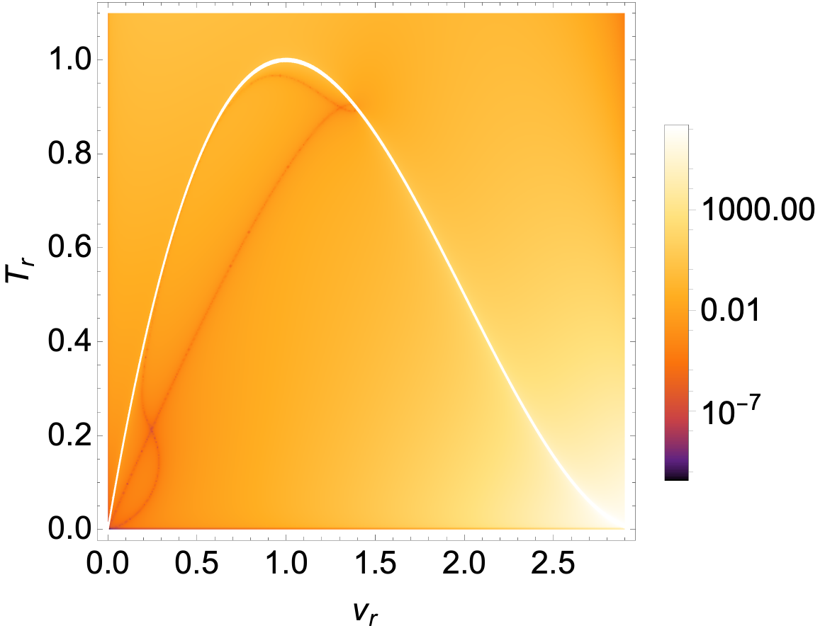
Figure 1: $\mathcal{T}$ as a function of $v_{r}$ and $T_{r}$ for the VdW model, on a logarithmic scale. The divergence of ${\mathcal{T}}$ locates the spinodal curve.

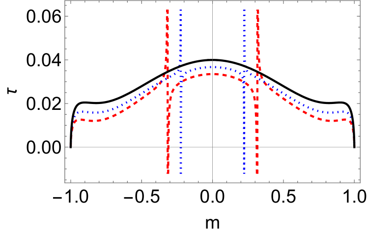
Figure 2: $\mathcal{T}$ as a function of $m$ for the Curie-Weiss model, with $T_{r}=0.9$ (dashed red), $0.95$ (dotted blue) and $0.99$ (solid black).

The behaviour of $\mathcal{T}$ is shown in Fig. 2 on a logarithmic scale, as a function of $v_{r}=1/\rho_{r}$ and $T_{r}$. The divergence of $\mathcal{T}$ along the spinodal curve can be clearly seen.

Next, we consider the Curie-Weiss (CW) ferromagnetic model, which is a symmetric cousin of the VdW model, whose information theoretic geometry was studied in JM ,tapo2 . For this model, the Helmholtz free energy per unit spin is given by

$$f_{{\rm CW}}=-k_{B}T{\rm ln}2-\frac{1}{2}k_{B}T_{c}m^{2}+\frac{k_{B}T}{2}{\rm ln}\left(1-m^{2}\right)+k_{B}Tm{\rm tanh}^{-1}m~{},$$ (28)

where, as before, $T$ is the temperature, $T_{c}$ its critical value, which we will set to unity. Also, $\left(\frac{\partial f_{{\rm CW}}}{\partial m}\right)_{T}=H$ gives the applied magnetic field, with $m$ being the magnetization per spin. It was shown in JM that the information metric is given by (setting $k_{B}=1$)

$$ds^{2}=\frac{C_{L}}{T^{2}}dT^{2}+\frac{1}{T}\frac{\left(T_{c}\left(1-m^{2}\right)-T\right)}{m^{2}-1}dm^{2}~{},$$ (29)

where $C_{L}$ is the “lattice specific heat,” an unknown function of the temperature, which arises here due to an added mechanical energy term in the CW Hamiltonian. In fact, without this somewhat ad hoc addition, information geometry becomes trivial in the CW model (see JM ). As in tapo2 , we use a convenient choice $C_{L}=1+T+T^{2}$. Our observation here is that the torsion scalar $\mathcal{T}$ is non-analytic everywhere on the spinodal curve of this model defined as $T=1-m^{2}$, but becomes regular at criticality near $m\to 0$, i.e., its scaling exponent is zero. This behaviour is straightforward to establish analytically, and is also borne out in Fig. 2 where the dashed red, dotted blue and the solid black lines correspond to $T_{r}=0.9,0.95$ and $0.99$, respectively, and the non-analyticity of the first two and the regularity of the third on the spinodal curve are apparent from this figure. Finally, we have also considered the Ising model in a transverse magnetic field tapo2 and find that the torsion scalar $\mathcal{T}$ diverges exponentially near the critical point. The computations here are similar to the other cases, and we will skip them for brevity, and will come back to this example briefly in the concluding section.

V Conclusions and discussion

The tools of information geometry have been used extensively to gain insights about coarse-grained structure of physical systems, ranging from fluids and spin chains to black holes. However, ambiguities can occur in this description due to the fact that the FIM, the primary structure used in information geometrical techniques, is a local quantity. Among different limitations, some well known ones include the emergence of the same FIM for different PDFs, as well the existence of different connections of the parameter manifold ($1$-connections, $0$-connections etc) with their corresponding Ricci scalars not always capturing the essential information about the statistical system.

As a resolution to the problem of degenerate FIM corresponding to different PDFs, in this paper we have introduced a new quantity on the parameter manifold, namely the torsion, by means of a CT of the FIM. Using the fact that the relevant scalar quantities on the parameter manifold (for example, the curvature scalar and the expansion scalar of a geodesic congruence) constructed from a metric related to the original FIM by a CT are conformally invariant due to presence of the torsion, we argue that scalar quantities constructed from the conformally related FIM carry the same physical information about the systems (via relations A to D listed in the introduction) as that of the ones constructed from the original FIM. However, due to different torsions on the parameter manifold, different PDFs can be distinguished with our construction. Furthermore, for a few statistical systems whose information geometric descriptions are well known, we have studied the nature of the torsion scalar - a new scalar quantity defined on the manifold which is independent of the FIM. While this shows a divergence all along the spinodal curve for Van der Waals fluids and has a well defined scaling relation near criticality, these features are absent for the Curie-Weiss model.

There are two caveats in our analysis which deserve further attention. First, we have taken the conformal factor to be the exponential of the thermodynamic potential, as a simple choice. Clearly, a multiplicative factor with the potential might change the results, since the potential often contains explicit logarithms. This happens, for example, in the one dimensional Ising model in a transverse field JM . It can be checked that in this case, if, for example, we take the conformal factor to be the exponential of twice the thermodynamic potential per particle, the divergence of the torsion tensor vanishes at the critical point. Such an issue is not present in the VdW and the CW models that we have studied. Secondly, as we pointed out in the introduction, in thermodynamic geometry of fluids, one demands that $R$ has the dimensions of volume. In this context, the relevance of $\mathcal{T}$ which naively has dimensions of energy per unit volume (upon suitably restoring factors of the Boltzmann constant) is less obvious and needs to be studied further.

Finally, we point out that, here we have always assumed that the metricity condition is satisfied on the parameter manifold. The extension of our method for connections with a non-metric structure as well as with torsion is left for a future work.

Appendix A Relation between FIMs for given relation between the PDFs

In this appendix we derive a relation between two FIMs corresponding to two given PDFs which are related by a function of coordinates on the parameter manifold. Let us consider two PDFs $P^{1}_{\xi}(x)$ and $P^{2}_{\xi}(x)$ which are described by same set of parameters $\xi$ and stochastic variables $x$, and assume that they are related by the following relation

$$P^{2}_{\xi}(x)=C(\xi)P^{1}_{\xi}(x)~{}.$$ (30)

Here $C(\xi)$ is solely a function of the coordinates $\xi$ of the parameter manifold. We want to find out the general relation between the FIMs constructed from them, and since the FIM carries the information contained in a given PDF it will help us to understand the nature of the PDFs as well.

The FIM corresponding to $P^{2}_{\xi}(x)$ is given by $g^{2}_{ab}=E_{\xi}[\big{(}\partial_{a}l^{2}_{\xi}\big{)}\big{(}\partial_{b}l^{2}_{\xi}\big{)}]$ and is related to the FIM corresponding to $P^{1}_{\xi}(x)$ by the relation

$$\begin{split}g^{2}_{ab}=C(\xi)~{}\int~{}dx~{}P^{1}_{\xi}(x)\Big{[}\partial_{a}\ln(C(\xi)P^{1}_{\xi}(x))\Big{]}\Big{[}\partial_{b}\ln(C(\xi)P^{1}_{\xi}(x))\Big{]}\\ =~{}~{}C\int dxP^{1}_{\xi}(x)\Big{[}\partial_{a}\ln(P^{1}_{\xi}(x))\Big{]}\Big{[}\partial_{b}\ln(P^{1}_{\xi}(x))\Big{]}+C\int dxP^{1}_{\xi}(x)\partial_{a}\ln(C)\partial_{b}\ln(C)\\ +C\int dxP^{1}_{\xi}(x)\partial_{a}\ln(C)\partial_{b}\ln(P^{1}_{\xi}(x))+C\int dxP^{1}_{\xi}(x)\partial_{a}\ln(P^{1}_{\xi}(x))\partial_{b}\ln(C)~{}.\end{split}$$ (31)

Now, using the fact that since the PDF is normalized (see Eq. (1)), its partial derivative is zero, i.e $\partial_{a}\int P^{1}_{\xi}(x)dx=0$, the last two terms of the above expression are zero, and the first two terms can be simplified to give the following simplified relation between two FIMs

$$g^{2}_{ab}(\xi)=C(\xi)~{}g^{1}_{ab}(\xi)+\frac{1}{C(\xi)}\partial_{a}C(\xi)~{}\partial_{b}C(\xi)~{}.$$ (32)

Thus if we consider two PDFs which are related to one another by a multiplicative function $C(\xi^{1},\cdots,\xi^{n})$ defined on the parameter manifold, then the two FIMs constructed from them are related by a general disformal transformation (DT). DTs are generalization of ordinary CTs and was originally considered by Bekenstein JBe . In DT two metrics are related to each other not only by a CT, but their is also an extra piece which depends on the derivative of a scalar field, which is $C(\xi)$ here. In this paper we have mainly focused on the FIMs related by a CT, however it will be interesting to consider FIMs related by a DT and see if the scalar quantities computed from them can be made disformal invariant.

References

- (1) S. I. Amari, H. Nagaoka, Methods of information geometry, O. U. P (2000).
- (2) G. Ruppeiner, A. Sahay, T. Sarkar and G. Sengupta, Phys. Rev. E 86, 052103 (2012).
- (3) A. Dey, P. Roy and T. Sarkar, Physica A 392, 6341-6352 (2013).
- (4) B. P. Dolan, Int. J. Mod. Phys. A 12, 2413 (1997).
- (5) T. Sarkar, G. Sengupta and B. Nath Tiwari, JHEP 11, 015 (2006).
- (6) T. Sarkar, G. Sengupta and B. Nath Tiwari, JHEP 10, 076 (2008).
- (7) G. Ruppeiner, A. Sahay, T. Sarkar and G. Sengupta, Phys. Rev. E 86, 052103 (2012).
- (8) G. Ruppeiner, Rev. Mod. Phys, 67, 605-59 (1995).
- (9) D. C. Brody and D. W. Hook, J. Phys. A 42, 023001 (2008).
- (10) T. Clingman, J. Murugan, J. P. Shock, arXiv:1504.03184.
- (11) J. Erdmenger, K. T. Grosvenor, and R. Jefferson, SciPost Phys. 8 (2020) no.5, 073.
- (12) J. Das Bairagya, K. Pal, K. Pal and T. Sarkar, Phys. Lett. B 805, 135416 (2020).
- (13) J. Das Bairagya, K. Pal, K. Pal and T. Sarkar, Phys. Lett. B 819, 136424 (2021).
- (14) M. Nakahara, Geometry, topology and physics, I. O. P (2003).
- (15) S. Carroll, Spacetime and Geometry - An Introduction to General Relativity, Pearson (2003).
- (16) R. M. Wald, General relativity, Chicago press (1984).
- (17) P. Kumar and T. Sarkar, Phys. Rev. E 90, no. 4, 042145 (2014).
- (18) S. Lucat, T. Prokopec, Class. Quantum Grav. 33 (2016) 245002.
- (19) T. Frankel, The Geometry of Physics : An Introduction, C. U. P (2011).
- (20) I. L. Shapiro, Phy. Rep. 357 (2002).
- (21) N. J. Poplawski, arXiv:0911.0334.
- (22) I. Quiros, Int. J. Mod. Phys. D 28(07), 1930012 (2019).
- (23) A. Golovnev, arXiv:1801.06929.
- (24) L. D. Landau, E. M. Lifshitz, “Statistical Physics Part 1, Volume 5 : Course of Theoretical Physics,” Elsevier, 2010.
- (25) H. Janyszek and R. Mrugala, Phys. Rev. A 39, 6515, (1989).
- (26) J. D. Bekenstein, Phys. Rev. D 48, 3641,(1993).