PySME

Abstract

Context. The characterization of exoplanets requires reliable determination of the fundamental parameters of their host stars. Spectral fitting plays an important role in this process. For the majority of stellar parameters, matching synthetic spectra to the observations provides a robust and unique solution for fundamental parameters, such as effective temperature, surface gravity, abundances, radial and rotational velocities and others.

Aims. Here we present a new software package for fitting high resolution stellar spectra that is easy to use, available for common platforms and free from commercial licenses. We call it PySME. It is based on the proven Spectroscopy Made Easy (later referred to as IDL SME or ”original SME”) package.

Methods. The IDL part of the original SME code has been rewritten in Python, but we kept the efficient C++ and FORTRAN code responsible for molecular-ionization equilibrium, opacities and spectral synthesis. In the process we have updated some components of the optimization procedure offering more flexibility and better analysis of the convergence. The result is a more modern package with the same functionality of the original SME.

Results. We apply PySME to a few stars of different spectral types and compared the derived fundamental parameters with the results from IDL SME and other techniques. We show that PySME works at least as well as the original SME.

1 Introduction

The determination of the fundamental stellar properties is important in many different fields of astronomy, from galactic archaeology to exoplanet studies. High resolution spectroscopy is one of the most reliable ways to determine these parameters, as it analyses the absorption features of the spectrum based on first principles. Especially with ever increasing sizes of surveys it becomes necessary to have analysis tools that can be applied to a large number of targets as well. Here we present the most recent evolution in the popular Spectroscopy Made Easy package (SME, Valenti & Piskunov 1996; Piskunov & Valenti 2017) – PySME. Previous iterations of SME were limited by the closed source IDL language in its application to large samples, this has been solved here by transitioning to Python. Additionally this allowed us to improve on some other aspects of the software as well.

PySME is one of only a few stellar spectral analysis tools available, others include Turbospectrum (Plez et al. 1993; Plez 2012b; Gerber et al. 2022), MOOG (Sneden 1973; Sneden et al. 2012), Korg (Wheeler et al. 2022), SYNSPEC (Hubeny & Lanz 2011, 2017; Hubeny et al. 2021), SYNTHE (Kurucz 1993d; Sbordone et al. 2004), and SPECTRUM (Gray & Corbally 1994).

In this paper we focus our analysis on a relatively small sample of target stars to illustrate the changes, assess the performance, and discuss some improved practical aspects of installation, use and support of this new incarnation of SME. The target stars selected here are all exoplanet host stars as those are of particular interest to exoplanet studies, but of course this new version of SME can be applied to large variety of stars, just as the existing SME.

It should be noted that exoplanet host stars have statistically higher metallicities than their non exoplanet hosting counterparts (Heiter & Luck 2003; Fischer & Valenti 2005).

The paper is divided into four parts. We start by introducing PySME, highlighting the changes and the differences from the original IDL implementation (section 2). Then we perform a comparison between the new PySME and the IDL SME implementation (section 3), to test both the accuracy of the spectral synthesis as well as the stability of the stellar parameter fitting. Afterwards we present a spectroscopic analysis carried out for a sample of planet-hosting FGK stars (section 4) and compare the results to those of other studies (section 5). Finally we analyse trends in the derived parameters and their uncertainties in relation to the stellar effective temperature (section 6), as a proxy for the stellar type.

2 PySME

SME is a spectral synthesis and fitting tool for interpretation of stellar spectra. While we focus here on exoplanet host stars exclusively, PySME is applicable to a wide variety of stars. In synthesis mode it generates a spectrum for a given set of stellar parameters ($T_{\text{eff}}$, $\log g$, abundances, macro- and micro-turbulence $v_{\text{mac}}$ and $v_{\text{mic}}$, and projected equatorial rotation velocity $v\leavevmode\nobreak\ \sin i$) for specified spectral intervals and spectral resolution (instrumental profile). In analysis mode SME finds the optimal values for selected stellar parameters that result in the best fit to the provided observations given the uncertainties of the data. The free parameters may include one or several (or even all) stellar parameters from the list above, including specific elemental abundances as well as some atomic line parameters of any transition in the line list.

The original SME package was written in IDL with the radiative transfer solver inherited from the antique FORTRAN code Synth by Piskunov (Piskunov 1992) accessed in the form of an external dynamic library. Throughout the years more and more improved and updated parts of spectral synthesis were incorporated into the library, which was later named the SME library. It currently includes the molecular-ionisation equilibrium solver EOS (Piskunov & Valenti 2017), the continuous opacity package CONTOP, the line opacity package LINOP (Barklem & Piskunov 2015), and a plane-parallel/spherical radiative transfer solver based on Bezier-spline approximation to the source functions (de la Cruz Rodríguez & Piskunov 2013).

The whole package is divided into two parts: the graphical user interface (GUI) that handles data input/output and presentation/inspection of the results, and the actual solver that either generates the synthetic spectrum or performs fitting of the observations. These two parts are communicating with each other through a data structure, known as the SME structure, which contains all the information necessary for the calculations. To initiate a process the user needs to create this structure either using the GUI or any other method. The calculation part then uses the input structure to initiate its work and upon completion packages the results into a similar output structure. The latter can explored with the GUI.

At the time of the initial development of SME, IDL was widely used in astronomy for data reduction and data analysis. Therefore only the performance-critical parts of SME were written in C and FORTRAN. However, new developments since then, such as the recent marketing policy of IDL, have motivated us to move SME to an open and free platform, such as Python. This has the benefit that PySME no longer relies on commercial software, simplifies parallelization and opens additional functionality through the use of existing Pyhthon libraries. This also simplifies the use of PySME for large surveys as was done for example for the GALAH (Buder et al. 2021) with the IDL SME. Additionally, the switch to Python offers us an opportunity to improve and modernise several of components of SME. In the following sections we will discuss in more detail specific changes that were made to PySME.

2.1 Optimization Algorithm

One of the most useful capabilities of PySME is its ability to to determine the best fit stellar parameters from comparison with an observations. In PySME this is done by solving the least squares problem:

$$\sum_{i}\text{weight}(\lambda_{i})\cdot r_{i}^{2}=\mathrm{min},$$ (1)

where the residuals $r_{i}\equiv\text{synth}(\lambda_{i},p0,p1,...)-\text{obs}(\lambda_{i})$, synth is the synthetic spectrum generated by PySME, obs is the observed spectrum, $p0,p1,...$ are the fitting parameters (e.g. effective temperature $T_{\text{eff}}$), and $\lambda_{i}$ is the wavelength of point $i$. weight is the weight of each point conventionally set to the inverse of data uncertainties $\sigma$. In IDL SME the weights where modified to include the residual intensity of observations: $\text{weight}_{i}^{2}=\text{obs}_{i}/\sigma_{i}^{2}$. In this way the optimisation algorithm is discouraged from improving the fit to the line cores at the expense of the continuum points. We find this scheme useful, in particular, when fitting a short spectral interval with comparable amount of continuum and line points and so we kept this weighing scheme in the PySME.

Instead of the Levenberg-Marquardt (LM) algorithm employed in the IDL SME, PySME uses the dogbox algorithm as described in Voglis & Lagaris (2004) and implemented in SciPy (Virtanen et al. 2020). This method is similar to the LM algorithm in that it uses both the Gauss-Newton step and the steepest decent, but it uses an explicit rectangular trust region. At each iteration it calculates the Gauss-Newton step and the steepest decent, the next step is then one of the following three options:

• If the Gauss-Newton step is within the trust region: Use the Gauss-Newton step

• If the Gauss-Newton step is outside the trust region, but the steepest decent step is inside it, use a combination of the two as shown in Figure 1.

• If both are outside the trust region: Follow the steepest decent direction to the edge of the trust region

The size of the trust region $\Delta$ is adjusted between iterations depending on the improvement of the residuals. The size of the trust region is kept constant unless the changes stop matching the linear estimate for the convergence. If the improvement is larger than expected trust region is increased. If it is marginal the trust region is decreased.

This method in our experience results in the least number of function evaluations to reach the convergence out of the methods implemented in SciPy. It also allows us to set limits on the stellar parameters without confusing the fitting process. This is occasionally required to prevent SME from extrapolating outside the grid of stellar atmospheres and keep the interpolated model physical.

Figure 1: Sketch of the dogbox algorithm in two dimensions for step $k$. The previous point is $x_{k-1}$, the next point is $x_{k}$. The rectangle represents the trust region with size $\Delta$, $\delta_{gn}$ is the Gauss-Newton step, and $t\delta_{sd}$ is the steepest decent step. Here the Gauss-Newton step falls outside the trust region, so the new step $\delta_{k}$ is a combination of both the Gauss-Newton step and the steepest decent, cut off at the boundary of the trust region.

2.2 Continuum Fitting

Correct continuum normalisation is very important for the accurate determination of stellar parameters. In PySME we achieve this by changing the continuum of the synthetic spectrum to match the observed spectrum, similar to IDL SME. Since every spectrum is different, there is no good solution that fits all situations. We therefore implement several continuum correction alternatives in PySME. A list of the methods is presented in Table 1 and a longer explanation can be found in PySME documentation. Each continuum fitting method has an associated degrees of freedom parameter, which meaning depends on the selected method. Example of some options are given in Figure 2 for an F7 dwarf HD 148816 (Houk & Swift 1999) with $T_{\text{eff}}=$5908\text{\,}$kelvin{\mathrm{K}}$$$, $\log g=$4.32\text{\,}\log\mathrm{g}$$, and $[M/H]=$-0.71\text{\,}$\mathrm{d}\mathrm{e}\mathrm{x}$$$ (Costa Silva et al. 2020).

In the mask method a user-defined mask is used to specify continuum points. Then a polynomial fit to those points is used as the continuum of the spectrum. The degree of the polynomial is a user-defined parameter. The benefit of this method is that it allows good control over the continuum placing and it works reliably if continuum points are present in selected wavelength regions. Moreover, it does not rely on the synthetic spectrum, so the continuum stays the same throughout SME iterations. The downside is the need for interactive setting of the mask and the requirement of having continuum points may be impossible to meet, e.g. for TiO molecular bands in M-dwarfs or for regions around strong lines with very broad wings.

An alternative approach is to match the relative depth of various lines to the spectral synthesis. This is implemented as match option, which uses the fact that line depth is affected non-linearly by the selected continuum level: spectral points in the center of strong lines are much less affected by a change in continuum placing than points in weak lines. Thus, the idea is to fit the continuum so that:

$$\sum_{i}\left[\text{obs}(\lambda_{i})-\text{syn}(\lambda_{i})\cdot f(\lambda_{i})\right]^{2}=\mathrm{min},$$ (2)

where $f$ is an analytical continuum function. We choose $f$ to be a polynomial and determine the coefficients using a least-squares fit. The degree of polynomial is a user-defined parameter. To match the concept of continuum PySME sets the weights for spectral points proportional to their residual intensity, so that a good continuum is found even if some lines are missing in the synthesis. This method has the advantage that it does not require the continuum points to be present in observations. On the other hand it needs the observations to represent a good range of line depths and a reasonable match to the synthetic spectrum. This frequently means fitting a relatively large spectral ranges and works best for observations with a high signal-to-noise ratio (SNR). Note, that this option requires re-evaluation of the continuum on every SME iteration. The other methods listed in Table 1 are various combinations of the mask and the match methods.

Finally, PySME can also rely on continuum normalization done before the import of observations making no continuum adjustments. Figure 2 shows some of the more successful fits to a spectral fragment for HD 148816.

Method	Description
mask	Polynomial fit to the selected points
match	Polynomial fit to match the synthetic
	and observed spectra
match+mask	Same as match, but only uses mask points
matchlines	Similar to match, but it focuses on matching the line cores instead of the continuum
matchlines+mask	Same as matchlines, but only uses mask points
spline	Similar to match, but uses a cubic spline instead of a polynomial
spline+mask	Similar to match+mask, but uses a cubic spline instead of a polynomial

Table 1: Continuum Normalization options

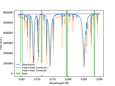
(a) mask+linear

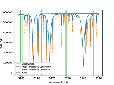
(b) mask+quadratic

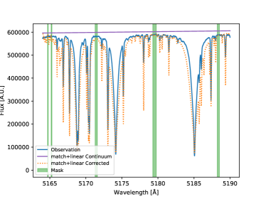
(c) match+linear

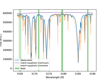
(d) match+quadratic

Figure 2: Comparison of the different continuum normalization options on a small segment of the solar spectrum. Each plot shows the original observation (blue), the corrected synthetic spectrum (dotted orange), and the continuum detected by the method (purple). The shaded regions mark the selected pixels used as the mask (green).

2.3 Radial Velocity Fitting

Just as important as the continuum is the radial velocity shift between the observed spectrum and the synthetic spectrum. The radial velocity determination can be done for each wavelength segment separately or for the entire spectrum. In PySME we determine the radial velocity in two steps. First we perform a large-range search using the cross correlation between the observed spectrum and the synthetic spectrum to get a rough estimate for the radial velocity value and avoid shallow local minima. The accuracy of this first guess is limited by the wavelength resolution of the observation as we avoid¨ interpolation and perform cross correlation data pixels. By default we limit the range of this search to $\pm 500\text{\,}\mathrm{k}\mathrm{m}\mathrm{/}\mathrm{s}$, but this value can be adjusted by the user. In a second step we refine the radial velocity value in a least squares sense, starting from the previous estimate. We shift the synthetic spectrum wavelength using the relativistic Doppler shift formula (Equation 3) in each iteration until it matches the observed spectrum.

$$\lambda^{\prime}=\lambda\sqrt{\frac{1+v/c}{1-v/c}}\ ,$$ (3)

where $\lambda^{\prime}$ is the wavelength shifted into the rest frame of the star, $\lambda$ is the wavelength in the rest frame of the observer, $v$ is the radial velocity (positive for a star moving away from the observer), and $c$ is the speed of light.

2.4 Auxiliary Data

The radiative transfer calculations at the core of SME require additional data with atomic and molecular line properties (line lists), as well as stellar model atmosphere(s). Additionally to correct for Non Local Thermal Equilibrium (NLTE) effects, PySME requires NLTE departure coefficients matching the selected atmospheric model. All of these are discussed in this section.

The line data for each transition must at least include the species name, ionisation stage, excitation energy of the lower level and the transition oscillator strength. These can be complemented by the line broadening parameters for the natural, Stark, and van der Waals broadening mechanisms. If they are not known PySME will use approximations as described in Valenti & Piskunov (1996) and Piskunov & Valenti (2017). Finally for NLTE corrections (see below), the line list should also include the term designation for the lower and upper energy levels, as well as their angular momentum quantum numbers J. Conveniently PySME supports the linelist format returned by VALD3 (Ryabchikova et al. 2015; Kupka et al. 2000, 1999; Ryabchikova et al. 1997; Piskunov et al. 1995) for the extract stellar query, which includes all required information. Both short and long formats are supported, but the long format is required for NLTE corrections.

Spectral synthesis in PySME also needs a stellar atmosphere model, which describes the temperature and pressure profiles as functions of ”depth”, where depth could be an optical depth at a standard wavelength or a column mass. When the effective temperature, surface gravity or metallicity of the synthesis does not match that of a pre-computed model, PySME interpolates in a 3-dimensional ($T_{\text{eff}}$, $\log g$, and [M/H]) grid. Grids for use with PySME are provided by several authors. These include the MARCS models (Gustafsson et al. 2008) for cool dwarf and giant stars, and ATLAS (Kurucz 2017; Heiter et al. 2002) and LL models (Shulyak et al. 2004) for hotter main sequence objects. Each model grid is packed in rather large (on the order of GB) data file and multiple grids are often available for different microturbulence parameters, alpha-element abundances etc.

To account for NLTE effects PySME uses the departure coefficient tables. Departure coefficient is the ratio between the NLTE and the LTE population of an energy level involved in radiative transition (Piskunov & Valenti 2017 describes the impact on absorption coefficient and the source function). Departure coefficient depends on the local physical conditions described by model atmosphere and the abundance of the species, responsible for absorption/emission. Thus, fitting specific abundance or/and atmospheric parameters may require interpolation. For that departure coefficients need to be computed for each layer of every atmospheric model in a grid, and for several elemental abundances around the model metallicity. The resulting data files are even larger than the model grids, and notably they can only be used with the model atmosphere grid they were calculated for.

In the original IDL SME all these files where included with the distribution package bringing its size to over 1 TB, even though most users only need a subset of this data. In PySME atmosphere model grids and departure coefficient files are instead stored on a data server until requested by the user, at which point they are automatically downloaded. This significantly reduces the installation footprint of PySME in comparison to IDL SME and, in addition this allows PySME to provide updates for these data files when available. Of course, it is still possible to add custom grids.

The new default atmosphere grid is the marcs2014 grid, which is essentially the marcs2012 grid with some holes filled and with an improved spherical models (T. Nordlander, priv. comm.). Additionally PySME also supports the latest NLTE departure coefficient grids by Amarsi et al. (2020), which have been calculated for the 2014 MARCS atmospheric grids.

2.5 Elemental Abundances

In addition to the overall metallicity, PySME also allows setting individual elemental abundances for the first $100$ elements (up to Einsteinium) manually or as a free parameter in the fitting. PySME supports abundance input following different conventions. These include the ”H=12” convention with elemental abundances set relative to Hydrogen and the ”SME” convention where abundances are set relative to the total number of atoms in a volume. Internally they are all converted to the H=12 format in the Python part of PySME, the SME library, however, uses the SME format, which was the only format used in IDL SME.

For convenience PySME supports three alternatives for ”default” solar abundances, as described in Table 2. These replace the solar abundance values of IDL SME, which was evolving with time.

Option	Source	Note
asplund2009	Asplund et al. (2009)	The default used by PySME.
grevesse2007	Grevesse et al. (2007)
lodders2003	Lodders (2003)

Table 2: Solar abundance sets included in PySME.

2.6 Convergence

We test PySME convergence to ensure the robustness of the new optimisation algorithm, i.e. we test if we get similar results for different initial sets of parameters. For this test we use a segment of the solar spectrum (4489 Å to 4603 Å) provided by the National Solar Observatory Atlas 1 (Kurucz et al. 1984), which is an optical flux spectrum for a relatively inactive Sun. We then determine the best fit $T_{\text{eff}}$, $\log g$, and [M/H], starting with different initial parameters on a 3x3x3 grid as given in Table 3. The derived parameters of these 27 runs are all within the uncertainties of the fit. In Figure 3 we show the distribution of the points in the parameter space. The standard deviation of the final values are $\sigma_{T_{\text{eff}}}=2.0$, $\sigma_{\log g}=0.005$, and $\sigma_{[M/H]}=0.001$.

Parameter	Value1	Value2	Value3
$T_{\text{eff}}$ [$\mathrm{K}$]	5000	5500	6000
$\log g$ [$\log($\mathrm{cm}\text{\,}{\mathrm{s}}^{-2}$)$]	4.0	4.4	4.8
[M/H] [$\mathrm{d}\mathrm{e}\mathrm{x}$]	-0.4	0.0	0.4

Table 3: Initial Parameters for the convergence test.

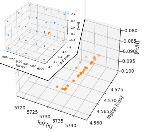
Figure 3: Distribution of the best fit stellar parameters $T_{\text{eff}}$, $\log g$, and [M/H] for different initial parameters. Initial values are shown in blue and final values in orange. The cutout in the upper left corner shows the entire parameter space spanned by the initial parameters, while the rest is zoomed in on the closely clustered final distribution.

2.7 Parameter Uncertainties

As in all parameter determinations there are two different types of uncertainties to measure. The first is the statistical uncertainty, which depends on the SNR of the observations and is easily determined from the least squares fit in PySME using the covariance matrix. We correct these uncertainties in PySME using the final $\chi^{2}$, by multiplying the covariance matrix with $\sqrt{\chi^{2}}$. This normalized the initial uncertainties on the data points to those expected for this fit.

The second uncertainty is the systematic uncertainty, which is due to inherent deficiencies of the atomic and molecular data as well as observational defects (e.g. due to incorrect parameters in the line list). These are a lot more difficult to constrain, as there is no reference for PySME to use. Instead PySME uses the uncertainty method described in Ryabchikova et al. (2016); Piskunov & Valenti (2017). This method uses the fit residuals, derivatives, and uncertainties of the observed spectrum to determine the cumulative probability distribution under the assumption that the entire residual can be explained by the variation in one parameter. Ignoring the sensitivity to other free parameters leads to an overestimation of the uncertainties. This approach works reasonable well for free parameters that explicitly affect the majority of spectral points (e.g. $T_{\text{eff}}$, [M/H]) but the estimate becomes unrealistically exaggerated for parameters affecting spectra locally ($\log g$, individual abundances). We also note here that this method is invariant to the absolute scale of the input uncertainties of the spectrum.

In 4b we show the distribution for uncertainties for $T_{\text{eff}}$ for $\epsilon$ Eri (analysis details are discussed in section 4) as cumulative probability and as probability density. Note that the central part looks reasonably close to a Gaussian distribution, which explains why we get realistic estimate for the uncertainty of $T_{\text{eff}}$. For other, more local parameters, such as individual abundances, the central part is often very asymmetric and quite different from a Gaussian.

(a) $T_{\text{eff}}$

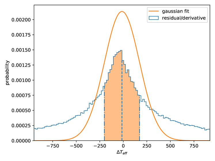
(b) $T_{\text{eff}}$

Figure 4: Cumulative probability (top) and probability density (bottom) distribution of $T_{\text{eff}}$ for a spectrum of $\epsilon$ Eri derived from the fit results (blue). For comparison we also show the distribution of a Gaussian with the same median and $\sigma$ as derived from the cumulative probability (orange). The median is marked by a dashed line (bottom), and the $1\sigma$ range is shown as dash dotted lines and a shaded region (bottom). The distributions for the other fitted stellar parameters are shown in the appendix Figure 12

.

To evaluate the accuracy of these uncertainty estimates we run a simple Monte-Carlo test. For this we create a synthetic spectrum for a single wavelength segment between $6400\text{\,}\mathrm{\text{\r{A}}}6500\text{\,}\mathrm{\text{\r{A}}}$ with stellar parameters $T_{\text{eff}}=$6000\text{\,}$kelvin{\mathrm{K}}$$$, $\log g=$4.4\text{\,}\log\mathrm{(}$\mathrm{missing}\mathrm{revert_as}\mathrm{=}{presentation}\mathrm{]}{\text{\,}\mathrm{cm}{\mathrm{s}}^{-2}}{\mathrm{cm}\text{\,}{\mathrm{s}}^{-2}}$\mathrm{)}$$, $[M/H]=$0\text{\,}$\mathrm{d}\mathrm{e}\mathrm{x}$$$. Then we apply white noise with a SNR of $100$ to this spectrum and extract the stellar parameters $T_{\text{eff}}$, $\log g$, and [M/H] using PySME with the initial parameters disturbed around the true values. Repeating this process for $1000$ we can estimate the uncertainty of the parameters from the scatter of the values. This scatter is shown in Figure 5 for $T_{\text{eff}}$, the other parameters show a similar behaviour. A comparison between the values is given in Table 4. This process does not include the systematic uncertainties of the input data as we create a synthetic spectrum to compare to, thus the uncertainties derived from the scatter match those derived by the least squares fit.

A final way to estimate the uncertainties is by comparing the results obtained here with those from previous studies (see section 6). Using the scatter of the differences we can then infer an estimate for the systematic uncertainties. The systematic uncertainties obtained this way are: $\sigma_{T_{\text{eff}}}=121$, $\sigma_{\log g}=0.16$, and $\sigma_{[M/H]}=0.07$.

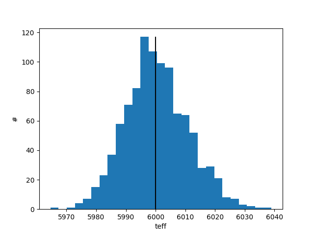
Figure 5: Scatter of the recovered $T_{\text{eff}}$ around the true value for a synthetic spectra with random noise of SNR $100$.

Parameter	$\sigma_{\text{mc}}$	$\sigma_{\text{fit}}$	$\sigma_{\text{sme}}$	$\sigma_{\text{delta}}$
$T_{\text{eff}}$ [$\mathrm{K}$]	$10.2$	$14.5$	$54$	$121$
$\log g$ [$\log($\mathrm{cm}\text{\,}{\mathrm{s}}^{-2}$)$]	$0.020$	$0.027$	$0.28$	$0.16$
[M/H] $\mathrm{d}\mathrm{e}\mathrm{x}$	$0.0065$	$0.0081$	$0.04$	$0.07$

Table 4: Comparison between the uncertainty estimates based on a synthetic spectrum. $\sigma_{\text{mc}}$ is based on the distribution of a Monte-Carlo simulation, $\sigma_{\text{fit}}$ is based on the covariance matrix of the least-squares fit, $\sigma_{\text{sme}}$ is based on the method described in subsection 2.7, and $\sigma_{\text{delta}}$ is based on the scatter of the derived values compared to the reference values from other studies in section 6.

2.8 Graphical User Interface

For PySME an entirely new graphical user interface (GUI) was developed. For improved usability it is relying on established web technologies using the Electron framework. The interface is divided into a number of sections, each managing one part of the SME structure. The spectrum section allows the user to zoom and pan on the spectra both observed and synthetic, together with the positions of the lines in the linelist. Furthermore it is possible to manually set and manipulate the bad pixel and continuum normalization mask.

The other sections can be used to change the parameters of the SME structure, including the entirety of the linelist, the elemental abundances, and the NLTE settings.

It does however not offer some of the functionality that the IDL SME GUI included. For example it is not possible to select lines directly in the spectrum, to inspect or modify their parameters. Neither is it not possible to measure the equivalent width of lines directly in the interface.

2.9 Interopability between IDL SME and PySME

PySME has been designed for an easy transition for existing IDL SME users. It is therefore capable of importing existing IDL SME input (.inp) and output (.out) structures for use with PySME or its GUI. PySME itself however uses a new file format to store those structures (.sme), which can currently not be used by IDL SME. It is possible though to create IDL readable files if an IDL installation is available on the machine using the save_as_idl function.

2.10 Parallelization

In some circumstances users may be interested in analyzing a large number of stellar spectra, e.g. in surveys. Previously this required an individual IDL license for each process that is running at the same time. This is expensive (IDL cluster license) and complicated. PySME solves both of these problems at once. Still one has to be careful, it is recommended to run each synthesis or fitting in a separate process, since the SME library should not be shared between them. Many tools exist for different systems, for example the GNU parallel tool (Tange 2011). PySME includes an easy example of such a script.

2.11 Open Source

In addition to replacing IDL with Python, which is Open Source, we also made the SME library available under the BSD 3-Clause license, which is an Open Source license. This means that you can use PySME in your projects which specify open source requirements as part of your funding, which is in line with the European Commission’s Open Science guidelines.

3 Comparison between IDL SME and PySME

With a new version of SME it is interesting to compare PySME to IDL SME, which we here split into two parts. First we assure that both versions reach the same set of free parameters (within the estimated uncertainties) given the same spectral synthesis as observations. In a second step we compare the performance, i.e. the runtime, between the two version.

3.1 Comparison of spectral synthesis

The results of the stellar synthesis are plotted in Figure 6. At first glance the two codes seem to create identical synthetic spectra, however upon closer inspection there are small numerical differences as shown in the zoom in panel for the Fe line in Figure 6. These differences are on the order of $0.01\text{\,}\%$ matching the declared precision of the radiative transfer solver included in the library. That these spectra differ by this amount is not trivial, as the Python/IDL layer of SME performs significant calculations, including the interpolation in the stellar atmosphere grid, wavelength re-sampling, disk integration with the application of macro turbulence and rotational broadening as well as the instrumental profile. We believe that the two implementations are sufficiently close as not to cause additional change that exceeds the precision of the radiative transfer solving.

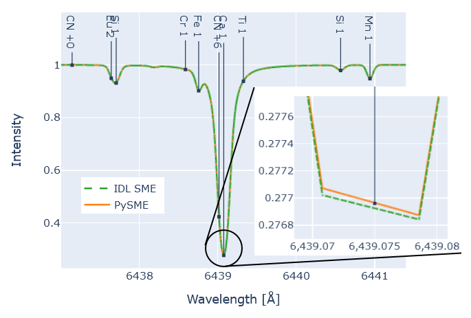
Figure 6: Comparison between the IDL SME stellar synthesis (dashed green) and the PySME stellar synthesis (orange), for a small section of the stellar spectrum. All lines in the line list are marked and labeled accordingly by vertical lines. The zoom in on the Fe line highlights the small numerical difference between the two codes.

To further convince ourselves that the new incarnation of SME performs spectral fitting at least equally well as the IDL SME we have done a blind comparison between the two. For that we used HARPS spectra of a K dwarf 55 Cnc. The IDL SME analysis was carried out by Ryabchikova (TR) while PySME fitting was done by Wehrhahn (AW). The only common parts in the two were the observations, the spectral range and the SME library. More details on the comparison and the results are presented later in subsection 4.3.

3.2 Comparison of performance

The second test concerns the speed of the calculation. For this purpose we compare the execution time for the same short spectral interval introduced in section 5 for both PySME and IDL SME. Even on the same machine the execution time varies due I/O performance and so we recorded the minimum and the average time of $1000$ runs presented in Table 5. This shows that the execution times between PySME and IDL SME are similar. Further analysis shows that the vast majority of CPU time is spent in radiative transfer calculation in the SME library, which is shared between both versions of SME.

	PySME	IDL SME
Minimum Time	$0.53\text{\,}\mathrm{s}$	$0.48\text{\,}\mathrm{s}$
Average Time	$0.75\pm 0.05\text{\,}\mathrm{s}$	$0.72\pm 0.05\text{\,}\mathrm{s}$

Table 5: Minimum and Average runtime of PySME and IDL SME on the same machine over 1000 runs. The machine runs Ubuntu and has a $3.60\text{\,}\mathrm{G}\mathrm{H}\mathrm{z}$ CPU.

4 Analysis

Finally we apply PySME to a small selection of targets. The target selection is discussed in subsection 4.1, followed by discussions on the chosen settings (subsection 4.2) and a short discussion of each target (subsection 4.3). The final parameters are given in Table 8. The results are compared to each other in section 6.

4.1 Target Selection

Determination of accurate stellar parameters for a small number of exoplanet host stars is important for interpretation of transit spectroscopy but also gives us an opportunity to assess PySME performance for a range of spectral types. Close proximity to the Sun and presence of planets makes these stars interesting and so we expected to find additional data, such as accurate parallaxes and interferometry, to help us set independent constraints on some of the stellar parameters. The selection of targets include 9 stars from the VLT CRIRES+ transit spectroscopy survey. High-quality spectra for these targets are available from ESO archive (3.6m HARPS) while interferometric radii were taken from Yee et al. (2017); von Braun et al. (2014). Table 6 summarises the data we used for the analysis.

Star	Program ID	Archive ID	S/N	Interferometry
$\epsilon$ Eri	60.A-9036(A)	ADP.2014-10-02T10:02:04.297	374	yes
HN Peg	192.C-0224(A)	ADP.2014-10-06T10:04:55.960	149	yes
HD 102195	083.C-0794(A)	ADP.2014-09-23T11:00:40.757	167	yes
HD 130322	072.C-0488(E)	ADP.2014-10-01T10:22:40.410	125	no
HD 179949	072.C-0488(E)	ADP.2014-10-02T10:00:41.887	200	no
HD 189733	072.C-0488(E)	ADP.2014-09-16T11:05:45.457	158	yes
55 Cnc	288.C-5010(A)	ADP.2014-09-26T16:51:14.897	135	yes
WASP 18	0104.C-0849(A)	ADP.2019-11-16T01:15:37.789	81	no

Table 6: List of stars analysed with PySME including the ESO program and archive IDs, average signal-to-noise ratio and the availability of reliable interferometric measurements.

4.2 Preparation of our test sample

4.2.1 Continuum

The standard HARPS pipeline does not do continuum normalisation (not required for radial velocity measurements) and thus our first task was to correct for the spectrometer blaze function and rely on PySME correction for the fine tuning as described earlier in subsection 2.2. We determine the upper envelope of the spectrum by selecting the local maxima and fitting a smooth function. The maxima are found by comparing neighbouring points, and then only keep the largest local maximum in a given interval (step size). The step size should be larger than the width of absorption features, but small enough to follow the continuum. For our data we choose the step size to be $1000$ pixels. Then we connect the selected points with straight lines and smooth the resulting curve using a Gaussian of the same width as the step size. This creates a continuous and smooth fit, that is good enough for further analysis.

The observations are then split into segments corresponding to $100\,000$ pixels each. This number is arbitrary, mostly set by easiness of inspecting the results.

When running PySME the selected linear correction of the continuum correction based on best match to the synthetic spectrum.

4.2.2 Radial Velocities

For the radial velocities we could rely on HARPS wavelength calibration and so we used a single radial velocity value for all spectral intervals.

4.2.3 Uncertainties

SME uses uncertainties of spectral points to compute the weights for the fitting procedure. The HARPS data does not contain an independent estimate of uncertainties. Only the flux value in each pixel is available. We therefore assume that the Poissonian shot noise is the only source of noise. The data has a signal-to-noise ratio on the order (or in excess) of $100$ making this a good assumption. We additionally add weight to the line centers by multiplying these uncertainties by the flux values. The final uncertainties are then:

$$\sigma=\sqrt{F_{n}}\ F_{n}\ ,$$ (4)

where $F_{n}$ is the normalized flux of the observation.

4.2.4 Tellurics

As with any ground based observation our spectra also contain telluric absorption features. We therefore provide PySME with a telluric spectrum generated with TAPAS (Bertaux et al. 2014), ignoring the Rayleigh scattering as it affects the continuum on much larger wavelength scales and will therefore be removed as part of the continuum correction. We also remove slow variations in the tellurics using the same method as for the spectrum as described in subsubsection 4.2.1. The telluric spectrum is used to mask any significant telluric lines in the observation. For this any points in the spectrum are marked as bad pixels if the tellurics are larger than $0.5$ % of the normalized spectrum.

4.2.5 Instrumental Broadening

La Silla HARPS has a slightly asymmetric instrumental profile but for our purposes deviations from a Gaussian are small and we use Gaussian broadening with a resolution of $105\,000$ to match spectral synthesis with HARPS spectra.

4.2.6 Stellar Disk Integration

Disk integration combines the rotational broadening and broadening due to radial-tangential macroturbulence. As described in section 3.3 of the original paper (Valenti & Piskunov 1996) disk integration is carried out using quadratures. For the calculations described here stellar flux spectra are computed using specific intensity at $7$ nodes (limb distances) allowing to reach the precision better than $0.1\text{\,}\%$, typically $3\cdot 10^{-4}$. Both SME implementations allow to adjust the number of nodes for better precision or faster computations while the nodes and weights are generated automatically.

4.2.7 Line list

We generate the line lists for all stars using VALD (Piskunov et al. 1995), covering the wavelength range from $3781.22\text{\,}\mathrm{\text{\r{A}}}$ to $6912.21\text{\,}\mathrm{\text{\r{A}}}$. We use the same list for all stars, which includes $52\,496$ individual lines with an expected depth of at least $1$ % at $T_{\text{eff}}$ $5770\text{\,}$kelvin{\mathrm{K}}$$, $\log g$ , [M/H] $0$, and $v_{\text{mic}}$ $1\text{\,}$\mathrm{missing}\mathrm{revert_as}\mathrm{=}{presentation}\mathrm{]}{\text{\,}\mathrm{km}{\mathrm{s}}^{-1}}{\mathrm{km}\text{\,}{\mathrm{s}}^{-1}}$$. All lines are given in the long format necessary for NLTE corrections. The line list wavelengths are in air: even though the HARPS instrument works inside a vacuum chamber, since the data reduction pipeline converts the wavelength scale of the reduced spectra to air. All references for the line parameters in each element are given in Appendix D.

4.2.8 Model Atmosphere

For the model atmosphere grid we chose the marcs2012 grid (Gustafsson et al. 2008), which is included in the PySME distribution (see subsection 2.4). We chose this grid, since it spans the parameter space of our target stars and supports the NLTE departure coefficient grids.

4.2.9 Elemental abundances

While we do fit the overall metallicity of our stars, we do not fit abundances of individual elements (even though PySME is capable of doing so). The relative abundances are instead assumed to be solar as defined by Asplund et al. (2009).

4.2.10 NLTE departure coefficients

We allow PySME to apply NLTE corrections for the $13$ elements: H, Li, C, N, O, Na, Mg, Al, Si, K, Ca, Mn, Ba using the departure coefficient grids described in Amarsi et al. (2020). In addition, Fe NLTE corrections the departure coefficients Fe described in Amarsi et al. (2016). All references for the NLTE grids are given in Appendix E.

4.2.11 Initial stellar parameters

The least squares fit requires an initial guess of the stellar parameters. The better the guess is the less iterations to determine the optimal fit parameters. The results may vary slightly depending on the of initial but, as was shown in subsection 2.6, our algorithm is quite robust and the space we explore does not contain important local minima. Thus we opted to select stellar parameters from previous studies given in the NASA Exoplanet Archive (NEXA, NASA Exoplanet Science Institute 2020) as the initial guess. The comparison of our results with NEXA parameters and alternative estimates, based on interferometric data together with the references is presented in Table 8.

4.3 Individual Targets

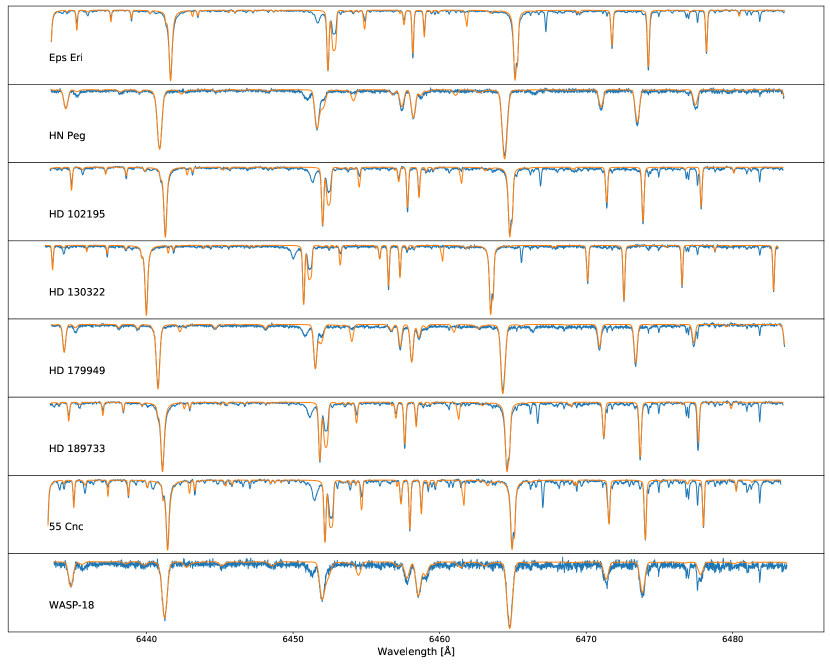
Figure 7: Observation (blue) and Synthesis (orange) flux of one wavelength section for all target stars.

We run PySME on all our targets and compare the results with IDL SME (see 55 Cnc below) and with other techniques (section 5). The free parameters were $T_{\text{eff}}$, $\log g$, [M/H], $v\leavevmode\nobreak\ \sin i$, $v_{\text{mic}}$, $v_{\text{mac}}$ and $v_{\mathrm{rv}}$. Figure 7 shows the final fit to the observations for small but representative fragment of the spectrum.

$\epsilon$ Eri is a nearby sun-like star of spectral type K2 (Keenan & McNeil 1989), with at least one planet (Mawet et al. 2019; Benedict et al. 2006; Hatzes et al. 2000) and a proposed second planet (Quillen & Thorndike 2002). $\epsilon$ Eri is one of the Gaia FGK benchmark star (Jofré et al. 2018) resulting the the following parameters: $T_{\text{eff}}$ =5076K, , $\log g$ =4.61, and [M/H] =-0.09. These are to be compared with PySME results: 4934K, 4.38, and -0.213. The HARPS data has the highest S/N in our sample so we used the example of $\epsilon$ Eri to illustrate the uncertainty estimation by PySME in subsection 2.7.

HN Peg is a star of spectral type G0 (Gray et al. 2001), with one known exoplanet (Luhman et al. 2007). Of the stars in this paper it is most similar to the Sun.

HD 102195 is a K0 star (Houk & Swift 1999), with one known exoplanet (Ge et al. 2006).

HD 130322 is another K0 star (Houk & Swift 1999), with one known exoplanet (Udry et al. 2000).

HD 179949 is an F8 star (Houk & Smith-Moore 1988), with one known exoplanet (Tinney et al. 2001).

HD 189733 is a K2 star (Gray et al. 2003) in a binary system, with one known exoplanet (Bouchy et al. 2005).

55 Cnc is a binary system with a G8-K0 dwarf (55 Cnc A, Gray et al. 2003) and an M4 dwarf (55 Cnc B, Alonso-Floriano et al. 2015). Here we investigate 55 Cnc A that is a host to a complex system of five planets (Bourrier et al. 2018). This star was independently analysed with IDL SME and so we used it the comparison between the two implementations of SME.

Observational data included several spectra of 55 Cnc obtained with the La Silla HARPS instrument on January 2012. The raw data was reduced using the standard ESO HARPS pipeline and combined to produce a single spectrum with the mean S/N of 135. We (TR) started the IDL SME analysis by manually adjusting the continuum and selecting five spectral intervals: 4900-5500 ÅÅ, 5500-5700 ÅÅ, 5700-6000 ÅÅ, 6000-6300 ÅÅ, and 6300-6700 ÅÅ. After computing a spectral synthesis based on stellar parameters taken from the literature (Udry et al. (2000)) and the VALD3 line data we have adjusted the mask of ”bad” pixels and let IDL SME do the final linear correction of the continuum level in each interval. We then solved for $T_{\text{eff}}$, $\log g$, [M/H], $v\leavevmode\nobreak\ \sin i$, and $v_{\mathrm{rv}}$. We assumed fixed $v_{\text{mic}}$ and a Gaussian instrumental profile corresponding to the resolving power of HARPS.

After this step we revisited the mask to remove poorly fitted spectral lines with obviously erroneous line data. The decision was based on comparison with the average fit quality for lines of the same species. The final step was to re-fit the parameters listed above enabling NLTE correction for Fe, Mg, Mn, Na, Si, Ba and Ca.

The PySME analysis for the comparison used the same observational data, spectral intervals, continuum normalization, mask, linelist, atmosphere grid, and NLTE departure coefficients. Thus using the same input parameters, and only comparing the results of the fitting procedure. The resulting parameters are given in Table 7 and Figure 8 shows the comparison for a fragment of spectral data included in the analysis. The difference between the best fit spectra is small and the derived parameters are compatible with each other, though not identical.

The values given in Table 8 are taken from an independent PySME analysis that follows the same steps as all other stars, i.e. has a different continuum normalization, linelist, mask, and NLTE departure coefficients than the comparison analysis.

Parameter	PySME	IDL SME
$T_{\text{eff}}$ [$\mathrm{K}$]	$5172\pm 4$	$5205\pm 30$
$\log g$ [$\log($\mathrm{cm}\text{\,}{\mathrm{s}}^{-2}$)$]	$4.17\pm 0.007$	$4.26\pm 0.09$
[M/H] $\mathrm{d}\mathrm{e}\mathrm{x}$	$0.30\pm 0.003$	$0.36\pm 0.05$
$v_{\text{mic}}$ [$\mathrm{km}\text{\,}{\mathrm{s}}^{-1}$]	$0.8$	$0.8$
$v_{\text{mac}}$ [$\mathrm{km}\text{\,}{\mathrm{s}}^{-1}$]	$3.4$	$3.4$
$v\leavevmode\nobreak\ \sin i$ [$\mathrm{km}\text{\,}{\mathrm{s}}^{-1}$]	$0.1$	$0.1$

Table 7: Stellar parameters derived from the same HARPS spectrum of 55 Cnc, in two independent analyses, one using PySME and one using IDL SME. The PySME analysis here uses different continuum normalization, linelist, mask, and NLTE departure coefficients than the analysis results shown in Table 8.

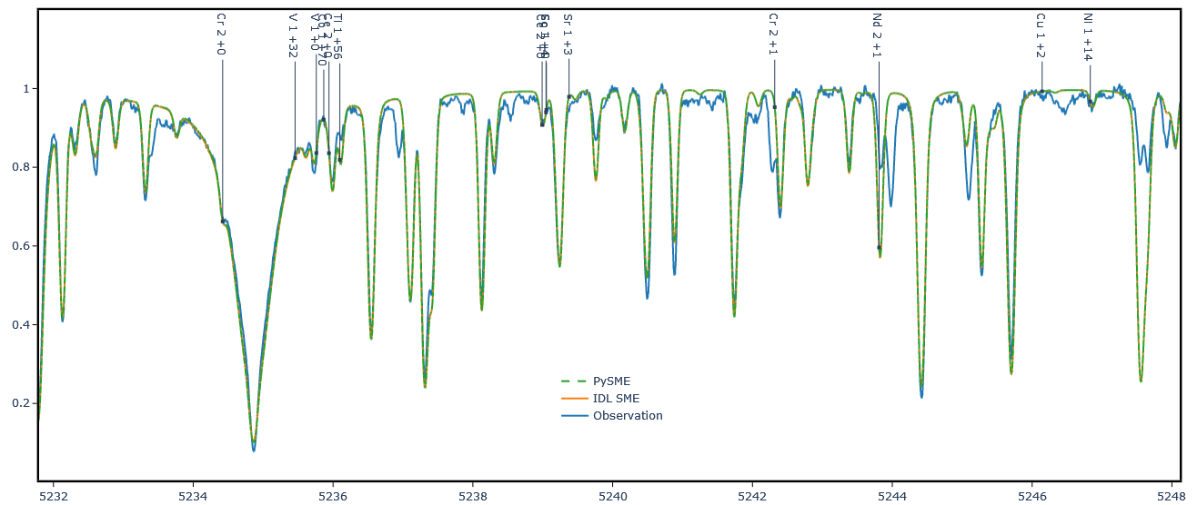
Figure 8: Comparison of the least squares fit results for 55 Cnc between the IDL SME and the PySME analysis. Both analyses used the same continuum normalization, mask, linelist, atmosphere grid, and NLTE departure coefficients. The difference between PySME and IDL SME is small, but noticeable in the derived parameters.

WASP 18 is an F6 star (Houk 1978) in a binary system, with two known exoplanets (Hellier et al. 2009; Pearson 2019). This star has the lowest SNR of the sample with a SNR of $81$.

5 Comparison with other studies

It is useful to compare the stellar parameters we derived in this study with the parameters derived in other studies. Where possible we used values derived from interferometric measurements, as those are independent from spectroscopic or photometric methods. However that is only possible for $T_{\text{eff}}$ and $\log g$, but not for metallicity. The numerical values of our results and that of other studies are given in Table 8, while we plot the differences in Figure 9. We can see that our values agree mostly with the other studies, but there appears to be some dependence on $T_{\text{eff}}$, especially for $T_{\text{eff}}$ itself. We also see a notable offset between our [M/H] and $\log g$ values and those from other studies.

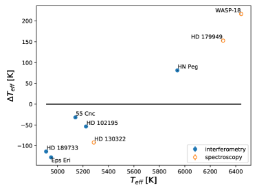
(a) $T_{\text{eff}}$

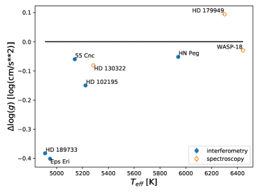
(b) $\log g$

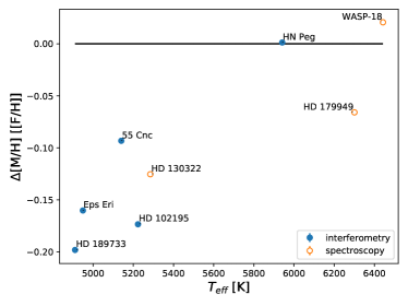
(c) [M/H]

Figure 9: Differences between the literature values and the parameter values derived in this paper. For stars represented by filled blue circles, $T_{\text{eff}}$ and $\log g$ literature values are derived from interferometry, while for stars with unfilled orange circles the literature values are derived from spectroscopy or photometry instead. Sources for all values are given in Table 8.

6 Trends

Finally it is also interesting to investigate how the uncertainties of the different parameters depend on $T_{\text{eff}}$ of the star. We therefore plot this relationship in Figure 10 for all stars. The uncertainty of the temperature depends only weakly on the temperature. Similarly the uncertainty of the surface gravity decreases slightly with temperature, while the uncertainty of the metallicity shows a stronger negative correlation. The uncertainty of the micro turbulence parameter shows no visible correlation with the temperature, while the uncertainty of the macro turbulence shows a clear upwards trend. The uncertainty of the rotation velocity decreases with increasing temperature. However there is a degeneracy with the resolution of the instrument, as below $\approx$2\text{\,}$\mathrm{missing}\mathrm{revert_as}\mathrm{=}{presentation}\mathrm{]}{\text{\,}\mathrm{km}{\mathrm{s}}^{-1}}{\mathrm{km}\text{\,}{\mathrm{s}}^{-1}}$$$ the rotational broadening is smaller than the instrumental broadening. This increases the uncertainties of $v\leavevmode\nobreak\ \sin i$ significantly for those cases.

Additionally we also compare the values of the turbulence parameters and the stellar rotation as a function of the stellar temperature in Figure 11. As expected the micro- and macroturbulence increase with the stellar temperature. The rotational velocity also increases with the stellar temperature, since rotational velocity decreases along the main sequence towards earlier spectral types (Gray 2005).

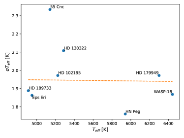
(a) $T_{\text{eff}}$

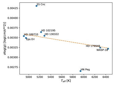
(b) $\log g$

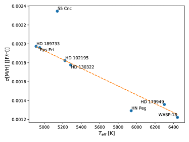
(c) [M/H]

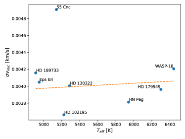
(d) $v_{\text{mic}}$

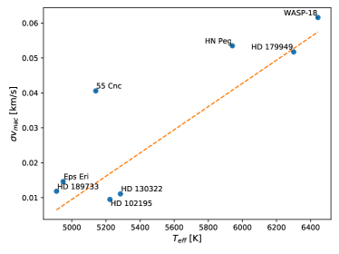
(e) $v_{\text{mac}}$

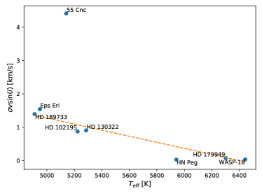
(f) $v\leavevmode\nobreak\ \sin i$

Figure 10: Uncertainty trends with the stellar temperature. Each star is marked (blue solid circle) with their names. It also shows the best fit linear relationship (orange). HN Peg and 55 Cnc are ignored in the surface gravity fit.

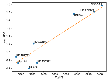
(a) $v_{\text{mic}}$

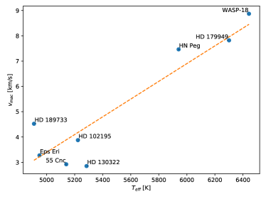
(b) $v_{\text{mac}}$

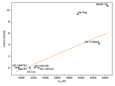
(c) $v\leavevmode\nobreak\ \sin i$

Figure 11: Micro- and macroturbulence parameters, as well as the rotational velocity, of the star, as a function of the stellar temperature. The orange dashed line shows the linear regression fit to those values.

7 Conclusion

We have shown that PySME is a suitable successor for IDL SME. We have additionally derived stellar parameters with PySME for a number of exoplanet host stars and see that their values agree both with values derived from spectroscopy, as well as independent interferometric values from other studies.

Parameter [Unit]	NEXA	Interferometry	PySME
$\epsilon$ Eri
$T_{\text{eff}}$ [$\mathrm{K}$]	5065[131][72] [1]	5077[35] [2]	$\val{4949}[2]\pm 191$
$\log g$ [$\log($\mathrm{cm}\text{\,}{\mathrm{s}}^{-2}$)$]	4.61[0.06][0.09] [1]	4.61[0.02] [2]	$\val{4.21}[0.003]\pm 0.63$
[M/H] [$\mathrm{d}\mathrm{e}\mathrm{x}$]	-0.05[0.10] [1]	-0.06[0.1] [2]	$\val{-0.22}[0.002]\pm 0.25$
$v_{\text{mic}}$ [$\mathrm{km}\text{\,}{\mathrm{s}}^{-1}$]	(1)	-	$\val{0.87}[0.004]\pm 0.7$
$v_{\text{mac}}$ [$\mathrm{km}\text{\,}{\mathrm{s}}^{-1}$]	(4)	-	$\val{3.27}[0.01]\pm 1.8$
$v\leavevmode\nobreak\ \sin i$ [$\mathrm{km}\text{\,}{\mathrm{s}}^{-1}$]	2.4[0.5] [3]	-	$\val{0.0}[4.4]\pm 189$
HN Peg
$T_{\text{eff}}$ [$\mathrm{K}$]	5927[136][155] [1]	5860[83] [2]	$\val{5941}[2]\pm 222$
$\log g$ [$\log($\mathrm{cm}\text{\,}{\mathrm{s}}^{-2}$)$]	4.46[0.08][0.09] [1]	4.43[0.05] [2]	$\val{4.37}[0.003]\pm 0.61$
[M/H] [$\mathrm{d}\mathrm{e}\mathrm{x}$]	-0.03[0.01] [1]	-0.16[0.1] [2]	$\val{-0.16}[0.001]\pm 0.18$
$v_{\text{mic}}$ [$\mathrm{km}\text{\,}{\mathrm{s}}^{-1}$]	(1)	-	$\val{1.48}[0.004]\pm 0.6$
$v_{\text{mac}}$ [$\mathrm{km}\text{\,}{\mathrm{s}}^{-1}$]	(4)	-	$\val{7.46}[0.05]\pm 5.2$
$v\leavevmode\nobreak\ \sin i$ [$\mathrm{km}\text{\,}{\mathrm{s}}^{-1}$]	8.73[0.06][0.05] [4]	-	$\val{9.29}[0.03]\pm 3.4$
HD 102195
$T_{\text{eff}}$ [$\mathrm{K}$]	5276[90][110] [1]	5277[60] [2]	$\val{5223}[2]\pm 197$
$\log g$ [$\log($\mathrm{cm}\text{\,}{\mathrm{s}}^{-2}$)$]	4.55[0.08][0.07] [1]	4.50[0.05] [2]	$\val{4.35}[0.004]\pm 0.64$
[M/H] [$\mathrm{d}\mathrm{e}\mathrm{x}$]	0.05[0.1] [1]	0.1[0.05] [2]	$\val{-0.07}[0.002]\pm 0.23$
$v_{\text{mic}}$ [$\mathrm{km}\text{\,}{\mathrm{s}}^{-1}$]	(1)	-	$\val{1.11}[0.004]\pm 0.6$
$v_{\text{mac}}$ [$\mathrm{km}\text{\,}{\mathrm{s}}^{-1}$]	(4)	-	$\val{3.87}[0.01]\pm 1.8$
$v\leavevmode\nobreak\ \sin i$ [$\mathrm{km}\text{\,}{\mathrm{s}}^{-1}$]	2.6 [5]	-	$\val{0.0}[0.9]\pm 220$
HD 130322
$T_{\text{eff}}$ [$\mathrm{K}$]	5377[132][87] [1]	-	$\val{5285}[2]\pm 212$
$\log g$ [$\log($\mathrm{cm}\text{\,}{\mathrm{s}}^{-2}$)$]	4.52[0.06][0.09] [1]	-	$\val{4.44}[0.004]\pm 0.60$
[M/H] [$\mathrm{d}\mathrm{e}\mathrm{x}$]	0.02[0.1] [1]	-	$\val{-0.11}[0.002]\pm 0.22$
$v_{\text{mic}}$ [$\mathrm{km}\text{\,}{\mathrm{s}}^{-1}$]	(1)	-	$\val{0.87}[0.004]\pm 0.6$
$v_{\text{mac}}$ [$\mathrm{km}\text{\,}{\mathrm{s}}^{-1}$]	(4)	-	$\val{2.85}[0.01]\pm 1.8$
$v\leavevmode\nobreak\ \sin i$ [$\mathrm{km}\text{\,}{\mathrm{s}}^{-1}$]	0.5[0.5] [6]	-	$\val{0.0}[0.9]\pm 167$

Parameter [Unit]	NEXA	Interferometry	PySME
HD 179949
$T_{\text{eff}}$ [$\mathrm{K}$]	6148[165][128] [1]	-	$\val{6301}[2]\pm 242$
$\log g$ [$\log($\mathrm{cm}\text{\,}{\mathrm{s}}^{-2}$)$]	4.32[0.08][0.10] [1]	-	$\val{4.41}[0.003]\pm 0.80$
[M/H] [$\mathrm{d}\mathrm{e}\mathrm{x}$]	0.2[0.1] [1]	-	$\val{0.13}[0.001]\pm 0.19$
$v_{\text{mic}}$ [$\mathrm{km}\text{\,}{\mathrm{s}}^{-1}$]	(1)	-	$\val{1.51}[0.004]\pm 0.5$
$v_{\text{mac}}$ [$\mathrm{km}\text{\,}{\mathrm{s}}^{-1}$]	(4)	-	$\val{7.82}[0.05]\pm 3.0$
$v\leavevmode\nobreak\ \sin i$ [$\mathrm{km}\text{\,}{\mathrm{s}}^{-1}$]	6.52 [7]	-	$\val{4.19}[0.07]\pm 4.7$
HD 189733
$T_{\text{eff}}$ [$\mathrm{K}$]	5023[165][119] [1]	5024[60] [2]	$\val{4910}[2]\pm 203$
$\log g$ [$\log($\mathrm{cm}\text{\,}{\mathrm{s}}^{-2}$)$]	4.58[0.08][0.12] [1]	4.51[0.05] [2]	$\val{4.12}[0.004]\pm 0.65$
[M/H] [$\mathrm{d}\mathrm{e}\mathrm{x}$]	0.20[0.10] [1]	0.07[0.05] [2]	$\val{-0.13}[0.002]\pm 0.27$
$v_{\text{mic}}$ [$\mathrm{km}\text{\,}{\mathrm{s}}^{-1}$]	(1)	-	$\val{0.94}[0.004]\pm 0.7$
$v_{\text{mac}}$ [$\mathrm{km}\text{\,}{\mathrm{s}}^{-1}$]	(4)	-	$\val{4.52}[0.01]\pm 2.1$
$v\leavevmode\nobreak\ \sin i$ [$\mathrm{km}\text{\,}{\mathrm{s}}^{-1}$]	3.5[1] [8]	-	$\val{0.0}[1.4]\pm 289$
55 Cnc
$T_{\text{eff}}$ [$\mathrm{K}$]	5250[123][172] [1]	5172[18] [2]	$\val{5140}[2]\pm 228$
$\log g$ [$\log($\mathrm{cm}\text{\,}{\mathrm{s}}^{-2}$)$]	4.42[0.05][0.14] [1]	4.43[0.02] [2]	$\val{4.37}[0.004]\pm 0.74$
[M/H] [$\mathrm{d}\mathrm{e}\mathrm{x}$]	0.35[0.10] [1]	0.35[0.10] [2]	$\val{0.26}[0.002]\pm 0.28$
$v_{\text{mic}}$ [$\mathrm{km}\text{\,}{\mathrm{s}}^{-1}$]	(1)	-	$\val{0.80}[0.005]\pm 0.7$
$v_{\text{mac}}$ [$\mathrm{km}\text{\,}{\mathrm{s}}^{-1}$]	(4)	-	$\val{2.92}[0.04]\pm 1.8$
$v\leavevmode\nobreak\ \sin i$ [$\mathrm{km}\text{\,}{\mathrm{s}}^{-1}$]	¡ 1.23[0.01] [9]	-	$\val{0.0}[4.4]\pm 189$
WASP 18
$T_{\text{eff}}$ [$\mathrm{K}$]	6226[162][117] [1]	-	$\val{6443}[2]\pm 328$
$\log g$ [$\log($\mathrm{cm}\text{\,}{\mathrm{s}}^{-2}$)$]	4.26[0.10][0.07] [1]	-	$\val{4.23}[0.003]\pm 1.01$
[M/H] [$\mathrm{d}\mathrm{e}\mathrm{x}$]	0.1[0.1] [1]	-	$\val{0.12}[0.001]\pm 0.22$
$v_{\text{mic}}$ [$\mathrm{km}\text{\,}{\mathrm{s}}^{-1}$]	(1)	-	$\val{1.58}[0.004]\pm 0.7$
$v_{\text{mac}}$ [$\mathrm{km}\text{\,}{\mathrm{s}}^{-1}$]	(4)	-	$\val{8.87}[0.06]\pm 7.3$
$v\leavevmode\nobreak\ \sin i$ [$\mathrm{km}\text{\,}{\mathrm{s}}^{-1}$]	11[1.5] [8]	-	$\val{10.7}[0.04]\pm 4.7$

Table 8: Stellar parameters of all stars investigated in this paper. For PySME both the fit uncertainty and the model uncertainty are given (see subsection 2.7). Two sets of literature values are given. The first is from the NASA Exoplanet Archive (NEXA). Those are used as initial values for the fitting procedure. The micro- and macroturbulence parameters are given in brackets () as there are no existing literature values, instead we use general estimates. In the second set of values the $T_{\text{eff}}$ and $\log g$ are derived by interferometry if that data is available, or spectroscopy otherwise. These are used in the comparison in section 6. Note that for 55 Cnc the analysis is independent of the IDL SME analysis discussed in subsection 4.3, which used a different continuum normalization, linelist, and NLTE coefficients, but instead follows the same steps as for the other targets. References: [1] Stassun et al. (2019), [2] Yee et al. (2017), [3] Valenti & Fischer (2005), [4] Swastik et al. (2021), [5] Melo et al. (2007), [6] Hinkel et al. (2015), [7] Tsantaki et al. (2014), [8] Bonomo et al. (2017), [9] Bourrier et al. (2018), [10] Gaia Collaboration et al. (2018), [11] Martioli et al. (2021), [12] Plavchan et al. (2020)

Appendix A Data Access

The input spectra are available from the ESO Archive Science Portal http://archive.eso.org/scienceportal/ with the program IDs and archive IDs given in Table 6. All generated spectra are available as SME files from Zenodo servers using DOI 10.5281/zenodo.6701350

Appendix B Installation

PySME has been developed with usability in mind. We therefore decided to make the installation process as convenient as possible. For this purpose we provide compiled versions of the SME libraries for the most common environments (windows, mac osx and linux (using the manylinux2010 specification)). Additionally we have prepared the installation via PyPi so that PySME can be installed using pip using the following command:

    pip install pysme-astro

The distribution on PyPi is automatically updated with any changes made to the open source Github repository.

In case the pre-compiled libraries are not compatible with your system it is also easy to compile the SME library from the source code.

git clone https://github.com/AWehrhahn/SMElib.git
cd SMElib
./bootstrap
./configure --prefix=$PWD
make install

This will download and compile the code on your system. Afterwards you should find the library in the lib (or bin for windows) directory. Simply copy it into your installation of PySME.

Appendix C Uncertainties

Probability distributions for the stellar parameters derived for $\epsilon$ Eri, as discussed in subsection 2.7.

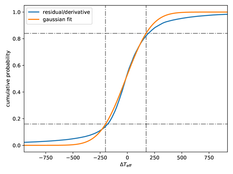
(a) $T_{\text{eff}}$

(b) $T_{\text{eff}}$

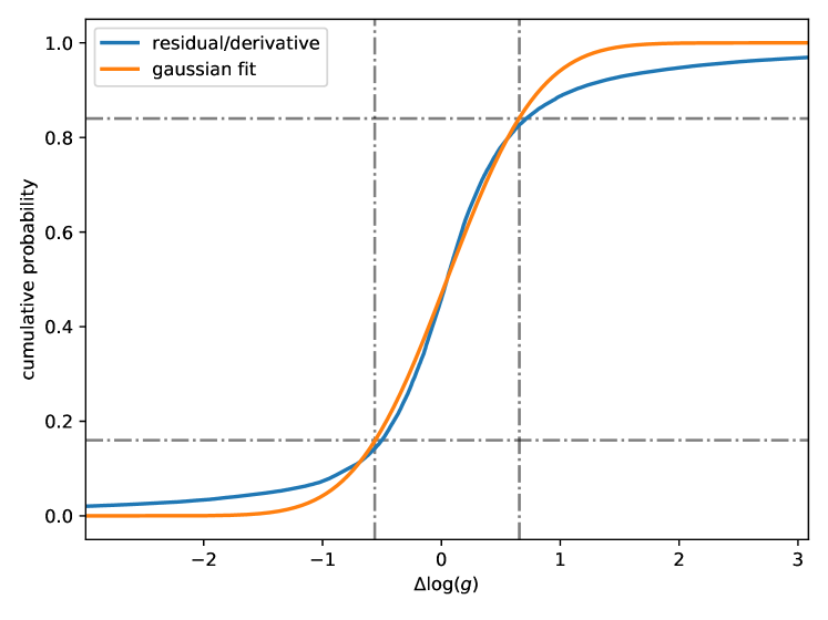
(c) $\log g$

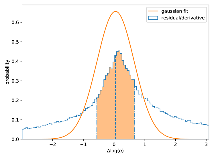
(d) $\log g$

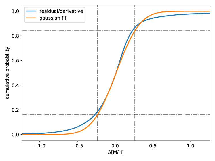
(e) [M/H]

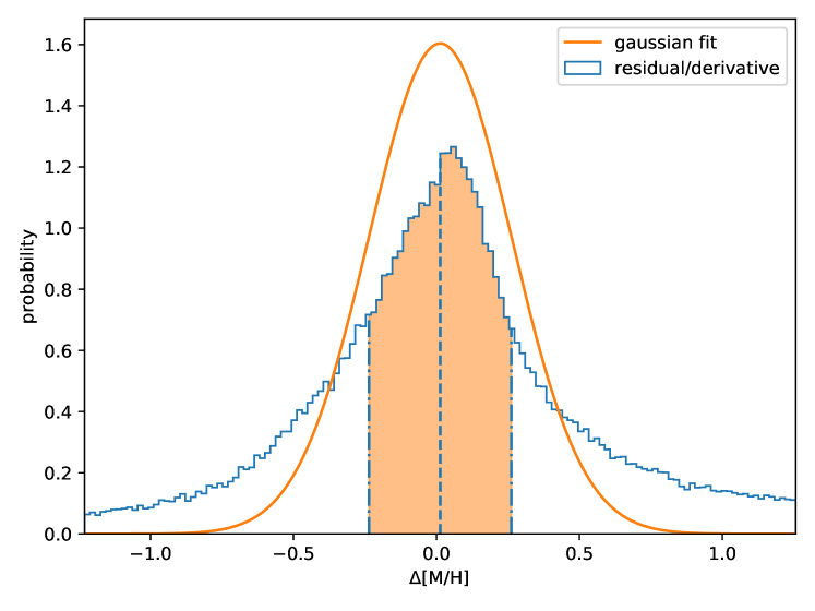
(f) [M/H]

Figure 12: Cumulative probability (left) and probability density (right) distribution of the fitting parameters for the $\epsilon$ Eri spectrum derived from the fit results (blue). For comparison we also show the distribution of a Gaussian with the same median and $\sigma$ as derived from the cumulative probability. The median is marked by a dashed line (in density plots only), and the $1\sigma$ range is shown as a shaded region and dash dotted lines.

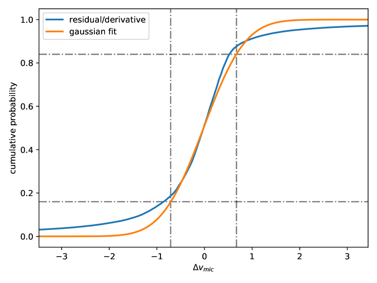
(a) $v_{\text{mic}}$

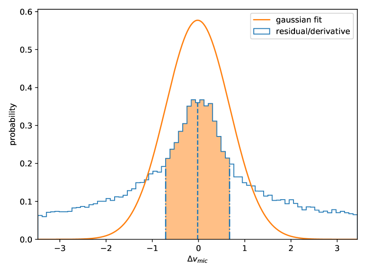
(b) $v_{\text{mic}}$

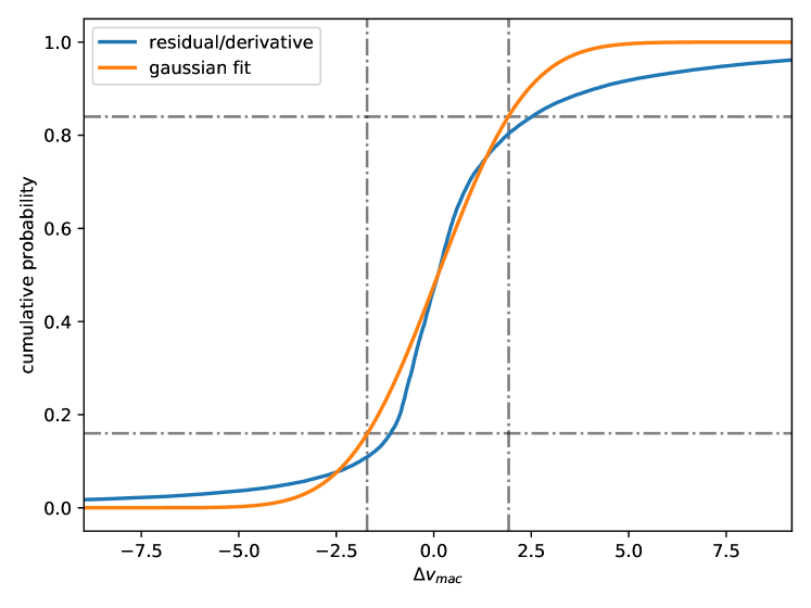
(c) $v_{\text{mac}}$

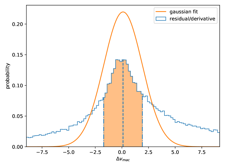
(d) $v_{\text{mac}}$

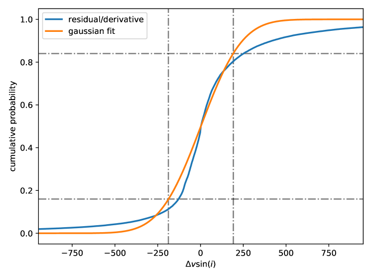
(e) $v\leavevmode\nobreak\ \sin i$

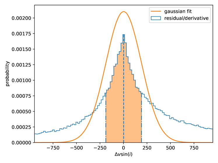
(f) $v\leavevmode\nobreak\ \sin i$

Figure 13: Continuation of Figure 12

Appendix D Line List References

Species	Reference
H 1	Kurucz 1993a
Li 1	Yan & Drake 1995
C 1	Ralchenko et al. 2010; Barklem et al. 2000
O 1	Wiese et al. 1966
Na 1	Ralchenko et al. 2010; Barklem et al. 2000; Wiese et al. 1966; Kurucz & Peytremann 1975
Mg 1	Laughlin & Victor 1974; Ralchenko et al. 2010; Anderson et al. 1967; Lincke & Ziegenbein 1971; Barklem et al. 2000; Kurucz & Peytremann 1975; Kurucz 1993b
Mg 2	Kurucz & Peytremann 1975
Al 1	Wiese et al. 1969; Kurucz 1975
Si 1	Garz 1973; Kurucz 2007
Si 2	Kurucz 2014
S 1	Kurucz 2004; Wiese et al. 1969; Biemont et al. 1993; Lambert & Warner 1968
K 1	Wiese et al. 1969
Ca 1	Smith & Raggett 1981; Kurucz 2007; Smith 1988; Barklem et al. 2000; Smith & O’Neill 1975; Drozdowski et al. 1997
Ca 2	Kurucz 2010; Seaton et al. 1994
Sc 1	Kurucz 2009; Barklem et al. 2000; Lawler & Dakin 1989; Lawler et al. 2019
Sc 2	Lawler et al. 2019; Kurucz 2009; Lawler & Dakin 1989
Ti 1	Kurucz 2016; Barklem et al. 2000; Karlsson & Litzén 2000
Ti 2	Kurucz 2016; Martin et al. 1988
V 1	Martin et al. 1988; Kurucz 2009; Barklem et al. 2000; Lawler et al. 2014
V 2	Kurucz 2010; Wood et al. 2014a; Biemont et al. 1989
Cr 1	Sobeck et al. 2007; Kurucz 2016; Barklem et al. 2000; Wallace & Hinkle 2009; Martin et al. 1988
Cr 2	Sigut & Landstreet 1990; Nilsson et al. 2006; Pinnington et al. 1993; Kurucz 2016; Gurell et al. 2010; Martin et al. 1988
Mn 1	Kurucz 2007; Den Hartog et al. 2011; Blackwell-Whitehead et al. 2005; Barklem et al. 2000; Martin et al. 1988
Mn 2	Kurucz 2009
Fe 1	O’Brian et al. 1991; Barklem et al. 2000; Kurucz 2014; Fuhr et al. 1988
Fe 2	Kurucz 2013; Fuhr et al. 1988
Co 1	Barklem et al. 2000; Lawler et al. 1990; Kurucz 2008; Fuhr et al. 1988
Co 2	Kurucz 2006
Ni 1	Wood et al. 2014b; Fuhr et al. 1988; Barklem et al. 2000; Wickliffe & Lawler 1997; Kurucz 2008
Cu 1	Kurucz 2012

Species	Reference
Zn 1	Lambert et al. 1969; Warner 1968
Ge 1	Lotrian et al. 1978
Sr 1	Corliss & Bozman 1962a; García & Campos 1988; Parkinson et al. 1976; Vaeck et al. 1988
Y 1	Kurucz 2006
Y 2	Biémont et al. 2011; Kurucz 2011
Zr 1	Corliss & Bozman 1962a; Biemont et al. 1981; Kurucz 1993c
Zr 2	Kurucz 1993c; Ljung et al. 2006; Cowley & Corliss 1983a; Biemont et al. 1981; Cowley & Corliss 1983b
Nb 1	Duquette & Lawler 1982
Mo 1	Whaling & Brault 1988
Ru 1	Wickliffe et al. 1994
Pd 1	Corliss & Bozman 1962a
Cd 1	Andersen & Soerensen 1973
In 1	Penkin & Shabanova 1963
Ba 1	Corliss & Bozman 1962a; Miles & Wiese 1969
Ba 2	Miles & Wiese 1969; Barklem et al. 2000
La 2	Lawler et al. 2001a; Corliss & Bozman 1962a; Zhiguo et al. 1999
Ce 1	Corliss & Bozman 1962a, b
Ce 2	Palmeri et al. 2000; Lawler et al. 2009
Pr 1	Meggers et al. 1975
Pr 2	Biémont et al. 2003; Ivarsson et al. 2001; Meggers et al. 1975
Nd 1	Meggers et al. 1975
Nd 2	Den Hartog et al. 2003; Xu et al. 2003; Meggers et al. 1975
Sm 1	Meggers et al. 1975
Sm 2	Meggers et al. 1975
Eu 1	Den Hartog et al. 2002
Eu 2	Lawler et al. 2001c
Gd 1	Meggers et al. 1975
Gd 2	Den Hartog et al. 2006; Meggers et al. 1975
Tb 2	Lawler et al. 2001b
Dy 1	Wickliffe et al. 2000
Dy 2	Wickliffe et al. 2000; Meggers et al. 1975
Er 1	Meggers et al. 1975
Er 2	Lawler et al. 2008; Meggers et al. 1975
Lu 1	Fedchak et al. 2000
Lu 2	Quinet et al. 1999; den Hartog et al. 1998
Hf 1	Corliss & Bozman 1962b; Duquette et al. 1982a
W 1	Obbarius & Kock 1982
Re 1	Duquette et al. 1982b
Os 1	Corliss & Bozman 1962b
Pt 1	Den Hartog et al. 2005
Tl 1	Corliss & Bozman 1962a
C2 1	Brooke et al. 2013
CH 1	Jorgensen et al. 1996
MgH 1	Kurucz 1995
TiO 1	Plez 2012a

Table 9: References for the input parameters of the line list used, sorted by element

Appendix E NLTE Grid References

Element	Reference
H	Amarsi et al. 2018b, 2020
Li	Amarsi et al. 2020; Wang et al. 2021
C	Amarsi et al. 2019, 2020
N	Lind et al. 2011; Amarsi et al. 2020
O	Amarsi et al. 2018a, 2020
Mg	Osorio et al. 2015; Amarsi et al. 2020
Al	Nordlander & Lind 2017; Amarsi et al. 2020
Si	Amarsi & Asplund 2017; Amarsi et al. 2020
K	Reggiani et al. 2019; Amarsi et al. 2020
Ca	Osorio et al. 2019; Amarsi et al. 2020
Mn	Bergemann et al. 2019; Amarsi et al. 2020
Fe	Amarsi et al. 2016
Ba	Gallagher et al. 2020; Amarsi et al. 2020

Table 10: NLTE departure coefficient grid references

References

- Alonso-Floriano et al. (2015) Alonso-Floriano, F. J., Morales, J. C., Caballero, J. A., et al. 2015, A&A, 577, A128
- Amarsi & Asplund (2017) Amarsi, A. M. & Asplund, M. 2017, MNRAS, 464, 264
- Amarsi et al. (2018a) Amarsi, A. M., Barklem, P. S., Asplund, M., Collet, R., & Zatsarinny, O. 2018a, A&A, 616, A89
- Amarsi et al. (2019) Amarsi, A. M., Barklem, P. S., Collet, R., Grevesse, N., & Asplund, M. 2019, A&A, 624, A111
- Amarsi et al. (2016) Amarsi, A. M., Lind, K., Asplund, M., Barklem, P. S., & Collet, R. 2016, MNRAS, 463, 1518
- Amarsi et al. (2020) Amarsi, A. M., Lind, K., Osorio, Y., et al. 2020, A&A, 642, A62
- Amarsi et al. (2018b) Amarsi, A. M., Nordlander, T., Barklem, P. S., et al. 2018b, A&A, 615, A139
- Andersen & Soerensen (1973) Andersen, T. & Soerensen, G. 1973, J. Quant. Spec. Radiat. Transf., 13, 369, aS
- Anderson et al. (1967) Anderson, E. M., Zilitis, V. A., & Sorokina, E. S. 1967, Optics and Spectroscopy, 23, 102, (AZS)
- Asplund et al. (2009) Asplund, M., Grevesse, N., Sauval, A. J., & Scott, P. 2009, ARA&A, 47, 481
- Astropy Collaboration et al. (2018) Astropy Collaboration, Price-Whelan, A. M., Sipőcz, B. M., et al. 2018, AJ, 156, 123
- Astropy Collaboration et al. (2013) Astropy Collaboration, Robitaille, T. P., Tollerud, E. J., et al. 2013, A&A, 558, A33
- Barklem & Piskunov (2015) Barklem, P. S. & Piskunov, N. 2015, HLINOP: Hydrogen LINe OPacity in stellar atmospheres
- Barklem et al. (2000) Barklem, P. S., Piskunov, N., & O’Mara, B. J. 2000, Astron. and Astrophys. Suppl. Ser., 142, 467, (BPM)
- Benedict et al. (2006) Benedict, G. F., McArthur, B. E., Gatewood, G., et al. 2006, AJ, 132, 2206
- Bergemann et al. (2019) Bergemann, M., Gallagher, A. J., Eitner, P., et al. 2019, A&A, 631, A80
- Bertaux et al. (2014) Bertaux, J. L., Lallement, R., Ferron, S., Boonne, C., & Bodichon, R. 2014, A&A, 564, A46
- Biémont et al. (2011) Biémont, É., Blagoev, K., Engström, L., et al. 2011, MNRAS, 414, 3350, (BBEHL)
- Biemont et al. (1989) Biemont, E., Grevesse, N., Faires, L. M., Marsden, G., & Lawler, J. E. 1989, A&A, 209, 391, (BGF)
- Biemont et al. (1981) Biemont, E., Grevesse, N., Hannaford, P., & Lowe, R. M. 1981, ApJ, 248, 867, (BGHL)
- Biémont et al. (2003) Biémont, E., Lefèbvre, P., Quinet, P., Svanberg, S., & Xu, H. L. 2003, European Physical Journal D, 27, 33, (BLQS)
- Biemont et al. (1993) Biemont, E., Quinet, P., & Zeippen, C. J. 1993, A&AS, 102, 435, (BQZ)
- Blackwell-Whitehead et al. (2005) Blackwell-Whitehead, R. J., Xu, H. L., Pickering, J. C., Nave, G., & Lundberg, H. 2005, MNRAS, 361, 1281, (BXPNL)
- Bonomo et al. (2017) Bonomo, A. S., Desidera, S., Benatti, S., et al. 2017, A&A, 602, A107
- Bouchy et al. (2005) Bouchy, F., Udry, S., Mayor, M., et al. 2005, A&A, 444, L15
- Bourrier et al. (2018) Bourrier, V., Dumusque, X., Dorn, C., et al. 2018, A&A, 619, A1
- Brooke et al. (2013) Brooke, J. S. A., Bernath, P. F., Schmidt, T. W., & Bacskay, G. B. 2013, J. Quant. Spec. Radiat. Transf., 124, 11
- Buder et al. (2021) Buder, S., Sharma, S., Kos, J., et al. 2021, MNRAS, 506, 150
- Corliss & Bozman (1962a) Corliss, C. H. & Bozman, W. R. 1962a, NBS Monograph, Vol. 53, Experimental transition probabilities for spectral lines of seventy elements; derived from the NBS Tables of spectral-line intensities (US Government Printing Office), (CB)
- Corliss & Bozman (1962b) Corliss, C. H. & Bozman, W. R. 1962b, NBS Monograph, Vol. 53, Experimental transition probabilities for spectral lines of seventy elements; derived from the NBS Tables of spectral-line intensities (Washington DC: US Government Printing Office), (CBcor)
- Costa Silva et al. (2020) Costa Silva, A. R., Delgado Mena, E., & Tsantaki, M. 2020, A&A, 634, A136
- Cowley & Corliss (1983a) Cowley, C. R. & Corliss, C. H. 1983a, MNRAS, 203, 651, (CCout)
- Cowley & Corliss (1983b) Cowley, C. R. & Corliss, C. H. 1983b, MNRAS, 203, 651, (CC)
- de la Cruz Rodríguez & Piskunov (2013) de la Cruz Rodríguez, J. & Piskunov, N. 2013, ApJ, 764, 33
- den Hartog et al. (1998) den Hartog, E. A., Curry, J. J., Wickliffe, M. E., & Lawler, J. E. 1998, Sol. Phys., 178, 239
- Den Hartog et al. (2005) Den Hartog, E. A., Herd, M. T., Lawler, J. E., et al. 2005, Astrophys. J., 619, 639, (DHL)
- Den Hartog et al. (2003) Den Hartog, E. A., Lawler, J. E., Sneden, C., & Cowan, J. J. 2003, Astrophys. J. Suppl. Ser., 148, 543, (HLSC)
- Den Hartog et al. (2006) Den Hartog, E. A., Lawler, J. E., Sneden, C., & Cowan, J. J. 2006, Astrophys. J. Suppl. Ser., 167, 292, (DLSC)
- Den Hartog et al. (2011) Den Hartog, E. A., Lawler, J. E., Sobeck, J. S., Sneden, C., & Cowan, J. J. 2011, ApJS, 194, 35, (DLSSC)
- Den Hartog et al. (2002) Den Hartog, E. A., Wickliffe, M. E., & Lawler, J. E. 2002, Astrophys. J. Suppl. Ser., 141, 255, (DHWL)
- Drozdowski et al. (1997) Drozdowski, R., Ignaciuk, M., Kwela, J., & Heldt, J. 1997, Zeitschrift fur Physik D Atoms Molecules Clusters, 41, 125, (DIKH)
- Duquette & Lawler (1982) Duquette, D. W. & Lawler, J. E. 1982, Phys. Rev. A, 26, 330, (DLa)
- Duquette et al. (1982a) Duquette, D. W., Salih, S., & Lawler, J. E. 1982a, Phys. Rev. A, 26, 2623, dSLb
- Duquette et al. (1982b) Duquette, D. W., Salih, S., & Lawler, J. E. 1982b, Journal of Physics B Atomic Molecular Physics, 15, L897, (DSLc)
- Fedchak et al. (2000) Fedchak, J. A., Den Hartog, E. A., Lawler, J. E., et al. 2000, Astrophys. J., 542, 1109, (FDLP)
- Fischer & Valenti (2005) Fischer, D. A. & Valenti, J. 2005, ApJ, 622, 1102
- Fuhr et al. (1988) Fuhr, J. R., Martin, G. A., & Wiese, W. L. 1988, Journal of Physical and Chemical Reference Data, Volume 17, Suppl.~4.~New York: American Institute of Physics (AIP) and American Chemical Society, 1988, 17, (FMW)
- Gaia Collaboration et al. (2018) Gaia Collaboration, Brown, A. G. A., Vallenari, A., et al. 2018, A&A, 616, A1
- Gallagher et al. (2020) Gallagher, A. J., Bergemann, M., Collet, R., et al. 2020, A&A, 634, A55
- García & Campos (1988) García, G. & Campos, J. 1988, J. Quant. Spec. Radiat. Transf., 39, 477, (GC)
- Garz (1973) Garz, T. 1973, A&A, 26, 471, (GARZ)
- Ge et al. (2006) Ge, J., van Eyken, J., Mahadevan, S., et al. 2006, ApJ, 648, 683
- Gerber et al. (2022) Gerber, J. M., Magg, E., Plez, B., et al. 2022, arXiv e-prints, arXiv:2206.00967
- Gray (2005) Gray, D. F. 2005, The Observation and Analysis of Stellar Photospheres (Cambridge University Press)
- Gray & Corbally (1994) Gray, R. O. & Corbally, C. J. 1994, AJ, 107, 742
- Gray et al. (2003) Gray, R. O., Corbally, C. J., Garrison, R. F., McFadden, M. T., & Robinson, P. E. 2003, AJ, 126, 2048
- Gray et al. (2001) Gray, R. O., Napier, M. G., & Winkler, L. I. 2001, AJ, 121, 2148
- Grevesse et al. (2007) Grevesse, N., Asplund, M., & Sauval, A. J. 2007, Space Sci. Rev., 130, 105
- Gurell et al. (2010) Gurell, J., Nilsson, H., Engström, L., et al. 2010, A&A, 511, A68+, (GNEL)
- Gustafsson et al. (2008) Gustafsson, B., Edvardsson, B., Eriksson, K., et al. 2008, A&A, 486, 951
- Harris et al. (2020) Harris, C. R., Millman, K. J., van der Walt, S. J., et al. 2020, Nature, 585, 357
- Hatzes et al. (2000) Hatzes, A. P., Cochran, W. D., McArthur, B., et al. 2000, ApJ, 544, L145
- Heiter et al. (2002) Heiter, U., Kupka, F., van’t Veer-Menneret, C., et al. 2002, A&A, 392, 619
- Heiter & Luck (2003) Heiter, U. & Luck, R. E. 2003, AJ, 126, 2015
- Hellier et al. (2009) Hellier, C., Anderson, D. R., Collier Cameron, A., et al. 2009, Nature, 460, 1098
- Hinkel et al. (2015) Hinkel, N. R., Kane, S. R., Henry, G. W., et al. 2015, ApJ, 803, 8
- Houk (1978) Houk, N. 1978, Michigan catalogue of two-dimensional spectral types for the HD stars
- Houk & Smith-Moore (1988) Houk, N. & Smith-Moore, M. 1988, Michigan Catalogue of Two-dimensional Spectral Types for the HD Stars. Volume 4, Declinations -26°.0 to -12°.0., Vol. 4
- Houk & Swift (1999) Houk, N. & Swift, C. 1999, Michigan Spectral Survey, 5, 0
- Hubeny et al. (2021) Hubeny, I., Allende Prieto, C., Osorio, Y., & Lanz, T. 2021, arXiv e-prints, arXiv:2104.02829
- Hubeny & Lanz (2011) Hubeny, I. & Lanz, T. 2011, Synspec: General Spectrum Synthesis Program, Astrophysics Source Code Library, record ascl:1109.022
- Hubeny & Lanz (2017) Hubeny, I. & Lanz, T. 2017, arXiv e-prints, arXiv:1706.01859
- Hunter (2007) Hunter, J. D. 2007, Computing in Science Engineering, 9, 90
- Ivarsson et al. (2001) Ivarsson, S., Litzén, U., & Wahlgren, G. M. 2001, Physica Scripta, 64, 455, (ILW)
- Jofré et al. (2018) Jofré, P., Heiter, U., Tucci Maia, M., et al. 2018, Research Notes of the American Astronomical Society, 2, 152
- Jorgensen et al. (1996) Jorgensen, U. G., Larsson, M., Iwamae, A., & Yu, B. 1996, A&A, 315, 204
- Karlsson & Litzén (2000) Karlsson, H. & Litzén, U. 2000, Journal of Physics B Atomic Molecular Physics, 33, 2929
- Keenan & McNeil (1989) Keenan, P. C. & McNeil, R. C. 1989, ApJS, 71, 245
- Kupka et al. (1999) Kupka, F., Piskunov, N., Ryabchikova, T. A., Stempels, H. C., & Weiss, W. W. 1999, A&AS, 138, 119
- Kupka et al. (2000) Kupka, F. G., Ryabchikova, T. A., Piskunov, N. E., Stempels, H. C., & Weiss, W. W. 2000, Baltic Astronomy, 9, 590
- Kurucz (1993a) Kurucz, R. 1993a, CDROM 18, SAO, Cambridge
- Kurucz (1975) Kurucz, R. L. 1975, (K75)
- Kurucz (1993b) Kurucz, R. L. 1993b, (GUES)
- Kurucz (1993c) Kurucz, R. L. 1993c, (MULT)
- Kurucz (1993d) Kurucz, R. L. 1993d, SYNTHE spectrum synthesis programs and line data
- Kurucz (1995) Kurucz, R. L. 1995, Robert L. Kurucz on-line database of molecular line lists, MgH A-X and B’-X transitions, (KMGH)
- Kurucz (2004) Kurucz, R. L. 2004, Robert L. Kurucz on-line database of observed and predicted atomic transitions
- Kurucz (2006) Kurucz, R. L. 2006, Robert L. Kurucz on-line database of observed and predicted atomic transitions
- Kurucz (2007) Kurucz, R. L. 2007, Robert L. Kurucz on-line database of observed and predicted atomic transitions
- Kurucz (2008) Kurucz, R. L. 2008, Robert L. Kurucz on-line database of observed and predicted atomic transitions
- Kurucz (2009) Kurucz, R. L. 2009, Robert L. Kurucz on-line database of observed and predicted atomic transitions
- Kurucz (2010) Kurucz, R. L. 2010, Robert L. Kurucz on-line database of observed and predicted atomic transitions
- Kurucz (2011) Kurucz, R. L. 2011, Robert L. Kurucz on-line database of observed and predicted atomic transitions
- Kurucz (2012) Kurucz, R. L. 2012, Robert L. Kurucz on-line database of observed and predicted atomic transitions
- Kurucz (2013) Kurucz, R. L. 2013, Robert L. Kurucz on-line database of observed and predicted atomic transitions
- Kurucz (2014) Kurucz, R. L. 2014, Robert L. Kurucz on-line database of observed and predicted atomic transitions
- Kurucz (2016) Kurucz, R. L. 2016, Robert L. Kurucz on-line database of observed and predicted atomic transitions
- Kurucz (2017) Kurucz, R. L. 2017, ATLAS9: Model atmosphere program with opacity distribution functions
- Kurucz et al. (1984) Kurucz, R. L., Furenlid, I., Brault, J., & Testerman, L. 1984, Solar flux atlas from 296 to 1300 nm
- Kurucz & Peytremann (1975) Kurucz, R. L. & Peytremann, E. 1975, SAO Special Report, 362, 1, (KP)
- Lambert et al. (1969) Lambert, D. L., Mallia, E. A., & Warner, B. 1969, MNRAS, 142, 71, (LMW)
- Lambert & Warner (1968) Lambert, D. L. & Warner, B. 1968, MNRAS, 138, 181, (LWa)
- Laughlin & Victor (1974) Laughlin, C. & Victor, G. A. 1974, ApJ, 192, 551, (LV)
- Lawler et al. (2001a) Lawler, J. E., Bonvallet, G., & Sneden, C. 2001a, Astrophys. J., 556, 452, (LBS)
- Lawler & Dakin (1989) Lawler, J. E. & Dakin, J. T. 1989, Journal of the Optical Society of America B Optical Physics, 6, 1457, (LD)
- Lawler et al. (2019) Lawler, J. E., Hala, Sneden, C., et al. 2019, ApJS, 241, 21
- Lawler et al. (2009) Lawler, J. E., Sneden, C., Cowan, J. J., Ivans, I. I., & Den Hartog, E. A. 2009, Astrophys. J. Suppl. Ser., 182, 51, (LSCI)
- Lawler et al. (2008) Lawler, J. E., Sneden, C., Cowan, J. J., et al. 2008, Astrophys. J. Suppl. Ser., 178, 71, (LSCW)
- Lawler et al. (1990) Lawler, J. E., Whaling, W., & Grevesse, N. 1990, Nature, 346, 635, (LWG)
- Lawler et al. (2001b) Lawler, J. E., Wickliffe, M. E., Cowley, C. R., & Sneden, C. 2001b, Astrophys. J. Suppl. Ser., 137, 341, (LWCS)
- Lawler et al. (2001c) Lawler, J. E., Wickliffe, M. E., den Hartog, E. A., & Sneden, C. 2001c, Astrophys. J., 563, 1075, (LWHS)
- Lawler et al. (2014) Lawler, J. E., Wood, M. P., Den Hartog, E. A., et al. 2014, ApJS, 215, 20
- Lincke & Ziegenbein (1971) Lincke, R. & Ziegenbein, B. 1971, Zeitschrift fur Physik, 241, 369, (LZ)
- Lind et al. (2011) Lind, K., Asplund, M., Barklem, P. S., & Belyaev, A. K. 2011, A&A, 528, A103
- Ljung et al. (2006) Ljung, G., Nilsson, H., Asplund, M., & Johansson, S. 2006, A&A, 456, 1181
- Lodders (2003) Lodders, K. 2003, ApJ, 591, 1220
- Lotrian et al. (1978) Lotrian, J., Cariou, J., Guern, Y., & Johannin-Gilles, A. 1978, Journal of Physics B Atomic Molecular Physics, 11, 2273, (LCG)
- Luhman et al. (2007) Luhman, K. L., Patten, B. M., Marengo, M., et al. 2007, ApJ, 654, 570
- Martin et al. (1988) Martin, G., Fuhr, J., & Wiese, W. 1988, J. Phys. Chem. Ref. Data Suppl., 17
- Martioli et al. (2021) Martioli, E., Hébrard, G., Correia, A. C. M., Laskar, J., & Lecavelier des Etangs, A. 2021, A&A, 649, A177
- Mawet et al. (2019) Mawet, D., Hirsch, L., Lee, E. J., et al. 2019, AJ, 157, 33
- Meggers et al. (1975) Meggers, W. F., Corliss, C. H., & Scribner, B. F. 1975, Tables of spectral-line intensities. Part I, II_- arranged by elements. (Washington DC: US Government Printing Office), (MC)
- Melo et al. (2007) Melo, C., Santos, N. C., Gieren, W., et al. 2007, A&A, 467, 721
- Miles & Wiese (1969) Miles, B. M. & Wiese, W. L. 1969, Atomic Data, 1, 1, (MW)
- NASA Exoplanet Science Institute (2020) NASA Exoplanet Science Institute. 2020, Planetary Systems Composite Table
- Nilsson et al. (2006) Nilsson, H., Ljung, G., Lundberg, H., & Nielsen, K. E. 2006, Astron. and Astrophys., 445, 1165, (NLLN)
- Nordlander & Lind (2017) Nordlander, T. & Lind, K. 2017, A&A, 607, A75
- Obbarius & Kock (1982) Obbarius, H. U. & Kock, M. 1982, Journal of Physics B Atomic Molecular Physics, 15, 527, oK
- O’Brian et al. (1991) O’Brian, T. R., Wickliffe, M. E., Lawler, J. E., Whaling, W., & Brault, J. W. 1991, Journal of the Optical Society of America B Optical Physics, 8, 1185, (BWL)
- Osorio et al. (2015) Osorio, Y., Barklem, P. S., Lind, K., et al. 2015, A&A, 579, A53
- Osorio et al. (2019) Osorio, Y., Lind, K., Barklem, P. S., Allende Prieto, C., & Zatsarinny, O. 2019, A&A, 623, A103
- Palmeri et al. (2000) Palmeri, P., Quinet, P., Wyart, J., & Biémont, E. 2000, Physica Scripta, 61, 323, (PQWB)
- Parkinson et al. (1976) Parkinson, W. H., Reeves, E. M., & Tomkins, F. S. 1976, Royal Society of London Proceedings Series A, 351, 569, (PRT)
- Pearson (2019) Pearson, K. A. 2019, AJ, 158, 243
- Penkin & Shabanova (1963) Penkin, N. P. & Shabanova, L. N. 1963, Optics and Spectroscopy, 14, 5, (PSa)
- Pinnington et al. (1993) Pinnington, E. H., Ji, Q., Guo, B., et al. 1993, Canadian Journal of Physics, 71, 470, (PGBH)
- Piskunov & Valenti (2017) Piskunov, N. & Valenti, J. A. 2017, A&A, 597, A16
- Piskunov (1992) Piskunov, N. E. 1992, in Physics and Evolution of Stars: Stellar Magnetism, 92
- Piskunov et al. (1995) Piskunov, N. E., Kupka, F., Ryabchikova, T. A., Weiss, W. W., & Jeffery, C. S. 1995, A&AS, 112, 525
- Plavchan et al. (2020) Plavchan, P., Barclay, T., Gagné, J., et al. 2020, Nature, 582, 497
- Plez (2012a) Plez, B. 2012a, (PPN2012)
- Plez (2012b) Plez, B. 2012b, Turbospectrum: Code for spectral synthesis, Astrophysics Source Code Library, record ascl:1205.004
- Plez et al. (1993) Plez, B., Smith, V. V., & Lambert, D. L. 1993, ApJ, 418, 812
- Quillen & Thorndike (2002) Quillen, A. C. & Thorndike, S. 2002, ApJ, 578, L149
- Quinet et al. (1999) Quinet, P., Palmeri, P., Biémont, E., et al. 1999, Monthly Notices Roy. Astron. Soc., 307, 934, (QPBM)
- Ralchenko et al. (2010) Ralchenko, Y., Kramida, A., Reader, J., & NIST ASD Team. 2010, NIST Atomic Spectra Database (ver. 4.0.0), [Online].
- Reggiani et al. (2019) Reggiani, H., Amarsi, A. M., Lind, K., et al. 2019, A&A, 627, A177
- Ryabchikova et al. (2015) Ryabchikova, T., Piskunov, N., Kurucz, R. L., et al. 2015, Physica Scripta, 90, 054005
- Ryabchikova et al. (2016) Ryabchikova, T., Piskunov, N., Pakhomov, Y., et al. 2016, MNRAS, 456, 1221
- Ryabchikova et al. (1997) Ryabchikova, T. A., Piskunov, N. E., Kupka, F., & Weiss, W. W. 1997, Baltic Astronomy, 6, 244
- Sbordone et al. (2004) Sbordone, L., Bonifacio, P., Castelli, F., & Kurucz, R. L. 2004, Memorie della Societa Astronomica Italiana Supplementi, 5, 93
- Seaton et al. (1994) Seaton, M. J., Yan, Y., Mihalas, D., & Pradhan, A. K. 1994, Monthly Notices Roy. Astron. Soc., 266, 805, (TB)
- Shulyak et al. (2004) Shulyak, D., Tsymbal, V., Ryabchikova, T., Stütz, C., & Weiss, W. W. 2004, A&A, 428, 993
- Sigut & Landstreet (1990) Sigut, T. A. A. & Landstreet, J. D. 1990, MNRAS, 247, 611, (SLd)
- Smith (1988) Smith, G. 1988, Journal of Physics B Atomic Molecular Physics, 21, 2827, (S)
- Smith & O’Neill (1975) Smith, G. & O’Neill, J. A. 1975, Astron. and Astrophys., 38, 1, (SN)
- Smith & Raggett (1981) Smith, G. & Raggett, D. S. J. 1981, Journal of Physics B Atomic Molecular Physics, 14, 4015, (SR)
- Sneden (1973) Sneden, C. 1973, ApJ, 184, 839
- Sneden et al. (2012) Sneden, C., Bean, J., Ivans, I., Lucatello, S., & Sobeck, J. 2012, MOOG: LTE line analysis and spectrum synthesis, Astrophysics Source Code Library, record ascl:1202.009
- Sobeck et al. (2007) Sobeck, J. S., Lawler, J. E., & Sneden, C. 2007, Astrophys. J., 667, 1267, (SLS)
- Stassun et al. (2019) Stassun, K. G., Oelkers, R. J., Paegert, M., et al. 2019, AJ, 158, 138
- Swastik et al. (2021) Swastik, C., Banyal, R. K., Narang, M., et al. 2021, AJ, 161, 114
- Tange (2011) Tange, . 2011, login: The USENIX Magazine, 42
- Tinney et al. (2001) Tinney, C. G., Butler, R. P., Marcy, G. W., et al. 2001, ApJ, 551, 507
- Tsantaki et al. (2014) Tsantaki, M., Sousa, S. G., Santos, N. C., et al. 2014, A&A, 570, A80
- Udry et al. (2000) Udry, S., Mayor, M., Naef, D., et al. 2000, A&A, 356, 590
- Vaeck et al. (1988) Vaeck, N., Godefroid, M., & Hansen, J. E. 1988, Phys. Rev. A, 38, 2830, (VGH)
- Valenti & Fischer (2005) Valenti, J. A. & Fischer, D. A. 2005, ApJS, 159, 141
- Valenti & Piskunov (1996) Valenti, J. A. & Piskunov, N. 1996, A&AS, 118, 595
- Virtanen et al. (2020) Virtanen, P., Gommers, R., Oliphant, T. E., et al. 2020, Nature Methods, 17, 261
- Voglis & Lagaris (2004) Voglis, C. & Lagaris, I. E. 2004, in WSEAS International Conference on APPLIED MATHEMATICS
- von Braun et al. (2014) von Braun, K., Boyajian, T. S., van Belle, G. T., et al. 2014, MNRAS, 438, 2413
- Wallace & Hinkle (2009) Wallace, L. & Hinkle, K. 2009, ApJ, 700, 720
- Wang et al. (2021) Wang, E. X., Nordlander, T., Asplund, M., et al. 2021, MNRAS, 500, 2159
- Warner (1968) Warner, B. 1968, MNRAS, 140, 53, wa
- Wes McKinney (2010) Wes McKinney. 2010, in Proceedings of the 9th Python in Science Conference, ed. Stéfan van der Walt & Jarrod Millman, 56 – 61
- Whaling & Brault (1988) Whaling, W. & Brault, J. W. 1988, Phys. Scr, 38, 707, (WBb)
- Wheeler et al. (2022) Wheeler, A. J., Abruzzo, M. W., Casey, A. R., & Ness, M. K. 2022, arXiv e-prints, arXiv:2211.00029
- Wickliffe & Lawler (1997) Wickliffe, M. E. & Lawler, J. E. 1997, ApJS, 110, 163, (WLa)
- Wickliffe et al. (2000) Wickliffe, M. E., Lawler, J. E., & Nave, G. 2000, J. Quant. Spectrosc. Radiat. Transfer, 66, 363, (WLN)
- Wickliffe et al. (1994) Wickliffe, M. E., Salih, S., & Lawler, J. E. 1994, J. Quant. Spec. Radiat. Transf., 51, 545, (WSL)
- Wiese et al. (1966) Wiese, W. L., Smith, M. W., & Glennon, B. M. 1966, Atomic transition probabilities. Vol.: Hydrogen through Neon. A critical data compilation (US Government Printing Office), (WSG)
- Wiese et al. (1969) Wiese, W. L., Smith, M. W., & Miles, B. M. 1969, Atomic transition probabilities. Vol. 2: Sodium through Calcium. A critical data compilation (US Government Printing Office), (WSM)
- Wood et al. (2014a) Wood, M. P., Lawler, J. E., Den Hartog, E. A., Sneden, C., & Cowan, J. J. 2014a, ApJS, 214, 18
- Wood et al. (2014b) Wood, M. P., Lawler, J. E., Sneden, C., & Cowan, J. J. 2014b, ApJS, 211, 20
- Xu et al. (2003) Xu, H. L., Svanberg, S., Cowan, R. D., et al. 2003, Monthly Notices Roy. Astron. Soc., 346, 433, (XSCL)
- Yan & Drake (1995) Yan, Z.-C. & Drake, G. W. F. 1995, Phys. Rev. A, 52, 4316, (YD)
- Yee et al. (2017) Yee, S. W., Petigura, E. A., & von Braun, K. 2017, ApJ, 836, 77
- Zhiguo et al. (1999) Zhiguo, Z., Zhongshan, L., & Zhankui, J. 1999, European Physical Journal D, 7, 499, (ZZZ)