Multi-mode fiber reservoir computing overcomes shallow neural networks classifiers

Abstract

In the field of disordered photonics, a common objective is to characterize optically opaque materials for controlling light delivery or performing imaging. Among various complex devices, multi-mode optical fibers stand out as cost-effective and easy-to-handle tools, making them attractive for several tasks. In this context, we leverage the reservoir computing paradigm to recast these fibers into random hardware projectors, transforming an input dataset into a higher dimensional speckled image set. The goal of our study is to demonstrate that using such randomized data for classification by training a single logistic regression layer improves accuracy compared to training on direct raw images. Interestingly, we found that the classification accuracy achieved using the reservoir is also higher than that obtained with the standard transmission matrix model, a widely accepted tool for describing light transmission through disordered devices. We find that the reason for such improved performance could be due to the fact that the hardware classifier operates in a flatter region of the loss landscape when trained on fiber data, which aligns with the current theory of deep neural networks. These findings strongly suggest that multi-mode fibers possess robust generalization properties, positioning them as promising tools for optically-assisted neural networks. With this study, in fact, we want to contribute to advancing the knowledge and practical utilization of these versatile instruments, which may play a significant role in shaping the future of machine learning.

Keywords

Multi-mode fibers, reservoir computing, disordered photonics,

neural networks, classification, MNIST.

I Introduction

A sound understanding of the huge success of Neural Networks (NNs) in learning processes and inference tasks is still lacking. A fundamental point is to understand why such architectures, that can have even billions of parameters, do not severely overfit data, as predicted by statistical learning theory and the so-called bias-variance tradeoff (see for example Hastie et al. (2003) or MacKay (2003)). The abundance of learnable parameters, in fact, is arguably the most universal feature in the zoo of NN architectures. Interestingly, it is known that, once the NN architecture is set, most of the model parameters adapts little-to-nothing during the learning procedure Chizat et al. (2019); Geiger et al. (2020), suggesting that random projections may play an equally important role in NNs. Recent works, in fact, have shown that it is possible to train a simple two-layer model by learning only the upper layer, interpreting the first one as a random projection Gerace et al. (2020); Goldt et al. (2022). These results were further strengthened by Baldassi et al. Baldassi et al. (2022), who proved that increasing the dimension of the random projection leads to the production of special states in the loss landscape (the function that is minimized during the training of the model), which are related to the good generalization properties in neural networks. Finally, recent evidence is provided Perugini and et al. that the way the random projection is chosen is fundamental to determine the generalization properties of the upper layer of these simple models. This suggests that different classes of random (possibly non-linear) projections impact differently on the performance of the models.

In this context, we are interested in the study of hardware random projectors such are those employed in the field of photonic neuromorphic computing Wetzstein et al. (2020); De Marinis et al. (2019). The advantages of using optical neural networks (ONN) is that neurons can be made interact by exploiting light scattering Lin et al. (2018); Zhou et al. (2021); Li et al. (2021) and photon interference Abu-Mostafa and Psaltis (1987); Shen et al. (2017) at the speed of light. Tools for shaping and controlling the light-field Dong et al. (2019) are becoming so versatile that the field is under constant development, aiming at high-speed, high-throughput optical-based computing architectures. All-optical neural networks Lin et al. (2018); Luo et al. (2019), in particular, have the potential to be great tools for fast computation, but they require an accurate modeling of the optical system to perform consistent back-propagation update Spall et al. (2022). However, the fine-tuning of the optical parameters is challenging due to discrepancies between the response of the real system and the physical model employed to describe the architecture. This reality gap often reduces the expected performance of the network Zuo et al. (2019); Wright et al. (2022), requiring additional corrections at software-level Zhou et al. (2021), training enforcement via hybrid strategies Spall et al. (2022), or employing NNs to more accurately model the optical response of the system Wright et al. (2022). Instead of modeling the physical systems, the reservoir computing (RC) Tanaka et al. (2019) approach directly make use of the non-linear outputs determined by the physics of the hardware itself. In simple words, RC relies on the fact that the hardware is able to do some unknown -but pre-determined and stable- computation, yielding a highly non-linear response. Due to this, RCs are employed typically to perform a given task (i.e., classification Saade et al. (2016); Ballarini et al. (2020)) by training a single layer that uses the output response of the reservoir as its input dataset. Some relevant applications make use of highly non-linear physical systems (such as polaritons Ballarini et al. (2020), disordered dopant-atom network Chen et al. (2020), dynamic memristors Du et al. (2017)) but require low temperature, sensitive alignment, and expensive hardware.

In this rapidly evolving scenario, the class of random projections realized by multi-mode fibers (MMF) are promising candidates for realizing reservoir-based ONNs. The optical modes entering the MMF are, in fact, mixed together in a way that is conceptually similar to what a fully connected layer with random weights does. These devices scramble the photons due to scattering events occurring during the light-field propagation, yielding to the formation of speckle patterns that are, in fact, random projections. Although the light transmission can be regarded as a linear process Popoff et al. (2010a), interference takes place when dealing with the measurement of the light-field intensity. Since the detection is nonlinear, MMFs can be used in reservoir mode to classify time-domain waveforms (using saturation effects as further nonlinearity) Paudel et al. (2020), in pattern classification of 2-bits sequences Porte et al. (2021), or for binary (human, not human) facial recognition Takagi et al. (2017). Furthermore, when dealing with more complex classification tasks, high-power laser pulses were employed to trigger the nonlinear response of the fiber itself Teğin et al. (2021). Due to the increasing interest in the employment of MMFs as reservoir, we decided to study their behavior in carrying out classification tasks in a linear, low-power continuum regime, expanding the prior work that employed a generic random medium Saade et al. (2016).

We do this by comparing the performance of the physical ONN to that obtained with random Gaussian linear projections and to that of a transmission matrix approach, the model commonly used to describe light propagation in disordered structures Popoff et al. (2010a); Ancora and Leuzzi (2022). We perform our study statistically, shuffling the training set to assess the average behavior of the RC under different training and initialization conditions. Remarkably, a single MMF provides simultaneously two independent (though deterministically linked) projections at both edges of the fiber, which we study separately using different saturation regimes. Here, we show that the MMF leads to accuracy higher than its corresponding transmission matrix model that fit for its characterization, highlighting the reality gap between model theory and experimental results. To assess the reason of this performance gap, we study the characteristic of complex-valued random projections in terms of flatness of the local energy landscape, proving that the MMF projection is more robust than those provided by alternative datasets. Additionally, we characterize the behavior of a hardware-based neural network using optical fibers in terms of the numbers of the modes employed in the reservoir. We have set up our study not for achieving the best performance in classification tasks, but rather to deepen the understanding of physical neural networks against their physical model, giving insights on the usage of MMF fibers for optical computation.

II Materials and Methods

In a low-power regime, a generic multi-mode fiber transports the electromagnetic field via a linear process Popoff et al. (2010a) so that the light propagation can be described using a simple multiplication of the input signal by a matrix that encodes the transmission rule:

$$\textbf{y}=\mathbb{T}\textbf{x}.$$ (1)

In this descriptive model, x is the controlled input, $\mathbb{T}$ is the (complex-valued and typically unknown) transmission matrix of the medium, and y is the output field. Despite its propagation, the way we measure the MMF output is not linear for two reasons. First, photons carry complex signals, i.e., the electromagnetic field associated to each propagation mode is characterized by amplitude and phase. Current electronic devices cannot follow the rapid oscillation of the field, which makes impossible the measure of the phase information. Assuming also the possibility that the readout also is perturbed by an additive noise $\varepsilon$, the camera only sees the intensity distribution:

$$\left|\textbf{y}\right|^{2}=\left|\mathbb{T}\textbf{x}\right|^{2}+\varepsilon.$$ (2)

Second, the camera has a well defined sensitivity range that depends on each pixels capability to store intensity change. If the signal reaching a given pixel exceeds the sensitivity, the measure gets clipped at the peak (overexposure) or at the bottom (underexposure). In analogy to machine learning terminology, the measuring process can be described by a non-linear activation function $\sigma(\cdot)$ that acts on the result of a complex-valued linear transmission, $\mathbb{T}\textbf{x}$. For instance, the camera recording process can be represented using the saturating linear transfer function (SatLin):

$$\sigma\left(\mathbb{T}\textbf{x}\right)=\min\left(\max\left(d,\left|\mathbb{T}\textbf{x}\right|^{2}+\varepsilon\right),2^{b}-1\right),$$ (3)

where the quantity $d$ is the intensity threshold under which the measure is not recorded, and $b$ is the bit depth of the camera.

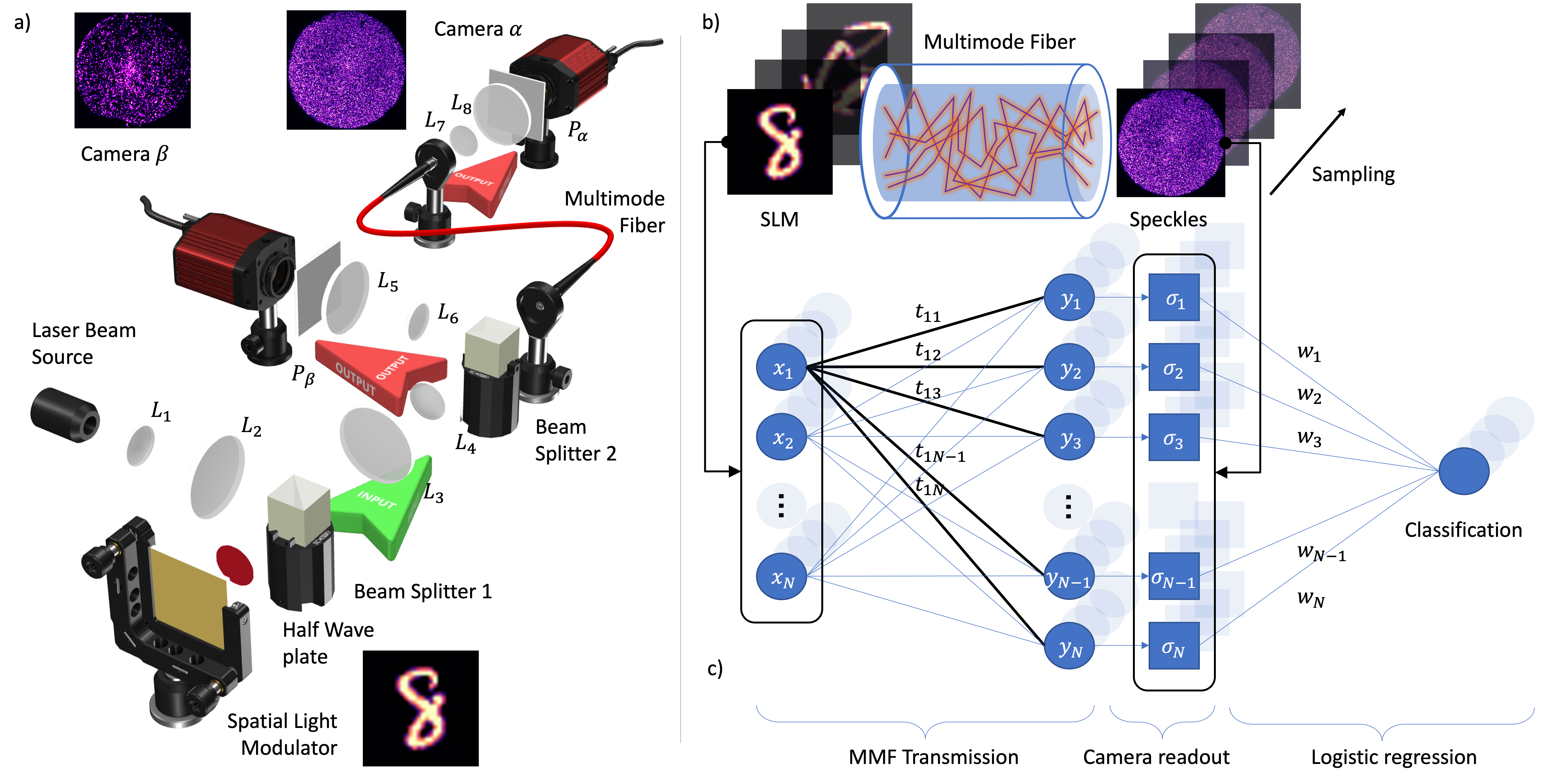
Figure 1: Schematics of the shallow optical neural network with the MMF. Panel a), simplified scheme of light transport through multi-mode fibers. The MNIST data set, modulated by a spatial light modulator, enters the MMF on the input facet. During propagation, the light gets scrambled with a random but deterministic process, giving rise to the speckle pattern measured in the camera. Panel b), corresponding neural network interpretation of the light propagation scheme. The MNIST set constitutes the input vector of a linear complex layer with static weights. The non-linear operation is determined by the camera that reads the intensity of a complex field. Successively, a linear classification layer is trained using the output of the fiber. Panel c), scheme of the imaging setup.

These considerations make the readout of a coherent field non-linear, as well as its inverse transmission recovery problem van Putten and Mosk (2010); Popoff et al. (2010a, b); Aulbach et al. (2011); Popoff et al. (2014); Rotter and Gigan (2017); Ancora and Leuzzi (2022). Such matrix can be estimated by using the four-phases method Popoff et al. (2010a), Bayesian optimization Drémeau et al. (2015), or iterative Gerchberg-Saxton schemes Huang et al. (2021); Ancora et al. (2022). However, the characterization of the device in terms of its transmission rule is not the scope of this paper, nor to circumvent the limitations of the measuring process. Instead, we want to study the multi-modal random-projection nature of the fiber to perform reservoir computing. In reservoir mode, the fiber can be seen as an optical analogous of a pre-trained fully-connected network composed by a single “hidden layer”. In this shallow architecture, the MMF layer already contains a particular realization of static weights (the reservoir, i.e., the transmission $\mathbb{T}$), which depends upon the physical status of the optical fiber. This property allows to perform random -but deterministic- projections at the speed of light using a fixed transmission rule, which can be read out by the camera. Given these considerations, the MMF is a good candidate to perform non-linear optical computation using continuous laser source even using inexpensive and large (thus easier to handle in a setup) optical multi-mode fibers. In particular, if we let just a few modes propagate into the input facet of an MMF that supports many more, all the output modes will be activated, implying a mapping of the kind few-to-many. In this latter case, the optical hidden layer (i.e., MMF and camera) can perform fully-connected random projections on a higher dimensional space.

III Results and Discussions

The goal of this study is to carry out image classification by concatenating a software-trained linear layer to the measured output of a MMF, produced by inserting a given image from the dataset into the input edge of the fiber. We choose to approach the MNIST classification problem in order to carry out a widely studied non-linear task. The only parameters that we train are those of a simple logistic regression layer, which is known to achieve poor performances on the standard MNIST set, reaching a maximum classification accuracy of 92.7% Ballarini et al. (2020). Exploiting random projection provided by the MMF, an optical device that is known to be linear, we compare with the performances obtained using reference datasets. In this study, we train the parameters of the logistic classifier using six different input datasets:

1. Original MNIST. The standard MNIST dataset, constituted by images of $l\times l$ pixels. The accuracy performance of this set is the baseline of our study.

2. Randomized MNIST. The MNIST set is linearly multiplied with a Gaussian random matrix with positive entries. This maps the dataset into a higher-dimension space, producing images with a side $L\gg l$ pixels.

3. Upscaled MNIST. Each image at the original resolution is expanded by a factor $L/l$ using a linear spline interpolation to reach the target size of $L\times L$.

4. MMF $\alpha$-cam. The speckled output of the MMF is recorded with a resolution of $L\times L$ pixels. Each speckle pattern is the result of sending a MNIST image (of size $l\times l$) on the input edge of the fiber, recording the output after disordered propagation.

5. MMF $\beta$-cam. Same as the previous one, with the speckles being recorded on the same input facet as that of the light injection. A relatively small portion of the light propagating forward is internally reflected and comes back towards the input edge. This determines a different speckle realization that we acquire as an independent measurement.

6. Simulated MMF. The transmission is characterized retrieving its corresponding matrix $\mathbb{T}$ using the SmoothGS protocol Ancora et al. (2022). The inferred transmission is used to simulate the propagation of the MNIST set using Eq. (1), recording the simulated speckle pattern by storing only the squared modulus.

All the datasets were used for a supervised training, in which the image of the MNIST set is associated to the number that represents, and the speckle image is associated to the classified number corresponding to the MNIST image impinged onto the fiber. Further details of the training procedure can be found in the Appendix section .1. To isolate a possible dependence on the problem size, we choose to set the size of the randomized and up-scaled MNIST sets to have the same dimension as the recorded fiber output. This implies that the same number of parameters are trained while solving the classification problem for every dataset, the only exception being the original set. In the following, we report the average results obtained by running independent logistic regressions on each dataset, comparing the classification accuracy on a test-set composed by $1000$ numbers isolated from the original one.

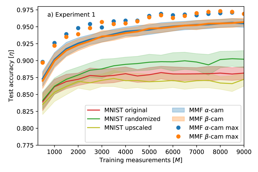
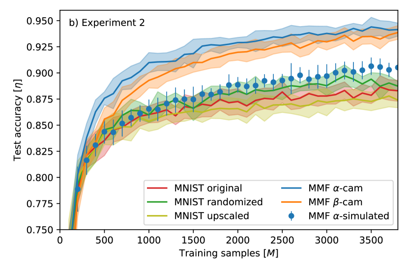
Figure 2: Logistic regression performance using different training datasets. a) Experiment 1, we train the model with up to nine thousand images. The original MNIST set ($l=28$) was used as reference performance (red line) for the logistic regression, together with its upscaled (light green) and randomized (green) versions. Training the classificator with MMF-transformed speckle images (blue and orange curves) exhibited the highest accuracy. We sampled $100$ independent trainings, and we reported with the asterisk plot the best performance obtained with the fiber. b) Experiment 2, we train using up to 3800 images. Compared to panel a), we include also the output of the simulated fiber. The simulation was done by recovering the transmission matrix of the optical element, and using a complex linear transmission model. The simulated model performs better than the MINST set but did not reach the same performance as its experimental counterpart.

Performance of different class of projectors

In experiment 1, we used $10^{4}$ MNIST images, randomly picking up to $9000$ images for training and $1000$ images for testing, using $L=600$. We repeat the parameter optimization for a total of $T=100$ times, varying the number of training samples to test the robustness of our results and analyze statistics. From Fig. 2a, we see how the performances of the MNIST dataset (original, randomized, and upscaled) are similar one to another. The classification problem, in fact, is well known to be a non-linear task, and hardly generalizes using a linear model alone. Instead, using the MMF reservoir higher performances are achieved, approaching 96% test accuracy on average on the largest set used (9000 train examples). We stress that this accuracy is not high in absolute terms since deep neural networks with convolutional layers have been able to reach more than 99% test accuracy on MNIST Lecun et al. (1998), with modern deep architectures raising even up to 99.91% An et al. (2020). However, we are interested in the study of the most simple RC architecture, consisting only of a hardware random-projector layer followed by a linear classifier. With this straightforward setup, the MMF permits to substantially improve the results obtained against a plain linear classifier (88% accuracy with 9000 train examples).

We point out that we did not use the entire MNIST dataset (composed of 60000 images for training and 10000 for testing) but a fraction of it; by increasing the number of training samples, the plot trend in Fig. 2 suggests that there is room for further improvement. Already after $\sim 500$ samplings, the gain provided by the RC approach starts to become evident, and with only 9000 images, we can achieve performance hitting $\sim 97\%$. To achieve the highest accuracy with the experimental data (stars and crosses in the plot of Fig. 2a), we tested several independently initialized optimizations. Interestingly, the performance are independent of the microscopic MMF arrangement, as the two different transmission rules determined by the $\alpha$ and $\beta$ detections perform identically. As a final note, we decided not to tune the hyperparameters of the classifier, so we can expect that their meticulous choice (mainly the $l2$-regularization strength and the stopping threshold) could improve the accuracy curves for all the datasets. In fact, we are not interested in the absolute numbers: our scope is to highlight the improvement determined by the physics of interactions of the MMFs, and the performance gain provided by the fine tuning of the hyperparameters with respect to each dataset would not change the take home message.

The results obtained in experiment 1 are consistent with those of experiment 2. In experiment 2, we take a different static configuration of the fiber in which we alternatively probe the fiber with random and MNIST images. The output using random images was used with the sole scope of estimating the transmission of the fiber using the SmoothGS protocol Ancora et al. (2022). After the recovery of $\mathbb{T}$, we use it to simulate the fiber propagation of the MNIST dataset, obeying to Eq. 2. Interestingly, the simulated speckles does not perform as the experimental data. It still does better than the direct MNIST set, but far from being comparable with the performance obtained with the recorded speckles (Fig. 2b). This reality gap may be due to the presence of noise and other non-linearities that appear experimentally and are not represented in the way we model the physics of the system of Eq. 3 at low power. It might be conjectured that high power non-linearities, also studied in the framework of computational optics with much more intense pulsed light Teğin et al. (2021); Oguz et al. (2022) already contributes at the lower intensities we have been using in our experiments. Compared to the setup used in Teğin et al. (2021), we employed an energy density that is almost three orders of magnitude lower, also determined by the fact that we employed MMFs with large cores of $1mm$. The data acquired by the $\beta$-cam was intentionally strongly underexposed with respect to the $\alpha$-dataset (see the App. .4). By doing so, we notice that substantial thresholding determines a marginally negative impact on the method performance, especially if compared with a better filling of the camera dynamic range in Fig. 2b. On the other hand, we also observe that, even when the camera loses most of the signal, the accuracy of the classifier drops only by a factor of $\sim 2\%$. The weak performance drop possibly supports the idea that the MMF provides random transformations that are particularly robust to carry out classification tasks.

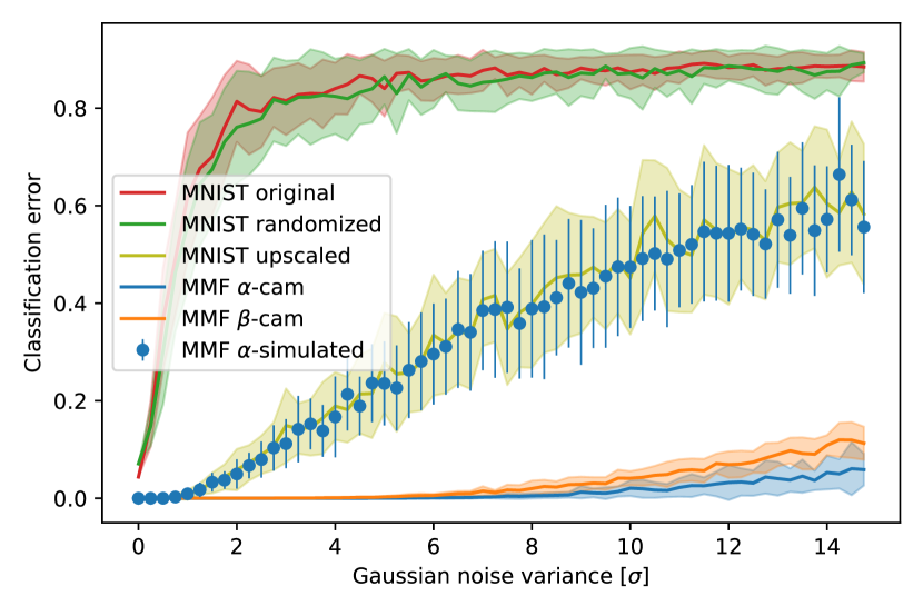
Figure 3: Local energy profiles for models trained on the different projected datasets. Each point corresponds to the train error of configurations sampled with multiplicative noise around the reference, averaged over 30 samples. The reference configurations are models trained on 3800 examples. Error bars show the standard deviation of the error distribution.

Discussion on random projections

With this study we have set a testing ground for different random projectors used to pre-train the MNIST dataset, looking for those enforcing classification. In order to understand why the best accuracy results are obtained with MMFs, we study a measure of the flatness of the energy landscape (i.e., the train error) around the different model solutions. Flatness is supposed to correlate well with generalization properties Baldassi et al. (2022); Jiang et al. (2019); Baldassi et al. (2015, 2016); Chaudhari et al. (2019); Pittorino et al. (2020) and can provide insights into how the geometry of the projected space influences the hardness of the classification problem. We use the method of the local energy to measure the flatness (see Baldassi et al. (2022) and references therein), that consists in adding a multiplicative Gaussian noise to the model parameters, sampling configurations with a given noise, and eventually computing the average classification error (see Appendix section .2 for all the details). Performing this procedure for increasing noise values yields an estimate of the flatness of the reference configuration. In Fig. 3, we see that the local energy profile correlates well with test accuracy shown in Fig. 2: the flattest the solutions, the better the test accuracy (with the exception of the upscaled dataset). A remarkable feature of the local energy profiles of MMF solutions is that they appear stable up to the noise of the order of $10$ times the signal-to-noise ratio. This robustness to noise might be the reason for the excellent generalization performance. This evidence supports the idea that MMFs are promising candidates for reservoir computing. The models trained on MMF-projected data show very low local energy variation. On one hand, this confirms the current idea in the literature that flatness correlates with generalization; and, on the other hand, it raises the question of why MMFs exhibit such a conceptual difference with their idealized model. This reality gap could signal something not yet taken into account in the theoretical description of the physics of experimental set-ups with MMFs.

Influence of the number of modes

xAs a last study, we decided to evaluate the effect of the number of output modes of the reservoir in two different ways. In Fig. 4, we evaluate the effect of downscaling the MMF-output of experiment 2 or cropping it into a smaller window. The effect of these operation is that we variate the size $L$ of the output dataset used to train the classificator and, accordingly, the total number of the output modes $N=L^{2}$. For both camera detections, reducing the number of modes has a negative impact on the performance with the cropping operation being more drastic than rescale. At around $L=400$ pixels, however, both operations had similar effect with performance nearly identical to the full resolution image but with reduced numerical complexity. The fact that the output downscaled by a factor of around $2$ has similar performance to the full resolution dataset seems in agreement with the fact that the spatial correlation of the speckle patter is wider than a single pixel in the detected image, thus introducing redundant information that can be compressed. We report, however, that this also happens with the cropped version of the output, which still shares the same spatial properties of the average speckle size.

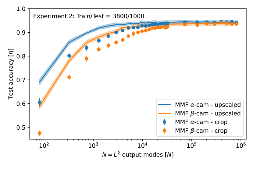
Figure 4: Training accuracy trade-off when reducing the number of output fiber modes in experiment 2. With solid lines, we study the performances obtained using de-magnified camera outputs as a function of their output size. With dots, we report the same study cropping a central window within the speckled image recorded by the camera. For both, we notice that performances remain stable down to a substantial reduction of the number of modes used in the training set (around 400 pixels, 80% less pixel than the full resolution dataset).

IV Perspectives

In this work, we used MMFs to realize random transformations of the MNIST dataset showing that a linear classifier has better accuracy on the MMF-transformed dataset than on the original one. Complementary to high-intensity pulsed excitation Teğin et al. (2021), this transformation (MMF and camera detection) is non-linear even in continuous low-power regime and increases the dimension of the data, but those characteristics are not enough to justify improved accuracy alone. In fact, data upscaling (that increases the dimension), random matrix multiplication (that projects on random space), and the MMF simulation did not reach performances similar to the transformation provided by MMF. As anticipated in section III, our goal was not to compete with the accuracy of more sophisticated architectures, but rather showing that MMFs are simple —yet robust— hardware solutions for optical RC. For example, convolutional neural networks exploit spatial correlations in the data and work particularly well for image datasets. Our approach is, instead, closer to that of a fully connected network, leaving room for applicability to different variety of data types. However, contrarily to general random transformations (that destroy spatial correlations ), the fiber output presents a correlation property determined by the average size of the speckle patterns.

An MMF used as a reservoir is cheap, can flexibly be mounted to deliver light in a user-defined position, and offers a different set of random projections each time it is re-positioned (thus requiring independent training of the output layer). Indeed, we still need an SLM and at least one camera to record the speckled projection, but those are almost unavoidable in any ONNs configuration. To the best of our knowledge, the current state-of-the-art is achieved using FPGA hardware in conjunction with data augmentation, reaching 98% test accuracy Morán et al. (2020). Another approach using disordered optical media exploits polaritons to reach 96% accuracy Mirek et al. (2021), which is comparable with average optimizations obtained with the MMF approach. These results strengthen the fact that MMFs are promising tools for hardware reservoir computing, with the additional advantage of their simplicity and easiness of use. Further, we believe that our results could be relevant for the theoretical understanding of deep neural networks: in the spirit of random-feature models Gerace et al. (2020); Goldt et al. (2022); Baldassi et al. (2022), we showed that the class in which we sample the random features plays important role in the accuracy, as suggested in Perugini and et al. . In fact, while taking a Gaussian random matrix already improves the accuracy a bit, the transformation implemented by an MMF makes a much bigger difference. Further investigation is needed to understand why the specific hardware transformation provided by the MMF is so effective. Here, we put forward some conjectures based on the present study. First, the fact that the accuracy gap between the physical MMF data and its simulation (Fig. 2) is reflected in the local energy profile (Fig. 3) makes us confident that the two approaches indeed belong to different classes of random transformations. The fact the physical MMF transformation is so robust to perturbations is consistent with the great redundancy of the data that emerges from Fig. 4 and Fig. 5, where we see that we can delete the majority of the signal before losing accuracy. We conjecture that the random transformation realized by MMFs leads to well-separated projections in the high-dimensional space that allow for a good classification accuracy that is also resistant to noise, in a way that is reminiscent of error-correcting codes.

.1 Neural network architecture and training procedure

Our classification model involves a fully connected layer that maps linearly the $28\times 28$ image space into a higher dimensional $N=900\times 900$ output space. On the output space, we build a linear classification model using the LogisticRegression function provided by the python library RapidsAi Team (2018), the GPU equivalent of the Scikit-Learn implementation. Given an input pattern $\{\xi_{i}\}_{i=1,..,N}$ the LogisticRegression function performs a weighted average of the $N$ input channels, producing a score $z_{j}=\sum_{i=1}^{N}w_{ji}\xi_{i}$ for each of the $10$ classes corresponding to each type of digit. The scores are then transformed to probabilities with

$$p_{j}=\frac{e^{z_{j}}}{\sum_{j^{\prime}=1}^{10}e^{z_{j}^{\prime}}}$$ (4)

and plugged in a cross-entropy loss function that is a sum of contributions coming from all of the $P$ input patterns that we are using to train the model

$$L(\mathbf{w})=-\sum_{\mu=1}^{P}\log(p_{j^{*}})$$ (5)

where $j^{*}$ is the index of the correct class of each input pattern. The cross-entropy loss $L(\mathbf{w})$ is then minimized with a gradient-descent-related strategy to find the configuration of the weights $\mathbf{w}^{*}$ that has the highest classification accuracy.

.2 Measure of local energy

Given a loss (namely energy) function $L$ that depends on a set of parameters $\mathbf{w}$, we define the local energy as the following expectation value

$$L_{\texttt{local}}(\sigma)=\mathbb{E}_{\eta_{ij}\sim\mathcal{N}(0,\sigma)}L(\{w_{ij}\eta_{ij}\})$$ (6)

where $\{\eta_{ij}\}$ is a set of i.i.d. random Gaussian variables with zero mean and variance $\sigma$ that multiply element-wise the set model parameters $\{w_{ij}\}$. The local energy $L_{\texttt{local}}(\sigma)$ still depends on the variance $\sigma$ of the Gaussian noise. As explained in the main text, we are interested in studying how quickly the local energy increases when we increase $\sigma$: from the literature (see main text) we know that a slower increase is correlated with a higher test accuracy.

.3 Experimental setup

The sketch of the experimental setup is shown in Fig. 1c. In the experiment, we used a continuous Melles Griot he-ne laser ($632.8nm$) as light source. The emitted beam is magnified 15 times through a $5:75cm$ telescope before being imprinted on a Hamamatsu SLM in polarization configuration (model LCOS-SLM x10488 series, pixel size: $20\mu m$). The real space plane of the SLM is then recreated on the entrance facet of the optical fiber using a pair of $50:7.5cm$ focal lenses after the spatially modulated beam profile has been collected. Thorlabs FT-1.0-EMT, $NA=0.39$, $1$ meter long, 1mm core multi-mode optical fiber is the one that has been utilized. We indicate each facet of the MMF with the letter $\alpha$ and $\beta$. Two IDS cameras (UI-5370CP-M-GL and UI-5480CP-M-GL) with pixel sizes of $5.5$ and $2.2\mu m$, respectively, are used to collect the counter-polarized (respect to the laser) reflection from the injection surface as well as the transmission signal. To achieve the same spatial resolution of $1.1\mu m/px$ on both cameras, the magnification was set to $5\times$ and $3\times$ respectively. The MNIST handwritten digits and random masks are alternated in the SLM patterns, which are encoded in $11$-degree gray scale using $28\times 28$ blocks. The random patterns are sent for the sole purpose of the characterization of the fiber transmission, and are not used for training of the classification layer. The light propagating through this disordered optical device reaches both edges and produces a seemingly random interference pattern of intensities (the speckles).

.4 Under-exposure, camera saturation, and measurement stability

When setting the exposure time of the camera, we are implicitly acting on the way it records the signal. If the exposure time is fast enough with respect to the intensity delivered, the camera underexposes the signal, i.e. does not detect the signal in a particular region. The opposite effect, over-exposure, happens when intesity is too high compared to a long exposure of the images. In both cases, a non-linear threshold is introduced in the detected signals. To try to assess its effect on the classifier accuracy, we tried to explore several intensity distributions of the datasets recorded in camera. In experiment 1, Fig. 5a, $\alpha$-cam provides an optimal dynamic range, with low under- (0.1%) and over-exposure (1%). Instead, the $\beta$-cam recorded the signal underexposing 7% of the total pixels in the image. In experiment 2, Fig. 5b, the $\alpha$-cam correctly sample the intensities, whereas $\beta$-cam is set to cut off 37% of the pixels. Additionally, we report also the intensity distribution obtained with the simulation of the light propagating through the fiber and detected by the $\alpha$-cam. We notice a substantial difference between the intensity distribution of the recorded and simulated data: this could explain the different performances achieved by the two datasets.

Over the entire duration of the experiment, we continuously monitored the fiber stability by sending to the SLM an identical image. When the fiber is sufficiently stable, the speckle pattern produced at the facets must be always identical to the ones recorded at the beginning of the experiment. Keeping the camera frame $\tau=0$ as a reference for both $\alpha,\beta$ cameras, we computed the normalized scalar product against the speckle image at a given time $\tau^{\prime}$:

$$\rho\left(\tau,\tau^{\prime}\right)=\frac{s_{\tau}^{\{\alpha,\beta\}}\cdot s_{\tau^{\prime}}^{\{\alpha,\beta\}}}{\left|s_{\tau}^{\{\alpha,\beta\}}\right|^{2}},$$ (7)

where we called $s$ the speckle pattern recorded at the time. Using this metric, $\rho\approx 1$ means the measurements are highly correlated whereas $\rho\approx 0$ implies that the system decorrelated during the measurement. Fig. 6 reports the stability study across the entire duration of the experiment 1. We notice that the $\alpha$-cam remains highly correlated ($96\%$ minimum), compared to the $\beta$-cam (90% minimum). Despite the lower correlation stability and $7\%$ underexposed pixels values, the $\beta$-cam resulted as accurate as the $\alpha$ cam during the classification of the test set (Fig.2).

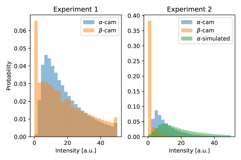
Figure 5: Intensity distribution of the speckle pattern measured in camera $\alpha$ and $\beta$ during two independent experiments. Given a stable laser output, we modify the camera exposure time to force a certain amount of non-linearity (in the form of a recording threshold) in the measuring process. a) In experiment 1, the dynamic range of the camera $\alpha$ fits well the intensity distribution of the speckle images recorded, whereas camera $\beta$ underexposes around $7\%$ of the signal. b) In experiment 2, the camera $\alpha$ have a similar trend to that of experiment 1, but in camera $\beta$ we strongly underexpose the images, cutting out $37\%$ of the light intensity reaching the sensor.

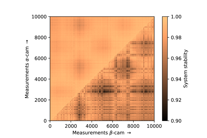
Figure 6: Measurement stability during experiment 1. Keeping the initial probing frame, we compute the normalized scalar product against the output of the same frame at different time for both $\alpha,\beta$ cams. The upper half of the plot is the correlation stability of the $\alpha$-cam (thus how similar the output look when the same input is sent again during the experiment) and the bottom one for $\beta$. In both cases the correlation remained higher than $90\%$.

References

- Hastie et al. (2003) T. Hastie, R. Tibshirani, and M. Wainwright, Statistical Learning with Sparsity, The Lasso and Generalizations (CRC Press, Taylor & Francis Group, 2003).
- MacKay (2003) D. J. MacKay, Information theory, inference and learning algorithms (Cambridge university press, 2003).
- Chizat et al. (2019) L. Chizat, E. Oyallon, and F. Bach, Advances in Neural Information Processing Systems 32 (2019).
- Geiger et al. (2020) M. Geiger, S. Spigler, A. Jacot, and M. Wyart, Journal of Statistical Mechanics: Theory and Experiment 2020, 113301 (2020).
- Gerace et al. (2020) F. Gerace, B. Loureiro, F. Krzakala, M. Mézard, and L. Zdeborová, in International Conference on Machine Learning (PMLR, 2020) pp. 3452–3462.
- Goldt et al. (2022) S. Goldt, B. Loureiro, G. Reeves, F. Krzakala, M. Mézard, and L. Zdeborová, in Mathematical and Scientific Machine Learning (PMLR, 2022) pp. 426–471.
- Baldassi et al. (2022) C. Baldassi, C. Lauditi, E. M. Malatesta, R. Pacelli, G. Perugini, and R. Zecchina, Phys. Rev. E 106, 014116 (2022).
- (8) G. Perugini and et al., (manuscript in preparation).
- Wetzstein et al. (2020) G. Wetzstein, A. Ozcan, S. Gigan, S. Fan, D. Englund, M. Soljačić, C. Denz, D. A. Miller, and D. Psaltis, Nature 588, 39 (2020).
- De Marinis et al. (2019) L. De Marinis, M. Cococcioni, P. Castoldi, and N. Andriolli, IEEE Access 7, 175827 (2019).
- Lin et al. (2018) X. Lin, Y. Rivenson, N. T. Yardimci, M. Veli, Y. Luo, M. Jarrahi, and A. Ozcan, Science 361, 1004 (2018).
- Zhou et al. (2021) T. Zhou, X. Lin, J. Wu, Y. Chen, H. Xie, Y. Li, J. Fan, H. Wu, L. Fang, and Q. Dai, Nature Photonics 15, 367 (2021).
- Li et al. (2021) J. Li, D. Mengu, N. T. Yardimci, Y. Luo, X. Li, M. Veli, Y. Rivenson, M. Jarrahi, and A. Ozcan, Science Advances 7, eabd7690 (2021).
- Abu-Mostafa and Psaltis (1987) Y. S. Abu-Mostafa and D. Psaltis, Scientific American 256, 88 (1987).
- Shen et al. (2017) Y. Shen, N. C. Harris, S. Skirlo, M. Prabhu, T. Baehr-Jones, M. Hochberg, X. Sun, S. Zhao, H. Larochelle, D. Englund, et al., Nature photonics 11, 441 (2017).
- Dong et al. (2019) J. Dong, M. Rafayelyan, F. Krzakala, and S. Gigan, IEEE Journal of Selected Topics in Quantum Electronics 26, 1 (2019).
- Luo et al. (2019) Y. Luo, D. Mengu, N. T. Yardimci, Y. Rivenson, M. Veli, M. Jarrahi, and A. Ozcan, Light: Science & Applications 8, 112 (2019).
- Spall et al. (2022) J. Spall, X. Guo, and A. I. Lvovsky, Optica 9, 803 (2022).
- Zuo et al. (2019) Y. Zuo, B. Li, Y. Zhao, Y. Jiang, Y.-C. Chen, P. Chen, G.-B. Jo, J. Liu, and S. Du, Optica 6, 1132 (2019).
- Wright et al. (2022) L. G. Wright, T. Onodera, M. M. Stein, T. Wang, D. T. Schachter, Z. Hu, and P. L. McMahon, Nature 601, 549 (2022).
- Tanaka et al. (2019) G. Tanaka, T. Yamane, J. B. Héroux, R. Nakane, N. Kanazawa, S. Takeda, H. Numata, D. Nakano, and A. Hirose, Neural Networks 115, 100 (2019).
- Saade et al. (2016) A. Saade, F. Caltagirone, I. Carron, L. Daudet, A. Drémeau, S. Gigan, and F. Krzakala, in 2016 IEEE International Conference on Acoustics, Speech and Signal Processing (ICASSP) (IEEE, 2016) pp. 6215–6219.
- Ballarini et al. (2020) D. Ballarini, A. Gianfrate, R. Panico, A. Opala, S. Ghosh, L. Dominici, V. Ardizzone, M. De Giorgi, G. Lerario, G. Gigli, et al., Nano Letters 20, 3506 (2020).
- Chen et al. (2020) T. Chen, J. van Gelder, B. van de Ven, S. V. Amitonov, B. De Wilde, H.-C. Ruiz Euler, H. Broersma, P. A. Bobbert, F. A. Zwanenburg, and W. G. van der Wiel, Nature 577, 341 (2020).
- Du et al. (2017) C. Du, F. Cai, M. A. Zidan, W. Ma, S. H. Lee, and W. D. Lu, Nature communications 8, 1 (2017).
- Popoff et al. (2010a) S. M. Popoff, G. Lerosey, R. Carminati, M. Fink, A. C. Boccara, and S. Gigan, Physical review letters 104, 100601 (2010a).
- Paudel et al. (2020) U. Paudel, M. Luengo-Kovac, J. Pilawa, T. J. Shaw, and G. C. Valley, Optics express 28, 1225 (2020).
- Porte et al. (2021) X. Porte, A. Skalli, N. Haghighi, S. Reitzenstein, J. A. Lott, and D. Brunner, Journal of Physics: Photonics 3, 024017 (2021).
- Takagi et al. (2017) R. Takagi, R. Horisaki, and J. Tanida, Optical Review 24, 117 (2017).
- Teğin et al. (2021) U. Teğin, M. Yıldırım, İ. Oğuz, C. Moser, and D. Psaltis, Nature Computational Science 1, 542 (2021).
- Ancora and Leuzzi (2022) D. Ancora and L. Leuzzi, Journal of Physics A: Mathematical and Theoretical 55 (2022).
- van Putten and Mosk (2010) E. G. van Putten and A. P. Mosk, Physics 3, 22 (2010).
- Popoff et al. (2010b) S. Popoff, G. Lerosey, M. Fink, and et al., Nat Commun 1, 81 (2010b).
- Aulbach et al. (2011) J. Aulbach, B. Gjonaj, P. M. Johnson, A. P. Mosk, and A. Lagendijk, Phys. Rev. Lett. 106, 103901 (2011).
- Popoff et al. (2014) S. M. Popoff, A. Goetschy, S. F. Liew, A. D. Stone, and H. Cao, Phys. Rev. Lett. 112, 133903 (2014).
- Rotter and Gigan (2017) S. Rotter and S. Gigan, Rev. Mod. Phys. 89, 015005 (2017).
- Drémeau et al. (2015) A. Drémeau, A. Liutkus, D. Martina, O. Katz, C. Schülke, F. Krzakala, S. Gigan, and L. Daudet, Optics express 23, 11898 (2015).
- Huang et al. (2021) G. Huang, D. Wu, J. Luo, L. Lu, F. Li, Y. Shen, and Z. Li, Photonics Research 9, 34 (2021).
- Ancora et al. (2022) D. Ancora, L. Dominici, A. Gianfrate, P. Cazzato, M. De Giorgi, D. Ballarini, D. Sanvitto, and L. Leuzzi, arXiv preprint arXiv:2112.09564 (2022).
- Note (1) The underlined network is one-layer deep because it can be described by a single matrix multiplication as in eq.1.
- Lecun et al. (1998) Y. Lecun, L. Bottou, Y. Bengio, and P. Haffner, Proceedings of the IEEE 86, 2278 (1998).
- An et al. (2020) S. An, M. Lee, S. Park, H. Yang, and J. So, arXiv preprint arXiv:2008.10400 (2020).
- Oguz et al. (2022) I. Oguz, J.-L. Hsieh, N. U. Dinc, U. Teğin, M. Yildirim, C. Gigli, C. Moser, and D. Psaltis, arXiv preprint arXiv:2208.04951 (2022).
- Jiang et al. (2019) Y. Jiang, B. Neyshabur, H. Mobahi, D. Krishnan, and S. Bengio, “Fantastic generalization measures and where to find them,” (2019), arXiv:1912.02178 [cs.LG] .
- Baldassi et al. (2015) C. Baldassi, A. Ingrosso, C. Lucibello, L. Saglietti, and R. Zecchina, Phys. Rev. Lett. 115, 128101 (2015).
- Baldassi et al. (2016) C. Baldassi, C. Borgs, J. T. Chayes, A. Ingrosso, C. Lucibello, L. Saglietti, and R. Zecchina, Proceedings of the National Academy of Sciences 113, E7655 (2016), https://www.pnas.org/content/113/48/E7655.full.pdf .
- Chaudhari et al. (2019) P. Chaudhari, A. Choromanska, S. Soatto, Y. LeCun, C. Baldassi, C. Borgs, J. Chayes, L. Sagun, and R. Zecchina, Journal of Statistical Mechanics: Theory and Experiment 2019, 124018 (2019).
- Pittorino et al. (2020) F. Pittorino, C. Lucibello, C. Feinauer, E. M. Malatesta, G. Perugini, C. Baldassi, M. Negri, E. Demyanenko, and R. Zecchina, arXiv preprint arXiv:2006.07897 2021, 124015 (2020).
- Morán et al. (2020) A. Morán, C. F. Frasser, M. Roca, and J. L. Rosselló, IEEE Transactions on Computers 69, 392 (2020).
- Mirek et al. (2021) R. Mirek, A. Opala, P. Comaron, M. Furman, M. Król, K. Tyszka, B. Seredynski, D. Ballarini, D. Sanvitto, T. C. Liew, et al., Nano letters 21, 3715 (2021).
- Team (2018) R. D. Team, RAPIDS: Collection of Libraries for End to End GPU Data Science (2018).