Oscillations of laminar flow velocity in a channel induced by harmonic perturbation of mass injection velocity through the permeable wall

Abstract

Transient 2D Navier–Stokes equations for the laminar flow of incompressible fluid in a channel with permeable wall are reduced to a single transient one–dimensional equation for the transversal profile of longitudinal flow velocity. Small–amplitude harmonic perturbation of injection velocity induces oscillations of longitudinal velocity with the peak at the walls. The peak amplitude increases with the distance along the channel. The effect of increasing amplitude is explained by formation of linearly growing along the channel perturbation of pressure gradient. With the frequency growth, the peaks move toward to the walls.

I Introduction

Laminar flow of incompressible fluid in channels with permeable wall(s) is of interest for ultrafiltration applications (Chao et al., 2018) and fuel cells (Eikerling and Kulikovsky, 2014). In 1953, Berman (1953) reduced 2D problem for the flow between parallel permeable walls with constant velocity of injection to a single ODE for the transversal shape of longitudinal velocity and provided an elegant asymptotic solution. Later, Berman’s approach has been used to solve the problem of a flow in pipes and ducts with permeable walls and variable along the pipe/duct velocity of suction/injection (Terrill and Thomas (1969); Terrill (1983); Kosinski et al. (1970); Granger et al. (1989); Karode (2001)). So far, however, the transient effects due to time–dependent injection velocity have not been considered.

In 1929, Richardson and Tyler (1929) reported measurements of oscillating flow in a pipe with impermeable wall induced by harmonic longitudinal pressure gradient. They demonstrated formation of a peak of velocity oscillations amplitude close to the pipe wall. A year later, Sexl (1930) developed a model for oscillating flow in a circular pipe and derived a simple solution for the radial shape of velocity amplitude. He showed that the oscillations amplitude is distributed along the radius according to the Bessel function with a peak (shoulder) positioned at the distance

$$l_{*}=\sqrt{\dfrac{\nu}{\omega}}$$ (1)

from the wall. Here $\nu$ is the air kinematic viscosity and $\omega$ is the angular frequency of perturbation. Harris et al. (1969) provided accurate measurements confirming the result of Sexl. In all these works the velocity oscillations were induced by harmonic variation of longitudinal pressure gradient.

Below, unsteady laminar flow of incompressible fluid between parallel walls with a variable and time–dependent rate of mass injection through one of the walls is considered. Following the Berman’s approach, the system of transient Navier–Stokes equations is reduced to a single equation for the transversal shape of longitudinal flow velocity. The equation is used to study the flow response to a small–amplitude harmonic perturbation of the injection velocity. It is shown that such a perturbation induces perturbations of the longitudinal flow velocity. At high frequencies, close to the walls a peak of oscillations amplitude forms which increases dramatically with the distance along the channel. The effect is explained by linearly growing along the channel perturbation amplitude of pressure gradient. The peaks are located at the distance $l_{*}$ from the nearest wall.

II Model

II.1 Basic equations

Consider laminar flow of incompressible fluid between parallel walls separated by the distance $2h$ and let the upper wall be permeable to mass injection (Figure 1).

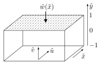
Figure 1: Schematic of the channel. Hatched area indicates the permeable wall through which the mass enters the channel.

Navier–Stokes equations for longitudinal $u$ and transversal $v$ flow velocity components are

$$\dfrac{\partial{u}}{\partial{t}}+u\dfrac{\partial{u}}{\partial{x}}+v\dfrac{\partial{u}}{\partial{y}}=-\dfrac{1}{\rho}\dfrac{\partial{p}}{\partial{x}}+\nu\left(\dfrac{\partial^{2}{u}}{\partial{x}^{2}}+\dfrac{\partial^{2}{u}}{\partial{y}^{2}}\right)$$ (2)

$$\dfrac{\partial{v}}{\partial{t}}+u\dfrac{\partial{v}}{\partial{x}}+v\dfrac{\partial{v}}{\partial{y}}=-\dfrac{1}{\rho}\dfrac{\partial{p}}{\partial{y}}+\nu\left(\dfrac{\partial^{2}{v}}{\partial{x}^{2}}+\dfrac{\partial^{2}{v}}{\partial{y}^{2}}\right)$$ (3)

Here $p$ is the pressure and $\rho$ is the flow density. As $\rho$ is constant, the continuity equation is

$$\dfrac{\partial{u}}{\partial{x}}+\dfrac{\partial{v}}{\partial{y}}=0$$ (4)

Introducing dimensionless variables

$$\tilde{t}=\dfrac{tu_{0}}{h},\quad\tilde{x}=\dfrac{x}{h},\quad\tilde{y}=\dfrac{y}{h},\quad\tilde{u}=\dfrac{u}{u_{0}},\quad\tilde{v}=\dfrac{v}{u_{0}},\\ \tilde{p}=\dfrac{p}{\rho u_{0}^{2}},\quad\tilde{\omega}=\dfrac{\omega h}{u_{0}},$$ (5)

Eqs.(2) – (4) transform to

$$\dfrac{\partial{\tilde{u}}}{\partial{\tilde{t}}}+\tilde{u}\dfrac{\partial{\tilde{u}}}{\partial{\tilde{x}}}+\tilde{v}\dfrac{\partial{\tilde{u}}}{\partial{\tilde{y}}}=-\dfrac{\partial{\tilde{p}}}{\partial{\tilde{x}}}+\dfrac{1}{{\rm Re}}\left(\dfrac{\partial^{2}{\tilde{u}}}{\partial{\tilde{x}}^{2}}+\dfrac{\partial^{2}{\tilde{u}}}{\partial{\tilde{y}}^{2}}\right)$$ (6)

$$\dfrac{\partial{\tilde{v}}}{\partial{\tilde{t}}}+\tilde{u}\dfrac{\partial{\tilde{v}}}{\partial{\tilde{x}}}+\tilde{v}\dfrac{\partial{\tilde{v}}}{\partial{\tilde{y}}}=-\dfrac{\partial{\tilde{p}}}{\partial{\tilde{y}}}+\dfrac{1}{{\rm Re}}\left(\dfrac{\partial^{2}{\tilde{v}}}{\partial{\tilde{x}}^{2}}+\dfrac{\partial^{2}{\tilde{v}}}{\partial{\tilde{y}}^{2}}\right)$$ (7)

$$\dfrac{\partial{\tilde{u}}}{\partial{\tilde{x}}}+\dfrac{\partial{\tilde{v}}}{\partial{\tilde{y}}}=0,$$ (8)

where

$${\rm Re}=\dfrac{u_{0}h}{\nu}$$ (9)

is the inlet Reynolds number, $u_{0}$ is the mean over the $y$–axis $x$–component of inlet flow velocity, and $\omega$ is the angular frequency of perturbations (see below).

Following the idea of Berman (1953) we introduce a stream function

$$\psi=\left(1+\int_{0}^{\tilde{x}}\tilde{w}\left(\tilde{t},\xi\right)\,d\xi\right)f\left(\tilde{t},\tilde{y}\right)$$ (10)

where $\tilde{w}$ is the dimensionless velocity of injection. Setting

$$\tilde{u}=\dfrac{\partial{\psi}}{\partial{\tilde{y}}},\quad\tilde{v}=-\dfrac{\partial{\psi}}{\partial{\tilde{x}}},$$ (11)

Eq.(8) is satisfied. For $\tilde{u}$ and $\tilde{v}$ we thus have

$$\tilde{u}=(1+R)f^{\prime},\quad\tilde{v}=-\tilde{w}f$$ (12)

where

$$R\equiv\int_{0}^{\tilde{x}}\tilde{w}\left(\tilde{t},\xi\right)\,d\xi,$$ (13)

the prime sign indicates partial derivative over $\tilde{y}$ or $\tilde{x}$, depending upon the variable

$$f^{\prime}\equiv\dfrac{\partial{f}}{\partial{\tilde{y}}},\quad\tilde{w}^{\prime}\equiv\dfrac{\partial{\tilde{w}}}{\partial{\tilde{x}}},$$ (14)

and similar for higher derivatives. Substituting Eqs.(12) into Eqs.(6), (7) we come to

$$\dfrac{\partial{(1+R)f^{\prime}}}{\partial{\tilde{t}}}+(1+R)\tilde{w}\left(f^{\prime}f^{\prime}-ff^{\prime\prime}\right)\\ =-\dfrac{\partial{\tilde{p}}}{\partial{\tilde{x}}}+\dfrac{1}{{\rm Re}}\left(\tilde{w}^{\prime}f^{\prime}+(1+R)f^{\prime\prime\prime}\right)$$ (15)

$$-\dfrac{\partial{(\tilde{w}f)}}{\partial{\tilde{t}}}+\left(\tilde{w}^{2}-(1+R)\tilde{w}^{\prime}\right)ff^{\prime}\\ =-\dfrac{\partial{\tilde{p}}}{\partial{\tilde{y}}}-\dfrac{1}{{\rm Re}}\left(\tilde{w}^{\prime\prime}f+\tilde{w}f^{\prime\prime}\right)$$ (16)

Differentiating Eq.(15) over $\tilde{y}$ and Eq.(16) over $\tilde{x}$ we get

$$\dfrac{\partial{(1+R)f^{\prime\prime}}}{\partial{\tilde{t}}}+(1+R)\tilde{w}\left(f^{\prime}f^{\prime\prime}-ff^{\prime\prime\prime}\right)\\ =-\dfrac{\partial{}}{\partial{\tilde{y}}}\left(\dfrac{\partial{\tilde{p}}}{\partial{\tilde{x}}}\right)+\dfrac{1}{{\rm Re}}\bigl{(}\tilde{w}^{\prime}f^{\prime\prime}+(1+R)f^{\prime\prime\prime\prime}\bigr{)}$$ (17)

$$-\dfrac{\partial{(\tilde{w}^{\prime}f)}}{\partial{\tilde{t}}}+\bigl{(}\tilde{w}\tilde{w}^{\prime}-(1+R)\tilde{w}^{\prime\prime}\bigr{)}ff^{\prime}\\ =-\dfrac{\partial{}}{\partial{\tilde{x}}}\left(\dfrac{\partial{\tilde{p}}}{\partial{\tilde{y}}}\right)-\dfrac{1}{{\rm Re}}\left(\tilde{w}^{\prime\prime\prime}f+\tilde{w}^{\prime}f^{\prime\prime}\right)$$ (18)

Subtracting Eq.(18) from Eq.(17) we come to

$$\dfrac{\partial{}}{\partial{\tilde{t}}}\biggl{(}(1+R)f^{\prime\prime}+\tilde{w}^{\prime}f\biggr{)}+(1+R)\tilde{w}\left(f^{\prime}f^{\prime\prime}-ff^{\prime\prime\prime}\right)\\ -\bigl{(}\tilde{w}\tilde{w}^{\prime}-(1+R)\tilde{w}^{\prime\prime}\bigr{)}ff^{\prime}\\ =\dfrac{1}{{\rm Re}}\bigl{(}2\tilde{w}^{\prime}f^{\prime\prime}+(1+R)f^{\prime\prime\prime\prime}+\tilde{w}^{\prime\prime\prime}f\bigr{)}$$ (19)

Eq.(19) is the general equation for the flow in channel with a non–uniform along $\tilde{x}$ and time–dependent velocity of mass injection. The boundary conditions for this equation follow from Eqs.(12):

$$f(1)=1,\quad f^{\prime}(1)=0,\quad f(-1)=f^{\prime}(-1)=0$$ (20)

II.2 Small oscillations of uniform injection velocity

It is advisable to consider the case of uniform along $\tilde{x}$ injection velocity $\tilde{w}$. Setting in Eq.(19) $R=\tilde{w}(\tilde{t})\,\tilde{x}$ and chalking out the terms with $\tilde{w}^{\prime}$, $\tilde{w}^{\prime\prime}$, and $\tilde{w}^{\prime\prime\prime}$, we arrive at

$$\left(\dfrac{\tilde{x}}{1+\tilde{x}\tilde{w}}\right)\dfrac{\partial{\tilde{w}}}{\partial{\tilde{t}}}f^{\prime\prime}+\dfrac{\partial{f^{\prime\prime}}}{\partial{\tilde{t}}}+\tilde{w}\bigl{(}f^{\prime}f^{\prime\prime}-ff^{\prime\prime\prime}\bigr{)}=\dfrac{f^{\prime\prime\prime\prime}}{{\rm Re}}$$ (21)

Eq.(21) can be integrated over $\tilde{y}$ once, leading to

$$\left(\dfrac{\tilde{x}}{1+\tilde{x}\tilde{w}}\right)\dfrac{\partial{\tilde{w}}}{\partial{\tilde{t}}}f^{\prime}+\dfrac{\partial{f^{\prime}}}{\partial{\tilde{t}}}+\tilde{w}\bigl{(}f^{\prime}f^{\prime}-ff^{\prime\prime}\bigr{)}-\dfrac{f^{\prime\prime\prime}}{{\rm Re}}=k$$ (22)

where $k$ is determined from solution of Eq.(22) with four boundary conditions, Eq.(20). Eq.(22) is the transient version of equation derived by Berman (1953).

Substituting

$$\begin{split}&\tilde{w}=\tilde{w}_{0}+\tilde{w}_{1}(\tilde{\omega})\exp({\rm i}\tilde{\omega}\tilde{t}),\quad|\tilde{w}_{1}|\ll|\tilde{w}_{0}|\\ &f=f_{0}(\tilde{y})+f_{1}(\tilde{\omega},\tilde{y})\exp({\rm i}\tilde{\omega}\tilde{t}),\quad|f_{1}|\ll|f_{0}|\\ &k=k_{0}+k_{1}\end{split}$$ (23)

into Eq.(22), neglecting terms with the perturbation products and subtracting the static equation Eq.(25), we come to a linear problem for the complex perturbation amplitude $f_{1}(\tilde{\omega},\tilde{y})$:

$${\rm i}\tilde{\omega}\left(\dfrac{\tilde{x}\tilde{w}_{1}f_{0}^{\prime}}{1+\tilde{x}\tilde{w}_{0}}+f_{1}^{\prime}\right)+\tilde{w}_{0}\bigl{(}2f_{0}^{\prime}f_{1}^{\prime}-f_{0}f_{1}^{\prime\prime}-f_{0}^{\prime\prime}f_{1}\bigr{)}\\ +\tilde{w}_{1}\bigl{(}f_{0}^{\prime}f_{0}^{\prime}-f_{0}f_{0}^{\prime\prime}\bigr{)}-\dfrac{f_{1}^{\prime\prime\prime}}{{\rm Re}}=k_{1}$$ (24)

where $f_{0}(\tilde{y})$ is a solution to the static Berman’s equation

$$\tilde{w}_{0}\left(f_{0}^{\prime}f_{0}^{\prime}-f_{0}f_{0}^{\prime\prime}\right)-\dfrac{f_{0}^{\prime\prime\prime}}{{\rm Re}}=k_{0}$$ (25)

Here, the subscripts 0 and 1 mark the static variables and the small perturbation amplitudes in the $\omega$–space, respectively.

The boundary condition for $f_{1}$ at $\tilde{y}=1$ follows from equation $\tilde{v}_{0}+\tilde{v}_{1}=-(\tilde{w}_{0}+\tilde{w}_{1})(f_{0}+f_{1})$. At the upper wall, $\tilde{v}_{1}=-\tilde{w}_{1}$; neglecting the product $\tilde{w}_{1}f_{1}$ and taking into account that $\tilde{v}_{0}=-\tilde{w}_{0}f_{0}$, $f_{0}(1)=1$, we get $f_{1}(1)=0$. Thus, the boundary conditions for Eq.(24) are

$$f_{1}(1)=f_{1}^{\prime}(1)=f_{1}(-1)=f_{1}^{\prime}(-1)=0.$$ (26)

III Results and Discussion

The spectrum of $f_{1}^{\prime}$ at the mid–plane $\tilde{y}=0$ and $\tilde{x}=100$ for the parameters in Table 1 resembles Warburg finite–length transport impedance (Warburg, 1899) (Figure 2). Since $\tilde{u}_{1}\sim f_{1}^{\prime}$, Eq.(12), of particular interest is the shape of $\operatorname{Re}\left(f_{1}^{\prime}\right)$ representing the longitudinal velocity oscillations in–phase with the applied perturbation. Eq.(24) contains a term explicitly depending on $\tilde{x}$; thus, this shape changes with $\tilde{x}$ and with the frequency. Evolution of this shape at $\tilde{x}=1$ with the growth of frequency is depicted in Figure 3a. With the frequency growth, two “shoulders” at the walls and a valley between them form (the curve for $10^{2}$ Hz, Figure 3a). The amplitude of oscillation in the valley is negative meaning that here, the oscillations decelerate the flow. Upon further frequency growth, the shoulders move toward the walls (solid line in Figure 3a). The asymmetry of the curves is due to mass injection at the upper wall.

Channel depth $2h$, m	$0.1\cdot 10^{-2}$
Channel length $L$, m	1.0
Air density, $\rho$, kg m-3	1.06
Air kinematic viscosity, $\nu$, m2 s-1	$1.886\cdot 10^{-5}$
Inlet flow velocity $u_{0}$, m s-1	10
Reynolds number ${\rm Re}$	530
Injection velocity $w$, m s-1	0.1

Table 1: The flow parameters for the calculations.

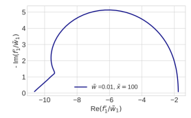
Figure 2: Nyquist spectrum of the longitudinal velocity oscillations amplitude $f_{1}^{\prime}/\tilde{w}_{1}$ at the mid–plane $\tilde{y}=0$ and $\tilde{x}=100$ (one tenths of the channel length).

At $\tilde{x}=1$, the oscillations amplitude in the shoulders is on the order of unity, i.e., the relative amplitude of velocity oscillations is of the same order of magnitude as the applied amplitude of injection velocity oscillations. However, the longitudinal velocity is two orders of magnitude larger than the injection velocity (Table 1), meaning that the system works as a hydrodynamic “amplifier”. A close analogy is a field–effect transistor, in which a small variation of gate potential induces large variation of the source–drain current.

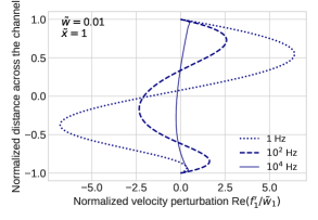
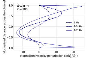
Figure 3: Transversal shape of longitudinal flow velocity oscillations amplitude for the indicated frequencies at (a) $\tilde{x}=1$ and (b) $\tilde{x}=100$ (one tenths of the channel length).

The most interesting effect is dramatic growth of the shoulders with the distance along the channel (Figure 3b). Formally, the effect can be rationalized considering the problem for the flow with zero static injection velocity, however, excited periodically at the permeable wall (excited Poiseuille flow). An equation for the flow velocity spectrum is obtained setting $\tilde{w}_{0}=0$ in Eq.(24). Further, at large frequencies, the term $\tilde{w}_{1}\bigl{(}f_{0}^{\prime}f_{0}^{\prime}-f_{0}f_{0}^{\prime\prime}\bigr{)}$ in Eq.(24) can be neglected, and we come to

$${\rm i}\tilde{\omega}\bigl{(}\tilde{x}\tilde{w}_{1}f_{0}^{\prime}+f_{1}^{\prime}\bigr{)}-\dfrac{f_{1}^{\prime\prime\prime}}{{\rm Re}}=k_{1}$$ (27)

For Poiseuille flow, $f_{0}^{\prime}=3(1-\tilde{y}^{2})/4$ and solution to Eqs.(27), (26) leads to

$$f_{1}^{\prime}=\dfrac{\tilde{x}\tilde{w}_{1}}{4}\left(3\tilde{y}^{2}-1-\dfrac{2\bigl{(}\phi\cosh(\phi\tilde{y})-\sinh(\phi)\bigr{)}}{\phi\cosh(\phi)-\sinh(\phi)}\right),\\ \phi=\sqrt{{\rm i}\tilde{\omega}{\rm Re}}$$ (28)

Eq.(28) shows that the longitudinal velocity perturbation amplitude is proportional to the distance $\tilde{x}$. The numerical transversal ($\tilde{y}$–) dependence of the perturbation amplitude for the three frequencies is shown in Figure 4. The curves are symmetric with respect to the mid–plane; nonetheless, the trend with the frequency growth is the same as in Figure 3: a shape with the two shoulders forms (Figure 4). Note that the shoulders in Figure 4 are twice larger than those in Figure 3b, i.e., zero injection velocity enhances the effect. Points in Figure 4 show the analytical solution, Eq.(28).

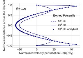
Figure 4: Transversal shape of longitudinal flow velocity oscillations amplitude for the transient Poiseuille problem, Eq.(27). Points show the analytical solution, Eq.(28).

At large frequencies, the term with hyperbolic functions in Eq.(28) has a sharp peak in a narrow domain near the walls, at $1-|y|\lesssim\epsilon$. The dimensionless width $\epsilon$ of this domain is on the order of $1/|\phi|=1/\sqrt{\tilde{\omega}{\rm Re}}$, which in the dimension form gives the distance between the shoulder and the wall, Eq.(1).

To understand the physics behind enhancement of velocity oscillations amplitude along the channel, consider equation (15) for the pressure gradient. Setting $R=\tilde{w}\tilde{x}$, neglecting the term with $\tilde{w}^{\prime}$ and performing linearization and Fourier–transform, we come to

$$-\dfrac{\partial{\tilde{p}_{1}}}{\partial{\tilde{x}}}={\rm i}\tilde{\omega}\bigl{(}(1+\tilde{x}\tilde{w}_{0})f_{1}^{\prime}+\tilde{x}\tilde{w}_{1}f_{0}^{\prime}\bigr{)}\\ +\tilde{w}_{1}\left(1+2\tilde{x}\tilde{w}_{0}\right)\left(f_{0}^{\prime}f_{0}^{\prime}-f_{0}f_{0}^{\prime\prime}\right)\\ +(1+\tilde{x}\tilde{w}_{0})\tilde{w}_{0}\left(2f_{0}^{\prime}f_{1}^{\prime}-f_{1}f_{0}^{\prime\prime}-f_{0}f_{1}^{\prime\prime}\right)\\ -\dfrac{1}{{\rm Re}}\left((1+\tilde{x}\tilde{w}_{0})f_{1}^{\prime\prime\prime}+\tilde{x}\tilde{w}_{1}f_{0}^{\prime\prime\prime}\right)$$ (29)

where $\tilde{p}=\tilde{p}_{0}(\tilde{x},\tilde{y})+\tilde{p}_{1}(\tilde{\omega},\tilde{x},\tilde{y})\exp({\rm i}\tilde{\omega}\tilde{t})$ has been substituted.

With the parameters from Table 1, the average over $\tilde{y}$–axis real part of normalized pressure gradient perturbation

$$-\dfrac{1}{\tilde{w}_{1}}\Braket{\dfrac{\partial{\tilde{p}_{1}}}{\partial{\tilde{x}}}}\equiv-\dfrac{1}{2\tilde{w}_{1}}\int_{-1}^{1}\dfrac{\partial{\tilde{p}_{1}}}{\partial{\tilde{x}}}\,d\tilde{y}$$ (30)

increases linearly along the channel (Figure 5). This explains the growth of oscillation amplitude with $\tilde{x}$. Indeed, the Sexl model (Sexl, 1930) for perturbed flow in the channel with impermeable walls results in the velocity oscillations amplitude proportional to the amplitude of pressure gradient perturbation. In the channel with mass injection, a linearly increasing perturbation of pressure gradient forms, leading to growing amplitude of velocity oscillations.

This result can be shown directly. From the first of Eqs.(12) we can write

$$\tilde{u}_{0}+\tilde{u}_{1}=(1+R_{0}+R_{1})(f^{\prime}_{0}+f^{\prime}_{1})\\ \simeq(1+R_{0})f^{\prime}_{0}+(1+R_{0})f^{\prime}_{1}+R_{1}f^{\prime}_{0}$$ (31)

Since $\tilde{u}_{0}=(1+R_{0})f^{\prime}_{0}$, from Eq.(31) we find

$$\tilde{u}_{1}=(1+R_{0})f^{\prime}_{1}+R_{1}f^{\prime}_{0}$$ (32)

Integrating the last equation over $\tilde{y}\in[-1,1]$ and taking into account the boundary conditions (20), (26), we find $\Braket{\tilde{u}_{1}}=R_{1}/2$. In terms of perturbation amplitudes the last equation reads

$$\Braket{\tilde{u}_{1}}=\dfrac{\tilde{w}_{1}\tilde{x}}{2},$$ (33)

i.e., the amplitude of average longitudinal flow velocity oscillations is independent of frequency and it increases linearly with $\tilde{x}$.

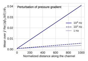
Figure 5: The real component of pressure gradient perturbation amplitude along the channel. Perturbation amplitude of injection velocity is $10^{-3}$ m s^-1.

Finally, we note that at finite $\tilde{w}_{0}$, the shoulders in Figure 3 grow with $\tilde{x}$ as long as $\tilde{x}\tilde{w}_{0}$ is small, as Eq.(24) shows. In long channels, for $\tilde{x}\tilde{w}_{0}\gg 1$ the dependence of Eq.(24) on $\tilde{x}$ vanishes and the shoulders amplitude saturates. This dependence, however, retains in the general case of variable with $\tilde{x}$ injection velocity.

IV Conclusions

A transient model of laminar incompressible flow between parallel walls, one of which is permeable to mass injection is developed. Two–dimensional transient Navier–Stokes equations and continuity equation are reduced to a single one–dimensional transient equation for the longitudinal velocity. Linearization and Fourier–transform lead to equation for the small perturbation amplitude of this velocity.

The results show that a small harmonic perturbation of injection velocity at the permeable wall is converted to oscillations of longitudinal flow velocity. At high frequencies, the transversal profile of oscillations amplitude exhibits two peaks which dramatically increase along the channel. The effect is caused by linearly growing along the channel perturbation amplitude of pressure gradient. The peaks are located at the distance $\sqrt{\nu/\omega}$ from the walls, i.e., with the frequency growth each peak moves toward the nearest wall.

Conflict of interest statement

The author declares no conflict of interest.

References

• Chao et al. (2018) G. Chao, Y. Shuili, S. Yufei, G. Zhengyang, Y. Wangzhen, and R. Liumo. A review of ultrafiltration and forward osmosis: Application and modification. IOP Conference Series: Earth and Environmental Science, 128:012150, Mar 2018. doi: 10.1088/1755-1315/128/1/012150.
• Eikerling and Kulikovsky (2014) M. Eikerling and A. A. Kulikovsky. Polymer Electrolyte Fuel Cells: Physical Principles of Materials and Operation. CRC Press, London, 2014.
• Berman (1953) A. S. Berman. Laminar flow in channels with porous walls. J. Appl. Phys., 24:1232–1235, 1953. doi: 10.1063/1.1721476.
• Terrill and Thomas (1969) R. M. Terrill and P. W. Thomas. On laminar flow through a uniformly porous pipe. Appl. Sci. Res., 21:37–67, 1969. doi: 10.1007/BF00411596.
• Terrill (1983) R. M. Terrill. Laminar flow in a porous tube. J. Fluids Eng., 105:303–307, 1983. doi: 10.1115/1.3240992.
• Kosinski et al. (1970) A. A. Kosinski, F. P. Schmidt, and E. N. Lightfoot. Velocity profiles in porous-walled ducts. Ind. Eng. Chem. Fundam., 9:502–505, 1970. doi: 10.1021/i160035a033.
• Granger et al. (1989) J. Granger, J. Dodds, and N. Midoux. Laminar flow in channels with porous walls. Chem. Eng. J., 42:193–204, 1989. doi: 10.1016/0300-9467(89)80087-5.
• Karode (2001) S. K. Karode. Laminar flow in channels with porous walls, revisited. J. Membr. Sci., 191:237–241, 2001. doi: 10.1016/S0376-7388(01)00546-4.
• Richardson and Tyler (1929) E. G. Richardson and E. Tyler. The transverse velocity gradient near the mouths of pipes in which an alternating or continuous flow of air is established. Proc. Phys. Soc., 42:1–15, 1929. doi: 10.1088/0959-5309/42/1/302.
• Sexl (1930) T Sexl. Über den von E. G. Richardson entdeckten Annulareffekt. Z. Phys., 61:349–362, 1930. doi: 10.1007/BF01340631.
• Harris et al. (1969) J. Harris, G. Peevt, and W. L. Wilkinson. Velocity profiles in laminar oscillatory flow in tubes. J. Phys. E: Sci. Instrum., 2:913–916, 1969. doi: 10.1088/0022-3735/2/11/301.
• Warburg (1899) E. Warburg. Über das Verhalten sogenannter unpolarisirbarer Electroden gegen Wechselstrom. Ann. Physik und Chemie, 67:493–499, 1899. doi: 10.1002/andp.18993030302.