The Gaia-ESO Survey: Lithium measurements
and new curves of growth^,

Abstract

Context. The Gaia-ESO Survey (GES) is a large public spectroscopic survey that was carried out using the multi-object FLAMES spectrograph at the Very Large Telescope. The survey provides accurate radial velocities, stellar parameters, and elemental abundances for $\sim$ 115 000 stars in all Milky Way components.

Aims. In this paper we describe the method adopted in the final data release to derive lithium equivalent widths (EWs) and abundances.

Methods. Lithium EWs were measured using two different approaches for FGK and M-type stars, to account for the intrinsic differences in the spectra. For FGK stars, we fitted the lithium line using Gaussian components, while direct integration over a predefined interval was adopted for M-type stars. Care was taken to ensure continuity between the two regimes. Abundances were derived using a new set of homogeneous curves of growth that were derived specifically for GES, and which were measured on a synthetic spectral grid consistently with the way the EWs were measured. The derived abundances were validated by comparison with those measured by other analysis groups using different methods.

Results. Lithium EWs were measured for $\sim$ 40 000 stars, and abundances could be derived for $\sim$ 38 000 of them. The vast majority of the measures (80%) have been obtained for stars in open cluster fields. The remaining objects are stars in globular clusters, or field stars in the Milky Way disc, bulge, and halo.

Conclusions. The GES dataset of homogeneous lithium abundances described here will be valuable for our understanding of several processes, from stellar evolution and internal mixing in stars at different evolutionary stages to Galactic evolution.

1 Introduction

Lithium is a key element for our understanding of several open issues in astrophysics, from Big-Bang nucleosynthesis to the chemical evolution of the Milky Way, to mixing processes in stellar interiors and stellar evolution (e.g. Randich & Magrini, 2021, and references therein). Precise and homogeneous measures for large samples of stars are fundamental to address these issues.

The Gaia-ESO Survey (hereafter GES; Gilmore et al., 2012; Randich et al., 2013) is a large public spectroscopic survey that observed $\sim$ $10^{5}$ stars in all Milky Way components, from the thin and thick disc to the bulge and halo, including 65 (science and calibration) open clusters and 15 globular clusters. The GES spectra were acquired with the Fiber Large Array Multi-Element Spectrograph (FLAMES; Pasquini et al., 2002) mounted on the UT2 unit of the Very Large Telescope, using the high-resolution Ultraviolet and Visual Echelle Spectrograph (UVES) and the Giraffe instrument operated in MEDUSA mode. The dataset was complemented with additional spectra of stars in open and globular clusters retrieved from the ESO archive and observed with the same setups, increasing the total number of open clusters to 83. The final dataset provides precise radial velocities and homogeneous stellar parameters and chemical abundances of up to 31 elements, including lithium, for $\sim$ 115 000 stars.

A detailed overview of the survey goals and strategy, and of the data analysis is provided by Gilmore et al. (2022) and Randich et al. (2022). More specific papers describe the target selection (Stonkutė et al., 2016; Bragaglia et al., 2022), the calibration strategy (Pancino et al., 2017), the data reduction pipelines, and the derivation of radial and rotational velocities (Sacco et al., 2014; Jeffries et al., 2014; Jackson et al., 2015). Spectral analysis of late-type stars was performed by different analysis nodes within each of the three dedicated working groups: WG10 and WG11 for FGK stars observed with Giraffe and UVES, respectively, and WG12 for pre-main-sequence (PMS) stars (Smiljanic et al., 2014; Lanzafame et al., 2015, Worley et al. in prep.). The individual results were then homogenised and combined to produce the final recommended values. The analysis was performed in two steps: first, atmospheric parameters were derived and homogenised, then chemical abundances were obtained using the recommended atmospheric parameters as input.

In this paper we describe the derivation of lithium abundances for the Sixth internal Data Release (iDR6), which corresponds to the final data release published in the ESO archive. In iDR6, recommended lithium abundances were only derived by the Arcetri node. This approach differs from previous data releases, where a multi-node analysis was performed just as for the other parameters and abundances (see Smiljanic et al., 2014; Lanzafame et al., 2015). Because of the peculiarity of lithium, which is measured by a single line and depends on stellar mass and age, and of the different subsets of spectra that the individual nodes were able to analyse, the homogenisation of the results obtained from different nodes did not prove to be efficient in providing sufficiently homogeneous results. However, a sub-sample of the spectra was still analysed by other nodes, and these measurements were used for validation purposes.

The method adopted by the Arcetri node is based on the measurement of equivalent widths (EWs) and the use of curves of growth (COGs) to derive the abundances. The advantage of the EW method over spectral synthesis is that EWs can also be measured for spectra where spectral synthesis is not feasible, or when not all atmospheric parameters can be derived (e.g. for low signal-to-noise spectra, or young rapidly rotating stars). However, to ensure that no bias is introduced, it is preferable that both EWs and COGs are derived in a consistent way. For this reason, a new set of COGs, specific for GES, was also derived.

The paper is organised as follows. In Sect. 2 we present the lithium data available in GES. The derivation of the new set of COGs and the lithium measurements are described in Sects. 3 and 4, respectively. In Sect. 5 we discuss the validation of the results. The final catalogue is presented in Sect. 6, and caveats for the measures are given in Sect. 7. A summary is provided in Sect. 8.

2 Lithium in GES

Lithium can be measured from the Li i doublet at 6707.8 Å, which is available in GES spectra acquired with the UVES U580 setup (480–680 nm, $R=47\,000$) and with the Giraffe HR15N grating (644–680 nm, $R\sim$ 17 000). The UVES U580 setup was used for FGK turn-off and giant stars in old open clusters, globular clusters, and the Milky Way fields, and for the brightest main-sequence stars in young open clusters. Giraffe HR15N spectra were acquired for FGK stars on the main sequence in open and globular clusters, and for G- to M-type PMS stars in young open clusters. A fraction of the targets was observed with both instruments for cross-calibration purposes (see Bragaglia et al., 2022).

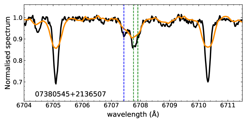
Figure 1: UVES (black, S/N=119) and Giraffe (orange, S/N=223) spectra of the giant star 07380545+2136507 which was observed with both instruments. The vertical green and blue dashed lines mark the positions of the lithium doublet and of the 6707.4 Å iron line, respectively.

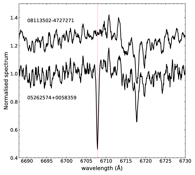
Figure 2: Spectra of two M-type dwarf stars with $T_{\mathrm{eff}}\sim 3500$ K and solar metallicity observed with Giraffe. The upper and lower spectrum correspond to a fully depleted star ($A(\mathrm{Li})<-1.0$) and to a star with $A$(Li) $\sim$ 2.0, respectively. The spectra are normalised to their average flux and the upper one has been arbitrarily shifted upwards by 0.25 for clarity. The vertical red dotted line marks the mean position of the lithium line.

The large variety of the stellar samples targeted by GES makes a homogeneous determination of lithium abundances challenging. In the case of FGK stars, the lithium line is blended mainly with the nearby Fe i line at 6707.43 Å, plus a few weaker components from other elements. At the UVES resolution, it is generally possible to deblend the lines and measure directly the lithium-only EW, EW(Li). Exceptions to this are stars with high rotation rates ($v\sin i\ga 30$ km s^-1), or young stars with very strong lithium, where the deblending might not be possible. The deblending is never possible for Giraffe HR15N spectra. In such cases, only the total EW(Li+Fe) can be measured. An example of this is shown in Fig. 1, where we compare the spectra of a giant star observed with both instruments: while in UVES the iron and lithium lines, although partially overlapping, are clearly distinct, this is not the case for Giraffe.

In M-type stars, the measurement of lithium abundances is complicated by the presence of molecular bands and additional lines from other elements, which are severely blended with lithium and cause a strongly depressed pseudo-continuum (e.g. Zapatero Osorio et al., 2002). The pseudo-continuum trend can be clearly seen in Fig. 2, where we compare the spectrum of an M-type star with lithium abundance $A$(Li) $\sim$ 2.0, with that of a fully depleted star with similar temperature and rotation; the wide depression around the lithium position caused by the other line blends is clearly evident in the latter. This pseudo-continuum masks the position of the real continuum level, preventing the measure of the true lithium EW, contrary to what can be done in hotter stars. In this case, only a pseudo-EW (pEW) can be derived.

The above considerations imply that different approaches must be adopted to measure lithium in FGK- and M-type stars. However, the chosen method must ensure the highest possible consistency between the measures of the two sets of stars, minimising any discontinuity between the two regimes. To this aim, we developed a specific code based on python to measure EWs and pEWs and the corresponding COGs in a consistent way.

3 New lithium curves of growth

The need for a new set of homogeneous COGs for lithium arises from the fact that COGs covering the entire range of atmospheric parameters of GES spectra are not available in the literature. As mentioned by Lanzafame et al. (2015), in previous data releases we used the COGs derived by Soderblom et al. (1993) for $T_{\mathrm{eff}}=4000-6500$ K, and those by Palla et al. (2007) for $T_{\mathrm{eff}}\leq 4000$ K. However, these COGs are only valid for dwarfs, therefore they are not applicable to giants; they were computed for solar metallicity and are therefore not valid for more metal-poor or metal-rich stars; and they were derived using inconsistent methods, causing discontinuity problems around 4000 K. Moreover, literature COGs were derived using different sets of model atmospheres, which are not necessarily the same used in GES.

To derive the new set of COGs, we used a grid of synthetic spectra that was computed as in de Laverny et al. (2012) and Guiglion et al. (2016), within the context of the AMBRE project (de Laverny et al., 2013). The grid is based on the same model atmospheres used in GES, namely the one-dimensional MARCS models in local thermodynamic equilibrium (LTE; Gustafsson et al., 2008), and was computed assuming standard [$\alpha$/Fe] ratios. The parameters were chosen to cover the entire range of late-type stars observed in GES, namely $3000\leq T_{\mathrm{eff}}\leq 8000$ K, $0.5\leq\log g\leq 5.0$ and $-2.50\leq\mathrm{[Fe/H]}\leq+0.50$. Lithium abundances vary from $A(\mathrm{Li})=-1.0$ to $A(\mathrm{Li})=+4.0$ in steps of 0.2 dex, except for $\mathrm{[Fe/H]}<-1.50$, where abundances have been limited to $A(\mathrm{Li})\leq+3.4$, since higher abundances at such low metallicities are extremely rare (e.g. Sanna et al., 2020).

As mentioned in the previous section, the differences in the spectra of FGK and M-type stars require the adoption of two different approaches to measure the EWs. For this reason, two separate sets of COGs were derived, one for FGK stars, covering the temperature range 4000 K$\,\leq T_{\mathrm{eff}}\leq 8000$ K, and a separate set for M-type stars, covering the range 3000 K$\,\leq T_{\mathrm{eff}}\leq 4500$ K. The two sets overlap over the range $4000-4500$ K to ensure continuity. The M-type COGs were however limited to [Fe/H] $\geq-1.5$, since lower-metallicity M-type stars are generally not present in GES.

3.1 FGK stars

In the case of FGK stars, which were observed with both UVES and Giraffe, we need a set of COGs that can equally be applied to cases where we can directly measure the deblended lithium line and to those where only the blended line can be measured. To achieve this, COGs were derived for the lithium component only, and a corresponding set of corrections for the Fe blend was computed. These corrections can be applied to derive the Li-only EW when only the total EW(Li+Fe) can be measured, before computing the abundances.

The EWs of the lithium doublet and of the Fe blend were measured on the spectral grid degraded to the UVES resolution, down to $T_{\mathrm{eff}}=4000$ K. For simplicity, and to ease the deblending of the two components, for each set of atmospheric parameters both Li and Fe EWs were simultaneously measured only on the spectrum with $A(\mathrm{Li})=-1.0$, which was used as reference spectrum. The lines were fitted with Gaussian components, assuming a local linear continuum, using the code described in Sect. 4.2. The EWs of the Fe blend obtained from this fit were taken as the blend correction for the corresponding parameters. For higher lithium abundances, the lithium EW was measured by spectral subtraction, that is, we subtracted the reference spectrum from the corresponding spectra with $A(\mathrm{Li})>-1.0$, and integrated the resulting residual components. We chose to integrate the residuals, instead of fitting them, because at the highest lithium abundances the adopted Gaussian components are not able to fit the residual line correctly, especially below 4500 K, where the lithium line develops significant wings and is better described by a Voigt profile. The half-width of the integration interval was set to $d=3.5\sigma$, where $\sigma$ is the width of the corresponding best-fit Gaussian, with a maximum allowed value of 0.8 Å. The latter value corresponds to the typical width of the core of the line for $A(\mathrm{Li})>3.0$, and is also consistent with the typical full width of the line in Giraffe spectra (see Sect. 3.2). The resulting EW was summed to the corresponding value measured for $A(\mathrm{Li})=-1.0$ to derive the final lithium EW. The COGs and the blend corrections are given in Tables 6 and 7, respectively.

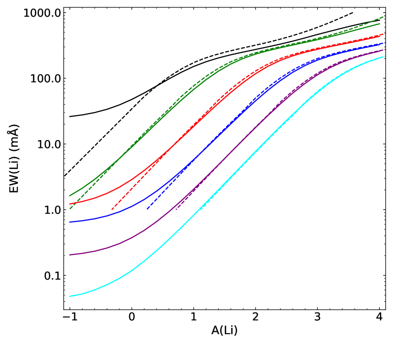
Figure 3: Comparison of the COGs from Soderblom et al. (1993, dashed lines) with our FGK COGs (solid lines) for the corresponding parameters ($\log g=4.5$ and solar metallicity). COGs are plotted for $T_{\mathrm{eff}}=4000$, 4500, 5000, 5500, 6000, and 6500 K (from top to bottom).

In Fig. 3 we compare the COGs for solar metallicity and $\log g=4.5$ with those of Soderblom et al. (1993), for different values of $T_{\mathrm{eff}}$ between 4000 and 6500 K. There is an excellent agreement between the two sets, except at low abundances or for $T_{\mathrm{eff}}=4000$ K, likely due to the differences in the way the COGs were measured. The discrepancies at 4000 K are also due to the difficulty of deblending the individual Li and Fe lines from the other line and molecular blends at solar metallicity.

3.2 M-type stars

According to the Milky Way and cluster target selection function (see Stonkutė et al., 2016; Bragaglia et al., 2022), M-type stars in GES are generally observed only with Giraffe HR15N and not with UVES (except for a handful of objects), and they are mainly young objects that may have large rotation rates. Therefore COGs in this regime are required for Giraffe HR15N only, and rotation must also be taken into account.

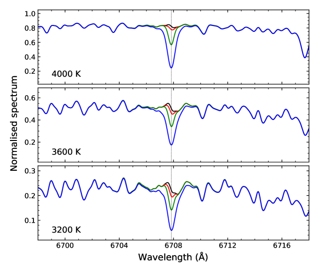
Figure 4: Synthetic spectra of M-type dwarf stars with $T_{\mathrm{eff}}=4000$, 3600 and 3200 K (from top to bottom), $\log g=4.5$ and solar metallicity, at the Giraffe resolution. Spectra are plotted for $A\mathrm{(Li)}=-1.0$ (black line), 0.0 (red line), $+1.0$ (green line), and $+3.0$ (blue line). The vertical dotted line shows the mean position of the lithium doublet.

To measure the COGs, we degraded the spectral grid for $T_{\mathrm{eff}}\leq 4500$ K at the Giraffe resolution. In Fig. 4 we show an example of the synthetic spectra for three temperatures and different lithium abundances. The figure clearly shows the increasing depression of the pseudo-continuum level going towards lower temperatures, and the strong blending with other components that dominate the absorption when the lithium line is weak or not present. A local pseudo-continuum was defined as the envelope of the molecular bands, approximated by a straight line passing through the maxima of the spectra on both sides of the lithium line. Analysis of the synthetic spectra shows that these maxima are generally located in the wavelength intervals [6703.0, 6705.0] Å and [6710.0, 6712.0] Å for slow rotators. To account for the different rotation rates of the target stars, COGs were measured for nine different rotational velocities from 0 to 150 km s^-1. However, the full set of rotational velocities could only be measured for $A(\mathrm{Li})>2.0$. At lower abundances the maximum $v\sin i$ was set to lower values, as indicated in Table 1. We also limited $v\sin i$ to 50 km s^-1 for giants with $\log g<3.5$, since higher rotational velocities are generally not found in these stars.

Table 1: Maximum allowed $v\sin i$ in M-type COGs

Max. $v\sin i$	Range
(km s-1)
150	$A(\mathrm{Li})>2.0$
100	$1.0<A(\mathrm{Li})<2.0$
50	$0.0<A(\mathrm{Li})<1.0$
30	$A(\mathrm{Li})<0.0$
50	$\log g<3.5$

The pEW was then derived by direct integration within a specified wavelength interval, which was defined as a symmetric interval of width $\pm d$ around $\lambda_{\mathrm{Li}}=6707.84$ Å. The value of $d$ was derived by measuring the full width of the lithium line in the synthetic spectra, and was also verified using observed spectra. For slow-rotators we found $d=0.8$ Å: this width is appropriate up to a projected rotational velocity $v\sin i=20$ km s^-1. Above this threshold, the line broadens according to the following relation:

$$d=0.8+0.02\,(v\sin i-20)\;\text{\AA}.$$ (1)

We checked that this interval is also consistent with the typical width of the lithium line in Giraffe spectra of FGK stars, hence no major inconsistencies are expected between the two regimes. The derived COGs are given in Table 8.

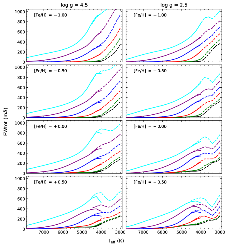
Figure 5: Comparison of the measured total EW (Li+Fe) vs $T_{\mathrm{eff}}$ for FGK (solid lines) and M-type stars with $v\sin i=0$ (dashed lines), for $\log g=4.5$ (left panels) and 2.5 (right panels), and different metallicities. The COGs are plotted for $A(\mathrm{Li})=-1.0$ (black), 0.0 (green), $+$1.0 (red), $+$2.0 (blue), $+$3.0 (purple), and $+$4.0 (cyan).

Figure 5 compares the two sets of COGs for dwarfs ($\log g=4.5$) and giants ($\log g=2.5$) at different metallicities. For the FGK regime, the total Li+blends EW is plotted. The plots show that the two sets connect smoothly, implying that homogeneity is ensured. As mentioned before, the discrepancies seen at 4000-4250 K are due to the difficulty of measuring the individual Li and Fe EWs at these temperatures, especially at higher metallicities where molecular blends are already important. This problem appears to be stronger for dwarfs than for giants, because of the stronger molecular lines present in dwarf stars. For this reason, in this temperature interval it is advisable to adopt the integration method and the M-type COGs, if possible. The dip seen at $\sim$ 3500 K was already noted by Palla et al. (2007), and is likely due to changes in the relative contribution of TiO bands and lithium. We also note that, because of the presence of the additional line components blended with lithium that are included in the integration interval (see Fig. 4), the pEW can never be equal to zero, even when no lithium line is present. For a non-rotating dwarf star at solar metallicity the pEW for $A(\mathrm{Li})=-1.0$ ranges from $\sim$ 50 mÅ at 4000 K to $\sim$ 300 mÅ at 3000 K.

4 Lithium measurements

Lithium measurements on GES spectra were performed as consistently as possible with the way the COGs were derived. The EWs and pEWs were generally measured only for stars with signal-to-noise ratio S/N$\,>10$ (or 20 in some cases), except for young stars with strong lithium absorption, where we lowered the limit to S/N$\,>5$ whenever possible. In addition, measures were generally limited to $v\sin i\la 100$ km s^-1 in Giraffe and 50 km s^-1 in UVES, unless the line was sufficiently strong to be also measurable at higher rotation rates. The lower threshold adopted for UVES is due to the fact that the bulk of the stars observed with the U580 setup have $v\sin i<20$ km s^-1, and the number of objects above the threshold with a measurable Li line is small. We also excluded spectra with clear evidence of double (or multiple) lines, indicative of SB2 binaries, or SB1 binaries with large velocity variations, for which the derived parameters are likely not accurate. Before performing the measurements, spectra were shifted to a rest frame based on their radial velocities.

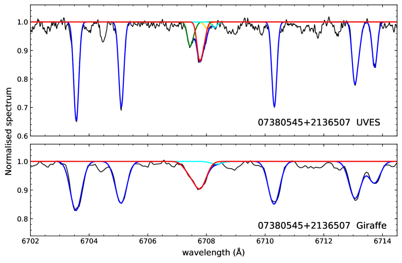
Figure 6: Best-fit results for the UVES (upper panel, S/N = 119) and Giraffe (lower panel, S/N = 223) spectra of the giant star 07380545+2136507 shown in Fig. 1 ($T_{\mathrm{eff}}=4899\pm 34$ K, $\log g=2.80\pm 0.05$, $\mathrm{[Fe/H]}=-0.17\pm 0.05$). In the upper panel, the red and green lines show the best-fit lithium and Fe blend components, respectively, while in the lower panel only the combined Li+Fe component is shown in red. The gold and cyan lines are the best-fit components at $\sim$ 6708.0 and 6708.3 Å. The total fit including the additional lines (see text) is marked in blue. The measured EWs are EW(Li)$\,=40.0\pm 0.8$ mÅ, EW(Fe)$\,=22.8\pm 0.8$ mÅ for UVES, and EW(Li+Fe)$\,=64.6\pm 1.1$ mÅ for Giraffe. The resulting lithium abundances are $A(\mathrm{Li})=1.25\pm 0.04$ for UVES and $1.30\pm 0.05$ for Giraffe.

4.1 Continuum level

As mentioned in Sects. 3.1 and 3.2, the local continuum or pseudo-continuum was approximated as a straight line, passing through the maxima of the spectrum at the two sides of the lithium line. These maxima were searched in the intervals [6701.0, 6705.5] Å and [6709.5, 6715.0] Å for FGK stars, and in the intervals defined in Sect. 3.2 for M-type stars. The larger intervals used for FGK stars account for the blending of lines in Giraffe spectra, which can slightly depress the continuum around lithium in high-metallicity or giant stars. To identify the position of the maxima, we performed a non-parametric fit of the spectra within the two intervals, using a median filter with a variable smoothing window depending on the S/N, and calibrated separately for UVES and Giraffe (to account for the different resolution), and for M-type stars (to account for the differences in the spectra). In some cases, in particular for young stars in regions affected by nebular emission, or when residual spurious features were present, the automatic identification of the continuum failed: in such cases, we searched the maximum in a small interval of $\pm 0.5$ Å around a manually fixed wavelength position at one or both sides of the lithium line. We caution that the positioning of the continuum at low S/N ($<20$) may not be accurate because of the strong noise, and the corresponding EWs may be overestimated or underestimated by up to 20-30 mÅ. These cases are not specifically flagged in the final catalogue, but they can be identified using the S/N values provided in the SNR column.

Table 2: Components used in the spectral fit for FGK stars

Component	Element	$\lambda$ (Å)	UVES	Giraffe
Li line	Li i	6707.761	✓	✓
	Li i	6707.912	✓	✓
Fe blend	Fe i	6707.431	✓	✓
	V i	6707.518	✓	✓
	Cr i	6707.596	✓	✓
Comp. 1	Si i	6708.023	✓
	V i	6708.094	✓
Comp. 2	Fe i	6708.282	✓	✓
	Fe i	6708.347	✓	✓

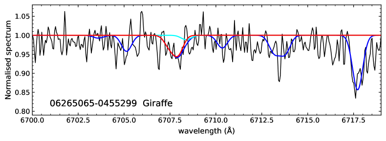
Figure 7: Best-fit result for the spectrum of the metal-poor star 06265065-0455299 observed with Giraffe (S/N = 33). This star has $T_{\mathrm{eff}}=5565\pm 95$ K, $\log g=3.79\pm 0.39$, $\mathrm{[Fe/H]}=-0.74\pm 0.14$, EW(Li+Fe)$\,=52.4\pm 8.7$ mÅ, and $A(\mathrm{Li})=2.10\pm 0.13$. Line colours are the same as the bottom panel of Fig. 6.

4.2 EW measures

In the case of FGK stars, EWs were measured by fitting the spectra, normalised by the local continuum and shifted to the rest wavelength, with a combination of Gaussian components. We adopted the same code for UVES and Giraffe, with only some slight differences due to the different spectral resolution of the two instruments. The fit was performed using the lmfit python package (Newville et al., 2014), which provides a simple framework to perform a non-linear least-squares fit of complex models with several components, allowing users to easily change, fix or tie the different model parameters. This method was applied for $T_{\mathrm{eff}}\geq 4000$ K to all UVES spectra and to Giraffe spectra with $\mathrm{[Fe/H]}<-1.5$, for which M-type COGs were not computed and only FGK COGs are available. For the remaining Giraffe spectra, we used this method for stars with $T_{\mathrm{eff}}>4250$ K, that is, we set the threshold between the FGK and M regimes in the middle of the overlapping region of the two COGs. This choice allowed us to ensure better continuity between the measures in the two regimes, and to derive the abundances and their uncertainties using the same COG.

The components used for the fit around the lithium position are consistent with the linelist of Guiglion et al. (2016), which was used to generate the synthetic spectral grid, and are indicated in Table 2. For lithium, we fitted the two components of the doublet separately. The Fe blend includes two additional lines besides the Fe i line, which are generally weak but contribute to the global line shape. In addition, we also included two other components at $\sim$ 6708.0 and $\sim$ 6708.3 Å. These components amount generally to a few mÅ, but can become significant as temperature decreases at solar and super-solar metallicities and/or for enhanced abundances with respect to solar of the corresponding species, and they are required to fit correctly the lithium line at low abundances. The component at $\sim$ 6708.0 Å was only used for UVES, since at the Giraffe resolution it is completely blended with lithium and cannot be constrained. In the fit, the widths of all lines were tied together, and we fixed their relative position with respect to the first line of the lithium doublet, allowing the latter to vary slightly in wavelength to allow for possible uncertainties in the radial velocity correction. In addition to the lines listed in Table 2, a set of relatively strong Fe lines between 6703.6 and 6713.7 Å, and, for Giraffe only, the Ca i line at 6717.69 Å, were also included in the fit to better constrain the Gaussian widths. An example of the fit for UVES and Giraffe is shown in Fig. 6, where we plot the best-fit results for the spectra of Fig. 1. In Fig. 7 we show a more problematic case, for a metal-poor star observed with Giraffe at S/N$\sim$30, where the fit is constrained by the Ca i line.

The EWs of each component were derived from the amplitudes of the best-fit Gaussians. In the case of UVES, the Li-only EW was simply obtained by summing the two lithium components. In a few cases, where the lithium line was very strong, the fit failed, artificially enhancing the 6708.0 Å line and reducing the Li contribution: when this happened, the EW of the 6708.0 Å line was combined with the Li EW to produce the final measure. In the case of Giraffe, or for UVES spectra with high rotation, the blended Li+Fe EW was obtained by combining the EWs of the Li and Fe components; for UVES, we also added the 6708.0 Å component, which is generally zero but sometimes, when the line is strong, is enhanced by the fit compensating the lithium line, as mentioned above. Uncertainties on the measured EWs were computed by means of the Cayrel (1988) formula, which however assumes no uncertainty in the continuum placement, using the FWHM derived from the best-fit. For a few stars with large rotation rates observed with Giraffe, the Gaussian fit was not acceptable: in these cases, a direct integration was used, adopting the same interval defined for M-type stars, and uncertainties were computed using the error propagation formula on the EW.

In M-type stars, the pEW were measured by direct integration over the interval defined in Sect. 3.2. As mentioned above, this method was used for Giraffe spectra with $T_{\mathrm{eff}}\leq 4250$ K and $\mathrm{[Fe/H]}\geq-1.5$. We checked that above this temperature threshold the integrated pEW is consistent, within a few mÅ, with the EW obtained using the Gaussian fit for spectra with S/N$\,>30$ and low rotation rates. At lower S/N, noise starts to affect the integrated values, while at high rotation rates the widening of the integration interval starts to include additional components that may not be fully taken into account in FGK stars. Direct integration was also used for stars with no derived $T_{\mathrm{eff}}$ that showed a clear M-type spectrum. Uncertainties were derived using the error propagation formula on the EW.

Figure 8 shows the distribution of the derived uncertainties on EW or pEW and their dependence on S/N for Giraffe and UVES separately. In the case of UVES, uncertainties are generally lower than 5 mÅ (except for S/N $<20$, where they can reach $\sim$ 10 mÅ), with the bulk of them concentrated between 1 and 2 mÅ. Uncertainties on Giraffe EWs are larger, with a median of $\sim$ 6 mÅ and a long tail reaching some tens of mÅ for low S/N spectra.

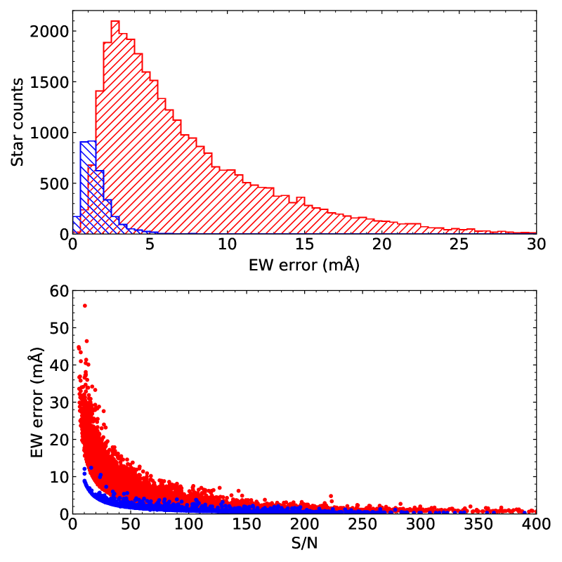
Figure 8: Uncertainties on EW or pEW. In the top panel, we show the distribution of the uncertainties for Giraffe (red hatched histogram) and UVES (blue hatched histogram). In the bottom panel, we plot the uncertainties on EW or pEW as a function of the S/N. Colours are the same as the top panel, and the plot was limited to S/N$\,<400$ for better clarity. Uncertainties are higher for stars with higher rotational velocity.

4.3 Upper limits

Upper limits were automatically assigned whenever the measured EW or pEW was lower than the corresponding uncertainty. In these cases, the uncertainty value was taken as upper limit. We further visually inspected all cases with S/N$\,<30$ or EW$\,\la 50$ mÅ, and assigned upper limits equal to the measured EW when the line was not or barely visible.

Since the visual identification of upper limits may be subjective and prone to errors, especially in noisy spectra, in the case of UVES we devised a procedure that allowed us to identify secure upper limits and detections in a semi-automatic way. To this aim, we computed the difference between the medians of the residuals of the fit obtained with and without the Li component in the interval [6707.7, 6707.95] Å, and we divided it by the standard deviation of the residuals of the fit with lithium. We assumed this standard deviation to represent a reasonable estimate of the noise level, instead of considering a continuum region free of lines, because of the difficulty to find a suitable region valid for the large variety of GES spectra. This procedure was tested on a sub-sample of spectra, and we found that when the derived ratio is $>2$ the lithium line is generally present, while when the ratio is $<1.7$ for giants and $<1.4$ for dwarfs the line is generally undetectable. Between these two thresholds most cases are upper limits, but detections can also be found, and visual inspection was still required. Applying the above criteria to the whole sample of UVES spectra allowed us to identify additional upper limits that were previously considered as dubious detections. This procedure is not entirely free from errors, and we cannot exclude that some misclassifications might still be present, however we estimate that less than 1% of the sample might be affected.

The extension of the method described above to Giraffe spectra is not straightforward, because the blend can be detected when the Fe line is visible even if lithium is not, and it was not possible to find a reasonable criterion to identify secure upper limits. Therefore, in the case of Giraffe, upper limits were only assigned by visual inspection, and in doubtful cases the measures were generally kept as detections. We caution that, because of this, it is possible that some of the detections with low EW at S/N$\,<30$ might have been misclassified and be upper limits instead.

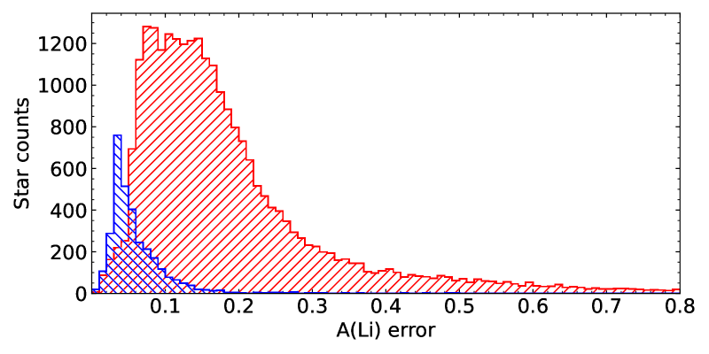
Figure 9: Distribution of the uncertainties on $A$(Li) for Giraffe (red hatched histogram) and UVES (blue hatched histogram).

4.4 Abundances

Lithium abundances were derived by interpolating the appropriate COGs at the temperature, gravity, and metallicity (and rotation for M-type stars) of each star, using the atmospheric parameters derived in the first pass of the spectral analysis (see Gilmore et al., 2022). The FGK COGs were used for all UVES spectra with $T_{\mathrm{eff}}\geq 4000$ K, for Giraffe spectra with $T_{\mathrm{eff}}\geq 4000$ K and $\mathrm{[Fe/H]}<-1.5$, and for Giraffe spectra with $\mathrm{[Fe/H]}\geq-1.5$ and $T_{\mathrm{eff}}\geq 4250$ K. For the remaining Giraffe spectra the M-type COGs were applied.

Abundances were only derived for stars for which atmospheric parameters falling inside the relevant COG grid are available. In particular, no abundances were computed if recommended values of $T_{\mathrm{eff}}$ or $\log g$ are not present. However, for stars observed with Giraffe HR15N, an indication of gravity is given by the $\gamma$ spectral index (Damiani et al., 2014): in the $\gamma$-$T_{\mathrm{eff}}$ diagram, giants occupy a well defined region clearly distinct from dwarfs. Therefore, for stars with no $\log g$ but with a measured $\gamma$ index, we assumed $\log g=2.5$ if $T_{\mathrm{eff}}<5400$ K and $\gamma>0.98$ (see e.g. Bravi et al., 2018), and $\log g=4.5$ otherwise. This is obviously an approximation, in particular for PMS stars that would have an intermediate $\log g$, and we caution that the derived abundances may not be accurate, especially if the true $\log g$ differs significantly from the assumed value. For some stars in young open clusters with $\log g>5.0$, we computed the abundance using $\log g=5.0$.

When a recommended value of [Fe/H] was not available, we assumed a solar metallicity. While this assumption is reasonable for many of the open clusters in our sample, it is clearly incorrect for metal-rich or metal-poor stars, and in particular for stars in globular clusters. This assumption should not significantly affect results from UVES spectra, since blends are believed to weakly contribute to the EW measurement, but it could lead to an overestimate or underestimate of the Fe-blend correction in Giraffe spectra, and therefore to an underestimated or overestimated abundance.

In the case of FGK stars, when the deblended lithium line could be directly measured, abundances were derived by simply interpolating the FGK COGs. If only the Li+Fe blend could be measured, we first applied the blend correction to derive the Li-only EW before computing the abundance; for these stars, both EW(Li+Fe) and EW(Li) are provided. The correction was not applied to upper limits: in this case we set an upper limit to EW(Li) equal to the total Li+Fe upper limit. The same upper limit to EW(Li) was also set when the corrected EW was lower than the uncertainty, and the derived abundance was considered an upper limit too. For M-type stars, COGs were applied directly to the measured pEW. In all cases, whenever the EW or pEW was lower than the minimum allowed value in the interpolated COG, we set an upper limit $A(\mathrm{Li})<-1.0$. However, the lithium abundance was extrapolated above $A(\mathrm{Li})=4.0$ if necessary.

The spectra of young stars with significant accretion are affected by veiling: accretion produces an excess continuum which results in a lower measured EW. For these stars, the measure of the ratio $r$ between the excess and photospheric continuum is provided by the OACT node in WG12 for Giraffe spectra (see Lanzafame et al., 2015). For stars for which $r$ is significant (i.e. $r$ greater than its uncertainty) we corrected the measured Giraffe EW or pEW using the formula EW${}_{\mathrm{true}}=(1+r)\,$EW_measured; the abundance was then computed from the corrected EW. In these cases, the uncertainty on the corrected EW was derived by combining the original EW error and the error on $r$ in quadrature. However, we did not compute any abundance if $r>1$, since these high values of $r$ might be inaccurate.

Random uncertainties on the abundances (for detections only) were derived taking into account the uncertainties on EW or pEW and on the stellar parameters ($T_{\mathrm{eff}}$, $\log g$ and [Fe/H]). To this aim, we varied one parameter at a time by its error and derived the corresponding uncertainty in the abundance. The individual uncertainties were then combined in quadrature to derive the final uncertainty. The dominant contribution to the abundance uncertainties is due to the uncertainties in EW and $T_{\mathrm{eff}}$, while the effect of the other parameters is generally small. In Fig. 9 we show the distribution of abundance uncertainties for UVES and Giraffe separately. As expected, UVES abundances are more precise, with a median uncertainty of $\sim$ 0.05 dex. The Giraffe distribution is wider, with a median of $\sim$ 0.15 dex, and an extended tail with a few errors $>1$ dex, although the bulk of measures have uncertainties lower than 0.3 dex.

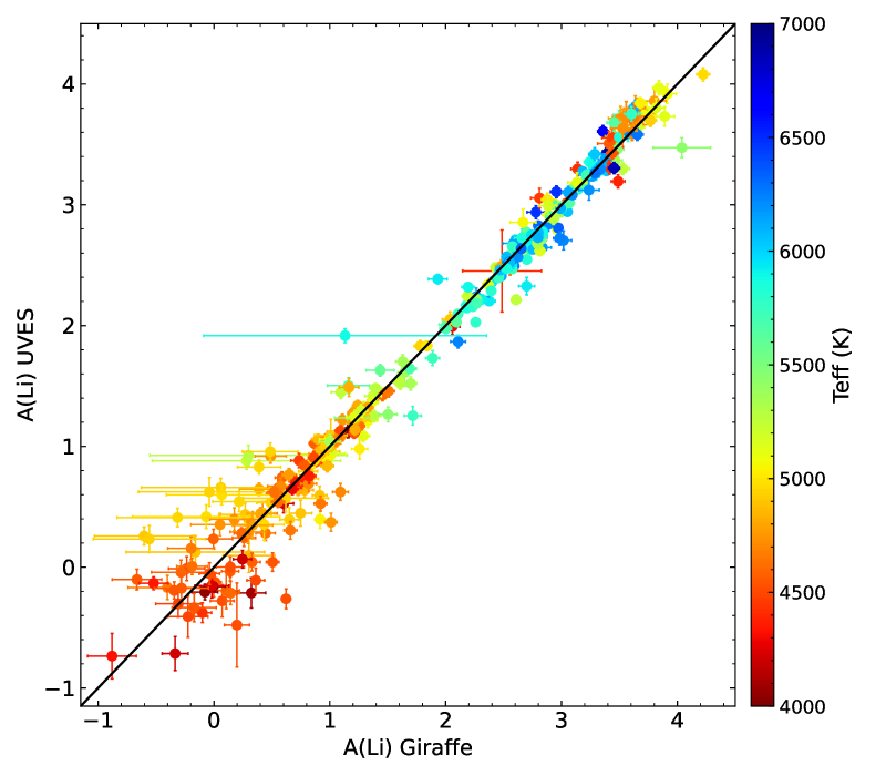
Figure 10: Comparison of the lithium abundances derived for stars observed with both UVES and Giraffe. Points are colour-coded by $T_{\mathrm{eff}}$. Only stars with detections in both instruments are plotted.

In Fig. 10 we compare the abundances derived for stars observed with both UVES and Giraffe, for which lithium was detected in both instruments. There is in general a very good agreement between the results, at least for $A(\mathrm{Li})>1.0$, with a larger scatter at lower abundances. A 3-$\sigma$ clipped average of the differences between UVES and Giraffe over the entire range gives a mean of $+0.01$ dex with a standard deviation of 0.13 dex. The standard deviation reduces to 0.10 dex for $A(\mathrm{Li})>1.0$ and increases to 0.29 dex at lower abundances, with no significant change in the means ($+0.00$ and $-0.01$ dex, respectively). The outliers with a large error in Giraffe are mostly giant stars where the lithium line is very weak and the detection in Giraffe is dominated by the iron line: in these cases, the measure is likely not accurate, and the blend-corrected EW is very close to the uncertainty, resulting in large errors on the derived abundances.

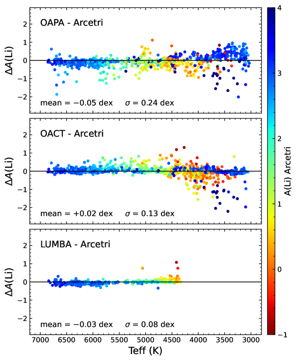
Figure 11: Comparison between the abundances derived by Arcetri with those derived by other nodes as a function of $T_{\mathrm{eff}}$, for stars observed with Giraffe. The plotted differences $\Delta\,A(\mathrm{Li})$ are computed as the other node minus Arcetri, and are colour-coded by the Arcetri abundance. Only stars with detections in both nodes are plotted. The 3-$\sigma$ clipped average and standard deviation of the abundance differences are indicated in the respective panels.

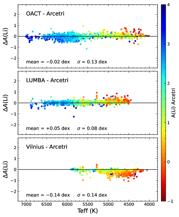
Figure 12: Same as Fig. 11 but for stars observed with UVES.

5 Validation

5.1 Internal validation

To validate our results, we compared them with the abundances provided by other GES analysis nodes in their respective working groups, namely OAPA (WG12), OACT (WG10, WG11, and WG12), LUMBA (WG10 and WG11), and Vilnius (WG11). In the case of UVES, the full dataset was analysed by all contributing nodes. For Giraffe, the other nodes were asked to provide measures only for the two open clusters NGC 2420 and NGC 2516 and the PMS $\lambda$ Ori cluster. The OAPA and OACT nodes measured lithium using the EW method, with their own codes but following the rules described here and converting the EWs to abundances using the set of COGs provided in this paper. The LUMBA and Vilnius nodes used instead spectral synthesis to derive directly the lithium abundances.

Figure 11 shows the differences between the abundances derived by Arcetri and by the other nodes for Giraffe spectra. There is a general good agreement between the nodes, although with a larger spread for the nodes using the EW method. The strong outliers in the comparison with the OAPA and OACT nodes are generally due to stars with high rotation, low $T_{\mathrm{eff}}$, or low S/N, where the measure can be complicated and is strongly affected by the choice of the continuum, or, in a few cases, to stars with wrong radial velocity where the lithium line might have been misidentified. Some of the discrepant cases at $T_{\mathrm{eff}}<4000$ K are due to stars affected by veiling that were probably not corrected by the other nodes. There is a tendency for OAPA to overestimate the abundances of M-type stars with respect to Arcetri, and for OACT to underestimate them. However, the differences are relatively uniform at all temperatures and the average difference is very small in both cases: the 3-$\sigma$ clipped average is $-0.05$ dex for OAPA and $+0.02$ dex for OACT, with standard deviations of $\sim$ 0.1$-$0.2 dex. In the case of LUMBA we consider only FGK stars, since the method used by this node is not able to provide reliable results for M-type stars. The few outliers are giant stars with $\log g<3.1$, for which the LUMBA abundances appear to have been overestimated, probably because of an erroneous identification of the lithium detection when the close Fe blend is strong. Apart from these objects, there is a very good agreement between LUMBA and Arcetri: the average difference is $-0.03$ dex with a standard deviation of $0.08$ dex.

Figure 12 shows the same comparison for UVES spectra. Again, the agreement with OACT and LUMBA is very good, with average differences of $-0.02$ and $+0.05$ dex, respectively, and standard deviations of $\sim$ 0.1 dex. On the other hand, the Vilnius node tends to provide lower abundances for $T_{\mathrm{eff}}<5000$ K, which results in an average difference of $-0.14$ dex. These stars are mostly giants with very low lithium abundances, whose measure is strongly dependent on the choice of the continuum level. Considering only stars with $T_{\mathrm{eff}}>5000$ K, the mean difference reduces to $-0.07$ dex with a dispersion of 0.10 dex.

In summary, the agreement of our abundances with those derived from other nodes is very good for both instruments, with differences of at most $\pm 0.05$ dex, which are consistent or lower than the average abundance uncertainties. Such differences can be expected considering differences in the continuum placement and in the measurement method adopted by the different nodes.

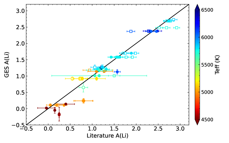
Figure 13: Comparison of the average GES abundances for benchmark stars with those from the AMBRE project (open squares, Guiglion et al., 2016) and from other literature studies (filled circles, see text). Only stars with detections in GES and in the literature studies are plotted. Data are colour-coded by the GES temperature. Points aligned on the same horizontal line refer to multiple measures of the same star.

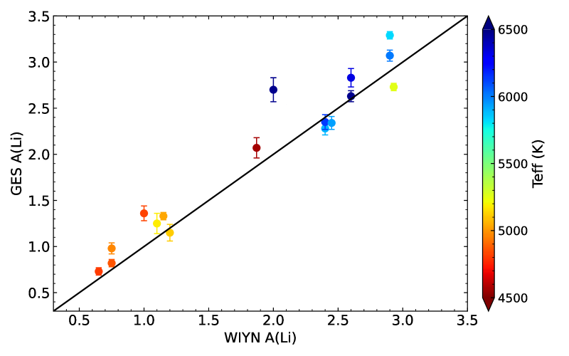
Figure 14: Comparison of the GES recommended abundances with those derived from the WIYN Open Cluster Study for stars in IC 2391 and NGC 2243 (Platais et al., 2007; Anthony-Twarog et al., 2021). Only stars with detections in both samples are shown. Data are colour-coded by the GES temperature. Uncertainties on the WIYN abundances are not available.

Table 3: Lithium-related columns in the final catalogue

Column name	Units	Description
LI1	dex	Neutral lithium abundance
LIM_LI1		Flag on LI1 measurement (0=detection, 1=upper limit)
E_LI1	dex	Error on LI1
EW_LI	Å	Total Li(6708Å) equivalent width or pseudo-equivalent width including blends
LIM_EW_LI		Flag on EW_LI (0=detection, 1=upper limit)
E_EW_LI	Å	Error on EW_LI
EWC_LI	Å	Blends-corrected Li(6708Å) equivalent width
LIM_EWC_LI		Flag on EWC_LI (0=detection, 1=upper limit)
E_EWC_LI	Å	Error on EWC_LI

Table 4: Lithium-specific TECH flags in the final catalogue

Flag	Description
10110-wg-01-01	Over- or under-subtracted sky features at the position of the Li line
12003-wg-01-01	Li abundances are not provided because $\log g$ is not available
12004-wg-01-00—17103-wg-01-01	Metallicity is not provided and the solar value is used
12005-wg-01-01	Li not measured because $v\sin i>50$ km s-1
12005-wg-01-02	Li not measured because $v\sin i>100$ km s-1
12009-wg-01-01	Li line not measurable in stars with $T_{\mathrm{eff}}>8000$ K
12010-wg-01-01	Li abundance is not provided because some parameters are outside the COG grid
12012-wg-01-01—17103-wg-01-02	Gravity is not provided and it was estimated using the $\gamma$ index (see text)

5.2 External validation

In addition to the above analysis, we also compared our results for benchmark stars with the abundances available in the literature. The GES sample contains a set of UVES and Giraffe spectra of the Sun. We derived an average lithium abundance of $1.07\pm 0.02$ dex for UVES and $1.06\pm 0.10$ dex for Giraffe. Both values are in very good agreement with the solar abundance of $1.05\pm 0.10$ dex derived by Grevesse et al. (2007). In Fig. 13 we compare the GES recommended abundances (see Sect. 6) of other benchmark stars with those obtained by the AMBRE project (Guiglion et al., 2016) and by other studies available in the literature (Lèbre et al., 1999; Mallik, 1999; Takeda et al., 2007; Mentuch et al., 2008; Baumann et al., 2010; Gonzalez et al., 2010; Ramírez et al., 2012; Delgado Mena et al., 2014, 2015; Bensby & Lind, 2018; Chavero et al., 2019; Charbonnel et al., 2020). For most stars, multiple measures are available in the literature, with a significant spread. However, on average there is an excellent agreement between our abundances and the literature ones; a 3$\sigma$-clipped average of the differences between GES and literature values gives a mean of $-0.07$ dex with a standard deviation of 0.20 dex.

Our sample contains 213 stars with detected lithium abundance that are in common with the GALAH (GALactic Archaeology with HERMES) DR3 catalogue (Buder et al., 2021), considering only GALAH objects with flag_sp=0 and flag_li_fe=0. However, a direct comparison between the two datasets is not straightforward, because the abundances provided by GALAH were derived in non-LTE: to do so, we would have to convert our abundances using non-LTE corrections, which are model-dependent and could introduce a bias. Therefore, we decided not to perform the comparison here.

Finally, in Fig. 14 we compare the GES recommended abundances of stars in the open clusters IC 2391 and NGC 2243 with those derived in the context of the WIYN Open Cluster Study (Platais et al., 2007; Anthony-Twarog et al., 2021), for the 17 stars in common with detections in both samples. Also in this case the agreement is good, although the GES abundances tend to be slightly higher on average, with a mean difference of 0.13 dex and a dispersion of 0.22 dex.

Table 5: Number of lithium detections (det.) and upper limits (u.l.), for the full sample and divided by target types.

	GES_TYPE	$N_{\mathrm{abund}}$	$N_{\mathrm{EW}}$	LI1		EW_LI		EWC_LI
				det.	u.l.	det.	u.l.	det.	u.l.
Total	All	38081	40079	27250	10831	30445	4002	23894	9742
Open clusters	*_CL/*_SD_OC	30230	32149	22639	7591	26781	3873	19479	6662
Globular clusters	*_SD_GC	1240	1262	869	371	892	19	879	346
Milky Way fields	GE_MW/GE_MW_BL	3345	3393	1521	1824	7	0	1555	3087
Corot & Kepler2 fields	GE_SD_CR/GE_SD_K2	3206	3212	2169	1037	2751	110	1933	893
Benchmark stars	others	60	63	52	8	14	0	48	3

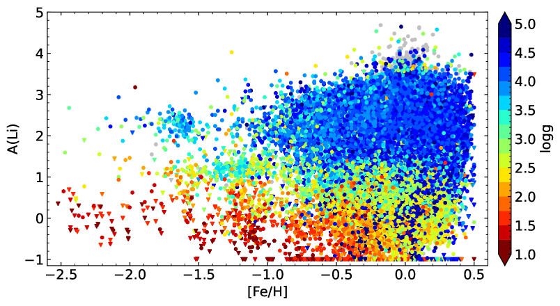
Figure 15: Full sample of lithium abundances as a function of metallicity. Values are colour-coded by $\log g$. Grey points mark young stars for which no $\log g$ is available. Downward triangles indicate upper limits.

6 The final catalogue

The results obtained in Sect. 4 were combined together to produce the final catalogue. As a first step, for each setup we first combined the measures obtained from multiple spectra of the same star, which were available for benchmark stars and for a few open cluster stars with archival observations in addition to the GES ones. For these cases, if one or more detections were available, we took as final value the average of the detections (for both EWs and abundances), and the average error as uncertainty. This procedure was also applied when a mix of detections and upper limits for the same star was present. If only upper limits were present, we took the highest upper limit as final value, to be conservative. We then merged the results obtained from UVES and Giraffe. UVES measures were retained only for $T_{\mathrm{eff}}\geq 4000$ K, since EWs measured at lower temperatures are not reliable and abundances were not derived. When results from both instruments were available, we took preferentially the UVES measures as recommended values, since they are more precise. Otherwise, the only available UVES or Giraffe measures were taken as recommended values.

Table 3 lists the lithium-related columns available in the catalogue. Lithium abundances are given in the LI1 column, with associated columns for the errors and flags. In addition, we also provide the measured EWs. EW_LI contains the measured total EW (including blends) for FGK stars, or the measured pEW for M-type stars with $T_{\mathrm{eff}}\leq 4250$ K and [Fe/H] $\geq-1.5$. EWC_LI contains the Li-only EW, either directly measured in UVES (in this case EW_LI is empty), or derived from EW_LI using the blend corrections after the eventual correction for veiling. EWC_LI is empty for M-type stars for which the pEW is given in EW_LI, or when the abundance could not be derived. In addition to these columns, veiling measures are also available in the columns VEIL and E_VEIL. The catalogue also contains a set of technical flags in the TECH column, and peculiarity flags (e.g. for binaries) in the PECULI column. In Table 4 we only list the TECH flags specific to the lithium measurements, but other generic flags on S/N or problems in the spectra may also be present.

The final catalogue at ESO contains lithium EW measures or upper limits for a total of 40 079 stars, and lithium abundances for 38 081 stars. The number of available measures for the different sub-sample types is given in Table 5, and the distribution of lithium abundances as a function of metallicity and gravity is shown in Fig. 15. The vast majority of the sample ($\sim\,$80%) consists of stars observed in the fields of open clusters spanning a large age range, from a few Myr up to $\sim\,$9 Gyr, and covering a wide range of Galactocentric distances (see Randich et al., 2022); in addition, about 3% of the lithium measures were obtained for stars in globular clusters. The remaining 17% are field stars, including stars in the Bulge and in Corot and Kepler2 fields. The sample covers well all evolutionary phases in the HR diagram, from PMS stars to giants, and also includes metal-poor stars on the Spite plateau. Therefore, this catalogue constitutes an invaluable dataset for the investigation of various topics, including membership of young clusters, determination of stellar ages, constraints on models of stellar structure and evolution, and Galactic evolution.

7 Caveats

As already mentioned in the previous sections, there are a few caveats that users of the catalogue should keep in mind when using the GES lithium dataset. We summarise them below.

The reported EWs for stars observed with Giraffe with $T_{\mathrm{eff}}\leq 4250$ K and [Fe/H] $\geq-1.5$ are pEWs that include molecular and other line blends. For this reason, pEWs do not go down to zero and may be significant even when no lithium is present (see Sect. 3.2). In addition to that, lithium-only EWs measured in UVES for $T_{\mathrm{eff}}\la 4250$ K and $\mathrm{[Fe/H]}\ga 0$ are strongly affected by blends and may not be accurate.

As noted in Sect. 4.3, EW upper limits for Giraffe and part of those for UVES were assigned after visual inspection of the fitted spectra. Because of this, some of the measures reported as detection for spectra with low S/N ($<30$) and weak lithium line (EW$\,\la 50$ mÅ) might have been misclassified and be upper limits instead.

The cut in $v\sin i$ described in Sect. 4 was applied using the values derived from the data reduction pipeline. Since some rotational velocities were revised after the spectral analysis, especially for the hotter stars, the final catalogue contains a few lithium measures with low EW at $v\sin i>150$ km s^-1. For part of them, the original rotational velocity was significantly underestimated, and the corresponding lithium measures might be inaccurate.

As discussed in Sect. 4.4, if a recommended metallicity was not available, the solar metallicity was used when computing lithium abundances. If the true metallicity is significantly different, the use of the solar value results in wrong abundances. This is especially true in the case of Giraffe, where the blend correction can be severely over- or underestimated. A similar problem holds for stars with no recommended $\log g$ value, where an approximated gravity was assumed based on the $\gamma$ index, if available: as above, if the true gravity is significantly different from the assumed one, the corresponding abundance is likely wrong. These cases are appropriately flagged in the final catalogue (see Table 4), and abundances for these stars should be taken with caution.

The measured Giraffe EWs for young stars affected by accretion were corrected for veiling before computing the abundances. However, estimating the veiling is not simple, and some of the reported values may be inaccurate: in this case, the derived lithium abundance may also be inaccurate. In particular, if the reported veiling is overestimated, the abundance will be overestimated as well. For this reason, we did not compute abundances if the veiling value was $>1$, and abundances for stars with veiling should be treated with caution.

A few cool stars in young clusters may have an underestimated value of $\log g$, indicative of giants, in contrast with the derived $\gamma$ index which is characteristic of dwarfs. Since abundances were derived using the $\log g$ value, the corresponding abundances for these stars might not be accurate. An example of this issue are the two members of the 25 Ori cluster mentioned in Sect. 3.5 of Franciosini et al. (2022), whose abundances might have been overestimated by $\sim 0.4-0.6$ dex.

Although clear SB2s were discarded from the sample before performing the measurements (see Sect. 4), some SB2s can only be detected by a careful exam of the cross-correlation function (Merle et al., 2017). In addition, a few SB2s were flagged by other nodes, or might have been identified in UVES but not in Giraffe for stars observed with both instruments. For such stars, the PECULI binarity flag 20020 is raised, and the corresponding lithium measurements, if present, are likely inaccurate.

We finally caution that, if the comparison with evolutionary models is made using EWs rather than abundances, the COGs provided here should be used to convert the model abundances into EWs. This is particularly true in the M dwarf regime; using a different set of COGs would result in inconsistencies between the measures and the models, leading to possibly inaccurate conclusions.

8 Summary

This paper describes the derivation of lithium abundances for the final data release of the GES. Lithium was measured on spectra obtained with both the Giraffe and UVES instruments, and covering a wide range of temperatures, gravity, and metallicity. We used an EW-based method, that is, we first measured the EW of the lithium line, and then we converted it to an abundance using a set of COGs that were specifically derived for GES. The COGs were measured on a grid of synthetic spectra covering the full range of parameters of GES observations, using a method consistent with that adopted to measure the EWs. The derived abundances are one-dimensional LTE abundances. We stress that our COGs represent the first set of homogeneously derived COGs over a wide range of temperatures (3000$-$8000 K), gravities ($\log g=$ 0.5$-$3.5), and metallicities ($-2.50\leq\mathrm{[Fe/H]}\leq+0.50$).

The presence of molecular blends in M-type stars, which increasingly affect the measure of lithium as temperature decreases, forced us to adopt two different methods for FGK and M-type stars. For FGK stars the lithium EW could be measured by fitting the line with Gaussian components, while for M-type stars a pEW was obtained by integrating the spectrum on a predefined interval. Care was taken to ensure that no significant discontinuity arises between the two temperature regimes. The derived abundances were validated using measures provided by other GES analysis nodes or available from the literature.

The final catalogue includes homogeneous lithium abundances and/or EWs for $\sim$ 40 000 stars distributed in all Milky Way components (open and globular clusters, disc, bulge and halo) and covering all evolutionary phases, from PMS stars to giants. This dataset will be very valuable for our understanding of several open issues, from stellar evolution and internal mixing in stars at different evolutionary stages, to the derivation of stellar ages, and to Galactic evolution. We finally note that the detailed work presented here will also be very useful for future large scale spectroscopic surveys, such as WEAVE and the 4MOST high-resolution stellar surveys, which will be characterised by a similar resolution as HR15N.

Appendix A Derived curves of growth

In Tables 6-8 (available in full at the CDS) we provide the derived COGs and blend corrections for FGK stars, and the COGs for M-type stars. The first ten lines of each table are shown here for reference.

Table 6: COGs for FGK stars

$T_{\mathrm{eff}}$	$\log g$	[Fe/H]	$A(\mathrm{Li})$	EW(Li)
(K)				(mÅ)
4000	0.5	$-$2.50	$-$1.0	5.38
4000	0.5	$-$2.50	$-$0.8	8.47
4000	0.5	$-$2.50	$-$0.6	13.28
4000	0.5	$-$2.50	$-$0.4	20.66
4000	0.5	$-$2.50	$-$0.2	31.78
4000	0.5	$-$2.50	0.0	48.06
4000	0.5	$-$2.50	0.2	70.95
4000	0.5	$-$2.50	0.4	101.78
4000	0.5	$-$2.50	0.6	139.13
4000	0.5	$-$2.50	0.8	181.39
…	…	…	…	…

Table 7: Blend corrections for FGK stars

$T_{\mathrm{eff}}$	$\log g$	[Fe/H]	EW(Fe)
(K)			(mÅ)
4000	0.5	$-$2.50	0.95
4000	0.5	$-$2.00	2.43
4000	0.5	$-$1.50	6.00
4000	0.5	$-$1.00	14.56
4000	0.5	$-$0.75	23.26
4000	0.5	$-$0.50	36.49
4000	0.5	$-$0.25	55.68
4000	0.5	$+$0.00	82.19
4000	0.5	$+$0.25	104.29
4000	0.5	$+$0.50	127.48
…	…	…	…

Table 8: COGs for M-type stars

$T_{\mathrm{eff}}$	$\log g$	[Fe/H]	$v\sin i$	$A(\mathrm{Li})$	pEW
(K)			(km s-1)		(mÅ)
3000	0.5	-1.50	0.0	$-$1.0	469.70
3000	0.5	-1.50	0.0	$-$0.8	482.25
3000	0.5	-1.50	0.0	$-$0.6	498.65
3000	0.5	-1.50	0.0	$-$0.4	518.97
3000	0.5	-1.50	0.0	0.0	568.76
3000	0.5	-1.50	0.0	0.2	595.87
3000	0.5	-1.50	0.0	0.4	622.93
3000	0.5	-1.50	0.0	0.6	649.38
3000	0.5	-1.50	0.0	0.8	675.05
3000	0.5	-1.50	0.0	1.0	700.05
…	…	…	…	…	…