Error analysis of a backward Euler positive preserving stabilized scheme for a Chemotaxis system

Abstract.

For a Keller-Segel model for chemotaxis in two spatial dimensions we consider positivity preserving fully discrete schemes which where introduced by Strehl et all. in [25]. We discretize space using piecewise linear finite elements and time by the backward Euler method. Under appropriate assumptions on the regularity of the exact solution, the spatial mesh and the time step parameter we show existence of the fully discrete solution and derive error bounds. We also present numerical experiments to illustrate the theoretical results.

1. Introduction

We shall consider a Keller-Segel system of equations of parabolic-parabolic type, where we seek $u=u(x,t)$ and $c=c(x,t)$ for $(x,t)\in{\Omega}\times[0,T],$ satisfying

(1.1) $$\begin{cases}u_{t}=\Delta u-\lambda\,div(u\nabla c),&\text{in }{{\Omega}}\times[0,T],\\ c_{t}=\Delta c-c+u,&\text{in }{{\Omega}}\times[0,T],\\ \frac{\partial u}{\partial\nu}=0,\;\;\;\frac{\partial c}{\partial\nu}=0,&\text{on }\partial{\Omega}\times[0,T],\\ u(\cdot,0)=u^{0},\quad c(\cdot,0)=c^{0},&\text{in }{{\Omega}},\end{cases}$$

where ${\Omega}\subset{\mathbb{R}}^{2}$ is a convex bounded domain with boundary $\partial\Omega$, $\nu$ is the outer unit normal vector to $\partial\Omega$, $\partial/\partial\nu$ denotes differentiation along $\nu$ on $\partial\Omega$, $\lambda$ is a positive constant and $u^{0},c^{0}\geq 0$, $u^{0},c^{0}\neq 0$.

The chemotaxis model (1.1) describes the aggregation of slime molds resulting from their chemotactic features, cf. e.g. [17]. The function $u$ is the cell density of cellular slime molds, $c$ is the concentration of the chemical substance secreted by molds themselves, $c-u$ is the ratio of generation or extinction, and $\lambda$ is a chemotactic sensitivity constant.

There exists an extensive mathematical study of chemotaxis models, cf. e.g., [22], [14], [15], [16], [26] and references therein. It is well-known that the solution of (1.1) may blow up in finite time. However, if $\|u_{0}\|_{L_{1}(\Omega)}\leq 4\pi\lambda^{-1}\pi,$ the solution of (1.1) exists for all time and is bounded in $L_{\infty}$, cg. e.g. [21].

A key feature of the system (1.1) is the conservation of the solution $u$ in $L_{1}$ norm,

(1.2) $$\|u(t)\|_{L_{1}}=\|u^{0}\|_{L_{1}},\quad 0\leq t\leq T,$$

which is an immediate result of the preservation of non-negativity of $u$,

(1.3) $$u^{0}\geq 0,\,\not\equiv 0\text{ in }\Omega\quad\Rightarrow\quad u>0\text{ in }\Omega\times(0,T],$$

and the conservation of total mass

(1.4) $$\int_{\Omega}\,u(x,t)\,dx=\int_{\Omega}\,u_{0}(x)\,dx,\;\;\;\;\;0\leq t\leq T.$$

Capturing blowing up solutions numerically is a challenging problem and many numerical methods have been proposed to address this. The main difficulty in constructing suitable numerical schemes is to preserve several essential properties of the Keller-Segel equations such as positivity, mass conservation, and energy dissipation.

Some numerical schemes were developed with positive-preserving conditions, cf. e.g. [13], [7], [6], which depend on a particular spatial discretization and impose CFL restrictions on the time step. Other approaches include, finite-volume based numerical methods, [7], [6], high-order discontinuous Galerkin methods, [11], [12],[19], a flux corrected finite element method, [25], and a novel numerical method based on symmetric reformulation of the chemotaxis system, [20]. For a more detailed review on recent developments of numerical methods for chemotaxis problems, we refer to [8] and [27].

In order to maintain the total mass and the non-negativity of the numerical approximations of the system (1.1), Saito in [23] proposed and analyzed a fully discrete method that uses an upwind finite element scheme in space and backward Euler method in time. His proposed finite element scheme made use of Baba and Tabata’s upwind approximation, see [1]. Strehl et al. in [25] proposed a slightly different approach. The stabilization was implemented at a pure algebraic level via algebraic flux correction, see [18]. This stabilization technique can be applied to high order finite element methods and maintain the mass conservation and the non-negativity of the solution.

In the variational form of (1.1), we seek $u(\cdot,t)\in H^{1}$ and $c(\cdot,t)\in H^{1},$ for $t\in[0,T]$, such that

(1.5) $$(u_{t},v)+(\nabla u-\lambda u\nabla c,\nabla v) =0,\quad\forall v\in H^{1},\quad\text{ with }u(0)=u^{0},$$

$$(c_{t},v)+(\nabla c,\nabla v)+(c-u,v) =0,\quad\forall\,v\in H^{1},\quad\text{ with }c(0)=c^{0},$$

where $(f,g)=\int_{\Omega}fg\,dx$.

In our analysis we consider regular triangulations $\mathcal{T}_{h}=\{K\}$ of $\overline{\Omega}$, with $h=\max_{K\in\mathcal{T}_{h}}h_{K}$, $h_{K}=\text{diam}(K)$, and the finite element spaces

(1.6) $$\mathcal{S}_{h}:=\left\{\chi\in\mathcal{C}:\chi|_{K}\in\mathbb{P}_{1},\forall K\in\mathcal{T}_{h}\right\},$$

where ${\mathcal{C}}={\mathcal{C}}(\overline{{\Omega}})$ denotes the continuous functions on $\overline{{\Omega}}$.

A semidiscrete approximation of the variational problem (1.5) is: Find $u_{h}(t)\in\mathcal{S}_{h}$ and $c_{h}(t)\in\mathcal{S}_{h}$, for $t\in[0,T]$, such that

(1.7) $$(u_{h,t},\chi)+(\nabla u_{h}-\lambda u_{h}\nabla c_{h},\nabla\chi) =0,\ \forall\chi\in\mathcal{S}_{h},\text{ with }u_{h}(0)=u_{h}^{0},$$

$$(c_{h,t},\chi)+(\nabla c_{h},\nabla\chi)+(c_{h}-u_{h},\chi) =0,\ \forall\chi\in\mathcal{S}_{h},\text{ with }c_{h}(0)=c_{h}^{0},$$

where $u_{h}^{0},c_{h}^{0}\in\mathcal{S}_{h}$.

We now formulate (1.7) in matrix form. Let $Z_{h}=\{z_{j}\}_{j=1}^{N}$ be the set of nodes in $\mathcal{T}_{h}$ and $\{\phi_{j}\}_{j=1}^{N}\subset\mathcal{S}_{h}$ the corresponding nodal basis, with $\phi_{j}(z_{i})=\delta_{ij}.$ Then, we may write $u_{h}(t)=\sum_{j=1}^{N}\boldsymbol{\alpha}_{j}(t)\phi_{j}$, with $u_{h}^{0}=\sum_{j=1}^{N}\boldsymbol{\alpha}_{j}^{0}\phi_{j}$ and $c_{h}(t)=\sum_{j=1}^{N}\boldsymbol{\beta}_{j}(t)\phi_{j}$, with $c_{h}^{0}=\sum_{j=1}^{N}\boldsymbol{\beta}_{j}^{0}\phi_{j}$. Thus, the semidiscrete problem (1.7) may then be expressed, with $\boldsymbol{\alpha}=(\boldsymbol{\alpha}_{1},\dots,\boldsymbol{\alpha}_{N})^{T}$ and $\boldsymbol{\beta}=(\boldsymbol{\beta}_{1},\dots,\boldsymbol{\beta}_{N})^{T}$, as

(1.8) $${\mathbb{M}}\boldsymbol{\alpha}^{\prime}(t)+({\mathbb{S}}-\mathbb{T}_{\boldsymbol{\beta}})\boldsymbol{\alpha}(t) =0,\quad\qquad\text{ for }t\in[0,T],\text{ with }\boldsymbol{\alpha}(0)=\boldsymbol{\alpha}^{0},$$

(1.9) $${\mathbb{M}}\boldsymbol{\beta}^{\prime}(t)+(\mathbb{S}+\mathbb{M})\boldsymbol{\beta}(t) =\mathbb{M}\boldsymbol{\alpha}(t),\quad\text{ for }t\in[0,T],\text{ with }\boldsymbol{\beta}(0)=\boldsymbol{\beta}^{0},$$

where $\mathbb{M}=(m_{ij})$, $m_{ij}=(\phi_{i},\phi_{j})$, $\mathbb{S}=(s_{ij})$, $s_{ij}=(\nabla\phi_{i},\nabla\phi_{j})$, $\mathbb{T}_{\boldsymbol{\beta}}=(\tau_{ij}(\boldsymbol{\beta}))$,

$$\tau_{ij}(\boldsymbol{\beta})=\lambda\sum_{\ell=1}^{N}\boldsymbol{\beta}_{\ell}(\phi_{j}\nabla\phi_{\ell},\nabla\phi_{i}),\quad\text{for }i,j=1,\dots,N,$$

$\boldsymbol{\alpha}^{0}=(\boldsymbol{\alpha}_{1}^{0},\dots,\boldsymbol{\alpha}_{N}^{0})^{T}$ and $\boldsymbol{\beta}^{0}=(\boldsymbol{\beta}_{1}^{0},\dots,\boldsymbol{\beta}_{N}^{0})^{T}$. The mass matrix $\mathbb{M}$ and the stiffness matrix $\mathbb{S}$, are both symmetric and positive definite. The discrete transport operator due to chemotactical flux $\lambda u(t)\nabla c(t)$, $\mathbb{T}_{\boldsymbol{\beta}}$, is not symmetric.

Note that the semidiscrete solutions $u_{h}(t),c_{h}(t)$ of (1.7) are nonnegative if and only if the coefficient vectors $\boldsymbol{\alpha}(t),\boldsymbol{\beta}(t)$ are nonnegative elementwise. In order to ensure nonnegative, we may employ the lumped mass method, which results from replacing the mass matrix $\mathbb{M}$ in (1.8)-(1.9) by a diagonal matrix $\mathbb{M}_{L}$ with elements $\sum_{i=1}^{N}m_{ij}$.

A sufficient condition for $\boldsymbol{\alpha}(t)$ to be nonnegative elementwise is that the off diagonal elements of $\mathbb{S}-\mathbb{T}_{\boldsymbol{\beta}}$ are nonpositive. Further, for $\boldsymbol{\beta}(t)$ to be nonnegative elementwise, it suffices that the off diagonal elements of $\mathbb{S}$ are nonpositive.

Assuming, that $\mathcal{T}_{h}$ satisfies an acute condition, i.e., all interior angles of a triangle $K\in\mathcal{T}_{h}$ are less than $\pi/2$, we have that $s_{ij}\leq 0$, cf. e.g., [10]. Then, in order to ensure that the off diagonal elements of $\mathbb{S}-\mathbb{T}_{\boldsymbol{\beta}}$ are nonpositive we may add an artificial diffusion operator $\mathbb{D}_{\boldsymbol{\beta}}$. This technique is commonly used in conversation laws, cf. e.g. [18] and references therein. This modification of the semidiscrete scheme (1.5) is proposed in [25]. This scheme is often called low-order scheme, since we introduce an error which manifests in the order of convergence.

To improve the convergence order of the low-order scheme, Strehl et al. in [25] proposed another scheme, which is called algebraic flux correction scheme or AFC scheme. To derive the AFC scheme, we decompose the error we introduced in the low-order scheme, by adding the artificial diffusion operator, into internodal fluxes. Then we appropriately restore high accuracy in regions where the solution does not violate the non-negativity.

Our purpose here, is to analyze fully discrete schemes, for the approximation of (1.1), by discretizing in time the low-order scheme and the AFC scheme using the backward Euler method. We will consider the case where the solution of (1.1) remains bounded for all $t\geq 0$, therefore we will assume that $\|u_{0}\|_{L_{1}(\Omega)}\leq 4\lambda^{-1}\pi.$

Our analysis of the stabilized schemes is based on the corresponding one employed by Barrenechea et al. in [3]. In order to show existence of the solutions of the nonlinear fully discrete schemes, we employ a fixed point argument and demonstrate that our approximations remain uniformly bounded, provided that $\mathcal{T}_{h}$ is quasiuniform and our time step parameter $k$, is such that $k=O(h^{1+\epsilon})$, with $0<\epsilon<1$.

We shall use standard notation for the Lebesgue and Sobolev spaces, namely we denote $W^{m}_{p}=W^{m}_{p}(\Omega)$, $H^{m}=W^{m,2}$, $L_{p}=L_{p}(\Omega)$, and with $\|\cdot\|_{m,p}=\|\cdot\|_{W^{m}_{p}}$, $\|\cdot\|_{m}=\|\cdot\|_{H^{m}}$, $\|\cdot\|_{L_{p}}=\|\cdot\|_{L_{p}(\Omega)}$, for $m\in\mathbb{N}$ and $p\in[1,\infty]$, the corresponding norms.

The fully discrete schemes we consider approximate $(u^{n},c^{n})$ by $(U^{n},C^{n})\in\mathcal{S}_{h}\times\mathcal{S}_{h}$ where $u^{n}=u(\cdot,t^{n})$, $c^{n}=c(\cdot,t^{n})$, $t^{n}=nk$, $n=0,\dots,N_{0}$ and $N_{0}\in\mathbb{N}$, $N_{0}\geq 1$, $k=T/N_{0}$. Assuming that the solutions $(u,c)$ of (1.1) are sufficiently smooth, with $u\in W^{2}_{p}$, $p\in(2,\infty]$, we derive error estimates of the form

$$\|U^{n}-u^{n}\|_{L_{2}} \leq C(k+k^{-1/2}h^{2}+h^{1+\min\{1/2,{1-2/p}\}})$$

$$\|C^{n}-c^{n}\|_{1} \leq C(k+k^{-1/2}h^{2}+h).$$

The paper is organized as follows: In Section 2 we introduce notation and the semidiscrete low-order scheme and the AFC scheme for the discretization of (1.1). Further, we prove some auxiliary results for the stabilization terms, that we will employ in the analysis that follows and rewrite the low-order and AFC scheme, as general semidiscrete scheme. In Section 3, we discretize the general semidiscrete scheme in time, using the backward Euler method. For a sufficiently smooth solution of (1.1) and $k=O(h^{1+\epsilon})$, with $0<\epsilon<1$, we demonstrate that there exists a unique discrete solution which remains bounded and derive error estimates in $L_{2}$ for the cell density and $H^{1}$ for the chemical concentration. In Section 4, we show that the discrete solution preserves nonnegativity. Finally, in Section 5, we present numerical experiments, illustrating our theoretical results.

2. Preliminaries

2.1. Mesh assumptions

We consider a family of regular triangulations $\mathcal{T}_{h}=\{K\}$ of a convex polygonal domain $\overline{\Omega}\subset\mathbb{R}^{2}$. We will assume that the family $\mathcal{T}_{h}$ satisfies the following assumption.

Assumption 2.1.

Let $\mathcal{T}_{h}=\{K\}$ be a family of regular triangulations of $\overline{\Omega}$ such that any edge of any $K$ is either a subset of the boundary $\partial\Omega$ or an edge of another $K\in\mathcal{T}_{h}$, and in addition

1. $\mathcal{T}_{h}$ is shape regular, i.e, there exists a constant $\gamma>0,$ independent of $K$ and $\mathcal{T}_{h},$ such that

   (2.1) $$\frac{h_{K}}{\varrho_{K}}\leq\gamma,\quad\forall K\in\mathcal{T}_{h},$$

   where $\varrho_{K}=\text{diam}(B_{K})$, and $B_{K}$ is the inscribed ball in $K$.

2. The family of triangulations $\mathcal{T}_{h}$ is quasiuniform, i.e., there exists constant $\varrho>0$ such that

   (2.2) $$\frac{\max_{K\in\mathcal{T}_{h}}h_{K}}{\min_{K\in\mathcal{T}_{h}}h_{K}}\leq\varrho,\quad\forall K\in\mathcal{T}_{h},$$

3. All interior angles of $K\in\mathcal{T}_{h}$ are less than $\pi/2$.

Also, let $\omega_{i}$ be the collection of triangles with common vertex $z_{i}$, $\omega_{i}=\cup_{z_{i}\in K}\overline{K},$ see Fig. 2.1, and $Z_{h}^{i}$ the set of nodes adjacent to $z_{i}$, $Z_{h}^{i}:=\{j:z_{j}\in Z_{h},\text{adjacent to }z_{i}\}$. Using the fact that $\mathcal{T}_{h}$ is shape regular, there exists a constant $C_{\gamma}$, independent of $h$, such that the number of adjacent vertices $\#Z_{h}^{i}$ to $z_{i}$ is less than $C_{\gamma}$, for $i=1,\dots,N$.

Since $\mathcal{T}_{h}$ satisfies (2.2), we have for all $\chi\in\mathcal{S}_{h},$ cf., e.g., [4, Chapter 4],

(2.3) $$\|\chi\|_{L_{\infty}}+\|\nabla\chi\|_{L_{2}}\leq Ch^{-1}\|\chi\|_{L_{2}}\text{ and }\|\nabla\chi\|_{L_{\infty}}\leq Ch^{-1}\|\nabla\chi\|_{L_{2}}.$$

In our analysis, we will employ the following trace inequality which holds for $v\in W^{1}_{p}(K),\;p\in[1,\infty]$ and $e\subset\partial K,$ $K\in\mathcal{T}_{h}$, cf. e.g., [4, Theorem 1.6.6],

(2.4) $$\|v\|_{L_{p}(e)}\leq C\|v\|_{L_{p}(K)}^{1-1/p}\|v\|_{W^{1}_{p}(K)}^{1/p},\quad\forall K\in\mathcal{T}_{h}.$$

Figure 2.1. Various sub-domains of the triangulation $\mathcal{T}_{h}.$

2.2. Stabilized semidiscrete methods

In the sequel we will present two stabilized semidiscrete schemes for the numerical approximation of (1.1), namely the low order scheme and the AFC scheme, which have been proposed in [25].

2.2.1. Low order scheme

The semidiscrete problem (1.7) may be expressed in the matrix form (1.8)–(1.9), where the matrices $\mathbb{M}$ and $\mathbb{S}$ are symmetric and positive definite. However $\mathbb{T}_{\boldsymbol{\beta}}=(\tau_{ij})$ is not symmetric but as we will demonstrate in the sequel, cf. Lemma 3.3, it has zero-column sum.

We will often expess $\tau_{ij}$, $i,j=1,\dots N$, as functions of either an element $\chi\in\mathcal{S}_{h}$ or a vector $c\in\mathbb{R}^{N}$, with coefficients $c_{j}$, $j=1,\dots,N$, such that $\chi=\sum_{j}c_{j}\phi_{j}\in\mathcal{S}_{h}$. Thus the elements of $\mathbb{T}_{\boldsymbol{\beta}}=(\tau_{ij})$, $i,j=1,\dots,N,$ may be expressed equivallently as,

(2.5) $$\tau_{ij}=\tau_{ij}(c_{h})=\tau_{ij}(\boldsymbol{\beta})=\lambda(\phi_{j}\nabla c_{h},\nabla\phi_{i})=\lambda\sum_{\ell=1}^{N}\boldsymbol{\beta}_{\ell}(\phi_{j}\nabla\phi_{\ell},\nabla\phi_{i}).$$

In order to preserve non-negativity of $\boldsymbol{\alpha}(t)$ and $\boldsymbol{\beta}(t)$, a low order semi-discrete scheme of minimal model has been proposed, cf. e.g. [25], where $\mathbb{M}$ is replaced by the corresponding lumped mass matrix $\mathbb{M}_{L}$ and an artificial artificial diffusion operator $\mathbb{D}_{\boldsymbol{\beta}}=(d_{ij})$ is added to $\mathbb{T}_{\boldsymbol{\beta}}$, to elliminate all negative off-diagonal elements of $\mathbb{T}_{\boldsymbol{\beta}}$, so that $\mathbb{T}_{\boldsymbol{\beta}}+\mathbb{D}_{\boldsymbol{\beta}}\geq 0$, elementwise. Thus, assuming, that $\mathcal{T}_{h}$ satisfies an acute condition, i.e., all interior angles of a triangle $K\in\mathcal{T}_{h}$ are less than $\pi/2$, gives that $s_{ij}\leq 0$ and hence, the off diagonal elements of $\mathbb{S}-\mathbb{T}_{\boldsymbol{\beta}}-\mathbb{D}_{\boldsymbol{\beta}}$ are nonpositive, $s_{ij}-\tau_{ij}-d_{ij}\leq 0$, $i\neq j$, $i,j=1,\dots N$. However, note that assuming $\mathcal{T}_{h}$ to be acute is not a necessary condition for $\boldsymbol{\alpha}(t)$ or $\boldsymbol{\beta}(t)$ to be nonnegative.

Since, we would like our scheme to maintain the mass, $\mathbb{D}_{\boldsymbol{\beta}}$ must be symmetric with zero row and column sums, cf. [25], which is true if $\mathbb{D}_{\boldsymbol{\beta}}=(d_{ij})_{i,j=1}^{N}$ is defined by

(2.6) $$d_{ij}:=\max\{-\tau_{ij},0,-\tau_{ji}\}=d_{ji}\geq 0,\quad\forall j\neq i\ \text{ and }\ d_{ii}:=-\sum_{j\neq i}d_{ij}.$$

Thus the resulting system for the approximation of (1.1) is expressed as follows, we seek $\boldsymbol{\alpha}(t),\boldsymbol{\beta}(t)\in\mathbb{R}^{N}$ such that, for $t\in[0,T]$,

(2.7) $$\mathbb{M}_{L}\boldsymbol{\alpha}^{\prime}(t)+(\mathbb{S}-\mathbb{T}_{\boldsymbol{\beta}}-\mathbb{D}_{\boldsymbol{\beta}})\boldsymbol{\alpha}(t) =0,\quad\qquad\text{ with }\boldsymbol{\alpha}(0)=\boldsymbol{\alpha}^{0},$$

(2.8) $$\mathbb{M}_{L}\boldsymbol{\beta}^{\prime}(t)+(\mathbb{S}+\mathbb{M}_{L})\boldsymbol{\beta}(t) =\mathbb{M}_{L}\boldsymbol{\alpha}(t),\text{ with }\boldsymbol{\beta}(0)=\boldsymbol{\beta}^{0}.$$

Let for $w\in{\mathcal{S}_{h}}$, $d_{h}(w;\cdot,\cdot):{\mathcal{C}}\times{\mathcal{C}}\to{\mathbb{R}},$ be a bilinear form defined by

(2.9) $$d_{h}(w;v,z):=\sum_{i,j=1}^{N}\,d_{ij}(w)(v(x_{i})-v(x_{j}))z(x_{i}),\quad\forall v,z\in{\mathcal{C}},$$

and $(\cdot,\cdot)_{h}$ be an inner product in $\mathcal{S}_{h}$ that approximates $(\cdot,\cdot)$ and is defined by

(2.10) $$(\psi,\chi)_{h}=\sum_{K\in\mathcal{T}_{h}}Q_{h}^{K}(\psi\chi),\ \text{ with }Q_{h}^{K}(g)=\frac{1}{3}|K|\sum_{j=1}^{3}g(z_{j}^{K})\approx\int_{K}g\,dx,$$

with $\{z_{j}^{K}\}_{j=1}^{3}$ the vertices of a triangle $K\in\mathcal{T}_{h}.$ Then following [3], the coupled system (2.7)–(2.8) can be rewritten in the following variational formulation: Find $u_{h}(t),c_{h}(t)\in\mathcal{S}_{h}$ such that

(2.11) $$(u_{h,t},\chi)_{h}+(\nabla u_{h}-\lambda u_{h}\nabla c_{h},\nabla\chi)+d_{h}(c_{h};u_{h},\chi) =0,\ \forall\,\chi\in\mathcal{S}_{h},$$

(2.12) $$(c_{h,t},\chi)_{h}+(\nabla c_{h},\nabla\chi)+(c_{h}-u_{h},\chi)_{h} =0,\ \forall\,\chi\in\mathcal{S}_{h},$$

with $u_{h}(0)=u_{h}^{0}$ and $c_{h}(0)=c_{h}^{0}$.

We can easily see that $(\cdot,\cdot)_{h}$ induces an equivallent norm to $\|\cdot\|_{L_{2}}$ on $\mathcal{S}_{h}$. Thus, there exist constants $C,\,C^{\prime}$ independed on $h$, such that

(2.13) $$C\|\chi\|_{h}\leq\|\chi\|_{L_{2}}\leq C^{\prime}\|\chi\|_{h},\ \text{ with }\|\chi\|_{h}=(\chi,\chi)_{h}^{1/2},\quad\forall\chi\in\mathcal{S}_{h}.$$

2.2.2. Algebraic flux correction scheme

The replacement of the standard FEM discretization (1.8)-(1.9) by the low-order scheme (2.7)-(2.8) ensures nonnegativity but introduces an error which manifests the order of convergence, cf. e.g. [24, 18]. Thus, following Strehl et al. [24], one may “correct” the semidiscrete scheme (2.7)-(2.8) by introducing a flux correction term. Hence, we also consider an algebraic flux correction (AFC) scheme, which involves the decomposition of this error into internodal fluxes, which can be used to restore high accuracy in regions where the solution is well resolved and no modifications of the standard FEM are required.

The AFC scheme is constructed in the following way. Let $\mathsf{f}$ denote the error of inserting the operator $\mathbb{D}_{\boldsymbol{\beta}}$ in (1.8), i.e., $\mathsf{f}(\boldsymbol{\alpha},\boldsymbol{\beta})=-\mathbb{D}_{\boldsymbol{\beta}}\boldsymbol{\alpha}.$ Using the zero row sum property of matrix $\mathbb{D}_{\boldsymbol{\beta}}$, cf. (2.6), the residual admits a conservative decomposition into internodal fluxes,

(2.14) $$\mathsf{f}_{i}=\sum_{j\neq i}\mathsf{f}_{ij},\quad\mathsf{f}_{ji}=-\mathsf{f}_{ij},\quad i=1,\dots,N,$$

where the amount of mass transported by the raw antidiffusive flux $\mathsf{f}_{ij}$ is given by

(2.15) $$\mathsf{f}_{ij}:=\mathsf{f}_{ij}(\boldsymbol{\alpha},\boldsymbol{\beta})=(\boldsymbol{\alpha}_{i}-\boldsymbol{\alpha}_{j})d_{ij}(\boldsymbol{\beta}),\quad\forall j\neq i,\quad i,j=1,\dots,N.$$

For the rest of this paper we will call the internodal fluxes as anti-diffusive fluxes. Some of these anti-diffusive fluxes are harmless but others may be responsible for the violation of non-negativity. Such fluxes need to be canceled or limited so as to keep the scheme non-negative. Thus, every anti-diffusive flux $\mathsf{f}_{ij}$ is multiplied by a solution-depended correction factor $\mathfrak{a}_{ij}\in[0,1]$, to be defined in the sequel, before it is inserted into the equation. Hence, the AFC scheme is the following: We seek $\boldsymbol{\alpha}(t),\boldsymbol{\beta}(t)\in\mathbb{R}^{N}$ such that, for $t\in[0,T]$,

(2.16) $$\mathbb{M}_{L}\boldsymbol{\alpha}^{\prime}(t)+(\mathbb{S}-\mathbb{T}_{\boldsymbol{\beta}}-\mathbb{D}_{\boldsymbol{\beta}})\boldsymbol{\alpha}(t) =\overline{\mathsf{f}}(\boldsymbol{\alpha}(t),\boldsymbol{\beta}(t)),\text{ with }\boldsymbol{\alpha}(0)=\boldsymbol{\alpha}^{0},$$

(2.17) $$\mathbb{M}_{L}\boldsymbol{\beta}^{\prime}(t)+(\mathbb{S}+\mathbb{M}_{L})\boldsymbol{\beta}(t) =\mathbb{M}_{L}\boldsymbol{\alpha}(t),\qquad\text{ with }\boldsymbol{\beta}(0)=\boldsymbol{\beta}^{0},$$

where $\overline{\mathsf{f}}(\boldsymbol{\alpha}(t),\boldsymbol{\beta}(t))=(\overline{\mathsf{f}}_{1},\dots,\overline{\mathsf{f}}_{N})^{T}$, with

(2.18) $$\overline{\mathsf{f}}_{i}:=\overline{\mathsf{f}}_{i}(\boldsymbol{\alpha}(t),\boldsymbol{\beta}(t))=\sum_{j\neq i}\mathfrak{a}_{ij}\mathsf{f}_{ij},\quad i=1,\dots,N,$$

and $\mathfrak{a}_{ij}\in[0,1]$ are appropriately defined in view of the antidiffusive fluxes $\mathsf{f}_{ij}$.

In order to determine the coefficients $\mathfrak{a}_{ij}$, one has to fix first a set of nonnegative coefficients $q_{i}$, $i=1,\dots,N$. In principle the choice of these parameters $q_{i}$ can be arbitrary. But efficiency and accuracy can dictate a strategy, which does not depend on the fluxes $f_{ij}$ but on the type of problem ones tries to solve and the mesh parameters. We will not ellaborate more on the choice of $q_{i}$, and for a more detail presentation we refer to [18]. An example of correction factors is given in [3] and [18] and the references therein.

To ensure that the AFC scheme maintains the nonnegativity property, it is sufficient to choose the correction factors $\mathfrak{a}_{ij}$ such that the sum of anti-diffusive fluxes is constrained by, (cf. e.g., [18]),

(2.19) $${Q}_{i}^{-}\leq\sum_{j\neq i}\mathfrak{a}_{ij}\mathsf{f}_{ij}\leq{Q}_{i}^{+},$$

where

(2.20) $${Q}_{i}^{+}=q_{i}\max\{0,\max_{j\in Z_{h}^{i}}(\boldsymbol{\alpha}_{j}-\boldsymbol{\alpha}_{i})\}\text{ and }{Q}_{i}^{-}=q_{i}\min\{0,\min_{j\in Z_{h}^{i}}(\boldsymbol{\alpha}_{j}-\boldsymbol{\alpha}_{i})\},$$

and $q_{i}>0$, $i=1,\dots,N$, given constants that do not depend on $\boldsymbol{\alpha}$.

Remark 2.1.

Note that if all the correction factors $\mathfrak{a}_{ij}=0$, then the AFC scheme (2.16)–(2.17) reduces to the low-order scheme (2.7)–(2.8).

Remark 2.2.

The criterion (2.19) by which the correction factors are chosen, implies that the limiters used in (2.16)–(2.17) guarantee that the scheme is non-negative. In fact, if $\boldsymbol{\alpha}_{i}$ is a local maximum, then (2.19) implies the cancellation of all positive fluxes. Similarly, all negative fluxes are canceled if $\boldsymbol{\alpha}_{i}$ is a local minimum. In other words, a local maximum cannot increase and a local minimum cannot decrease. As a consequence, $\mathfrak{a}_{ij}\mathsf{f}_{ij}$ cannot create an undershoot or overshoot at node $i.$

We shall compute the correction factors $\mathfrak{a}_{ij}$ using Algorithm 1, which has been proposed by Kuzmin, cf. [18, Section 4]. Then we have that

$$Q_{i}^{-}\leq R_{i}^{-}P_{i}^{-}\leq\sum_{j\neq i}\mathfrak{a}_{ij}\mathsf{f}_{ij}\leq R_{i}^{+}P_{i}^{+}\leq Q_{i}^{+},$$

which implies that (2.19) holds.

Algorithm 1.

Computation of correction factors $\mathfrak{a}_{ij}$ Given data:

1. The nonnegative coefficients $q_{i},\;i=1,\dots,N$.

2. The fluxes $f_{ij}$, $i\neq j$, $i,j=1,\dots,N$.

3. The coefficients $\boldsymbol{\alpha}_{j}$, $j=1,\dots,N$.

Computation of factors $\mathfrak{a}_{ij}$

1. Compute the limited sums $P_{i}^{\pm}$ of positive and negative anti-diffusive fluxes

   $$P_{i}^{+}=\sum_{j\neq i}\max\{0,\mathsf{f}_{ij}\},\quad\text{ and }\quad P_{i}^{-}=\sum_{j\neq i}\min\{0,\mathsf{f}_{ij}\}.$$

2. Retrieve the local extremum diminishing upper and lower bounds ${Q}_{i}^{\pm}:={Q}_{i}^{\pm}(\boldsymbol{\alpha}),$

   $${Q}_{i}^{+}=q_{i}\max\{0,\max_{j\in Z_{h}^{i}}(\boldsymbol{\alpha}_{j}-\boldsymbol{\alpha}_{i})\}\text{ and }{Q}_{i}^{-}=q_{i}\min\{0,\min_{j\in Z_{h}^{i}}(\boldsymbol{\alpha}_{j}-\boldsymbol{\alpha}_{i})\},$$

3. Finally, the coefficients $\mathfrak{a}_{ij},$ for $j\neq i$ are given by

   $$R_{i}^{+}=\frac{Q_{i}^{+}}{P_{i}^{+}},\ R_{i}^{-}=\frac{Q_{i}^{-}}{P_{i}^{-}}\text{ and }\mathfrak{a}_{ij}=\begin{cases}R_{i}^{+},&\text{if }\mathsf{f}_{ij}>0,\\ 1,&\text{if }\mathsf{f}_{ij}=0,\\ R_{i}^{-},&\text{if }\mathsf{f}_{ij}<0,\end{cases}\text{ and }\mathfrak{a}_{ji}:=\mathfrak{a}_{ij}.$$

The constraints ${Q}_{i}^{\pm}$ depend on $\boldsymbol{\alpha}$ but not on $\boldsymbol{\beta}$, thus the correction coefficients $\mathfrak{a}_{ij}=\mathfrak{a}_{ij}(\boldsymbol{\alpha})$ depend on $\boldsymbol{\alpha}$. Note that, as in the definition of $\tau_{ij}$ in (2.5), we may express $\mathfrak{a}_{ij}$ as functions of either a vector $\boldsymbol{c}\in\mathbb{R}^{N}$ or an element $\chi\in\mathcal{S}_{h}$, with $\chi=\sum_{j}c_{j}\phi_{j}$ and $\boldsymbol{c}=(c_{1},\dots,c_{N})^{T}\in\mathbb{R}^{N}$.

Let us consider now the bilinear form $\hat{d}_{h}(w,s;\cdot,\cdot)\,:\,{\mathcal{C}}\times{\mathcal{C}}\to{\mathbb{R}},$ with $w,s,\in\mathcal{S}_{h}$, defined by, for $v,z\in{\mathcal{C}}$,

(2.21) $$\hat{d}_{h}(w,s;v,z):=\sum_{i,j=1}^{N}d_{ij}(w)(1-\mathfrak{a}_{ij}(s))(v(x_{i})-v(x_{j}))z(x_{i}).$$

Then, employing $\hat{d}_{h}$, we can rewrite the AFC scheme (2.16)–(2.17) equivalently in a variational form as: Find $u_{h}(t)\in\mathcal{S}_{h}$ and $c_{h}(t)\in\mathcal{S}_{h}$, with $u_{h}(0)=u^{0}_{h}\in\mathcal{S}_{h}$, $c_{h}(0)=c^{0}_{h}\in\mathcal{S}_{h}$, such that

(2.22) $$(u_{h,t},\chi)_{h}+(\nabla u_{h}-\lambda u_{h}\nabla c_{h},\nabla\chi)+\hat{d}_{h}(c_{h},u_{h};u_{h},\chi) =0,\quad\forall\,\chi\in\mathcal{S}_{h},$$

(2.23) $$(c_{h,t},\chi)_{h}+(\nabla c_{h},\nabla\chi)+(c_{h}-u_{h},\chi)_{h} =0,\quad\forall\,\chi\in\mathcal{S}_{h}.$$

Note that if $\mathfrak{a}_{ij}(s)=0$, then $\hat{d}_{h}=d_{h}$ and that $\hat{d}_{h}$ and ${d}_{h}$ satisfy similar properties.

2.3. Auxiliary results

We consider the $L^{2}$ projection $P_{h}:L^{2}\to\mathcal{S}_{h}$ and the elliptic projection $R_{h}:H^{1}\to\mathcal{S}_{h}$ defined by

(2.24) $$(P_{h}v-v, \chi)=0,\quad\forall\chi\in\mathcal{S}_{h},$$

(2.25) $$(\nabla R_{h}v-\nabla v,\nabla\chi)+ (R_{h}v-v,\chi)=0,\quad\forall\chi\in\mathcal{S}_{h}.$$

In view of the mesh Assumption 2.1, $P_{h}$ and $R_{h}$ satisfy the following bounds, cf. e.g., [4, Chapter 8] and [23].

(2.26) $$\|P_{h}v\|_{1} \leq C\|v\|_{1},\quad\forall v\in H^{1},$$

(2.27) $$\|v-R_{h}v\|_{L_{2}} +h\|v-R_{h}v\|_{1}\leq Ch^{2}\|v\|_{2},\quad\forall v\in H^{2},$$

(2.28) $$\|v-R_{h}v\|_{1,\infty} \leq Ch^{1-2/p}\|v\|_{2,p},\text{ with }p\in(2,\infty],\quad\forall v\in W^{2}_{p}.$$

(2.29) $$\|\nabla R_{h}v\|_{L_{\infty}} \leq C\|v\|_{1,\infty},\quad\forall\,v\in W^{1}_{\infty}.$$

Thus, for sufficiently smooth solutions $u,c$ of (1.1), there exists $M_{0}>0$, independent of $h$, such that, for $t\in[0,T]$,

(2.30) $$\|u(t)\|_{L_{\infty}}+\|\nabla c(t)\|_{L_{\infty}}+\|R_{h}u(t)\|_{L_{\infty}}+\|\nabla R_{h}c(t)\|_{L_{\infty}}\leq M_{0}.$$

For the inner product $(\cdot,\cdot)_{h}$ introduced in (2.10), the following holds.

Lemma 2.1.

[5, Lemma 2.3] Let $\varepsilon_{h}(\chi,\psi):=(\chi,\psi)-(\chi,\psi)_{h}$. Then,

$$|\varepsilon_{h}(\chi,\psi)|\leq Ch^{i+j}\|\nabla^{i}\chi\|_{L_{2}}\|\nabla^{j}\psi\|_{L_{2}},\;\;\;\forall\,\chi,\psi\in\mathcal{S}_{h},\;\;\;\text{and}\;\;\;i,j=0,1,$$

where the constant $C$ is independent of $h.$

Next, we recall various results that will be useful in the analysis that follows. Using the following lemma we have that the bilinear form $d_{h}$, introduced in (2.9), and hence also $\hat{d}_{h}$, defined in (2.21), induces a seminorm on $\mathcal{C}$.

Lemma 2.2.

[3, Lemma 3.1] Consider any $\mu_{ij}=\mu_{ji}\geq 0$ for $i,j=1,\dots,N.$ Then,

$$\sum_{i,j=1}^{N}v_{i}\mu_{ij}(v_{i}-v_{j})=\sum_{\begin{subarray}{c}i,j=1\\ i<j\end{subarray}}^{N}\mu_{ij}(v_{i}-v_{j})^{2}\geq 0,\ \forall v_{1},\dots,v_{N}\in\mathbb{R}.$$

Therefore, $d_{h}(w;\cdot,\cdot):{\mathcal{C}}\times{\mathcal{C}}\to{\mathbb{R}},$ with $w\in\mathcal{S}_{h}$, is a non-negative symmetric bilinear form which satisfies the Cauchy-Schwartz’s inequality,

(2.31) $$|d_{h}(w;v,z)|^{2}\leq d_{h}(w;v,v)d_{h}(w;z,z),\quad\forall v,z\in{\mathcal{C}},$$

and thus induces a seminorm on ${\mathcal{C}}$.

The bilinear forms $d_{h}$ and $\hat{d}_{h}$, introduced in (2.9) and (2.21), can be viewed as $\overline{d}_{h}(w,s;\cdot,\cdot):{\mathcal{C}}\times{\mathcal{C}}\to{\mathbb{R}},$ with $w,s\in\mathcal{S}_{h}$, where

(2.32) $$\overline{d}_{h}(w,s;v,z):=\sum_{i,j=1}^{N}\,d_{ij}(w)\rho_{ij}(s)(v(x_{i})-v(x_{j}))z(x_{i}),\quad\forall v,z\in{\mathcal{C}},$$

with $\rho_{ij}(s)=\rho_{ji}(s)\in[0,1]$. Note that, for $\rho_{ij}=1$ we have $\overline{d}_{h}=d_{h}$ and for $\rho_{ij}(s)=1-\mathfrak{a}_{ij}(s)$, we get $\overline{d}_{h}=\hat{d}_{h}$.

Hence, the schemes (2.11)–(2.12) and (2.22)–(2.23) can be viewed as the following variational problem: Find $u_{h}(t)\in\mathcal{S}_{h}$ and $c_{h}(t)\in\mathcal{S}_{h}$ such that,

(2.33) $$(u_{h,t},\chi)_{h}+(\nabla u_{h}-\lambda u_{h}\nabla c_{h},\nabla\chi)+\overline{d}_{h}(c_{h},u_{h};u_{h},\chi) =0,\quad\forall\,\chi\in\mathcal{S}_{h},$$

(2.34) $$(c_{h,t},\chi)_{h}+(\nabla c_{h},\nabla\chi)+(c_{h}-u_{h},\chi)_{h} =0,\quad\forall\,\chi\in\mathcal{S}_{h},$$

with $u_{h}(0)=u^{0}_{h}\in\mathcal{S}_{h}$ and $c_{h}(0)=c^{0}_{h}\in\mathcal{S}_{h}$.

In the sequel, we will derive various error bounds involving the bilinear form $\overline{d}_{h}$, which obviously will also hold for either $d_{h}$ or $\hat{d}_{h}$. In view of the symmetry of $\rho_{ij}$ and $d_{ij}$, the form (2.32) can be rewritten as,

(2.35) $$\overline{d}_{h}(w,s;v,z)=\sum_{i<j}d_{ij}(w)\rho_{ij}(s)(v(z_{i})-v(z_{j}))(z(z_{i})-z(z_{j})).$$

For the bilinear form (2.32) following bound holds.

Lemma 2.3.

Let $v\in W^{2}_{p},\;p\in(2,\infty),$ there are exists a constant $C$ such that for all $w,s,\psi,\chi\in\mathcal{S}_{h},$

$$|\overline{d}_{h}(w,s;\psi,\chi)| \leq Ch\|\nabla w\|_{L_{\infty}}\left(\|\nabla(\psi-v)\|^{2}_{L_{\infty}}+h^{2-4/p}\|v\|^{2}_{2,p}\right)^{1/2}\|\nabla\chi\|_{L_{2}}.$$

Proof.

For $w\in\mathcal{S}_{h}$, in view of the definition of $d_{ij}=d_{ij}(w)$ in (2.6), (2.5) and the fact that the triangulation $\mathcal{T}_{h}$ is shape regular, i.e., (2.1), we get

$$|d_{ij}(w)| \leq|\tau_{ij}(w)|+|\tau_{ji}(w)|$$

$$\leq\|\nabla w\|_{L_{\infty}}\sum_{K\in\omega_{i}}(\|\nabla\phi_{i}\|_{L_{2}(K)}\|\phi_{j}\|_{L_{2}(K)}+\|\nabla\phi_{j}\|_{L_{2}(K)}\|\phi_{i}\|_{L_{2}(K)})$$

(2.36) $$\leq C\|\nabla w\|_{L_{\infty}}\sum_{K\in\omega_{i}}h_{K}\leq C(\gamma)h\|\nabla w\|_{L_{\infty}},$$

Similarly we obtain

(2.37) $$|d_{ij}(w)|\leq C\|\nabla w\|_{L_{2}}.$$

Then, in view of (2.35) and the fact that $\rho_{ij}\in[0,1]$, we have

$$|\overline{d}_{h}(w,s;\psi,\psi)|\leq C\sum_{i,j=1,\ i<j}^{N}|d_{ij}(w)|(\psi(z_{i})-\psi(z_{j}))^{2}$$

$$\quad\leq C\sum_{K\in\mathcal{T}_{h}}\sum_{z_{i},z_{j}\in K}|d_{ij}(w)|(\psi(z_{i})-\psi(z_{j}))^{2}$$

(2.38) $$\quad\leq Ch\|\nabla w\|_{L_{\infty}}\sum_{K\in\mathcal{T}_{h}}h_{K}^{2}\|\nabla\psi\|^{2}_{L_{\infty(K)}}.$$

Let $v\in W^{2}_{p}(\Omega),$ with $p\in(2,\infty),$ then there exists a constant $C$ independent of $K$, such that the following Sobolev inequality holds, cf. e.g., [9, Chapter 3],

(2.39) $$\|\nabla v\|_{L_{\infty}(K)}\leq Ch_{K}^{1-2/p}\|v\|_{W^{2}_{p}(K)},\;\;\;\forall\,K\in\mathcal{T}_{h}.$$

Then, in view of (2.39), we get

$$\sum_{K\in\mathcal{T}_{h}}h_{K}^{2}\|\nabla\psi\|^{2}_{L_{\infty(K)}} \leq\sum_{K\in\mathcal{T}_{h}}h_{K}^{2}(\|\nabla(\psi-v)\|^{2}_{L_{\infty(K)}}+\|\nabla v\|^{2}_{L_{\infty(K)}})$$

$$\leq C\sum_{K\in\mathcal{T}_{h}}(h_{K}^{2}\|\nabla(\psi-v)\|^{2}_{L_{\infty(K)}}+h_{K}^{4-4/p}\|v\|^{2}_{W^{2}_{p}(K)})$$

$$\leq C\left(\|\nabla(\psi-v)\|^{2}_{L_{\infty}}+h^{2-4/p}\|v\|^{2}_{2,p}\right).$$

Thus, (2.38) gives

(2.40) $$|\overline{d}_{h}(w,s;\psi,\psi)|\leq Ch\|\nabla w\|_{L_{\infty}}\left(\|\nabla(\psi-v)\|^{2}_{L_{\infty}}+h^{2-4/p}\|v\|^{2}_{2,p}\right).$$

Similarly, using (2.36), we obtain

$$|\overline{d}_{h}(w,s;\chi,\chi)|\leq C\sum_{K\in\mathcal{T}_{h}}\sum_{z_{i},z_{j}\in K}|d_{ij}(w)|(\chi(z_{i})-\chi(z_{j}))^{2}$$

(2.41) $$\leq Ch\|\nabla w\|_{L_{\infty}}\sum_{K\in\mathcal{T}_{h}}\|\nabla\chi\|_{L_{2}(K)}^{2}\leq Ch\|\nabla w\|_{L_{\infty}}\|\nabla\chi\|_{L_{2}}^{2}.$$

Now, in view of (2.31), (2.40) and (2.41), we get the desired bound. ∎

Next, using the properties of the correction factors and standard arguments, we can prove two similar estimates to [2, Lemma 2].

Lemma 2.4.

There are exists a constant $C$ such that, for $w,\widetilde{w},\psi,\chi\in\mathcal{S}_{h}$,

$$\ |\overline{d}_{h}(w,s;\psi,\chi)-\overline{d}_{h}(\widetilde{w},s;\psi,\chi)|\leq C\|\nabla(w-\widetilde{w})\|_{L_{2}}\|\nabla\psi\|_{L_{2}}\|\nabla\chi\|_{L_{2}}.$$

Proof.

In view of (2.35), we have

$$\overline{d}_{h}(w,s;\psi,\chi)-\overline{d}_{h}(\widetilde{w},s;\psi,\chi)$$

$$\quad=\sum_{i<j}(d_{ij}(w)-d_{ij}(\widetilde{w})){\rho}_{ij}(s)(\psi(x_{i})-\psi(x_{j}))(\chi(x_{i})-\chi(x_{j})).$$

Also, using (2.6), we get

$$d_{ij}(\widetilde{w})-d_{ij}(w) =\max\{-\tau_{ij}(\widetilde{w}),0,-\tau_{ji}(\widetilde{w})\}-\max\{-\tau_{ij}(w),0,-\tau_{ji}(w)\}$$

$$\leq|\tau_{ij}(w)-\tau_{ij}(\widetilde{w})|+|\tau_{ji}(w)-\tau_{ji}(\widetilde{w})|.$$

In addition, we have

$$|\tau_{ij}(w)-\tau_{ij}(\widetilde{w})| \leq\sum_{K\in\omega_{i}}\int_{K}|(\nabla(w-\widetilde{w})\cdot\nabla\phi_{i})\phi_{j}|\,dx$$

$$\leq C\sum_{K\in\omega_{i}}\|\nabla(w-\widetilde{w})\|_{L_{2}(K)}\leq C\|\nabla(w-\widetilde{w})\|_{L_{2}},$$

where in the last inequality we have used the fact that the triangulation $\mathcal{T}_{h}$ is shape regular, see (2.1).

Therefore, since $\rho_{ij}\in[0,1]$, we obtain

$$|\overline{d}_{h}(w,s;\psi,\chi)-\overline{d}_{h}(\widetilde{w},s;\psi,\chi)| \leq C\|\nabla(w-\widetilde{w})\|_{L_{2}}\sum_{i<j}|\psi(x_{i})-\psi(x_{j})||\chi(x_{i})-\chi(x_{j})|$$

$$\leq C\|\nabla(w-\widetilde{w})\|_{L_{2}}\|\nabla\psi\|_{L_{2}}\|\nabla\chi\|_{L_{2}},$$

which gives the desired bound. ∎

Assumption 2.2.

There exists $L>0$, such that $\rho_{ij}$, $i,j=1,\dots,N$, in (2.32), satisfy the following inequality,

$$|\rho_{ij}(\chi)(\chi(x_{i})-\chi(x_{j}))-\rho_{ij}(\psi)(\psi(x_{i})-\psi(x_{j}))|\leq Lh^{-1}|\kern-1.07639pt|\kern-1.07639pt|\chi-\psi|\kern-1.07639pt|\kern-1.07639pt|,\quad\forall\chi,\psi\in\mathcal{S}_{h},$$

where for $\chi\in\mathcal{S}_{h}$, $|\kern-1.07639pt|\kern-1.07639pt|\chi|\kern-1.07639pt|\kern-1.07639pt|=(\sum_{i=1}^{N}\chi(x_{i})^{2})^{1/2}$.

Next, we will show that Assumption 2.2 holds if $\rho_{ij}=\mathfrak{a}_{ij}$ and the correction factors $\mathfrak{a}_{ij}$ are defined by Algorithm 1.

Lemma 2.5.

[3, Lemma 4.1] Let the triangulation $\mathcal{T}_{h}$ satisfy Assumption 2.1 and the correction factor functions $\mathfrak{a}_{ij}$ considered in the AFC scheme (2.16)–(2.17), can be written as,

(2.42) $$\mathfrak{a}_{ij}(\boldsymbol{\alpha})=\frac{A_{ij}(\boldsymbol{\alpha})}{|\boldsymbol{\alpha}_{j}-\boldsymbol{\alpha}_{i}|+B_{ij}(\boldsymbol{\alpha})},$$

with $\boldsymbol{\alpha}=(\boldsymbol{\alpha}_{1},\dots,\boldsymbol{\alpha}_{N})^{T}\in\mathbb{R}^{N}$, $\boldsymbol{\alpha}_{j}\neq\boldsymbol{\alpha}_{i}$, and $A_{ij}$ and $B_{ij}$ are non-negative functions which are Lipschitz-continuous with constants $L_{1}$ and $L_{2}$, respectively. Then, for $\chi\in\mathcal{S}_{h}$, the function $\mathfrak{a}_{ij}(\chi)(\chi(x_{i})-\chi(x_{j}))$ is also Lipschitz-continuous on $\mathbb{R}^{N}.$

Remark 2.3.

The correction factors $\mathfrak{a}_{ij}$ defined in Algorithm 1 can be written in the compact form (2.42) for any $0\leq q_{i}^{n}<\infty,\,i=1,\dots,N$ with $q_{i}^{n}$ independent of $\boldsymbol{\alpha}$. The proof is similar to the proof of [3, Lemma 4.1]. In fact, at every time step level $t^{n},\,n=1,\dots,N_{0},$ we have for the finite element function $v_{h}\in\mathcal{S}_{h}$ with coefficients $\boldsymbol{\alpha}\in{\mathbb{R}^{N}},$ that

$$A^{n}_{ij}(\boldsymbol{\alpha}):=\frac{1}{d_{ij}}\begin{cases}\min\{-P_{n,i}^{-},-Q_{n,i}^{-}\}&\;\;\;\text{if}\;\;\;\boldsymbol{\alpha}_{i}<\boldsymbol{\alpha}_{j}\\ \min\{P_{n,i}^{+},Q_{n,i}^{+}\}&\;\;\;\text{if}\;\;\;\boldsymbol{\alpha}_{i}>\boldsymbol{\alpha}_{j},\end{cases}$$

where $d_{ij}>0,$ since if $d_{ij}=0,$ we will get $\mathfrak{a}_{ij}=0.$ Moreover,

$$B^{n}_{ij}(\boldsymbol{\alpha}):=\frac{1}{d_{ij}}\begin{cases}-\widetilde{P}_{n,i}^{-}&\quad\text{if}\quad\boldsymbol{\alpha}_{i}<\boldsymbol{\alpha}_{j}\\ \widetilde{P}_{n,i}^{+}&\quad\text{if}\quad\boldsymbol{\alpha}_{i}>\boldsymbol{\alpha}_{j},\end{cases}$$

where

$$\widetilde{P}_{n,i}^{+}=\sum_{\begin{subarray}{c}k=1\\ k\neq j\end{subarray}}^{N}\max\{0,\mathsf{f}^{n}_{ik}\},\quad\text{and}\quad\widetilde{P}_{n,i}^{-}=\sum_{\begin{subarray}{c}k=1\\ k\neq j\end{subarray}}^{N}\min\{0,\mathsf{f}^{n}_{ik}\}.$$

Corollary 2.5.1.

Let the hypothesis of Lemma 2.5 hold. Moreover, let that for $\chi,\psi\in\mathcal{S}_{h},$ where $v,\widetilde{v}\in\mathbb{R}^{N}$ are the coefficients of the finite element functions $v_{n},\,\widetilde{v}_{h},$ respectively. Then, we have

$$|\mathfrak{a}_{ij}(\chi)(\chi(x_{i})-\chi(x_{j}))-\mathfrak{a}_{ij}(\psi)(\psi(x_{i})-\psi(x_{j}))|\leq Ch^{-1}\|\chi-\psi\|_{L_{2}},\quad\forall\chi,\psi\in\mathcal{S}_{h}.$$

Proof.

Let $\chi,\psi,\in\mathcal{S}_{h}$ with $\chi=\sum_{j=1}^{N}\chi(x_{j})\phi_{j}$ and $\psi=\sum_{j=1}^{N}\psi(x_{j})\phi_{j}.$ It is sufficient to prove that

$$|\kern-1.07639pt|\kern-1.07639pt|\chi-\psi|\kern-1.07639pt|\kern-1.07639pt|\leq Ch^{-1}\|\chi-\psi\|_{L_{2}},\text{ with }|\kern-1.07639pt|\kern-1.07639pt|\chi|\kern-1.07639pt|\kern-1.07639pt|=(\sum_{i=1}^{N}\chi(x_{i})^{2})^{1/2},\text{ for }\chi\in\mathcal{S}_{h}.$$

We have, for shape regular triangulations, that

$$|\kern-1.07639pt|\kern-1.07639pt|\chi|\kern-1.07639pt|\kern-1.07639pt|^{2}\leq\sum_{K\in\mathcal{T}_{h}}|\kern-1.07639pt|\kern-1.07639pt|\chi_{K}|\kern-1.07639pt|\kern-1.07639pt|_{K}^{2} =\sum_{K\in\mathcal{T}_{h}}c_{\chi_{K}}^{T}c_{\chi_{K}}\leq C\sum_{K\in\mathcal{T}_{h}}h_{K}^{-1}c_{\chi_{K}}^{T}\mathbb{M}_{K}c_{\chi_{K}}\leq Ch^{-2}\|\chi\|_{L_{2}}^{2},$$

where $\chi_{K}$ is the restriction of $\chi$ on triangle $K$, $c_{\chi_{K}}=(\chi(z_{1}^{K}),\chi(z_{2}^{K}),\chi(z_{3}^{K}))^{T}\in\mathbb{R}^{3}$, $(z_{j}^{K})_{j=1}^{3}$ the vertices of $K$ and $\mathbb{M}_{K}$ is the local mass matrix on this triangle. ∎

Lemma 2.6.

Let the bilinear form $\overline{d}_{h}(\cdot;\cdot,\cdot)$ defined in (2.32) and $\rho_{ij}$ satisfies Assumption 2.2 and $w,\,s,\,v,\,\chi\in\mathcal{S}_{h},$ then

$$|\overline{d}_{h}(w,v;v,\chi)-\overline{d}_{h}(w,s;s,\chi)|\leq C\|\nabla w\|_{L_{\infty}}\|v-s\|_{L_{2}}\|\nabla\chi\|_{L_{2}}.$$

Proof.

Using (2.35), we have,

$$\overline{d}_{h}(w,v;v,\chi)-\overline{d}_{h}(w,s;s,\chi)=\sum_{j>i}d_{ij}(w)(\widetilde{\rho}_{ij}(v)-\widetilde{\rho}_{ij}(s))(\chi(x_{i})-\chi(x_{j})),$$

where $\widetilde{\rho}_{ij}(\psi):=\rho_{ij}(\psi)(\psi(x_{i})-\psi(x_{j})),\;\forall\psi\in\mathcal{S}_{h}$. In view of (2.35), (2.37) and Assumption 2.2, we get

$$|\overline{d}_{h}(w,v;v,\chi)-\overline{d}_{h}(w,s;s,\chi)| \leq C\sum_{K\in\mathcal{T}_{h}}\sum_{x_{i},\,x_{j}\in K}|d_{ij}(w)||\widetilde{\rho}_{ij}(v)-\widetilde{\rho}_{ij}(s)||\chi(x_{i})-\chi(x_{j})|$$

$$\leq C\|\nabla w\|_{L_{\infty}}\|v-s\|_{L_{2}}\|\nabla\chi\|_{L_{2}},$$

where we have used Cauchy-Schwartz inequality, Taylor estimates and the shape regularity of the triangulation $\mathcal{T}_{h}.$ ∎

Lemma 2.7.

Let $v,w\in\mathcal{S}_{h}$, $u\in W^{2}_{p}$, with $p\in(2,\infty]$ and $c\in H^{2}$. Then, there exists a constant $C$ independent of $h$ such that for $\chi\in\mathcal{S}_{h}$,

$$|(u\nabla c-v\nabla w,\nabla\chi)|\leq C(h^{3/2}+\|\nabla w\|_{L_{\infty}}(h^{2}+\|v-R_{h}u\|_{L_{2}})+\|\nabla(w-R_{h}c)\|_{L_{2}})\|\nabla\chi\|_{L_{2}}.$$

Proof.

We easily get the following splitting

$$(u\nabla c-v\nabla w,\nabla\chi) =(u\nabla(c-R_{h}c),\nabla\chi)+(u\nabla(R_{h}c-w),\nabla\chi)$$

$$+((u-R_{h}u)\nabla w,\nabla\chi)+((R_{h}u-v)\nabla w,\nabla\chi)=I_{1}+\dots+I_{4}.$$

Next, we will bound each one of the terms $I_{i}$, $i=1,2,3,4$. Note that $I_{1}$ can be rewritten as

$$I_{1}=(u\nabla\chi,\nabla(c-R_{h}c)).$$

Then applying integration by parts, to get

(2.43) $$I_{1}=\sum_{K\in\mathcal{T}_{h}}x(\int_{K}\nabla(u\nabla\chi)(c-R_{h}c)\,dx-\int_{\partial K}(c-R_{h}c)\nabla(u\nabla\chi)\cdot n_{K}\,ds),$$

where $n_{K}$ is the unit normal vector on $\partial K.$ Employing now the trace inequality (2.4), and using the fact that $\chi$ is linear on $K$, we obtain

$$|\int_{\partial K}(c-R_{h}c)\nabla(u\nabla\chi)\cdot n_{K}\,ds|\leq\|c-R_{h}c\|_{L_{2}(\partial K)}\|\nabla(u\nabla\chi)\|_{L_{2}(\partial K)}$$

$$\leq\|c-R_{h}c\|_{L_{2}(\partial K)}\|\nabla u\|_{L_{\infty}(\partial K)}\|\nabla\chi\|_{L_{2}(\partial K)}$$

$$\leq C(h_{K}^{-1/2}\|c-R_{h}c\|_{L_{2}(K)}+h_{K}^{1/2}\|\nabla(c-R_{h}c)\|_{L_{2}(K)})\|u\|_{W^{2}_{p}(K)}\|\nabla\chi\|_{L_{2}(K)},$$

where the constant $C$ does not depend on $K\in\mathcal{T}_{h}$. Hence, summing over all $K\in\mathcal{T}_{h}$ and using Cauchy-Scwartz inequality and the error estimates for $R_{h}$, (2.27), we have

$$|\sum_{K\in\mathcal{T}_{h}}\int_{\partial K}(c-R_{h}c)\nabla(u\nabla\chi)\cdot n\,ds|$$

$$\leq C\|u\|_{2,p}\sum_{K\in\mathcal{T}_{h}}(h_{K}^{-1/2}\|c-R_{h}c\|_{L_{2}(K)}+h_{K}^{1/2}\|\nabla(c-R_{h}c)\|_{L_{2}(K)})\|\nabla\chi\|_{L_{2}(K)}$$

$$\leq Ch^{3/2}\|u\|_{2,p}\|c\|_{2}\|\nabla\chi\|_{L_{2}}.$$

Thus employing the above and (2.27) in (2.43), we get

$$|I_{1}|\leq Ch^{3/2}\|u\|_{2,p}\|c\|_{2}\|\nabla\chi\|.$$

Next, using again (2.27), we can easily bound $I_{2},I_{3}$ and $I_{4}$ in the following way,

$$|I_{2}| \leq\|u\|_{L_{\infty}}\|\nabla(w-R_{h}c)\|_{L_{2}}\|\nabla\chi\|_{L_{2}},$$

$$|I_{3}| \leq C\|u-R_{h}u\|_{L_{2}}\|\nabla w\|_{L_{\infty}}\|\nabla\chi\|_{L_{2}}\leq Ch^{2}\|\nabla w\|_{L_{\infty}}\|u\|_{2}\|\nabla\chi\|_{L_{2}},$$

$$|I_{4}| \leq\|\nabla w\|_{L_{\infty}}\|v-R_{h}u\|_{L_{2}}\|\nabla\chi\|_{L_{2}}.$$

Therefore, combining the above bounds for $I_{i}$, $i=1,2,3,4$, we obtain the desired estimate. ∎

3. Fully discrete scheme

Let $N_{0}\in\mathbb{N}$, $N_{0}\geq 1$, $k=T/N_{0}$ and $t^{n}=nk$, $n=0,\dots,N_{0}$. Discretizing in time (2.33)–(2.34) with the backward Euler method we approximate $(u^{n},c^{n})=(u(\cdot,t^{n}),c(\cdot,t^{n}))$ by $(U^{n},C^{n})\in\mathcal{S}_{h}\times\mathcal{S}_{h}$, for $n=1,\dots,N_{0}$, such that,

(3.1) $$(\overline{\partial}U^{n},\chi)_{h}+(\nabla U^{n}-\lambda U^{n}\nabla C^{n},\nabla\chi)+\overline{d}_{h}(C^{n},U^{n};U^{n},\chi) =0,$$

(3.2) $$(\overline{\partial}C^{n},\chi)_{h}+(\nabla C^{n},\nabla\chi)+(C^{n}-U^{n},\chi)_{h} =0,$$

for $\chi\in\mathcal{S}_{h}$ and with $U^{0}=u_{h}^{0}\in\mathcal{S}_{h}$, $C^{0}=c_{h}^{0}\in\mathcal{S}_{h}$ and $\overline{\partial}U^{n}=(U^{n}-U^{n-1})/k$.

3.1. Error estimates

Given $M>0$, let $\mathcal{B}_{M}\subset\mathcal{S}_{h}\times\mathcal{S}_{h}$ be such that

(3.3) $$\mathcal{B}_{M}:=\{(\chi,\psi)\in\mathcal{S}_{h}\times\mathcal{S}_{h}\,:\,\|\chi\|_{L_{\infty}}+\|\nabla\psi\|_{L_{\infty}}\leq M\}.$$

We choose $M=\max(2M_{0},1)$ where $M_{0}$ depends on the solution of $u,c$ of (1.1) and is defined in (2.30). In order to show existence of the solution $(U^{n},C^{n})$ of (3.1)–(3.2), for $n=0,\dots,N_{0}$, we will employ a fixed point argument and show that $(U^{n},C^{n})\in\mathcal{B}_{M}$, $n=0,\dots,N_{0}$.

Theorem 3.1.

Let $(u,c)$ be a unique, sufficiently smooth, solution of (1.1), with $u\in W^{2}_{p}$, and $p\in(2,\infty]$. Also, let $n_{0}\geq 1$ such that $\{U^{n},C^{n}\}_{n=0}^{n_{0}}\in\mathcal{B}_{M}$, is the unique solution of (3.1)–(3.2) with $U^{0}=R_{h}u^{0}$ and $C^{0}=R_{h}c^{0}$. Then for $k$, $h$ sufficiently small there exists $C_{1}=C_{1}(M)>0$, independent of $k,h,n_{0}$ such that for $n=0,\dots,n_{0}$, we have

(3.4) $$\|R_{h}u^{n}-U^{n}\|_{L_{2}}+\|R_{h}c^{n}-C^{n}\|_{1}\leq C_{1}(k+k^{-1/2}h^{2}+h^{1+\min\{{1}/{2},{1-2/p}\}}).$$

Proof.

Let $\theta^{n}=U^{n}-R_{h}u^{n}$, $\rho^{n}=R_{h}u^{n}-u^{n}$, $\zeta^{n}=C^{n}-R_{h}c^{n}$, and $\eta^{n}=R_{h}c^{n}-c^{n}$, for $n\geq 0$. Then, for $\theta^{n}$, $n=1,\dots,n_{0}$, we get the following error equation,

(3.5) $$(\overline{\partial}\theta^{n},\chi)_{h}+(\nabla\theta^{n},\nabla\chi)+\overline{d}_{h}(C^{n},U^{n};\theta^{n},\chi)$$

$$\quad=-(\omega^{n},\chi)_{h}+(\delta^{n},\nabla\chi)+(\rho^{n},\chi)-\overline{d}_{h}(C^{n},U^{n};R_{h}u^{n},\chi)+\varepsilon_{h}(P_{h}u_{t}^{n},\chi),$$

with $\chi\in\mathcal{S}_{h}$, and

$$\omega^{n}=(\overline{\partial}R_{h}u^{n}-P_{h}u_{t}^{n})\quad\text{ and }\quad\delta^{n}=\lambda(u^{n}\nabla c^{n}-U^{n}\nabla C^{n}).$$

Using the error estimations for $R_{h}$ in (2.27), we easily obtain

(3.6) $$\|\omega^{n}\|_{L_{2}}+\|\rho^{n}\|_{L_{2}}\leq C(k+h^{2}).$$

Also, Lemma 2.7, and the fact that $(U^{n},C^{n})\in\mathcal{B}_{M}$, gives

(3.7) $$|(\delta^{n},\nabla\chi)|\leq C_{M}(h^{3/2}+\|\theta^{n}\|_{L_{2}}+\|\nabla\zeta^{n}\|_{L_{2}})\|\nabla\chi\|_{L_{2}},$$

where $C_{M}$ is a general positive constant that depends on $M$.

In addition, employing Lemma 2.3, the fact that $(U^{n},C^{n})\in\mathcal{B}_{M}$ and (2.28), we have

$$|\overline{d}_{h}(C^{n},U^{n};R_{h}u^{n},\chi)| \leq C_{M}h\left(\|\nabla(R_{h}u^{n}-u^{n})\|^{2}_{L_{\infty}}+h^{2-4/p}|u^{n}|^{2}_{2,p}\right)^{1/2}\|\nabla\chi\|_{L_{2}}$$

(3.8) $$\leq C_{M}h^{2-2/p}\sup_{t\in[0,T]}\|u(t)\|_{2,p}\|\nabla\chi\|_{L_{2}}.$$

Also, employing Lemma 2.1 and (2.26), we get

(3.9) $$|\varepsilon_{h}(P_{h}u_{t}^{n},\chi)|\leq Ch^{2}\|\nabla P_{h}u_{t}^{n}\|_{L_{2}}\|\nabla\chi\|_{L_{2}}\leq Ch^{2}\|\nabla\chi\|_{L_{2}}.$$

Note now that in view of the symmetry of $(\cdot,\cdot)_{h}$, we obtain

(3.10) $$(\overline{\partial}\theta^{n},\theta^{n})_{h}=\dfrac{1}{2k}(\|\theta^{n}\|_{h}^{2}-\|\theta^{n-1}\|_{h}^{2})+\dfrac{k}{2}\|\overline{\partial}\theta^{n}\|_{h}^{2}.$$

Hence, choosing $\chi=\theta^{n}$ in (3.5), using (3.10), the fact that $\overline{d}_{h}(C^{n},U^{n};\theta^{n},\theta^{n})$ is positive, eliminating $\|\nabla\theta^{n}\|_{L_{2}}$ and employing the estimations (3.6)–(3.9), we get

(3.11) $$\|\theta^{n}\|_{h}^{2}\leq\|\theta^{n-1}\|_{h}^{2}+C_{M}k(\|\nabla\zeta^{n}\|^{2}_{L_{2}}+\|\theta^{n}\|_{h}^{2}+{E^{n}}),$$

with $E^{n}=O(k^{2}+h^{\min(3,{4-4/p})})$.

Next, in view of (3.2), we get the following error equation for $\zeta^{n}$,

(3.12) $$(\overline{\partial}\zeta^{n},\chi)_{h}+(\nabla\zeta^{n},\nabla\chi)+(\zeta^{n},\chi)_{h} =-(\widetilde{\omega}^{n},\chi)_{h}+(\rho^{n},\chi)+\varepsilon_{h}(\hat{\omega}^{n},\chi),$$

where

$$\widetilde{\omega}^{n}=(\overline{\partial}R_{h}c^{n}-P_{h}c_{t}^{n})+\theta^{n},\quad\hat{\omega}^{n}=P_{h}c_{t}^{n}+R_{h}(c^{n}-u^{n}).$$

Thus for sufficiently smooth $u$ and $c$ we get

$$\|\widetilde{\omega}^{n}\|_{L_{2}}\leq C(k+h^{2}+\|\theta^{n}\|_{L_{2}})\quad\text{and}\quad|\varepsilon_{h}(\hat{\omega}^{n},\chi)|\leq C(u,c)h^{2}\|\nabla\chi\|_{L_{2}}.$$

Choosing now $\chi=\overline{\partial}\zeta^{n}$ in (3.12) and using similar arguments as before, we get

(3.13) $$\|\zeta^{n}\|_{1}^{2}\leq\|\zeta^{n-1}\|_{1}^{2}+Ck(k^{2}+k^{-1}h^{4}+\|\theta^{n}\|_{h}^{2}).$$

Then combining (3.11) and (3.13) we get

(3.14) $$\|\theta^{n}\|_{h}^{2}+\|\zeta^{n}\|_{1}^{2}\leq\|\theta^{n-1}\|_{h}^{2}+\|\zeta^{n-1}\|_{1}^{2}+C_{M}k(\|\theta^{n}\|_{h}^{2}+\|\zeta^{n}\|_{1}^{2}+\widetilde{E}^{n}),$$

with $\widetilde{E}^{n}=O(k^{2}+h^{2+\min\{1,{2-4/p}\}}+k^{-1}h^{4})$. Next, moving $\|\theta^{n}\|_{h}^{2}+\|\zeta^{n}\|_{1}^{2}$ to the left, we have for $k$ sufficiently small and $n=1,\dots,n_{0}$,

(3.15) $$\|\theta^{n}\|_{h}^{2}+\|\zeta^{n}\|_{1}^{2}\leq(1+C_{M}k)(\|\theta^{n-1}\|_{h}^{2}+\|\zeta^{n-1}\|_{1}^{2})+C_{M}k\widetilde{E}^{n}.$$

Hence, since $\|\theta^{0}\|_{h}=\|\zeta^{0}\|_{1}=0$, summing over $n,$ we further get, for $E=\max_{j}{\widetilde{E}^{j}}=O(k^{2}+h^{2+\min\{1,{2-4/p}\}}+k^{-1}h^{4})$

$$\|\theta^{n}\|_{h}^{2}+\|\zeta^{n}\|_{1}\leq C_{M}kE\sum_{\ell=0}^{n}(1+C_{M}k)^{n-\ell+1}\leq C_{1}(k^{2}+h^{2+\min\{1,{2-4/p}\}}+k^{-1}h^{4}),$$

which gives the desired estimate (3.4), with $C_{1}$ depending on $M$. ∎

Note, that in Theorem 3.1 we were able to derive a superconvergence error estimate in $H^{1}$-norm for $C^{n}-R_{h}c^{n}\in\mathcal{S}_{h}$, $n=0,\dots,n_{0}$, which we will employ to show existence of $(U^{n},C^{n})$ for $n=n_{0}+1$. Also, in view of Theorem 3.1, we can easily derive error bounds for $U^{n}-u^{n}$ and $C^{n}-c^{n}$, $n=0,\dots,n_{0}$.

Theorem 3.2.

Let $(u,c)$ be a unique, sufficiently smooth, solution of (1.1), with $u\in W^{2}_{p}$, and $p\in(2,\infty]$. Also, let $\{U^{n},C^{n}\}_{n=0}^{n_{0}}\in\mathcal{B}_{M}$, $n_{0}\geq 1$ be the unique solution of (3.1)–(3.2) with $U^{0}=R_{h}u^{0}$ and $C^{0}=R_{h}c^{0}$. Then for $k$, $h$ sufficiently small there exists $C=C(M)>0$ independent of $k,h,n_{0}$ such that for $n=1,\dots,n_{0}$,

$$\|U^{n}-u^{n}\|_{L_{2}} \leq C(k+k^{-1/2}h^{2}+h^{1+\min\{1/2,{1-2/p}\}})$$

$$\|C^{n}-c^{n}\|_{1} \leq C(k+k^{-1/2}h^{2}+h).$$

Proof.

Using the error splittings $U^{n}-u^{n}=(U^{n}-R_{h}u^{n})+(R_{h}u^{n}-u^{n})$, $C^{n}-c^{n}=(C^{n}-R_{h}c^{n})+(R_{h}c^{n}-c^{n})$, Theorem 3.1 and the approximation propetries of $R_{h}$ in (2.27), we can easily get the desired error estimates. ∎

Let us assume that the discretization parameters $k$ and $h$ are sufficiently small and satisfy $k=O(h^{1+\epsilon})$, with $0<\epsilon<1$. Then, using a standard contraction argument, we will show that there exists a solution of the fully discrete scheme (3.1)–(3.2), if $U^{0}=R_{h}u^{0}$, $C^{0}=R_{h}c^{0}$,

We consider the following iteration operator $\mathcal{G}^{n}=(\mathcal{G}^{n}_{1},\mathcal{G}^{n}_{2}):\,\mathcal{S}_{h}\times\mathcal{S}_{h}\to\mathcal{S}_{h}\times\mathcal{S}_{h},\,(v,w)\to(\mathcal{G}^{n}_{1}v,\mathcal{G}^{n}_{2}w)$ defined by

$$(\mathcal{G}^{n}_{1}v-U^{n-1},\chi)_{h}+k(\nabla\mathcal{G}^{n}_{1}v-\lambda\mathcal{G}^{n}_{1}v\nabla w,\nabla\chi)+kd_{h}(w;\mathcal{G}^{n}_{1}v,\chi)\qquad$$

(3.16) $$=k\widetilde{d}_{h}(w,v;v,\chi),\quad\forall\chi\in\mathcal{S}_{h},$$

(3.17) $$(\mathcal{G}^{n}_{2}w-C^{n-1},\chi)_{h}+k(\nabla\mathcal{G}^{n}_{2}w,\nabla\chi)+k(\mathcal{G}^{n}_{2}w-v,\chi)_{h}=0,\quad\forall\chi\in\mathcal{S}_{h},$$

where, for $w,s\in{\mathcal{S}_{h}}$, the bilinear form $\widetilde{d}_{h}(w,s;\cdot,\cdot):{\mathcal{S}_{h}}\times{\mathcal{S}_{h}}\to{\mathbb{R}},$ is defined by $\widetilde{d}_{h}(w,s;v,z):={d}_{h}(w;v,z)-\overline{d}_{h}(w,s;v,z)$, therefore

(3.18) $$\widetilde{d}_{h}(w,s;v,z)=\sum_{i,j=1}^{N}d_{ij}(w)(1-{\rho}_{ij}(s))(v(x_{i})-v(x_{j}))z(x_{i}).$$

In particular, for the low-order scheme we get $\widetilde{d}_{h}=0$, since for this case $\rho_{ij}=1$. Note that, for $\widetilde{d}_{h}$ Lemmas 2.4 and 2.6 also hold. Obviously, if $\mathcal{G}^{n}$ has a fixed point $(v,w)$, then $(U^{n},C^{n}):=(v,w)$ is the solution of the discrete scheme (3.1)–(3.2).

We can easily rewrite (3.16)–(3.17) in matrix formulation. For this, we introduce the following notation. Let $\hat{\boldsymbol{\alpha}}=(\hat{\boldsymbol{\alpha}}_{1},\dots,\hat{\boldsymbol{\alpha}}_{N})^{T}$ and $\hat{\boldsymbol{\beta}}=(\hat{\boldsymbol{\beta}}_{1},\dots,\hat{\boldsymbol{\beta}}_{N})^{T}$, the coefficients, with respect to the basis of $\mathcal{S}_{h}$, of $v,w\in\mathcal{S}_{h}$, respectively, and $\widetilde{\boldsymbol{\alpha}},\widetilde{\boldsymbol{\beta}}\in\mathbb{R}^{N}$ the corresponding vectors for $\mathcal{G}^{n}_{1}v,\mathcal{G}^{n}_{2}w$, respectively. Then (3.16)–(3.17) can be written as

(3.19) $$\mathbb{A}_{\hat{\boldsymbol{\beta}}}^{1}\widetilde{\boldsymbol{\alpha}}={\mathbb{b}}_{\hat{\boldsymbol{\alpha}},\hat{\boldsymbol{\beta}}}\quad\text{and}\quad\mathbb{A}^{2}\widetilde{\boldsymbol{\beta}}={\mathbb{b}}^{2},$$

where

(3.20) $$\mathbb{A}_{\hat{\boldsymbol{\beta}}}^{1}=\mathbb{M}_{L}+k\,(\mathbb{S}-\mathbb{T}_{\hat{\boldsymbol{\beta}}}-\mathbb{D}_{\hat{\boldsymbol{\beta}}}), \qquad{\mathbb{b}}_{\hat{\boldsymbol{\alpha}},\hat{\boldsymbol{\beta}}}=\mathbb{M}_{L}\boldsymbol{\alpha}^{n-1}+k\,\overline{\mathsf{f}}^{n}(\hat{\boldsymbol{\alpha}},\hat{\boldsymbol{\beta}}),$$

$$\mathbb{A}^{2}=\mathbb{M}_{L}+k\,(\mathbb{M}_{L}+\mathbb{S}), \qquad{\mathbb{b}}^{2}=\mathbb{M}_{L}\boldsymbol{\beta}^{n-1}+{k}\mathbb{M}_{L}{\boldsymbol{\alpha}}^{n-1}.$$

For the matrix $\mathbb{T}_{\boldsymbol{\beta}}$, introduced in (1.8), we can show that the elements of every column of $\mathbb{T}_{\boldsymbol{\beta}}$ have zero sum.

Lemma 3.3.

Let $\mathcal{T}_{h}$ satisfy Assumption 2.1, then the matrix $\mathbb{T}_{\boldsymbol{\beta}}$, introduced in (1.8), has zero-column sum for all $t\geq 0$.

Proof.

For the proof see Appendix A. ∎

Note now that the matrices $\mathbb{S},\,\mathbb{D}_{\hat{\boldsymbol{\beta}}}$ and $\mathbb{T}_{\hat{\boldsymbol{\beta}}}$ have zero column sum for all $k>0.$ Also, $\mathbb{A}_{\hat{\boldsymbol{\beta}}}^{1}$, $\mathbb{A}^{2}$ have non-positive off-diagonal elements and positive diagonal elements. Then every column sum of $\mathbb{A}_{\hat{\boldsymbol{\beta}}}^{1}$, $\mathbb{A}^{2}$ is positive, therefore they are strictly column diagonally dominant. Thus for $(v,w)\in\mathcal{B}_{M}$ there exists a unique solution $(\mathcal{G}^{n}_{1}v,\mathcal{G}^{n}_{2}w)\in\mathcal{S}_{h}\times\mathcal{S}_{h}$ of the discrete scheme (3.16)–(3.17).

In view of Theorem 3.1, recall that if $(U^{n-1},C^{n-1})\in\mathcal{B}_{M}$, then

(3.21) $$\|U^{n-1}-R_{h}u^{n-1}\|_{L_{2}}+ \|C^{n-1}-R_{h}c^{n-1}\|_{1}$$

$$\leq C_{1}(k+k^{-1/2}h^{2}+h^{1+\min\{1/2,1-2/p\}}).$$

Then the following lemma holds.

Lemma 3.4.

Let $(u,c)$ be a unique, sufficiently smooth, solution of (1.1), with $u\in W^{2}_{p}$, and $p\in(2,\infty]$. Also let $(U^{n-1},C^{n-1})\in\mathcal{B}_{M},$ such that (3.21) holds. Then for $k=\mathcal{O}(h^{1+\epsilon})$, with $0<\epsilon<1$, there exists exists a sufficiently large constant $C_{2}$, independent of $h$, such that $C_{2}>(2C_{1}+1)$ and $(U^{n-1},C^{n-1})\in\mathcal{\widetilde{B}}_{n},$ where

(3.22) $$\mathcal{\widetilde{B}}_{n}:=\{(\chi,\psi)\in\mathcal{S}_{h}\times\mathcal{S}_{h}:\|\chi-R_{h}u^{n}\|_{L_{2}}+\|\nabla(\psi-R_{h}c^{n})\|_{L_{2}}\leq C_{2}h^{1+\widetilde{\epsilon}}\},$$

where $\widetilde{\epsilon}=min\{\epsilon,({1-\epsilon})/2,1-2/p\}$.

Proof.

Using the stability property of $R_{h}$ and the fact that $k=\mathcal{O}(h^{1+\epsilon})$, we have

$$\|U^{n-1}-R_{h}u^{n}\|_{L_{2}}+\|\nabla(C^{n-1}-R_{h}c^{n})\|_{L_{2}}$$

$$\leq\|U^{n-1}-R_{h}u^{n-1}\|_{L_{2}}+\|\nabla(C^{n-1}-R_{h}c^{n-1})\|_{L_{2}}+k(\|R_{h}\overline{\partial}u^{n}\|_{L_{2}}+\|\nabla R_{h}\overline{\partial}c^{n}\|_{L_{2}})$$

$$\leq C_{1}(k+k^{-1/2}h^{2}+h^{1+\min\{1/2,1-2/p\}})+C(u,c)k\leq C_{2}h^{1+\widetilde{\epsilon}}.$$

∎

Lemma 3.5.

Let $(u,c)$ be a unique, sufficiently smooth, solution of (1.1), with $u\in W^{2}_{p}$, and $p\in(2,\infty]$. Also let $(U^{n-1},C^{n-1})\in\mathcal{B}_{M}$ satisfing (3.21) holds and $(v,w)\in\mathcal{\widetilde{B}}_{n}$. Then for $k=\mathcal{O}(h^{1+\epsilon})$ with $0<\epsilon<1$, we have $(\mathcal{G}^{n}_{1}v,\mathcal{G}^{n}_{2}w)\in\mathcal{\widetilde{B}}_{n}\cap\mathcal{B}_{M}$.

Proof.

Let $p_{n}=\mathcal{G}^{n}_{1}v-R_{h}u^{n}$, $p_{n-1}=U^{n-1}-R_{h}u^{n-1}$, $q_{n}=\mathcal{G}^{n}_{2}w-R_{h}c^{n}$, and $q_{n-1}=C^{n-1}-R_{h}c^{n-1}$. Then, in view of (3.16), $p_{n}$ satisfies the error equation

(3.23) $$(\overline{\partial}p_{n},\chi)_{h} +(\nabla p_{n},\nabla\chi)+d_{h}(w;p_{n},\chi)=-(\omega^{n},\chi)_{h}+(\rho^{n},\chi)+(\delta^{n},\nabla\chi)$$

$$-\varepsilon_{h}(P_{h}u_{t}^{n},\chi)-d_{h}(w;R_{h}u^{n},\chi)+\widetilde{d}_{h}(R_{h}c^{n},R_{h}u^{n};R_{h}u^{n},\chi)$$

$$+\{\widetilde{d}_{h}(w,v;v,\chi)-\widetilde{d}_{h}(R_{h}c^{n},R_{h}u^{n};R_{h}u^{n},\chi)\},\quad\forall\chi\in\mathcal{S}_{h},$$

where

$$\omega^{n}=(\overline{\partial}R_{h}u^{n}-P_{h}u_{t}^{n}),\quad\rho^{n}=R_{h}u^{n}-u^{n},\quad\delta^{n}=\lambda(u^{n}\nabla c^{n}-\mathcal{G}^{n}_{1}v\nabla w).$$

Using the approximation properties of $R_{h}$, (2.27), we easily obtain

(3.24) $$\|\omega^{n}\|_{L_{2}}+\|\rho^{n}\|_{L_{2}}\leq C(k+h^{2}).$$

Next, in view of Lemma 2.7 and the fact that $(v,w)\in\mathcal{{B}}_{M}$, we have for $h$ sufficiently small

(3.25) $$|(\delta^{n},\nabla\chi)|\leq C(h^{3/2}+M\|p_{n}\|_{L_{2}}+\|\nabla(w-R_{h}c^{n})\|_{L_{2}})\|\nabla\chi\|_{L_{2}}.$$

Further, in view of Lemmas 2.3 and 2.4, which are valid also for $d_{h}$ and $\widetilde{d}_{h}$, and the fact that $(v,w)\in\mathcal{{B}}_{M}$, we have for $h$ sufficiently small,

(3.26) $$|d_{h}(w;R_{h}u^{n},\chi)|+|\widetilde{d}_{h}(R_{h}c^{n},R_{h}u^{n};R_{h}u^{n},\chi)|\leq CMh^{2-2/p}\|\nabla\chi\|_{L_{2}}.$$

Next, we rewrite the last term in (3.23),

$$\widetilde{d}_{h}(w,v;v,\chi) -\widetilde{d}_{h}(R_{h}c^{n},R_{h}u^{n};R_{h}u^{n},\chi)$$

$$=\{\widetilde{d}_{h}(w,R_{h}u^{n};R_{h}u^{n},\chi)-\widetilde{d}_{h}(R_{h}c^{n},R_{h}u^{n};R_{h}u^{n},\chi)\}$$

$$\quad+\{\widetilde{d}_{h}(w,R_{h}u^{n};R_{h}u^{n},\chi)-\widetilde{d}_{h}(w,v;v,\chi)\}=I_{1}+I_{2}.$$

Then employing Lemmas 2.4 and 2.6 which are valid also for $\widetilde{d}_{h}$, and the fact that $(v,w)\in\mathcal{\widetilde{B}}_{n}$, we have for $h$ sufficiently small

$$|I_{1}| \leq Ch\|\nabla(w-R_{h}c^{n})\|_{L_{2}}\|\nabla R_{h}u^{n}\|_{L_{\infty}}\|\nabla\chi\|_{L_{2}}\leq Ch^{2}\|\nabla\chi\|_{L_{2}},$$

and

$$|I_{2}|\leq C\|\nabla w\|_{L_{\infty}}\|v-R_{h}u^{n}\|_{L_{2}}\|\nabla\chi\|_{L_{2}}\leq CC_{2}Mh^{1+\widetilde{\epsilon}}\|\nabla\chi\|_{L_{2}}.$$

Therefore,

(3.27) $$|\widetilde{d}_{h}(w,v;v,\chi)-\widetilde{d}_{h}(R_{h}c^{n},R_{h}u^{n};R_{h}u^{n},\chi)|\leq CC_{2}Mh^{1+\widetilde{\epsilon}}\|\nabla\chi\|_{L_{2}}.$$

Choosing now $\chi=p_{n}$ in (3.23), employing the corresponding identity as in (3.10) for $p_{n}$, combining the previous estimations (3.9), (3.24)-(3.27), and eliminating $\|\nabla p_{n}\|$ we get

(3.28) $$\|p_{n}\|_{h}^{2} \leq\|p_{n-1}\|_{h}^{2}+C_{M}k(\|p_{n}\|_{h}^{2}+k^{2}+h^{2+2\widetilde{\epsilon}}+h^{4-4/p}).$$

with $C_{M}$ denoting a constant that depends on $C_{2}$ and $M$.

Next, in view of (3.17), we have the following error equation for $q_{n}$,

(3.29) $$(\overline{\partial}q_{n},\chi)_{h}+(\nabla q_{n},\nabla\chi)+(q_{n},\chi)_{h}=-(\omega^{n},\chi)_{h}+(\rho^{n},\chi)-\varepsilon_{h}(\hat{\omega}^{n},\chi),$$

where

$$\omega^{n}=u^{n}-v+(\overline{\partial}R_{h}c^{n}-P_{h}c_{t}^{n}),\quad\text{and}\quad\hat{\omega}^{n}=R_{h}(c^{n}-u^{n})+P_{h}c_{t}^{n}.$$

Employing now (2.27) and the fact that $(v,w)\in\widetilde{\mathcal{B}}_{n}$, we obtain

$$\|\omega^{n}\|_{L_{2}}+\|\rho^{n}\|_{L_{2}}\leq C(k+h^{2})+C_{2}h^{1+\widetilde{\epsilon}}\quad\text{and}\quad|\varepsilon_{h}(\hat{\omega}^{n},\chi)|\leq Ch^{2}\|\nabla\chi\|_{L_{2}}.$$

Choosing now $\chi=\overline{\partial}q_{n}$ in (3.29) and similar arguments as before, we get

(3.30) $$\|q_{n}\|_{1}^{2} \leq\|q_{n-1}\|_{1}^{2}+C_{M}k(k^{2}+h^{2+2\widetilde{\epsilon}})+Ch^{4}.$$

Then combining (3.28) and (3.30), we have for $k$ sufficiently small

$$\|p_{n}\|_{h}^{2}+\|q_{n}\|_{1}^{2}\leq(1+C_{M}k)(\|p_{n-1}\|_{h}^{2}+\|q_{n-1}\|_{1}^{2})+C_{M}kE,$$

with $E=O(k^{2}+h^{2+2\widetilde{\epsilon}}+h^{4-4/p}+k^{-1}h^{4})$. Then for $k=O(h^{1+\epsilon})$ sufficiently small, we obtain

$$\|p_{n}\|_{h}^{2}+\|q_{n}\|_{H^{1}}^{2}\leq C_{2}^{2}h^{2+2\widetilde{\epsilon}}.$$

Hence, $(\mathcal{G}^{n}_{1}v,\mathcal{G}^{n}_{2}w)\in\mathcal{B}_{n}$. Finally, employing the inverse inequality (2.3), the fact that $(\mathcal{G}^{n}_{1}v,\mathcal{G}^{n}_{2}w)\in\mathcal{B}_{n}$ and (2.29), we get sufficiently small $h$,

$$\|\mathcal{G}^{n}_{1}v\|_{L_{\infty}}+\|\nabla\mathcal{G}^{n}_{2}w\|_{L_{\infty}} \leq Ch^{-1}(\|p_{n}\|_{L_{2}}+\|\nabla q_{n}\|_{L_{2}})+\|R_{h}u^{n}\|_{L_{\infty}}+\|\nabla R_{h}c^{n}\|_{L_{\infty}}$$

$$\leq Ch^{\widetilde{\epsilon}}+M_{0}\leq M.$$

Therefore $(\mathcal{G}^{n}_{1}v,\mathcal{G}^{n}_{2}w)\in\mathcal{B}_{M},$ which concludes the proof. ∎

Now, we can prove the existence and uniqueness of the solution of (3.1)–(3.2).

Theorem 3.6.

Let the correction factors $\mathfrak{a}_{ij}^{n},$ for $i,j=1,\dots,N,$ be defined as in Lemma 2.5. If $(U^{n-1},C^{n-1}),(v,w)\in\mathcal{B}_{M},$ such that (3.21) holds. Then for $h$ sufficiently small and $k=\mathcal{O}(h^{1+\epsilon})$ with $\epsilon>0$, there exists a unique solution $(U^{n},C^{n})\in\mathcal{{B}}_{M}$ of the fully-discrete scheme (3.1)–(3.2).

Proof.

Obviously, in view of Lemmas 3.4 and 3.5, starting with $(v_{0},w_{0})=(U^{n-1},C^{n-1})$ through $\mathcal{G}^{n}$, we obtain a sequence of elements $(v_{j+1},w_{j+1})=(\mathcal{G}^{n}_{1}v_{j},\mathcal{G}^{n}_{2}w_{j})\in\mathcal{\widetilde{B}}_{n}\cap\mathcal{B}_{M}$, $j\geq 0$.

To show existence and uniqueness of $(U^{n},C^{n})\in\mathcal{\widetilde{B}}_{n}\cap\mathcal{B}_{M}$ it suffices to show that there exists $0<L<1$, such that

$$\|\mathcal{G}^{n}_{1}v-\mathcal{G}^{n}_{1}\widehat{v}\|_{L_{2}}+\|\mathcal{G}^{n}_{2}w-\mathcal{G}^{n}_{2}\widehat{w}\|_{1}\leq L(\|v-\widehat{v}\|_{L_{2}}+\|w-\widehat{w}\|_{1}),\ \forall(v,w),(\widehat{v},\widehat{w})\in\mathcal{\widetilde{B}}_{n}\cap\mathcal{B}_{M}.$$

Let $(v,w),({\widehat{v}},{\widehat{w}})\in\mathcal{\widetilde{B}}_{n}\cap\mathcal{{B}}_{M},$ with $\widetilde{v}:=v-{\widehat{v}}$ and $\widetilde{w}:=w-{\widehat{w}}.$ In view of (3.16), we have

(3.31) $$(\mathcal{G}^{n}_{1}\widetilde{v},\chi)_{h}+k\,(\nabla\mathcal{G}^{n}_{1}\widetilde{v},\nabla\chi)+kd_{h}(w;\mathcal{G}^{n}_{1}\widetilde{v},\chi)$$

$$=k\lambda(\mathcal{G}^{n}_{1}{v}\nabla w-\mathcal{G}^{n}_{1}{\widehat{v}}\nabla\widehat{w},\nabla\chi)-k\{d_{h}(w;\mathcal{G}^{n}_{1}\widehat{v},\chi)-d_{h}({\widehat{w}};\mathcal{G}^{n}_{1}{\widehat{v}},\chi)\}$$

$$\qquad+k\{\widetilde{d}_{h}(w,v;v,\chi)-\widetilde{d}_{h}({\widehat{w}},{\widehat{v}};{\widehat{v}},\chi)\}=I_{1}+I_{2}+I_{3}.$$

We can rewrite $I_{1}$ and $I_{3}$, in the following way

$$I_{1} =k\lambda(\mathcal{G}^{n}_{1}{v}\nabla\widetilde{w},\nabla\chi)+k\lambda(\mathcal{G}^{n}_{1}{\widetilde{v}}\nabla\widehat{w},\nabla\chi)=I_{1}^{1}+I_{1}^{2},$$

$$I_{3} =k\{\widetilde{d}_{h}({w},v;v,\chi)-\widetilde{d}_{h}({\widehat{w}},v;v,\chi)\}+k\{\widetilde{d}_{h}({\widehat{w}},v;v,\chi)-\widetilde{d}_{h}({\widehat{w}},{\widehat{v}};{\widehat{v}},\chi)\}$$

$$=I_{3}^{1}+I_{3}^{2}.$$

Then, in view of the fact that $(v,w)$, $({\widehat{v}},{\widehat{w}})$, $(\mathcal{G}^{n}_{1}v,\mathcal{G}^{n}_{2}w)$, $(\mathcal{G}^{n}_{1}{\widehat{v}},\mathcal{G}^{n}_{2}{\widehat{w}})\in\mathcal{B}_{M}$ and

$$\|\nabla\mathcal{G}^{n}_{1}{\widehat{v}}\|_{L_{2}} \leq Ch^{-1}\|\nabla(\mathcal{G}^{n}_{1}{\widehat{v}}-R_{h}u^{n})\|_{L_{2}}+\|\nabla R_{h}u^{n})\|_{L_{2}}$$

$$\leq Ch^{-1}\|\mathcal{G}^{n}_{1}{\widehat{v}}-R_{h}u^{n}\|_{L_{2}}+\|\nabla R_{h}u^{n})\|_{L_{2}}$$

$$\leq Ch^{\tilde{\epsilon}}+M_{0}\leq M,$$

where we have used also the inverse inequality (2.3). Similar, $\|\nabla v\|_{L_{2}}\leq M.$ Using Lemmas 2.7, 2.4 and 2.6, we get

(3.32) $$|I_{1}| \leq C_{M}k(\|\nabla\widetilde{w}\|_{L_{2}}+\|\mathcal{G}^{n}_{1}\widetilde{v}\|_{L_{2}})\|\nabla\chi\|_{L_{2}},$$

$$|I_{2}| \leq C_{M}k\|\nabla\widetilde{w}\|_{L_{2}}\|\nabla\chi\|_{L_{2}},$$

$$|I_{3}| \leq C_{M}k(\|\nabla\widetilde{w}\|_{L_{2}}+\|\widetilde{v}\|_{L_{2}})\|\nabla\chi\|_{L_{2}},$$

where $C_{M}$ denotes a general constant that depends on $M$. Choosing $\chi=\mathcal{G}^{n}_{1}\widetilde{v}$ in (3.31), using (3.32) and eliminating $\|\nabla\mathcal{G}^{n}_{1}\widetilde{v}\|_{L_{2}}$, we get

$$\|\mathcal{G}^{n}_{1}\widetilde{v}\|_{L_{2}}^{2}\leq C_{M}k(\|\mathcal{G}^{n}_{1}\widetilde{v}\|_{L_{2}}^{2}+\|\nabla\widetilde{w}\|_{L_{2}}^{2}+\|\widetilde{v}\|_{L_{2}}^{2}).$$

Then for sufficiently small $k$, we obtain

(3.33) $$\|\mathcal{G}^{n}_{1}\widetilde{v}\|_{L_{2}}^{2}\leq C_{M}k(\|\nabla\widetilde{w}\|_{L_{2}}^{2}+\|\widetilde{v}\|_{L_{2}}^{2}).$$

Next, in view of (3.17), we get

(3.34) $$(\mathcal{G}^{n}_{2}\widetilde{w},\chi)_{h}+k\,(\nabla\mathcal{G}^{n}_{2}\widetilde{w},\nabla\chi)+k(\mathcal{G}^{n}_{2}\widetilde{w},\chi)=k(\widetilde{v},\chi)$$

Choosing $\chi=\mathcal{G}^{n}_{2}\widetilde{w}$ in (3.34) we get

$$\|\mathcal{G}^{n}_{2}\widetilde{w}\|_{L_{2}}^{2}+k\,\|\mathcal{G}^{n}_{2}\widetilde{w}\|_{1}^{2} \leq Ck\,\|\widetilde{v}\|_{L_{2}}\|\mathcal{G}^{n}_{2}\widetilde{w}\|_{L_{2}}.$$

which after eliminating $\|\mathcal{G}^{n}_{2}\widetilde{w}\|_{L_{2}}$ gives

(3.35) $$\|\mathcal{G}^{n}_{2}\widetilde{w}\|_{H^{1}}^{2}\leq Ck\|\widetilde{v}\|_{L_{2}}^{2}.$$

Thus combining (3.33) and (3.35), we get

(3.36) $$\|\mathcal{G}^{n}_{1}\widetilde{v}\|_{L_{2}}^{2}+\|\mathcal{G}^{n}_{2}\widetilde{w}\|_{1}^{2}\leq C_{M}k(\|\widetilde{v}\|_{L_{2}}^{2}+\|\widetilde{w}\|_{1}^{2}).$$

Therefore, for $k$ sufficiently small such that $C_{M}k<1$, the sequence $(v_{j},w_{j})\to(U^{n},C^{n})\in\mathcal{\widetilde{B}}_{n}\cap\mathcal{B}_{M}$, $j\to\infty$ and $(U^{n},C^{n})$ is the unique solution of the fully-discrete scheme (3.1)–(3.2). ∎

4. Positivity

In this section we will demonstrate that the solution $(U^{n},C^{n})$ of the the fully discrete scheme (3.1)–(3.2) is nonnegative the initial approximations $(U^{0},C^{0})$ are non-negative.

The fully discrete scheme (3.1)–(3.2) may be expressed by splitting the bilinear form $\overline{d}_{h}$ in a similar way as the iteration scheme (3.16)–(3.17),

$$(U^{n}-U^{n-1},\chi)_{h}+ k(U^{n},\nabla\chi)-\lambda k(U^{n}\nabla C^{n},\nabla\chi)+kd_{h}(C^{n};U^{n},\chi)$$

$$=k\widetilde{d}_{h}(C^{n},U^{n};U^{n},\chi),\quad\forall\chi\in\mathcal{S}_{h},$$

$$(C^{n}-C^{n-1},\chi)_{h}+ k(\nabla C^{n},\nabla\chi)+k(C^{n}-U^{n},\chi)_{h}=0,\quad\forall\chi\in\mathcal{S}_{h}.$$

We can easily rewrite (3.1)–(3.2) in matrix formulation. For this, we introduce the following notation. Let ${\boldsymbol{\alpha}}^{n}=({\boldsymbol{\alpha}}^{n}_{1},\dots,{\boldsymbol{\alpha}}^{n}_{N})^{T}$ and ${\boldsymbol{\beta}}^{n}=({\boldsymbol{\beta}}^{n}_{1},\dots,{\boldsymbol{\beta}}^{n}_{N})^{T}$, the coefficients, with respect to the basis of $\mathcal{S}_{h}$, of $U^{n},C^{n}\in\mathcal{S}_{h}$, respectively. Then (3.1)–(3.2) can be written as

(4.1) $$\mathbb{A}_{\boldsymbol{\beta}^{n}}^{1}{\boldsymbol{\alpha}}^{n}={\mathbb{b}}_{\boldsymbol{\alpha}^{n},\boldsymbol{\beta}^{n}}\quad\text{and}\quad\mathbb{A}^{2}{\boldsymbol{\beta}}^{n}={\mathbb{b}}^{2},$$

where

(4.2) $$\mathbb{A}_{\boldsymbol{\beta}^{n}}^{1}=\mathbb{M}_{L}+k\,(\mathbb{S}-\mathbb{T}_{\boldsymbol{\beta}^{n}}-\mathbb{D}_{\boldsymbol{\beta}^{n}}), \ {\mathbb{b}}_{\boldsymbol{\alpha}^{n},\boldsymbol{\beta}^{n}}=\mathbb{M}_{L}\boldsymbol{\alpha}^{n-1}+k\,\overline{\mathsf{f}}^{n}(\boldsymbol{\alpha}^{n},\boldsymbol{\beta}^{n}),$$

$$\mathbb{A}^{2}=\mathbb{M}_{L}+k\,(\mathbb{M}_{L}+\mathbb{S}), \quad{\mathbb{b}}^{2}=\mathbb{M}_{L}\boldsymbol{\beta}^{n-1}+{k}\mathbb{M}_{L}{\boldsymbol{\alpha}}^{n}.$$

Next, we will show that for $U^{0},C^{0}\geq 0$, the solutions $\{U^{n},C^{n}\}_{n=0}^{N_{0}}$ of the discrete scheme (3.1)–(3.2) are non-negative, for small $k$ and $k=\mathcal{O}(h^{1+\epsilon})$ for $0<\epsilon<1$.

Theorem 4.1.

Let the correction factors $\mathfrak{a}_{ij}^{n},$ for $i,j=1,\dots,N$, be defined as in Lemma 2.5. Then for $U^{0},C^{0}\geq 0$, the solutions $\{U^{n},C^{n}\}_{n=0}^{N_{0}}$ of the discrete scheme (3.1)–(3.2) are non-negative, for small $k$ and $k=\mathcal{O}(h^{1+\epsilon})$ for $0<\epsilon<1$.

Proof.

Note that in order to show the non-negativity of $\{U^{n},C^{n}\}_{n=0}^{N_{0}}$ it suffices to show that the vectors $\boldsymbol{\alpha}^{n}$, $\boldsymbol{\beta}^{n}$ of the coefficients of $\{U^{n},C^{n}\}_{n=0}^{N_{0}}$ with respect to the basis of $\mathcal{S}_{h}$, are positive elementwise, i.e., $\boldsymbol{\alpha}^{n}\geq 0$ and $\boldsymbol{\beta}^{n}\geq 0$. We will show this by induction. Let us assume that for $n\geq 1$, $U^{n-1},C^{n-1}\geq 0$, we will show that $U^{n},C^{n}\geq 0$. The assumption that $U^{n-1},C^{n-1}\geq 0$ implies that $\boldsymbol{\alpha}^{n-1},\boldsymbol{\beta}^{n-1}\geq 0$, respectively. Obviously, in order to show the desired result it suffices to show that $\boldsymbol{\alpha}^{n},\boldsymbol{\beta}^{n}\geq 0$.

The fully discrete scheme (3.1)–(3.2) can be equivalently written in matrix formulation, i.e., (4.1)–(4.2).

From the first system, i.e., $\mathbb{A}_{\boldsymbol{\beta}^{n}}^{1}{\boldsymbol{\alpha}}^{n}={\mathbb{b}}_{\boldsymbol{\alpha}^{n},\boldsymbol{\beta}^{n}}$, we obtain, for $i=1,\dots,N$,

$$(m_{i}+ k(s_{ii}-\tau_{ii}^{n}-d_{ii}^{n}))\boldsymbol{\alpha}_{i}^{n}+k\sum_{j\in Z_{h}^{i}}(s_{ij}-\tau_{ij}^{n}-d_{ij}^{n})\boldsymbol{\alpha}_{j}^{n}$$

$$=m_{i}\boldsymbol{\alpha}_{i}^{n-1}+k\sum_{j\in Z_{h}^{i}}\mathfrak{a}_{ij}^{n}d_{ij}^{n}(\boldsymbol{\alpha}_{i}^{n}-\boldsymbol{\alpha}_{j}^{n}),$$

where $\mathbb{T}_{\boldsymbol{\beta}^{n}}=(\tau_{ij}^{n})_{i,j=1}^{N}$ and $\mathbb{D}_{\boldsymbol{\beta}^{n}}=(d_{ij}^{n})_{i,j=1}^{N}$. There exists an index $i\in\{1,\dots,N\}$, such that $\boldsymbol{\alpha}_{i}^{n}=\min_{j}\boldsymbol{\alpha}_{j}^{n}$. If $\boldsymbol{\alpha}_{i}^{n}\geq 0$, then we have the desired result. Therefore let us assume that $\boldsymbol{\alpha}_{i}^{n}<0$. Let $\mathfrak{a}_{ij}^{n}$ be the correction coefficients constructed using the Algorithm 1. We can easily see that $\mathfrak{a}_{ij}^{n}=0.$ Indeed, since $f_{ij}^{n}=d_{ij}^{n}(\boldsymbol{\alpha}_{i}^{n}-\boldsymbol{\alpha}_{j}^{n})\leq 0$ we have that $\mathfrak{a}_{ij}^{n}={Q_{n,i}^{-}}/{P_{n,i}^{-}}$, and $Q_{n,i}^{-}=\sum_{j}q_{i}^{n}\min\{0,\boldsymbol{\alpha}_{j}-\boldsymbol{\alpha}_{i}\}=0$. Then, using (2.19), the fact that $s_{ij}-\tau_{ij}^{n}-d_{ij}^{n}\leq 0$ and the zero row sum property of $\mathbb{S}$ and $\mathbb{D}_{\boldsymbol{\beta}^{n}},$ we get that

$$(m_{i}-k\tau_{ii}^{n})\boldsymbol{\alpha}_{i}^{n}-k\sum_{j\in Z_{h}^{i}}\tau_{ij}^{n}\boldsymbol{\alpha}_{i}^{n}=(m_{i}+k(s_{ii}-\tau_{ii}^{n}-d_{ii}^{n}+\sum_{j\in Z_{h}^{i}}(s_{ij}-\tau_{ij}^{n}-d_{ij}^{n}))\boldsymbol{\alpha}_{i}^{n}$$

$$\geq(m_{i}+k(s_{ii}-\tau_{ii}^{n}-d_{ii}^{n}))\boldsymbol{\alpha}_{i}^{n}+k\sum_{j\in Z_{h}^{i}}(s_{ij}-\tau_{ij}^{n}-d_{ij}^{n})\boldsymbol{\alpha}_{j}^{n}=m_{i}\boldsymbol{\alpha}_{i}^{n-1}.$$

Therefore $(m_{i}-k\,\sum_{K\in\omega_{i}}\tau_{ij}^{n})\boldsymbol{\alpha}_{i}^{n}\geq 0$. In view of Lemma 3.5 and Theorem 3.6, we have $\|\nabla C^{n}\|_{L_{\infty}}\leq M$. Therefore, since $k=O(h^{1+\epsilon})$, for sufficiently small $h$, there exists constants $c_{1},c_{2}>0$ such that

$$m_{i}-k\,\sum_{K\in\omega_{i}}\tau_{ij}^{n} \geq\sum_{K\in\omega_{i}}(c_{1}h_{K}^{2}-c_{2}Mh^{1+\epsilon}h_{K})>0.$$

Hence $\boldsymbol{\alpha}_{i}^{n}\geq 0$ and thus $\boldsymbol{\alpha}_{j}^{n}\geq 0$ for $j=1,\dots,N$. Finally, since $\mathbb{A}^{2}$ has positive inverse, the non-negativity of $\boldsymbol{\beta}^{n}$ is a direct consequence of non-negativity of $\boldsymbol{\alpha}^{n}.$ ∎

For the discrete approximation $U^{n}$ of $u^{n}$ we can show the following conservation property.

Lemma 4.2.

Let $\{U^{n},\,C^{n}\}_{n=0}^{N_{0}}$ be a solution of the fully-discrete scheme (3.1)–(3.2). Then, we have

(4.3) $$(U^{n},1)_{h}=(U^{0},1)_{h},\;\;\;\;\;\;\;\text{for all}\;\;n=1,\dots,N_{0}.$$

In addition, is conserved in $L_{1}$–norm for small $k$ and $k=\mathcal{O}(h^{1+\epsilon})$ for $\epsilon>0,$ i.e.,

(4.4) $$\|U^{n}\|_{L_{1}}=\|U^{0}\|_{L_{1}},\;\;\text{for all}\;\;n=1,\dots,N_{0}.$$

Proof.

We can easily see that choosing $\chi=1\in\mathcal{S}_{h}$ in (3.1) we get that

(4.5) $$(\overline{\partial}U^{n},1)_{h}=0.$$

Thus we can easily obtain the conservation property (4.3). Then combining (4.3) and nonnegativity of $U^{n}\geq 0$, $n=0,\dots,N_{0}$ for $U_{0}\geq 0$, we get the conservation in $L_{1}$–norm. ∎

5. Numerical experiments

In this section we present several numerical experiments, illustrating our theoretical results. We consider a uniform mesh $\mathcal{T}_{h}$ of the unit square $\Omega=[0,1]^{2}.$ Each side of $\Omega$ is divided into $M$ intervals of length $h_{0}=1/M$ for $M\in\mathbb{N}$ and we define the triangulation $\mathcal{T}_{h}$ by dividing each small square by its diagonal, see Fig. 5.1. Thus $\mathcal{T}_{h}$ consists of $2M^{2}$ right-angle triangles with diameter $h=\sqrt{2}h_{0}.$ Obviously $\mathcal{T}_{h}$ satisfies Assumption 2.1. Therefore, the corresponding stiffness matrix $\mathbb{S}$ has non-positive off-diagonal elements and positive diagonal elements. In order to illustrate the preservation of positivity of the numerical schemes initially we consider an example where the solution of (1.1) obtains large values in absolute terms, and eventually blows-up at the center of unit square in finite time. The blow-up time for this example has been calculated, cf. e.g., [24] and we provide computations well before the blow-up time. To construct the approximation at each time level $t^{n}$ we implement the fixed point iteration scheme (3.19). As a stopping criterion we consider the relative error between two successive solutions of (3.19), in the maximum norm of $\mathbb{R}^{N}$, with $TOL=10^{-8}$. For the computation of the correction factors $\mathfrak{a}_{ij},$ we use Algorithm 1 with $q_{i}=m_{i}/k$, where $m_{i}$, $i=1,\dots,N$, are the diagonal elements of $\mathbb{M}_{L}.$

Figure 5.1. A triangulation of a square domain.

5.1. Blow-up at the center of unit square domain

Choosing for initial conditions in (1.1)

(5.1) $$u_{0} =1000\,e^{-100((x-0.5)^{2}+(y-0.5)^{2})},$$

$$c_{0} =500\,e^{-50((x-0.5)^{2}+(y-0.5)^{2})},$$

we can show that the solution $u$ blows-up at a finite time $t^{*}$, with $t^{*}\in(8\times 10^{-5},10^{-4}]$, and the peak occurs at the center of $\Omega,$ cf. e.g. [24].

Next, we consider a fine square mesh of $\Omega$ with $h_{0}=1/120$ and time step $k=10^{-5}h^{1.01}$, and a set as final time $T$ of our computation $T=63k<8\times 10^{-5}.$ We discretize in time (1.7) using the backward Euler method and we observe that at the final time $T$ our discrete approximation of $u$ has negative values along the horizontal line $(x,0.5)$, $x\in[0,1]$ of $\Omega$, cf. Fig. 5.2. However, using the stabilized numerical schemes, of low-order and AFC, given by (3.1)-(3.2), our discrete approximation of $u$ remains positive, cf. Fig. 5.2.

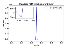
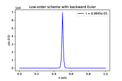
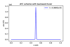
Figure 5.2. Left: Approximation of standard FEM scheme. Right: Approximation of low order scheme. Bottom: Approximation of AFC scheme.

5.2. Convergence study of the stabilized schemes

Next, we consider the following two sets of initial conditions for (1.1). The first one is

(5.2) $$u_{0} =10\,e^{-10((x-0.5)^{2}+(y-0.5)^{2})}+5,$$

$$c_{0} =0,$$

where note that $\|u_{0}\|_{L_{1}}\approx 7.984<4\pi$. The second set is

(5.3) $$u_{0} =\sin(\pi x)^{2}\cos(\pi y)^{2},$$

$$c_{0} =0,$$

where note that $\|u_{0}\|_{L_{1}}\approx 0.25<4\pi$. Thus, the solution $u$ in both examples does not blow-up.

We consider again the non-stabilized scheme where we discretize in time (1.7) using the backward Euler method and the stabilized schemes given by (3.1)-(3.2). We consider a sequence of triangulations $\mathcal{T}_{h}$ as described above with $h_{0}=1/M$, $M=10,20,40,80$. The final time is chosen to be $T=0.01,$ and we choose $k=\frac{1}{20}\,h_{0}$ for the computation of the error in $H^{1}$ norm and $k=\frac{1}{2}\,h_{0}^{2},$ for the $L_{2}-$norm.

Since the exact solution of (1.1) is unknown, the underlying numerical reference solution for each numerical scheme was obtained with $M=160$ and small time step $k=10^{-5}.$

In Tables 1 and 2 we present the errors for $u$ for the standard finite element scheme and the stabilized schemes, obtained in $L_{2}$ and $H^{1}$ norm and the correponding approximate order of convergence for the initial conditions (5.2).

In Tables 3 and 4 we present the errors for $u$ for the standard finite element scheme and the stabilized schemes, obtained in $L_{2}$ and $H^{1}$ norm and the correponding approximate order of convergence for the initial conditions (5.3).

Table 1. $L_{2}-$norm error and convergence order for the initial conditions (5.2).

$h_{0}$	Stand. FE	Order	Low order	Order	AFC	Order
$1/10$	$0.048937$		$0.062132$		$0.061509$
$1/20$	$0.012516$	$2.1087$	$0.017938$	$1.9213$	$0.017752$	$1.9218$
$1/40$	$0.003074$	$2.0982$	$0.004609$	$2.0306$	$0.004563$	$2.0305$
$1/80$	$0.000695$	$2.1836$	$0.001086$	$2.1223$	$0.001078$	$2.1183$

Table 2. $H^{1}-$norm error and convergence order for the initial conditions (5.2).

$h_{0}$	Stand. FE	Order	Low order	Order	AFC	Order
$1/10$	$2.24825$		$2.38762$		$2.43951$
$1/20$	$1.14089$	$1.0491$	$1.17669$	$1.0943$	$1.20292$	$1.0943$
$1/40$	$0.56325$	$1.0550$	$0.57232$	$1.0773$	$0.58521$	$1.0773$
$1/80$	$0.25609$	$1.1575$	$0.25814$	$1.1575$	$0.26387$	$1.1693$

Table 3. $L_{2}-$norm error and convergence order for the initial conditions (5.3).

$h_{0}$	Stand. FE	Order	Low order	Order	AFC	Order
$1/10$	$0.0053569$		$0.0064803$		$0.0065026$
$1/20$	$0.0013783$	$2.0994$	$0.0019202$	$1.8811$	$0.0019318$	$1.8771$
$1/40$	$0.0003378$	$2.1017$	$0.0004957$	$2.0241$	$0.0005008$	$2.0219$
$1/80$	$0.0000752$	$2.2048$	$0.0001750$	$1.5291$	$0.0001925$	$1.4042$

Table 4. $H^{1}-$norm error and convergence order for the initial conditions (5.3).

$h_{0}$	Stand. FE	Order	Low order	Order	AFC	Order
$1/10$	$0.24975$		$0.26590$		$0.26601$
$1/20$	$0.12776$	$1.0366$	$0.13226$	$1.0800$	$0.13231$	$1.0801$
$1/40$	$0.06333$	$1.0489$	$0.06453$	$1.0726$	$0.06453$	$1.0732$
$1/80$	$0.02889$	$1.1527$	$0.02913$	$1.1681$	$0.02918$	$1.1656$

6. Conclusions

In this paper, we presented the finite element error analysis for the stabilized schemes presented in [25] and [24]. We discretize space using continuous piecewise linear finite elements and time by the backward Euler method. Under assumptions for the triangulation used for the space discretization and the size of the time step $k$, we showed that the resulting coupled non-linear schemes have a unique solution and also remain non-negative. Further, we showed that the resulting discrete solution remains bounded and derived error estimates in $L_{2}$ and $H^{1}-$norm in space. Numerical experiments in two dimensions were presented for both the standard FEM and stabilized schemes. In the numerical experiments, we do not observe any significant difference between the low-order scheme and the AFC scheme for the two initial conditions that we have studied.

Appendix A Proof of Lemma 3.3

Proof.

Since, only the surrounding nodes to $P_{i}$ contributes to the corresponding row of the matrix, let $P_{i}$ be an interior node where the patch which has non-zero support is depicted on the left of the Fig. 2.1. Notice that for $j=1,\dots,8,$ we have

$$\tau_{P_{ij}P_{i}} =\lambda\int_{supp[\phi_{P_{ij}},\phi_{P_{i}}]}(\nabla c_{h}\cdot\nabla\phi_{P_{ij}})\phi_{P_{i}}\,dx$$

$$=\frac{\lambda}{3}\sum_{K\in supp[\phi_{P_{ij}},\phi_{P_{i}}]}\int_{K}\nabla c_{h}\cdot\nabla\phi_{P_{ij}}\,dx,$$

where $c_{h}\in\mathcal{S}_{h}$ and therefore $c_{h}=\sum_{j=1}^{N}\zeta_{j}\phi_{j}.$ Let $K_{1}$ and $K_{2}$ two triangles such its intersection consists of edge $e$ with endpoints $A$ and $B,$ see Fig. 2.1. Let $\phi_{A}$ and $\phi_{B}$ the basis functions at nodes $A$ and $B,$ respectively. Draganescu et al. [10] have given a closed formula for the computation of following integrals,

(A.1) $$\int_{K_{1}}\nabla\phi_{A}\cdot\nabla\phi_{B}\,dx =-\frac{\cot\gamma}{2},$$

(A.2) $$\int_{K_{1}}|\nabla\phi_{A}|^{2}\,dx =\frac{\sin\alpha}{2\sin\beta\,\sin\gamma},$$

(A.3) $$\int_{K_{1}\cup K_{2}}\nabla\phi_{A}\cdot\nabla\phi_{B}\,dx =-\frac{\sin(\gamma+\delta)}{2\sin\gamma\,\sin\delta}.$$

To prove the lemma, we need to distinguish the position of node $P_{i}$ in case of internal node and boundary node. Assume that $P_{i}$ is an internal node, with surrounding nodes as depicted in patch $\Pi_{0}$ of Fig. A.1.

Figure A.1. Left: The patch $\Pi_{0}$ around node $P_{i}.$ Right: The patch $\Pi_{1}$ around boundary node $P_{i}.$

Our goal is to prove that

(A.4) $$\sum_{j=0}^{8}\tau_{P_{ij}P_{i}}=\tau_{P_{i}P_{i}}+\tau_{P_{i1}P_{i}}+\dots+\tau_{P_{i8}P_{i}}=0,$$

where $P_{i0}:=P_{i}$ and

$$\tau_{P_{ij}P_{i}}=\frac{\lambda}{3}\sum_{l=1}^{N}\zeta_{P_{l}}\sum_{K\in supp[\phi_{P_{ij}},\phi_{P_{i}},\phi_{P_{l}}]}\int_{K}\nabla\phi_{P_{l}}\cdot\nabla\phi_{P_{ij}}\,dx,\text{ for }j=0,\dots,8.$$

The sum (A.4), can be written as

$$\sum_{j=0}^{8}\tau_{P_{ij}P_{i}}=\frac{\lambda}{3}\sum_{l=0}^{8}\zeta_{P_{il}}A_{l},$$

with $A_{l},$ $l=0,\dots,8$ are sum of integrals. We need to prove that $A_{l}=0,$ $l=0,\dots,8.$ We have,

$$A_{0}:=\int_{\text{supp}[P_{i}]}|\nabla\phi_{P_{i}}|^{2}\,dx+\sum_{l=1}^{8}\int_{K_{l}\cup K_{l+1}}\nabla\phi_{P_{i}}\cdot\nabla\phi_{P_{i,l+1}}\,dx,$$

and for $l=1,\dots,8,$

(A.5) $$A_{l+1} :=\int_{K_{l}\cup K_{l+1}}(|\nabla\phi_{P_{i,l+1}}|^{2}+\nabla\phi_{P_{i,l+1}}\cdot\nabla\phi_{P_{i}})\,dx$$

$$+\int_{K_{l}}\nabla\phi_{P_{i,l+1}}\cdot\nabla\phi_{P_{i,l}}\,dx+\int_{K_{l+1}}\nabla\phi_{P_{i,l+1}}\cdot\nabla\phi_{P_{i,l+2}}\,dx,$$

where $A_{9}:=A_{1}$ and with $P_{i9}=P_{i1}$, $P_{i10}=P_{i2}$, $K_{9}=K_{1}$, $K_{10}=K_{2}$. Using (A.1), (A.2) and (A.3), we get $A_{l}=0$, $l=0,\dots,8$. We work similar when $P_{i}$ is a boundary node. ∎

References

- [1] Baba, K., and Tabata, T. On a conservative upwind finite-element scheme for convective diffusion equations. RAIRO Anal 15 (1981), 3–25.
- [2] Barrenechea, G. R., Burman, E., and Karakatsani, F. Edge-based nonlinear diffusion for finite element approximations of convection-diffusion equations and its relation to algebraic flux-correction schemes. Numerische Mathematik 135 (2017), 521–545.
- [3] Barrenechea, G. R., John, V., and Knobloch, P. Analysis of algebraic flux correction schemes. SIAM J. Numer. Anal 54 (2016), 2427–2451.
- [4] Brenner, S. C., and Scott, L. R. The Mathematical Theory of Finite Element Methods, second ed. Springer, New York, 2008.
- [5] Chatzipantelidis, P., Lazarov, R., and Thomee, V. Some error estimates for the lumped mass finite element method for a parabolic problem. Mathematics of Computation 81 (2012), 1–20.
- [6] Chertock, A., Epshteyn, Y., Hu, H., and Kurganov, A. High-order positivity-preserving hybrid finite-volume-finite-difference methods for chemotaxis systems. Adv. Comput. Math. 44 (2018), 327–350.
- [7] Chertock, A., and Kurganov, A. A second-order positivity preserving central-upwind scheme for chemotaxis and haptotaxis models. Numer. Math. 111 (2008), 169–205.
- [8] Chertock, A., and Kurganov, A. High-resolution positivity and asymptotic preserving numerical methods for chemotaxis and related models. In Active particles, Volume 2. Advances in theory, models, and applications. Birkhäuser, Cham, 2019, pp. 109–148.
- [9] Ciarlet, P. G. The Finite Element Method for Elliptic Problems. Society for Industrial and Applied Mathematics, North-Holland, 2002.
- [10] Draganescu, A., Dupont, T. F., and Scott, L. R. Failure of the discrete maximum principle for an elliptic finite element problem. Math. Comp 74 (2004), 1–23.
- [11] Epshteyn, Y., and Izmirlioglu, A. Fully discrete analysis of a discontinuous finite element method for the keller-segel chemotaxis model. J. Sci. Comput. 40 (2009), 211–256.
- [12] Epshteyn, Y., and Kurganov, A. New interior penalty discontinuous galerkin methods for the keller-segel chemotaxis model. SIAM J. Numer. Anal 47 (2008), 386–408.
- [13] Filbet, F. A finite volume scheme for the patlak-keller-segel chemotaxis model. Numer. Math 104 (2006), 457–488.
- [14] Hillen, T., and Painter, K. J. A user’s guide to pde models for chemotaxis. J. Math. Biol. 58 (2009), 183–217.
- [15] Horstmann, D. From 1970 until present: the keller-segel model in chemotaxis and its con sequences i. Jahresber. Deutsch. Math.-Verein. 105 (2003), 103–165.
- [16] Horstmann, D. From 1970 until present: the keller-segel model in chemotaxis and its con sequences ii. Jahresber. Deutsch. Math.-Verein. 106 (2004), 51–89.
- [17] Keller, E. F., and Segel, L. A. Initiation of slime mold aggregation viewed as an instability. Journal of Theoretical Biology 26, 3 (1970), 399–415.
- [18] Kuzmin, D. A Guide to Numerical Methods for Transport Equations. University Erlangen-Nuremberg, Nuremberg, 2010.
- [19] Li, X. H., Shu, C.-W., and Yang, Y. Local discontinuous galerkin method for the keller-segel chemotaxis model. Journal of Scientific Computing 73, 2 (2017), 943–967.
- [20] Liu, J.-G., Wang, L., and Zhou, Z. Positivity-preserving and asymptotic preserving method for 2d keller-segal equations. Math. Comp. 87 (2018), 1165–1189.
- [21] Nagai, T., Senba, T., and Yoshida, K. Application of the trudinger-moser inequality to a parabolic system of chemotaxis. Funkcial Ekvac. 40 (1997), 411–433.
- [22] Perthame, B. Transport Equations in Biology. Frontiers in Math. Birkhauser Verlag, Basel, 2007.
- [23] Saito, N. Error analysis of a conservative finite-element approximation for the keller-segel system of chemotaxis. Commun. Pure Appl. Anal 11 (2012), 339–364.
- [24] Strehl, R. Advanced numerical treatment of chemotaxis-driven pdes in mathematical biology. PhD thesis, Technical University of Dortmund, PHD thesis, 2013.
- [25] Strehl, R., Sokolov, A., Kuzmin, D., and Turek, S. A flux-corrected finite element method for chemotaxis problems. Comput. Methods Appl. Math 10 (2010), 219–232.
- [26] Suzuki, T. Free Energy and Self-Interacting Particles. Birkhauser, Boston, 2005.
- [27] Tadmor, E. A review of numerical methods for nonlinear partial differential equations. Bull. Amer. Math. Soc. 49, 4 (2012), 507–554.