The Nearest Neutron Star Candidate in a Binary Revealed by Optical Time-domain Surveys

Abstract

The near-Earth (within $\sim 100$ pc) supernova explosions [e.g., 1; 2] in the past several million years can cause the global deposition of radioactive elements (e.g., ⁶⁰Fe) on Earth. The remnants of such supernovae are too old to be easily identified. It is therefore of great interest to search for million-year-old near-Earth neutron stars or black holes, the products of supernovae. However, neutron stars and black holes are challenging to find even in our Solar neighbourhood if they are not radio pulsars or X-ray/$\gamma$-ray emitters. Here we report the discovery of one of the nearest ($127.7\pm 0.3$ pc) neutron star candidates in a detached single-lined spectroscopic binary LAMOST J235456.73+335625.9 (hereafter J2354). Utilizing the time-resolved ground-based spectroscopy and space photometry, we find that J2354 hosts an unseen compact object with $M_{\mathrm{inv}}$ being $1.4\sim 1.6\ M_{\odot}$. The follow-up Swift ultraviolet (UV) and X-ray observations suggest that the UV and X-ray emission is produced by the visible star rather than the compact object. Hence, J2354 probably harbours a neutron star rather than a hot ultramassive white dwarf. Two-hour exceptionally sensitive radio follow-up observations with Five-hundred-meter Aperture Spherical radio Telescope fail to reveal any pulsating radio signals at the $6\sigma$ flux upper limit of $12.5\ \mu\mathrm{Jy}$. Therefore, the neutron star candidate in J2354 can only be revealed via our time-resolved observations. Interestingly, the distance between J2354 and our Earth can be as close as $\sim 50$ pc around $2.5$ Myrs ago, as revealed by the Gaia kinematics. Our discovery demonstrates a promising way to unveil the hidden near-Earth neutron stars in binaries by exploring the optical time domain, thereby facilitating understanding of the metal-enrichment history in our Solar neighbourhood.

97.60.Jd, 97.80.-d, 97.10.Cv

1 Introduction

As one of the most remarkable explosions, nearby supernovae can have great impacts on our Earth and other planets in the Solar system. Heavy elements produced by the supernova progenitors spread out because of the powerful supernova shocks and sink to the surfaces of Earth and other planets. Indeed, the radioactive elements (e.g., ⁶⁰Fe) from supernovae in the past million years are detected in Earth’s deep sea [e.g., 2]. Intensive $\gamma$-ray photons or cosmic rays emitted by the nearby supernovae may cause disastrous changes to Earth’s ecosystem and lead to catastrophic extinction events. Hence, the demographics of near-Earth neutron stars and black holes, the possible “fossils” of aforementioned supernovae, is of great importance to various research fields.

Traditional neutron-star searching methods often aim to detect radio pulsars, X-ray or $\gamma$-ray emitters [e.g., 3]. The majority of inactive neutron stars in our Solar neighborhood remain to be discovered. Optical time-domain surveys act as a supplementary method for hunting neutron stars in binaries by measuring the radial velocities ($V_{\mathrm{r}}$), the masses ($M_{\mathrm{vis}}$) of the visible companions, and the orbital periods ($P_{\mathrm{orb}}$). This approach has been proven successful in finding several stellar black holes [e.g., 4; 5; 6; 7; 8; 9; 10; 11; 12], albeit some candidates might be controversial [13], and is expected to substantially increase the sample size of non-interacting black hole binaries [14; 15; 16; 17]. The same methodology should also be efficient in discovering neutron stars.

To date, only a few neutron star candidates are discovered [e.g., 18; 19; 20; 21; 22; 23; 24] via time-resolved observations. These candidates are far from our Solar system ($\geq 300$ pc). By comparison, the nearest pulsar, PSR J0437-4715, locates only $156.8\pm 0.25$ pc away [25]. The distance of the nearest neutron star, RX J185635-3754 [26], which is identified by its thermal X-ray emission, is $123^{+11}_{-15}$ pc [27]. Neutron stars in X-ray binaries are often identified via type I X-ray bursts. Among them, Cen X-4 is the nearest one with a rather large distance of $1$ kpc [28]. X-ray faint or radio-quiet neutron stars in our Solar neighborhood ($\lesssim 150$ pc) remain to be discovered.

The Large Sky Area Multi-Object Fiber Spectroscopic Telescope (LAMOST) medium-resolution (MRS) time-domain survey is conducting repeated spectroscopic observations since October 2018 [29; 30]. The spectra from the LAMOST time-domain survey (with a spectral resolution of $R\approx 7500$) cover the wavelength ranges in [4950 Å, 5350 Å] and [6300 Å, 6800 Å] for the blue and red arms [31; 32], respectively.

We aim to find nearby binaries that harbour unseen neutron stars or black holes by exploring the LAMOST medium-resolution time-domain spectroscopic surveys. Our selection criteria are as follows.

• with more than three repeated high signal-to-noise (S/N $\geq 10$) LAMOST observations.

• are not classified as eclipsing binaries.

• with radial-velocity variations $\Delta V_{\mathrm{r}}\geq 80\ \mathrm{km\ s^{-1}}$ (i.e., like host a massive companion).

• close to our Earth.

Among the $\sim 2\times 10^{5}$ stars with the LAMOST medium-resolution time-domain spectroscopic coverage, J2354 is extraordinary because of its unusually large radial-velocity ($V_{\mathrm{r}}$) variations ($\lvert\Delta V_{\mathrm{r}}\rvert\simeq 400\ \mathrm{km\ s^{-1}}$) and small distance [33] to Earth ($127.7\pm 0.3$ pc). A systematic study of its archival and follow-up observations suggest that J2354 hosts a neutron star candidate. If confirmed, the neutron star is the nearest one detected in binaries. The supernova that produces the neutron star may significantly alter the Solar environment.

The manuscript is formatted as follows. In Section 2, we present the multi-band, multi-epoch spectroscopic, and photometric observations of J2354. In Section 3, we provide doppler spectroscopy evidence that J2354 harbours a neutron star candidate. In Section 4, we present our efforts to detect radio, X-ray, and $\gamma$-ray signatures of the neutron star candidate. Summary and future prospects are made in Section 5.

2 Data and Methodology

2.1 The Optical Spectroscopic Observations

2.1.1 The LAMOST Spectra

J2354 has the optical position of RA=358.736516 deg and DEC=33.940474 deg (J2000.0 coordinates) and its LAMOST spectra are consistent with a single-lined K7 dwarf star whose V-band magnitude is $13.61\pm 0.02$ mag. The single-lined spectroscopic binary (Figure 1) has 22 medium-resolution spectra in LAMOST Data Releases 8 and 9 (hereafter LDR8 and LDR9). Additional low-resolution (LRS; $R\approx 1800$) spectroscopic observations are obtained from the LAMOST Data Release 7 (hereafter LDR7); the spectra cover the wavelength ranges in [3690 Å, 9100 Å].

Absorption lines in J2354 LAMOST spectra show consistent large Doppler shifts; in fact, the spectra obtained in the same night can reach a maximum of $\sim 230\ \mathrm{km\ s^{-1}}$ (see Table 1).

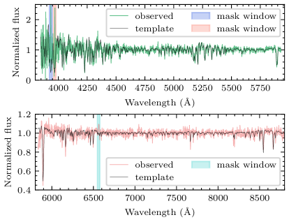
Figure 1: A LAMOST spectrum for the blue (upper panel) and red arms (lower panel) for J2354. The best-matching spectral template is shown in black. In the red arm, there is an evident H$\alpha$ emission line, and this line is masked during the radial-velocity measurements.

2.1.2 The CFHT Spectra

We requested two CFHT (Canada France Hawaii Telescope) follow-up observations on August 16, 2022, to obtain the high-resolution optical spectra of J2354. The purpose of the CFHT observations is twofold: to obtain accurate radial velocities and to determine the rotational broadening velocity $V_{\mathrm{rot}}\sin i$ of the visible star, where $V_{\mathrm{rot}}$ and $i$ are the star’s rotation velocity and the inclination angle, respectively. Hence, we took two on-target 20-minute exposures using the ESPaDOnS instrument in the “object+sky” spectroscopic mode. The wavelength coverage is from $3690$ to $10480$ $\mathrm{\AA}$ and the spectral resolution is $\sim 68000$. The two exposures were carefully arranged near the 0.75 quadrature phase of the visible star. As a result, during the two exposures, the “acceleration” of the radial velocity is minimized and only makes negligible contributions ($\sim 1\ \mathrm{km\ s^{-1}}$) to the observed line broadening.

The CFHT spectra are reduced with the OPERA (https://www.cfht.hawaii.edu/en/projects/opera/index.php) automatic pipeline developed by the CFHT data processing team. Cosmic rays contaminate some pixels of the reduced spectra. We use the conventional 3-sigma clipping to remove cosmic rays.

2.1.3 Measuring the Radial Velocities

The radial velocities of J2354 are measured via the standard cross-correlation function (CCF) method. The procedures can be briefly described as follows. First, PyHammer (PyHammer link), a Python tool to quickly and automatically classify stellar spectra [36; 37; 38] by comparing the observed spectra with templates, are used to determine the best-matching spectral type of the visible star in J2354 (see Figure 1). Second, the following wavelength window, [4910 Å, 5375 Å], is selected to normalize the LAMOST continuum spectra; note that cosmic rays are rejected via the median filter method. The best-matching K7 template is normalized via our spectool (https://gitee.com/zzxihep/spectool) package. Third, the standard CCF technique is applied to the LAMOST/CFHT spectra and our selected templates to measure the radial velocities. The radial-velocity uncertainties are estimated via the popular “flux randomization/random subset sampling (FR/RSS)” method [39], which randomizes the observed spectra via the following two steps: first, random subsets of the observed spectra are selected by adopting the bootstrapping method; second, Gaussian white random noise (whose standard deviations are fixed to the observed flux uncertainties) are added to the fluxes of the random subsets.

Table 1: The LAMOST and CFHT observation log

Spectrograph	HJD	Phase	RV(absorption lines)	RV(${\mathrm{H\alpha}}$)
	day		$\mathrm{km\ s^{-1}}$	$\mathrm{km\ s^{-1}}$
(1)	(2)	(3)	(4)	(5)
LAMOST-MRS	2458822.94999	0.976	$73^{+1.5}_{-2.2}$	$73^{+2.2}_{-1.0}$
	2458822.96622	0.009	$25^{+2.2}_{-2.2}$	$43^{+6.2}_{-2.3}$
	2458822.98244	0.043	$-20^{+2.2}_{-2.3}$	$-10^{+20.3}_{-9.1}$
	2458823.04789	0.180	$-159^{+1.5}_{-1.4}$	$-158^{+6.2}_{-6.2}$
	2458825.93698	0.200	$-168^{+1.0}_{-1.0}$	$-169^{+6.2}_{-3.2}$
	2458825.95118	0.229	$-173^{+1.0}_{-5.2}$	$-178^{+6.2}_{-3.2}$
	2458825.98035	0.290	$-173^{+5.2}_{-1.0}$	$-165^{+14.3}_{-7.2}$
	2458831.94381	0.716	$255^{+1.0}_{-1.0}$	$236^{+8.1}_{-5.1}$
	2458831.96003	0.750	$260^{+1.0}_{-1.0}$	$250^{+6.2}_{-6.2}$
	2458831.97625	0.783	$255^{+1.0}_{-1.0}$	$256^{+6.2}_{-6.2}$
	2458831.99264	0.818	$240^{+1.0}_{-1.0}$	$237^{+1.0}_{-1.0}$
	2458832.00885	0.851	$214^{+5.2}_{-1.0}$	$213^{+6.2}_{-1.0}$
	2459130.11192	0.003	$35^{+2.2}_{-1.4}$	$43^{+4.3}_{-4.3}$
	2459130.12845	0.037	$-14^{+1.4}_{-1.4}$	$-16^{+6.2}_{-3.2}$
	2459130.15552	0.094	$-85^{+1.5}_{-1.4}$	$-91^{+1.0}_{-1.0}$
	2459130.17179	0.128	$-117^{+1.4}_{-1.4}$	$-122^{+6.2}_{-6.2}$
	2459130.19079	0.167	$-151^{+2.3}_{-1.4}$	$-152^{+1.0}_{-1.0}$
	2459130.20705	0.201	$-168^{+1.4}_{-2.2}$	$-170^{+6.2}_{-1.0}$
	2459185.95841	0.369	$-120^{+3.4}_{-2.2}$	$-122^{+7.2}_{-4.2}$
	2459185.97463	0.403	$-83^{+2.2}_{-2.3}$	$-88^{+9.1}_{-5.1}$
	2459185.99087	0.437	$-41^{+3.2}_{-3.4}$	$-43^{+10.2}_{-5.3}$
	2459186.01184	0.481	$15^{+3.2}_{-3.4}$	$5^{+7.2}_{-4.2}$
LAMOST-LRS	2458101.95581	0.654	$225^{+3.2}_{-4.1}$	$206^{+32.7}_{-15.0}$
	2458101.96553	0.674	$237^{+5.1}_{-3.7}$	$231^{+34.7}_{-17.0}$
	2458101.97445	0.693	$243^{+4.1}_{-3.2}$	$237^{+33.7}_{-18.0}$
CFHT-ESPaDOnS	2459808.11664	0.750	$272^{+3.0}_{-3.0}$	—
	2459808.13110	0.780	$267^{+3.0}_{-3.0}$	—

We determine the radial velocities of absorption lines and the prominent H$\alpha$ emission line (in the following wavelength window [$6520$ Å, $6620$ Å]), respectively. The radial-velocity measurements are listed in Table 1.

2.1.4 Inferring the Rotational Broadening Velocity $V_{\mathrm{rot}}\sin i$

We can measure the rotational broadening velocity $V_{\mathrm{rot}}\sin i$ of the visible star from the CFHT spectra of the visible star. Note that the spectral resolution of the PyHammer template is too low to measure $V_{\mathrm{rot}}\sin i$. We determine the best-matching rotating template from the Marcs [40] theoretical atmospheric model. Our procedures are as follows. First, the radial velocities of the two CFHT spectra are measured with the aforementioned method. Note that the radial velocities are consistent with the LAMOST measurements at the same orbital phases. Second, the two CFHT spectra are shifted to have zero radial velocity with respect to the Marcs best-matching models and co-added to increase the signal-to-noise ratio. Third, we generate the Marcs spectra with $T_{\rm eff}=4100$ K and $\log{g}=4.66$ (see Section 2.4), but different $[\mathrm{Fe/H}]$, from $-1.0$ to $0.1$ in a $0.1$ step size. These Marcs spectra are downgraded to the spectral resolution of $R=68,000$. Fourth, the best-fit template is determined by minimizing $\chi^{2}=\sum(f_{\mathrm{o,\lambda}}-f_{\mathrm{m,\lambda}})^{2}/\sigma^{2}_{\mathrm{o,\lambda}}$, where $f_{\mathrm{o,\lambda}}$, $\sigma_{\mathrm{o,\lambda}}$, and $f_{\mathrm{m,\lambda}}$ are the co-added CFHT flux, flux uncertainty, and the Marcs model flux, respectively. The best-matching template has $[\mathrm{Fe/H}]=-0.3$.

We used the broadening function [41] to measure the $V_{\mathrm{rot}}\sin i$. The steps are as follows.

• Wavelength window selection. We choose three wavelength windows, each with 4–6 echelle orders, to measure $V_{\mathrm{rot}}\sin i$. The orders are: orders 50–45, orders 44–39, and orders 37–34, which cover three wavelength windows: 446.1–509.8 nm, 505.9–589.4 nm, and 559.8–667.5 nm, respectively. These orders contain many photospheric absorption lines and are free of telluric absorption lines. In addition, we mask Balmer emission lines. We use the average of the three best-fitting $V_{\mathrm{rot}}\sin i$ values from the three wavelength windows as our final $V_{\mathrm{rot}}\sin i$.

• Broadening function. We construct a design matrix $\hat{D}$ using the best-fit, non-broadened Marcs template, denoted as $T$ [41]. Each column of the $\hat{D}$ contains a continuum-normalized $T$ with a specific radial velocity $v$, spanning from $-$150 $\mathrm{km~{}s^{-1}}$ to 150 $\mathrm{km~{}s^{-1}}$. We aim to solve the equation $\hat{D}\vec{B}=\vec{O}$, where $\vec{B}$ and $\vec{O}$ are the unknown broadening function (BF) and the continuum-normalized, co-added CFHT spectrum. The singular value decomposition method is implemented [41] to solve the equation and constrain the BF.

• Rotational broadening. The spectral broadening contains the rotational broadening, the instrumental broadening ($\sim$4.4 $\mathrm{km~{}s^{-1}}$), and the broadening by macro-turbulence ($\simeq 2\ \mathrm{km\ s^{-1}}$). The latter two are small and negligible with respect to the rotational broadening. The $V_{\mathrm{rot}}\sin{i}$ is obtained by minimizing the $\chi^{2}$ between the calculated BF and the rotational profile [42, Equ. 18.14]:

  $$\begin{aligned} G(x)=&\frac{2(1-\epsilon)(1-x^{2})^{1/2}+\frac{\pi\epsilon}{2}(1-x^{2})}{\pi(1-\frac{\epsilon}{3})}&~{}\text{for}~{}\lvert x\rvert<1\\ &0&~{}\text{for}~{}\lvert x\rvert>1\\ \end{aligned}\,,$$ (1)

  where $x=V/(V_{\mathrm{rot}}\sin{i})$ and $V$ and $\epsilon$ are the shift velocity due to rotation and the limb-darkening coefficient, respectively. For the limb-darkening coefficient, we consider two cases: first, the limb-darkening coefficient for the absorption lines is zero; second, the limb-darkening coefficient is the same as for the continuum [as given by 43; 44]. The real case is probably somewhere between the two extremes [45]. The best-fitting result is shown in Figures 2 and 3.

• Uncertainty estimation. We use the Monte Carlo simulation to estimate the uncertainty of $V_{\mathrm{rot}}\sin{i}$. The best-fitting broadened Marcs template is randomly perturbed according to the observational flux uncertainties. We measure the mock $V_{\mathrm{rot}}\sin{i}$ of the perturbed template. This process is repeated $5,000$ times. The 16th-percentile and the 84-percentile of the mock $V_{\mathrm{rot}}\sin{i}$ distribution are used as the lower and the upper error bars.

For the first case (i.e., the limb-darkening coefficient of the absorption lines is zero), $V_{\mathrm{rot}}\sin{i}=63^{+8}_{-6}\ \mathrm{km\ s^{-1}}$; for the second case (i.e., absorption lines and continua share the same limb-darkening coefficient) $V_{\mathrm{rot}}\sin{i}=68.37^{+0.06}_{-0.09}\ \mathrm{km\ s^{-1}}$.

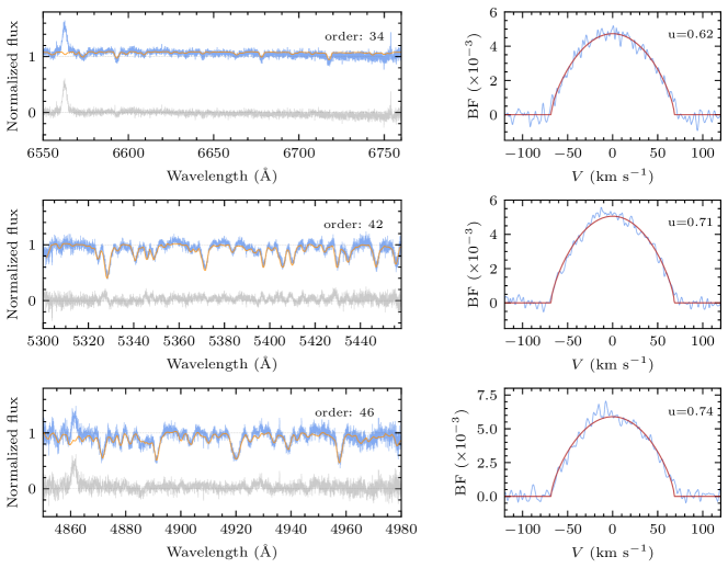
Figure 2: The CFHT spectra and rotational broadening measurements. Left panels: the co-added CFHT spectra (blue) at echelle orders 34 (top), 42 (middle), and 46 (bottom). These orders are selected from the three wavelength windows (see text), respectively. The best-fitting rotational-broadened Marcs template is shown in orange, and the residuals are shown in grey. The H$\alpha$ (6564 Å) and H$\beta$ (4863 Å) emission lines are clearly seen in orders 34 and 46, which are masked when measuring the $V_{\rm rot}\sin{i}$. Right panels: the three best-fitting broadening functions (blue) and rotational profiles (red) for the three wavelength windows.

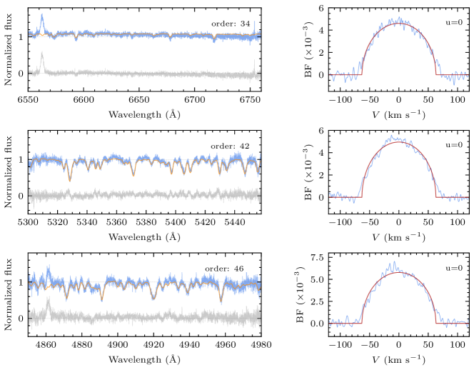
Figure 3: The same as Figure 2, but without limb darkening for absorption lines.

2.2 Optical-to-infrared light curves

J2354 has high-cadence (i.e., every 30 minutes) 30-day-long TESS full-frame images in Sector 17 [46; 47]. The TESS Sector 17 light curve is extracted and stored in STScI MAST (https://mast.stsci.edu/portal/Mashup/Clients/Mast/Portal.html). The STScI MAST PDC-SAPFLUX and its associate measurement errors (in units of $\mathrm{e^{-}\ s^{-1}}$) are used to construct the TESS light curve.

J2354 is also monitored by several ground-based time-domain surveys, namely, the All-Sky Automated Survey for Supernovae [ASAS-SN; 48] and the Zwicky Transient Facility [ZTF; 49]. The ASAS-SN light curve is retrieved from ASAS-SN Variable Stars Database (https://asas-sn.osu.edu/variables) and the corresponding cadence is $2\sim 3$ days; the ZTF $g$ and $r$ data are downloaded via IRSA (https://irsa.ipac.caltech.edu/cgi-bin/Gator/nph-scan?mission=irsa&submit=Select&projshort=ZTF) whose cadences are about $1$ day.

The Wide-field Infrared Survey Explorer [WISE; 50; 51] can provide WISE $W1$ and $W2$ infrared light curves for J2354; their cadences are $\sim 1.5$ days. We only consider observations with ccflags is 0; in this case, the target is unaffected by known artifacts.

2.3 X-ray and UV observations

We requested six Swift (the Neil Gehrels Swift Observatory) ToO observations (see Table 2) to investigate the possible X-ray and UV variability in J2354 (Target ID: $15376$) utilizing the X-ray Telescope (XRT) and Ultraviolet/Optical Telescope (UVOT).

We extract the Swift UVOT light curves via the uvmaghist tool in HEASoft version 6.30 (https://heasarc.gsfc.nasa.gov/docs/software/heasoft/). The source region is selected using a circle with a radius of $5$ arcsec centred on the optical position, and the corresponding background region is selected by an annulus with a $12.5$ arcsec inner radius and a $25.0$ arcsec outer radius.

X-ray observations, which were taken in the photon counting (PC) mode, show a low and highly variable count rate. We process the data with the packages available in HEASoft, and start with the standard data screening by using the task xrtpipeline. The source events are extracted from a circle of radius 15 pixels centred at the source position, having 26, 5, 13, 3, 1, and 3 photons (without background subtraction) for each individual observation. Hence, the X-ray emission of J2354 is highly variable and can only be detected in the first and third observations.

For two detections, we further extract the background spectra from a circular region of radius 30 pixels away from source. The ancillary response files are generated with the task xrtmkarf, and the response file (v014) from the CALDB database is adopted for the subsequent spectral analyses. The spectra are grouped to have at least 2 counts per bin, and they are analysed with xspec version 12.12.1 [52]. Because of limited photons, we fix the neutral hydrogen column density to the Galactic absorption ($5.65\times 10^{20}$ cm^-2) towards the direction of the source [53], and change the fit statistic to C-statistic. Fitting the spectra in 0.3–2.5 keV with an absorbed power-law model (tbabs*powerlaw in xspec), we obtain the best fitted parameters and their uncertainties in 90% confidence level as follows: for the first observation, the photon index $\Gamma=2.9_{-0.7}^{+0.8}$, the 0.3–2 keV unabsorbed flux $f=1.2_{-0.4}^{+0.6}\times 10^{-12}$ erg cm^-2 s^-1, and C-Statistic/dof$=9.0/10$; for the third observation, $\Gamma=2.7_{-2.6}^{+2.7}$, $f=3.4_{-2.2}^{+19.4}\times 10^{-13}$ erg cm^-2 s^-1, and C-Statistic/dof$=9.4/3$.

Table 2: The Swift observational log.

Epoch	Observation date	XRT mode	X-ray detection	UVOT mode	AFST (second)
(1)	(2)	(3)	(4)	(5)	(6)
1	2022-10-24	PC	Yes	0x30ed	1150
2	2022-11-02	PC	No	0x308f	1490
3	2022-11-06	PC	Yes	0x308f	1570
4	2022-11-12	PC	No	0x308f	440
5	2022-11-16	PC	No	0x308f	595
6	2022-11-19	PC	No	0x308f	755

Notes. AFST refers to the AS-Flown Science Timeline. Each of the first, second, and third observation consists of two or three separate exposures. The UVOT fluxes are independently measured in each exposure.

2.4 The UV-to-infrared spectral energy distribution

The multi-band (i.e., from UV to infrared) spectral energy distribution (SED) of J2354 is collected from GALEX [54; 55], the Sloan Digital Sky Survey [SDSS; 56], the AAVSO Photometric All-Sky Survey [APASS; 57], the Panoramic Survey Telescope and Rapid Response System [Pan-STARRS; 58; 59; 60; 61; 62], Gaia [33], TESS [47], the Two Micron All-Sky Survey [2MASS; 63; 64] and the Wide-field Infrared Survey Explorer [WISE; 50] (see Table 3).

We use the single-star model, ARIADNE (spectrAl eneRgy dIstribution bAyesian moDel averagiNg fittEr; https://github.com/jvines/astroARIADNE; [65]) to fit the observed optical-to-infrared SED and determine the model-free parameters: $T_{\mathrm{eff}}$, log $g$, [Fe/H], $D$, and $R$. Because of the close distance, a negligible extinction value of $A_{\rm{v}}=0.00^{+0.03}_{-0.00}$ mag is derived by using the colour excess $E(g-r)=0.00^{+0.01}_{-0.00}$ from 3D Dust Mapping (http://argonaut.skymaps.info/). As a result, the extinction value is fixed to be zero during the SED fitting. The prior distribution for the distance ($D$) is a normal distribution whose mean and standard deviation are fixed according to the Gaia result. The prior distribution for [Fe/H] is a normal distribution whose mean and standard deviation are $-0.3$ (Section 2.1.4) and 0.3, respectively. ARIADNE uses the stellar evolution model (isochrones) to resolve the parameter degeneracy. The adopted stellar synthetic SED models are Phoenix v2 (Phoenix v2 link), BT-Models (BT-Models link), Castelli & Kurucz (http://ssb.stsci.edu/cdbs/tarfiles/synphot3.tar.gz), and Kurucz 1993 (http://ssb.stsci.edu/cdbs/tarfiles/synphot4.tar.gz). ARIADNE uses nested sampling algorithms to estimate the best-fitting free parameters. Consistent with its single-lined nature, the best-fitting single-star SED model fits the observed optical-to-infrared data well (Figure 4).

Table 3: The multi-band SED.

Telescope	Band	$\lambda_{\rm central}$	magnitude	system	$\lambda f(\lambda)$	Ref.
		Å	mag		$\mathrm{\times 10^{-13}erg\ s^{-1}\ cm^{-2}}$
GALEX	NUV	2305	20.1 $\pm$ 0.14	AB	4.4 $\pm$ 0.59	[54; 55]
SDSS	u	3562	17.16 $\pm$ 0.01	AB	42 $\pm$ 0.38	[56]
	g	4719	14.974 $\pm$ 0.006	AB	236 $\pm$ 1.3	[56]
	r	6186	13.185 $\pm$ 0.003	AB	934 $\pm$ 2.6	[56]
	i	7500	12.767 $\pm$ 0.001	AB	1132 $\pm$ 1.0	[56]
	z	8961	12.932 $\pm$ 0.008	AB	816 $\pm$ 6.1	[56]
APASS	B	4348	14.9 $\pm$ 0.13	Vega	306.50 $\pm$ 37	[57]
	V	5505	13.61 $\pm$ 0.017	Vega	721 $\pm$ 11	[57]
Pan-STARRS	g	4866	14.036 $\pm$ 0.005	AB	545 $\pm$ 2.6	[58; 59; 62; 60; 61]
	y	9633	12.215 $\pm$ 0.001	AB	1474 $\pm$ 1.4	[58; 59; 62; 60; 61]
Gaia	BP	5129	13.792 $\pm$ 0.009	Vega	631 $\pm$ 5.2	[33]
	G	6425	13.037 $\pm$ 0.002	Vega	977 $\pm$ 1.8	[33]
	RP	7800	12.194 $\pm$ 0.006	Vega	1334 $\pm$ 7.4	[33]
TESS	red	7972	12.261 $\pm$ 0.008	Vega	1331 $\pm$ 9.8	[47]
2MASS	J	12408	11.06 $\pm$ 0.02	Vega	1452 $\pm$ 27	[63; 64]
	H	16514	10.45 $\pm$ 0.019	Vega	1235 $\pm$ 21	[63; 64]
	Ks	21656	10.32 $\pm$ 0.016	Vega	691 $\pm$ 10	[63; 64]
ALLWISE	W1	33792	10.24 $\pm$ 0.023	Vega	223 $\pm$ 4.7	[66]
	W2	46293	10.23 $\pm$ 0.02	Vega	91 $\pm$ 1.7	[66]
	W3	123340	10.06 $\pm$ 0.056	Vega	7.7 $\pm$ 0.4	[66]
	W4	222530	$>$ 8.89	Vega	$<$3.09	[66]

Notes. Photometric measurements with zero uncertainties or photometric flags (e.g., several Pan-STARRS bands) are excluded. Additional $4\%$ systematic uncertainties (i.e., the semi-amplitude of TESS flux variations) are added when performing the SED fitting.

ARIADNE uses nested sampling algorithms to obtain the posterior distributions of the free parameters. Hence, we obtain $T_{\mathrm{eff}}=4070^{+30}_{-40}$ K, $\log g=4.66\pm 0.02$ dex, radius $R=0.66^{+0.02}_{-0.01}\ R_{\odot}$ (see Figure 5), and the bolometric luminosity $L_{\mathrm{bol}}=4\pi R^{2}\sigma T_{\mathrm{eff}}^{4}=0.108\pm 0.005\ L_{\odot}$.

The stellar parameters are derived in different ways to check for consistency. First, the effective temperature $T_{\rm{eff}}=4171\pm 36$ K and $\log g=4.5\pm 0.12$ are reported in the LAMOST LDR8 database. Moreover, the $V$-band flux (13.61 mag) from UCAC4 [67], the Gaia distance (127.7 $\pm$ 0.3 pc), the extinction value $A_{\rm v}=0.00^{+0.03}_{-0.00}$ mag from 3D Dust Mapping, and the empirical bolometric correction [68] can be used to derive the bolometric luminosity $L_{\rm{bol}}=0.105\pm 0.008\,L_{\odot}$. The corresponding radius $R_{\mathrm{vis}}=\sqrt{L_{\rm{bol}}/(4\pi\sigma T_{\mathrm{eff}}^{4})}=0.62\pm 0.03\,R_{\odot}$. Second, as mentioned above, the tool ARIADNE can be used to fit the observed SED and infer the physical parameters of our source (see Figure 5). Third, we use the empirical relations of colour indexes and radius for main-sequence stars [69] to derive $R_{\mathrm{vis}}$, which is from $0.62\sim 0.65\ R_{\odot}$. The parameters from ARIADNE are broadly consistent with those from other methods.

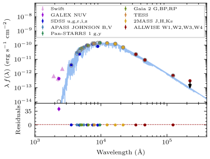
Figure 4: The SED fitting result. Upper: the best-fitting template (the blue curve) versus the observed SED (the filled dots). The grey open circles represent the model fluxes. The best-fitting stellar template (i.e., the blue curve) matches well with the observed optical SED. For the NUV band ($\lambda=2305$ Å) and the three Swift UV bands (UVW2, UVM2, UVW1), the stellar template fluxes are significantly dimmer than the observed ones. This NUV excess is due to the chromospheric activities, which are not taken into account when creating the stellar template. Lower: the ratios of the differences between the observed and model fluxes to the model fluxes. Note that the NUV, W3, and W4 fluxes are not considered during the SED fitting procedure. In addition, $4\%$ systematic uncertainties are added when fitting the SED.

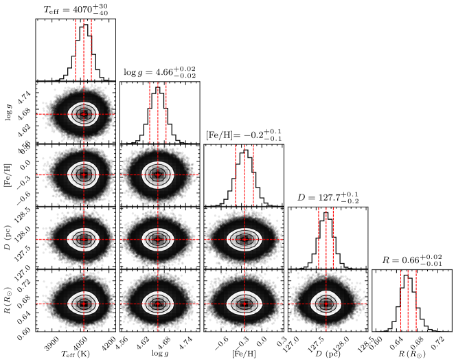
Figure 5: The posterior distributions of the stellar parameters derived from the ARIADNE SED fitting code. The dashed vertical lines indicate the 16th, 50th, and 84th percentiles of the distributions. The contours indicate the joint distributions of two parameters. Note that the ARIADNE SED fitting results are consistent with the values obtained from the LAMOST and Gaia databases.

3 Result

3.1 The Orbital Parameters and Ephemeris

The high-cadence (30 minutes) but short-duration ($\sim 30$ days) TESS light curve shows evident periodic signatures. We calculate the corresponding power spectral density (PSD) via the Lomb-Scargle algorithm [70]. Indeed, the Lomb-Scargle periodogram has two unequivocal peaks; the first and second peaks correspond to $P_{1}=0.23996$ days and $P_{2}=0.47991$ days, respectively. One of the two periodic signatures may be related to the orbital modulation.

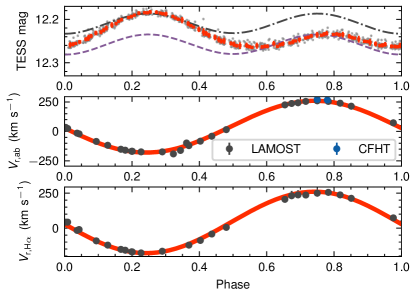
Figure 6: The phase-folded TESS light curve and radial velocities of J2354. Upper panel: the phase-folded (with $P_{\mathrm{orb}}=0.47992$ days) TESS light curves for J2354. The grey points and red squares correspond to the TESS observations in Sector 17 and its running mean over ten data points, respectively. The purple dashed and black dot-dashed curves represent the ellipsoidal-modulation light curves normalized according to the TESS magnitude at $\Phi=0.75$ and $\Phi=0.25$, respectively. The model parameters are $i=73$ degrees, $M_{\mathrm{vis}}=0.73\ M_{\odot}$, and $M_{\mathrm{inv}}=1.4\ M_{\odot}$. The TESS light curve shows additional variations beyond ellipsoidal modulations. Middle panel: the phase-folded LAMOST (black dots) and CFHT (blue dots) radial-velocity measurements of stellar absorption lines. The radial-velocity variations can be perfectly fitted by a sinusoidal function (the red curve), with the semi-amplitude $K_{\mathrm{vis}}=219.4\pm 0.5\ \mathrm{km\ s^{-1}}$. Lower panel: the phase-folded LAMOST H$\alpha$ radial velocities (black dots), which vary in tandem with the radial velocities of stellar absorption lines (the red curve). Hence, H$\alpha$ is produced by the chromospheric activity of the visible star. Note that the error bars of the data are small and invisible.

The orbital period can be further determined by fitting the radial-velocity variations. A Python code The Joker (https://github.com/adrn/thejoker; [71]), is used to fit a two-body system to the radial velocities (Figure 6). In the two-body system, the radial velocities are $V_{\mathrm{r}}(t)=\gamma+K(\cos(f+\omega)+e\cos(\omega))$, where $\gamma$, $K$, $f$, $\omega$, and $e$ represent the long-term mean barycentre velocity, the semi-amplitude, the true anomaly, the argument of periastron, and eccentricity, respectively. Note that the true anomaly $f$ is a function of $P_{\mathrm{orb}}$. An additional overall noise term ($s$) is allowed to account for the possible underestimation of the uncertainties of $V_{\mathrm{r}}$ [71]. We also assume that the LRS and MRS $V_{\mathrm{r}}$ measurements might have a small constant velocity offset ($dv_{0}$). The prior distribution for the standard deviation of the additional noise term $s$ is assumed to be a log-normal one (whose mean and standard deviation are $0.5\ \mathrm{km\ s^{-1}}$ and $1.5\ \mathrm{km\ s^{-1}}$, respectively). The prior distribution for $dv_{0}$ is a normal one (whose mean and standard deviation are $0\ \mathrm{km\ s^{-1}}$ and $5\ \mathrm{km\ s^{-1}}$). The prior distribution for $P_{\mathrm{orb}}$ is a uniform one in [$0.1$ days, $0.7$ days]. The prior distributions for $e$, $\omega$, $K$, and $\gamma$ are set to the default ones, i.e., a beta distribution for $e$, a uniform distribution for $\omega$, a normal distribution for $K$, and a normal distribution for $\gamma$, respectively. The Joker uses the MCMC algorithm to sample the posterior distributions of model parameters. The best-fitting $P_{\mathrm{orb}}$ is $0.47992$ days with the $1\sigma$ statistical uncertainty (the reported uncertainties always refer to the $1\sigma$ ranges, unless otherwise specified) of $10^{-5}$ days. The other period ($0.23996$ days) is incompatible with the radial-velocity variations. Hence, we conclude that the orbital period of J2354 is $P_{\mathrm{orb}}=0.47992$ days.

The ephemeris of the system is

$${\rm T}(\phi=0)=2459130.110499\,{\rm HJD}+0.47992\times N\ \,$$ (2)

where the phase $\phi=0$ corresponds to the visible star in the superior conjunction, and HJD is the Heliocentric Julian Date. Multi-band light curves from various telescopes can be phase-folded according to the same orbital ephemeris. The phase-folded light curves are asymmetric (Figure 6), driven by both ellipsoidal modulations (due to the tidal distortion of the visible star) and stellar activities (presumably due to e.g., starspots; for a detailed discussion, see Section 4.2). The ellipsoidal modulations account for the $P_{1}=0.23996$-day TESS PSD peak.

Other orbital parameters are determined by the radial-velocity fitting. For instance, The eccentricity $e=0.002\pm 0.002$, i.e., the orbit is nearly circular; the systematic velocity of J2354 is $\gamma=41^{+2.4}_{-2.3}\ \mathrm{km\ s^{-1}}$. The radial-velocity semi-amplitude of the absorption lines and the H$\alpha$ emission line are $K_{\mathrm{vis}}=219.4\pm 0.5\ \mathrm{km\ s^{-1}}$ and $K_{\mathrm{H\alpha}}=216\pm 2\ \mathrm{km\ s^{-1}}$. Hence, the mass function is $f(M_{\mathrm{inv}})=0.525\pm 0.004\ M_{\odot}$.

3.2 The Mass Function of the Compact Object

The mass function of the invisible object in the binary system is

$$f(M_{\rm{inv}})=(M_{\rm{inv}}\sin i)^{3}/(M_{\rm{vis}}+M_{\rm{inv}})^{2}=K_{\rm{vis}}^{3}P_{\rm{orb}}/(2\pi G)\ \,$$ (3)

where $M_{\rm{inv}}$, $M_{\rm{vis}}$, and $i$ are the mass of the invisible object, the mass of the visible star, and the inclination angle, respectively. According to the radial-velocity fitting results, the mass function of the invisible object in J2354 is $f(M_{\rm{inv}})=0.525\pm 0.004\ M_{\odot}$, which is also the lower limit for $M_{\rm{inv}}$.

Strong constraints on $M_{\rm{inv}}$ can be obtained if one knows $M_{\rm{vis}}$. We adopt $\log g$ and $R_{\mathrm{vis}}$ derived from ARIADNE to calculate $M_{\rm{vis}}$ and its uncertainty because $M_{\mathrm{vis}}^{g}=gR_{\mathrm{vis}}^{2}/G$ (where $G$ is the gravitational constant). Note that the ARIADNE code utilizes the stellar evolution model (isochrones) to significantly improve the constraint of $\log g$. Ten thousand realizations of $\log g$ and $R_{\mathrm{vis}}$ from the ARIADNE sampling results are used to construct the distribution of $M_{\rm{vis}}^{g}$. The median $M_{\mathrm{vis}}^{g}$ and its $1\sigma$ uncertainty (estimated via the 16th and 84th percentiles) are $0.73^{+0.06}_{-0.05}\ M_{\odot}$. Alternatively, the mass-luminosity relation [MLR; 72] and the observed absolute magnitudes in J, H, and K bands (see Table 3) can be used to estimate $M_{\mathrm{vis}}$; the resulting $M_{\mathrm{vis}}$ from the three bands are similar, i.e., $0.66_{-0.09}^{+0.11}\ M_{\odot}$. The MLR-based $M_{\mathrm{vis}}$ are statistically consistent (within $1\sigma$ uncertainties) with the SED-fitting $\log g$-based stellar mass. The SED-fitting $\log g$-based stellar mass and radius of J2354 is also statistically consistent with the empirical mass-radius relation for main sequence stars [69].

Given $f(M_{\rm{inv}})$ and $M_{\rm{vis}}$, $M_{\rm{inv}}$ anticorrelates with the inclination angle $i$. For the perfectly edge-on case (i.e., $i=90$ degrees), the corresponding mass of the invisible object is $1.29\pm 0.04\ M_{\odot}$. Hence, $M_{\rm{inv}}\geq 1.29\pm 0.04\ M_{\odot}$. If the unseen companion is a normal star, it would outshine the visible component. Hence, the unseen companion in J2354 ought to be a near-Earth compact object.

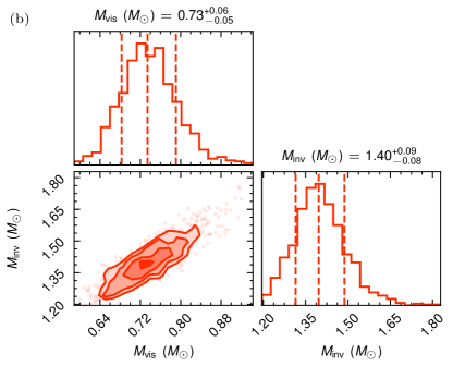
Figure 7: The joint probability density distribution (PDF) of the mass of the invisible object ($M_{\mathrm{inv}}$) versus that of the visible star ($M_{\mathrm{vis}}$). The left and right panels are for the limb darkening coefficient of absorption lines fixed to be zero and the continuum value, respectively. For each panel, the two histograms indicate the PDFs of $M_{\mathrm{inv}}$ and $M_{\mathrm{vis}}$; in each histogram, the three dashed vertical lines illustrate the $16$-th, $50$-th, and $84$-th percentiles of the distribution.

3.3 The Mass of the Compact Object

To determine $M_{\rm{inv}}$, we should estimate the inclination angle $i$. The rotational broadening velocity of the visible star, which is measured from the two high-resolution CFHT/ESPaDOnS spectra, depends upon the limb darkening coefficient of absorption lines: if the coefficient is zero (case I), $V_{\mathrm{rot}}\sin i=63^{+8}_{-6}\ \mathrm{km\ s^{-1}}$; if the coefficient is the same as for the continua (case II), $V_{\mathrm{rot}}\sin i=68.37^{+0.06}_{-0.09}\ \mathrm{km\ s^{-1}}$ (see Section 2.1.4). Due to the tidal synchronization, the spin period of the visible star should be identical to $P_{\mathrm{orb}}$. With such a rapid spin, the visible star is oblate. Hence, the equatorial plane $V_{\mathrm{rot}}$ should be evaluated numerically. We adopt Phoebe (PHysics Of Eclipsing BinariEs, which is publicly available from http://phoebe-project.org; [73]) to model $V_{\mathrm{rot}}$ of such a rapid spinning star. To do so, we set the Phoebe stellar parameters according to the ARIADNE posterior distributions of $M_{\mathrm{vis}}$ and $R_{\mathrm{vis}}$. Then, we use Phoebe to calculate the corresponding rotation spread functions for a star with a spin period of $0.47992$ days. Hence, we can obtain the distribution of the maximal rotation velocity of the visible star at the $\Phi=0.75$ phase. From the distribution, we have $V_{\mathrm{rot}}=71\pm 1.8\ \mathrm{km~{}s^{-1}}$. The corresponding inclination angle of J2354 is $i=62^{+3.0}_{-2.6}$ degrees (case I) or $i=73^{+5}_{-4}$ degrees (case II). Hence, as shown in Figure 7, $M_{\mathrm{inv}}=1.60^{+0.11}_{-0.10}\ M_{\odot}$ (case I) or $M_{\mathrm{inv}}=1.40^{+0.09}_{-0.08}\ M_{\odot}$ (case II). Some key physical properties of J2354 are summarized in Table 4.

The Roche lobe radius [74] of the visible star is $0.462(M_{\mathrm{vis}}/(M_{\mathrm{vis}}+M_{\mathrm{inv}}))^{(1/3)}a=1\ R_{\odot}$, where $a=3.2\ R_{\odot}$ is the semi-major axis of the binary. The corresponding Roche lobe fill factor is $65\%$, i.e., the Roche lobe is far from being filled by the visible star. If there was mass transferring from the visible star to the compact object, one would expect the Roche lobe filling factor to be as high as $90\%$ [75]. In summary, the birth mass of the unseen compact object is as large as $1.4\sim 1.6\ M_{\mathrm{\odot}}$. Given such a large birth mass, the compact object in J2354 is probably a neutron star. Although highly unlikely, the compact object might also be one of the most massive but cold white dwarfs within $\sim 100$ pc [76].

Table 4: A summary of the physical properties of J2354.

	Parameter	Value
Properties of the source
Right ascension	RA [deg]	358.736516
Declination	DEC [deg]	33.940474
V-band magnitude	[mag]	13.61$\pm$ 0.02
Distance	$D$ [pc]	127.7$\pm$ 0.3
Extinction	$A_{\rm V}$ [mag]	0.00${}^{+0.03}_{-0.00}$
Parameters of the visible star
Mass	$M_{\mathrm{vis}}^{g}$ [$M_{\odot}$]	0.73${}^{+0.06}_{-0.05}$
Radius	$R_{\mathrm{vis}}$ [$R_{\odot}$]	0.66${}^{+0.02}_{-0.01}$
Surface gravity	$\log g$ [cgs]	4.66$\pm$ 0.02
Effective temperature	$T_{\rm eff}$ [K]	4070${}^{+30}_{-40}$
Bolometric luminosity	$L_{\mathrm{bol}}$ [$L_{\odot}$]	0.108$\pm$ 0.005
Projected rotation velocity (case I)	$V_{\rm rot}\,\sin i$ [km s-1]	63${}^{+8}_{-6}$
Projected rotation velocity (case II)	$V_{\rm rot}\,\sin i$ [km s-1]	68.37${}^{+0.06}_{-0.09}$
Parameters of the orbit
Orbital period	$P_{\rm orb}$  [days]	0.47992$\pm$ 0.00001
Eccentricity	$e$	0.002$\pm$ 0.002
Center-of-mass $V_{\rm r}$	$\gamma$ [km s-1]	41${}^{+2.4}_{-2.3}$
$V_{\rm r}$ semi-amplitude of visible star	$K_{\mathrm{vis}}$ [km s-1]	219.4$\pm$0.5
$V_{\rm r}$ semi-amplitude of H$\alpha$	$K_{\mathrm{H_{\alpha}}}$ [km s-1]	216$\pm$2
Mass function	$f(M_{\mathrm{inv}})$ [$M_{\odot}$]	0.525$\pm$ 0.004
Inclination (case I)	$i\ [^{\circ}$]	62${}^{+3.0}_{-2.6}$
Inclination (case II)	$i\ [^{\circ}$]	73${}^{+5}_{-4}$
Minimum mass of the invisible object	$M_{\mathrm{inv,min}}$ [$M_{\odot}$]	1.29$\pm$ 0.04
Mass of the invisible object (case I)	$M_{\mathrm{inv}}$ [$M_{\odot}$]	1.60${}^{+0.11}_{-0.10}$
Mass of the invisible object (case II)	$M_{\mathrm{inv}}$ [$M_{\odot}$]	1.40${}^{+0.09}_{-0.08}$

Notes. The reported uncertainties correspond to $1\sigma$ confidence interval.

4 Discussion

4.1 The Origin of the UV Emission

As we showed in Section 2.4, the photometric emission of a K7 main sequence star matches the observed optical-to-infrared SED well (see Figure 4). However, the archival GALEX (Galaxy Evolution Explorer) NUV fluxes show clear excess beyond the photospheric emission. We argue that the NUV excess is produced by the chromospheric activity of the K7 star rather than the thermal emission from a white dwarf.

Six Swift follow-up ToO observations for J2354 are requested and cover various orbital phases (Section 2.3). In these observations, the compact object is not eclipsed by the K7 star. The average Swift $UVW1$, $UVM2$, and $UVW2$ also show clear excess beyond the photospheric emission. The UV flux excess in Swift $UVW1$, $UVM2$, and $UVW2$ and GALEX NUV bands can be obtained by subtracting the photosphere SED model from the observed UVW1, UVM2, and UVW2 fluxes. We then calculate the colours of the UV excess and compare it with the white dwarf templates of [77] with various temperature. To obtain the corresponding UV colours for each white dwarf template, we convolve the white dwarf templates of [77] with the UVOT filter response curves to obtain the corresponding UVOT synthetic photometries and colours. For all white dwarf templates, the synthetic UVOT colours are inconsistent with the observed ones (the left panel of Figure 8). We also compare the white dwarf templates of [77] with the SED of the UV excess (the right panel of Figure 8). The compact object cannot be a white dwarf that is hotter than $10^{4}$ K; otherwise, the corresponding UV fluxes are higher than that observed by Swift. The temperature upper limit is crucial for understanding the TESS variability and probing the physical nature of the compact object (see Section 4.2).

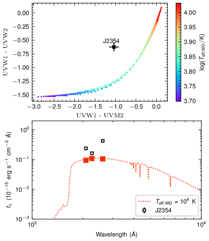
Figure 8: Comparison between the white dwarf templates and the UV excess. Upper: the UVW1$-$UVM2 colour vs the UVW1$-$UVW2 colour for the templates and J2354. Lower: the WD template with $T_{\mathrm{eff,WD}}=10,\ 000\ \mathrm{K}$ for a white dwarf with a radius of $0.005\ R_{\odot}$. The filled squares represent the template UVW2, UVW1, and UVM2 magnitudes by convolving the template with the filter response curves. The open squares are for the Swift UVOT observations. Note that the corresponding error bars are too small to be visible. Templates with effective temperatures $>10,\ 000$ K are inconsistent with the UVOT observations.

The UV excess with a GALEX NUV luminosity of $8\times 10^{29}\ \mathrm{erg\ s^{-1}}$ can be well explained by the chromospheric activities of the visible star. Indeed, J2354 shows a prominent H$\alpha$ emission line whose centre shifts in tandem with the stellar absorption features (Figure 6), and H$\alpha$ is a good indicator of chromospheric activities [78; 79]. The H$\alpha$ luminosities are measured by using the LDR8 and LDR9 spectra. To perform the flux calibration, the LAMOST spectra are compared with the SED in the wavelength range [6520 Å, 6620 Å], which covers H$\alpha$. Then, the H$\alpha$ flux can be simply measured as $f_{\mathrm{H}\alpha}=\int_{\mathrm{wl}}^{\mathrm{wr}}(f(\lambda)-\rm{c}(\lambda))d\lambda$, where wl and wr correspond to the left and right wings of the H$\alpha$ line, $f(\lambda)$ is the observed flux, and $\rm{c}(\lambda)$ is the flux of the underlying continuum. Note that the continuum flux is obtained by fitting a 5th-order polynomial to the spectra. The average (over the 22 spectra) H$\alpha$ flux is $\overline{f}_{\mathrm{H}\alpha}=2.63\times 10^{-14}\ \rm erg\ s^{-1}\ cm^{-2}$. Thus, the H$\alpha$ luminosity is $L_{\mathrm{H\alpha}}=4\pi D^{2}\overline{f}_{\mathrm{H\alpha}}=5.13\times 10^{28}\ \rm erg\ s^{-1}$, where $D=127.7$ pc. Following our previous work [21], we find that $L_{\mathrm{H\alpha}}/L_{\mathrm{bol}}$ and $L_{\mathrm{NUV}}/L_{\mathrm{bol}}$ of J2354 are comparable with isolated M dwarfs [78].

J2354 is undetected by the ROSAT all-sky surveys and lacks Chandra, XMM-Newton, or eROSITA public available data. In the first of our Swift follow-up observations, for the first time, we detect an X-ray counterpart in the optical position of J2354. This X-ray detection corresponds to an X-ray flare ($\log(L_{\mathrm{x,flare}}/[\mathrm{erg\ s^{-1}}])=30.3^{+0.2}_{-0.3}$) since the source is undetected in the following second, fourth, and fifth observations. In the third observation, the detected X-ray is also much less powerful than the first one (Section 2.3). If the X-ray flare is driven by the coronal activity of the visible star, one would also expect to detect a UV flare [80; 81]. Indeed, such a UV flare is observed in the UVOT exposures (Figure 9), with the UVM2 luminosity increasing by $L_{\mathrm{UVW2,flare}}\sim 3\pm 1.5\times 10^{29}\ \mathrm{erg\ s^{-1}}$. In summary, the X-ray and UV emission are produced by the coronal and chromospheric activities of the rapidly spinning visible star [82; 83].

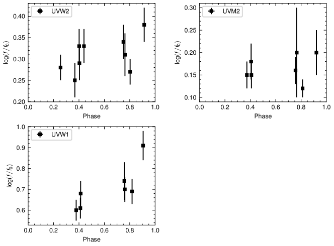
Figure 9: The UV fluxes as a function of the orbital phase of the visible star. Note that each Swift observation consists of $1\sim 3$ exposures, and the UV fluxes are independently measured in each exposure. Note that $f_{0}=10^{-15}\ \mathrm{erg\ s^{-1}\ cm^{-2}\ \AA^{-1}}$. In all observations, the compact object is not eclipsed by the visible companion. The UV emission shows evident variability, which is accompanied by an X-ray flare at the orbital phase $\phi\simeq 0.9$. Hence, the UV and X-ray emission is both produced by the visible star.

4.2 Possible origin of the orbital modulation

The optical variability of J2354 may offer new clues to the nature of the compact object. The model light curve of ellipsoidal modulations is calculated for $i=73$ degrees, $M_{\mathrm{vis}}=0.73\ M_{\odot}$, and $M_{\mathrm{inv}}=1.4\ M_{\odot}$ via ELLC [84]; the gravity-darkening is fixed to $0.44$ and adopt a quadratic limb-darkening law with the following parameters ($0.515$, $0.1754$) for the TESS band [44]. The model light curve can be normalized in two ways. That is, its median value is the same as the median of the TESS light curve at $\Phi=0.75$ (the purple dashed curve in Figure 6; hereafter the minor-peak model) or $\Phi=0.25$ (the black dot-dashed curve in Figure 6; hereafter the major-peak model). As shown in Figure 6, the model light curves can only account for the shape around one of the two peaks in the TESS light curve.

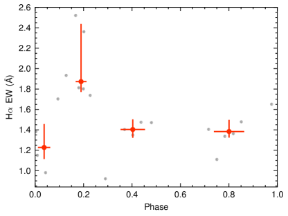
Figure 10: The Equivalent Width (EW) of the H$\alpha$ emission line at various phases. The gray dots represent the EW in each observation; the red circles with errorbars correspond to the averaged EWs and their $1\sigma$ uncertainties. The EW has a peak around $\Phi\simeq 0.25$.

To explain the full TESS light curve, non-uniform temperature distributions over the stellar surface should be introduced. For instance, the major-peak model with a giant starspot that is observable from $\Phi=0.4$ to $\Phi=1$ can resolve the discrepancy between the major-peak model and the TESS data. At these phases, strong magnetic fields in the starspots can induce strong photospheric activities. Hence, the $H\alpha$ EWs at these phases (from $\Phi=0.4$ to $\Phi=1$) are expected to be larger than those at other phases. This expectation is in contrast with observations (Figure 10). Alternatively, the minor-peak model with the additional heating from the companion also has the potential to explain the full TESS light curve. Indeed, the asymmetric TESS phase-folded light curve of J2354 are often observed in redback millisecond pulsars (e.g., PSR 3FGL J2039.6-5618 [85] and 3FGL J0212.1+5320 [86]) or detached magnetic white dwarfs [87]. The additional heating can be intra-binary shocks [e.g., 88] and is responsible for the major flux peak at $\Phi=0.25$. This speculation is further supported by the fact that the equivalent width (EW) of the $H\alpha$ emission line is strongest around $\Phi=0.25$. In summary, we find tentative evidence that the orbital modulations are driven by the additional heating, e.g., intra-binary shocks. A detailed comparison between the intra-binary shock model and the TESS light curves can constrain the shock properties [see, e.g., Figure 4 in 88], but is beyond the scope of this work.

The compact object in J2354 can only be a neutron star rather than a cold white dwarf if there is indeed additional heating. A cold white dwarf with $T_{\mathrm{eff,WD}}\lesssim 10^{4}$ K cannot drive strong winds; its thermal radiation to the surface of the visible star is about $\sigma_{\mathrm{SB}}T_{\mathrm{eff,WD}}^{4}(R_{\mathrm{WD}}/a_{\mathrm{orb}})^{2}(4\pi R_{\mathrm{vis}}^{2})\lesssim 10^{-4}L_{\odot}$, which is clearly too small to heat up the visible star. Instead, a neutron star can easily have a powerful and variable pulsar wind to significantly heat the visible star [e.g., 89]. In addition, J2354’s $M_{\mathrm{inv}}$ and $P_{\mathrm{orb}}$ are similar to several redbacks in [85]. In contrast, none of cool and massive WDs in [87] hosts a visible star as massive as that in J2354 (Figure 11).

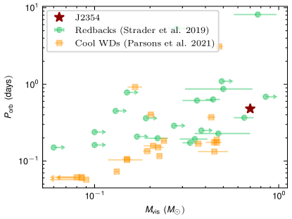
Figure 11: The orbital period vs the mass of the visible star. The orange squares are for cool but massive WDs in [87]; the green circles represent the redbacks in [85]; symbols with arrows correspond to the $1\sigma$ uncertainties. The mass of the visible star in J2354 is similar to redbacks rather than cool and massive WDs.

4.3 Searching for radio and $\gamma$-ray counterparts

We performed a total of 1.7 hours of targeted exceptionally sensitive radio follow-up observation for the pulsar search using FAST in the following three sessions: (1) 5 Sep 2021 17:30:00 to 18:30:00 UTC (Coordinated Universal Time); (2) 30 Aug 2022 17:55:00 to 18:15:00 UTC; (3) 25 Sep 2022 16:20:00 to 16:40:00 UTC. The orbital-phase ranges of the visible star in these sessions are [$0.20$, $0.28$], [$0.20$, $0.22$], and [$0.24$, $0.26$]. In these phases, the unseen compact object is not “shielded” by the K7 star. The first one minute and the last one minute were the calibration signal injection time for the flux and polarization calibration in each of the observations. Observations taken at FAST are using the centre beam of the 19-beams L-band receiver, the frequency range is $1.05$–$1.45$ GHz with the average system temperature 25 K [90]. Observational data are recorded in pulsar search mode, stored in PSRFITS format [91]. We performed two types of data processing during the observational campaign:

I. Dedicated and blind search:

Based on the Galactic electron density model of NE2001 [92] and YMW16 [93], we estimate, for the distance $D$=127.7 $\pm$ 0.3 pc, the corresponding with a dispersion measure (DM) of $\sim$ 1.4 pc cm^-3, and the line of sight maximal Galactic $\mathrm{DM_{max}}=50\ \mathrm{pc\ cm^{-3}}$. Meanwhile, the X-ray column density is fixed at $\mathrm{N_{H}}=5\times 10^{20}\ \mathrm{cm^{-2}}$ corresponding with $\mathrm{DM}\simeq 20\ \mathrm{pc\ cm^{-3}}$ estimated by the empirical linear relation [94]. Due to the model dependence and for the sake of robustness, we created de-dispersed time series for each pseudo-pointing over a range of DMs, from $0$–$300\ \mathrm{pc\ cm^{-3}}$, which is a factor of six larger than $\mathrm{DM_{max}}$. For each of the trial DMs, we searched for a periodical signal and first two order acceleration in the power spectrum based on the PRESTO [95] pipeline [96]. We checked all the pulsar candidates of signal-to-noise ratios (SNR) $>$ 6 and removed the narrowband radio frequency interferences (RFIs).

Both the periodical radio pulsations and single-pulse blind searches were performed for each observing epoch, but resulted in non-detections for all sessions. In Figure 12, we estimated the FAST detected sensitivity dependence of DMs and pulse duty cycle based on the radiometer equation. Furthermore, we calibrated the noise level of the baseline, and then measured the amount of pulsed flux above the baseline, giving the 6$\sigma$ upper limit of flux density measurement of 25 $\pm$ 5 $\mu$Jy in session (1) for persistent radio pulsations (assuming a pulse duty cycle of $0.05$–$0.3$). The time interval between sessions (2) and (3) is nearly one month, and the effect of interstellar scintillation can be well excluded; the upper limit of the flux density can be given for the average of the two measurements of 12.5 $\pm$ 2.0 $\mu$Jy in session (2-3).

II. Single pulse search:

The above search strategy was continued to be used to de-disperse the time series for single pulse search and flux calibration. We used PRESTO and HEIMDALL [https://sourceforge.net/p/heimdall-astro/wiki/Home/; 97] software. A zero-DM matched filter was applied to mitigate RFI in the blind search. All possible candidates were plotted, then be confirmed as RFIs by manual check. No pulsed radio emission with a dispersive signature was detected with an SNR $>6$. The upper limit of pulsed radio emission is $\sim 0.015$ Jy ms assuming a 1 ms wide burst in terms of integrated flux (fluence).

In summary, radio pulsars or persistent radio emission are not detected in the FAST data. The $6\sigma$ upper limit of the potential pulse power at $1.4$ GHz is therefore $<3.4\times 10^{23}\ \mathrm{erg\ s^{-1}}$. Unlike redbacks, J2354 also lacks $\gamma$-ray counterparts in the Fermi’s 4FGL catalogue [98]. Hence, the candidate is likely to be a non-beaming neutron star. Such sources will be easily missed in radio or $\gamma$-ray observations and can only be unearthed by optical time-domain surveys.

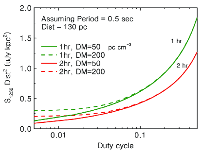
Figure 12: The sensitivity limits of 6$\sigma$ detection at 1250MHz vs. pulse duty cycle (assuming a young pulsar rotation period $\sim$0.5 second). The green and red curves are for the upper limit of flux densities with one-hour and two-hour integration time, respectively. The solid and dashed lines represent the sensitivity for DM = 50 pc cm^-3 and 200 pc cm^-3, respectively. For a nearby pulsar, the effective width $W_{\mathrm{eff}}\sim\sqrt{W^{2}_{\mathrm{int}}+\tau^{2}_{\mathrm{smear}}}$, and the inter-channel DM smearing time could be estimated by $\tau_{\mathrm{smear}}=8.3\mathrm{DM}(\delta f/\mathrm{MHz})/(f/\mathrm{GHz})^{3}\ \mu s$, where $\delta f=0.122\ \mathrm{MHz}$ is the frequency channel width. The detected pulse profile will be broadened due to that the inter-channel DM smearing, thus affecting the duty cycle. As a result, the sensitivity limit depends weakly upon DM, if a small duty cycle is assumed.

4.4 The Trajectory of J2354.

The distribution of the local ISM shows a bubble structure (i.e., the Local Bubble). The tridimensional map of the local ISM can be constructed from the inversion of the dust and gas absorption via the STructuring by Inversion the Local Interstellar Medium (hereafter Stilism; https://stilism.obspm.fr/) project [99]. In this map, the position of our Sun is $x,y,z=0$ pc, where $z$ is perpendicular to the galactic plane. The $xy$-plane (i.e., the galactic plane with $z=0$ pc), $xz$-plane (with $y=0$ pc), and $yz$-plane (with $x=0$ pc) cuts of the “Stilism” map are shown in Figure 13. It is evident that our Solar system and J2354 reside in the Local Bubble (Figure 13). The bubble is speculated to be created by multiple nearby supernovae [100; 101]. The possible remnants, neutron stars or black holes, of these supernovae remain hidden.

With the Gaia DR3 [33] proper-motion data ($23.21\pm 0.02\ \mathrm{mas\ yr^{-1}}$ and $-18.93\pm 0.01\ \mathrm{mas\ yr^{-1}}$ in the RA and DEC directions) and our best-fitting systematic radial-velocity (i.e., $\gamma=41\ \mathrm{km\ s^{-1}}$) for J2354, the trajectory of J2354 in our Galaxy in the past five Myrs can be calculated by considering the influence of the Milky-Way potential. The Milky Way potential consists of four components, i.e., a spherical nucleus, a bulge, a disk model [102] and a Navarro-Frenk-White halo. The trajectory is integrated backwards with a time step of $0.05$ Myrs via the Gala [103] code. We also calculate the three Galactic space velocities, i.e., $U$ (the velocity towards the Galactic centre), $V$ (the velocity along the Galactic rotation), and $W$ (the velocity in the direction of the North Galactic Pole). Then, we find that, according to the $UVW$ velocities [104], J2354 belongs to the Galactic thin disk.

The historical distances between J2354 and our Sun in the past $5$ Myrs are closer than the present distance, and the minimum historical distance is only $52$ pc (i.e., two times smaller than its present distance). Hence, the neutron star candidate in J2354 is one of the nearest neutron stars in binaries. Then, we calculate the trajectory of J2354 in the three cuts of the “Stilism” map. In the past five Myrs, J2354 has passed through the Local Bubble. The detection of J2354 demonstrates the possibility of improving the demographics of near-Earth supernovae in the era of time-domain astronomy, which is vital for our understanding of the chemical enrichment history and the energy and gas recycling around the Solar system.

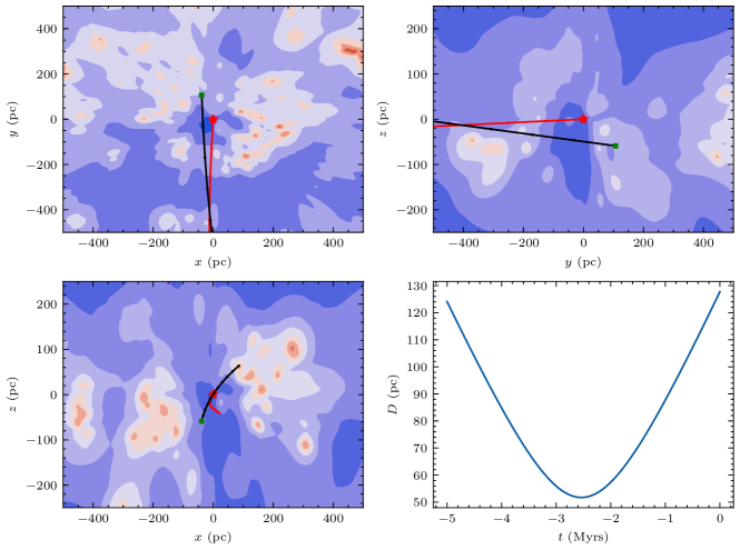
Figure 13: The current position (green squares) and the trajectory of J2354 in the past five Myrs (black dots and curve). The upper-left, upper-right, and lower-left are for the $xy$-plane, $yz$-plane, and $xz$-plane, respectively. The red star and curve indicate the current and historical positions of our Sun. The filled contours represent the “Stilism” tridimensional map of the local ISM [99]. The regions with low-density ISM are indicated as deep blue colours. The Local Bubble, a low-density cavity around our Sun, is evident in the figure. The lower-right panel shows the historical distance between J2354 and our Sun.

4.5 Alternative Scenario

We cannot entirely exclude the possibility that J2354 harbours an ultramassive but cold white dwarf. If so, the candidate in J2354 is one of the most massive nearby ($\lesssim 100$ pc) white dwarfs [76]. The other scenario involves a hierarchical triple system, i.e., the visible star orbits around two unseen $\sim 0.7\ M_{\odot}$ white dwarfs. According to the observed short orbital period and large mass function, the semi-major axis of the visible star’s orbit is only $a=3.2\ R_{\odot}$. For such a triple system to be stable, the semi-major axis of the orbit of the two unseen white dwarfs should be much smaller than the distance between the white dwarfs and the barycentre of J2354, which is $\sim 0.7/(0.7+1.4)a=1.1\ R_{\odot}$. The corresponding orbital period of the two white dwarfs is $\lesssim 10^{4}$ seconds. Then, the system is a promising gravitational wave source for space-based gravitational wave observatories [105; 106; 107]. We stress that, in the hierarchical triple system scenario, the two white dwarfs should also be cold ($\lesssim 10^{4}$ K). Hence, the additional heating from the white dwarfs is again too weak to explain the observed TESS light curve (see Section 4.2).

5 Summary

In this work, we have provided evidence that J2354 likely hosts a neutron star with a distance to Earth of $127.7\pm 0.3\ \mathrm{pc}$. Our results can be summarized as follows.

• We have used the doppler spectroscopy to measure the mass function of the unseen neutron star (Sections 2.1.1 & 3.2), i.e., $f(M_{\rm{inv}})=0.525\pm 0.004\ M_{\odot}$.

• We have determined the inclination angle of J2354 by measuring the rotational broadening velocity in the high-resolution CFHT spectra (Section 2.1.2). As a result, the mass of the neutron star candidate, $M_{\mathrm{inv}}=1.4\sim 1.6M_{\odot}$ (Section 3.3).

• We have, for the first time, detected the X-ray counterpart of J2354 via Swift. Our joint analyses of the Swift X-ray and UVOT variability suggest that the X-ray and UV emission are produced by the coronal and chromospheric activities of the K7 star (Section 4.1).

• Pulsating or persistent radio emission cannot be detected from the $1.7$-hour exceptionally sensitive FAST observations at the $6\sigma$ flux upper limit of $12.54\ \mathrm{\mu Jy}$ (Section 4.3).

• We have used the Gaia proper-motion measurements to calculate the historical positions of J2354 in the past five Myrs. It is evident that J2354 passes through the Local Bubble. The minimum distance between the Sun and J2354 is only $52$ pc (Section 4.4).

Acknowledgements. We thank Hong-Gang Yang, Yi-Han Song, Xuan Fang, Shuai Liu, and Yi-Ze Dong for beneficial discussions. W.M.G. acknowledges support from the National Key R&D Program of China under grant 2021YFA1600401, and the National Natural Science Foundation of China (NSFC) under grants 11925301 and 12033006. M.Y.S. acknowledges support from the NSFC under grants 11973002 and 12322303. Z.X.Z. acknowledges support from the NSFC under grant 12103041. J.F.L. acknowledges support from the NSFC under grants 11988101 and 11933004. P.W. acknowledges support from the NSFC under grant U2031117. J.F.Wang acknowledges support from the NSFC under grant 12033004. J.F.Wu acknowledges support from the NSFC under grant 12273029. W.M.G., J.F.Wang, and J.F.Wu acknowledge support from the NSFC under grant 12221003. J.Z. acknowledges support from the NSFC under grant 11933008. J.R.S. acknowledges support from the NSFC under grant 12090044. X.D.L. acknowledges support from the NSFC under grants 12041301 and 12121003.

This work uses the LAMOST spectra. Guoshoujing Telescope (the Large Sky Area Multi-Object Fiber Spectroscopic Telescope, LAMOST) is a National Major Scientific Project built by the Chinese Academy of Sciences. Funding for the project has been provided by the National Development and Reform Commission. LAMOST is operated and managed by the National Astronomical Observatories, Chinese Academy of Sciences. This work includes public data collected by the TESS mission, the NASA Galaxy Evolution Explorer (GALEX), SDSS, the Pan-STARRS1 Surveys (PS1), the Two Micron All Sky Survey(2MASS), the Wide-field Infrared Survey Explorer (WISE), the Zwicky Transient Facility (ZTF) project, ASAS-SN, the European Space Agency (ESA) mission Gaia, TESS, and the APASS database. This work uses data obtained through the Telescope Access Program (TAP), which has been funded by the TAP member institutes. This work made use of the data from FAST. FAST is a Chinese national mega-science facility, operated by National Astronomical Observatories, Chinese Academy of Sciences. This work uses data from Swift Target of Opportunity observations.

Conflict of interest. The authors declare that they have no conflict of interest.

References

- [1] J. Ellis, B. D. Fields, and D. N. Schramm, ApJ470, 1227 (1996), arXiv: astro-ph/9605128.
- [2] A. Wallner, M. B. Froehlich, M. A. C. Hotchkis, N. Kinoshita, M. Paul, M. Martschini, S. Pavetich, S. G. Tims, N. Kivel, D. Schumann, M. Honda, H. Matsuzaki, and T. Yamagata, Science 372, 742 (2021).
- [3] A. K. Harding, Frontiers of Physics 8, 679 (2013), arXiv: 1302.0869.
- [4] J. Casares, I. Negueruela, M. Ribó, I. Ribas, J. M. Paredes, A. Herrero, and S. Simón-Díaz, Nature505, 378 (2014), arXiv: 1401.3711.
- [5] J. Liu, H. Zhang, A. W. Howard, Z. Bai, Y. Lu, R. Soria, S. Justham, X. Li, Z. Zheng, T. Wang, K. Belczynski, J. Casares, W. Zhang, H. Yuan, Y. Dong, Y. Lei, H. Isaacson, S. Wang, Y. Bai, Y. Shao, Q. Gao, Y. Wang, Z. Niu, K. Cui, C. Zheng, X. Mu, L. Zhang, W. Wang, A. Heger, Z. Qi, S. Liao, M. Lattanzi, W.-M. Gu, J. Wang, J. Wu, L. Shao, R. Shen, X. Wang, J. Bregman, R. Di Stefano, Q. Liu, Z. Han, T. Zhang, H. Wang, J. Ren, J. Zhang, J. Zhang, X. Wang, A. Cabrera-Lavers, R. Corradi, R. Rebolo, Y. Zhao, G. Zhao, Y. Chu, and X. Cui, Nature575, 618 (2019), arXiv: 1911.11989.
- [6] T. A. Thompson, C. S. Kochanek, K. Z. Stanek, C. Badenes, R. S. Post, T. Jayasinghe, D. W. Latham, A. Bieryla, G. A. Esquerdo, P. Berlind, M. L. Calkins, J. Tayar, L. Lindegren, J. A. Johnson, T. W. S. Holoien, K. Auchettl, and K. Covey, Science 366, 637 (2019), arXiv: 1806.02751.
- [7] T. Jayasinghe, K. Z. Stanek, T. A. Thompson, C. S. Kochanek, D. M. Rowan, P. J. Vallely, K. G. Strassmeier, M. Weber, J. T. Hinkle, F. J. Hambsch, D. V. Martin, J. L. Prieto, T. Pessi, D. Huber, K. Auchettl, L. A. Lopez, I. Ilyin, C. Badenes, A. W. Howard, H. Isaacson, and S. J. Murphy, MNRAS504, 2577 (2021), arXiv: 2101.02212.
- [8] T. Shenar, H. Sana, L. Mahy, K. El-Badry, P. Marchant, N. Langer, C. Hawcroft, M. Fabry, K. Sen, L. A. Almeida, M. Abdul-Masih, J. Bodensteiner, P. A. Crowther, M. Gieles, M. Gromadzki, V. Hénault-Brunet, A. Herrero, A. d. Koter, P. Iwanek, S. Kozłowski, D. J. Lennon, J. M. Apellániz, P. Mróz, A. F. J. Moffat, A. Picco, P. Pietrukowicz, R. Poleski, K. Rybicki, F. R. N. Schneider, D. M. Skowron, J. Skowron, I. Soszyński, M. K. Szymański, S. Toonen, A. Udalski, K. Ulaczyk, J. S. Vink, and M. Wrona, Nature Astronomy 6, 1085 (2022), arXiv: 2207.07675.
- [9] S. Chakrabarti, J. D. Simon, P. A. Craig, H. Reggiani, T. D. Brandt, P. Guhathakurta, P. A. Dalba, E. N. Kirby, P. Chang, D. R. Hey, A. Savino, M. Geha, and I. B. Thompson, AJ166, 6 (2023), arXiv: 2210.05003.
- [10] K. El-Badry, H.-W. Rix, E. Quataert, A. W. Howard, H. Isaacson, J. Fuller, K. Hawkins, K. Breivik, K. W. K. Wong, A. C. Rodriguez, C. Conroy, S. Shahaf, T. Mazeh, F. Arenou, K. B. Burdge, D. Bashi, S. Faigler, D. R. Weisz, R. Seeburger, S. Almada Monter, and J. Wojno, MNRAS518, 1057 (2023), arXiv: 2209.06833.
- [11] K. El-Badry, H.-W. Rix, Y. Cendes, A. C. Rodriguez, C. Conroy, E. Quataert, K. Hawkins, E. Zari, M. Hobson, K. Breivik, A. Rau, E. Berger, S. Shahaf, R. Seeburger, K. B. Burdge, D. W. Latham, L. A. Buchhave, A. Bieryla, D. Bashi, T. Mazeh, and S. Faigler, MNRAS521, 4323 (2023), arXiv: 2302.07880.
- [12] A. Tanikawa, K. Hattori, N. Kawanaka, T. Kinugawa, M. Shikauchi, and D. Tsuna, ApJ946, 79 (2023), arXiv: 2209.05632.
- [13] M. Abdul-Masih, G. Banyard, J. Bodensteiner, E. Bordier, D. M. Bowman, K. Dsilva, M. Fabry, C. Hawcroft, L. Mahy, P. Marchant, G. Raskin, M. Reggiani, T. Shenar, A. Tkachenko, H. Van Winckel, L. Vermeylen, and H. Sana, Nature580, E11 (2020), arXiv: 1912.04092.
- [14] T. Yi, M. Sun, and W.-M. Gu, ApJ886, 97 (2019), arXiv: 1910.00822.
- [15] G. Wiktorowicz, Y. Lu, Ł. Wyrzykowski, H. Zhang, J. Liu, S. Justham, and K. Belczynski, ApJ905, 134 (2020), arXiv: 2006.08317.
- [16] H.-J. Mu, W.-M. Gu, T. Yi, L.-L. Zheng, H. Sou, Z.-R. Bai, H.-T. Zhang, Y.-J. Lei, and C.-M. Li, Science China Physics, Mechanics, and Astronomy 65, 229711 (2022), arXiv: 2209.14023.
- [17] H.-J. Mu, W.-M. Gu, T. Yi, L.-L. Zheng, H. Sou, Z.-R. Bai, H.-T. Zhang, Y.-J. Lei, and C.-M. Li, Science China Physics, Mechanics, and Astronomy 65, 109551 (2022).
- [18] J. J. Andrews, K. Taggart, and R. Foley, arXiv e-prints arXiv:2207.00680 (2022), arXiv: 2207.00680.
- [19] A. H. Knight, A. Ingram, M. Middleton, and J. Drake, MNRAS510, 4736 (2022), arXiv: 2201.02188.
- [20] T. Mazeh, S. Faigler, D. Bashi, S. Shahaf, N. Davidson, M. Green, R. Gomel, D. Maoz, A. Sussholz, S. Dong, H. Zhang, J. Liu, S. Wang, A. Luo, Z. Zheng, N. Hallakoun, V. Perdelwitz, D. W. Latham, I. Ribas, D. Baroch, J. C. Morales, E. Nagel, N. C. Santos, D. R. Ciardi, J. L. Christiansen, M. B. Lund, and J. N. Winn, MNRAS517, 4005 (2022), arXiv: 2206.11270.
- [21] T. Yi, W.-M. Gu, Z.-X. Zhang, L.-L. Zheng, M. Sun, J. Wang, Z. Bai, P. Wang, J. Wu, Y. Bai, S. Wang, H. Zhang, Y. Dong, Y. Shao, X.-D. Li, J. Zhang, Y. Huang, F. Yang, Q. Yu, H.-J. Mu, J.-B. Fu, S. Qi, J. Guo, X. Fang, C. Zheng, C.-Q. Li, J.-R. Shi, H. Chen, and J. Liu, Nature Astronomy 6, 1203 (2022), arXiv: 2209.12141.
- [22] H. Yuan, S. Wang, Z. Bai, Y. Wang, Y. Dong, M. Wang, S. Yu, Y. Zhao, Y. Chu, J. Liu, and H. Zhang, ApJ940, 165 (2022), arXiv: 2210.09987.
- [23] J. Lin, C. Li, W. Wang, H. Xu, J. Jiang, D. Yang, S. Yaqup, A. Iskanda, S. Ma, H. Niu, A. Esamdin, S. Liu, G. Ramsay, J. I. Vines, J. Shi, and R. Xu, ApJ944, L4 (2023), arXiv: 2210.11360.
- [24] S. Shahaf, D. Bashi, T. Mazeh, S. Faigler, F. Arenou, K. El-Badry, and H. W. Rix, MNRAS518, 2991 (2023), arXiv: 2209.00828.
- [25] D. J. Reardon, G. Hobbs, W. Coles, Y. Levin, M. J. Keith, M. Bailes, N. D. R. Bhat, S. Burke-Spolaor, S. Dai, M. Kerr, P. D. Lasky, R. N. Manchester, S. Osłowski, V. Ravi, R. M. Shannon, W. van Straten, L. Toomey, J. Wang, L. Wen, X. P. You, and X. J. Zhu, MNRAS455, 1751 (2016), arXiv: 1510.04434.
- [26] F. M. Walter, S. J. Wolk, and R. Neuhäuser, Nature379, 233 (1996).
- [27] F. M. Walter, T. Eisenbeiß, J. M. Lattimer, B. Kim, V. Hambaryan, and R. Neuhäuser, ApJ724, 669 (2010), arXiv: 1008.1709.
- [28] E. Kuulkers, J. J. M. in’t Zand, and J. P. Lasota, A&A503, 889 (2009), arXiv: 0809.3323.
- [29] C. Liu, J. Fu, J. Shi, H. Wu, Z. Han, L. Chen, S. Dong, Y. Zhao, J.-J. Chen, H. Zhang, Z.-R. Bai, X. Chen, W. Cui, B. Du, C.-H. Hsia, D.-K. Jiang, J. Hou, W. Hou, H. Li, J. Li, L. Li, J. Liu, J. Liu, A.-L. Luo, J.-J. Ren, H.-J. Tian, H. Tian, J.-X. Wang, C.-J. Wu, J.-W. Xie, H.-L. Yan, F. Yang, J. Yu, B. Zhang, H. Zhang, L.-Y. Zhang, W. Zhang, G. Zhao, J. Zhong, W. Zong, and F. Zuo, arXiv e-prints arXiv:2005.07210 (2020), arXiv: 2005.07210.
- [30] W. Zong, J.-N. Fu, P. De Cat, J. Wang, J. Shi, A. Luo, H. Zhang, A. Frasca, J. Molenda-Żakowicz, R. O. Gray, C. J. Corbally, G. Catanzaro, T. Cang, J. Wang, J. Chen, Y. Hou, J. Liu, H. Niu, Y. Pan, H. Tian, H. Yan, Y. Zhang, and H. Zuo, ApJS251, 15 (2020), arXiv: 2009.06843.
- [31] Y. Hou, L. Tang, M. Xu, H. Jiang, Z. Hu, L. Wang, H. Ji, and Y. Zhu, in Ground-based and Airborne Instrumentation for Astronomy VII, (edited by C. J. Evans, L. Simard, and H. Takami), volume 10702 of Society of Photo-Optical Instrumentation Engineers (SPIE) Conference Series, 107021I (2018).
- [32] B. Zhang, C. Liu, C.-Q. Li, L.-C. Deng, T.-S. Yan, and J.-R. Shi, Research in Astronomy and Astrophysics 20, 051 (2020), arXiv: 1910.13154.
- [33] Gaia Collaboration, A. Vallenari, A. G. A. Brown, T. Prusti, J. H. J. de Bruijne, F. Arenou, C. Babusiaux, M. Biermann, O. L. Creevey, C. Ducourant, D. W. Evans, L. Eyer, R. Guerra, A. Hutton, C. Jordi, S. A. Klioner, U. L. Lammers, L. Lindegren, X. Luri, F. Mignard, C. Panem, D. Pourbaix, S. Randich, P. Sartoretti, C. Soubiran, P. Tanga, N. A. Walton, C. A. L. Bailer-Jones, U. Bastian, R. Drimmel, F. Jansen, D. Katz, M. G. Lattanzi, F. van Leeuwen, J. Bakker, C. Cacciari, J. Castañeda, F. De Angeli, C. Fabricius, M. Fouesneau, Y. Frémat, L. Galluccio, A. Guerrier, U. Heiter, E. Masana, R. Messineo, N. Mowlavi, C. Nicolas, K. Nienartowicz, F. Pailler, P. Panuzzo, F. Riclet, W. Roux, G. M. Seabroke, R. Sordoørcit, F. Thévenin, G. Gracia-Abril, J. Portell, D. Teyssier, M. Altmann, R. Andrae, M. Audard, I. Bellas-Velidis, K. Benson, J. Berthier, R. Blomme, P. W. Burgess, D. Busonero, G. Busso, H. Cánovas, B. Carry, A. Cellino, N. Cheek, G. Clementini, Y. Damerdji, M. Davidson, P. de Teodoro, M. Nuñez Campos, L. Delchambre, A. Dell’Oro, P. Esquej, J. Fernández-Hernández, E. Fraile, D. Garabato, P. García-Lario, E. Gosset, R. Haigron, J. L. Halbwachs, N. C. Hambly, D. L. Harrison, J. Hernández, D. Hestroffer, S. T. Hodgkin, B. Holl, K. Janßen, G. Jevardat de Fombelle, S. Jordan, A. Krone-Martins, A. C. Lanzafame, W. Löffler, O. Marchal, P. M. Marrese, A. Moitinho, K. Muinonen, P. Osborne, E. Pancino, T. Pauwels, A. Recio-Blanco, C. Reylé, M. Riello, L. Rimoldini, T. Roegiers, J. Rybizki, L. M. Sarro, C. Siopis, M. Smith, A. Sozzetti, E. Utrilla, M. van Leeuwen, U. Abbas, P. Ábrahám, A. Abreu Aramburu, C. Aerts, J. J. Aguado, M. Ajaj, F. Aldea-Montero, G. Altavilla, M. A. Álvarez, J. Alves, F. Anders, R. I. Anderson, E. Anglada Varela, T. Antoja, D. Baines, S. G. Baker, L. Balaguer-Núñez, E. Balbinot, Z. Balog, C. Barache, D. Barbato, M. Barros, M. A. Barstow, S. Bartolomé, J. L. Bassilana, N. Bauchet, U. Becciani, M. Bellazzini, A. Berihuete, M. Bernet, S. Bertone, L. Bianchi, A. Binnenfeld, S. Blanco-Cuaresma, A. Blazere, T. Boch, A. Bombrun, D. Bossini, S. Bouquillon, A. Bragaglia, L. Bramante, E. Breedt, A. Bressan, N. Brouillet, E. Brugaletta, B. Bucciarelli, A. Burlacu, A. G. Butkevich, R. Buzzi, E. Caffau, R. Cancelliere, T. Cantat-Gaudin, R. Carballo, T. Carlucci, M. I. Carnerero, J. M. Carrasco, L. Casamiquela, M. Castellani, A. Castro-Ginard, L. Chaoul, P. Charlot, L. Chemin, V. Chiaramida, A. Chiavassa, N. Chornay, G. Comoretto, G. Contursi, W. J. Cooper, T. Cornez, S. Cowell, F. Crifo, M. Cropper, M. Crosta, C. Crowley, C. Dafonte, A. Dapergolas, M. David, P. David, P. de Laverny, F. De Luise, R. De March, J. De Ridder, R. de Souza, A. de Torres, E. F. del Peloso, E. del Pozo, M. Delbo, A. Delgado, J. B. Delisle, C. Demouchy, T. E. Dharmawardena, P. Di Matteo, S. Diakite, C. Diener, E. Distefano, C. Dolding, B. Edvardsson, H. Enke, C. Fabre, M. Fabrizio, S. Faigler, G. Fedorets, P. Fernique, A. Fienga, F. Figueras, Y. Fournier, C. Fouron, F. Fragkoudi, M. Gai, A. Garcia-Gutierrez, M. Garcia-Reinaldos, M. García-Torres, A. Garofalo, A. Gavel, P. Gavras, E. Gerlach, R. Geyer, P. Giacobbe, G. Gilmore, S. Girona, G. Giuffrida, R. Gomel, A. Gomez, J. González-Núñez, I. González-Santamaría, J. J. González-Vidal, M. Granvik, P. Guillout, J. Guiraud, R. Gutiérrez-Sánchez, L. P. Guy, D. Hatzidimitriou, M. Hauser, M. Haywood, A. Helmer, A. Helmi, M. H. Sarmiento, S. L. Hidalgo, T. Hilger, N. Hładczuk, D. Hobbs, G. Holland, H. E. Huckle, K. Jardine, G. Jasniewicz, A. Jean-Antoine Piccolo, Ó. Jiménez-Arranz, A. Jorissen, J. Juaristi Campillo, F. Julbe, L. Karbevska, P. Kervella, S. Khanna, M. Kontizas, G. Kordopatis, A. J. Korn, Á. Kóspál, Z. Kostrzewa-Rutkowska, K. Kruszyńska, M. Kun, P. Laizeau, S. Lambert, A. F. Lanza, Y. Lasne, J. F. Le Campion, Y. Lebreton, T. Lebzelter, S. Leccia, N. Leclerc, I. Lecoeur-Taibi, S. Liao, E. L. Licata, H. E. P. Lindstrøm, T. A. Lister, E. Livanou, A. Lobel, A. Lorca, C. Loup, P. Madrero Pardo, A. Magdaleno Romeo, S. Managau, R. G. Mann, M. Manteiga, J. M. Marchant, M. Marconi, J. Marcos, M. M. S. Marcos Santos, D. Marín Pina, S. Marinoni, F. Marocco, D. J. Marshall, L. M. Polo, J. M. Martín-Fleitas, G. Marton, N. Mary, A. Masip, D. Massari, A. Mastrobuono-Battisti, T. Mazeh, P. J. McMillan, S. Messina, D. Michalik, N. R. Millar, A. Mints, D. Molina, R. Molinaro, L. Molnár, G. Monari, M. Monguió, P. Montegriffo, A. Montero, R. Mor, A. Mora, R. Morbidelli, T. Morel, D. Morris, T. Muraveva, C. P. Murphy, I. Musella, Z. Nagy, L. Noval, F. Ocaña, A. Ogden, C. Ordenovic, J. O. Osinde, C. Pagani, I. Pagano, L. Palaversa, P. A. Palicio, L. Pallas-Quintela, A. Panahi, S. Payne-Wardenaar, X. Peñalosa Esteller, A. Penttilä, B. Pichon, A. M. Piersimoni, F. X. Pineau, E. Plachy, G. Plum, E. Poggio, A. Prša, L. Pulone, E. Racero, S. Ragaini, M. Rainer, C. M. Raiteri, N. Rambaux, P. Ramos, M. Ramos-Lerate, P. Re Fiorentin, S. Regibo, P. J. Richards, C. Rios Diaz, V. Ripepi, A. Riva, H. W. Rix, G. Rixon, N. Robichon, A. C. Robin, C. Robin, M. Roelens, H. R. O. Rogues, L. Rohrbasser, M. Romero-Gómez, N. Rowell, F. Royer, D. Ruz Mieres, K. A. Rybicki, G. Sadowski, A. Sáez Núñez, A. Sagristà Sellés, J. Sahlmann, E. Salguero, N. Samaras, V. Sanchez Gimenez, N. Sanna, R. Santoveña, M. Sarasso, M. Schultheis, E. Sciacca, M. Segol, J. C. Segovia, D. Ségransan, D. Semeux, S. Shahaf, H. I. Siddiqui, A. Siebert, L. Siltala, A. Silvelo, E. Slezak, I. Slezak, R. L. Smart, O. N. Snaith, E. Solano, F. Solitro, D. Souami, J. Souchay, A. Spagna, L. Spina, F. Spoto, I. A. Steele, H. Steidelmüller, C. A. Stephenson, M. Süveges, J. Surdej, L. Szabados, E. Szegedi-Elek, F. Taris, M. B. Taylo, R. Teixeira, L. Tolomei, N. Tonello, F. Torra, J. Torra, G. Torralba Elipe, M. Trabucchi, A. T. Tsounis, C. Turon, A. Ulla, N. Unger, M. V. Vaillant, E. van Dillen, W. van Reeven, O. Vanel, A. Vecchiato, Y. Viala, D. Vicente, S. Voutsinas, M. Weiler, T. Wevers, L. Wyrzykowski, A. Yoldas, P. Yvard, H. Zhao, J. Zorec, S. Zucker, and T. Zwitter, arXiv e-prints arXiv:2208.00211 (2022), arXiv: 2208.00211.
- [34] B. Kiziltan, A. Kottas, M. De Yoreo, and S. E. Thorsett, ApJ778, 66 (2013), arXiv: 1011.4291.
- [35] L. S. Rocha, R. R. A. Bachega, J. E. Horvath, and P. H. R. S. Moraes, arXiv e-prints arXiv:2107.08822 (2021), arXiv: 2107.08822.
- [36] A. Y. Kesseli, A. A. West, M. Veyette, B. Harrison, D. Feldman, and J. J. Bochanski, ApJS230, 16 (2017), arXiv: 1702.06957.
- [37] A. Kesseli, A. West, M. Veyette, B. Harrison, D. Feldman, D. Morgan, C. Theissen, and C. Robinson, PyHammer: Python spectral typing suite, Astrophysics Source Code Library, record ascl:2002.011 (2020), arXiv: 2002.011.
- [38] B. R. Roulston, P. J. Green, and A. Y. Kesseli, ApJS249, 34 (2020), arXiv: 2006.01199.
- [39] B. M. Peterson, I. Wanders, K. Horne, S. Collier, T. Alexander, S. Kaspi, and D. Maoz, PASP110, 660 (1998), arXiv: astro-ph/9802103.
- [40] B. Gustafsson, B. Edvardsson, K. Eriksson, U. G. Jørgensen, Å. Nordlund, and B. Plez, A&A486, 951 (2008), arXiv: 0805.0554.
- [41] S. M. Rucinski, AJ104, 1968 (1992).
- [42] D. F. Gray, The Observation and Analysis of Stellar Photospheres (2005).
- [43] A. Claret and S. Bloemen, A&A529, A75 (2011).
- [44] A. Claret, A&A600, A30 (2017), arXiv: 1804.10295.
- [45] T. Shahbaz, MNRAS339, 1031 (2003), arXiv: astro-ph/0211266.
- [46] G. R. Ricker, J. N. Winn, R. Vanderspek, D. W. Latham, G. Á. Bakos, J. L. Bean, Z. K. Berta-Thompson, T. M. Brown, L. Buchhave, N. R. Butler, R. P. Butler, W. J. Chaplin, D. Charbonneau, J. Christensen-Dalsgaard, M. Clampin, D. Deming, J. Doty, N. De Lee, C. Dressing, E. W. Dunham, M. Endl, F. Fressin, J. Ge, T. Henning, M. J. Holman, A. W. Howard, S. Ida, J. M. Jenkins, G. Jernigan, J. A. Johnson, L. Kaltenegger, N. Kawai, H. Kjeldsen, G. Laughlin, A. M. Levine, D. Lin, J. J. Lissauer, P. MacQueen, G. Marcy, P. R. McCullough, T. D. Morton, N. Narita, M. Paegert, E. Palle, F. Pepe, J. Pepper, A. Quirrenbach, S. A. Rinehart, D. Sasselov, B. Sato, S. Seager, A. Sozzetti, K. G. Stassun, P. Sullivan, A. Szentgyorgyi, G. Torres, S. Udry, and J. Villasenor, Journal of Astronomical Telescopes, Instruments, and Systems 1, 014003 (2015).
- [47] K. G. Stassun, R. J. Oelkers, M. Paegert, G. Torres, J. Pepper, N. De Lee, K. Collins, D. W. Latham, P. S. Muirhead, J. Chittidi, B. Rojas-Ayala, S. W. Fleming, M. E. Rose, P. Tenenbaum, E. B. Ting, S. R. Kane, T. Barclay, J. L. Bean, C. E. Brassuer, D. Charbonneau, J. Ge, J. J. Lissauer, A. W. Mann, B. McLean, S. Mullally, N. Narita, P. Plavchan, G. R. Ricker, D. Sasselov, S. Seager, S. Sharma, B. Shiao, A. Sozzetti, D. Stello, R. Vanderspek, G. Wallace, and J. N. Winn, AJ158, 138 (2019), arXiv: 1905.10694.
- [48] C. S. Kochanek, B. J. Shappee, K. Z. Stanek, T. W. S. Holoien, T. A. Thompson, J. L. Prieto, S. Dong, J. V. Shields, D. Will, C. Britt, D. Perzanowski, and G. Pojmański, PASP129, 104502 (2017), arXiv: 1706.07060.
- [49] F. J. Masci, R. R. Laher, B. Rusholme, D. L. Shupe, S. Groom, J. Surace, E. Jackson, S. Monkewitz, R. Beck, D. Flynn, S. Terek, W. Landry, E. Hacopians, V. Desai, J. Howell, T. Brooke, D. Imel, S. Wachter, Q.-Z. Ye, H.-W. Lin, S. B. Cenko, V. Cunningham, U. Rebbapragada, B. Bue, A. A. Miller, A. Mahabal, E. C. Bellm, M. T. Patterson, M. Jurić, V. Z. Golkhou, E. O. Ofek, R. Walters, M. Graham, M. M. Kasliwal, R. G. Dekany, T. Kupfer, K. Burdge, C. B. Cannella, T. Barlow, A. Van Sistine, M. Giomi, C. Fremling, N. Blagorodnova, D. Levitan, R. Riddle, R. M. Smith, G. Helou, T. A. Prince, and S. R. Kulkarni, PASP131, 018003 (2019), arXiv: 1902.01872.
- [50] E. L. Wright, P. R. M. Eisenhardt, A. K. Mainzer, M. E. Ressler, R. M. Cutri, T. Jarrett, J. D. Kirkpatrick, D. Padgett, R. S. McMillan, M. Skrutskie, S. A. Stanford, M. Cohen, R. G. Walker, J. C. Mather, D. Leisawitz, I. Gautier, Thomas N., I. McLean, D. Benford, C. J. Lonsdale, A. Blain, B. Mendez, W. R. Irace, V. Duval, F. Liu, D. Royer, I. Heinrichsen, J. Howard, M. Shannon, M. Kendall, A. L. Walsh, M. Larsen, J. G. Cardon, S. Schick, M. Schwalm, M. Abid, B. Fabinsky, L. Naes, and C.-W. Tsai, AJ140, 1868 (2010), arXiv: 1008.0031.
- [51] A. Mainzer, J. Bauer, R. M. Cutri, T. Grav, J. Masiero, R. Beck, P. Clarkson, T. Conrow, J. Dailey, P. Eisenhardt, B. Fabinsky, S. Fajardo-Acosta, J. Fowler, C. Gelino, C. Grillmair, I. Heinrichsen, M. Kendall, J. D. Kirkpatrick, F. Liu, F. Masci, H. McCallon, C. R. Nugent, M. Papin, E. Rice, D. Royer, T. Ryan, P. Sevilla, S. Sonnett, R. Stevenson, D. B. Thompson, S. Wheelock, D. Wiemer, M. Wittman, E. Wright, and L. Yan, ApJ792, 30 (2014), arXiv: 1406.6025.
- [52] K. A. Arnaud, in Astronomical Data Analysis Software and Systems V, (edited by G. H. Jacoby and J. Barnes), volume 101 of Astronomical Society of the Pacific Conference Series, 17 (1996).
- [53] HI4PI Collaboration, N. Ben Bekhti, L. Flöer, R. Keller, J. Kerp, D. Lenz, B. Winkel, J. Bailin, M. R. Calabretta, L. Dedes, H. A. Ford, B. K. Gibson, U. Haud, S. Janowiecki, P. M. W. Kalberla, F. J. Lockman, N. M. McClure-Griffiths, T. Murphy, H. Nakanishi, D. J. Pisano, and L. Staveley-Smith, A&A594, A116 (2016), arXiv: 1610.06175.
- [54] D. C. Martin, J. Fanson, D. Schiminovich, P. Morrissey, P. G. Friedman, T. A. Barlow, T. Conrow, R. Grange, P. N. Jelinsky, B. Milliard, O. H. W. Siegmund, L. Bianchi, Y.-I. Byun, J. Donas, K. Forster, T. M. Heckman, Y.-W. Lee, B. F. Madore, R. F. Malina, S. G. Neff, R. M. Rich, T. Small, F. Surber, A. S. Szalay, B. Welsh, and T. K. Wyder, ApJ619, L1 (2005), arXiv: astro-ph/0411302.
- [55] P. Morrissey, T. Conrow, T. A. Barlow, T. Small, M. Seibert, T. K. Wyder, T. Budavári, S. Arnouts, P. G. Friedman, K. Forster, D. C. Martin, S. G. Neff, D. Schiminovich, L. Bianchi, J. Donas, T. M. Heckman, Y.-W. Lee, B. F. Madore, B. Milliard, R. M. Rich, A. S. Szalay, B. Y. Welsh, and S. K. Yi, ApJS173, 682 (2007), arXiv: 0706.0755.
- [56] K. N. Abazajian, J. K. Adelman-McCarthy, M. A. Agüeros, S. S. Allam, C. Allende Prieto, D. An, K. S. J. Anderson, S. F. Anderson, J. Annis, N. A. Bahcall, C. A. L. Bailer-Jones, J. C. Barentine, B. A. Bassett, A. C. Becker, T. C. Beers, E. F. Bell, V. Belokurov, A. A. Berlind, E. F. Berman, M. Bernardi, S. J. Bickerton, D. Bizyaev, J. P. Blakeslee, M. R. Blanton, J. J. Bochanski, W. N. Boroski, H. J. Brewington, J. Brinchmann, J. Brinkmann, R. J. Brunner, T. Budavári, L. N. Carey, S. Carliles, M. A. Carr, F. J. Castander, D. Cinabro, A. J. Connolly, I. Csabai, C. E. Cunha, P. C. Czarapata, J. R. A. Davenport, E. de Haas, B. Dilday, M. Doi, D. J. Eisenstein, M. L. Evans, N. W. Evans, X. Fan, S. D. Friedman, J. A. Frieman, M. Fukugita, B. T. Gänsicke, E. Gates, B. Gillespie, G. Gilmore, B. Gonzalez, C. F. Gonzalez, E. K. Grebel, J. E. Gunn, Z. Györy, P. B. Hall, P. Harding, F. H. Harris, M. Harvanek, S. L. Hawley, J. J. E. Hayes, T. M. Heckman, J. S. Hendry, G. S. Hennessy, R. B. Hindsley, J. Hoblitt, C. J. Hogan, D. W. Hogg, J. A. Holtzman, J. B. Hyde, S.-i. Ichikawa, T. Ichikawa, M. Im, Ž. Ivezić, S. Jester, L. Jiang, J. A. Johnson, A. M. Jorgensen, M. Jurić, S. M. Kent, R. Kessler, S. J. Kleinman, G. R. Knapp, K. Konishi, R. G. Kron, J. Krzesinski, N. Kuropatkin, H. Lampeitl, S. Lebedeva, M. G. Lee, Y. S. Lee, R. French Leger, S. Lépine, N. Li, M. Lima, H. Lin, D. C. Long, C. P. Loomis, J. Loveday, R. H. Lupton, E. Magnier, O. Malanushenko, V. Malanushenko, R. Mandelbaum, B. Margon, J. P. Marriner, D. Martínez-Delgado, T. Matsubara, P. M. McGehee, T. A. McKay, A. Meiksin, H. L. Morrison, F. Mullally, J. A. Munn, T. Murphy, T. Nash, A. Nebot, J. Neilsen, Eric H., H. J. Newberg, P. R. Newman, R. C. Nichol, T. Nicinski, M. Nieto-Santisteban, A. Nitta, S. Okamura, D. J. Oravetz, J. P. Ostriker, R. Owen, N. Padmanabhan, K. Pan, C. Park, G. Pauls, J. Peoples, John, W. J. Percival, J. R. Pier, A. C. Pope, D. Pourbaix, P. A. Price, N. Purger, T. Quinn, M. J. Raddick, P. Re Fiorentin, G. T. Richards, M. W. Richmond, A. G. Riess, H.-W. Rix, C. M. Rockosi, M. Sako, D. J. Schlegel, D. P. Schneider, R.-D. Scholz, M. R. Schreiber, A. D. Schwope, U. Seljak, B. Sesar, E. Sheldon, K. Shimasaku, V. C. Sibley, A. E. Simmons, T. Sivarani, J. Allyn Smith, M. C. Smith, V. Smolčić, S. A. Snedden, A. Stebbins, M. Steinmetz, C. Stoughton, M. A. Strauss, M. SubbaRao, Y. Suto, A. S. Szalay, I. Szapudi, P. Szkody, M. Tanaka, M. Tegmark, L. F. A. Teodoro, A. R. Thakar, C. A. Tremonti, D. L. Tucker, A. Uomoto, D. E. Vanden Berk, J. Vandenberg, S. Vidrih, M. S. Vogeley, W. Voges, N. P. Vogt, Y. Wadadekar, S. Watters, D. H. Weinberg, A. A. West, S. D. M. White, B. C. Wilhite, A. C. Wonders, B. Yanny, D. R. Yocum, D. G. York, I. Zehavi, S. Zibetti, and D. B. Zucker, ApJS182, 543 (2009), arXiv: 0812.0649.
- [57] A. A. Henden, M. Templeton, D. Terrell, T. C. Smith, S. Levine, and D. Welch, VizieR Online Data Catalog II/336 (2016).
- [58] K. C. Chambers, E. A. Magnier, N. Metcalfe, H. A. Flewelling, M. E. Huber, C. Z. Waters, L. Denneau, P. W. Draper, D. Farrow, D. P. Finkbeiner, C. Holmberg, J. Koppenhoefer, P. A. Price, A. Rest, R. P. Saglia, E. F. Schlafly, S. J. Smartt, W. Sweeney, R. J. Wainscoat, W. S. Burgett, S. Chastel, T. Grav, J. N. Heasley, K. W. Hodapp, R. Jedicke, N. Kaiser, R. P. Kudritzki, G. A. Luppino, R. H. Lupton, D. G. Monet, J. S. Morgan, P. M. Onaka, B. Shiao, C. W. Stubbs, J. L. Tonry, R. White, E. Bañados, E. F. Bell, R. Bender, E. J. Bernard, M. Boegner, F. Boffi, M. T. Botticella, A. Calamida, S. Casertano, W. P. Chen, X. Chen, S. Cole, N. Deacon, C. Frenk, A. Fitzsimmons, S. Gezari, V. Gibbs, C. Goessl, T. Goggia, R. Gourgue, B. Goldman, P. Grant, E. K. Grebel, N. C. Hambly, G. Hasinger, A. F. Heavens, T. M. Heckman, R. Henderson, T. Henning, M. Holman, U. Hopp, W. H. Ip, S. Isani, M. Jackson, C. D. Keyes, A. M. Koekemoer, R. Kotak, D. Le, D. Liska, K. S. Long, J. R. Lucey, M. Liu, N. F. Martin, G. Masci, B. McLean, E. Mindel, P. Misra, E. Morganson, D. N. A. Murphy, A. Obaika, G. Narayan, M. A. Nieto-Santisteban, P. Norberg, J. A. Peacock, E. A. Pier, M. Postman, N. Primak, C. Rae, A. Rai, A. Riess, A. Riffeser, H. W. Rix, S. Röser, R. Russel, L. Rutz, E. Schilbach, A. S. B. Schultz, D. Scolnic, L. Strolger, A. Szalay, S. Seitz, E. Small, K. W. Smith, D. R. Soderblom, P. Taylor, R. Thomson, A. N. Taylor, A. R. Thakar, J. Thiel, D. Thilker, D. Unger, Y. Urata, J. Valenti, J. Wagner, T. Walder, F. Walter, S. P. Watters, S. Werner, W. M. Wood-Vasey, and R. Wyse, arXiv e-prints arXiv:1612.05560 (2016), arXiv: 1612.05560.
- [59] E. A. Magnier, K. C. Chambers, H. A. Flewelling, J. C. Hoblitt, M. E. Huber, P. A. Price, W. E. Sweeney, C. Z. Waters, L. Denneau, P. W. Draper, K. W. Hodapp, R. Jedicke, N. Kaiser, R. P. Kudritzki, N. Metcalfe, C. W. Stubbs, and R. J. Wainscoat, ApJS251, 3 (2020), arXiv: 1612.05240.
- [60] E. A. Magnier, W. E. Sweeney, K. C. Chambers, H. A. Flewelling, M. E. Huber, P. A. Price, C. Z. Waters, L. Denneau, P. W. Draper, D. Farrow, R. Jedicke, K. W. Hodapp, N. Kaiser, R. P. Kudritzki, N. Metcalfe, C. W. Stubbs, and R. J. Wainscoat, ApJS251, 5 (2020), arXiv: 1612.05244.
- [61] E. A. Magnier, E. F. Schlafly, D. P. Finkbeiner, J. L. Tonry, B. Goldman, S. Röser, E. Schilbach, S. Casertano, K. C. Chambers, H. A. Flewelling, M. E. Huber, P. A. Price, W. E. Sweeney, C. Z. Waters, L. Denneau, P. W. Draper, K. W. Hodapp, R. Jedicke, N. Kaiser, R. P. Kudritzki, N. Metcalfe, C. W. Stubbs, and R. J. Wainscoat, ApJS251, 6 (2020), arXiv: 1612.05242.
- [62] C. Z. Waters, E. A. Magnier, P. A. Price, K. C. Chambers, W. S. Burgett, P. W. Draper, H. A. Flewelling, K. W. Hodapp, M. E. Huber, R. Jedicke, N. Kaiser, R. P. Kudritzki, R. H. Lupton, N. Metcalfe, A. Rest, W. E. Sweeney, J. L. Tonry, R. J. Wainscoat, and W. M. Wood-Vasey, ApJS251, 4 (2020), arXiv: 1612.05245.
- [63] M. F. Skrutskie, R. M. Cutri, R. Stiening, M. D. Weinberg, S. Schneider, J. M. Carpenter, C. Beichman, R. Capps, T. Chester, J. Elias, J. Huchra, J. Liebert, C. Lonsdale, D. G. Monet, S. Price, P. Seitzer, T. Jarrett, J. D. Kirkpatrick, J. E. Gizis, E. Howard, T. Evans, J. Fowler, L. Fullmer, R. Hurt, R. Light, E. L. Kopan, K. A. Marsh, H. L. McCallon, R. Tam, S. Van Dyk, and S. Wheelock, AJ131, 1163 (2006).
- [64] R. M. Cutri, M. F. Skrutskie, S. van Dyk, C. A. Beichman, J. M. Carpenter, T. Chester, L. Cambresy, T. Evans, J. Fowler, J. Gizis, E. Howard, J. Huchra, T. Jarrett, E. L. Kopan, J. D. Kirkpatrick, R. M. Light, K. A. Marsh, H. McCallon, S. Schneider, R. Stiening, M. Sykes, M. Weinberg, W. A. Wheaton, S. Wheelock, and N. Zacarias, VizieR Online Data Catalog II/246 (2003).
- [65] J. I. Vines and J. S. Jenkins, MNRAS513, 2719 (2022), arXiv: 2204.03769.
- [66] R. M. Cutri, E. L. Wright, T. Conrow, J. W. Fowler, P. R. M. Eisenhardt, C. Grillmair, J. D. Kirkpatrick, F. Masci, H. L. McCallon, S. L. Wheelock, S. Fajardo-Acosta, L. Yan, D. Benford, M. Harbut, T. Jarrett, S. Lake, D. Leisawitz, M. E. Ressler, S. A. Stanford, C. W. Tsai, F. Liu, G. Helou, A. Mainzer, D. Gettngs, A. Gonzalez, D. Hoffman, K. A. Marsh, D. Padgett, M. F. Skrutskie, R. Beck, M. Papin, and M. Wittman, VizieR Online Data Catalog II/328 (2021).
- [67] N. Zacharias, C. T. Finch, T. M. Girard, A. Henden, J. L. Bartlett, D. G. Monet, and M. I. Zacharias, AJ145, 44 (2013), arXiv: 1212.6182.
- [68] G. Torres, AJ140, 1158 (2010), arXiv: 1008.3913.
- [69] T. S. Boyajian, K. von Braun, G. van Belle, H. A. McAlister, T. A. ten Brummelaar, S. R. Kane, P. S. Muirhead, J. Jones, R. White, G. Schaefer, D. Ciardi, T. Henry, M. López-Morales, S. Ridgway, D. Gies, W.-C. Jao, B. Rojas-Ayala, J. R. Parks, L. Sturmann, J. Sturmann, N. H. Turner, C. Farrington, P. J. Goldfinger, and D. H. Berger, ApJ757, 112 (2012), arXiv: 1208.2431.
- [70] J. D. Scargle, ApJS45, 1 (1981).
- [71] A. M. Price-Whelan, D. W. Hogg, D. Foreman-Mackey, and H.-W. Rix, ApJ837, 20 (2017), arXiv: 1610.07602.
- [72] T. J. Henry and J. McCarthy, Donald W., AJ106, 773 (1993).
- [73] K. E. Conroy, A. Kochoska, D. Hey, H. Pablo, K. M. Hambleton, D. Jones, J. Giammarco, M. Abdul-Masih, and A. Prša, ApJS250, 34 (2020), arXiv: 2006.16951.
- [74] B. Paczynski, in Structure and Evolution of Close Binary Systems, (edited by P. Eggleton, S. Mitton, and J. Whelan), volume 73, 75 (1976).
- [75] O. G. Benvenuto, M. A. De Vito, and J. E. Horvath, ApJ798, 44 (2015), arXiv: 1410.8754.
- [76] M. Kilic, P. Bergeron, S. Blouin, and A. Bédard, MNRAS503, 5397 (2021), arXiv: 2103.06906.
- [77] D. Koester, Mem. Soc. Astron. Italiana81, 921 (2010).
- [78] D. O. Jones and A. A. West, ApJ817, 1 (2016), arXiv: 1509.03645.
- [79] J. L. Linsky, ARA&A55, 159 (2017).
- [80] V. Tsikoudi, B. J. Kellett, and J. H. M. M. Schmitt, MNRAS319, 1136 (2000).
- [81] U. Mitra-Kraev, L. K. Harra, M. Güdel, M. Audard, G. Branduardi-Raymont, H. R. M. Kay, R. Mewe, A. J. J. Raassen, and L. van Driel-Gesztelyi, A&A431, 679 (2005), arXiv: astro-ph/0410592.
- [82] X. Delfosse, T. Forveille, C. Perrier, and M. Mayor, A&A331, 581 (1998).
- [83] J. R. Stauffer, J. P. Caillault, M. Gagne, C. F. Prosser, and L. W. Hartmann, ApJS91, 625 (1994).
- [84] P. F. L. Maxted, A&A591, A111 (2016), arXiv: 1603.08484.
- [85] J. Strader, S. Swihart, L. Chomiuk, A. Bahramian, C. Britt, C. C. Cheung, K. Dage, J. Halpern, K.-L. Li, R. P. Mignani, J. A. Orosz, M. Peacock, R. Salinas, L. Shishkovsky, and E. Tremou, ApJ872, 42 (2019), arXiv: 1812.04626.
- [86] T. Shahbaz, M. Linares, and R. P. Breton, MNRAS472, 4287 (2017), arXiv: 1708.07355.
- [87] S. G. Parsons, B. T. Gänsicke, M. R. Schreiber, T. R. Marsh, R. P. Ashley, E. Breedt, S. P. Littlefair, and H. Meusinger, MNRAS502, 4305 (2021), arXiv: 2101.08792.
- [88] R. W. Romani and N. Sanchez, ApJ828, 7 (2016), arXiv: 1606.03518.
- [89] P. B. Cho, J. P. Halpern, and S. Bogdanov, ApJ866, 71 (2018), arXiv: 1809.00215.
- [90] P. Jiang, N.-Y. Tang, L.-G. Hou, M.-T. Liu, M. Krčo, L. Qian, J.-H. Sun, T.-C. Ching, B. Liu, Y. Duan, Y.-L. Yue, H.-Q. Gan, R. Yao, H. Li, G.-F. Pan, D.-J. Yu, H.-F. Liu, D. Li, B. Peng, J. Yan, and FAST Collaboration, Research in Astronomy and Astrophysics 20, 064 (2020), arXiv: 2002.01786.
- [91] A. W. Hotan, W. van Straten, and R. N. Manchester, PASA21, 302 (2004), arXiv: astro-ph/0404549.
- [92] J. M. Cordes and T. J. W. Lazio, arXiv e-prints astro-ph/0207156 (2002), arXiv: astro-ph/0207156.
- [93] J. M. Yao, R. N. Manchester, and N. Wang, ApJ835, 29 (2017), arXiv: 1610.09448.
- [94] C. He, C. Y. Ng, and V. M. Kaspi, ApJ768, 64 (2013), arXiv: 1303.5170.
- [95] S. M. Ransom, J. M. Cordes, and S. S. Eikenberry, ApJ589, 911 (2003), arXiv: astro-ph/0210010.
- [96] P. Wang, D. Li, C. J. Clark, P. M. S. Parkinson, X. Hou, W. Zhu, L. Qian, Y. Yue, Z. Pan, Z. Liu, X. Yu, S. You, X. Xie, Q. Zhi, H. Zhang, J. Yao, J. Yan, C. Zhang, K. L. Fan, P. S. Ray, M. Kerr, D. A. Smith, P. F. Michelson, E. C. Ferrara, D. J. Thompson, Z. Shen, N. Wang, FAST, and Fermi-LAT Collaboration, Science China Physics, Mechanics, and Astronomy 64, 129562 (2021), arXiv: 2109.00715.
- [97] D. J. Champion, E. Petroff, M. Kramer, M. J. Keith, M. Bailes, E. D. Barr, S. D. Bates, N. D. R. Bhat, M. Burgay, S. Burke-Spolaor, C. M. L. Flynn, A. Jameson, S. Johnston, C. Ng, L. Levin, A. Possenti, B. W. Stappers, W. van Straten, D. Thornton, C. Tiburzi, and A. G. Lyne, MNRAS460, L30 (2016), arXiv: 1511.07746.
- [98] S. Abdollahi, F. Acero, M. Ackermann, M. Ajello, W. B. Atwood, M. Axelsson, L. Baldini, J. Ballet, G. Barbiellini, D. Bastieri, J. Becerra Gonzalez, R. Bellazzini, A. Berretta, E. Bissaldi, R. D. Blandford, E. D. Bloom, R. Bonino, E. Bottacini, T. J. Brandt, J. Bregeon, P. Bruel, R. Buehler, T. H. Burnett, S. Buson, R. A. Cameron, R. Caputo, P. A. Caraveo, J. M. Casandjian, D. Castro, E. Cavazzuti, E. Charles, S. Chaty, S. Chen, C. C. Cheung, G. Chiaro, S. Ciprini, J. Cohen-Tanugi, L. R. Cominsky, J. Coronado-Blázquez, D. Costantin, A. Cuoco, S. Cutini, F. D’Ammando, M. DeKlotz, P. de la Torre Luque, F. de Palma, A. Desai, S. W. Digel, N. Di Lalla, M. Di Mauro, L. Di Venere, A. Domínguez, D. Dumora, F. Fana Dirirsa, S. J. Fegan, E. C. Ferrara, A. Franckowiak, Y. Fukazawa, S. Funk, P. Fusco, F. Gargano, D. Gasparrini, N. Giglietto, P. Giommi, F. Giordano, M. Giroletti, T. Glanzman, D. Green, I. A. Grenier, S. Griffin, M. H. Grondin, J. E. Grove, S. Guiriec, A. K. Harding, K. Hayashi, E. Hays, J. W. Hewitt, D. Horan, G. Jóhannesson, T. J. Johnson, T. Kamae, M. Kerr, D. Kocevski, M. Kovac’evic’, M. Kuss, D. Landriu, S. Larsson, L. Latronico, M. Lemoine-Goumard, J. Li, I. Liodakis, F. Longo, F. Loparco, B. Lott, M. N. Lovellette, P. Lubrano, G. M. Madejski, S. Maldera, D. Malyshev, A. Manfreda, E. J. Marchesini, L. Marcotulli, G. Martí-Devesa, P. Martin, F. Massaro, M. N. Mazziotta, J. E. McEnery, I. Mereu, M. Meyer, P. F. Michelson, N. Mirabal, T. Mizuno, M. E. Monzani, A. Morselli, I. V. Moskalenko, M. Negro, E. Nuss, R. Ojha, N. Omodei, M. Orienti, E. Orlando, J. F. Ormes, M. Palatiello, V. S. Paliya, D. Paneque, Z. Pei, H. Peña-Herazo, J. S. Perkins, M. Persic, M. Pesce-Rollins, V. Petrosian, L. Petrov, F. Piron, H. Poon, T. A. Porter, G. Principe, S. Rainò, R. Rando, M. Razzano, S. Razzaque, A. Reimer, O. Reimer, Q. Remy, T. Reposeur, R. W. Romani, P. M. Saz Parkinson, F. K. Schinzel, D. Serini, C. Sgrò, E. J. Siskind, D. A. Smith, G. Spandre, P. Spinelli, A. W. Strong, D. J. Suson, H. Tajima, M. N. Takahashi, D. Tak, J. B. Thayer, D. J. Thompson, L. Tibaldo, D. F. Torres, E. Torresi, J. Valverde, B. Van Klaveren, P. van Zyl, K. Wood, M. Yassine, and G. Zaharijas, ApJS247, 33 (2020), arXiv: 1902.10045.
- [99] L. Capitanio, R. Lallement, J. L. Vergely, M. Elyajouri, and A. Monreal-Ibero, A&A606, A65 (2017), arXiv: 1706.07711.
- [100] R. K. Smith and D. P. Cox, ApJS134, 283 (2001).
- [101] M. M. Schulreich, D. Breitschwerdt, J. Feige, and C. Dettbarn, A&A604, A81 (2017), arXiv: 1704.08221.
- [102] J. Bovy, ApJS216, 29 (2015), arXiv: 1412.3451.
- [103] A. M. Price-Whelan, The Journal of Open Source Software 2, 388 (2017).
- [104] C. Li and G. Zhao, ApJ850, 25 (2017).
- [105] T. B. Littenberg, K. Breivik, W. R. Brown, M. Eracleous, J. J. Hermes, K. Holley-Bockelmann, K. Kremer, T. Kupfer, and S. L. Larson, arXiv e-prints arXiv:1903.05583 (2019), arXiv: 1903.05583.
- [106] Z. Luo, Y. Wang, Y. Wu, W. Hu, and G. Jin, Progress of Theoretical and Experimental Physics 2021, 05A108 (2021).
- [107] J. Luo, L.-S. Chen, H.-Z. Duan, Y.-G. Gong, S. Hu, J. Ji, Q. Liu, J. Mei, V. Milyukov, M. Sazhin, C.-G. Shao, V. T. Toth, H.-B. Tu, Y. Wang, Y. Wang, H.-C. Yeh, M.-S. Zhan, Y. Zhang, V. Zharov, and Z.-B. Zhou, Classical and Quantum Gravity 33, 035010 (2016), arXiv: 1512.02076.