Sensitivity Analysis for Marginal Structural Models

Abstract

We introduce several methods for assessing sensitivity to unmeasured confounding in marginal structural models; importantly we allow treatments to be discrete or continuous, static or time-varying. We consider three sensitivity models: a propensity-based model, an outcome-based model, and a subset confounding model, in which only a fraction of the population is subject to unmeasured confounding. In each case we develop efficient estimators and confidence intervals for bounds on the causal parameters.

1 Introduction

Marginal structural models (MSMs) (Robins, 1998; Robins et al., 2000; Robins, 2000) are a class of semiparametric model commonly used for causal inference. As is typical in causal inference, the parameters of the model are only identified under an assumption of no unmeasured confounding. Thus, it is important to quantify how sensitive the inferences are to this assumption. Most existing sensitivity analysis methods deal with binary point treatments. In contrast, in this paper we develop tools for assessing sensitivity for MSMs with both continuous (non-binary) and time-varying treatments.

For simplicity, consider the static treatment setting first. Extensions to time-varying treatments are described in Section 6. Suppose we have $n$ iid observations $(Z_{1},\ldots,Z_{n})$, with $Z_{i}=(X_{i},A_{i},Y_{i})$ from a distribution $\mathbb{P}$, where $Y\in\mathbb{R}$ is the outcome of interest, $A\in\mathbb{R}$ is a treatment (or exposure) and $X\in\mathbb{R}^{d}$ is a vector of confounding variables. Define the collection of counterfactual random variables (also called potential outcomes) $\{Y(a):\ a\in\mathbb{R}\}$, where $Y(a)$ denotes the value that $Y$ would have if $A$ were set to $a$. The usual assumptions in causal inference are:

• No interference: if $A=a$ then $Y=Y(a)$, meaning that a subject’s potential outcomes only depend on their own treatment.

• Overlap: $\pi(a|x)>0$ for all $x$ and $a$, where $\pi(a|x)$ is the density of $A$ given $X=x$ (the propensity score). Overlap guarantees that all subjects have some chance of receiving each treatment level.

• No unmeasured confounding: the counterfactuals $\{Y(a):\ a\in\mathbb{R}\}$ are independent of $A$ given the observed covariates $X$. This assumption means that the treatment is as good as randomized within levels of the measured covariates; in other words, there are no unmeasured variables $U$ that affect both $A$ and $Y$.

Under these assumptions, the causal mean $\mbox{$\mathbb{E}$}\{Y(a)\}$ is identified and equal to

$$\psi(a)\equiv\int\mu(x,a)d\mathbb{P}(x),$$ (1)

where $\mu(x,a)=\mbox{$\mathbb{E}$}[Y|X=x,A=a]$ is the outcome regression (causal parameters other than $\mbox{$\mathbb{E}$}\{Y(a)\}$, e.g., cumulative distribution functions, are identified similarly). Equation (1) is a special case of the $g$-formula (Robins, 1986).

A marginal structural model (MSM) is a semiparametric model assuming $\psi(a)=g(a;\beta)$ (Robins, 1998; Robins et al., 2000; Robins, 2000). The MSM provides an interpretable model for the treatment effect and $\beta$ can be estimated using simple estimating equations. The model is semiparametric in the sense that it leaves the data generating distribution unspecified except for the restriction that $\int\mu(x,a)d\mathbb{P}(x)=g(a;\beta)$. If $g$ is mis-specified, one can regard $g(a;\beta)$ as an approximation to $\psi(a)$, in which case one estimates the value $\beta_{*}$ that minimizes $\int(\psi(a)-g(a;\beta))^{2}\omega(a)da$, where $\omega$ is a user provided weight function (Neugebauer and van der Laan, 2007).

In practice, there are often unmeasured confounders $U$ so that assumption (A3) fails. This is especially true for observational studies where treatment is not under investigators’ control, but it can also occur in experiments in the presence of non-compliance. In these cases, $\mbox{$\mathbb{E}$}\{Y(a)\}$ is no longer identified. We can still estimate the functional $\psi(a)$ in (1) but we no longer have $\mbox{$\mathbb{E}$}\{Y(a)\}=\psi(a)$. Sensitivity analysis methods aim to assess how much $\mbox{$\mathbb{E}$}\{Y(a)\}$ and the MSM parameter $\beta$ will change when such unmeasured confounders $U$ exist. In this paper, we will derive bounds for $\mbox{$\mathbb{E}$}\{Y(a)\}\equiv g(a;\beta)$, as well as for $\beta$, under varying amounts of unmeasured confounding.

We consider several sensitivity models for unmeasured confounding: a propensity-based model, an outcome-based model, and a subset confounding model, in which only a fraction of the population is subject to unmeasured confounding.

1.1 Related Work

Sensitivity analysis for causal inference began with Cornfield et al. (1959). Theory and methods for sensitivity analysis were greatly expanded by Rosenbaum (1995). Recently, there has been a flurry of interest in sensitivity analysis including Chernozhukov et al. (2021); Kallus et al. (2019); Zhao et al. (2017); Yadlowsky et al. (2018); Scharfstein et al. (2021), among others. We refer to Section 2 of Scharfstein et al. (2021) for a review. Most work deals with binary, static treatments.

The closest work to ours is Brumback et al. (2004), who study sensitivity for MSMs with binary treatments using parametric models for the sensitivity analysis. We instead consider nonparametric sensitivity models, for continuous rather than binary treatments. While completing this paper, Dorn and Guo (2021) appeared on arXiv, who independently derived bounds on treatment effects for nonparametric causal models that are similar to our bounds in Section 4.1, Lemma 2. Here we treat MSMs rather than nonparametric causal models, with Lemma 2 being an intermediate step to our results.

1.2 Outline

We first treat the static treatment setting. In Section 2 we review MSMs. In Section 3 we introduce our three sensitivity analysis models. We find bounds for the MSM $g(a;\beta)$ and for its parameter $\beta$ under propensity sensitivity in Section 4, under outcome sensitivity in Section 5 and under subset sensitivity in Appendix A.2. Then in Section 6, we extend our methods to the time series setting. We illustrate our methods on simulated data in Appendix A.1 and on observational data in Section 7. Section 8 contains concluding remarks. All proofs can be found in the Appendix.

1.3 Notation

We use the notation $\mathbb{P}[f(Z)]=\int f(z)d\mathbb{P}(z)$ and $\mathbb{U}[f(Z_{1},Z_{2})]=\int f(z_{1},z_{2})d\mathbb{P}(z_{1},z_{2})$ to denote expectations of a fixed function, and $\mathbb{P}_{n}[f(Z)]=n^{-1}\sum_{i=1}^{n}f(Z_{i})$ and $\mathbb{U}_{n}[f(Z_{1},Z_{2})]=\{n(n-1)\}^{-1}\sum_{1\leq i\neq j\leq n}^{n}f(Z_{i},Z_{j})$ to denote their sample counterparts, where $\mathbb{U}_{n}$ is the usual $U$-statistic measure. We also let $\|f\|^{2}=\int f^{2}(z)d\mathbb{P}(z)$ denote the $L^{2}(\mathbb{P})$ norm of $f$ and $\|f\|_{\infty}=\sup_{z}|f(z)|$ denote the $L^{\infty}$ or sup-norm of $f$. For $\beta\in\mathbb{R}^{k}$ we let $\|\beta\|$ denote the Euclidean norm. For $f(z_{1},z_{2})$ we let $S_{2}[f]=\{f(z_{1},z_{2})+f(z_{2},z_{1})\}/2$ be the symmetrizing function. Then $\mathbb{U}_{n}[f(Z_{1},Z_{2})]=\mathbb{U}_{n}[S_{2}[f(Z_{1},Z_{2})]]$.

1.4 Some Inferential Issues

Here we briefly discuss three issues that commonly arise in this paper when constructing confidence intervals.

The first is that we often have to estimate quantities of the form $\nu=\int\int f(x,a)\pi(a)dad\mathbb{P}(x)$ where $\pi(a)$ is the marginal density of $A$. This is not a usual expected value since the integral is with respect to a product of marginals, $\pi(a)d\mathbb{P}(x)$, rather than the joint measure $\mathbb{P}(x,a)$. Then $\nu$ can be written as

$$\mathbb{U}[f(Z_{1},Z_{2})]\equiv\int\int\frac{1}{2}\left[f(x_{1},a_{2})+f(x_{2},a_{1})\right]d\mbox{$\mathbb{P}$}(x_{1},a_{1})d\mbox{$\mathbb{P}$}(x_{2},a_{2})=\int\int g(z_{1},z_{2})d\mbox{$\mathbb{P}$}(z_{1})d\mbox{$\mathbb{P}$}(z_{2})$$

where $Z_{1}=(X_{1},A_{1},Y_{1})$ and $Z_{2}=(X_{2},A_{2},Y_{2})$ are two independent draws and $g(z_{1},z_{2})=S_{2}[f]\equiv(f(x_{1},a_{2})+f(x_{2},a_{1}))/2$. Under certain conditions, the limiting distribution of $\sqrt{n}\{\mathbb{U}_{n}[\widehat{f}(Z_{1},Z_{2})]-\mathbb{U}[f(Z_{1},Z_{2})]\}$, where $\widehat{f}$ is an estimate of $f$, is the same as that of $\sqrt{n}(\mathbb{U}_{n}-\mathbb{U})[f(Z_{1},Z_{2})]$. More specifically, let $\alpha\in\mathbb{R}^{k}$, where $k$ is the dimension of $f$. By Theorem 12.3 in Van der Vaart (2000),

$$\sqrt{n}(\mathbb{U}_{n}-\mathbb{U})[\alpha^{T}f(Z_{1},Z_{2})]\to N(0,4\sigma^{2}),$$

where $\sigma^{2}=\frac{1}{4}\alpha^{T}\Sigma\alpha$ and $\Sigma=\text{var}\left[\int S_{2}[f(Z_{1},z_{2})]d\mathbb{P}(z_{2})\right]$. Therefore, by the Cramer-Wold device, $\sqrt{n}(\mathbb{U}_{n}-\mathbb{U})[f(Z_{1},Z_{2})]\rightsquigarrow N(0,\Sigma)$. Thus, $\sqrt{n}(\mathbb{U}_{n}-\mathbb{U})[S_{2}[f(Z_{1},Z_{2})]]$ has variance equal to the variance of the influence function of $\nu=\int\int f(x,a)\pi(a)dad\mathbb{P}(x)$ and thus it is efficient.

The second issue is that calculating the variances of these estimators can be cumbersome. Instead, we construct confidence intervals using the HulC (Kuchibhotla et al., 2021), which avoids estimating variances. The dataset is randomly split into $B=\log(2/\alpha)/\log 2$ subsamples ($B=6$ when $\alpha=5\%$) and the estimators are computed in each subsample. Then, the minimum (maximum) of the six estimates is returned as the lower (upper) end of the confidence interval.

The third issue is that many of our estimators depend on nuisance functions such as the outcome model $\mu(a,x)$ and the conditional density $\pi(a|x)$. To avoid imposing restrictions on the complexity of the nuisance function classes, we analyze estimators based on cross-fitting. That is, unless otherwise stated, the nuisance functions are assumed to be estimated from a different sample than the sample used to compute the estimator. Such construction can always be achieved by splitting the sample into $k$ folds; using all but one fold for training the nuisance functions and the remaining fold to compute the estimator. Then, the roles of the folds can be swapped, thus yielding $k$ estimates that are averaged to obtain a single estimate of the parameter. For simplicity, we will use $k=2$, but our analysis can be easily extended to the case where multiple splits are performed.

2 Marginal Structural Models

In this section we review basic terminology and notation for marginal structural models. We focus for now on studies with one time point; we deal with time varying cases in Section 6. More detailed reviews can be found in Robins and Hernán (2009) and Hernán and Robins (2010). Let

$$\mbox{$\mathbb{E}$}\{Y(a)\}\equiv\psi(a)=g(a;\beta),\,\,\,\beta\in\mathbb{R}^{k},$$ (2)

be a model for the expected outcome under treatment regime $A=a$. An example is the linear model $g(a;\beta)=b^{T}(a)\beta$ for some specified vector of basis functions $b(a)=[b_{1}(a),\ldots,b_{k}(a)]$. It can be shown that $\beta$ in (2) satisfies the $k$-dimensional system of equations

$$\mbox{$\mathbb{E}$}\left[h(A)w(A,X)\{Y-g(A;\beta)\}\right]=0$$ (3)

for any vector of functions $h(a)=[h_{1}(a),\ldots,h_{k}(a)]$, where $w(a,x)$ can be taken to be either $1/\pi(a|x)$ or $\pi(a)/\pi(a|x)$, and $\pi(a)$ is the marginal density of the treatment $A$. The latter weights are called stabilized weights and can lead to less variable estimators of $\beta$. We will use them throughout. The parameter $\beta$ can be estimated by solving the empirical analog of (3), leading to the estimating equations

$$\mathbb{P}_{n}\left[h(A)\widehat{w}(A,X)\{Y-g(A;\beta)\}\right]=0,$$ (4)

where $\widehat{w}(a,x)=\widehat{\pi}(a)/\widehat{\pi}(a|x)$, and $\widehat{\pi}(a|x)$ and $\widehat{\pi}(a)$ are estimates of $\pi(a|x)$ and $\pi(a)$. Under regularity conditions, including the correct specification of $\pi(a|x)$, confidence intervals based on $\sqrt{n}(\widehat{\beta}-\beta)\rightsquigarrow N(0,\sigma^{2})$, where $\sigma^{2}=M^{-1}\text{var}[h(A)w(A,X)\{Y-g(A;\beta)\}]M^{-1}$ and $M=\mbox{$\mathbb{E}$}\{h(A)\nabla_{\beta}g(A;\beta)^{T}\}$, will be conservative.

Under model (2), every choice of $h(a)$ leads to a $\sqrt{n}$-consistent, asymptotically Normal estimator of $\beta$, though different choices lead to different standard errors. If the MSM is linear, i.e. $g(a;\beta)=b(a)^{T}\beta$, a common choice of $h(a)$ is $h(a)=b(a)$. In this case, the solution to the estimating equation (4) can be obtained by weighted regression, $\widehat{\beta}=(B^{T}\mathbb{W}B)^{-1}B^{T}\mathbb{W}Y$, where $B$ is the $n\times k$ matrix with elements $B_{ij}=b_{j}(A_{i})$, $\mathbb{W}$ is diagonal with elements $\widehat{W}_{i}\equiv\widehat{w}(A_{i},X_{i})$ and $Y=(Y_{1},\ldots,Y_{n})$.

3 Sensitivity Models

We now describe three models for representing unmeasured confounding when treatments are continuous. Each model defines a class of distributions for $(U,X,A,Y)$ where $U$ represents unobserved confounders. Our goal is to find bounds on causal quantities, such as $\beta$ or $g(a;\beta)$, as the distribution varies over these classes.

3.1 Propensity Sensitivity Model

In the case of binary treatments $A\in\{0,1\}$, a commonly used sensitivity model (Rosenbaum, 1995) is the odds ratio model

$$\begin{picture}(4.2,5.0)\hskip 2.168pt \Curve(1,1.9)<-0.3,1>(0.5,3.5)<-0.05,2>[-0.05,-2](-0.5,3.5)<-0.1,2>[-0.1,-2](-1.8,1)<-0.1,-2>[0.1,-2](-0.5,-0.5)<1,0>(1,0.5)<-0.1,1>[0.1,-0.1](-0.2,-1.0)<-2,-0.5>(-0.3,-2)<2,-1> \end{picture}(\gamma)=\Biggl{\{}\pi(a|x,u):\ \frac{1}{\gamma}\leq\frac{\pi(1|x,u)}{\pi(0|x,u)}\frac{\pi(0|x,\widetilde{u})}{\pi(1|x,\widetilde{u})}\leq\gamma\ \ {\rm for\ all\ }u,\widetilde{u},x\Biggr{\}}$$

for $\gamma\geq 1$. When $A$ is continuous, it is arguably more natural to work with density ratios, and so we define

$$\Pi(\gamma)=\Biggl{\{}\pi(a|x,u):\ \frac{1}{\gamma}\leq\frac{\pi(a|x,u)}{\pi(a|x)}\leq\gamma,\ \int\pi(a|x,u)da=1,\ {\rm for\ all\ }a,x,u\Biggr{\}}.$$ (5)

We can think of $\Pi(\gamma)$ as defining a neighborhood around $\pi(a|x)$. This is related to the class in Tan (2006) but we consider density ratios rather than odds ratios. There are other constraints possible, such as $\int\pi(a|x,u)d\mbox{$\mathbb{P}$}(u|x)=\pi(a|x)$; we leave enforcing these additional constraints, which can yield more precise bounds, for future work.

3.2 Outcome Sensitivity Model

For an outcome-based sensitivity model, we define a neighborhood around $\mu(x,a)$ given by

$${\cal M}(\delta)=\left\{\mu(u,x,a):\ |\Delta(a)|\leq\delta,\,\,\,\Delta(a)=\int[\mu(u,x,a)-\mu(x,a)]d\mbox{$\mathbb{P}$}(x,u)\right\},$$

which is the set of unobserved outcome regressions (on measured covariates, treatment, and unmeasured confounders) such that differences between unobserved and observed regressions differ by at most $\delta$ after averaging over measured and unmeasured covariates. We immediately have the simple nonparametric bound $\mbox{$\mathbb{E}$}\{\mu(a,X)\}-\delta\leq\mbox{$\mathbb{E}$}\{Y(a)\}\leq\mbox{$\mathbb{E}$}\{\mu(a,X)\}+\delta$. For a given $\Delta(a)$, is a known function, nonparametric bounds can be computed by regressing an estimate of $\Delta(A)+w(A,X)\{Y-\mu(A,X)\}+\int\mu(A,x)d\mathbb{P}(x)$ on $A$ (see, e.g. Kennedy et al. (2017), Semenova and Chernozhukov (2021), Foster and Syrgkanis (2019), Bonvini and Kennedy (2022)). However, our main goal is not to bound $\mbox{$\mathbb{E}$}\{Y(a)\}$, but bound the parameters $\beta$ of the MSM or the MSM itself. Finding these bounds under outcome sensitivity will require specifying an outcome model. For the propensity sensitivity model, we will also need an outcome model if we want doubly robust estimators of $\beta$.

3.3 Subset Confounding

Bonvini and Kennedy (2021) consider a model where only an unknown fraction $\epsilon$ of the population is subject to unobserved confounding. Specifically, suppose there exists a latent binary variable $S$ such that $P(S=0)=\epsilon$ as well as $Y(a)\perp\!\!\!\perp A|X,S=1$ and $Y(a)\perp\!\!\!\perp A|X,U,S=0$. It follows that $P=(1-\epsilon)P_{1}+\epsilon P_{0}$ where $P_{j}$ is the distribution of $(U,X,A,Y)$ given $S=j$. For the $S=0$ group of units, we will control the extent of unmeasured confounding using either the outcome model or the propensity sensitivity model. This can be regarded as a type of contamination model.

Results under the propensity and outcome sensitivity confounding models are in the next two sections. Due to space restrictions, the results on subset confounding are in the appendix.

4 Bounds under the Propensity Sensitivity Model

4.1 Preliminaries

In this section, we develop preliminary results needed to derive bounds under the propensity sensitivity model. A preliminary step in deriving bounds for the MSM is to first bound $\mbox{$\mathbb{E}$}\{Y(a)|X\}$ and it may be verified that $\mbox{$\mathbb{E}$}\{Y(a)|X\}=m(a,X)$ where $m(A,X)=\mbox{$\mathbb{E}$}\{Yv(Z)|A,X\}$ and

$$v(Z)\equiv\mbox{$\mathbb{E}$}\left\{\frac{\pi(A|X)}{\pi(A|X,U)}\Biggm{|}A,X,Y\right\}\in\left[\gamma^{-1},\gamma\right].$$

It is easy to see that $\mbox{$\mathbb{E}$}\{v(Z)|A,X\}=1$. So bounding $\mbox{$\mathbb{E}$}\{Y(a)|X\}$ is equivalent to bounding $m(a,X)=\mbox{$\mathbb{E}$}\{Yv(Z)|A,X\}$ as $v$ varies over the set

$${\cal V}(\gamma)=\Biggl{\{}v(\cdot):\ \gamma^{-1}\leq v(z)\leq\gamma,\ \mbox{$\mathbb{E}$}\{v(Z)|X=x,A=a\}=1\ {\rm for\ all\ }x,a\Biggr{\}}.$$ (6)

Proposition 1

The following moment condition holds for the MSM:

$$\mbox{$\mathbb{E}$}\left\{h(A)\Bigl{[}\int m(A,x)d\mathbb{P}(x)-g(A;\beta)\Bigr{]}\right\}=\mathbb{U}\left[h(A_{1})\{m(A_{1},X_{2})-g(A_{1};\beta)\}\right]=0,$$ (7)

where $(X_{1},A_{1})$ and $(X_{2},A_{2})$ are two independent draws (see Section 1.4).

Notice that if $U=\emptyset$, then $v(Z)=1$ and $m(a,x)=\mu(a,x)=\mbox{$\mathbb{E}$}\{Y|A=a,X=x\}$. However, when there is residual unmeasured confounding, $m(a,x)$ does not equal $\mbox{$\mathbb{E}$}(Y|A=a,X=x)$ and in general cannot be identified. However, it can still be bounded under the propensity sensitivity model, as in the following lemma.

Lemma 2

For $j\in\{\ell,u\}$ (corresponding to lower and upper bound) let $q_{j}(Y|A,X)$ denote the $\tau_{j}$-quantile of $Y$ given $(A,X)$, where $\tau_{\ell}=1/(1+\gamma)$ and $\tau_{u}=\gamma/(1+\gamma)$. Define

$$v_{\ell}(Z)=\gamma^{\operatorname{sgn}\{q_{\ell}(Y|A,X)-Y\}}\quad\text{ and }v_{u}(Z)=\gamma^{\operatorname{sgn}\{Y-q_{u}(Y|A,X)\}}.$$

Then $m_{\ell}(a,x)\leq m(a,x)\leq m_{u}(a,x)$, where $m_{j}(a,x)=\mbox{$\mathbb{E}$}\left\{Yv_{j}(Z)|A=a,X=x\right\}$, $j\in\{u,\ell\}$.

Now that we have bounds on $m(a,x)$, we turn to finding bounds on the MSM $g(a;\beta)$ and on its parameter $\beta$. We will use the notation $c_{\ell}=\gamma^{-1}$, $c_{u}=\gamma$, $S_{j}\equiv s(Z;q_{j})=q_{j}(Y|A,X)+\{Y-q_{j}(Y|A,X)\}c_{j}^{\operatorname{sgn}\{Y-q_{j}(Y|A,X)\}}$, $\kappa_{j}\equiv\kappa(A,X;q_{j})=\mbox{$\mathbb{E}$}\{S_{j}|A,X\}$ and

$$\varphi_{j}(Z_{1},Z_{2})\equiv\varphi_{j}(Z_{1},Z_{2};w,q_{j},\kappa_{j})=w(A_{1},X_{1})\{s(Z_{1};q_{j})-\kappa(A_{1},X_{1};q_{j})\}+\kappa(A_{1},X_{2};q_{j}).$$ (8)

Notice that

$$\mathbb{U}\{\kappa(A_{1},X_{2};q_{j})\}=\int\int m_{j}(a,x)d\mathbb{P}(a)d\mathbb{P}(x),$$ (9)

since $\mbox{$\mathbb{E}$}\left[c_{j}^{\operatorname{sgn}\{Y-q_{j}(Y|A,X)\}}|A,X\right]=1$.

4.2 Bounds on $g(a;\beta)$

Under the MSM $\mbox{$\mathbb{E}$}\{Y(a)\}=g(a;\beta)$, given the discussion in Section 4.1, we have that $\mbox{$\mathbb{E}$}\{Y(a)\}=\mbox{$\mathbb{E}$}\{m(a,X)\}$ if $Y(a)\perp\!\!\!\perp A|(X,U)$. This implies that $\mbox{$\mathbb{E}$}\{m_{\ell}(a,X)\}\leq g(a;\beta)\leq\mbox{$\mathbb{E}$}\{m_{u}(a,X)\}$, where $m_{\ell}$ and $m_{u}$ are defined in Lemma 2. Thus, a straightforward way to bound $g(a;\beta)$ is to assume that the bounds follow a model similar to the model we assume under no unmeasured confounding, when $\mbox{$\mathbb{E}$}\{Y(a)\}=g(a;\beta)$ is identified. That is, we let $\mbox{$\mathbb{E}$}\{m_{j}(a,X)\}=g(a;\beta_{j})$, $j\in\{u,\ell\}$, and estimate $\beta_{j}$ by solving the empirical analog of the moment condition:

$$\mbox{$\mathbb{E}$}\left\{h(A)\Bigl{[}\int m_{j}(A,x)d\mathbb{P}(x)-g(A;\beta_{j})\Bigr{]}\right\}=0,\quad j\in\{u,\ell\}.$$ (10)

Using (9) and the fact that the first term in (8) has conditional mean 0, we also have that $\mathbb{U}\left[h(A_{1})\left\{\varphi_{j}(Z_{1},Z_{2})-g(A_{1};\beta_{j})\right\}\right]=0.$ Given an estimate of the function $\varphi_{j}(Z_{1},Z_{2})$ in (8), estimated from an independent sample, we estimate $\beta_{j}$ by solving

$$\mathbb{U}_{n}\left[h(A_{1})\left\{\widehat{\varphi}_{j}(Z_{1},Z_{2})-g(A_{1};\widehat{\beta}_{j})\right\}\right]=0.$$ (11)

The following proposition provides the asymptotic distributions of $g(a;\widehat{\beta}_{j})$, $j\in\{u,\ell\}$.

Proposition 3

Suppose the following conditions hold:

1. The function class $\mathcal{G}_{l}=\left\{a\mapsto h_{l}(a)g(a;\beta)\right\}$ is Donsker for every $l=\{1,\ldots,k\}$ with integrable envelop and $g(a;\beta)$ is a continuous function of $\beta$.

2. For $j\in\{\ell,u\}$, the map $\beta\mapsto\mathbb{U}\{h(A)[\varphi_{j}(Z_{1},Z_{2})-g(A_{1};\beta)]$ is differentiable at all $\beta$ with continuously invertible matrices $\dot{\Psi}_{\beta_{0}}$ and $\dot{\Psi}_{\widehat{\beta}}$, where $\dot{\Psi}_{\beta}=-\mbox{$\mathbb{E}$}\{h(A)\nabla^{T}g(a;\beta)\}$;

3. $\left\|\int S_{2}\left\{\widehat{\varphi}_{j}(Z_{1},z_{2})-\varphi_{j}(Z_{1},z_{2})\right\}d\mathbb{P}(z_{2})\right\|=o_{\mathbb{P}}(1)$;

4. $\lVert w-\widehat{w}\rVert\lVert\kappa_{j}-\widehat{\kappa}_{j}\rVert+\lVert q_{j}-\widehat{q}_{j}\rVert^{2}=o_{\mathbb{P}}(n^{-1/2})$, where $\varphi_{j}$, $\kappa_{j}$ and $q_{j}$ are defined in Section 4.1.

Then $\sqrt{n}(\widehat{\beta}_{j}-\beta_{j})\rightsquigarrow N\left(0,4\text{var}\{\dot{\Psi}_{\beta_{j}}^{-1}\phi_{j}(T;\beta_{j})\}\right),$ where $\phi_{j}(Z_{1};\beta_{j})=\int S_{2}h(A_{1})\left\{\varphi_{j}(Z_{1},z_{2})-g(A_{1};\beta_{j})\right\}d\mathbb{P}(z_{2})$, and it follows that

$$\sqrt{n}\{g(a;\widehat{\beta}_{j})-g(a;\beta_{j})\}\rightsquigarrow N\left(0,4\nabla g(a;\beta_{j})^{T}\text{var}\{\dot{\Psi}_{\beta_{j}}^{-1}\phi_{j}(Z;\beta_{j})\}\nabla g(a;\beta_{j})\right),\quad j\in\{u,\ell\}.$$

The main requirement, in condition (d), to achieve asymptotic normality is that certain products of errors for estimating the nuisance functions are $o_{\mathbb{P}}(n^{-1/2})$. This can be achieved even if these functions are estimated at nonparametric rates, e.g. $n^{-1/4}$, under structural constraints such as smoothness or sparsity. We note that, strictly speaking, our estimator is not doubly robust since one needs to consistently estimate $q_{j}$ for consistency. However, the dependence on the estimation error in $\widehat{q}_{j}$ is still second-order, in that it depends on the squared error.

4.3 Bounds on $g(a;\beta)$ when $g(a;\beta)$ is linear

When the MSM is linear, it is straightforward to bound $g(a;\beta)=b(a)^{T}\beta$ directly, without assuming that the bounds themselves follow parametric models $g(a;\beta_{j})$. Let $h(A)=b(A)$ and $Q=\mbox{$\mathbb{E}$}\{b(A)b(A)^{T}\}$. Then we can re-write $g(a;\beta)=b(a)^{T}Q^{-1}\mathbb{U}\left\{b(A_{1})m(A_{1},X_{2})\right\}.$ Let $\lambda^{-}(a,A)=\mathbbm{1}\{b(a)^{T}Q^{-1}b(A)\leq 0\}$ and $\lambda^{+}(a,A)=\mathbbm{1}\{b(a)^{T}Q^{-1}b(A)\geq 0\}$. Further define

$$g^{s}_{j}(a)=\mathbb{U}\{b(A_{1})\lambda^{s}(a,A_{1})\kappa(A_{1},X_{2};q_{j})\}$$

for $s=\{-,+\}$ and $j=\{\ell,u\}$. Bounds on $g(a;\beta)=b(a)^{T}\beta$ are $g_{\ell}(a)\leq g(a;\beta)\leq g_{u}(a)$ where $g_{\ell}(a)=b(a)^{T}Q^{-1}\{g^{+}_{\ell}(a)+g^{-}_{u}(a)\}$ and $g_{u}(a)=b(a)^{T}Q^{-1}\{g^{-}_{\ell}(a)+g^{+}_{u}(a)\}$. That is, depending on the sign of $b(a)^{T}Q^{-1}b(A)$, we set $m(A,x)=m_{\ell}(A,x)$ or $m(A,x)=m_{u}(A,x)$. Let

$$f^{s}_{j}(Z_{1},Z_{2})=\lambda^{s}(A_{1})\varphi_{j}(Z_{1},Z_{2}).$$

We analyze the performance of estimators that construct $\widehat{f}^{s}_{j}(Z_{1},Z_{2})$ from a separate, independent sample and output $\widehat{g}_{j}(a_{0})=b(a_{0})^{T}\widehat{\beta}_{j}$, where

$$\widehat{\beta}_{\ell} =\operatorname*{argmin}_{\beta\in\mathbb{R}^{k}}\mathbb{U}_{n}\left\{\widehat{f}^{-}_{u}(Z_{1},Z_{2})+\widehat{f}^{+}_{\ell}(Z_{1},Z_{2})-b(A_{1})^{T}\beta\right\}^{2}$$

$$\widehat{\beta}_{u} =\operatorname*{argmin}_{\beta\in\mathbb{R}^{k}}\mathbb{U}_{n}\left\{\widehat{f}^{-}_{\ell}(Z_{1},Z_{2})+\widehat{f}^{+}_{u}(Z_{1},Z_{2})-b(A_{1})^{T}\beta\right\}^{2}.$$

The following proposition gives the limiting distribution of the estimated upper and lower bounds $\widehat{g}_{j}(a)$ for $g(a;\beta)$, $j\in\{u,\ell\}$.

Proposition 4

Suppose the following conditions hold:

1. $\left\|\int S_{2}\{\widehat{f}_{j}^{s}(Z_{1},z_{2})-f_{j}^{s}(Z_{1},z_{2})\}d\mathbb{P}(z_{2})\right\|=o_{\mathbb{P}}(1)$;

2. $\|\widehat{q}_{j}-q_{j}\|^{2}+\|\widehat{w}-w\|\|\widehat{\kappa}_{j}-\kappa_{j}\|=o_{\mathbb{P}}(n^{-1/2})$;

3. The density of $b(a)^{T}Q^{-1}b(A)$ is bounded.

Then

$$\sqrt{n}\{\widehat{g}_{j}(a)-g_{j}(a)\}\rightsquigarrow N\left(0,4b(a)^{T}\text{var}\left[Q^{-1}\int S_{2}b(A_{1})\{f_{j}^{s}(Z_{1},z_{2})-b^{T}(A_{1})\beta_{j}\}d\mathbb{P}(z_{2})\right]b(a)\right).$$

Another approach for getting bounds on $g(a;\beta)$ is to note that $\delta g(a;\beta)/\delta v=\sum_{j}b_{j}(a)\delta\beta_{j}/\delta v$ (where $\delta$ is the functional derivative) and then apply the homotopy algorithm from Section 4.4.

4.4 Bounds on $\beta$

We now turn to finding approximate bounds on components of $\beta$ rather than on $g(a;\beta)$. Suppose, to be concrete, that we want to upper bound $\beta_{1}$. (Lower bounds can be found similarly.) At this point, we re-name ${\cal V}(\gamma)$ in (6) as ${\cal V}_{\rm small}(\gamma)$ and we define

$${\cal V}_{\rm large}(\gamma) =\Biggl{\{}v(\cdot):\ \gamma^{-1}\leq v(z)\leq\gamma,\ \mbox{$\mathbb{E}$}[v(Z)]=1\Biggr{\}}.$$

Bounds over ${\cal V}_{\rm large}(\gamma)$ are conservative but, as we shall see, are easier to compute. Next we define two functionals. Let $F_{1}(v)$ be the value of $b$ that solves

$$\int yh(a)w(a,x)v(z)\mathbb{P}(z)=\int h(a)w(a,x)g(a;b)v(z)\mathbb{P}(z)$$

and $F_{2}(v)$ be the value of $b$ that solves

$$\int yh(a)w(a,x)v(z)\mathbb{P}(z)=\int h(a)w(a,x)g(a;b)\mathbb{P}(z).$$

At the true value $v_{*}$ we have $\beta_{1*}=e^{T}F_{1}(v_{*})=e^{T}F_{2}(v_{*})$ where $e=(1,0,\ldots,0)$ and $\beta_{1*}$ is the true value of $\beta_{1}$. But $F_{1}(v)\neq F_{2}(v)$ in general, and bounding $F_{1}(v)$ and $F_{2}(v)$ both lead to valid bounds for $\beta_{1}$. A quick summary of what will follow is this:

1. For ${\cal V}_{\rm small}(\gamma)$, bounds based on $F_{1}$ and $F_{2}$ are equal, as stated in Lemma 5. These bounds require quantile regression.

2. For ${\cal V}_{\rm large}(\gamma)$, bounds based on $F_{1}$ and $F_{2}$ are different so we take their intersection. These bounds do not require quantile regression. In our experience, bounds based on $F_{1}$ are often tighter.

Lemma 5

We have $\inf_{v\in{\cal V}_{\rm small}(\gamma)}e^{T}F_{1}(v)=\inf_{v\in{\cal V}_{\rm small}(\gamma)}e^{T}F_{2}(v)$ and $\sup_{v\in{\cal V}_{\rm small}(\gamma)}e^{T}F_{1}(v)=\sup_{v\in{\cal V}_{\rm small}(\gamma)}e^{T}F_{2}(v)$. For ${\cal V}_{\rm large}(\gamma)$, the bounds may differ.

We want to find $v_{\gamma}$ such that $e^{T}F_{k}(v_{\gamma})=\sup_{v\in{\cal V}}e^{T}F_{k}(v)$, for $k\in\{1,2\}$ and ${\cal V}\in\{{\cal V}_{\rm small},{\cal V}_{\rm large}\}$.

Unless the MSM $g(a;\beta)=b^{T}(a)\beta$ is linear, determining the optimal $v_{\gamma}$ is intractable, so we find an approximate bound. For example, to optimize over $\cal V_{\rm large}(\gamma)$, we proceed as follows:

1. We will find a function $v_{\gamma}$ that is a local maximum of $F_{k}(v)$.

2. We show that $v_{\gamma}$ is defined by a fixed point equation $v_{\gamma}=L(v_{\gamma})$.

3. We construct an increasing grid $\{\gamma_{1},\gamma_{2},\ldots,\}$ where $\gamma_{1}=1$ and $\gamma_{j}=\gamma_{j-1}+\delta$. Then we take $v_{\gamma_{j}}\approx L(v_{\gamma_{j-1}})$.

4. In the limit, as $\delta\to 0$, this defines a sequence of functions $(v_{\gamma}:\ \gamma\geq 1)$ where each $v_{\gamma}$ is a local optimizer in ${\cal V}_{\rm large}(\gamma)$.

We refer to this as a homotopy algorithm. (An alternative approach based on gradient ascent is described Appendix B.2.) To make this precise, we need the functional derivative of $F_{k}(v)$ with respect to $v$. First we recall the definition of a functional derivative: if $G(v)\in\mathbb{R}$, we say that $\frac{\delta G(v)}{\delta v}$ is the functional derivative of $G(v)$ with respect to $v$ in $L_{2}(\mathbb{P})$ if

$$\int\frac{\delta G(v)}{\delta v}(z)f(z)d\mathbb{P}(z)dz=\left[\frac{d}{d\epsilon}G[v+\epsilon f]\right]_{\epsilon=0}$$

for every function $f$. When $G(v)=(G_{1}(v),\ldots,G_{k}(v))$ is vector valued, we define $\delta G/\delta v=(\delta G_{1}(v)/\delta v,\ldots,\delta G_{k}(v)/\delta v)$.

Lemma 6 (Functional derivatives)

We have

$$\frac{\delta F_{1}(v)}{\delta v}(z) =\Biggl{\{}\mbox{$\mathbb{E}$}\Bigl{[}v(Z)h(A)w(A,X)\nabla_{\beta}g(A;\beta)^{T}\Bigr{]}\Biggr{\}}^{-1}h(a)(y-g(a;\beta))w(a,x),$$ (12)

$$\frac{\delta F_{2}(v)}{\delta v}(z) =\Biggl{\{}\mbox{$\mathbb{E}$}\Bigl{[}h(A)w(A,X)\nabla_{\beta}g(A;\beta)^{T}\Bigr{]}\Biggr{\}}^{-1}h(a)yw(a,x).$$

Notice that, unless $g(a;\beta)$ is linear in $\beta$, $\frac{\delta F_{2}(v)}{\delta v}(z)$ depends on $v(z)$ through $\nabla_{\beta}g(A;\beta)$ since $\beta$ is implicitly a function of $v(z)$. We can now find the expression for the local optimizer $v_{\gamma}$ from Step (a) above.

Lemma 7

Suppose that for every $v$, $(\delta F_{k}(v)/\delta v)(Z)$ has a continuous distribution. There is a set of functions $(v_{\gamma}:\ \gamma\geq 1)$ such that:

1. $v_{\gamma}\in{\cal V}_{\rm large}(\gamma)$;

2. $v_{\gamma}$ satisfies the fixed point equation

$$v_{\gamma}(z)=\gamma\mathbbm{1}\Bigl{[}d_{\gamma}(z)\geq q_{u}(d_{\gamma})\Bigr{]}+\gamma^{-1}\mathbbm{1}\Bigl{[}d_{\gamma}(z)<q_{u}(d_{\gamma})\Bigr{]}$$ (13)

where

$$d_{\gamma}=e^{T}\left(\frac{\delta F_{k}(v)}{\delta v}\Biggr{|}_{v=v_{\gamma}}\right)$$

and $q_{u}(d_{\gamma})$ is the $\tau_{u}=\gamma/(1+\gamma)$ quantile of $d_{\gamma}(Z)$. (This is a fixed point equation since $d_{\gamma}$ on the right hand side is a function of $v_{\gamma}$.);

3. $v_{\gamma}$ is a local maximizer of $e^{T}F_{k}(v)$, in the sense that, for all small $\epsilon>0$, $e^{T}F_{k}(v_{\gamma})\geq e^{T}F_{k}(v)+O(\epsilon^{2})$ for any $v\in{\cal V}_{\rm large}(\gamma)\bigcap B(v_{\gamma},\epsilon)$ where, for any $v$ and any $\epsilon>0$ we define $B(v,\epsilon)=\{f:\ \int(f-v)^{2}d\mathbb{P}(z)\leq\epsilon^{2}\}.$

In practice, we compute $v_{\gamma}$ sequentially using an increasing sequence of values of $\gamma$. Using (13) we approximate $v_{\gamma}$ by $\gamma\mathbbm{1}\{d_{\gamma-\delta}(z)\geq q_{u}(d_{\gamma-\delta})\}+\gamma^{-1}\mathbbm{1}\{d_{\gamma-\delta}(z)<q_{u}(d_{\gamma-\delta})\}$ where $q_{u}(d_{\gamma-\delta})$ is the $\tau_{u}=\gamma/(1+\gamma)$ quantile of $d_{\gamma-\delta}(Z)$ and $\delta$ is a small positive number. The sample approximation to the functional derivative for observation $i$ is

$$d_{i}=\frac{\partial\widehat{F}_{1}(v)}{\partial V_{i}}=\left\{\frac{1}{n}\sum_{j}h(A_{j})V_{j}\widehat{W}_{j}\nabla_{\beta}g(A_{j};\widehat{\beta})^{T}\right\}^{-1}h(A_{i})\widehat{W}_{i}(Y_{i}-g(A_{i};\widehat{\beta}))$$ (14)

for $F_{1}$ and

$$d_{i}=\frac{\partial\widehat{F}_{2}(v)}{\partial V_{i}}=\left\{\frac{1}{n}\sum_{j}h(A_{j})\widehat{W}_{j}\nabla_{\beta}g(A_{j};\widehat{\beta})^{T}\right\}^{-1}h(A_{i})\widehat{W}_{i}Y_{i}$$ (15)

for $F_{2}$, where $V_{i}=v(X_{i},A_{i},Y_{i})$. The algorithm is described in Appendix B.1. The lower bound on $\beta_{1}$ is obtained the same way, with (13) replaced by $v_{\gamma}(z)=\gamma^{-1}\mathbbm{1}\{d_{\gamma}(z)\geq q_{\ell}(d_{\gamma})\}+\gamma\mathbbm{1}\{d_{\gamma}(z)<q_{\ell}(d_{\gamma})\}$, where $\tau_{\ell}=1/(1+\gamma)$. Getting confidence intervals for these bounds is challenging because we need to adjust the estimator with the influence function to make the bias second order, but their influence functions are very complicated; the details are in Appendix C.11.

For ${\cal V}={\cal V}_{\rm small}$, which imposes the stronger restriction $\mbox{$\mathbb{E}$}\{v(Z)|A,X\}=1$, we replace $q_{u}(d_{\gamma})$ in (13) with $q_{u}(d_{\gamma}|A,X)$, the conditional quantile of $d_{\gamma}(z)$ given $(X,A)$. Then

$$d_{\gamma}(Z)=\mbox{$\mathbb{E}$}\{h(A)\nabla_{\beta}g(A;\beta)^{T}\}^{-1}h(A)w(A,X)Y\equiv T(A,X)Y,$$

so that the $\tau$th quantile of $d_{\gamma}(Z)$ given $(A,X)$ can be expressed as

$$q_{\tau}(d_{\gamma}|A,X)=\begin{cases}T(A,X)q_{\tau}(Y|A,X)&\text{ if }T(A,X)<0,\\ T(A,X)q_{1-\tau}(Y|A,X)&\text{ if }T(A,X)>0,\end{cases}$$

where $q_{\tau}(Y|A,X)$ is the $\tau$th quantile of $Y$ given $(A,X)$. Then, to obtain an upper bound on $\beta_{1}$, $v_{\gamma}(Z)$ has to satisfy the fixed-point equation:

$$v_{\gamma}(z)=\mathbbm{1}\{e^{T}T(a,x)\geq 0\}v_{u}(z)+\mathbbm{1}\{e^{T}T(a,x)<0\}v_{\ell}(z),$$

where $v_{u}(Z)=\gamma^{\operatorname{sgn}\{Y-q_{u}(Y|A,X)\}}$ and $v_{\ell}(Z)=\gamma^{\operatorname{sgn}\{q_{\ell}(Y|A,X)-Y\}}$ are defined in Lemma 2, and $T(a,x)$ depends on $v_{\gamma}(z)$ through $\beta$. Similarly, a lower bound on $\beta_{1}$ requires $v_{\gamma}(z)$ to satisfy

$$v_{\gamma}(z)=\mathbbm{1}\{e^{T}T(a,x)\leq 0\}v_{u}(z)+\mathbbm{1}\{e^{T}T(a,x)>0\}v_{\ell}(z).$$

4.5 Bounds on $\beta$ when $g(a;\beta)$ is linear

If $g(a;\beta)=b(a)^{T}\beta$, we can derive simpler bounds. In this case we have

$$F_{1}(v)=\int yw(a,x)v(z)M^{-1}(v)b(a)d\mathbb{P}(z),\ \ \ F_{2}(v)=\int yw(a,x)v(z)M^{-1}b(a)d\mathbb{P}(z)$$

where $M(v)=\int w(a,x)v(z)b(a)b(a)^{T}d\mathbb{P}(z)$ and $M=\int w(a,x)b(a)b(a)^{T}d\mathbb{P}(z)$.

Lemma 8

Let $f(z)=yw(a,x)e^{T}M^{-1}b(a)$. We have

$$\inf_{v\in{\cal V}_{\rm small}(\gamma)}e^{T}F_{1}(v) =\inf_{v\in{\cal V}_{\rm small}(\gamma)}e^{T}F_{2}(v)=\int f(z)\underline{v}(z)dP(z),$$

$$\sup_{v\in{\cal V}_{\rm small}(\gamma)}e^{T}F_{1}(v) =\sup_{v\in{\cal V}_{\rm small}(\gamma)}e^{T}F_{2}(v)=\int f(z)\overline{v}(z)dP(z),$$

where

$$\overline{v}(Z) =\gamma\mathbbm{1}\{f(Z)\geq q_{u}(f|A,X)\}+\gamma^{-1}\mathbbm{1}\{f(Z)<q_{u}(f|A,X)\},$$

$$\underline{v}(z) =\gamma\mathbbm{1}\{f(Z)\leq q_{\ell}(f|A,X)\}+\gamma^{-1}\mathbbm{1}\{f(Z)>q_{\ell}(f|A,X)\},$$

and $q_{u}(f|A,X)$ and $q_{\ell}(f|A,X)$ are the $\tau_{u}=\gamma/(1+\gamma)$ and $\tau_{\ell}=1/(1+\gamma)$ quantiles of $f(Z)$ given $(X,A)$.

Again, for the class ${\cal V}_{\rm large}(\gamma)$ the bounds can differ and one can construct examples where either of the two is tighter, so we use the intersection of the bounds from $F_{1}$ and $F_{2}$. Bounding $F_{2}(v)$ over ${\cal V}_{\rm large}(\gamma)$ is straightforward as discussed in the following lemma.

Lemma 9

Let $f(z)=yw(a,x)e^{T}M^{-1}b(a)$. Then

$$\inf_{v\in{\cal V}_{\rm large}(\gamma)}F_{2}(v) =F_{2}(\underline{v}),\ \ \ \ \sup_{v\in{\cal V}_{\rm large}(\gamma)}F_{2}(v)=F_{2}(\overline{v}),$$

where

$$\overline{v}(Z) =\gamma\mathbbm{1}\{f(Z)\geq q_{u}(f)\}+\gamma^{-1}\mathbbm{1}(f(Z)<q_{u}(f)),$$

$$\underline{v}(z) =\gamma\mathbbm{1}\{f(Z)\leq q_{\ell}(f)\}+\gamma^{-1}\mathbbm{1}\{f(Z)>q_{\ell}(f)\},$$

and $q_{u}(f)$ and $q_{\ell}(f)$ are the $\tau_{u}=\gamma/(1+\gamma)$ and $\tau_{\ell}=1/(1+\gamma)$ quantiles of $f(Z)$.

That is, we only need marginal quantiles for the bound on $F_{2}(v)$. We do not have a closed form expression for bounds on $F_{1}(v)$ over ${\cal V}_{\rm large}(\gamma)$. Instead we use the homotopy algorithm. As in the general MSM case presented in Section 4.4, getting confidence intervals for the bounds of $\beta_{1}$ over ${\cal V}_{\rm large}$ is challenging because their influence functions involve solving an integral equation.

4.6 Local (Small $\gamma$) Bounds on $\beta$

A fast, simple approach to bounding $F_{1}$ over ${\cal V}_{\rm large}(\gamma)$ is based on a functional expansion of $F_{1}(v)$ around the function $v_{0}=1$, or alternatively, an expansion of $F_{1}(L)$ around the function $L_{0}\equiv\log v_{0}=0$. In principle, this will lead to tight bounds only for $\gamma$ near 1, but, in our examples, it leads to accurate bounds over a range of $\gamma$ values; see Figures 3, 6 and 6. Note that we do not need local bounds based on $F_{2}$ because we have an exact expression in that case.

Let $L(z)=\log v(x,a,y)$. Our propensity sensitivity model is the set of functions $L$ such that $||L||_{\infty}\leq\log\gamma$. Note that $\frac{\delta F_{1}}{\delta L}(z)=\frac{\delta F_{1}}{\delta v}(z)e^{L}=\frac{\delta F_{1}}{\delta v}(z)v(z)$. No unmeasured confounding corresponds to $v_{0}(z)=1$, $L_{0}(z)=0$ and $\gamma=1$. Then $F_{1}(L)=F_{1}(L_{0})+e^{T}\int(L-L_{0})\frac{\delta F_{1}}{\delta L}(z)d\mathbb{P}(z)+O(\gamma-1)^{2}=F_{1}(L_{0})+e^{T}\int L\frac{\delta F_{1}}{\delta v}(z)d\mathbb{P}(z)+O(\gamma-1)^{2}$ where $F_{1}(L_{0})$ is the value of $\beta_{1}$ assuming no unmeasured confounding. Now, by Holder’s inequality, $\int L\frac{\delta F_{1}}{\delta v}(z)d\mathbb{P}\leq||L-L_{0}||_{\infty}\int|\frac{\delta F_{1}}{\delta v}(z)d\mathbb{P}|\leq\log\gamma\int|\frac{\delta F_{1}}{\delta v}(z)d\mathbb{P}|.$ So, up to order $O(\gamma-1)^{2}$,

$$\beta_{1}(L_{0})-\log\gamma\int\Biggl{|}\frac{\delta F_{1}}{\delta v}(z)d\mathbb{P}\Biggr{|}\leq F_{1}(L)\leq\beta_{1}(L_{0})+\log\gamma\int\Biggl{|}\frac{\delta F_{1}}{\delta v}(z)d\mathbb{P}\Biggr{|}.$$ (16)

5 Bounds under the Outcome Sensitivity Model

Consider now the outcome sensitivity model from Section 3.2. Recall that $\mu(A,X,U)=\mbox{$\mathbb{E}$}(Y|A,X,U)$ is the outcome regression on treatment and both observed and unobserved confounders, and $\Delta(a)=\int\{\mu(a,x,u)-\mu(a,x)\}d\mathbb{P}(x,u)$ is the (integrated) difference between this regression and its observed counterpart, and $|\Delta(a)|\leq\delta$. If $Y(a)\perp\!\!\!\perp A|(X,U)$, then

$$\mbox{$\mathbb{E}$}\{Y(a)\}=\int\mu(a,x,u)d\mathbb{P}(x,u)=\Delta(a)+\int\mu(a,x)d\mathbb{P}(x).$$

We can write a corresponding MSM moment condition as

$$\mbox{$\mathbb{E}$}\left[h(A)\left\{\Delta(A)+\int\mu(A,x)d\mathbb{P}(x)-g(A;\beta)\right\}\right]=0$$

so that $\beta$ is identified under no unmeasured confounding whenever $\mbox{$\mathbb{E}$}\{h(A)\Delta(A)\}=0$. Using an approach similar to Section 4.2, if we assume that the bounds $\int\mu(a,x)d\mathbb{P}(x)\pm\delta$ follow models $g(a;\beta_{\ell})$ and $g(a;\beta_{u})$, it is straightforward to estimate $\beta_{\ell}$ and $\beta_{u}$ by solving the empirical, influence function based, bias-corrected analogs of the moment conditions

$$\mbox{$\mathbb{E}$}\left[h(A)\left\{\int\mu(A,x)d\mathbb{P}(x)+\delta-g(A;\beta_{u})\right\}\right]=0,$$

$$\mbox{$\mathbb{E}$}\left[h(A)\left\{\int\mu(A,x)d\mathbb{P}(x)-\delta-g(A;\beta_{\ell})\right\}\right]=0.$$

Inference can be performed as outlined in Proposition 3.

In the linear MSM case, we have $g(a;\beta)=b(a)^{T}\beta=b(a)^{T}Q^{-1}\mathbb{U}\left[h(A_{1})\left\{\mu(A_{1},X_{2})+\Delta(A_{1})\right\}\right]$, where $Q=\mbox{$\mathbb{E}$}\{h(A)b(A)^{T}\}$. Therefore, valid bounds on $g(a;\beta)$ are $b(a)^{T}Q^{-1}\mathbb{U}\left\{b(A_{1})\mu(A_{1},X_{2})\right\}\pm\delta\mbox{$\mathbb{E}$}|b(a)^{T}Q^{-1}b(A)|,$ which we re-write as

$$g_{\ell}(a)=b(a)^{T}Q^{-1}\mathbb{U}\left(b(A_{1})\left[\mu(A_{1},X_{2})-\delta\operatorname{sgn}\left\{b(a)^{T}Q^{-1}b(A_{1})\right\}\right]\right)$$

$$g_{u}(a)=b(a)^{T}Q^{-1}\mathbb{U}\left(b(A_{1})\left[\mu(A_{1},X_{2})+\delta\operatorname{sgn}\left\{b(a)^{T}Q^{-1}b(A_{1})\right\}\right]\right),$$

since $|b(a)^{T}Q^{-1}h(A)|=b(a)^{T}Q^{-1}\operatorname{sgn}\left\{b(a)^{T}Q^{-1}b(A)\right\}b(A).$

Our estimators are

$$\widehat{g}_{j}(a)=b(a)^{T}\widehat{\beta}_{j},\quad\widehat{\beta}_{j}=\operatorname*{argmin}_{\beta\in\mathbb{R}^{k}}\mathbb{U}_{n}\left\{\widehat{\zeta}_{j}(Z_{1},Z_{2})-b(A_{1})^{T}\beta\right\}^{2},\quad j\in\{u,\ell\},$$

where

$$\zeta_{\ell}(Z_{1},Z_{2})=w(A_{1},X_{1})\{Y_{1}-\mu(A_{1},X_{1})\}+\mu(A_{1},X_{2})-\delta\operatorname{sgn}\left\{b(a)^{T}Q^{-1}b(A_{1})\right\},$$

$$\zeta_{u}(Z_{1},Z_{2})=w(A_{1},X_{1})\{Y_{1}-\mu(A_{1},X_{1})\}+\mu(A_{1},X_{2})+\delta\operatorname{sgn}\left\{b(a)^{T}Q^{-1}b(A_{1})\right\}.$$

To simplify the analysis of our estimators and avoid imposing additional Donsker-type requirements on $\widehat{\mu}$ and $\widehat{\pi}$, we proceed by assuming that $\widehat{\zeta}_{l}$ and $\widehat{\zeta}_{u}$ are estimated on samples independent from that used to compute the U-statistic in the empirical risk minimization step. This means that, in finite samples, the matrix $\widehat{Q}$ appearing in $\widehat{\zeta}_{j}$ and $\widetilde{Q}$ arising from the minimization step (since $\widehat{\beta}_{j}=\widetilde{Q}^{-1}\mathbb{U}_{n}\{b(A_{1})\widehat{\zeta}_{j}(Z_{1},Z_{2})\}$) will not be equal, even if they estimate the same matrix $Q=\mathbb{P}\{b(A)b(A)^{T}\}$. In particular, $\operatorname{sgn}\left\{b(a)^{T}Q^{-1}b(A_{1})\right\}$ might not equal $\operatorname{sgn}\left\{b(a)^{T}\widetilde{Q}^{-1}b(A_{1})\right\}$ and so $\widehat{g}_{\ell}(a)$ could be larger than $\widehat{g}_{u}(a)$. However, this is expected to occur with vanishing probability as the sample size increases.

Proposition 10

Assume that:

1. $e^{T}Q^{-1}h(A)$ has a bounded density with respect to the Lebesgue measure;

2. $\left\|\int S_{2}\{\widehat{\zeta}_{j}(Z_{1},z_{2})-\zeta_{j}(Z_{1},z_{2})\}d\mathbb{P}(z_{2})\right\|=o_{\mathbb{P}}(1)$;

3. $\lVert w-\widehat{w}\rVert\lVert\mu-\widehat{\mu}\rVert=o_{\mathbb{P}}(n^{-1/2})$.

Then $\sqrt{n}\{\widehat{g}_{j}(a)-g_{j}(a)\}\rightsquigarrow N\left(0,4\Sigma\right)$, for $j\in\{u,\ell\},$ where

$$\Sigma=b(a)^{T}\text{var}\left[Q^{-1}\int S_{2}b(A_{1})\{\zeta_{j}(Z_{1},z_{2})-b^{T}(A_{1})\beta_{j}\}d\mathbb{P}(z_{2})\right]b(a).$$

Bounds on a specific coordinate of $\beta$, say $\beta_{1}$, are straightforward to derive in the linear MSM case by replacing $b(a)^{T}$ with $e^{T}$ in the bounds above. When $g(a;\beta)$ is not linear, bounds on $\beta_{1}$ can be obtained using a homotopy algorithm similar to that in Section 4.4. The algorithm uses the functional derivative of $\beta(\Delta)$ with respect to $\Delta$ in $L_{2}(\mathbb{P}(a))$:

$$\frac{\delta\beta(\Delta)}{\delta\Delta}=\mbox{$\mathbb{E}$}\left\{h(A)\nabla_{\beta}g(A;\beta)^{T}\right\}^{-1}h(A).$$

Another, exact but computationally expensive, approach is described in Appendix A.3.

6 Time Series

Now we extend the methods to time varying treatments. In this setting, we have data $(X_{1},A_{1}),\ldots,\allowbreak(X_{T},A_{T},Y)$ on each subject, where $X_{t}$ can include an intermediate outcome $Y_{t}$. We write $\overline{X}_{t}=(X_{1},\ldots,X_{t})$ and $\overline{A}_{t}=(A_{1},\ldots,A_{t})$. An intervention corresponds to setting $\overline{A}_{T}=\overline{a}_{T}=(a_{1},\ldots,a_{T})$ with corresponding counterfactual outcome $Y(\overline{a}_{T})$. In this case, the assumption of no unmeasured confounding is expressed as $A_{t}\perp\!\!\!\perp Y(\overline{a}_{T})|(\overline{A}_{t-1},\overline{X}_{t})$ for every $t\in\{1,\ldots,T\}$. Under this assumption, the $g$-formula (Robins, 1986) is

$$\mbox{$\mathbb{E}$}\{Y(\overline{a}_{T})\}=\int\mu(\overline{a}_{T},\overline{x}_{T})\prod_{s=1}^{T}d\mathbb{P}(x_{s}|\overline{x}_{s-1},\overline{a}_{s-1})$$

where $\mu(\overline{a}_{T},\overline{x}_{T})=\mbox{$\mathbb{E}$}(Y\mid\overline{X}_{T}=\overline{x}_{T},\overline{A}_{T}=\overline{a}_{T})$. As before, a MSM is a model $g(\overline{a}_{T};\beta)$ for $\mbox{$\mathbb{E}$}\{Y(\overline{a}_{T})\}$. A common example is $g(\overline{a}_{T};\beta)=\beta_{0}+\beta_{1}\sum_{s=1}^{T}a_{s}$. For some user-specified function $h(\cdot)$ of the treatments, it can be shown that

$$\mbox{$\mathbb{E}$}\left[h(\overline{A}_{T})W_{T}(\overline{A}_{T},\overline{X}_{T})\left\{Y-g(\overline{A}_{T};\beta)\right\}\right]=0,\quad\text{where}\quad W_{T}(\overline{a}_{T},\overline{x}_{T})=\frac{\prod_{s=1}^{T}\pi(a_{s}|\overline{a}_{s-1})}{\prod_{s=1}^{T}\pi(a_{s}|\overline{x}_{s},\overline{a}_{s-1})}.$$

6.1 Bounds on $g(\overline{a}_{t};\beta)$ under Propensity Sensitivity Confounding

Let $\overline{U}_{T}=(U_{1},\ldots,U_{T})$ denote unobserved confounders. If $A_{t}\perp\!\!\!\perp Y_{t}(\overline{a}_{t})|(\overline{A}_{t-1},\overline{X}_{t},\overline{U}_{t})$ for all $t$, then the $g$-formula becomes

$$\mbox{$\mathbb{E}$}\{Y(\overline{a}_{T})\}=\int\mbox{$\mathbb{E}$}(Y\mid\overline{A}_{T}=\overline{a}_{T},\overline{X}_{T}=\overline{x}_{T},\overline{U}_{T}=\overline{u}_{T})\prod_{s=1}^{T}d\mathbb{P}(x_{s},u_{s}|\overline{x}_{s-1},\overline{u}_{s-1},\overline{a}_{s-1}),$$

Define

$$v_{T}(Y,\overline{A}_{T},\overline{X}_{T})=\mbox{$\mathbb{E}$}\left\{\frac{\prod_{s=1}^{T}\pi(A_{s}|\overline{X}_{s},\overline{A}_{s-1})}{\prod_{s=1}^{T}\pi(A_{s}|\overline{X}_{s},\overline{U}_{s},\overline{A}_{s-1})}\mid Y,\overline{A}_{T},\overline{X}_{T}\right\}$$

and note that we can rewrite $\mbox{$\mathbb{E}$}\{Y(\overline{a}_{T})\}$ as

$$\mbox{$\mathbb{E}$}\{Y(\overline{a}_{T})\} =\int\mbox{$\mathbb{E}$}\{Yv_{T}(Y,\overline{a}_{T},\overline{x}_{T})|\overline{A}_{T}=\overline{a}_{T},\overline{X}_{T}=\overline{x}_{T}\}\prod_{s=1}^{T}d\mathbb{P}(x_{s}|\overline{x}_{s-1},\overline{a}_{s-1}).$$

It can be shown that $\mbox{$\mathbb{E}$}\{v_{T}(Y,\overline{A}_{T},\overline{X}_{T})\}=1$ and also that

$$\int\mbox{$\mathbb{E}$}\{v_{T}(Y,\overline{A}_{T},\overline{X}_{T})\mid\overline{A}_{T},\overline{X}_{T}\}\prod_{s=2}^{T}d\mathbb{P}(x_{s}\mid\overline{x}_{s-1},\overline{a}_{s-1})=1$$ (17)

However, unless additional assumptions are invoked, it is not the case that $\mbox{$\mathbb{E}$}\{v_{T}(Y,\overline{A}_{T},\overline{X}_{T})\mid\overline{A}_{T},\overline{X}_{T}\}=1$. Getting bounds in the propensity sensitivity model enforcing $v_{T}(Y,\overline{A}_{T},\overline{X}_{T})\in[\gamma^{-1},\gamma]$ and $\mbox{$\mathbb{E}$}\{v_{T}(Y,\overline{A}_{T},\overline{X}_{T})\}=1$ is straightforward. For example, as shown in Section C.13 in the appendix, it holds that

$$\mbox{$\mathbb{E}$}\left[h(\overline{A}_{T})W_{T}(\overline{A}_{T},\overline{X}_{T})\left\{Yv_{T}(Y,\overline{A}_{T},\overline{X}_{T})-g(\overline{A}_{T};\beta)\right\}\right]=0$$

In this light, methods based on the class $\mathcal{V}_{\text{large}}(\gamma)$ described in Sections 4.4 and 4.5 apply here as well with $W_{T}$ replacing $W$ and $v_{T}$ replacing $v$. The local approach taken in Section 4.6 also applies. However, enforcing (17) appears more challenging and we leave it for future work.

6.2 Bounds under Outcome Sensitivity Confounding

Bounds for $g(\overline{a}_{T};\beta)$ and for coordinates of $\beta$ governed by the outcome sensitivity model can be derived in a similar fashion by extending the results in Section 5.

7 Examples

In this section we present a static treatment example and a time series example. The appendix also contains simple, proof of concept synthetic examples.

7.1 Effect of Mothers’ Smoking on Infant Birthweight

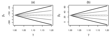
Figure 1: Bounds for $\beta_{1}$ and $\beta_{2}$ for the birthweight dataset, assuming the MSM $g(a;\beta)=\beta_{0}+\beta_{1}a+\beta_{2}a^{2}$. The dotted horizontal lines are at $\widehat{\beta}_{1}$ and $\widehat{\beta}_{2}$. The black bounds are from $F_{1}$ over ${\cal V}_{\rm large}$ for the propensity model, found using the homotopy algorithm (Section 4.4). The local approximation to $F_{1}$ (Section 4.6) matched the black bounds closely (not shown), similar to the appendix examples. The quadratic term parameter loses significance at $\gamma\approx 1.11$ and the linear term at $\gamma\approx 1.25$. The dark and light grey bounds use the subset sensitivity model (Sections 3.3 and A.2), with $\epsilon=.5$ and $.1$, respectively. Bounds are all the narrower when $\epsilon$ is smaller, as expected.

We re-analyzed a dataset of births in Pennsylvania between 1989 and 1991, which has been used to investigate the causal effects of mothers’ smoking behavior on infants birthweight. Previous analyses (Almond et al., 2005; Cattaneo, 2010), assuming no unmeasured confounders, found a negative effect of smoking on the infant’s weight. Recently, Scharfstein et al. (2021) conducted a sensitivity analysis to the assumption of no unmeasured confounding by dichotomizing the treatment into smoking vs non-smoking. In line with previous work, they found a negative effect of smoking on the child’s weight, but also identified plausible values of their sensitivity parameters consistent with a null effect. They concluded that, while likely negative, the true effect of smoking on weight might be smaller than that estimated under no unmeasured confounding. We complement and expand on their analysis by considering sensitivity models that can accommodate MSMs; we reach similar conclusions, although we find the estimated effect to be less sensitive to the unmeasured confounding parametrized by our sensitivity models.

The dataset consists of a random subsample of $5,000$ observations from the original dataset that is available online. The outcome is birthweight and the treatment is an ordered categorical variable taking six values corresponding to ranges $\{0,1\text{-}5,6\text{-}10,11\text{-}15,16\text{-}20,21+\}$ of cigarettes smoked per day. There are 53 pre-treatment covariates including mother’s and father’s education, race, and age; mother’s marital status and foreign born status; indicators for trimester of first prenatal care visit and mother’s alcohol use.

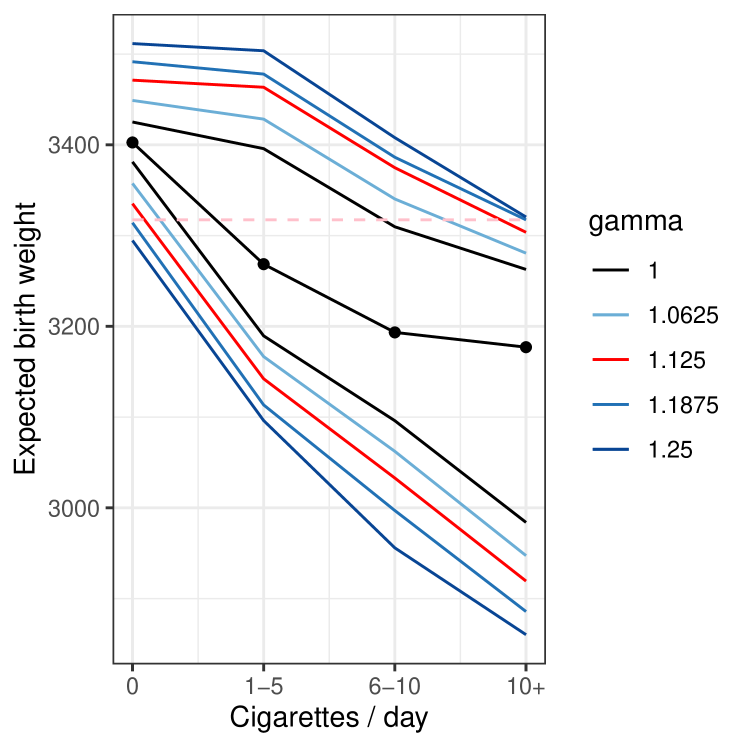
(a) Estimated bands for the linear MSM $g(a;\beta)=\beta_{0}+\beta_{1}a+\beta_{2}a^{2}$.

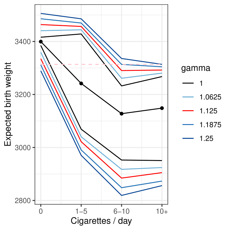
(b) Estimated bands for the saturated MSM $g(a;\beta)=\beta_{0}+\sum_{j=1}^{4}\beta_{j}\mathbbm{1}\{a_{j}\in j^{\text{th}}\text{bin}\}$.

Figure 2: Pointwise 95%-confidence bands on the bounds for $\mbox{$\mathbb{E}$}\{Y(a)\}=g(a;\beta)$ under the propensity sensitivity model, where $a\in\{0,1$–$5,6$–$10,10+\}$ cigarettes per day. The lines with dots are $g(a;\widehat{\beta})$.

Figure 1 shows bounds on $\beta_{1}$ and $\beta_{2}$ for the quadratic MSM given by $g(a;\beta)=\beta_{0}+\beta_{1}a+\beta_{2}a^{2}$ under propensity sensitivity, based on $F_{1}$ over ${\cal V}_{\rm large}$ (with only six treatment values, we cannot fit a more complex parametric model). We estimated the propensity $\pi(a|x)$ via a log-linear neural net using the nnet package for the R software, as in Cattaneo (2010). The quadratic term parameter loses significance at $\gamma\approx 1.11$ and the linear term at $\gamma=1.25$. Figure 1 also shows bounds on $\beta_{1}$ and $\beta_{2}$ under the subset sensitivity model with $\epsilon=.5$ and $.1$. As expected, there is much less sensitivity for small $\epsilon$.

Recall from (5) that $\gamma$ measures the change in the propensity score when $U$ is dropped. To determine if $\gamma=1.25$ constitutes substantial confounding, we followed the ideas in Cinelli and Hazlett (2020) by assessing changes to the propensity score when observed confounders are dropped. Most authors drop one covariate at a time but with 53 covariates, we found that this caused almost no changes to the propensity score. Instead, we (i) dropped half of the covariates, and (ii) computed, for each data point, the ratio of propensity scores using all the covariates and the randomly chosen subset, and repeated (i, ii) 100 times. Each repeat yielded a distribution of propensity score ratios and we used the average of their 80th percentiles as a measure of substantial confounding. This value is $\gamma=1.20$, so we conclude that the causal effect of smoking on infant birthweight remains significant even under substantial confounding. The next analysis confirms this conclusion.

Next, Figure 2 shows $95\%$ point-wise confidence bands for the bounds on $g(a;\beta)$ under propensity sensitivity based on $\mathcal{V}_{\text{small}}$, assuming that the bounds are modeled as $g(a;\beta_{\ell})$ and $g(a;\beta_{u})$; see Proposition 3. Note that Figure 1 showed the bounds on $\beta_{1}$ and $\beta_{2}$ rather than confidence bands on these bounds, because confidence bands are difficult to obtain; see Sections 4.4 and 4.5. Figure 2(a) shows results for the quadratic MSM $g(a;\beta)=\beta_{0}+\beta_{1}a+\beta_{2}a^{2}$, and as a safeguard against MSM mis-specification, Figure 2(b) shows the saturated parametric MSM fit. The black bands corresponding to $\gamma=1$ assume no-unmeasured-confounding (so they are confidence bands for $g(a;\widehat{\beta})$) and increasing values of $\gamma$ correspond to increasing amount of unmeasured confounding. We estimated the nuisance functions nonparametrically: the outcome model $\mu(x,a)$ and conditional quantiles $q_{j}(Y|a,x)$ were fitted assuming generalized additive models, with mother’s and father’s ages, education and birth order entering the model linearly, and number of prenatal care visits and months since last birth entering the model as smooth terms – we used the mgcv and qgam packages in R, respectively; the propensity $\pi(a|x)$ was estimated via a log-linear neural net, as above. We constructed the $95\%$ point-wise confidence bands relying on Proposition 3 and the Hulc method by Kuchibhotla et al. (2021). For the Hulc, the sample needs to be split into six subsamples, but because of small sample sizes in some categories, we collapsed all regimes of 10+ cigarettes into one category, thereby reducing the number of treatment regimes to four. Consistent with Figure 1 and previous analyses (Almond et al., 2005; Cattaneo, 2010), we found a statistically significant negative relationship between smoking and birthweight under no-unmeasured-confounding. The relation ceases to be significant for $\gamma=1.1875$ when the quadratic model is used and $\gamma=1.25$ when the saturated model is used.

7.2 Effect of Mobility on Covid-19 Deaths

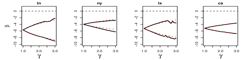
Figure 3: Bounds on $\beta$ in MSM (18) for the Covid data in four US states. The black bounds are from $F_{1}$ over ${\cal V}_{\rm large}$ with increasing amount of unobserved confounding, under the propensity confounding model. The occasional lack of smoothness is due to estimating the quantile $q$ from small samples ($n=40$) in the homotophy algorithm (Section B.1). The dotted red bounds are the local approximations to $F_{1}$ (Section 4.6). The MSM coefficients remain significant under substantial unobserved confounding for the four states: mobility has a significant effect on Covid deaths.

Figure 4: Bounds for counterfactual deaths $\psi(a_{T})=\mbox{$\mathbb{E}$}(Y(a_{T}))$ for the Covid data in four US states using MSM (18) in a hypothetical mobility scenario $a_{T}$ corresponding to shifting the observed mobility pattern two weeks earlier. The bounds are from $F_{1}$ over ${\cal V}_{\rm large}$ under propensity sensitivity, found using the homotopy algorithm. The shades correspond to $\gamma=3$ (white), $\gamma=2$ (light grey) and $\gamma=1$ (no unmeasured confounding, dark grey). The black dots are observed deaths. Our analysis suggests that, even with substantial unobserved confounding, sheltering two weeks earlier would have saved lives, although only by a small number in TN, because the epidemic there started more mildly.

We revisit the analysis in Bonvini et al. (2021) on the causal effects of mobility on deaths due to Covid-19 in the United States. In their paper, a sensitivity analysis to the no unmeasured confounding assumption was conducted under the propensity model without providing details. We provide details here.

The data consist of weekly observations, at the state level, on the number of Covid-19 deaths $Y_{t}$ and a measure of mobility “proportion at home,” $A_{t}$, which is the fraction of mobile devices that did not leave the immediate area of their home. The time period considered in the analysis is February 15 2020 (week 1) to November 15 2020 (week 40). We focus on four states, CA, FL, NY and TN, as representatives of four different evolutions of the pandemic; their observed time series of deaths are plotted as dots in Figure 4. We model each state separately so that differences between states do not act as confounders of the treatment/outcome relationship.

Our MSM is given by

$$g(\overline{a}_{t},\beta,\nu)=\mathbb{E}[L_{t}({\overline{a}_{t}})]=\nu(t)+\beta M_{t}$$ (18)

where $\overline{a}_{t}=(a_{1},\ldots,a_{t})$, $L_{t}(\overline{a}_{t})$ are log-counterfactual deaths, $L_{t}=\log(Y_{t}+1)$, $M_{t}\equiv M(\overline{a}_{t})=\sum_{s=1}^{t-\delta}a_{s}$, and $\delta=4$ weeks is approximately the mean time from infection to death from Covid-19. The nuisance function $\nu(t)$ is assumed to be non-linear to capture changes in death incidence due to time varying variables other than mobility, for example probability of dying, which decreased over time due to better hospital treatment, number of susceptibles to Covid-19, which naturally decreased, and social distancing changes.

Figure 3 shows $\widehat{\beta}$ for the four states, along with lower and upper bounds under propensity sensitivity. The estimates are negative, as would be expected since higher $A_{s}$ means that more people sheltered at home, and they remain negative even under substantial unobserved confounding.

Bonvini et al. (2021) also estimated counterfactual deaths under three hypothetical mobility regimes $\overline{A}_{t}=(A_{1},\ldots,A_{t})$: “start one week earlier” and “start two weeks earlier”, which shifts the observed mobility profiles back by one or two weeks with aim to assess Covid-19 infections if we had started sheltering in place one and two weeks earlier; and “stay vigilant”, which halves the slope of the rapid decrease in stay at home mobility after the initial peak in week 9, when a large proportion of the population hunkered down after witnessing the situation in New York city. To save space, Figure 4 shows only the estimated counterfactual deaths and bounds for the “start two weeks earlier” scenario. Bounds were computed on $g(\overline{a}_{t};\beta)$ for each $t$ using the homotopy algorithm on $F_{1}$ over ${\cal V}_{\rm large}$, under propensity sensitivity (Section 4.4).

Bounds for $\beta$ and $g(\overline{a}_{t};\beta)$ under the outcome sensitivity model requires an outcome model, which we do not pursue here.

8 Conclusion

We have derived several sensitivity analysis methods for marginal structural models. Doing so may require additional modeling, for example, using quantile regression. We also saw that approximate, conservative bounds are possible without quantile regression.

We have focused on the traditional interventions corresponding to setting the treatment to a particular value. In a future paper, we address sensitivity analysis under stochastic interventions. Here we find that these interventions can lead to inference that is less sensitive to unmeasured confounding than traditional interventions.

One issue that always arises in sensitivity analysis is how to systematically choose ranges of values for the sensitivity parameters (e.g., $\gamma$, $\delta$, $\epsilon$, in our case). In the smoking example, we dropped large sets of observed confounders to provide a benchmark, but for the most part this is an open problem.

9 Acknowledgements

We thank Prof. Nicole Pashley for helpful discussions regarding the interpretation of the causal effect of mobility on deaths due to Covid-19. In particular, unmeasured confounding is not the only issue that needs to be addressed when interpreting our results. A potential complication is that there could be multiple versions of mobility, e.g. a person may move to go to work versus a bar. These different versions of mobility may affect the probability of dying due to Covid-19 differently, complicating the interpretation of the overall effect of reduced mobility on deaths. Conducting a sensitivity analysis to gauge the impact of multiple versions of the same treatment is an important avenue for future work.

Appendix A Appendix

A.1 Synthetic Examples

As a proof of concept, we consider a simple simulated example. We take $n=100$, $A_{1},\ldots,A_{n}\sim N(0,1)$ and $Y_{i}=\beta A_{i}+\epsilon_{i}$ where $\epsilon_{i}\sim N(0,1)$. Figure 6a shows the propensity sensitivity bounds for $\beta=3$ based on the homotopy algorithm and using the local approximation; the local method is an excellent approximation. We also conducted a few simulations using very small sample sizes where the exact solution can be computed by brute force. We found that the homotopy method was indistinguishable from the exact bound. Figure 6b shows the bounds using the outcome sensitivity approach.

Now we look at the effect of bounding over ${\cal V}_{\rm large}$ using $F_{1}$ and $F_{2}$. The example in Figure 6 shows that the propensity sensitivity bounds from $F_{2}$ (green) are wider than bounds from $F_{1}$ (black). In this case we used $n=1000$,1 $X\sim N(0,1)$, $A=X+N(0,1)$, $Y=\beta A+2X+N(0,1)$, with $\beta=3$. Conversely, the example in Figure 6b shows that the propensity sensitivity bounds from $F_{2}$ (green) are narrower than bounds from $F_{1}$ (black). Here we used $n=1000$ with: $U\sim{\rm Unif}(.5,1)$, $A=3-U$, $Y=5U$ and $Y=2.5U+.25N(0,1)$. The red dotted lines are the local approximations to the $F_{1}$ bounds, which are very good in these two examples as well. Our experience is that usually $F_{1}$ gives tighter bounds.

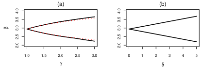
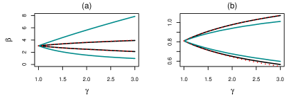
Figure 5: (a) Propensity sensitivity model bounds and (b) Outcome sensitivity model bounds for $\beta$ in the MSM $g(a;\beta)=\beta a$ with $\beta=3$, for a simulated example. In (a), the black bounds in are from $F_{1}$ over ${\cal V}_{\rm large}$, obtained by the homotopy algorithm (Section 4.4), and their local approximations (Section 4.6) are in dotted red.

Figure 6: Propensity sensitivity model bounds from $F_{1}$ (black) and $F_{2}$ (green) over ${\cal V}_{\rm large}$, in simulated examples. Bounds from $F_{2}$ are computationally easier to obtain than bounds from $F_{1}$. The local approximations to $F_{1}$, which are also simple to obtain, are in dotted red. (a) In this example, bounds from $F_{2}$ are wider than bounds from $F_{1}$, so we use the latter. (b) In this other example, the reverse is true. We do not know in advance which bounds to use.

A.2 Subset Confounding

Recall that, under this model, an unknown proportion of the population is subject to unobserved confounding. Suppose $S$ is such that $Y(a)\perp\!\!\!\perp A|X,S=1$ but $Y(a)\perp\!\!\!\perp A|X,U,S=0$ where $U$ is not observed. That is, $S=0$ represents the subset with unmeasured confounding and $S=1$ represents the subset with no unmeasured confounding. This is a sensitivity model proposed by Bonvini and Kennedy [2021] in the case of binary treatments. Here, we extend this framework to multivalued treatments and MSMs under the propensity sensitivity model and the outcome sensitivity model. To start, we define the propensity model in this case to be

$$\gamma^{-1}\leq\frac{\pi(a|x,u,S=0)}{\pi(a|x,S=0)}\leq\gamma\quad\text{ for all }a,x,u.$$

Let

$$v_{0}(Z)=\mbox{$\mathbb{E}$}\left\{\frac{\pi(A|X,S=0)}{\pi(A|X,S=0,U)}\ \Big{|}\ Y,A,X,S=0\right\}$$

and notice that $\mbox{$\mathbb{E}$}\{v_{0}(Z)|A,X,S=0\}=1$ and $v_{0}(Z)\in[\gamma^{-1},\gamma]$. Essentially, we can repeat the same calculations as in the non-contaminated model, this time simply applied to the $S=0$ group.

The same argument used in proving Lemma 2 yields that

$$\mbox{$\mathbb{E}$}\{Y\gamma^{\operatorname{sgn}\{q_{\ell}(Y|a,x,S=0)-Y\}}|A=a,X=x,S=0\}$$

$$\leq\mbox{$\mathbb{E}$}\{Yv_{0}(Z)|A=a,X=x,S=0\}\leq$$

$$\mbox{$\mathbb{E}$}\{Y\gamma^{\operatorname{sgn}\{Y-q_{u}(Y|a,x,S=0)\}}|A=a,X=x,S=0\}$$

where $q_{\ell}(Y|a,x,S=0)$ and $q_{u}(Y|a,x,S=0)$ are the $\tau_{\ell}=1/(\gamma+1)$ and $\tau_{u}=\gamma/(1+\gamma)$ quantiles of the distribution of $Y|(A,X,S=0)$. As in Bonvini and Kennedy [2021], we make the simplifying assumption that $S\perp\!\!\!\perp Y|A,X$. This way,

$$m_{\ell}(a,x)\equiv\mbox{$\mathbb{E}$}\{Y\gamma^{\operatorname{sgn}\{q_{\ell}(Y|a,x)-Y\}}|A=a,X=x\}$$

$$\leq\mbox{$\mathbb{E}$}\{Yv_{0}(Z)|A=a,X=x,S=0\}\leq$$

$$\mbox{$\mathbb{E}$}\{Y\gamma^{\operatorname{sgn}\{Y-q_{u}(Y|a,x)\}}|A=a,X=x\}\equiv m_{u}(a,x)$$

where now the quantile are those of the distribution of $Y|(A,X)$. Notice that these are the usual bounds in the non-contaminated model.

We can then compute the bounds on $\mbox{$\mathbb{E}$}\{Y(a)|X\}$. First notice that,

$$\mbox{$\mathbb{E}$}\{Y(a)S|X\} =\mbox{$\mathbb{E}$}(Y|A=a,X,S=1)\mathbb{P}(S=1|X) (Y(a)\perp\!\!\!\perp A|X,S=1)$$

$$=\mu(a,X)\mathbb{P}(S=1|X). (Y\perp\!\!\!\perp S|A,X)$$

This means that $\mbox{$\mathbb{E}$}\{Y(a)S\}=\mbox{$\mathbb{E}$}\{S\mu(a,X)\}$. Next notice that

$$\mbox{$\mathbb{E}$}\{Y(a)(1-S)|X\} =\mbox{$\mathbb{E}$}\{Y(a)|X,S=0\}\mathbb{P}(S=0|X)$$

$$=\mbox{$\mathbb{E}$}\{Y\alpha(a,X,U,S=0)|A=a,X,S=0\}\mathbb{P}(S=0|X)$$

$$=\mbox{$\mathbb{E}$}\{Yv_{0}(Z)|A=a,X,S=0\}\mathbb{P}(S=0|X).$$

Therefore,

$$\mbox{$\mathbb{E}$}\{Y(a)|X\}=\mu(a,X)\mathbb{P}(S=1|X)+\mbox{$\mathbb{E}$}\{Yv_{0}(Z)|A=a,X,S=0\}\mathbb{P}(S=0|X)$$

so that

$$\mbox{$\mathbb{E}$}\{Y(a)\}=\mbox{$\mathbb{E}$}\left\{\mu(a,X)\right\}+\mbox{$\mathbb{E}$}\left[(1-S)\left\{\mbox{$\mathbb{E}$}\{Yv_{0}(Z)|A=a,X,S=0\}-\mu(a,X)\right\}\right]$$

which implies, for $r_{j}(a,X)=m_{j}(a,X)-\mu(a,X)$ and $j\in\{l,u\}$:

$$\mbox{$\mathbb{E}$}\{\mu(a,X)+(1-S)r_{\ell}(a,X)\}\leq\mbox{$\mathbb{E}$}\{Y(a)\}\leq\mbox{$\mathbb{E}$}\{\mu(a,X)+(1-S)r_{u}(a,X)\}.$$

Let $t_{\epsilon,l}(a)$ the $\epsilon$-quantile of $r_{\ell}(a,X)$ and $t_{\epsilon,u}$ be the $(1-\epsilon)$-quantile of $r_{u}(a,X)$. Further, let $\lambda_{\ell}(a,x)=\mathbbm{1}\{r_{u}(a,x)\leq t_{\epsilon,l}(a)\}$ and $\lambda_{u}(a,x)=\mathbbm{1}\{r_{u}(a,x)>t_{\epsilon,u}(a)\}$. Under the assumption that $\mathbb{P}(S=0)=\epsilon$, we bound $\mbox{$\mathbb{E}$}\{Y(a)\}$ by further optimizing over $S$ as

$$\mbox{$\mathbb{E}$}\{Y(a)\}\geq\mbox{$\mathbb{E}$}\{\mu(a,X)\}+\mbox{$\mathbb{E}$}[\lambda_{\ell}(a,X)r_{\ell}(a,X)]\equiv\theta_{\ell}(a)$$

$$\mbox{$\mathbb{E}$}\{Y(a)\}\leq\mbox{$\mathbb{E}$}\{\mu(a,X)\}+\mbox{$\mathbb{E}$}[\lambda_{u}(a,X)r_{u}(a,X)]\equiv\theta_{u}(a).$$

As discussed in Section 4.2, one option to estimate the bounds is to assume that they follow some parametric models $g(a;\beta_{\ell})$ and $g(a;\beta_{u})$. Define

$$f_{\mu}(Z_{1},Z_{2})=W(A_{1},X_{1})\{Y_{1}-\mu(A_{1},X_{1})\}+\mu(A_{1},X_{2})$$

$$f_{\Delta,j}(Z_{1})=W(A_{1},X_{1})\left[\left\{s_{j}(Z;q_{j})-\kappa(A_{1},X_{1};q_{j})\right\}-Y_{1}+\mu(A_{1},X_{1})\right]$$

$$f_{r,j}(Z_{1},Z_{2})=\kappa(A_{1},X_{2};q_{j})-\mu(A_{1},X_{2})$$

$$f_{j}(Z_{1},Z_{2})=f_{\mu}(Z_{1},Z_{2})+\lambda_{j}(A_{1},X_{1})f_{\Delta,j}(Z_{1})+\lambda_{j}(A_{1},X_{2})f_{r,j}(Z_{1},Z_{2}).$$

Then, if it is assumed that $\theta_{j}(a)=g(a;\beta_{j})$, the following moment condition holds

$$\mathbb{U}\left[h(A_{1})\left\{f_{j}(Z_{1},Z_{2})-g(A_{1};\beta_{j})\right\}\right]=0.$$

In this respect, we define $\widehat{\beta}_{j}$ to solve $\mathbb{U}_{n}\left[h(A_{1})\left\{\widehat{f}_{j}(Z_{1},Z_{2})-g(A_{1};\widehat{\beta}_{j})\right\}\right]=0$. We estimate the nuisance functions on a separate sample $D^{n}$ independent from the sample $Z^{n}$ used to evaluate the $U$-statistic. However, in the proof of the proposition below, we require that $\widehat{t}_{\epsilon,j}(a)$ satisfies

$$\frac{1}{n}\sum_{i\in Z^{n}}\mathbbm{1}\{\widehat{r}_{j}(a,X_{i})>\widehat{t}_{\epsilon,j}(a)\}=\epsilon+o_{\mathbb{P}}(n^{-1/2})\text{ for all }a\in\mathcal{A}\text{ and }j=\{l,u\}.$$

In other words, we estimate all nuisance functions on a separate, training sample except for $a\mapsto t_{1-\epsilon}(a)$, which is estimated on the same sample used to estimate the moment condition. This helps with controlling the bias due to the presence of the indicator at the expense of an additional requirement on the complexity of the class where $a\mapsto\widehat{t}_{\epsilon,j}(a)$ belongs to. We have the following proposition.

Proposition 11

Suppose

1. The function class $\mathcal{G}_{l}=\left\{a\mapsto h_{l}(a)g(a;\beta)\right\}$ is Donsker for every $l=\{1,\ldots,k\}$ with integrable envelop and $g(a;\beta)$ is a continuous function of $\beta$;

2. The map $\beta\mapsto\mathbb{U}\{h(A_{1})f_{j}(Z_{1},Z_{2})-g(A_{1};\beta)\}$ is differentiable at all $\beta$ with continuosly invertible matrices $\dot{\Psi}_{\beta_{0}}$ and $\dot{\Psi}_{\widehat{\beta}}$, where $\dot{\Psi}_{\beta}=-\mbox{$\mathbb{E}$}\{h(A)\nabla^{T}g(A;\beta)\}$;

3. The function class $\mathcal{T}$ where $a\mapsto\widehat{t}_{\epsilon,j}(a)$ and $a\mapsto t_{\epsilon,j}(a)$ belong to is VC-subgraph;

4. For any $a\in\mathcal{A}$ and $x\in\mathcal{X}$, $r_{j}(a,X)-t_{\epsilon,j}(a)$, $r_{j}(A,x)-t_{\epsilon,j}(A)$ and $r_{j}(A,X)-t_{\epsilon,j}(A)$ have bounded densities;

5. The following holds

   $$\lVert\widehat{q}_{u}-q_{u}\rVert=o_{\mathbb{P}}(n^{-1/4}),\ \left\|r_{j}-\widehat{r}_{j}\right\|_{\infty}+\left\|t_{\epsilon,j}-\widehat{t}_{\epsilon,j}\right\|_{\infty}=o_{\mathbb{P}}(n^{-1/4})$$

   $$\left(\left\|r_{j}-\widehat{r}_{j}\right\|_{\infty}+\left\|t_{\epsilon,j}-\widehat{t}_{\epsilon,j}\right\|_{\infty}+\lVert\widehat{w}-w\rVert\right)\left(\lVert\widehat{\mu}-\mu\rVert+\lVert\kappa_{j}-\widehat{\kappa}_{j}\rVert\right)=o_{\mathbb{P}}(n^{-1/2}).$$

Then,

$$\sqrt{n}(\widehat{\beta}_{j}-\beta_{j})\rightsquigarrow N(0,4\Sigma)$$

where $\Sigma=\text{var}\left[\dot{\Psi}^{-1}_{\beta_{j}}\int S_{2}h(A_{1})\left\{f_{j}(Z_{1},z_{2})-t_{\epsilon,j}(A_{1})\lambda_{j}(A_{1},x_{2})-g(A_{1};\beta_{j})\right\}d\mathbb{P}(z_{2})\right].$

To get bounds on some coordinate of $\beta$, say $\beta_{1}$, one may proceed by homotopy as in the non-contaminated model. In the linear MSM case, i.e. $g(a;\beta)=b(a)^{T}\beta$, bounds on $\beta_{1}$ that enforce the restriction $\mbox{$\mathbb{E}$}\{v_{0}(Z)|A,X,S=0\}=1$ would be

$$l_{\gamma}=\int\min\left\{e^{T}M^{-1}b(a)\theta_{u}(a),e^{T}M^{-1}b(a)\theta_{\ell}(a)\right\}d\mathbb{P}(a)$$

$$u_{\gamma}=\int\max\left\{e^{T}M^{-1}b(a)\theta_{u}(a),e^{T}M^{-1}b(a)\theta_{\ell}(a)\right\}d\mathbb{P}(a)$$

where $M=\mbox{$\mathbb{E}$}\{b(A)b(A)^{T}\}$ and we set $h(A)=b(A)$. A similar statement to Proposition 4 can be derived using the influence function established in proving Proposition 11.

Remark: If we make the stronger assumption that $S$ is independent of $(X,A,Y)$ then $p_{0}(x,a,y)=p_{1}(x,a,y)$. In this case it is easy to see that $\mbox{$\mathbb{E}$}[h(A)(Y-g(A,\beta))w(A,X)((1-\epsilon)+\epsilon v(Z))]=0$. All the previous methods can then be used with $v$ replaced with $(1-\epsilon)+\epsilon v(Z)$.

Now we use the outcome sensitivity model on the confounded subpopulation. We will assume that $S\perp\!\!\!\perp Z$. The distribution is

$$(1-\epsilon)p(u,x,a)p(y|x,a)+\epsilon p(u,x,a)p(y|u,x,a).$$

The moment condition is

$$0 =\int b(a)(y-b^{T}(a)\beta)w(u,x,a)dP(u,x,a)$$

$$=(1-\epsilon)\int b(a)(y-b^{T}(a)\beta)w(u,x,a)p(u,x,a)p(y|x,a)+\epsilon\int b(a)(y-b^{T}(a)\beta)w(u,x,a)p(u,x,a)p(y|u,x,a)$$

$$=(1-\epsilon)\int b(a)(y-b^{T}(a)\beta)w(x,a)p(x,a)p(y|x,a)+\epsilon\int b(a)(y-b^{T}(a)\beta)w(u,x,a)p(u,x,a)p(y|u,x,a)$$

$$=(1-\epsilon)\int b(a)(y-b^{T}(a)\beta)w(x,a)p(x,a)p(y|x,a)+\epsilon\int b(a)(y-\mu(x,a))w(u,x,a)p(u,x,a)p(y|u,x,a)$$

$$\hskip 28.45274pt+\epsilon\int b(a)(\mu(x,a)-b^{T}(a)\beta)w(u,x,a)p(u,x,a)p(y|u,x,a)$$

$$=(1-\epsilon)\int b(a)(y-b^{T}(a)\beta)w(x,a)p(x,a)p(y|x,a)+\epsilon\underbrace{\int b(a)(\mu(u,x,a)-\mu(x,a))w(u,x,a)p(u,x,a)}_{\Xi}$$

$$\hskip 28.45274pt+\epsilon\int b(a)(\mu(x,a)-b^{T}(a)\beta)w(x,a)p(x,a)$$

$$=(1-\epsilon)\int b(a)(y-b^{T}(a)\beta)w(x,a)p(x,a)p(y|x,a)+\epsilon\int b(a)(\mu(x,a)-b^{T}(a)\beta)w(x,a)p(x,a)p(y|x,a)+\epsilon\Xi$$

$$=\mbox{$\mathbb{E}$}\Biggl{[}b(A)\Bigl{(}(1-\epsilon)Y+\epsilon\mu(X,A)\Bigr{)}w(X,A)\Biggr{]}-\underbrace{\Biggl{(}\mbox{$\mathbb{E}$}[b(A)b^{T}(A)w(X,A)]\Biggr{)}}_{\Omega}\beta+\epsilon\Xi,$$

where $\Xi=\int b(a)(\mu(u,x,a)-\mu(x,a))w(u,x,a)p(u,x,a)$ and $\Omega=\mbox{$\mathbb{E}$}[b(A)b^{T}(A)w(X,A)].$ Therefore

$$\beta=\Omega^{-1}\mbox{$\mathbb{E}$}\Biggl{[}b(A)\Bigl{(}(1-\epsilon)Y+\epsilon\mu(X,A)\Bigr{)}w(X,A)\Biggr{]}+\epsilon\Omega^{-1}\Xi$$

and $\beta_{1}=e^{T}\beta$, where $e=(1,0,\ldots,0)$. Let $r$ be the first row of $\Omega^{-1}$ and let $f(a)=\sum_{j}r_{j}b_{j}(a)$. Then

$$e^{T}\Omega^{-1}\Xi =r^{T}\Xi=\int(\sum_{j}r_{j}b_{j}(a))(\mu(u,x,a)-\mu(x,a))w(u,x,a)p(u,x,a)$$

$$\leq\delta\int f(a)I(f(a)>0)\pi(a)-\delta\int f(a)I(f(a)<0)\pi(a)$$

$$=\delta\int f(a)(2I(f(a)>0)-1)\pi(a).$$

Similarly,

$$e^{T}\Omega^{-1}\Xi\geq\delta\int f(a)I(f(a)<0)\pi(a)-\delta\int f(a)I(f(a)>0)\pi(a)\\ -\delta\int f(a)(2I(f(a)>0)-1)\pi(a).$$

Therefore,

$$\beta_{1}^{*}-\delta\int f(a)(2I(f(a)>0)-1)\pi(a)\leq\beta_{1}\leq\beta_{1}^{*}+\delta\int f(a)(2I(f(a)>0)-1)\pi(a)$$

where

$$\beta_{1}^{*}=\mbox{$\mathbb{E}$}\Biggl{[}b(A)\Bigl{(}(1-\epsilon)Y+\epsilon\mu(X,A)\Bigr{)}w(X,A)\Biggr{]}.$$

A.3 Bounds for $\beta$ under the outcome sensitivity confounding model when the MSM is not linear

Say the MSM is not linear. Since $g(a;\beta)=\mbox{$\mathbb{E}$}\{Y(a)\}=\int\int yp(y|u,x,a)dP(x,u)$, we have

$$0 =\int\int\int h(a)(y-g(a;\beta))p(y|u,x,a)\pi(a)dydP(u,x)$$

$$=\int\int h(a)(\mu(u,x,a)-g(a;\beta))\pi(a)dP(u,x)$$

$$=\int\int h(a)(\mu(u,x,a)-\mu(x,a))\pi(a)dP(u,x)+\int\int h(a)(\mu(x,a)-g(a;\beta))\pi(a)dP(u,x)$$

$$=\int\int h(a)(\mu(u,x,a)-\mu(x,a))\pi(a)dP(u,x)+\int\int h(a)(\mu(x,a)-g(a;\beta))\pi(a)dP(x)$$

$$=\int\int h(a)(\mu(u,x,a)-\mu(x,a))\pi(a)dP(u,x)+\int\int\frac{h(a)(\mu(x,a)-g(a;\beta))\pi(a)}{\pi(a|x)}\pi(a|x)dP(x)$$

$$=\int h(a)\xi(a)\pi(a)da+\mbox{$\mathbb{E}$}[h(A)(\mu(X,A)-g(A;\beta))w(A,X)].$$

Let $C=\{\mbox{$\mathbb{E}$}[h_{1}(A)\xi(A)],\ldots,\mbox{$\mathbb{E}$}[h_{k}(A)\xi(A)]:\ -\delta\leq\xi(a)\leq\delta\}$. For each vector $t\in C$, let $\beta(t)$ solve $\mbox{$\mathbb{E}$}[h(A)(\mu(X,A)-g(A;\beta))w(A,X)]=t$. Then

$$\inf_{t\in C}e^{T}\beta(t)\leq\beta_{j}\leq\sup_{t\in C}e^{T}\beta(t).$$

These bounds can be found numerically by solving for $\beta(t)$ over a grid on $C$.

Appendix B Algorithms

B.1 Homotopy Algorithm

Input: grid $\{\gamma_{1},\ldots,\gamma_{N}\}$ where $\gamma_{1}=1$ and $\gamma_{1}<\cdots<\gamma_{N}$.

1. Let $\widehat{\beta}$ be the solution of $\sum_{i}h(A_{i})(Y_{i}-g(A_{i};\widehat{\beta}))\widehat{W}_{i}=0$. Let $u_{1}=\ell_{1}=e^{T}\widehat{\beta}$.

2. For $j=2,\ldots,N$:

   1. Let $d_{j,i}\equiv d_{\gamma_{j-1},i}$ from (14) evaluated at $v=v_{\gamma_{j}-1}$.

   2. Set $V_{i}=\gamma_{j}^{-1}I(d_{j,i}\leq q)+\gamma_{j}I(d_{j,i}>q)$ where $q$ is the $\gamma_{j}/(1+\gamma_{j})$ quantile of $d_{j,1},\ldots,d_{j,n}$. Let $\widehat{\beta}$ be the solution of $\sum_{i}h(A_{i})(Y_{i}-g(A_{i};\widehat{\beta}))\widehat{W}_{i}V_{i}=0$. Set $u_{j}=e^{T}\widehat{\beta}$.

   3. Set $V_{i}=\gamma_{j}I(d_{j,i}\leq q)+\gamma_{j}^{-1}I(d_{j,i}>q)$ where $q$ is the $1/(1+\gamma_{j})$ quantile of $d_{j,1},\ldots,d_{j,n}$. Let $\widehat{\beta}$ be the solution of $\sum_{i}h(A_{i})(Y_{i}-g(A_{i};\widehat{\beta}))\widehat{W}_{i}V_{i}=0$. Set $\ell_{j}=e^{T}\widehat{\beta}$.

3. Return $(\ell_{1},u_{1}),\ldots,(\ell_{N},u_{N})$.

B.2 Bounds on $\beta$ by Coordinate Ascent

Another approach we consider is coordinate ascent where we maximize (or minimize) $\widehat{\beta}_{1}(v)$ over each coordinate $v_{i}$ in turn. It turns out that this is quite easy since $\widehat{\beta}_{1}(v)$ is strictly monotonic in each $v_{i}$ for many models so we need only compare the estimate at the two values $v_{i}=\gamma$ and $v_{i}=1/\gamma$. Furthermore, in the linear case, getting the estimate after changing one coordinate $v_{i}$ can be done quickly using a Sherman-Morrison rank one update.

The coordinate ascent approach will lead to a local optimum but it will depend on the ordering of the data so we repeat the algorithm using several random orderings. The homotopy method instead uses the last solution as a starting point for the new solution. This makes the homotopy method faster but, in principle, the coordinate ascent approach could explore a wider set of possible solutions. For simplicity, the only restriction we enforce is $1/\gamma\leq v_{i}\leq\gamma$. In practice, we find that the solutions are very similar.

Lemma 12

Suppose that the function $\widehat{\beta}(v)$ is strictly monotonic in each coordinate $v_{i}$. The maximizer and minimizer occur at corners of the cube $[1/\gamma,\gamma]^{n}$. We have that

$$\frac{\partial\widehat{\beta}_{1}(v)}{\partial v_{j}}=\frac{1}{W_{i}}e^{T}\Bigl{\{}(X^{T}\mathbb{W}X)^{-1}[S_{i}-(R_{i}R_{i}^{T})\widehat{\beta}]\Bigr{\}}$$

where $W_{i}=1/\pi(A_{i}|X_{i})$, $\mathbb{W}$ is diagonal with $\mathbb{W}_{ii}=W_{i}$, $R_{i}=(X_{i1},\ldots,X_{id})^{T}$ and $S_{i}=R_{i}Y_{i}$. Also,

$$H_{ij}\equiv\frac{\partial^{2}\widehat{\beta}_{1}}{\partial v_{i}\partial v_{j}}=-e^{T}(X^{T}\mathbb{W}X)^{-1}\Biggl{\{}(R_{i}R_{i}^{T})\frac{\partial\widehat{\beta}}{\partial v_{i}}+(R_{j}R_{j}^{T})\frac{\partial\widehat{\beta}}{\partial v_{j}}\Biggr{\}}.$$

The proof is straightforward and is omitted.

Coordinate Ascent

1. Input: Data $(B,A,Y)$, where $B$ is the $n\times k$ matrix with elements $B_{ij}=b_{j}(A_{i})$, weights $W_{i}=1/\pi(A_{i}|X_{i})$ and grid $\{\gamma_{1},\ldots,\gamma_{N}\}$ with $\gamma_{1}=1$.

2. Let $\widehat{\beta}=(B^{T}\mathbb{W}B)^{-1}B^{T}\mathbb{W}Y$ where $\mathbb{W}$ is diagonal with $\mathbb{W}_{ii}=W_{i}$. Set $\overline{\beta}_{1}(1)=\underline{\beta}_{1}(1)=\widehat{\beta}_{1}$.

3. Now move $v_{i}=1$ to $v_{i}=\gamma_{2}$ or $v_{i}=1/\gamma_{2}$, whichever makes $\widehat{\beta}_{1}$ larger:

   1. Let $G=(B^{T}\mathbb{W}B)$. For each $i$ let

      $$u_{i} =e^{T}\Biggl{(}G^{-1}_{i}-\frac{\Delta_{i}G^{-1}_{i}r_{i}r_{i}^{T}G^{-1}}{1+\Delta_{i}r_{i}^{T}A^{-1}_{i}r_{i}}\Biggr{)}(B^{T}\mathbb{W}+\Delta_{i}e_{i}e_{i}^{T})Y\ \ \ {\rm flip\ 1\ to\ }\gamma_{2}$$

      $$\ell_{i} =e^{T}\Biggl{(}G^{-1}_{i}-\frac{\delta_{i}G^{-1}r_{i}r_{i}^{T}G^{-1}}{1+\delta_{i}r_{i}^{T}G^{-1}r_{i}}\Biggr{)}(B^{T}\mathbb{W}+\delta_{i}e_{i}e_{i}^{T})Y\ \ \ {\rm flip\ 1\ to\ }1/\gamma_{2}$$

      where $\Delta_{i}=\gamma_{2}-1$ and $\delta_{i}=\frac{1}{\gamma_{2}}-1$.

   2. If $u_{i}\geq\ell_{i}$: set $v_{i}=\gamma_{2}$ and $I_{i}=1$. Else, set $v_{i}=1/\gamma_{2}$ and $I_{i}=0$.

4. For $j=3,\ldots,N$: Try flipping each $v_{i}$ to $1/alpha_{i}$.

   1. Let $v_{i}=\gamma_{j}I_{i}+\gamma_{j}^{-1}(1-I_{i})$.

   2. Let $\mathbb{W}_{ii}=v_{i}$ and $\widehat{\beta}=(B^{T}\mathbb{W}B)^{-1}B^{T}\mathbb{W}Y$.

   3. Let $A=(B^{T}\mathbb{W}B)$,

      $$t_{i} =e^{T}\Biggl{(}A^{-1}_{i}-\frac{\Delta_{i}A^{-1}_{i}r_{i}r_{i}^{T}A^{-1}_{i}}{1+\Delta_{i}r_{i}^{T}A^{-1}_{i}r_{i}}\Biggr{)}(B^{T}\mathbb{W}+\Delta_{i}e_{i}e_{i}^{T})Y.$$

      where $\Delta_{i}=1/v_{i}-v_{i}$. If $t_{i}>\widehat{\beta}_{1}$ let $v_{i}=1/v_{i}$. Let $\mathbb{W}_{ii}=v_{i}$. Let $\widehat{\beta}=(B^{T}\mathbb{W}B)^{-1}B^{T}\mathbb{W}Y$. Let $\overline{\beta}_{1}(\gamma_{j})=\widehat{\beta}_{1}$.

Appendix C Technical proofs

C.1 Proof of Proposition 1

Let $\alpha(u,x,a)=\pi(a|x)/\pi(a|x,u)$. Recall that $v(X,A,Y)=\mbox{$\mathbb{E}$}\{\alpha(U,X,A)\mid X,A,Y\}$ and $w(A,X)=\pi(A)/\pi(A\mid X)$. We have

$$0 =\mbox{$\mathbb{E}$}\left[h(A)w(A,X)\{Y-g(A;\beta)\}\alpha(U,X,A)\right]$$

$$=\mbox{$\mathbb{E}$}\left[h(A)w(A,X)\{Y-g(A;\beta)\}v(X,A,Y)\right]$$

$$=\mbox{$\mathbb{E}$}\left\{h(A)Yv(X,A,Y)-h(A)w(A,X)g(A;\beta)v(X,A,Y)\right\}$$

$$=\mbox{$\mathbb{E}$}\left[h(A)w(A,X)\mbox{$\mathbb{E}$}\{Yv(X,A,Y)|X,A\}-h(A)w(A,X)g(A;\beta)\mbox{$\mathbb{E}$}\{v(X,A,Y)|X,A\}\right]$$

$$=\mbox{$\mathbb{E}$}\left\{h(A)w(A,X)m(X,A)-h(A)w(A,X)g(A;\beta)\right\}$$

$$=\int\int\{h(a)m(x,a)d\mathbb{P}(x)-h(a)g(a;\beta)\}d\mathbb{P}(x)\pi(a)da$$

$$=\mbox{$\mathbb{E}$}\left[h(A)\left\{\int m(A,x)d\mathbb{P}(x)-g(A;\beta)\right\}\right].\ \ \Box$$

C.2 Proof of Lemma 2

We will prove the result for the upper bound. The proof for the lower bound follows analogously. We have $v_{u}(Z)\in[\gamma^{-1},\gamma]$ and we can check that $\mbox{$\mathbb{E}$}\{v_{u}(Z)|A,X\}=1$. Indeed

$$\mbox{$\mathbb{E}$}\{v_{u}(Z)|A,X\} =\gamma\mathbb{P}\left(Y>q_{u}(Y|A,X)|A,X\right)+\frac{1}{\gamma}\mathbb{P}\left(Y\leq q_{u}(Y|A,X)|A,X\right)$$

$$=\gamma\left(1-\frac{\gamma}{1+\gamma}\right)+\frac{1}{\gamma}\cdot\frac{\gamma}{1+\gamma}=1,$$

because $q_{u}(A,X)$ is the $\gamma/(1+\gamma)$-quantile of the conditional distribution of $Y$ given $(A,X)$. Let $v(Z)$ be any function contained in $[\gamma^{-1},\gamma]$ such that $\mbox{$\mathbb{E}$}\{v(Z)|A,X\}=1$. We have

$$\begin{cases}v_{u}(Z)-v(Z)\geq 0&\text{ if }Y>q_{u}(Y|A,X)\\ v_{u}(Z)-v(Z)\leq 0&\text{ if }Y\leq q_{u}(Y|A,X)\end{cases}$$

Therefore, $Y\{v_{u}(Z)-v(Z)\}\geq q_{u}(Y|A,X)\{v_{u}(Z)-v(Z)\}$ so that

$$\mbox{$\mathbb{E}$}\left\{Y\{v_{u}(Z)-v(Z)\}|A,X\right\}\geq q_{u}(Y|A,X)\mbox{$\mathbb{E}$}\{v_{u}(Z)-v(Z)|A,X\}=0$$

as desired.

C.3 Proof of Proposition 3

This proposition follows directly from Lemma C.21, except that we need to show the validity of condition 4. This condition holds under the assumption of Proposition 3 because

$$\mathbb{U}\left[h_{l}(A_{1})\{\widehat{\varphi}_{j}(Z_{1},Z_{2})-\varphi_{j}(Z_{1},Z_{2})\}\right] =\int h_{l}(a)\widehat{w}(a,x)\{\kappa(a,x;\widehat{q}_{j})-\kappa(a,x;q_{j})\}d\mathbb{P}(a,x)$$

$$\hphantom{=}+\int\{w(a,x)-\widehat{w}(a,x)\}\{\widehat{\kappa}(a,x;\widehat{q}_{j})-\kappa(a,x;q_{j})\}d\mathbb{P}(a,x)$$

Therefore, by Cauchy-Schwarz and Lemma C.17:

$$\left|\mathbb{U}\left[h_{l}(A_{1})\{\widehat{\varphi}_{j}(Z_{1},Z_{2})-\varphi_{j}(Z_{1},Z_{2})\}\right]\right|\lesssim\|q_{j}-\widehat{q}_{j}\|^{2}+\|w-\widehat{w}\|\|\widehat{\kappa}_{j}-\kappa_{j}\|.$$

C.4 Proof of Proposition 4

We apply Lemma C.21 to the moment condition

$$\Psi_{n}(\beta)=\mathbb{U}_{n}\left[b(A)\left\{\widehat{f}_{j}^{s}(Z_{1},Z_{2})-b(A_{1})^{T}\beta\right\}\right]=o_{\mathbb{P}}(n^{-1/2})$$

The function class $\mathcal{G}_{l}=\left\{a\mapsto b_{l}(a)b(a)^{T}\beta,\beta\in\mathbb{R}^{k}\right\}$ is Donsker since its a finite dimensional vector space (Lemma 7.15 in Sen [2018]). Thus, it remains to check condition 4. We have

$$\left|\mathbb{U}\left\{\widehat{f}_{j}^{s}(Z_{1},Z_{2})-f_{j}^{s}(Z_{1},Z_{2})\right\}\right| \lesssim\|q_{j}-\widehat{q}_{j}\|^{2}+\|w-\widehat{w}\|\|\kappa_{j}-\widehat{\kappa}_{j}\|+\sup_{a}\left|b_{0}^{T}(\widehat{Q}-Q)h(a)\right|^{2}$$

$$=o_{\mathbb{P}}(n^{-1/2})$$

by assumption and because the last term is $O_{\mathbb{P}}(n^{-1})=o_{\mathbb{P}}(n^{-1/2})$ by Lemma 14.

C.5 Proof of Lemma 5

For $v\in{\cal V}_{\rm small}(\gamma)$ we have $\int\int\int h(a)w(a,x)g(a;b)v(z)dP(z)=\int\int h(a)w(a,x)g(a;b)[\int v(z)p(y|x,a)]\pi(a|x)dP(x)=\int\int h(a)w(a,x)g(a;b)\pi(a|x)dP(x)=\int\int h(a)w(a,x)g(a;b)dP(z)$ since $\mbox{$\mathbb{E}$}[v(Z)|X,A]=1$. Therefore $F_{1}=F_{2}$ and the result follows.

C.6 Proof of Lemma 6

Let $Z=(A,X,Y)$ and $p(z)$ denote its density. From the moment condition, we have that $F_{2}(v)$ satisfies

$$\int h(a)w(a,x)v(z)yd\mathbb{P}(z)=\int h(a)g(a;F_{2}(v))w(a,x)d\mathbb{P}(z)$$

Let $m:\mathcal{F}\mapsto\mathbb{R}$ be a generic functional taking as input a function $f$. The functional derivative of $m$ with respect to $f(z)$, denoted $\frac{\delta}{\delta f}m$, satisfies

$$\frac{d}{d\epsilon}m(f+\epsilon\eta)\Large|_{\epsilon=0}=\int\frac{\delta}{\delta f}m(z)\eta(z)d\mathbb{P}(z)$$

for any function $\eta$. Letting

$$\nabla_{\beta}g(A:\beta)=\begin{bmatrix}\frac{d}{d\beta_{1}}g(A;\beta)\\ \vdots\\ \frac{d}{d\beta_{k}}g(A;\beta)\end{bmatrix},\quad\frac{d}{d\epsilon}F_{2}(v+\epsilon\eta)=\begin{bmatrix}\frac{d}{d\epsilon}F_{2,1}(v+\epsilon\eta)\\ \vdots\\ \frac{d}{d\epsilon}F_{2,k}(v+\epsilon\eta)\end{bmatrix},\quad\text{ and }\quad\frac{\delta}{\delta v}F_{2}(v)=\begin{bmatrix}\frac{\delta}{\delta v}F_{2,1}(v)\\ \vdots\\ \frac{\delta}{\delta v}F_{2,k}(v)\end{bmatrix}$$

and taking the functional derivative with respect to $v(z)$ on both sides of the expression above yields

$$\frac{d}{d\epsilon}\int h(a)w(a,x)\{v(z)+\epsilon\eta(z)\}yp(z)dz\Large|_{\epsilon=0}=\int h(a)w(a,x)y\eta(z)p(z)dz$$

$$\implies\frac{\delta}{\delta v}\int h(a)w(a,x)v(z)yp(z)dz=h(a)w(a,x)y$$

$$\frac{d}{d\epsilon}\int h(a)w(a,x)g(a;\beta(v+\epsilon\eta))p(z)dz\Large|_{\epsilon=0}=\int h(a)w(a,x)\nabla_{\beta}g(a;\beta)^{T}p(z)dz\frac{d}{d\epsilon}\beta(v+\epsilon\eta)\Large|_{\epsilon=0}$$

$$\implies\frac{\delta}{\delta v}\int h(a)w(a,x)g(a;\beta(v))p(z)dz=\mbox{$\mathbb{E}$}\left\{h(A)w(A,X)\nabla_{\beta}g(A;\beta)^{T}\right\}\frac{\delta\beta(v)}{\delta v}$$

Thus, we conclude that the functional derivative of $\beta(v)$ with respect to $v$ satisfies

$$\frac{\delta F_{2}(v)}{\delta v}=\mbox{$\mathbb{E}$}\left\{h(A)w(A,X)\nabla_{\beta}g(A;\beta)^{T}\right\}^{-1}h(a)w(a,x)y$$

as desired. A similar calculation yields $\frac{\delta F_{1}(v)}{\delta v}$.

C.7 Proof of Lemma 7

Property 1: This is clear.
Property 2: Define a map $F:{\cal V}(\gamma)\rightarrow{\cal V}(\gamma)$ by

$$F(v)=\gamma I(d_{v}>q_{v})+\frac{1}{\gamma}I(d_{v}<q_{v})$$

where $d_{v}(z)=\delta\beta/\delta v(z)$ and $q_{v}$ is the $\gamma/(1+\gamma)$ quantile of $d_{v}(Z)$. We want to show that there is a fixed point $v=L(v)$. Define the metric $m$ by $m(v_{1},v_{2})=\sqrt{\int(v_{1}(z)-v_{2}(z))^{2}d\mathbb{P}(z)}$. The set of functions ${\cal V}(\gamma)$ is a nonempty, closed, convex set. It is easy to see that $L:{\cal V}(\gamma)\rightarrow{\cal V}(\gamma)$ is continuous, that is, $m(v_{n},v)\to 0$ implies $L(v_{n})\to L(v)$. According to Schauder’s fixed point theorem there exists a fixed point $v_{\gamma}$ so that $L(v_{\gamma})=v_{\gamma}$.
Property 3: Let $v\in{\cal V}(\gamma)\bigcap B(v_{\gamma},\epsilon)$. Then $\beta(v)=\beta(v_{\gamma})+\int(v(z)-v_{\gamma}(z))d_{\gamma}(z)d\mathbb{P}(z)+O(\epsilon^{2})$. The linear functional $\int(v(z)-v_{\gamma}(z))d_{\gamma}(z)d\mathbb{P}(z)$ is maximized over ${\cal V}(\gamma)$ by choosing $v=\gamma I(d_{\gamma}(z)>t)+\gamma^{-1}I(d_{\gamma}(z)<t)$. The condition $\int v(z)d\mathbb{P}(z)=1$ implies that $t=q$. So $\int(v(z)-v_{\gamma}(z))d_{\gamma}(z)d\mathbb{P}(z)$ is maximized by $v=v_{\gamma}$ and hence $\int(v(z)-v_{\gamma}(z))d_{\gamma}(z)d\mathbb{P}(z)\leq 0$. Thus $\beta(v_{\gamma})\geq\beta(v)+O(\epsilon^{2})$. $\Box$

C.8 Proof of Lemma 8.

The fact that $F_{1}$ and $F_{2}$ yield the same bounds follows from Lemma 6. Now $F_{2}(v)=\int v(z)q(z)dP(z)$ where $q(z)=yw(a,x)M^{-1}b(a)$ which is a linear functional. The form of the maximizer amd minimizer follows by the same argument as in the proof of Lemma 2.

C.9 Proof of Lemma 9.

Since $F_{2}(v)$ is a linear functional of $v$, The form of the maximizer and minimizer follows by the same argument as in the proof of Lemma 2.

C.10 Proof of Lemma 10

Consider the upper bound. We apply Lemma C.21 to the moment condition

$$\Psi_{n}(\widehat{\beta})=\mathbb{U}_{n}\left[b(A_{1})\left\{\widehat{\zeta}_{u}(Z_{1},Z_{2})-b(A_{1})^{T}\widehat{\beta}\right\}\right]=o_{\mathbb{P}}(n^{-1/2})$$

where $\zeta_{u}(Z_{1},Z_{2})=w(A_{1},X_{1})\left\{Y_{1}-\mu(A_{1},X_{1})\right\}+\mu(A_{1},X_{2})+\delta\operatorname{sgn}\left\{b(a_{0})^{T}Q^{-1}b(A_{1})\right\}$ and $a_{0}$ is a fixed value of $a$ that we want to distinguish from the dummy $a$ in the function class $\mathcal{G}_{l}=\left\{a\mapsto b_{l}(a)b(a)^{T}\beta,\beta\in\mathbb{R}^{k}\right\}$. Notice that $\mathcal{G}_{l}$ is Donsker and we have $\dot{\Psi}_{\beta_{0}}=Q=\mbox{$\mathbb{E}$}\{b(A)b^{T}(A)\}$. Next notice that, by virtue of the statement of Lemma C.21:

$$\widehat{g}_{u}(a_{0})-g_{u}(a_{0})=b(a_{0})^{T}(\widehat{\beta}-\beta_{u}) =b(a_{0})^{T}Q^{-1}\mathbb{U}b(A_{1})\left\{\widehat{\zeta}_{u}(Z_{1},Z_{2})-\zeta_{u}(Z_{1},Z_{2})\right\}$$

$$\hphantom{=}+b(a_{0})^{T}Q^{-1}(\mathbb{U}_{n}-\mathbb{U})b(A_{1})\left\{\zeta_{u}(Z_{1},Z_{2})-b^{T}(A_{1})\beta_{u}\right\}+o_{\mathbb{P}}(n^{-1/2}).$$

Next, we have

$$\left|\mathbb{U}\left\{b(a_{0})^{T}Q^{-1}b(A_{1})\widehat{\zeta}_{u}(Z_{1},Z_{2})-\zeta_{u}(Z_{1},Z_{2})\right\}\right|$$

$$\lesssim\sup_{a}|b(a_{0})^{T}Q^{-1}b(a)|\|w-\widehat{w}\|\|\mu-\widehat{\mu}\|$$

$$\hphantom{\lesssim}+\left|\mathbb{P}\left(b(a_{0})^{T}Q^{-1}b(A)\left[\operatorname{sgn}\left\{b(a_{0})^{T}\widehat{Q}^{-1}b(A)\right\}-\operatorname{sgn}\left\{b(a_{0})^{T}Q^{-1}b(A)\right\}\right]\right)\right|.$$

By assumption the first term is $o_{\mathbb{P}}(n^{-1/2})$. By Lemma C.19, the last term is upper bounded by a constant multiple of

$$\sup_{a}\left|b(a_{0})^{T}(\widehat{Q}^{-1}-Q^{-1})b(a)\right|^{2}$$

which is $O_{\mathbb{P}}(n^{-1})$ by Lemma 14.

C.11 Influence Function for $\beta(v_{\gamma})$

The parameter is $\psi=\beta(v)$ where $v$ is given by the fixed point equation

$$v(z)=\gamma-\left(\gamma-\gamma^{-1}\right)I(d(z)-q<0).$$

Now $v$ is a function of $p$ and $z$ and $d$ is a function of $v$ and $z$ so we will write $v=v(p,z)$ and $d=d(v(p),z)$ and

$$v(p,s)=\gamma-\left(\gamma-\gamma^{-1}\right)I(d(v(p),z)-q<0).$$

The influence function is not well-defined beacause of the presence of the indicator function. So we approximate $v$ by

$$v(p,z)=\gamma-\left(\gamma-\gamma^{-1}\right)S(d(v(p),z)-q)$$

where $S$ is any smooth approximation to the indicator function. In general, the influence function $\varphi(z)$ of a parameter $\psi$ is relate to the $L_{2}(P)$ functional derivative by $\varphi(z)=(1/p(z))\delta\psi(z)/\delta p$. We then have

$$\frac{\delta\beta(v(p))}{\delta p}=\int\frac{\delta\beta(v(p))}{\delta v(p,s)}\frac{\delta v(p,z)}{\delta p}d\mathbb{P}(z)=\int d_{\gamma}(z)\frac{\delta v(p,z)}{\delta p}d\mathbb{P}(z).$$

Now

$$\frac{\delta v(p,z)}{\delta p}(Z) =-\left(\gamma-\gamma^{-1}\right)S^{\prime}(d(v(p),z)-q)\left(\frac{\delta d(v(p),z)}{\delta p}(Z)-\frac{\delta q}{\delta p}(Z)\right)$$

$$=-\left(\gamma-\gamma^{-1}\right)S^{\prime}(d(v(p),z)-q)\left(\int\frac{\delta d(v(p),z)}{\delta v(p,t)}(Z)\frac{\delta v(p,t)}{\delta p}(Z)d\mathbb{P}(t)-\frac{\delta q}{\delta p}(Z)\right)$$

Note that $\delta v/\delta p$ appears on both sides and so the influence function involves solving an integral equation.

We still need to find $\delta d(v(p),z)/\delta v(p,t)(Z)$ and $\frac{\delta q}{\delta p}(Z)$. We may write the formula for $d(z)$ as

$$d_{\gamma}(z)\int h(a)g^{\prime}(a,\beta)r(x,a,y)=h(a)yw(a,x)v(z)$$

where $r=p(x)\pi(a)p(y|x,a)$ and $W=\pi(a)/\pi(a|x)$. Note that

$$\mathring{r}=\delta_{a}p(x)p(y|x,a)+\delta_{x}\pi(a)p(y|x,a)+\pi(a)\delta_{xa}\frac{\delta_{y}-p(y|x,a)}{\pi(a|x)}-p(x)\pi(a)p(y|x,a)$$

and

$$\mathring{W}=\frac{\delta_{a}p(x)+\delta_{x}\pi(a)-W\delta_{xa}}{p(x)\pi(a|x)}-W$$

where $\mathring{r}$ means the influence function of $r$ etc. So

$$\mathring{d}\int h(a)g^{\prime}r+d(z)\int h(a)\mathring{g^{\prime}}r+d(z)\int h(a)g^{\prime}\mathring{r}=h(a)y\mathring{W}v(z)$$

and therefore

$$\mathring{d}=(\int h(a)g^{\prime}r)^{-1}h(a)y\mathring{W}v(z)-d(z)\int h(a)\mathring{g^{\prime}}r-d(z)\int h(a)g^{\prime}\mathring{r}\ \ \text{ and }\ \ \frac{\delta d(v(p),z)}{\delta v(p,t)}(Z)=\frac{\mathring{d}(Z)}{p(Z)}.$$

To find $\mathring{q}$ note that $F(q,p)=\gamma/(1+\gamma)$ where $F(t,p)=P(d(Z)\leq t)$. So $f(q)\mathring{q}+\mathring{F}=0,$ which implies $\mathring{q}=-\mathring{F}/f(q)$. Now

$$F(t,p)=\int I(d(z,p)\leq t)p(z)dz\ \ \text{ and }\ \ \mathring{F}(t,p)=I(d_{\gamma}(z)\leq t)-\int I(d_{\gamma}(z)=t)\mathring{d}_{\gamma}(z)p(z)dz,$$

so that $\mathring{F}(q,p)=I(d_{\gamma}(z)\leq q)-\int I(d_{\gamma}(z)=q)\mathring{d}_{\gamma}(z)p(z)dz.$ Hence

$$\mathring{q}=-\frac{I(d_{\gamma}(z)\leq q)-\int I(d_{\gamma}(z)=q)\mathring{d}_{\gamma}(z)p(z)dz}{f(q)}\ \ \text{ and }\ \ \frac{\delta q}{\delta p}(Z)=\frac{\mathring{q}(Z)}{p(Z)}.$$

Finally,

$$\mathring{g}^{\prime}(a,\beta)=p(z)\frac{\delta g^{\prime}(a,\beta)}{\delta p}=p(z)\int\frac{\delta g^{\prime}(a,\beta)}{\delta v_{\gamma}}\frac{\delta v_{\gamma}}{\delta p}=p(z)\int d_{\gamma}(z)\mathring{v}(z)dz.$$

C.12 Proof of Proposition 11

We will prove the proposition in two steps:

1. We show that Lemma C.21 yields that

   $$\widetilde{\beta}_{j}-\beta_{j}=-\dot{\Psi}^{-1}_{\beta_{j}}(\mathbb{U}_{n}-\mathbb{U})h(A_{1})\{f(Z_{1},Z_{2})-g(A_{1};\beta_{j})\}+o_{\mathbb{P}}(n^{-1/2})$$

   where $\widetilde{\beta}_{j}$ solves:

   $$\mathbb{U}_{n}h(A_{1})\left[\widetilde{f}(Z_{1},Z_{2})-g(A_{1};\widetilde{\beta})\right]=o_{\mathbb{P}}(n^{-1/2}),\text{ where }$$

   $$\widetilde{f}(Z_{1},Z_{2})=\widehat{f}_{\mu}(Z_{1},Z_{2})+\lambda_{j}(A_{1},X_{1})\widehat{f}_{\Delta}(Z_{1})+\lambda(A_{1},X_{2})\widehat{f}_{r}(Z_{1},Z_{2}).$$

   That is, $\widetilde{\beta}$ solves the original moment condition except that the estimator of the indicator term is replaced with the true indicator , e.g. $\widehat{\lambda}_{u}(a,x)=\mathbbm{1}\{\widehat{r}_{u}(a,x)>\widehat{t}_{\epsilon,u}\}$ is replaced by $\lambda_{u}(a,x)=\mathbbm{1}\{r_{u}(a,x)>t_{\epsilon,u}\}$.

2. We show that

   $$\widehat{\beta}_{j}-\widetilde{\beta}_{j}=-\dot{\Psi}^{-1}_{\widehat{\beta}_{j}}(\mathbb{U}_{n}-\mathbb{U})h(A_{1})t_{\epsilon,j}(A_{1})\lambda_{j}(A_{1},X_{2})+o_{\mathbb{P}}(n^{-1/2}).$$

From these statements, it follows by Lemma 13 and Slutsky’s theorem, that

$$\sqrt{n}(\widehat{\beta}_{j}-\beta_{j})\rightsquigarrow N(0,4\Sigma)$$

because, by the continuous mapping theorem, $\dot{\Psi}^{-1}_{\widehat{\beta}}\stackrel{{\scriptstyle p}}{{\rightarrow}}\dot{\Psi}^{-1}_{\beta_{j}}$ since $\widehat{\beta}\stackrel{{\scriptstyle p}}{{\rightarrow}}\beta_{j}$.

C.12.1 Step 1

Because $\widetilde{f}(Z_{1},Z_{2})$ is fixed given the training sample, we can apply Lemma C.21. In particular, all the conditions of the lemma are satisfied by assumption and by noticing that

$$\left|\mathbb{U}\left\{\widehat{f}_{\mu}(Z_{1},Z_{2})-f_{\mu}(Z_{1},Z_{2})\right\}\right|\lesssim\|w-\widehat{w}\|\|\mu-\widehat{\mu}\|$$

and

$$\left|\mathbb{U}\left[\lambda_{j}(A_{1},X_{1})\widehat{f}_{\Delta}(Z_{1})+\lambda(A_{1},X_{2})\left\{\widehat{f}_{r}(Z_{1},Z_{2})-f_{r}(Z_{1},Z_{2})\right\}\right]\right|$$

$$\lesssim\|w-\widehat{w}\|\left(\|\kappa_{j}-\widehat{\kappa}_{j}\|+\|\mu-\widehat{\mu}\|\right)+\|q_{j}-\widehat{q}_{j}\|^{2}.$$

Therefore, condition 4 in Lemma C.21 is satisfied as well under the assumption that the nuisance functions are estimated with enough accuracy.

C.12.2 Step 2

Define $\widetilde{\lambda}_{\ell}(a,x)=\mathbbm{1}\left\{\widehat{r}_{\ell}(a,x)\leq t_{\epsilon,l}(a)\right\}$, $\widetilde{\lambda}_{u}(a,x)=\mathbbm{1}\left\{\widehat{r}_{u}(a,x)>t_{\epsilon,u}(a)\right\}$. First notice that, by construction of $\widehat{t}_{\epsilon,j}(a)$, for every $a\in\mathcal{A}$:

$$o_{\mathbb{P}}(n^{-1/2})=\mathbb{P}_{n}\widehat{\lambda}_{j}(a,X)-\mathbb{P}\lambda_{j}(a,X)$$

where $\mathbb{P}_{n}\widehat{\lambda}_{j}(a,X)$ is the sample average over the test sample used to construct the $U$-statistics. In this light, $\mathbb{U}_{n}h_{l}(A_{1})t_{\epsilon,j}(A_{1})\widehat{\lambda}_{j}(A_{1},X_{2})-\mathbb{U}h_{l}(A_{1})t_{\epsilon,j}(A_{1})\lambda_{j}(A_{1},X_{2})=o_{\mathbb{P}}(n^{-1/2})$ and

$$o_{\mathbb{P}}(n^{-1/2}) =(\mathbb{U}_{n}-\mathbb{U})\left[h(A_{1})t_{\epsilon,j}(A_{1})\left\{\widehat{\lambda}_{j}(A_{1},X_{2})-\widetilde{\lambda}_{j}(A_{1},X_{2})\right\}\right]$$

$$\hphantom{=}+(\mathbb{U}_{n}-\mathbb{U})\left[h(A_{1})t_{\epsilon,j}(A_{1})\left\{\widetilde{\lambda}_{j}(A_{1},X_{2})-\lambda_{j}(A_{1},X_{2})\right\}\right]$$

$$\hphantom{=}+(\mathbb{U}_{n}-\mathbb{U})\left[h(A_{1})t_{\epsilon,j}(A_{1})\lambda_{j}(A_{1},X_{2})\right]+\mathbb{U}\left[t_{\epsilon,j}(A_{1})h_{l}(A_{1})\left\{\widehat{\lambda}_{j}(A_{1},X_{2})-\lambda_{j}(A_{1},X_{2})\right\}\right].$$

Notice that the middle term involving $\widetilde{\lambda}_{j}(A_{1},X_{2})-\lambda_{j}(A_{1},X_{2})$ is an empirical process term of a fixed function given the training sample. Therefore, by Lemma 15, it is $o_{\mathbb{P}}(n^{-1/2})$ because

$$\int\left|S_{2}\left\{\widetilde{\lambda}_{j}(a_{1},x_{2})-\lambda_{j}(a_{1},x_{2})\right\}\right|d\mathbb{P}(z_{2})$$

$$\leq\int\mathbbm{1}\left\{|r_{j}(a_{1},x_{2})-t_{\epsilon,j}(a_{1})|\leq\|\widehat{r}_{j}-r_{j}\|_{\infty}\right\}d\mathbb{P}(x_{2})+\int\mathbbm{1}\left\{|r_{j}(a_{2},x_{1})-t_{\epsilon,j}(a_{2})|\leq\|\widehat{r}_{j}-r_{j}\|_{\infty}\right\}d\mathbb{P}(a_{2})$$

$$\lesssim\|\widehat{r}_{j}-r_{j}\|_{\infty}$$

$$=o_{\mathbb{P}}(1)$$

because the densities of $r_{j}(a,X)-t_{\epsilon,j}(a)$ and $r_{j}(A,x)-t_{\epsilon,j}(A)$ are assumed to be bounded for any $a$ and $x$. In this respect, we have

$$o_{\mathbb{P}}(n^{-1/2}) =(\mathbb{U}_{n}-\mathbb{U})\left[h(A_{1})t_{\epsilon,j}(A_{1})\left\{\widehat{\lambda}_{j}(A_{1},X_{2})-\widetilde{\lambda}_{j}(A_{1},X_{2})\right\}\right]$$

$$\hphantom{=}+(\mathbb{U}_{n}-\mathbb{U})\left[h(A_{1})t_{\epsilon,j}(A_{1})\lambda_{j}(A_{1},X_{2})\right]+\mathbb{U}\left[t_{\epsilon,j}(A_{1})h_{l}(A_{1})\left\{\widehat{\lambda}_{j}(A_{1},X_{2})-\lambda_{j}(A_{1},X_{2})\right\}\right]$$

Because both $\widehat{\beta}$ and $\widetilde{\beta}$ solve empirical moment conditions, we have

$$o_{\mathbb{P}}(n^{-1/2}) =\mathbb{U}_{n}\left\{\widehat{f}(Z_{1},Z_{2})-\widetilde{f}(Z_{1},Z_{2})\right\}+\mathbb{P}_{n}h(A)\left\{g(A;\widetilde{\beta})-g(A;\widehat{\beta})\right\}$$

and, in light of the observations above, we can subtract the $o_{\mathbb{P}}(n^{-1/2})$ term to obtain

$$o_{\mathbb{P}}(n^{-1/2}) =(\mathbb{P}_{n}-\mathbb{P})h(A_{1})\widehat{f}_{\Delta}(Z_{1})\left\{\widehat{\lambda}_{j}(A_{1},X_{1})-\widetilde{\lambda}_{j}(A_{1},X_{1})\right\}$$

$$\hphantom{=}+(\mathbb{U}_{n}-\mathbb{U})\left[h(A_{1})\left\{\widehat{\lambda}_{j}(A_{1},X_{2})-\widetilde{\lambda}_{j}(A_{1},X_{2})\right\}\left\{\widehat{f}_{r}(Z_{1},Z_{2})-t_{\epsilon,j}(A_{1})\right\}\right]$$

$$\hphantom{=}-(\mathbb{U}_{n}-\mathbb{U})\left[t_{\epsilon,j}(A_{1})h(A_{1})\lambda_{j}(A_{1},X_{2})\right]$$

$$\hphantom{=}+\mathbb{P}\left[h(A_{1})\left\{\widehat{\lambda}_{j}(A_{1},X_{1})-\lambda_{j}(A_{1},X_{1})\right\}\widehat{f}_{\Delta}(Z_{1})\right]$$

$$\hphantom{=}+\mathbb{U}\left[h(A_{1})\left\{\widehat{\lambda}_{j}(A_{1},X_{2})-\lambda_{j}(A_{1},X_{2})\right\}\left\{\widehat{f}_{r}(Z_{1},Z_{2})-t_{\epsilon,j}(A_{1})\right\}\right]$$

$$\hphantom{=}+(\mathbb{P}_{n}-\mathbb{P})h(A)\left\{g(A;\widetilde{\beta})-g(A;\widehat{\beta})\right\}+\dot{\Psi}_{\widehat{\beta}}(\widetilde{\beta}-\widehat{\beta})+o(\|\widetilde{\beta}-\widehat{\beta}\|)$$

where we used the identity

$$\mathbb{P}_{n}h(A)\left\{g(A;\widetilde{\beta})-g(A;\widehat{\beta})\right\} =(\mathbb{P}_{n}-\mathbb{P})h(A)\left\{g(A;\widetilde{\beta})-g(A;\widehat{\beta})\right\}+\dot{\Psi}_{\widehat{\beta}}(\widetilde{\beta}-\widehat{\beta})+o(\|\widetilde{\beta}-\widehat{\beta}\|).$$

Next, we claim that, conditioning on the training sample $D^{n}$ and thus viewing $\widehat{f}_{\Delta}(z)$ and $\widehat{r}_{j}(a,x)$ as fixed functions, the function class $\mathcal{F}=\left\{f(z)=h_{j}(a)\widehat{f}_{\Delta}(z)\mathbbm{1}\left\{\widehat{r}_{j}(a,x)-t_{\epsilon,j}(a)>0\right\},t_{\epsilon,j}(a)\in\mathcal{T}\right\}$ is VC-subgraph. The subgraph $\mathcal{C}_{q}$ of $f_{t}(z)\equiv\mathbbm{1}\left\{\widehat{r}_{j}(a,x)-t_{\epsilon,j}>0\right\}$ is the collection of sets $(z,c)$ in $\mathcal{Z}\times\mathbb{R}$ such that $f_{t}(z)\geq c$. For a given $t\equiv t_{\epsilon,j}$, let $S_{0}(t)$ be the collection of all $z$ such that $\widehat{r}_{j}(a,x)-t_{\epsilon,j}(a)\leq 0$. Then, we have that the subgraph of $f_{t}(z)$ is

$$S_{0}(t)\times(-\infty,0]\cup S_{0}^{c}(t)\times(-\infty,1]$$

By Lemma 7.19 (iii) in Sen [2018], $S_{0}(t)$ is a VC set whenever $\widehat{r}_{j}(a,x)-t_{\epsilon,j}(a)$ is VC-subgraph, which is the case since $t_{\epsilon,j}(a)$ is VC-subgraph by assumption and $\widehat{r}_{j}(a,x)$ is a fixed function (given the training data). This then yields that the subgraph of $f_{t}(z)$ is a VC-set. Because $\mathcal{F}$ consists of products of VC-subgraph functions and $h_{l}(a)\widehat{f}_{\Delta}(z)$, a fixed function, we conclude that $\mathcal{F}$ itself is a VC-subgraph class. This means that the process $\sqrt{n}(\mathbb{P}_{n}-\mathbb{P})f$, $f\in\mathcal{F}$, is stochastically equicontinuous relative to $\rho(f_{1},f_{2})=[\text{var}\{f_{1}(Z)-f_{2}(Z)\}]^{1/2}\leq\|f_{1}-f_{2}\|$. Thus,

$$(\mathbb{P}_{n}-\mathbb{P})h(A_{1})\widehat{f}_{\Delta}(Z_{1})\left\{\widehat{\lambda}_{j}(A_{1},X_{1})-\widetilde{\lambda}_{j}(A_{1},X_{1})\right\}=o_{\mathbb{P}}(n^{-1/2})$$

because, using the assumption that $r_{j}(A,X)-t_{\epsilon,j}(A)$ has a bounded density:

$$\int\left[h_{j}(a)\widehat{f}_{\Delta}(z)\left\{\widehat{\lambda}_{j}(a,x)-\widetilde{\lambda}_{j}(a,x)\right\}\right]^{2}d\mathbb{P}(z) \lesssim\int\left|\widehat{\lambda}_{j}(a,x)-\widetilde{\lambda}_{j}(a,x)\right|d\mathbb{P}(a,x)$$

$$\leq\int\mathbbm{1}\left\{|\widehat{r}_{j}(a,x)-t_{\epsilon,j}(a)|\leq|\widehat{t}_{\epsilon,j}(a)-q(a)|\right\}d\mathbb{P}(a,x)$$

$$\leq\int\mathbbm{1}\left\{|r_{j}(a,x)-t_{\epsilon,j}(a)|\leq\|\widehat{r}_{j}-r_{j}\|_{\infty}+\|\widehat{t}_{\epsilon,j}-t_{\epsilon,j}\|_{\infty}\right\}d\mathbb{P}(a,x)$$

$$\lesssim\|\widehat{r}_{j}-r_{j}\|_{\infty}+\|\widehat{t}_{\epsilon,j}-t_{\epsilon,j}\|_{\infty}$$

$$=o_{\mathbb{P}}(1)$$

To analyze the empirical $U$-process, we rely on Arcones and Giné [1993]. In particular, by their Theorem 4.9 applied in conjuction with their Theorem 4.1, the process $\sqrt{n}(\mathbb{U}_{n}-\mathbb{U})f$, for

$$f\in\mathcal{F}=\left\{f(z_{1},z_{2})\mapsto h_{l}(a_{1})\{\widehat{f}_{r}(z_{1},z_{2})-t_{\epsilon,j(a_{1})}\}\mathbbm{1}\left\{\widehat{r}_{j}(a_{1},x_{2})-\overline{t}_{\epsilon,j}(a_{1})>0\right\},\overline{t}_{\epsilon,j}(a_{1})\in\mathcal{T}\right\}$$

is stochastically equicontinuous, relative to the norm

$$\rho^{2}(f_{1},f_{2})=\int\left[\int S_{2}\left\{f_{1}(z_{1},z_{2})-f_{2}(z_{1},z_{2})\right\}d\mathbb{P}(z_{2})\right]^{2}d\mathbb{P}(z_{1}),$$

if, for instance, the class $\mathcal{F}$ is VC-subgraph. This is indeed the case under the assumption that $\mathcal{T}$ is a VC-subgraph class. Let $\widetilde{t}_{\epsilon,j}(z_{1},z_{2})\equiv\overline{t}_{\epsilon,j}(a_{1})$ and $\mathcal{C}_{t}$ the subgraph of $a\mapsto\overline{t}_{\epsilon,j}(a)$. Then the subgraph of $\widetilde{t}$ is simply $\mathcal{Z}\cap\mathcal{C}_{t}\times\mathcal{Z}$, which is still a VC set. Then, as argued earlier, $\mathcal{F}$ consists of functions that are products of VC-subgraph classes and thus it is VC-subgraph. This concludes our proof that

$$(\mathbb{U}_{n}-\mathbb{U})\left[h(A_{1})\left\{\widehat{\lambda}_{j}(A_{1},X_{2})-\widetilde{\lambda}_{j}(A_{1},X_{2})\right\}\left\{\widehat{f}_{r}(Z_{1},Z_{2})-t_{\epsilon,j}(A_{1})\right\}\right]=o_{\mathbb{P}}(n^{-1/2})$$

since

$$\left|\int S_{2}\left\{\widehat{\lambda}_{j}(a_{1},x_{2})-\widetilde{\lambda}_{j}(a_{1},x_{2})\right\}d\mathbb{P}(z_{2})\right|\lesssim\|\widehat{r}_{j}-r_{j}\|_{\infty}+\|\widehat{t}_{\epsilon,j}-t_{\epsilon,j}\|_{\infty}=o_{\mathbb{P}}(1).$$

Next, we have by Cauchy-Schwarz

$$\left|\mathbb{P}\left[h_{l}(A)\left\{\widehat{\lambda}_{j}(A,X)-\lambda_{j}(A,X)\right\}\widehat{w}(A,X)\left\{\kappa(A,X;\widehat{q}_{j})-\widehat{\kappa}(A,X;\widehat{q}_{j})-\mu(A,X)-\widehat{\mu}(A,X)\right\}\right]\right|$$

$$\lesssim\int\left|\widehat{\lambda}_{j}(a,x)-\lambda_{j}(a,x)\right|d\mathbb{P}(a,x)\left(\|\kappa_{j}-\widehat{\kappa}_{j}\|+\|\widehat{q}-q\|^{2}+\|\mu-\widehat{\mu}\|\right)$$

$$\lesssim\left(\|\widehat{r}_{j}-r_{j}\|_{\infty}+\|\widehat{t}_{\epsilon,j}-t_{\epsilon,j}\|_{\infty}\right)\left(\|\kappa_{j}-\widehat{\kappa}_{j}\|+\|\widehat{q}-q\|^{2}+\|\mu-\widehat{\mu}\|\right)$$

$$=o_{\mathbb{P}}(n^{-1/2})$$

by assumption. This concludes our proof that $\mathbb{P}h(A_{1})\left\{\widehat{\lambda}_{j}(A_{1},X_{1})-\lambda_{j}(A_{1},X_{1})\right\}\widehat{f}_{\Delta}(Z_{1})=o_{\mathbb{P}}(n^{-1/2})$.

Next, we have

$$\left|\mathbb{U}\left[h_{l}(A_{1})\left\{\widehat{\lambda}_{j}(A_{1},X_{2})-\lambda_{j}(A_{1},X_{2})\right\}\left\{\widehat{f}_{r}(Z_{1},Z_{2})-f_{r}(Z_{1},Z_{2})\right\}\right]\right|$$

$$=\left|\int h_{l}(A_{1})\left\{\widehat{\lambda}_{j}(a,x)-\lambda_{j}(a,x)\right\}\left\{\widehat{\kappa}(a,x;\widehat{q}_{j})-\kappa(a,x;\widehat{q})-\widehat{\mu}(a,x)-\mu(a,x)\right\}d\mathbb{P}(a)d\mathbb{P}(x)\right|$$

$$\lesssim(\|\widehat{r}_{j}-r_{j}\|_{\infty}+\|\widehat{t}_{\epsilon,j}-t_{\epsilon,j}\|_{\infty})(\|\widehat{\kappa}_{j}-\kappa_{j}\|+\|\widehat{\mu}-\mu\|+\|\widehat{q}-q\|^{2})$$

and

$$\left|\mathbb{U}\left[h_{l}(A_{1})\left\{\widehat{\lambda}_{j}(A_{1},X_{2})-\lambda_{j}(A_{1},X_{2})\right\}\left\{f_{r}(Z_{1},Z_{2})-t_{\epsilon,j}(A_{1})\right\}\right]\right|$$

$$=\left|\int h_{l}(a)\{\widehat{\lambda}_{j}(a,x)-\lambda_{j}(a,x)\}\{r_{j}(a,x)-t_{\epsilon,j}(a)\}d\mathbb{P}(a)d\mathbb{P}(x)\right|$$

$$\lesssim\int\mathbbm{1}\{|r_{j}(a,x)-t_{\epsilon,j}(a)|\leq\|\widehat{r}_{j}-r_{j}\|_{\infty}+\|t_{\epsilon,j}-\widehat{t}_{\epsilon,j}\|_{\infty}\}\{r_{j}(a,x)-t_{\epsilon,j}(a)\}d\mathbb{P}(a)d\mathbb{P}(x)$$

$$\leq\left(\|\widehat{r}_{j}-r_{j}\|_{\infty}+\|t_{\epsilon,j}-\widehat{t}_{\epsilon,j}\|_{\infty}\right)\int\mathbb{P}\left(|r(a,X)-t_{\epsilon,j}(a)|\leq\|\widehat{r}_{j}-r_{j}\|_{\infty}+\|t_{\epsilon,j}-\widehat{t}_{\epsilon,j}\|_{\infty}\right)d\mathbb{P}(a)$$

$$\lesssim\|\widehat{r}_{j}-r_{j}\|^{2}_{\infty}+\|t_{\epsilon,j}-\widehat{t}_{\epsilon,j}\|^{2}_{\infty}$$

This concludes our proof that

$$\mathbb{U}\left[h_{l}(A_{1})\left\{\widehat{\lambda}_{j}(A_{1},X_{2})-\lambda_{j}(A_{1},X_{2})\right\}\left\{\widehat{f}_{r}(Z_{1},Z_{2})-t_{\epsilon,j}(A_{1})\right\}\right]=o_{\mathbb{P}}(n^{-1/2})$$

Statement 2 now follows if we can show that

$$(\mathbb{P}_{n}-\mathbb{P})h(A)\left\{g(A;\widetilde{\beta}_{j})-g(A;\widehat{\beta}_{j})\right\}=o_{\mathbb{P}}(n^{-1/2})$$

which is the case if $\|\widehat{\beta}_{j}-\widetilde{\beta}_{j}\|\leq\|\widehat{\beta}_{j}-\beta_{j}\|+\|\widetilde{\beta}_{j}-\beta_{j}\|=o_{\mathbb{P}}(1)$ because $g(A;\beta)$, $\beta\in\mathbb{R}^{k}$ is a Donsker class. We can show consistency of $\widehat{\beta}_{j}$ for $\beta_{j}$ by relying on Theorem 2.10 in Kosorok [2008] as done in the proof of Statement 1 of Lemma C.21. Let $\widehat{\Psi}_{n}(\beta)=\mathbb{U}_{n}h(A_{1})\{\widehat{f}_{j}(Z_{1},Z_{2})-g(A_{1};\beta)\}$ and $\Psi(\beta)=\mathbb{U}h(A_{1})\{f_{j}(Z_{1},Z_{2})-g(A_{1};\beta_{j})\}$. First, we need to show that $\|\Psi(\beta_{n})\|\to 0$ implies $\|\beta_{n}-\beta_{j}\|\to 0$ for any sequence $\beta_{n}\in\mathbb{R}^{k}$. This is accomplished as in the proof of Lemma C.21 by differentiability of $\Psi(\beta):\mathbb{R}^{k}\to\mathbb{R}^{k}$ and invertibility of its Jacobian matrix:

$$\Psi(\beta_{n})=\dot{\Psi}_{\beta_{j}}(\beta_{n}-\beta_{j})+o(\|\beta_{n}-\beta_{j}\|)\implies\|\beta_{n}-\beta_{j}\|\{1+o(1)\}\lesssim\|\Psi(\beta_{n})\|\to 0.$$

Second, we need to show that $\sup_{\beta\in\mathbb{R}^{k}}\|\Psi_{n}(\beta)-\Psi(\beta)\|=o_{\mathbb{P}}(1)$, which is the case since

$$\Psi_{n}(\beta)-\Psi(\beta) =(\mathbb{U}_{n}-\mathbb{U})h(A_{1})\{\widehat{f}_{j}(Z_{1},Z_{2})-f_{j}(Z_{1},Z_{2})\}+(\mathbb{U}_{n}-\mathbb{U})f_{j}(Z_{1},Z_{2})$$

$$\hphantom{=}+\mathbb{U}h(A_{1})\{\widehat{f}_{j}(Z_{1},Z_{2})-f_{j}(Z_{1},Z_{2})\}+(\mathbb{P}_{n}-\mathbb{P})h(A)g(A;\beta)$$

All the terms above are $o_{\mathbb{P}}(1)$ by the arguments made in proving the previous steps and because $g(a;\beta)$, $\beta\in\mathbb{R}^{k}$ is Donsker and thus Glivenko-Cantelli. This concludes our proof that

$$\widehat{\beta}_{j}-\widetilde{\beta}_{j}=-\dot{\Psi}^{-1}_{\widehat{\beta}_{j}}(\mathbb{U}_{n}-\mathbb{U})h(A_{1})t_{\epsilon,j}(A_{1})\lambda_{j}(A_{1},X_{2})+o_{\mathbb{P}}(n^{-1/2})$$

C.13 Moment condition in the time-varying case

We assume that $Y(\overline{a}_{T})\perp\!\!\!\perp A_{t}\mid\overline{A}_{t-1},\overline{X}_{t},\overline{U}_{t}$. Then, we have, for $p(\cdot)$ denoting generically a density:

$$\mbox{$\mathbb{E}$}\left[h(\overline{A}_{T})W_{T}(\overline{A}_{T},\overline{X}_{T})\left\{Yv_{T}(Y,\overline{A}_{T},\overline{X}_{T})-g(\overline{A}_{T};\beta)\right\}\right]$$

$$=\int\frac{h(\overline{a}_{T})\pi(\overline{a}_{T})}{\prod_{s=1}^{T}\pi(a_{s}\mid\overline{x}_{s},\overline{a}_{s-1})}\left\{yv_{T}(y,\overline{a}_{T},\overline{x}_{T})-g(\overline{a}_{T};\beta)\right\}p(y,\overline{a}_{T},\overline{x}_{T})dyd\overline{a}_{T}d\overline{x}_{T}$$

$$=\int\frac{h(\overline{a}_{T})\pi(\overline{a}_{T})}{\prod_{s=1}^{T}\pi(a_{s}\mid\overline{x}_{s},\overline{a}_{s-1})}\left\{y\int\frac{\prod_{s=1}^{T}\pi(a_{s}\mid\overline{a}_{s-1}\overline{x}_{s})}{\prod_{s=1}^{T}\pi(a_{s}\mid\overline{a}_{s-1},\overline{x}_{s},\overline{u}_{s})}d\mathbb{P}(\overline{u}_{T}\mid\overline{a}_{T},\overline{x}_{T},y)-g(\overline{a}_{T};\beta)\right\}p(y,\overline{a}_{T},\overline{x}_{T})dyd\overline{a}_{T}d\overline{x}_{T}$$

$$=\int\frac{h(\overline{a}_{T})\pi(\overline{a}_{T})}{\prod_{s=1}^{T}\pi(a_{s}\mid\overline{x}_{s},\overline{a}_{s-1})}\left\{\int y\frac{\prod_{s=1}^{T}\pi(a_{s}\mid\overline{a}_{s-1}\overline{x}_{s})}{\prod_{s=1}^{T}\pi(a_{s}\mid\overline{a}_{s-1},\overline{x}_{s},\overline{u}_{s})}d\mathbb{P}(\overline{u}_{T},y\mid\overline{a}_{T},\overline{x}_{T})-g(\overline{a}_{T};\beta)\right\}p(\overline{a}_{T},\overline{x}_{T})d\overline{a}_{T}d\overline{x}_{T}$$

$$=\int\frac{h(\overline{a}_{T})\pi(\overline{a}_{T})}{\prod_{s=1}^{T}\pi(a_{s}\mid\overline{x}_{s},\overline{a}_{s-1})}\left\{\int\mbox{$\mathbb{E}$}(Y^{\overline{a}_{T}}\mid\overline{a}_{T},\overline{x}_{T},\overline{u}_{T})\frac{\prod_{s=1}^{T}\pi(a_{s}\mid\overline{a}_{s-1}\overline{x}_{s})}{\prod_{s=1}^{T}\pi(a_{s}\mid\overline{a}_{s-1},\overline{x}_{s},\overline{u}_{s})}d\mathbb{P}(\overline{u}_{T}\mid\overline{a}_{T},\overline{x}_{T})-g(\overline{a}_{T};\beta)\right\}$$

$$\hphantom{=\int}p(\overline{a}_{T},\overline{x}_{T})d\overline{a}_{T}d\overline{x}_{T}$$

Next, because $Y^{\overline{a}_{T}}\perp\!\!\!\perp A_{T}\mid\overline{X}_{T},\overline{U}_{T},\overline{A}_{T-1}$ and by Bayes’ rule, we can further simplify:

$$=\int\frac{h(\overline{a}_{T})\pi(\overline{a}_{T})}{\prod_{s=1}^{T}\pi(a_{s}\mid\overline{x}_{s},\overline{a}_{s-1})}\left\{\int\mbox{$\mathbb{E}$}(Y^{\overline{a}_{T}}\mid\overline{a}_{T-1},\overline{x}_{T},\overline{u}_{T})\frac{\prod_{s=1}^{T-1}\pi(a_{s}\mid\overline{a}_{s-1}\overline{x}_{s})}{\prod_{s=1}^{T-1}\pi(a_{s}\mid\overline{a}_{s-1},\overline{x}_{s},\overline{u}_{s})}d\mathbb{P}(\overline{u}_{T}\mid\overline{a}_{T-1},\overline{x}_{T})-g(\overline{a}_{T};\beta)\right\}$$

$$\hphantom{=\int}p(\overline{a}_{T},\overline{x}_{T})d\overline{a}_{T}d\overline{x}_{T}$$

$$=\int\frac{h(\overline{a}_{T})\pi(\overline{a}_{T})}{\prod_{s=1}^{T}\pi(a_{s}\mid\overline{x}_{s},\overline{a}_{s-1})}\left\{\int\mbox{$\mathbb{E}$}(Y^{\overline{a}_{T}}\mid\overline{a}_{T-1},\overline{x}_{T},\overline{u}_{T-1})\frac{\prod_{s=1}^{T-1}\pi(a_{s}\mid\overline{a}_{s-1}\overline{x}_{s})}{\prod_{s=1}^{T-1}\pi(a_{s}\mid\overline{a}_{s-1},\overline{x}_{s},\overline{u}_{s})}d\mathbb{P}(\overline{u}_{T-1}\mid\overline{a}_{T-1},\overline{x}_{T})-g(\overline{a}_{T};\beta)\right.$$

$$\hphantom{=\int\frac{h(\overline{a}_{T})\pi(\overline{a}_{T})}{\prod_{s=1}^{T-1}\pi(a_{s}\mid\overline{x}_{s},\overline{a}_{s-1})}\left\{\right.}\left.\vphantom{\int}\quad-g(\overline{a}_{T};\beta)\right\}p(\overline{a}_{T},\overline{x}_{T})d\overline{a}_{T}d\overline{x}_{T}$$

$$=\int\frac{h(\overline{a}_{T})\pi(\overline{a}_{T})}{\prod_{s=1}^{T-1}\pi(a_{s}\mid\overline{x}_{s},\overline{a}_{s-1})}\left\{\int\mbox{$\mathbb{E}$}(Y^{\overline{a}_{T}}\mid\overline{a}_{T-1},\overline{x}_{T},\overline{u}_{T-1})\frac{\prod_{s=1}^{T-1}\pi(a_{s}\mid\overline{a}_{s-1}\overline{x}_{s})}{\prod_{s=1}^{T-1}\pi(a_{s}\mid\overline{a}_{s-1},\overline{x}_{s},\overline{u}_{s})}d\mathbb{P}(\overline{u}_{T-1}\mid\overline{a}_{T-1},\overline{x}_{T})\right.$$

$$\hphantom{=\int\frac{h(\overline{a}_{T})\pi(\overline{a}_{T})}{\prod_{s=1}^{T-1}\pi(a_{s}\mid\overline{x}_{s},\overline{a}_{s-1})}\left\{\right.}\left.\vphantom{\int}\quad-g(\overline{a}_{T};\beta)\right\}p(\overline{a}_{T-1},\overline{x}_{T})d\overline{a}_{T}d\overline{x}_{T}$$

$$=\int\frac{h(\overline{a}_{T})\pi(\overline{a}_{T})}{\prod_{s=1}^{T-1}\pi(a_{s}\mid\overline{x}_{s},\overline{a}_{s-1})}\left\{\int\mbox{$\mathbb{E}$}(Y^{\overline{a}_{T}}\mid\overline{a}_{T-1},\overline{x}_{T-1},\overline{u}_{T-1})\frac{\prod_{s=1}^{T-1}\pi(a_{s}\mid\overline{a}_{s-1}\overline{x}_{s})}{\prod_{s=1}^{T-1}\pi(a_{s}\mid\overline{a}_{s-1},\overline{x}_{s},\overline{u}_{s})}d\mathbb{P}(\overline{u}_{T-1}\mid\overline{a}_{T-1},\overline{x}_{T-1})\right.$$

$$\hphantom{=\int\frac{h(\overline{a}_{T})\pi(\overline{a}_{T})}{\prod_{s=1}^{T-1}\pi(a_{s}\mid\overline{x}_{s},\overline{a}_{s-1})}\left\{\right.}\left.\vphantom{\int}\quad-g(\overline{a}_{T};\beta)\right\}p(\overline{a}_{T-1},\overline{x}_{T-1})d\overline{a}_{T}d\overline{x}_{T-1}$$

Repeating this calculation $T-1$ times, we arrive at

$$=\int\frac{h(\overline{a}_{T})\pi(\overline{a}_{T})}{\pi(a_{1}\mid x_{1})}\left\{\int\mbox{$\mathbb{E}$}(Y^{\overline{a}_{T}}\mid a_{1},x_{1},u_{1})\frac{\pi(a_{1}\mid x_{1})}{\pi(a_{1}\mid,x_{1},u_{1})}d\mathbb{P}(u_{1}\mid a_{1},x_{1})-g(\overline{a}_{T};\beta)\right\}p(a_{1},x_{1})d\overline{a}_{T}dx_{1}$$

$$=\int h(\overline{a}_{T})\pi(\overline{a}_{T})\left\{\int\mbox{$\mathbb{E}$}(Y^{\overline{a}_{T}}\mid x_{1},u_{1})d\mathbb{P}(u_{1}\mid x_{1})-g(\overline{a}_{T};\beta)\right\}p(x_{1})d\overline{a}_{T}dx_{1}$$

$$=\int h(\overline{a}_{T})\pi(\overline{a}_{T})\left\{\mbox{$\mathbb{E}$}(Y^{\overline{a}_{T}})-g(\overline{a}_{T};\beta)\right\}d\overline{a}_{T}=0$$

C.14 Additional useful lemmas

Lemma 13 (Theorem 12.3 in Van der Vaart [2000])

Let $h(z_{1},z_{2})$ be a symmetric function of two variables and $\mbox{$\mathbb{E}$}\{h^{2}(Z_{1},Z_{2})\}<\infty$. Then,

$$\sqrt{n}(\mathbb{U}_{n}-\mathbb{U})h(Z_{1},Z_{2})\rightsquigarrow N\left(0,4\text{var}\{h_{1}(Z_{1})\}\right)$$

where $h_{1}(Z_{1})=\int h(Z_{1},z_{2})d\mathbb{P}(z_{2})$.

Lemma 14 (Rudelson LLN for Matrices, Lemma 6.2 in Belloni et al. [2015])

Let $Q_{1},\ldots,Q_{n}$ be a sequence of independent symmetric, nonnegative $k\times k$-matrix valued random variables with $k\geq 2$ such that $Q=\mathbb{P}_{n}\{\mbox{$\mathbb{E}$}(Q_{i})\}$ and $\|Q_{i}\|\leq M$ a.s.. Then, for $\widehat{Q}=\mathbb{P}_{n}Q$:

$$\mbox{$\mathbb{E}$}\|\widehat{Q}-Q\|\lesssim\frac{M\log k}{n}+\sqrt{\frac{M\|Q\|\log k}{n}}.$$

Lemma 15

Let $\widehat{h}(z_{1},z_{2})$ be a symmetric function estimated on a separate training sample $D^{n}$ and

$$\widehat{\Delta}(z_{1})=\int\{\widehat{h}(z_{1},z_{2})-h(z_{1},z_{2})\}d\mathbb{P}(z_{2}).$$

If $\mbox{$\mathbb{E}$}\left[\left\{\widehat{h}(Z_{1},Z_{2})-h(Z_{1},Z_{2})\right\}^{2}|D^{n}\right]<\infty$, then

$$(\mathbb{U}_{n}-\mathbb{U})\left\{\widehat{h}(Z_{1},Z_{2})-h(Z_{1},Z_{2})\right\}=O_{\mathbb{P}}\left(\frac{\|\widehat{\Delta}\|}{\sqrt{n}}\right).$$

Proof C.16.

We have

$$\mbox{$\mathbb{E}$}\left[(\mathbb{U}_{n}-\mathbb{U})\left\{\widehat{h}(Z_{1},Z_{2})-h(Z_{1},Z_{2})\right\}|D^{n}\right]=0$$

because U-statistics are unbiased and $\widehat{h}(z_{1},z_{2})$ is a fixed function given $D^{n}$. Let $\theta=\int f(z_{1},z_{2})d\mathbb{P}(z_{1})d\mathbb{P}(z_{2})$. The variance of a U-statistic with symmetric kernel $f$ satisying $\mbox{$\mathbb{E}$}f^{2}(Z_{1},Z_{2})<\infty$ is

$$\text{var}\{\mathbb{U}_{n}f(Z_{1},Z_{2})\} ={n\choose 2}^{-2}\sum_{1\leq i<j\leq n}\sum_{1\leq k<l\leq n}\int\{f(z_{i},z_{j})-\theta\}\{f(z_{k},z_{l})-\theta\}d\mathbb{P}(z_{i})d\mathbb{P}(z_{j})d\mathbb{P}(z_{k})d\mathbb{P}(z_{l})$$

$$={n\choose 2}^{-2}{n\choose 2}\cdot 2\cdot(n-1)\text{var}\left\{\int f(Z_{1},z_{2})d\mathbb{P}(z_{2})\right\}+{n\choose 2}^{-2}{n\choose 2}\text{var}\{f(Z_{1},Z_{2})\}$$

$$=\frac{4}{n}\text{var}\left\{\int f(Z_{1},z_{2})d\mathbb{P}(z_{2})\right\}+o(n^{-1})$$

$$\leq\frac{4}{n}\mbox{$\mathbb{E}$}\left[\left\{\int f(Z_{1},z_{2})d\mathbb{P}(z_{2})\right\}^{2}\right]+o(n^{-1}).$$

Substituting $f(z_{1},z_{2})=\widehat{h}(z_{1},z_{2})-h(z_{1},z_{2})$ into the expression above, we get

$$\text{var}\left[(\mathbb{U}_{n}-\mathbb{U})\{\widehat{h}(Z_{1},Z_{2})-h(Z_{1},Z_{2})\}|D^{n}\right]\leq\frac{4\|\widehat{\Delta}\|^{2}}{n}+o(n^{-1}).$$

The result then follows from Chebyshev’s inequality.

Lemma C.17.

For $j=\{\ell,u\}$, let $s_{j}(Z;q_{j})=q_{j}(Y|A,X)+\{Y-q_{j}(A,X)\}c_{j}^{\operatorname{sgn}\{Y-q_{j}(Y|A,X)\}}$, where $c_{\ell}=\gamma^{-1}$, $c_{u}=\gamma$, $q_{\ell}(Y|A,X)$ is the $1/(1+\gamma)$-quantile of $Y$ given $(A,X)$, $q_{u}(Y|A,X)$ is the $\gamma/(1+\gamma)$-quantile of $Y$ given $(A,X)$ and $\kappa(A,X;q_{j})=\mbox{$\mathbb{E}$}\{s(Z;q_{j})|A,X\}$. Then, the following holds:

1. The map $q\mapsto s(Z;q)$ is Lipschitz;

2. The first and second derivatives of $q\mapsto\kappa(a,x;q)$ are

   $$\frac{d}{dq}\kappa(A,X;q)=1-c_{j}^{-1}\int_{-\infty}^{q}f(y|A=a,X=x)dy-c_{j}\int_{q}^{\infty}f(y|A=a,X=x)dy$$

   $$\frac{d^{2}}{dq^{2}}\kappa(A,X;q)=-c_{j}^{-1}f(q|A=a,X=x)+c_{j}f(q|A=a,X=x);$$

3. The first derivative of $q\mapsto\kappa(a,x;q)$ vanishes at the true quantile $q_{j}(Y|A=a,X=x)$.

Proof C.18.

All three statements were noted by Dorn et al. [2021]. To prove the first one, let $q_{1}<q_{2}$ without loss of generality and notice that if either $y<q_{1}<q_{2}$ or $q_{1}<q_{2}<y$,

$$\left|s(Z;q_{1})-s(Z;q_{2})\right|=\left|q_{1}-q_{2}+(q_{2}-q_{1})c_{j}^{\operatorname{sgn}\{y-q_{1}\}}\right|\leq(1+\gamma)|q_{1}-q_{2}|$$

because $y-q_{1}$ and $y-q_{2}$ agree on the sign. If $q_{1}<y<q_{2}$, $|y-q_{1}|\leq|q_{1}-q_{2}|$ and $|y-q_{2}|\leq|q_{1}-q_{2}|$ so that

$$\left|s(Z;q_{1})-s(Z;q_{2})\right|=\left|q_{1}-q_{2}+(y-q_{1})c_{j}^{\operatorname{sgn}\{y-q_{1}\}}+(y-q_{2})c_{j}^{\operatorname{sgn}\{y-q_{2}\}}\right|\leq(1+\gamma^{-1}+\gamma)|q_{1}-q_{2}|$$

The second statement follows from an application of Leibniz rule of integration and the third by noticing that

$$\frac{d}{dq}\kappa(A,X;q)\Big{|}_{q=q_{\ell}}=1-\gamma\cdot\frac{1}{1+\gamma}-\gamma^{-1}\left(1-\frac{1}{1+\gamma}\right)=0$$

$$\frac{d}{dq}\kappa(A,X;q)\Big{|}_{q=q_{u}}=1-\gamma^{-1}\cdot\frac{\gamma}{1+\gamma}-\gamma\left(1-\frac{\gamma}{1+\gamma}\right)=0.$$

Lemma C.19.

Let $f(A)$ be a fixed function of the random variable $A$ with density upper bounded by $B$ and $g(A)$ be any other fixed function. Then,

$$\left|\int\left[\mathbbm{1}\{g(a)\leq 0\}-\mathbbm{1}\{f(a)\leq 0\}f(a)d\mathbb{P}(a)\right]\right|\leq 2B\|f-g\|^{2}_{\infty}.$$

Proof C.20.

By Lemma 1 in Kennedy et al. [2020],

$$\left|\mathbbm{1}\{g(a)\leq 0\}-\mathbbm{1}\{f(a)\leq 0\}\right|\leq\mathbbm{1}\{|f(a)|\leq|f(a)-g(a)|\}\leq\mathbbm{1}\{|f(a)|\leq\|f-g\|_{\infty}\}.$$

Therefore,

$$\left|\int\left[\mathbbm{1}\{g(a)\leq 0\}-\mathbbm{1}\{f(a)\leq 0\}f(a)d\mathbb{P}(a)\right]\right| \leq\int\mathbbm{1}\{|f(a)|\leq\|f-g\|_{\infty}\}|f(a)|d\mathbb{P}(a)$$

$$\leq\|f-g\|_{\infty}\int\mathbbm{1}\{|f(a)|\leq\|f-g\|_{\infty}\}d\mathbb{P}(a)$$

$$=\|f-g\|_{\infty}\mathbb{P}\left(-\|f-g\|_{\infty}\leq f(A)\leq\|f-g\|_{\infty}\right)$$

$$\leq 2B\|f-g\|^{2}_{\infty}.$$

Lemma C.21.

Let $\widehat{f}(z_{1},z_{2})$ be a function estimated on a separate independent sample and $g(A;\beta)$ be some parametric model indexed by $\beta\in\mathcal{B}\subset\mathbb{R}^{k}$. For some finite collection of known functions $h_{1}(A),\ldots,h_{k}(A)$, define

$$\Psi_{n,l}(\beta)=\mathbb{U}_{n}\left[h_{l}(A_{1})\left\{\widehat{f}(Z_{1},Z_{2})-g(A_{1};\beta)\right\}\right]\text{ and }\Psi_{l}(\beta)=\mathbb{U}\left[h_{l}(A_{1})\left\{f(Z_{1},Z_{2})-g(A_{1};\beta)\right\}\right].$$

and let $\Psi_{n}(\beta)=[\Psi_{n,1}(\beta),\ldots,\Psi_{n,k}(\beta)]$ and $\Psi(\beta)$ be defined similarly. Let $\widehat{\beta}_{n}$ and $\beta_{0}$ be the solutions to $\Psi_{n}(\widehat{\beta})=o_{\mathbb{P}}(n^{-1/2})$ and $\Psi(\beta_{0})=0$, respectively, with $\beta_{0}$ in the interior of $\mathcal{B}$. Suppose that

1. $\left\|\int S_{2}\left\{\widehat{f}(Z_{1},z_{2})-f(Z_{1},z_{2})\right\}d\mathbb{P}(z_{2})\right\|=o_{\mathbb{P}}(1)$;

2. The function class $\mathcal{G}=\left\{a\mapsto h_{l}(a)g(a;\beta),\beta\in\mathbb{R}^{k}\right\}$ is Donsker for every $l=\{1,\ldots,k\}$ with integrable envelop and $g(a;\beta)$ is a continuous function of $\beta$;

3. The function $\beta\mapsto\Psi(\beta)$ is differentiable at all $\beta$ with continuously invertible matrices $\dot{\Psi}_{\beta_{0}}$ and $\dot{\Psi}_{\widehat{\beta}}$, where $\dot{\Psi}_{\beta}=-\mbox{$\mathbb{E}$}\left\{h(A)\nabla^{T}_{\beta}g(A;\beta)\right\}$.

4. $\max_{l}\left|\mathbb{U}\left[h_{l}(A_{1})\left\{\widehat{f}(Z_{1},Z_{2})-f(Z_{1},Z_{2})\right\}\right]\right|=o_{\mathbb{P}}(1)$.

Then,

1. $\|\widehat{\beta}-\beta\|=o_{\mathbb{P}}(1)$;

2. $\widehat{\beta}-\beta=\dot{\Psi}^{-1}_{\widehat{\beta}}\mathbb{U}h(A_{1})\left\{\widehat{f}(Z_{1},Z_{2})-f(Z_{1},Z_{2})\right\}-\dot{\Psi}^{-1}_{\beta_{0}}(\mathbb{U}_{n}-\mathbb{U})h(A_{1})\{f(Z_{1},Z_{2})-g(A_{1};\beta)\}+o_{\mathbb{P}}(n^{-1/2})$;

3. In particular, if $\dot{\Psi}^{-1}_{\widehat{\beta}}\mathbb{U}\left[h(A_{1})\left\{\widehat{f}(Z_{1},Z_{2})-f(Z_{1},Z_{2})\right\}\right]=o_{\mathbb{P}}(n^{-1/2})$, then

   $$\sqrt{n}\left(\widehat{\beta}-\beta\right)\rightsquigarrow-\dot{\Psi}^{-1}_{\beta_{0}}N(0,4\Sigma)$$

   where

   $$\Sigma=\mbox{$\mathbb{E}$}\left[\int S_{2}h(A_{1})\left\{f(Z_{1},z_{2})-g(A_{1};\beta_{0})\right\}d\mathbb{P}(z_{2})\right]^{2}.$$

Proof C.22.

Statement 1 follows from Theorem 2.10 in Kosorok [2008]. We need to verify the two conditions of the theorem, namely:

1. $\|\Psi(\beta_{n})\|\to 0$ implies $\|\beta_{n}-\beta_{0}\|\to 0$ for any sequence $\beta_{n}\in\mathbb{R}^{k}$;

2. $\sup_{\beta\in\mathbb{R}^{k}}\|\Psi_{n}(\beta)-\Psi(\beta)\|=o_{\mathbb{P}}(1)$.

By differentiability of $\Psi(\beta):\mathbb{R}^{k}\to\mathbb{R}^{k}$,

$$\Psi(\beta_{n})=\dot{\Psi}(\beta_{0})(\beta_{n}-\beta_{0})+o(\|\beta_{n}-\beta_{0}\|)\implies\beta_{n}-\beta_{0}+o(\|\beta_{n}-\beta_{0}\|)=\dot{\Psi}^{-1}(\beta_{0})\Psi(\beta_{n})$$

Therefore, $\|\beta_{n}-\beta_{0}\|\{1+o(1)\}\lesssim\|\Psi(\beta_{n})\|\to 0$. In addition,

$$\Psi_{n}(\beta)-\Psi(\beta) =(\mathbb{U}_{n}-\mathbb{U})\left[h(A_{1})\left\{\widehat{f}(Z_{1},Z_{2})-f(Z_{1},Z_{2})\right\}\right]$$

$$\hphantom{=}+(\mathbb{U}_{n}-\mathbb{U})h(A_{1})f(Z_{1},Z_{2})+\mathbb{U}\left[h(A_{1})\left\{\widehat{f}(Z_{1},Z_{2})-f(Z_{1},Z_{2})\right\}\right]$$

$$\hphantom{=}+(\mathbb{P}_{n}-\mathbb{P})h(A)g(A;\beta)$$

$$=o_{\mathbb{P}}(1)+(\mathbb{P}_{n}-\mathbb{P})h(A;\beta)g(A;\beta)$$

Because a Donsker class is also Glivenko-Cantelli, $\sup_{\beta\in\mathbb{R}^{k}}|(\mathbb{P}_{n}-\mathbb{P})h_{l}(A)g(A;\beta)|=o_{\mathbb{P}}(1)$. Therefore, since $k$ is fixed, $\sup_{\beta\in\mathbb{R}^{k}}\left\|(\mathbb{P}_{n}-\mathbb{P})h(A)g(A;\beta)\right\|=o_{\mathbb{P}}(1)$.

To prove Statement 2, we apply Theorem 2.11 in Kosorok [2008] to the “debiased” moment condition

$$\widetilde{\Psi}_{n}(\widetilde{\beta})=\mathbb{U}_{n}\left[h(A_{1})\left\{\widehat{f}(Z_{1},Z_{2})-g(A_{1};\widetilde{\beta})\right\}\right]-\mathbb{U}\left[h(A_{1})\left\{\widehat{f}(Z_{1},Z_{2})-f(Z_{1},Z_{2})\right\}\right]=o_{\mathbb{P}}(n^{-1/2})$$

By the same reasoning used to derive statement 1, we have that $\|\widetilde{\beta}-\beta_{0}\|=o_{\mathbb{P}}(1)$. Next, we have

$$\sqrt{n}(\widetilde{\Psi}_{n}-\Psi)(\beta_{0}) =\sqrt{n}(\mathbb{U}_{n}-\mathbb{U})h(A_{1})\{f(Z_{1},Z_{2})-g(A_{1};\beta_{0})\}$$

$$\hphantom{=}+\sqrt{n}(\mathbb{U}_{n}-\mathbb{U})h(A_{1})\left\{\widehat{f}(Z_{1},Z_{2})-f(Z_{1},Z_{2})\right\}$$

Thus, by condition 1 and Lemma 15 together with Lemma 13, $\sqrt{n}(\widetilde{\Psi}_{n}-\Psi)(\beta_{0})\rightsquigarrow N(0,4\Sigma)$. Condition 2.12 in Theorem 2.11 in Kosorok [2008] requires that

$$\left\|\sqrt{n}(\mathbb{P}_{n}-\mathbb{P})\left\{h(A)g(A;\widetilde{\beta})-h(A)g(A;\beta_{0})\right\}\right\|=o_{\mathbb{P}}\left(1+\sqrt{n}\|\widetilde{\beta}-\beta_{0}\|\right)$$

Because each function class $\mathcal{G}_{l}=\{a\mapsto h_{l}(a)g(a;\beta),\beta\in\mathbb{R}^{k}\}$ is Donsker, the process $\sqrt{n}(\mathbb{P}_{n}-\mathbb{P})f$, $f\in\mathcal{G}$, is stochastically equicontinuous relative to the norm $\rho^{2}(f_{1},f_{2})=\text{var}(f_{1}-f_{2})\leq\|f_{1}-f_{2}\|^{2}$. In this respect, because $\|\widetilde{\beta}-\beta_{0}\|=o_{\mathbb{P}}(1)$ and $k$ is fixed, the condition above is satisfied. Therefore, we conclude that

$$\widetilde{\beta}-\beta_{0}=-\dot{\Psi}^{-1}_{\beta_{0}}(\mathbb{U}_{n}-\mathbb{U})h(A_{1})\{f(Z_{1},Z_{2})-g(A_{1};\beta_{0})\}+o_{\mathbb{P}}(n^{-1/2}).$$

Finally, because $h_{j}(a)g(a;\beta)$ belongs to a Donsker class and $\|\widetilde{\beta}-\widehat{\beta}\|\leq\|\widetilde{\beta}-\beta_{0}\|+\|\widehat{\beta}-\beta_{0}\|=o_{\mathbb{P}}(1)$:

$$o_{\mathbb{P}}(n^{-1/2}) =\left\{\Psi_{n}(\widehat{\beta})-\widetilde{\Psi}_{n}(\widetilde{\beta})\right\}$$

$$=(\mathbb{P}_{n}-\mathbb{P})h(A)\left\{g(A;\widetilde{\beta})-g(A;\widehat{\beta})\right\}+\mathbb{P}h(A)\left\{g(A;\widetilde{\beta})-g(A;\widehat{\beta})\right\}$$

$$\hphantom{=}+\mathbb{U}\left[h(A_{1})\left\{\widehat{f}(Z_{1},Z_{2})-f(Z_{1},Z_{2})\right\}\right]$$

$$=o_{\mathbb{P}}(n^{-1/2})+o(\|\widetilde{\beta}-\widehat{\beta}\|)+\dot{\Psi}_{\widehat{\beta}}(\widetilde{\beta}-\widehat{\beta})+\mathbb{U}\left[h(A_{1})\left\{\widehat{f}(Z_{1},Z_{2})-f(Z_{1},Z_{2})\right\}\right]$$

Rearranging, we have

$$\widehat{\beta}-\widetilde{\beta}=\dot{\Psi}^{-1}_{\widehat{\beta}}\mathbb{U}\left[h(A_{1})\left\{\widehat{f}(Z_{1},Z_{2})-f(Z_{1},Z_{2})\right\}\right]+o_{\mathbb{P}}(n^{-1/2}).$$

This concludes our proof that

$$\widehat{\beta}-\beta_{0} =-\dot{\Psi}^{-1}_{\beta_{0}}(\mathbb{U}_{n}-\mathbb{U})h(A_{1})\{f(Z_{1},Z_{2})-g(A_{1};\beta_{0})\}+\dot{\Psi}^{-1}_{\widehat{\beta}}\mathbb{U}\left[h(A_{1})\left\{\widehat{f}(Z_{1},Z_{2})-f(Z_{1},Z_{2})\right\}\right]$$

$$\hphantom{=}+o_{\mathbb{P}}(n^{-1/2}).$$

References

• Almond et al. [2005] Douglas Almond, Kenneth Y Chay, and David S Lee. The costs of low birth weight. The Quarterly Journal of Economics, 120(3):1031–1083, 2005.
• Arcones and Giné [1993] Miguel A Arcones and Evarist Giné. Limit theorems for u-processes. The Annals of Probability, pages 1494–1542, 1993.
• Belloni et al. [2015] Alexandre Belloni, Victor Chernozhukov, Denis Chetverikov, and Kengo Kato. Some new asymptotic theory for least squares series: Pointwise and uniform results. Journal of Econometrics, 186(2):345–366, 2015.