Stochastic epidemic models with varying infectivity and susceptibility

Abstract.

We study an individual-based stochastic epidemic model in which infected individuals become susceptible again following each infection. In contrast to classical compartment models, after each infection, the infectivity is a random function of the time elapsed since one’s infection. Similarly, recovered individuals become gradually susceptible after some time according to a random susceptibility function.

We study the large population asymptotic behaviour of the model, by proving a functional law of large numbers (FLLN) and investigating the endemic equilibria properties of the limit. The limit depends on the law of the susceptibility random functions but only on the mean infectivity functions. The FLLN is proved by constructing a sequence of i.i.d. auxiliary processes and adapting the approach from the theory of propagation of chaos. The limit is a generalisation of a PDE model introduced by Kermack and McKendrick, and we show how this PDE model can be obtained as a special case of our FLLN limit.

For the endemic equilibria, if $R_{0}$ is lower than (or equal to) some threshold, the epidemic does not last forever and eventually disappears from the population, while if $R_{0}$ is larger than this threshold, the epidemic will not disappear and there exists an endemic equilibrium. The value of this threshold turns out to depend on the harmonic mean of the susceptibility a long time after an infection, a fact which was not previously known.

1. Introduction

In epidemiology, there are many diseases for which the immunity acquired after an infection varies with time, as for example influenza [21], Ebola [23], Covid-$19$ [29] and more generally coronavirus [22]. To deal with these situations, we need to understand the dynamics of epidemics and their long-term behaviour, more precisely whether there is a stable endemic situation or not. Thus, the goal of this work is to introduce a very general modelling framework to investigate such questions.

Most epidemic models are formulated as compartment models. There exist several models: SIR, SEIR, SIS, SEIS, SIRS and SEIRS, where S is the class of susceptible individuals, E the class of exposed individuals, I the class of infectious individuals and $R$ the class of recovered (or removed) individuals. In 1927, in [18] Kermack and McKendrick introduced for the first time a model with an infection-age dependent infectivity and an infection-age dependent recovery rate and they also studied the behaviour of the epidemic at the beginning and at the end of an outbreak. More precisely, there will be a minor outbreak when the basic reproduction number $R_{0}$ is smaller than or equal to 1; otherwise there will be a major outbreak except if the initial fraction of infectious individuals is zero. Here, $R_{0}$ is the average number of individuals infected by a single infectious individual in a fully susceptible population. In that paper, they also treated the special case of constant infectivity and constant recovery rates for which the model reduces to a system of ordinary differential equations (ODEs). This paper has been quoted a great number of time but most successors of these pioneers considered only the ODE model with constant rates, with a few exceptions as in [2, 7, 13, 16, 14, 15].

In the work of Kermack and McKendrick [18, 19, 20], the infectivity of an infectious individual is a function of the time elapsed since their last infection whereas the susceptibility of a recovered individual is a function of the time elapsed since their recovery. More precisely, they introduced an SIRS model with an infection-age dependent infectivity and recovery-age dependent susceptibility and they also proved that there is a threshold above which there is a unique endemic equilibrium. Moreover they also proved the stability of the steady states for the special case with constant rates.

In the special case with constant rates in [19, 20], it is well known that the disease-free steady state is stable when the basic reproduction number satisfies $R_{0}\leq 1,$ and is unstable otherwise. In addition, when $R_{0}>1$ the endemic equilibrium is globally asymptotically stable except if the initial fraction of infectious individuals is zero.

In [13, 16, 14, 15] the Kermack and McKendrick model introduced in [20] has been reformulated as a set of partial differential equations (PDEs) by Inaba. Moreover, as a generalization of the result of endemic equilibrium in [20], Inaba showed that the disease-free steady state is globally stable when the basic reproduction number $R_{0}$ is lower than some threshold depending on the susceptibility of individuals (see [14, 15]) and is unstable otherwise. In addition, he also showed that when $R_{0}>1$ there exists a unique endemic equilibrium that is locally stable. Similarly as Inaba in [13, 16], Breda et al. [2] wrote the model of Kermack and McKendrick with reinfection as a scalar integral equation for the force of infection which is the sum of the infectivity of the individuals in the population and they discussed the problem of endemic equilibrium. More precisely, they showed that there is a unique endemic equilibrium when $R_{0}>1$ and no endemic equilibrium when $R_{0}\leq 1$. In addition, they also showed that the endemic equilibrium is locally asymptotically stable when the death rate is constant. The several common points of the previous articles is that the above models have not been obtained as limits of a stochastic model in a large population. In addition, these works did not take into account the randomness of the loss of immunity after each infection.

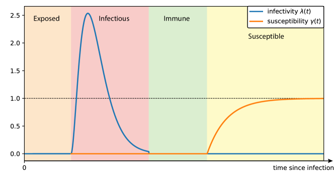
Figure 1. Illustration of a typical realization of the random infectivity and susceptibility functions of an individual from the time of infection to the time of recovery, and then to the time of losing immunity and becoming fully susceptible (or in general, partially susceptible).

In this paper, we propose a general stochastic epidemic model which takes into account a random infectivity and a random and gradual loss of immunity. See Figure 1 for a random realization of the infectivity and susceptibility of an individual after an infection. Individuals experience the susceptible-infected-immune-susceptible cycle. When an individual becomes infected, the infected period may include a latent exposed period and then an infectious period. Once an individual recovers from the infection, after some potential immune period (whose duration can be zero), the immunity is gradually lost, and the individual progressively becomes susceptible again. Then the individual may become infected again, and repeat the process at each new infection with a different realization of the random infectivity and susceptibility functions. This model can be regarded as a generalized SIS model. When “I” is interpreted as “infected” including exposed and infectious periods, and “S” is interpreted as including immune and susceptible periods. It can of course also be regarded as a generalized SEIS, SIRS or SEIRS model.

We prove in Theorem 3.2 that the pair of the average susceptibility and force of infectivity converges, when the size of the population goes to infinity, to a deterministic limiting model given by a system of integral equations depending on the law of the susceptibility and on the average of the infectivity function. This system generalizes the model of Kermack and McKendrick and in Section 5, we show how our model reduces to the Kermack and McKendrick PDE model under a special set of susceptibility and infectivity random functions and initial conditions. Indeed, in [19, 20] the functions of infectivity and susceptibility are deterministic and the same for all the individuals whereas in the present paper they are random and different for each individual.

We then obtain a characterization of the threshold of endemicity which depends on the law of susceptibility and not only on the mean, and which generalizes that of Kermack and McKendrick. We also give partial answers regarding the stability of the equilibria. More precisely, in Theorem 4.1 we prove the global asymptotical stability of the disease-free steady state when the basic reproduction number is lower than the above-mentioned threshold. We next characterize in Theorem 4.2 the endemic equilibrium when the basic reproduction number is larger than this threshold, and under additional assumptions we prove in Lemma 4.1 that the disease-free-steady state is unstable.

To prove these results, we will represent the epidemic as a system of interacting counting processes and use the tools of the theory of propagation of chaos, see Sznitman [27]. More precisely, our approach to prove the convergence result is to compare the processes counting the number of infections of each individual to a family of independent and identically distributed counting processes with a well-chosen coupling, following the method introduced in [6]. This approach is different from the techniques classically used for age-structured population models, as in [24, 17, 28, 11, 12, 8]. In these papers, the authors describe the model as a branching process (sometimes with interaction), Markovian in the age structure, in which the lifespan, birth rate and death rate depend on the age of all individuals in the population and where the process describing the ages of the various individuals is measure-valued. These works combine stochastic calculus and Markov process analysis in order to derive the limit model. The approach of the present paper is also different from the techniques used in the recent works [10, 25] which treat related epidemic models without loss of immunity. Indeed, in [25] the authors define a non–Markovian SIR model where the law of infectious period is arbitrary but the infectivity rate is constant and in [10] the authors replace the constant infectivity by a random infectivity function. The approach used in those papers combines stochastic calculus and the properties of Poisson random measures to establish the limit model, but it does not seem to be applicable in the setting of the present paper. Moreover, our approach with the coupling argument allows us to make weaker assumptions on the infectivity function than in [10].

Using random infectivity and susceptibility functions allows us to build a very general model which is both versatile and tractable. It captures the effect of a progressive loss of immunity when this loss is allowed to be very different from one individual to another. The integral equations that we obtain to describe the large population limit of our model are both compact and extremely general, since most epidemic model with homogeneous mixing and a fixed population size can be written under this form, no matter how many compartments are considered. The consequences of the variability of susceptibility on the endemic threshold have received very little attention in the literature, despite some profound implications which we outline in the present work. The fact that the threshold depends on the harmonic mean of the susceptibility reached after an infection shows that the heterogeneity of immune responses in real populations should not be neglected in public health decisions. Similarly, the variability of the immune response after vaccination (both in time and between individuals) should affect the efficacy of vaccination policies in non-trivial ways, although these questions are outside the scope of the present work.

Organization of the paper

The rest of the paper is organized as follows. In Section 2, we define the model in detail. In Section 3, we state the assumptions and the functional law of large numbers (FLLN) and discuss how the results reduce to the known results for the classical SIS and SIRS models. The results on the endemic equilibrium are presented in Section 4. In Section 5, we focus on the generalized SIRS model with a particular set of infectivity and susceptibility random functions and initial conditions, and show how the limit relates to the Kermack and McKendrick PDE model with the corresponding infection-age dependent infectivity and recovery-age dependent susceptibility. The proofs for the FLLN are given in Section 6 and those for the endemic equilibria in Section 7.

Notation

Throughout the paper, all the random variables and processes are defined on a common complete probability space $(\Omega,\mathcal{F},\mathbb{P})$. We use $\xrightarrow[N\to+\infty]{\mathbb{P}}$ to denote convergence in probability as the parameter $N\to\infty$. Let $\mathbb{N}$ denote the set of natural numbers and $\mathbb{R}^{k}(\mathbb{R}^{k}_{+})$ the space of $k$-dimensional vectors with real (nonnegative) numbers, with $\mathbb{R}(\mathbb{R}_{+})$ for $k=1$. We use $\mathds{1}_{\{\cdot\}}$ for the indicator function. Let $D=D(\mathbb{R}_{+};\mathbb{R})$ be the space of $\mathbb{R}$-valued càdlàg functions defined on $\mathbb{R}_{+}$, with convergence in $D$ meaning convergence in the Skorohod $J_{1}$ topology (see, e.g., [1, Chapter 3]). Also, we use $D^{k}$ to denote the $k$-fold product with the product $J_{1}$ topology. Let $C$ be the subset of $D$ consisting of continuous functions and $D_{+}$ the subset of $D$ of càdlàg functions with values on $\mathbb{R}_{+}$

2. Model description

We consider a population with fixed size $N\geq 1$. Initially, a random number of individuals within the population are chosen to be infected, while the others are assumed to be susceptible. Each individual is characterized by its current infectivity and susceptibility. The infectivity corresponds to the instantaneous rate at which an individual has a potentially infectious contact with another individual in the population, which is assumed to be chosen uniformly in the population. The latter then becomes infected with a probability equal to its current susceptibility (which will be assumed to be in $[0,1]$). At each new successful infection, the newly infected individual draws a random pair of functions $(\lambda,\gamma)$ following a given distribution, and, as long as this individual is not infected again, its infectivity (resp. susceptibility) will be given by $\lambda(t-\tau)$ (resp. $\gamma(t-\tau)$), where $\tau$ is the time at which the infection has happened. We shall assume that an individual cannot be infectious and susceptible at the same time. More precisely, the susceptibility of an individual must remain equal to zero as long as the infectivity function resulting from this individual’s latest infection has not vanished, see Assumption 2.1 below.

2.1. Notations

The infection process is described by a system of counting processes $(A^{N}_{k}(t),t\geq 0,1\leq k\leq N)$ where $A^{N}_{k}(t)$ counts the number of times that the $k$-th individual has been infected up to time $t$ (apart from its initial infection if the $k$-th individual is among the initially infected individuals).

Let $\{(\lambda_{k,i},\gamma_{k,i}),i\geq 1,1\leq k\leq N\}$ be a collection of i.i.d. $D^{2}$-valued random variables. $\lambda_{k,i}(t)$ (resp. $\gamma_{k,i}(t)$) is the infectivity (resp. susceptibility) of the $k$-th individual, $t$ units of time after its $i$-th infection, provided this individual has not already been infected again at this time.

Also let $\{(\lambda_{k,0},\gamma_{k,0}),1\leq k\leq N\}$ be a collection of i.i.d. $D^{2}$-valued random variables such that $0\leq\lambda_{k,0}(t)\leq\lambda_{*}$ and $0\leq\gamma_{k,0}(t)\leq 1$ for all $t\geq 0$ almost surely, independent from the previous one. Similarly, $\lambda_{k,0}(t)$ (resp. $\gamma_{k,0}(t)$) is the infectivity (resp. susceptibility) of the $k$-th individual at time $t$ if this individual has not already been infected on the interval $(0,t]$. Note that, typically, we shall assume that, at time zero, some fraction of the individuals are “susceptible”, hence $\mathbb{P}(\lambda_{k,0}\equiv 0)>0$. In addition, as in [10], an individual that is infectious at time zero may not have the same remaining infectious period (and infectivity) as an individual who has just been infected (to reflect the fact that it has been infected at some time in the past). As a result the pair $(\lambda_{k,0},\gamma_{k,0})$ is a priori not distributed as $(\lambda_{k,i},\gamma_{k,i})$ for $i\geq 1$, but its distribution can in principle remain quite general. We give more concrete constructions of the sequence $\{(\lambda_{k,0},\gamma_{k,0}),1\leq k\leq N\}$ in Remark 2.1 and in Assumption 4.1.

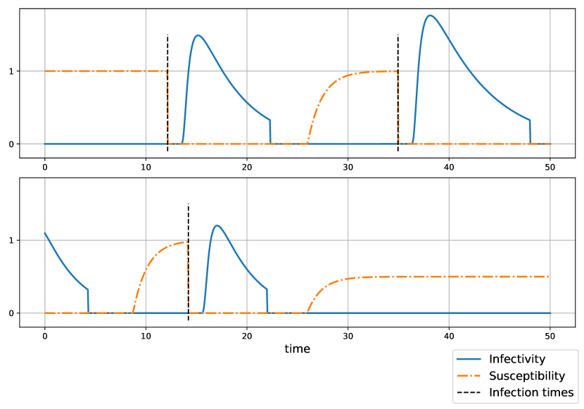
Figure 2. Illustration of the evolution of an individual’s infectivity and susceptibility through time. Each graphic shows the dynamics of an individual’s infectivity (blue) and susceptibility (orange). The top graphic corresponds to an individual which is initially susceptible, and the bottom one to an initially infectious individual. Note that, after being reinfected, the second individual remains partially immune even a long time after infection.

Recall that $A^{N}_{k}(t)$ denotes the number of times that the $k$-th individual has been (re-)infected on the interval $(0,t]$. Hence, the time elapsed since this individual’s last infection (or since time 0 if no such infection has occurred), is given by

$$\varsigma^{N}_{k}(t):=t-\left(\sup\{s\in(0,t]:A^{N}_{k}(s)=A^{N}_{k}(s^{-})+1\}\vee 0\right),$$

where we use the convention $\sup\emptyset=-\infty$. With this notation, the current infectivity and susceptibility of the $k$-th individual are given by

$$\lambda_{k,A^{N}_{k}(t)}(\varsigma^{N}_{k}(t)), \gamma_{k,A^{N}_{k}(t)}(\varsigma^{N}_{k}(t)).$$ and

Figure 2 shows a realisation of these processes for two individuals. Let us then define $\overline{\mathfrak{F}}^{N}(t)$ and $\overline{\mathfrak{S}}^{N}(t)$ as the average infectivity and susceptibility in the population, i.e.,

$$\overline{\mathfrak{F}}^{N}(t):=\frac{1}{N}\sum_{k=1}^{N}\lambda_{k,A_{k}^{N}(t)}(\varsigma^{N}_{k}(t)), \overline{\mathfrak{S}}^{N}(t):=\frac{1}{N}\sum_{k=1}^{N}\gamma_{k,A_{k}^{N}(t)}(\varsigma^{N}_{k}(t)).$$

According to our informal description of the model, the instantaneous rate at which the $\ell$-th individual infects the $k$-th individual is

$$\frac{1}{N}\lambda_{\ell,A^{N}_{\ell}(t)}(\varsigma^{N}_{\ell}(t))\gamma_{k,A^{N}_{k}(t)}(\varsigma^{N}_{k}(t))$$

where the $\frac{1}{N}$ factor comes from the probability that the $k$-th individual is chosen as the target of the infectious contact. Summing over the index $\ell$, the instantaneous rate at which the $k$-th individual is infected or reinfected is given by

$$\Upsilon_{k}^{N}(t):=\gamma_{k,A^{N}_{k}(t)}(\varsigma^{N}_{k}(t))\,\overline{\mathfrak{F}}^{N}(t).$$ (2.1)

This leads to the following formal definition of our model.

2.2. Definition of the model

Let $\{(\lambda_{k,i},\gamma_{k,i}),i\geq 1,1\leq k\leq N\}$ and $\{(\lambda_{k,0},\gamma_{k,0}),1\leq k\leq N\}$ be two independent families of i.i.d. random variables as above. Also let $(Q_{k},1\leq k\leq N)$ be an i.i.d. family of standard Poisson random measures on $\mathbb{R}_{+}^{2}$, also independent from the two previous families. The family of counting processes $(A^{N}_{k}(t),t\geq 0,1\leq k\leq N)$ is then defined as the solution of

$$A^{N}_{k}(t)=\int_{[0,t]\times\mathbb{R}_{+}}\mathds{1}_{u\leq\Upsilon^{N}_{k}(r^{-})}Q_{k}(dr,du),$$ (2.2)

where $\Upsilon_{k}^{N}$ is defined by (2.1).

Assumption 2.1.

We assume that there exists a constant $\lambda_{*}<\infty$ such that $0\leq\lambda_{k,i}(t)\leq\lambda_{*}$ almost surely, and that $0\leq\gamma_{k,i}(t)\leq 1$ for all $t\geq 0$, for all $i\geq 0$ and $1\leq k\leq N$, almost surely. Moreover

$$\sup\{t\geq 0,\,\lambda_{k,i}(t)>0\}\leq\inf\{t\geq 0,\,\gamma_{k,i}(t)>0\},$$ (2.3)

almost surely for all $1\leq k\leq N$ and $i\geq 0$.

We define, for $i\geq 0$ and $1\leq k\leq N$,

$$\eta_{k,i}:=\sup\{t\geq 0:\lambda_{k,i}(t)>0\}.$$

Assumption 2.1 ensures that the family $(A^{N}_{k}(t),t\geq 0,1\leq k\leq N)$ is well defined, since the instantaneous rate at which an infection takes place in the population is bounded by $\lambda_{*}N$ almost surely.

Condition (2.3) implies that, as long as an individual remains infectious (i.e. as long as $\varsigma^{N}_{k}(t)<\eta_{k,A^{N}_{k}(t)}$), he or she cannot be infected. Hence in each infectious-immune-susceptible cycle, the infectious and susceptible periods do not overlap. Note that (2.3) is not necessary for the process to be well defined, and we discuss the consequences of removing this assumption in Remark 3.3.

2.3. Number of infectious and uninfectious individuals

For $i\geq 1$, $\eta_{k,i}$ is the duration of the infectious period of the $k$-th individual following its $i$-th infection, while $\eta_{k,0}=0$ if the $k$-th individual is initially susceptible and $\eta_{k,0}>0$ is the remaining infectious period of the $k$-th individual if it is initially infectious. We shall say that the $k$-th individual is currently infectious (resp. uninfectious) if $\varsigma^{N}_{k}(t)<\eta_{k,A^{N}_{k}(t)}$ (resp. $\varsigma^{N}_{k}(t)\geq\eta_{k,A^{N}_{k}(t)}$). Note that, with this definition, an individual may be called infectious even if its current infectivity is equal to zero, for example during an exposed period. In the same way, an individual is called uninfectious if it is no longer infectious or has never been infected, hence this group comprises both recovered and susceptible individuals. This choice of two broadly defined compartments allows us to keep the notations tractable, but the equations obtained below can be generalized in a straightforward way to keep track of the number of individuals at different stages of their infection and susceptibility in more detail.

Let $I^{N}(t)$ (resp. $U^{N}(t)$) denote the number of infectious (resp. uninfectious) individuals in the population at time $t\geq 0$. Then

$$I^{N}(t)=\sum_{k=1}^{N}\mathds{1}_{\varsigma^{N}_{k}(t)<\eta_{k,A^{N}_{k}(t)}}, U^{N}(t)=\sum_{k=1}^{N}\mathds{1}_{\varsigma^{N}_{k}(t)\geq\eta_{k,A^{N}_{k}(t)}}.$$ and (2.4)

Note that, quite obviously, $U^{N}(t)+I^{N}(t)=N$ for all $t\geq 0$. We then define

$$\overline{I}(0):=\mathbb{P}(\eta_{1,0}>0), \overline{U}(0):=\mathbb{P}(\eta_{1,0}=0)=1-\overline{I}(0).$$

Recall that $\{(\lambda_{k,0},\gamma_{k,0}),1\leq k\leq N\}$, and hence $(\eta_{k,0},1\leq k\leq N)$, are independent and identically distributed. Thus by the law of large numbers,

$$\left(\frac{1}{N}I^{N}(0),\frac{1}{N}U^{N}(0)\right)=\left(\frac{1}{N}\sum_{k=1}^{N}\mathds{1}_{\eta_{k,0}>0},\frac{1}{N}\sum_{k=1}^{N}\mathds{1}_{\eta_{k,0}=0}\right)\to\left(\overline{I}(0),\overline{U}(0)\right)$$

almost surely as $N\to\infty$.

Remark 2.1.

The classical compartmental models

Most compartmental epidemic models can be obtained as special cases of our model, as long as no population structure is assumed. Here are a few examples.

1. The SIS model considers that infected individual instantly become infectious with some infectivity $\lambda$, and remain infectious for a random time $\eta$, after which they become instantly susceptible again. Thus, this model is obtained by assuming that, for $i\geq 1$,

   $$\lambda_{k,i}(t)=\lambda\mathds{1}_{0\leq t<\eta_{k,i}}, \gamma_{k,i}(t)=\mathds{1}_{t\geq\eta_{k,i}},$$ (2.5)

   and $\eta_{k,i}$ are non-negative random variables, which follow an exponential distribution in the case of the Markov model. Let us also specify the distribution of $(\lambda_{k,0},\gamma_{k,0})$. For this, fix $\overline{I}(0)\in[0,1]$, set $\overline{S}(0)=1-\overline{I}(0)$ and let $(\chi_{k},1\leq k\leq N)$ be a sequence of i.i.d. random variables taking values in $\{S,I\}$ such that $\mathbb{P}(\chi_{k}=S)=\overline{S}(0)$ and $\mathbb{P}(\chi_{k}=I)=\overline{I}(0)$. Then set

   $$\lambda_{k,0}(t)=\begin{cases}0&\text{ if }\chi_{k}=S,\\ \lambda\mathds{1}_{0\leq t<\eta_{k,0}}&\text{ if }\chi_{k}=I,\end{cases} \gamma_{k,0}(t)=\begin{cases}1&\text{ if }\chi_{k}=S,\\ \mathds{1}_{t\geq\eta_{k,0}}&\text{ if }\chi_{k}=I,\end{cases}$$ (2.6)

   where $(\eta_{k,0},1\leq k\leq N)$ is a sequence of i.i.d. positive random variables (which follow exponential distributions in the case of the Markov model). (Note that, with this definition, the model starts from a random initial condition, which is not always assumed in the literature, but does not greatly affect its behaviour.)

2. The SIR model instead considers that, at the end of the infectious period, infected individuals recover from the disease, and can no longer be infected again. This model can be obtained from the above by proceeding as for the SIS model, but assuming instead that

   $$\forall t\geq 0,i\geq 1,\quad\gamma_{k,i}(t)=0, \gamma_{k,0}(t)=\begin{cases}1&\text{ if }\chi_{k}=S,\\ 0&\text{ if }\chi_{k}=I.\end{cases}$$ and (2.7)

   Note that, in this case, if we keep a general distribution for $\lambda_{k,i}$ and $\lambda_{0,i}$, this model reduces to the one studied in [10].

3. The SIRS model assumes that, at the end of their infectious period, individuals stay immune to the disease for a random time $\theta$, after which they become fully susceptible again. This model is obtained by assuming that, for $i\geq 1$,

   $$\lambda_{k,i}(t)=\lambda\mathds{1}_{0\leq t<\eta_{k,i}}, \gamma_{k,i}(t)=\mathds{1}_{t\geq\eta_{k,i}+\theta_{k,i}},$$ (2.8)

   where $\{(\eta_{k,i},\theta_{k,i}),1\leq k\leq N,i\geq 1\}$ is a family of i.i.d. random variables taking values in $\mathbb{R}_{+}^{2}$ (which are distributed as pairs of independent exponential variables in the Markov models). The generalization of the definition of the distribution of $(\lambda_{k,0},\gamma_{k,0})$ to this case is straightforward.

   Note that, in the last two cases, the quantity $U^{N}(t)$ defined in (2.4) counts both susceptible and removed individuals. The actual number of susceptible and removed individuals in the SIRS model is given by

   $$S^{N}(t):=\sum_{k=1}^{N}\mathds{1}_{\eta_{k,A^{N}_{k}(t)}+\theta_{k,A^{N}_{k}(t)}\leq\varsigma^{N}_{k}(t)}, R^{N}(t):=\sum_{k=1}^{N}\mathds{1}_{\eta_{k,A^{N}_{k}(t)}\leq\varsigma^{N}_{k}(t)<\eta_{k,A^{N}_{k}(t)}+\theta_{k,A^{N}_{k}(t)}}.$$ (2.9)

   In the SIR model, the above expression remains exact provided we set $\theta_{k,i}=+\infty$ for $i\geq 1$, $\theta_{k,0}=0$ if $\chi_{k}=S$ and $\theta_{k,0}=+\infty$ if $\chi_{k}=I$.

It is also common to assume that infected individuals do not become infectious right after being infected, but first become exposed (i.e. infected but not yet infectious) before becoming infectious. This results in an additional compartment E, which can also be included in the above examples without difficulty.

Remark 2.2.

In [6], Chevallier studied a related model formulated as a system of age-dependent random Hawkes processes. This model considers a system of $N$ neurons which fire at a rate depending both on the times of the previous firings of other neurons and on the time elapsed since their last firing (called the age process). The author proves in [6] a propagation of chaos result for the empirical measure of the point processes corresponding to the firing times of the neurons, and for the empirical measure of the age processes of the neurons, as $N$ tends to infinity. Although neither our model or that of Chevallier can be formulated as a special case of the other, the two are closely related (if firing is understood as an analogous of being infected). The main difference between the two frameworks is in the assumptions on the randomness in the interaction between individuals after each firing/infection. For instance, our model would be closer to that of Chevallier if, instead of choosing a different infectivity function after each infection for each individual, we chose a different infectivity function for each directed pair of individuals at the beginning, and kept the same infectivity function for this pair of individual after each infection. Thus, the law of large numbers limit that we prove below can be seen as an extension of Chevallier result, and indeed some steps of the proof are adapted from [6]. See also Theorem 6.1 in Section 6 whose formulation is closer to the propagation of chaos result of [6]. In [5], the same author also proves a central limit theorem for the empirical measures mentioned above, something which we do not do here, but could be the subject of future work.

3. Functional law of large numbers

In this section we present the FLLN for the scaled processes $\big{(}\overline{\mathfrak{S}}^{N},\overline{\mathfrak{F}}^{N},\overline{U}^{N},\overline{I}^{N}\big{)}$ where $\overline{U}^{N}:=N^{-1}U^{N}$ and $\overline{I}^{N}:=N^{-1}I^{N}$.

Let

$$\overline{\lambda}_{0}(t):=\mathbb{E}\big{[}\lambda_{1,0}(t)\Big{|}\eta_{1,0}>0\big{]},\,\quad\overline{\lambda}(t):=\mathbb{E}\left[\lambda_{1,1}(t)\right],$$

$$F^{c}_{0}(t):=\mathbb{P}\left(\eta_{1,0}>t\big{|}\eta_{1,0}>0\right),\quad F^{c}(t):=\mathbb{P}\left(\eta>t\right),$$

and recall that $\overline{I}(0)=\mathbb{P}\left(\eta_{1,0}>0\right)$. Let $\mu$ and $\mu_{0}$ be the laws of $\gamma_{1,1}$ and $\gamma_{1,0}$ in $\mathcal{P}(D)$, respectively. For simplicity, we write $\gamma$ and $\gamma_{0}$ as processes with the same laws as $\gamma_{1,1}$ and $\gamma_{1,0}$, respectively.

To describe the limits of the FLLN, we introduce the following two-dimensional integral equations. Observe that the solution $(x,y)$ of this system depend on the laws of $(\lambda,\gamma)$ and $(\lambda_{0},\gamma_{0})$ only through expectations but for $\gamma$ and $\gamma_{0}$ it is much more complex.

We consider the following system of integral equations for which we look for a solution $(x,y)\in D^{2}_{+}$ :

$$x(t)=\mathbb{E}\left[\gamma_{0}(t)\exp\left(-\int_{0}^{t}\gamma_{0}(r)y(r)dr\right)\right]$$

$$\qquad\qquad+\int_{0}^{t}\mathbb{E}\left[\gamma(t-s)\exp\left(-\int_{s}^{t}\gamma(r-s)y(r)dr\right)\right]x(s)y(s)ds,$$ (3.1)

$$y(t)=\overline{I}(0)\overline{\lambda}_{0}(t)+\int_{0}^{t}\overline{\lambda}(t-s)x(s)y(s)ds.$$ (3.2)

In (3.1) we take the expectation on the law of $\gamma_{0}$ and $\gamma$ respectively.

Remark 3.1.

If the pair $(x,y)$ is a solution of set of equations (3.1)-(3.2), then for all $t\geq 0$,

$$\mathbb{E}\left[\exp\left(-\int_{0}^{t}\gamma_{0}(r)y(r)dr\right)\right]+\int_{0}^{t}\mathbb{E}\left[\exp\left(-\int_{s}^{t}\gamma(r-s)y(r)dr\right)\right]x(s)y(s)ds=1.$$ (3.3)

Indeed, we can note that, if we multiply the equation for $x(t)$ by $y(t)$, we obtain

$$y(t)x(t)=\mathbb{E}\left[y(t)\gamma_{0}(t)\exp\left(-\int_{0}^{t}\gamma_{0}(r)y(r)dr\right)\right]\\ +\int_{0}^{t}\mathbb{E}\left[y(t)\gamma(t-s)\exp\left(-\int_{s}^{t}\gamma(r-s)y(r)dr\right)\right]x(s)y(s)ds.$$

As a result,

$$\frac{d}{dt}\left(\mathbb{E}\left[\exp\left(-\int_{0}^{t}\gamma_{0}(r)y(r)dr\right)\right]+\int_{0}^{t}\mathbb{E}\left[\exp\left(-\int_{s}^{t}\gamma(r-s)y(r)dr\right)\right]x(s)y(s)ds\right)=0.$$

Integrating between 0 and t, we obtain the result.

Our first result establishes existence and uniqueness of the solution $(x,y)$ of (3.1)-(3.2). The proof is given in Section 6.

Theorem 3.1.

The set of equations (3.1)–(3.2) has a unique solution $(\overline{\mathfrak{S}},\overline{\mathfrak{F}})\in D^{2}(\mathbb{R}_{+},\mathbb{R}_{+})$. The solution belongs to $C^{2}(\mathbb{R}_{+})$ if $t\mapsto(\gamma_{0}(t),\overline{\lambda}_{0}(t))$ is continuous.

We have the following convergence result which proof in Section 6.

Theorem 3.2.

Under Assumption 2.1,

$$(\overline{\mathfrak{S}}^{N},\overline{\mathfrak{F}}^{N})\xrightarrow[N\to+\infty]{\mathbb{P}}(\overline{\mathfrak{S}},\overline{\mathfrak{F}})\quad\text{ in }\quad D^{2}$$ (3.4)

where $(\overline{\mathfrak{S}},\overline{\mathfrak{F}})$ is the unique solution of the system of equations (3.1)–(3.2).

Given the solution $(\overline{\mathfrak{S}},\overline{\mathfrak{F}})$,

$$(\overline{U}^{N},\overline{I}^{N})\xrightarrow[N\to+\infty]{\mathbb{P}}(\overline{U},\overline{I})\quad\text{ in }\quad D^{2}$$

where $(\overline{U},\overline{I})$ is given by

$$\overline{U}(t) =\mathbb{E}\left[\mathds{1}_{t\geq\eta_{0}}\exp\left(-\int_{0}^{t}\gamma_{0}(r)\overline{\mathfrak{F}}(s)dr\right)\right]$$

$$\qquad+\int_{0}^{t}\mathbb{E}\left[\mathds{1}_{t-s\geq\eta}\exp\left(-\int_{s}^{t}\gamma(r-s)\overline{\mathfrak{F}}(r)dr\right)\right]\overline{\mathfrak{S}}(s)\overline{\mathfrak{F}}(s)ds\,,$$ (3.5)

$$\overline{I}(t) =\overline{I}(0)F^{c}_{0}(t)+\int_{0}^{t}F^{c}(t-s)\overline{\mathfrak{S}}(s)\overline{\mathfrak{F}}(s)ds\,.$$ (3.6)

We note that

$$\overline{\mathfrak{S}}(t)=\mathbb{E}\left[\gamma_{0}(t)\exp\left(-\int_{0}^{t}\gamma_{0}(r)\overline{\mathfrak{F}}(r)dr\right)\right]$$

$$\qquad\qquad+\int_{0}^{t}\mathbb{E}\left[\gamma(t-s)\exp\left(-\int_{s}^{t}\gamma(r-s)\overline{\mathfrak{F}}(r)dr\right)\right]\overline{\mathfrak{S}}(s)\overline{\mathfrak{F}}(s)ds,$$ (3.7)

$$\overline{\mathfrak{F}}(t)=\overline{I}(0)\overline{\lambda}_{0}(t)+\int_{0}^{t}\overline{\lambda}(t-s)\overline{\mathfrak{S}}(s)\overline{\mathfrak{F}}(s)ds\,.$$ (3.8)

Remark 3.2.

Since $\overline{U}^{N}(t)+\overline{I}^{N}(t)=1$ for all $t\geq 0$ and $N\geq 1$, it follows from the above convergence that $\overline{U}(t)+\overline{I}(t)=1$ as well. Let us check that this follows also from the set of equations (3.5)-(3.6) satisfied by $(\overline{\mathfrak{S}},\overline{\mathfrak{F}})$.

First we note that, by (2.3) in Assumption 4.1, $\gamma(t)=0$ for all $t\in[0,\eta)$ and $\gamma_{0}(t)=0$ for $t\in(0,\eta_{0})$, hence

$$F_{0}^{c}(t)=\mathbb{E}\left[\mathds{1}_{t<\eta_{0}}\exp\left(-\int_{0}^{t}\gamma_{0}(r)\overline{\mathfrak{F}}(r)dr\right)\right], F^{c}(t-s)=\mathbb{E}\left[\mathds{1}_{t-s<\eta}\exp\left(\int_{s}^{t}\gamma(r-s)\overline{\mathfrak{F}}(r)dr\right)\right].$$

Hence, summing (3.5) and (3.6), we obtain

$$\overline{U}(t)+\overline{I}(t)=\mathbb{E}\left[\exp\left(-\int_{0}^{t}\gamma_{0}(r)\overline{\mathfrak{F}}(r)dr\right)\right]+\int_{0}^{t}\mathbb{E}\left[\exp\left(-\int_{s}^{t}\gamma(r-s)\overline{\mathfrak{F}}(r)dr\right)\right]\overline{\mathfrak{S}}(s)\overline{\mathfrak{F}}(s)ds.$$ (3.9)

Therefore, as $(\overline{\mathfrak{S}},\overline{\mathfrak{F}})$ is a solution of the set of equations (3.1)-(3.2), by Remark 3.1 we conclude that $\overline{U}(t)+\overline{I}(t)=1$ for all $t\geq 0$. Equation (3.3) should thus be seen as stating the conservation of the population size.

Remark 3.3.

Without condition $\eqref{eqq10}$ of Assumption 2.1, the limit obtained in the functional law of large numbers satisfies a different set of equations. More precisely, equation (3.8) is replaced by (3.10) and (3.6) by (3.11), where (3.10) and (3.11) are given below:

$$\overline{\mathfrak{F}}(t)=\mathbb{E}\left[\lambda_{0}(t)\exp\left(-\int_{0}^{t}\gamma_{0}(r)\overline{\mathfrak{F}}(r)dr\right)\right]$$

$$\qquad\qquad+\int_{0}^{t}\mathbb{E}\left[\lambda(t-s)\exp\left(-\int_{s}^{t}\gamma(r-s)\overline{\mathfrak{F}}(r)dr\right)\right]\overline{\mathfrak{S}}(s)\overline{\mathfrak{F}}(s)ds,$$ (3.10)

$$\overline{I}(t)=\mathbb{E}\left[\mathds{1}_{\eta_{0}>t}\exp\left(-\int_{0}^{t}\gamma_{0}(r)\overline{\mathfrak{F}}(s)dr\right)\right]$$

$$\qquad\qquad+\int_{0}^{t}\mathbb{E}\left[\mathds{1}_{\eta>t-s}\exp\left(-\int_{s}^{t}\gamma(r-s)\overline{\mathfrak{F}}(r)dr\right)\right]\overline{\mathfrak{S}}(s)\overline{\mathfrak{F}}(s)ds\,.$$ (3.11)

Remark 3.4.

We can check that, in the special cases mentioned in Remark 2.1, the limiting system of equations obtained in Theorem 3.2 coincides with the corresponding models in the literature.

1. In the case of the SIS model, we note that, by (2.5) and (2.6),

   $$\overline{\lambda}(t)=\lambda\mathbb{P}(\eta>t), \overline{\lambda}_{0}(t)=\lambda\mathbb{P}(\eta_{0}>t\,|\,\eta_{0}>0).$$

   It thus follows from (3.8) and (3.6) that $\overline{\mathfrak{F}}(t)=\lambda\overline{I}(t)$ for all $t\geq 0$. Moreover, comparing (3.7) and (3.5) and using (2.5) and (2.6), we see that $\overline{\mathfrak{S}}(t)=\overline{U}(t)$. Combining this with the fact that $\overline{I}(t)+\overline{U}(t)=1$, we obtain

   $$\overline{I}(t)=\overline{I}(0)F^{c}_{0}(t)+\lambda\int_{0}^{t}F^{c}(t-s)(1-\overline{I}(s))\overline{I}(s)ds,$$ (3.12)

   as stated in Theorem 2.3 of [25].

2. In the case of the SIR model, from the definition of $\gamma$ and $\gamma_{0}$ in (2.7) and (3.7), we see that

   $$\overline{\mathfrak{S}}(t)=\overline{S}(0)\exp\left(-\int_{0}^{t}\overline{\mathfrak{F}}(r)dr\right)\quad\text{ and }\quad\overline{U}(t)=\overline{\mathfrak{S}}(t)+\overline{R}(t).$$

   Combined with the fact that $\overline{\mathfrak{F}}(t)=\lambda\overline{I}(t)$, this yields the statement of Theorem 2.1 in [25].

3. In the case of the SIRS model, we note that, in view of (2.7), $\overline{U}(t)=\overline{S}(t)+\overline{R}(t)$, where

   $$\overline{S}(t)=\mathbb{E}\left[\mathds{1}_{\eta_{0}+\theta_{0}\leq t}\exp\left(-\int_{0}^{t}\gamma_{0}(r)\overline{\mathfrak{F}}(r)dr\right)\right]\\ +\int_{0}^{t}\mathbb{E}\left[\mathds{1}_{\eta+\theta\leq t-s}\exp\left(-\int_{s}^{t}\gamma(r-s)\overline{\mathfrak{F}}(r)dr\right)\right]\overline{\mathfrak{S}}(s)\overline{\mathfrak{F}}(s)ds,$$

   and

   $$\overline{R}(t)=\mathbb{E}\left[\mathds{1}_{\eta_{0}\leq t<\eta_{0}+\theta_{0}}\exp\left(-\int_{0}^{t}\gamma_{0}(r)\overline{\mathfrak{F}}(r)dr\right)\right]\\ +\int_{0}^{t}\mathbb{E}\left[\mathds{1}_{\eta\leq t-s<\eta+\theta}\exp\left(-\int_{s}^{t}\gamma(r-s)\overline{\mathfrak{F}}(r)dr\right)\right]\overline{\mathfrak{S}}(s)\overline{\mathfrak{F}}(s)ds.$$

   In fact, $\overline{S}$ and $\overline{R}$ are the limit of $\frac{1}{N}S^{N}$ and $\frac{1}{N}R^{N}$, respectively, where $S^{N}$ and $R^{N}$ are defined in (2.9) (recall that, for simplicity, we assumed that no individual is initially in the R compartment). But, from the definition of $\gamma$ in (2.8), $\gamma(t)=0$ for all $t\in[\eta,\eta+\theta)$ and $\gamma_{0}(t)=0$ for all $t\in[\eta_{0},\eta_{0}+\theta_{0})$, hence

   $$\overline{S}(t)=\overline{S}(0)\exp\left(-\int_{0}^{t}\overline{\mathfrak{F}}(r)dr\right)+\overline{I}(0)\mathbb{E}\left[\mathds{1}_{\eta_{0}+\theta_{0}\leq t}\exp\left(-\int_{\eta_{0}+\theta_{0}}^{t}\overline{\mathfrak{F}}(r)dr\right)\right]\\ +\int_{0}^{t}\mathbb{E}\left[\mathds{1}_{\eta+\theta\leq t-s}\exp\left(-\int_{s+\eta+\theta}^{t}\overline{\mathfrak{F}}(r)dr\right)\right]\overline{\mathfrak{F}}(s)\overline{\mathfrak{S}}(s)ds,$$

   and

   $$\overline{R}(t)=\overline{I}(0)\mathbb{P}(\eta_{0}\leq t<\eta_{0}+\theta_{0}\,|\,\eta_{0}>0)+\int_{0}^{t}\mathbb{P}(\eta\leq t-s<\eta+\theta)\overline{\mathfrak{F}}(s)\overline{\mathfrak{S}}(s)ds.$$

   Combined with $\overline{\mathfrak{F}}(t)=\lambda\overline{I}(t)$, $\overline{\mathfrak{S}}(t)=\overline{S}(t)$ and

   $$\overline{S}(t)+\overline{I}(t)+\overline{R}(t)=\overline{U}(t)+\overline{I}(t)=1,$$

   this yields the result stated in Theorem 3.3 in [25].

4. The endemic equilibrium

In this section we study the endemic equilibrium properties using the limits from the FLLN. We first recall the endemic equilibrium behavior of the classical SIS model discussed in Remark 2.1. Given the infectivity rate $\lambda$ and recovery rate $\beta:=(\mathbb{E}[\eta])^{-1}$, the basic reproduction number is given by $R_{0}=\lambda/\beta$. It is well known (see, e.g., [25, Section 4.3], and also [3] for a discussion on the Markovian model) that if $R_{0}\leq 1$, $\overline{I}(t)\to\overline{I}_{*}=0$ as $t\to\infty$, and if $R_{0}>1$ and $\overline{I}(0)>0,\,\overline{I}(t)\to\overline{I}_{*}=1-R_{0}^{-1}=1-\beta/\lambda$ as $t\to\infty$. This can be easily obtained from the expression of $\overline{I}(t)$ in (3.12). In words, in the case $R_{0}\leq 1$, the disease-free steady state is globally asymptotically stable, and in the case $R_{0}>1$, the disease-free steady state is unstable and there is exactly one endemic steady state, which is globally stable. Recall that in this model, $\overline{\lambda}(t)=\lambda F^{c}(t)$. Thus it is equivalent to write

$$R_{0}=\int_{0}^{\infty}\overline{\lambda}(t)dt\,,$$ (4.1)

since $\int_{0}^{\infty}F^{c}(t)dt=\beta^{-1}$. In fact, the expression of $R_{0}$ in (4.1) is the definition of the the basic reproduction number in the Kermack and McKendrick model with an average infectivity function $\overline{\lambda}(t)$, because it represents the average number of individuals infected by an infected individual in a fully susceptible population.

We make the following assumptions on the random susceptibility and infectivity functions in order to study the equilibria of our model.

Assumption 4.1.

The random functions $t\mapsto\gamma(t)$ and $t\mapsto\gamma_{0}(t)$ are non-decreasing a.s. Moreover the pair $(\lambda_{0},\gamma_{0})$ is distributed as follows. Let $(\tilde{\lambda},\tilde{\gamma},\tilde{\eta})$ be distributed as $(\lambda,\gamma,\eta)$ and let $\xi\geq 0$ be a random variable such that $\xi\leq\tilde{\eta}$ almost surely. Let $\chi$ be a Bernoulli random variable with $\mathbb{P}(\chi=1)=\overline{I}(0)$, independent from $(\tilde{\lambda},\tilde{\gamma},\tilde{\eta},\xi)$. Then

$$\lambda_{0}(t)=\begin{cases}0&\mbox{ if }\chi=0,\\ \tilde{\lambda}(t+\xi)&\mbox{ if }\chi=1.\end{cases}\quad\text{ and }\quad\gamma_{0}(t)=\begin{cases}1&\mbox{ if }\chi=0,\\ \tilde{\gamma}(t+\xi)&\mbox{ if }\chi=1.\end{cases}$$

The random variable $\xi$ represents the age of infection at time zero of the initially infectious individuals.

We define

$$\gamma_{\ast}:=\sup_{t\geq 0}\gamma(t)=\lim_{t\to+\infty}\gamma(t),\quad\text{ and }\quad\gamma_{0,*}:=\lim_{t\to+\infty}\gamma_{0}(t).$$

In the classical SIS model, the susceptibility functions $\gamma(t)=\mathds{1}_{t\geq\eta}$ and $\gamma_{0}(t)=\mathds{1}_{t\geq\eta_{0}}$ such that $\gamma_{*}=1$ a.s. However, after being infected and recovered, individuals lose immunity gradually and do not necessarily reach “full” susceptibility (being equal to 1). Thus, $\gamma_{\ast}$ may take any value in $[0,1]$ and is a priori random.

We find that the classification of the endemic equilibria depends on the law of $\gamma_{*}$, more specifically on whether $R_{0}$ is smaller than or larger than $\mathbb{E}[1/\gamma_{*}]$. Note that this expectation $\mathbb{E}[1/\gamma_{*}]$ may not be finite in general (for example if $\mathbb{P}(\gamma_{*}=0)>0$). We first prove the following equilibrium result under the condition that $R_{0}<\mathbb{E}[1/\gamma_{*}]$.

Theorem 4.1.

Under Assumption 4.1 and assuming $R_{0}<+\infty$, if $R_{0}<\mathbb{E}\left[1/\gamma_{*}\right],$ there exists $\overline{\mathfrak{S}}_{*}\in[0,1]$ such that

$$(\overline{\mathfrak{F}}(t),\overline{\mathfrak{S}}(t))\to(0,\overline{\mathfrak{S}}_{*})\quad as\quad t\to\infty,$$

where

$$\overline{\mathfrak{S}}_{\ast}=\lim_{t\to+\infty}\overline{\mathfrak{S}}(t) =\mathbb{E}\left[\gamma_{0,*}\exp\left(-\int_{0}^{+\infty}\gamma_{0}(r)\overline{\mathfrak{F}}(r)dr\right)\right]$$

$$\qquad+\int_{0}^{+\infty}\mathbb{E}\left[\gamma_{\ast}\exp\left(-\int_{s}^{+\infty}\gamma(r-s)\overline{\mathfrak{F}}(r)dr\right)\right]\overline{\mathfrak{S}}(s)\overline{\mathfrak{F}}(s)ds.$$ (4.2)

As a consequence, $(\overline{U}(t),\overline{I}(t))\to(\overline{U}_{*},\overline{I}_{*})$ as $t\to\infty$, where $\overline{U}_{*}=1$ and $\overline{I}_{*}=0$. In the special case $\gamma_{*}=1$ a.s., we also have $\overline{\mathfrak{S}}_{*}=1$.

Remark 4.1.

Without the assumption of the growth of the function $\gamma$, when $R_{0}<\mathbb{E}\left[\left(\sup_{t}\gamma(t)\right)^{-1}\right]$ the same proof as that of Theorem 4.1 shows that as $t\to+\infty,\,\overline{\mathfrak{F}}(t)\to 0$ and $\overline{I}(t)\to 0.$

Note that in this theorem, we do not assume $\mathbb{E}\left[1/\gamma_{*}\right]<+\infty$, however, we do assume that $R_{0}<\infty$, that is, $\overline{\lambda}(t)$ is integrable.

Remark 4.2.

In [15, Proposition $8.9$] one can find a similar result for a model with demography.

The case $R_{0}\geq\mathbb{E}[1/\gamma_{*}]$ is more complex. We make the following additional assumption.

Assumption 4.2.

There exists a non-negative random variable $t_{\ast}$ such that $\mathbb{E}\left[t_{\ast}\right]<+\infty$ and for $t\geq t_{\ast},\,\gamma(t)\geq\frac{\gamma_{\ast}}{2}$ a.s.

Theorem 4.2.

Suppose that Assumptions 4.1 and 4.2 hold and $R_{0}>\mathbb{E}\left[\frac{1}{\gamma_{*}}\right]$. If there exists $(\overline{\mathfrak{S}}_{\ast},\overline{\mathfrak{F}}_{\ast})$ such that $(\overline{\mathfrak{S}}(t),\overline{\mathfrak{F}}(t))\xrightarrow[t\to+\infty]{}(\overline{\mathfrak{S}}_{\ast},\overline{\mathfrak{F}}_{\ast})$, either $\overline{\mathfrak{S}}_{\ast}\in[0,1]$ and $\overline{\mathfrak{F}}_{\ast}=0$, or else

$$\overline{\mathfrak{S}}_{\ast}=\frac{1}{R_{0}}$$

and $\overline{\mathfrak{F}}_{\ast}$ is the unique positive solution of the equation

$$\int_{0}^{+\infty}\mathbb{E}\left[\exp\left(-\int_{0}^{s}\gamma\left(\frac{r}{\overline{\mathfrak{F}}_{\ast}}\right)dr\right)\right]ds=R_{0}.$$ (4.3)

In the second case, $(\overline{I}(t),\overline{U}(t))\to(\overline{I}_{*},\overline{U}_{*})$ as $t\to\infty$, where $\overline{U}_{*}=1-\overline{I}_{*}$ and

$$\overline{I}_{*}=\frac{\mathbb{E}\left[\eta\right]\overline{\mathfrak{F}}_{*}}{R_{0}}\,.$$ (4.4)

If $R_{0}=\mathbb{E}\left[\frac{1}{\gamma_{*}}\right]$, the same statement holds but (4.3) does not admit any positive solution, so, necessarily, $\overline{\mathfrak{F}}_{\ast}=0$ and thus $\overline{I}_{*}=0$.

Corollary 4.1.

Suppose that Assumptions 4.1 and 4.2 hold and $R_{0}>\mathbb{E}\left[\frac{1}{\gamma_{*}}\right]$. Assume that $\gamma(t)=\gamma_{\ast}\mathds{1}_{t\geq\zeta}$, where $\zeta$ is a random variable satisfying $\zeta\geq\eta$ almost surely and $\mathbb{E}[\zeta]<+\infty$ and $\gamma_{*}$ is a random variable taking values in $(0,1]$. Then,

$$\overline{\mathfrak{F}}_{\ast}=\frac{R_{0}-\mathbb{E}\left[\frac{1}{\gamma_{*}}\right]}{\mathbb{E}\left[\zeta\right]},$$ (4.5)

and

$$\overline{I}_{*}=\frac{\mathbb{E}[\eta]\overline{\mathfrak{F}}_{*}}{R_{0}}=\frac{\mathbb{E}[\eta]}{\mathbb{E}[\zeta]}\left(1-R_{0}^{-1}\mathbb{E}\left[\frac{1}{\gamma_{*}}\right]\right)$$ (4.6)

where $R_{0}$ is given in (4.1).

Proof.

In this case, equation (4.3) becomes

$$\int_{0}^{+\infty}\mathbb{E}\left[\exp\left(-\gamma_{\ast}\int_{0}^{s}\mathds{1}_{\frac{r}{\overline{\mathfrak{F}}_{\ast}}\geq\zeta}dr\right)\right]ds=R_{0}.$$

By a change of variables and Fubini’s theorem, the left hand side is equal to

$$\overline{\mathfrak{F}}_{\ast}\int_{0}^{+\infty}\mathbb{E}\left[\exp\left(-\overline{\mathfrak{F}}_{\ast}\gamma_{\ast}\int_{0}^{s}\mathds{1}_{r\geq\zeta}dr\right)\right]ds =\overline{\mathfrak{F}}_{\ast}\int_{0}^{+\infty}\mathbb{E}\left[\mathds{1}_{\zeta>s}+\mathds{1}_{\zeta\leq s}\exp\left(-\overline{\mathfrak{F}}_{\ast}\gamma_{\ast}(s-\zeta)dr\right)\right]ds$$

$$=\overline{\mathfrak{F}}_{*}\mathbb{E}\left[\zeta\right]+\overline{\mathfrak{F}}_{\ast}\mathbb{E}\left[\int_{\zeta}^{+\infty}\exp\left(-\overline{\mathfrak{F}}_{\ast}\gamma_{\ast}(s-\zeta)\right)ds\right]$$

$$=\overline{\mathfrak{F}}_{*}\mathbb{E}\left[\zeta\right]+\mathbb{E}\left[\frac{1}{\gamma_{*}}\right].$$

This gives the expression in (4.5). ∎

Remark 4.3.

For the classical models discussed in Remark 2.1, the above allows us to recover previously known results.

1. In the SIS model, we have $\gamma_{*}=1$ and $\eta=\zeta$ almost surely, so we obtain that $\overline{I}(t)\to 0$ as $t\to\infty$ if $R_{0}\leq 1$, and that, if $R_{0}>1$, the only other possible limit for $\overline{I}(t)$ is given by

   $$\overline{I}_{*}=\frac{\mathbb{E}[\eta]}{\mathbb{E}[\zeta]}\left(1-R_{0}^{-1}\mathbb{E}\left[\frac{1}{\gamma_{*}}\right]\right)=1-\frac{1}{R_{0}}.$$

2. For the SIRS model, we have $\gamma_{*}=1$ and $\zeta=\eta+\theta$. As a result, applying Corollary 4.1, we see that, when $R_{0}>1$, the only possible positive limit for $\overline{I}(t)$ is

   $$\overline{I}_{*}=\frac{\mathbb{E}[\eta]}{\mathbb{E}[\eta]+\mathbb{E}[\theta]}\left(1-\frac{1}{R_{0}}\right).$$

   In the same way, we can also deduce that $\overline{R}_{*}:=\lim_{t\to+\infty}\overline{R}(t)$ is given by

   $$\overline{R}_{*}=1-\overline{\mathfrak{S}}_{*}-\overline{I}_{*}=\frac{\mathbb{E}[\theta]}{\mathbb{E}[\eta]+\mathbb{E}[\theta]}\left(1-\frac{1}{R_{0}}\right).$$

   We refer to Proposition 4.2 of [25] for a previous derivation of this equilibrium in the case of a deterministic ODE model.

Our results in (4.5)–(4.6) thus extend those for classical compartmental models. Note that $\gamma_{*}$ is random and takes values in $[0,1]$, indicating potentially partial susceptibility after recovery.

For the SIS and SIRS models discussed in Remark 4.3, it is known that, if $R_{0}>1$ and $\overline{I}(0)>0$, then $\overline{I}(t)$ does indeed converge to the endemic equilibrium $\overline{I}_{*}$ as $t\to\infty$. We are not yet able to prove such a result for our general model. We can, however, prove that $\overline{\mathfrak{F}}(t)$ does not converge to zero as $t\to\infty$, under some additional assumptions.

Assumption 4.3.

$\gamma_{\ast}$ is deterministic and for any $\delta\in(0,1)$, there exists a deterministic $t_{\delta}>0$ such that

$$\gamma_{0}(t_{\delta})\wedge\gamma(t_{\delta})\geq(1-\delta)\gamma_{\ast}\text{ almost surely.}$$ (4.7)

Assumption 4.4.

There exists a positive decreasing function $h$ such that $h(0)=1$ and for all $s,t\in\mathbb{R}_{+},\;\overline{\lambda}(s+t)\geq h(s)\overline{\lambda}(t)$. The same holds for $\overline{\lambda}_{0}$. In addition, $\overline{\lambda}_{0}$ is continuous.

Remark 4.4.

Assumption 4.3 ensures that after some time the average of susceptibility returns to above $\frac{1}{R_{0}}$ if there is not too much re-infection and Assumption 4.4 ensures that the force of infection does not decrease too rapidly.

Lemma 4.1.

Under Assumptions 4.1–4.4, if $R_{0}>\mathbb{E}\left[\frac{1}{\gamma_{*}}\right]$ and $\overline{\mathfrak{F}}(0)>0$, then there exists $c>0$ such that for all $t>0,\,\overline{\mathfrak{F}}(t)\geq c.$

Remark 4.5.

Lemma 4.1 shows that under Assumptions 4.1–4.4, when $R_{0}>\mathbb{E}\left[\frac{1}{\gamma_{*}}\right]$ the disease free-steady state is unstable. A similar result was obtained by Inaba [15, Proposition $8.11$] for the model described in Section 5.

From Theorem 4.2 and Lemma 4.1, we can deduce the following result.

Corollary 4.2.

Under Assumptions 4.1–4.4 and assuming $R_{0}>\mathbb{E}\left[\frac{1}{\gamma_{*}}\right]$ and $\overline{\mathfrak{F}}(0)>0$, the result in Theorem 4.2 holds with $\overline{\mathfrak{S}}_{*}=1/R_{0}$ and $\overline{\mathfrak{F}}_{*}$ is the unique positive solution of (4.3). As a consequence, $(\overline{U}(t),\overline{I}(t))\to(\overline{U}_{*},\overline{I}_{*})$ as $t\to\infty$, where $\overline{U}_{*}=1-\overline{I}_{*}$ and

$$\overline{I}_{*}=\beta^{-1}\overline{\mathfrak{S}}_{*}\overline{\mathfrak{F}}_{*}=(\beta R_{0})^{-1}\overline{\mathfrak{F}}_{*}$$

with $\beta^{-1}=\mathbb{E}[\eta]$.

We make the following conjecture on the convergence to the equilibrium in the case $R_{0}>\mathbb{E}\left[1/\gamma_{*}\right]$.

Conjecture 4.1.

Under Assumptions 4.1–4.4, if $R_{0}>\mathbb{E}\left[\frac{1}{\gamma_{*}}\right]$ and $\overline{\mathfrak{F}}(0)>0$, then

$$(\overline{\mathfrak{F}}(t),\overline{\mathfrak{S}}(t))\to(\overline{\mathfrak{F}}_{*},\overline{\mathfrak{S}}_{*})\quad as\quad t\to\infty,$$

where $\overline{\mathfrak{S}}_{*}=1/R_{0}$ and $\overline{\mathfrak{F}}_{*}$ is the unique positive solution of (4.3).

This conjecture is equivalent to another. Indeed, by applying the Arzelà-Ascoli Theorem to the set of functions $\{(\tau_{j}\overline{\mathfrak{S}},\tau_{j}\overline{\mathfrak{F}}),\,j\in\mathbb{N}\}$ where $\tau_{j}x(t):=x(t+t_{j})$ and $(t_{j})_{j}\subset\mathbb{R}_{+},\,t_{j}\to+\infty$ as $j\to+\infty$, there exists a subsequence of pairs $(\tau_{j}\overline{\mathfrak{S}},\tau_{j}\overline{\mathfrak{F}})$ denoted again $(\tau_{j}\overline{\mathfrak{S}},\tau_{j}\overline{\mathfrak{F}})$ such that $(x_{j},y_{j}):=(\tau_{j}\overline{\mathfrak{S}},\tau_{j}\overline{\mathfrak{F}})\to(x,y)$ uniformly on compact sets as $j\to+\infty$. Note that the pair $(x_{j}(t),y_{j}(t))$ satisfies the following system of equations: for $t\geq-t_{j}$,

$$x_{j}(t)=\mathbb{E}\left[\gamma_{0}(t+t_{j})\exp\left(-\int_{0}^{t+t_{j}}\gamma_{0}(r)\overline{\mathfrak{F}}(r)dr\right)\right]$$

$$\qquad\qquad+\int_{-t_{j}}^{t}\mathbb{E}\left[\gamma(t-s)\exp\left(-\int_{s}^{t}\gamma(r-s)y_{j}(r)dr\right)\right]x_{j}(s)y_{j}(s)ds,$$ (4.8)

$$y_{j}(t)=\overline{I}(0)\overline{\lambda}_{0}(t+t_{j})+\int_{-t_{j}}^{t}\overline{\lambda}(t-s)x_{j}(s)y_{j}(s)ds.$$ (4.9)

As a result, as the first terms of the right hand side of (4.8) and (4.9) tend to zero when $j\to+\infty$, and $(x_{j}(t),y_{j}(t))\to(x(t),y(t))$ for all $t\in\mathbb{R}$, we deduce by the dominated convergence theorem that the pair $(x,y)$ satisfies the following set of equations,

$$y(t)=\int_{-\infty}^{t}\overline{\lambda}(t-s)x(s)y(s)ds,$$ (4.10)

$$\int_{-\infty}^{t}\mathbb{E}\left[\exp\left(-\int_{s}^{t}\gamma(r-s)y(r)dr\right)\right]x(s)y(s)ds=1.$$ (4.11)

We can remark that the constant pair $(\frac{1}{R_{0}},\overline{\mathfrak{F}}_{\ast})$ where $\overline{\mathfrak{F}}_{\ast}$ is the unique solution of (4.3) is a solution of (4.10)-(4.11). Hence if this solution is unique, all converging subsequences of $(\tau_{j}\overline{\mathfrak{S}},\tau_{j}\overline{\mathfrak{F}})$ have the same limit, from which we can easily conclude the convergence of $(\overline{\mathfrak{F}}(t),\overline{\mathfrak{S}}(t))$ as $t\to\infty$.

Thus, Conjecture 4.1 is equivalent to the following.

Conjecture 4.2.

Under Assumptions 4.1–4.4, if $R_{0}>\mathbb{E}\left[\frac{1}{\gamma_{*}}\right]$ and $\overline{\mathfrak{F}}(0)>0$, the set of equations (4.10)-(4.11) has a unique positive and bounded solution on $\mathbb{R}$.

5. Relating to the Kermack and McKendrick PDEs for the SIRS model

5.1. The FLLN limits with a special set of susceptibility/infectivity functions and initial conditions

We consider the special family of susceptibility and infectivity functions:

$$\lambda(t)=\widetilde{\lambda}(t)\mathds{1}_{t<\eta}\,\quad\text{ and }\quad\gamma(t)=\widetilde{\gamma}(t-\eta)\mathds{1}_{t>\eta}$$

where $\widetilde{\lambda}(t)$ and $\widetilde{\gamma}(t)$ are deterministic functions, representing the infectivity and susceptibility functions, and the infectious period $\eta$ is a random variable with cumulative distribution function $F$. Then we have $\overline{\lambda}(t)=\widetilde{\lambda}(t)F^{c}(t)$. In addition, let $f$ be the density function of $F$ and $\mu_{F}(t):=\frac{f(t)}{F^{c}(t)}$ be the hazard rate function of $F$. Then one can also write

$$F^{c}(t)=\exp\left(-\int_{0}^{t}\mu_{F}(s)ds\right),$$ (5.1)

For an initially infected individual, we recall that $\xi$ is the elapsed times since the individual was last infected before time zero. We also assume that the infectivity function of an initially infected individual is the same as that of a newly infected individual but shifted by the elapsed time since infection before time zero, that is,

$$\lambda_{0}(t)=\widetilde{\lambda}(t+\xi)\mathds{1}_{t<\eta_{0}}$$

where $\eta_{0}$ is the duration of the remaining infectious period after time zero, whose distribution depends on the elapsed infection time $\xi$. To specify the distribution of $\xi$, we assume that there exists a function $\overline{I}(0,\tau)$ such that $\overline{I}(0)=\int_{0}^{\infty}\overline{I}(0,\tau)d\tau$, that is, $\overline{I}(0,\tau)$ is the density of the distribution of $\overline{I}(0)$ over the ages of infection. Then we can specify the distribution of $\xi$ as

$$\mathbb{P}(\xi>x)=\frac{1}{\overline{I}(0)}\int_{x}^{+\infty}\overline{I}(0,r)dr.$$ (5.2)

And the conditional distribution of $\eta_{0}$ given $\xi$ is given by

$$\mathbb{P}(\eta_{0}>t\big{|}\xi)=\frac{F^{c}(\xi+t)}{F^{c}(\xi)}=\exp\left(-\int_{\xi}^{\xi+t}\mu_{F}(r)dr\right).$$ (5.3)

It is then clear that

$$\overline{\lambda}_{0}(t)=\mathbb{E}\left[\widetilde{\lambda}(t+\xi)\mathds{1}_{t<\eta_{0}}\right]=\frac{1}{\overline{I}(0)}\int_{0}^{+\infty}\widetilde{\lambda}(t+\tau)\overline{I}(0,\tau)\exp\left(-\int_{\tau}^{t+\tau}\mu_{F}(s)ds\right)d\tau\,.$$ (5.4)

Next, to specify the susceptibility $\gamma_{0}(t)$ associated with an individual, we consider the three groups of individuals at time zero, fully susceptible $\overline{S}(0)$, initially infected $\overline{I}(0)$, and initially recovered $\overline{R}(0)$ such that $\overline{S}(0)+\overline{I}(0)+\overline{R}(0)=1$. Note that we have combined the fully susceptible and initially recovered individuals as one group in the model description in Section 2. Thus, the model discussed in this section is in fact a generalized SIRS model. Moreover, we shall in this section consider that individuals in the $R$ compartment have recovered from the disease but are not necessarily immune, in accordance with [13] (see Section 5.2 below). For the initially fully susceptible individuals, their susceptibility $\gamma_{0}\equiv 1$. For the initially infected individuals, their susceptibility starts to take effect after the remaining infection period $\eta_{0}$, i.e. $\gamma_{0}(t)=\mathds{1}_{t\geq\eta_{0}}\widetilde{\gamma}(t-\eta_{0})$. For the initially recovered individuals, their susceptibility depends on the elapsed time since the last recovery, which we denote by $\vartheta$, so that, for these individuals, $\gamma_{0}(t)=\widetilde{\gamma}(t+\vartheta)$. Let $\chi$ be a random variable indicating the group of an individual at time $t=0$, with the following law

$$\mathcal{L}(\chi)=\overline{S}(0)\delta_{S}+\overline{I}(0)\delta_{I}+\overline{R}(0)\delta_{R}\,.$$

Then the initial susceptibility $\gamma_{0}(t)$ of an individual can be written as

$$\gamma_{0}(t)=\mathds{1}_{\chi=S}+\widetilde{\gamma}(t-\eta_{0})\mathds{1}_{t\geq\eta_{0},\chi=I}+\widetilde{\gamma}(t+\vartheta)\mathds{1}_{\chi=R}\,.$$

To specify the distribution of $\vartheta$, we assume that there exists a function $\overline{R}(0,\theta)$ such that $\overline{R}(0)=\int_{0}^{\infty}\overline{R}(0,\theta)d\theta$, that is, $\overline{R}(0,\theta)$ is the density of the distribution of $\overline{R}(0)$ over the age of recovery. Then we can specify the distribution of $\vartheta$ by

$$\mathbb{P}(\vartheta>x)=\frac{1}{\overline{R}(0)}\int_{x}^{+\infty}\overline{R}(0,r)dr.$$ (5.5)

Thus, we have

$$\mathbb{E}\left[\gamma_{0}(t)\exp\left(-\int_{0}^{t}\gamma_{0}(r)\overline{\mathfrak{F}}(r)dr\right)\right]=\overline{S}(0)\exp\left(-\int_{0}^{t}\overline{\mathfrak{F}}(r)dr\right)\\ +\int_{0}^{t}\int_{0}^{\infty}\widetilde{\gamma}(t-\tau)\mu_{F}(\tau+r)\overline{I}(0,r)\exp\left(-\int_{r}^{\tau+r}\mu_{F}(s)ds\right)\exp\left(-\int_{\tau}^{t}\widetilde{\gamma}(s-\tau)\overline{\mathfrak{F}}(s)ds\right)drd\tau\\ +\int_{0}^{\infty}\widetilde{\gamma}(t+\tau)\overline{R}(0,\tau)\exp\left(-\int_{0}^{t}\widetilde{\gamma}(s+\tau)\overline{\mathfrak{F}}(s)ds\right)d\tau\,.$$

Note that, concerning the second term, we have to condition on $\xi$ in order to compute its expression. Therefore we obtain the following expression of the limit $(\overline{\mathfrak{S}},\overline{\mathfrak{F}})$.

Proposition 5.1.

For the generalized SIRS model described above, the limit $(\overline{\mathfrak{S}},\overline{\mathfrak{F}})$ is given by

$$\overline{\mathfrak{S}}(t) =\overline{S}(0)\exp\left(-\int_{0}^{t}\overline{\mathfrak{F}}(r)dr\right)$$

$$\quad+\int_{0}^{t}\int_{0}^{\infty}\widetilde{\gamma}(t-\tau)\mu_{F}(\tau+r)\overline{I}(0,r)\exp\left(-\int_{r}^{\tau+r}\mu_{F}(s)ds\right)\exp\left(-\int_{\tau}^{t}\widetilde{\gamma}(s-\tau)\overline{\mathfrak{F}}(s)ds\right)drd\tau$$

$$\quad+\int_{0}^{\infty}\widetilde{\gamma}(t+\tau)\overline{R}(0,\tau)\exp\left(-\int_{0}^{t}\widetilde{\gamma}(s+\tau)\overline{\mathfrak{F}}(s)ds\right)d\tau$$

$$\quad+\int_{0}^{t}\Bigg{(}\int_{0}^{t-r}\widetilde{\gamma}(t-r-\tau)\mu_{F}(\tau)F^{c}(\tau)\exp\left(-\int_{\tau+r}^{t}\widetilde{\gamma}(s-r-\tau)\overline{\mathfrak{F}}(s)ds\right)d\tau\Bigg{)}\overline{\mathfrak{S}}(r)\overline{\mathfrak{F}}(r)dr,$$ (5.6)

and

$$\overline{\mathfrak{F}}(t) =\int_{0}^{+\infty}\widetilde{\lambda}(t+\tau)\overline{I}(0,\tau)\exp\left(-\int_{\tau}^{t+\tau}\mu_{F}(s)ds\right)d\tau$$

$$\quad+\int_{0}^{t}\widetilde{\lambda}(t-\tau)\overline{\mathfrak{S}}(\tau)\overline{\mathfrak{F}}(\tau)\exp\left(-\int_{0}^{t-\tau}\mu_{F}(s)ds\right)d\tau.$$ (5.7)

In addition,

$$\overline{S}(t) =\overline{S}(0)\exp\left(-\int_{0}^{t}\overline{\mathfrak{F}}(r)dr\right),$$

$$\overline{I}(t) =\int_{0}^{+\infty}\exp\left(-\int_{\tau}^{t+\tau}\mu_{F}(s)ds\right)\overline{I}(0,\tau)d\tau+\int_{0}^{t}F^{c}(t-s)\overline{\mathfrak{S}}(s)\overline{\mathfrak{F}}(s)ds$$

$$\overline{R}(t) =\int_{0}^{+\infty}\exp\left(-\int_{0}^{t}\widetilde{\gamma}(\tau+r)\mathfrak{\overline{F}}(r)dr\right)\overline{R}(0,\tau)d\tau$$

$$\quad+\int_{0}^{+\infty}\int_{0}^{t}\exp\left(-\int_{s}^{t}\widetilde{\gamma}(r-s)\overline{\mathfrak{F}}(r)dr\right)\mu_{F}(\tau+s)\exp\left(-\int_{\tau}^{\tau+s}\mu_{F}(r)dr\right)ds\overline{I}(0,\tau)d\tau$$

$$\quad+\int_{0}^{t}\int_{s}^{t}\exp\left(-\int_{u}^{t}\widetilde{\gamma}(r-u)\overline{\mathfrak{F}}(r)dr\right)\mu_{F}(u-s)\exp\left(-\int_{0}^{u-s}\mu_{F}(r)dr\right)du\overline{\mathfrak{S}}(s)\overline{\mathfrak{F}}(s)ds$$

5.2. The associated Kermack and McKendrick PDE model

In [13], the model introduced by Kermack and McKendrick in [19, 20] was reformulated as follows. Let $\overline{S}(t)$ denote the proportion of susceptible individuals who have never been infected, let $\overline{I}(t,\tau)$ denote the density of infectious individuals with infection-age $\tau\geq 0$ and $\overline{R}(t,\theta)$ the density of recovered individuals with recovery-age $\theta\geq 0$. Then, given an initial condition $(\overline{S}(0),\overline{I}(0,\cdot),\overline{R}(0,\cdot))$ such that

$$\overline{S}(0)+\int_{0}^{\infty}\overline{I}(0,\tau)d\tau+\int_{0}^{\infty}\overline{R}(0,\theta)d\theta=1,$$

the system evolves according to the following set of partial differential equations:

$$\left\{\begin{aligned} &\frac{d\overline{S}}{dt}(t)=-\overline{S}(t)\int_{0}^{+\infty}\widetilde{\lambda}(\tau)\overline{I}(t,\tau)d\tau\\ &\frac{\partial\overline{I}}{\partial t}(t,\tau)+\frac{\partial\overline{I}}{\partial\tau}(t,\tau)=-\mu_{F}(\tau)\overline{I}(t,\tau)\\ &\frac{\partial\overline{R}}{\partial t}(t,\theta)+\frac{\partial\overline{R}}{\partial\tau}(t,\theta)=-\overline{R}(t,\theta)\widetilde{\gamma}(\theta)\int_{0}^{+\infty}\widetilde{\lambda}(\tau)\overline{I}(t,\tau)dr\\ &\overline{I}(t,0)=\left(\overline{S}(t)+\int_{0}^{+\infty}\widetilde{\gamma}(\theta)\overline{R}(t,\theta)d\theta\right)\int_{0}^{+\infty}\widetilde{\lambda}(\tau)\overline{I}(t,\tau)d\tau\\ &\overline{R}(t,0)=\int_{0}^{+\infty}\mu_{F}(\tau)\overline{I}(t,\tau)d\tau.\end{aligned}\right.$$ (5.8)

The existence and uniqueness of the solution to the PDEs are well established in the literature [13, 16]. We show in the following theorem how the PDE solution $(\overline{S}(t),\overline{I}(t,\tau),\overline{R}(t,\theta))$ and $(\overline{\mathfrak{S}},\overline{\mathfrak{F}})$ are related.

Theorem 5.1.

Given the solution $(\overline{S}(t),\overline{I}(t,\cdot),\overline{R}(t,\cdot),t\geq 0)$ of the system (5.8), let

$$\left\{\begin{aligned} \overline{\mathfrak{S}}(t)&=\overline{S}(t)+\int_{0}^{+\infty}\widetilde{\gamma}(\theta)\overline{R}(t,\theta)d\theta,\\ \overline{\mathfrak{F}}(t)&=\int_{0}^{+\infty}\widetilde{\lambda}(\tau)\overline{I}(t,\tau)d\tau\,.\end{aligned}\right.$$ (5.9)

Then $(\overline{\mathfrak{S}}(\cdot),\overline{\mathfrak{F}}(\cdot))$ solves (5.1)-(5.1). Conversely, given $(\overline{\mathfrak{S}}(\cdot),\overline{\mathfrak{F}}(\cdot))$, the solution to (5.1)-(5.1), the solution to (5.8) is given by

$$\overline{S}(t)=\overline{S}(0)\exp\left(-\int_{0}^{t}\overline{\mathfrak{F}}(s)ds\right),$$ (5.10)

$$\overline{I}(t,\tau)=\overline{I}(0,\tau-t)\frac{F^{c}(\tau)}{F^{c}(\tau-t)}\mathds{1}_{\tau>t}+\overline{\mathfrak{F}}(t-\tau)\overline{\mathfrak{S}}(t-\tau)F^{c}(\tau)\mathds{1}_{t\geq\tau},$$ (5.11)

$$\overline{R}(t,\theta)=\overline{R}(t-\theta,0)\exp\left(-\int_{0}^{\theta}\widetilde{\gamma}(s)\overline{\mathfrak{F}}(t+s-\theta)ds\right)\mathds{1}_{\theta<t}$$

$$\hskip 56.9055pt+\overline{R}(0,\theta-t)\exp\left(-\int_{\theta-t}^{\theta}\widetilde{\gamma}(s)\overline{\mathfrak{F}}(t-\theta+s)ds\right)\mathds{1}_{\theta\geq t},$$ (5.12)

$$\overline{R}(t,0)=\int_{0}^{+\infty}\overline{I}(0,\tau)\frac{f(t+\tau)}{F^{c}(\tau)}d\tau+\int_{0}^{t}f(t-\tau)\overline{\mathfrak{S}}(\tau)\overline{\mathfrak{F}}(\tau)d\tau,$$ (5.13)

with $F$ given by (5.1) and $f$ is the density of $F$.

Proof.

From (5.1) and (5.1), by change of variables and Fubini’s theorem, we obtain

$$\overline{\mathfrak{S}}(t) =\overline{S}(0)\exp\left(-\int_{0}^{t}\overline{\mathfrak{F}}(s)ds\right)+\int_{0}^{\infty}\widetilde{\gamma}(\tau)\overline{R}(0,\tau-t)\exp\left(-\int_{\tau-t}^{\tau}\widetilde{\gamma}(s)\overline{\mathfrak{F}}(t-\tau+s)ds\right)\mathds{1}_{\tau>t}d\tau$$

$$\quad+\int_{0}^{\infty}\widetilde{\gamma}(t-\tau)\Bigg{[}\int_{0}^{+\infty}\mu_{F}(\tau+r)\overline{I}(0,r)\exp\left(-\int_{r}^{\tau+r}\mu_{F}(s)ds\right)dr$$

$$\hskip 85.35826pt+\int_{0}^{\tau}\mu_{F}(\tau-r)\overline{\mathfrak{S}}(r)\overline{\mathfrak{F}}(r)F^{c}(\tau-r)dr\Bigg{]}\exp\left(-\int_{0}^{t-\tau}\widetilde{\gamma}(s)\overline{\mathfrak{F}}(s+\tau)ds\right)\mathds{1}_{t\geq\tau}d\tau\,,$$

and

$$\overline{\mathfrak{F}}(t) =\int_{0}^{\infty}\widetilde{\lambda}(\tau)\Bigg{[}\overline{I}(0,\tau-t)\exp\left(-\int_{\tau-t}^{\tau}\mu_{F}(s)ds\right)\mathds{1}_{\tau>t}$$

$$\qquad\qquad\qquad+\overline{\mathfrak{S}}(t-\tau)\overline{\mathfrak{F}}(t-\tau)\exp\left(-\int_{0}^{\tau}\mu_{F}(s)ds\right)\mathds{1}_{t\geq\tau}\Bigg{]}d\tau\,.$$

Then by the expression of $F$ in (5.1), and using the expressions in (5.10)-(5.13), we obtain the representations of $(\overline{\mathfrak{S}},\overline{\mathfrak{F}})$ in (5.9).

Next, by taking derivatives of $\overline{I}(t,\tau)$ in (5.11) with respect to $t$ and $\tau$, and of $\overline{R}(t,\theta)$ in (5.12) with respect to $t$ and $\theta$, we can verify that (5.8) holds.

It is also easy to see that plugging $\overline{I}(t,\tau)$ from (5.11) into (5.8), we obtain the expression of $\overline{R}(t,0)$ in (5.13). The expression of $\overline{I}(t,0)$ in (5.8) can be derived from (5.11) together with (5.9). This completes the proof of the theorem. ∎

6. Proofs for the FLLN

In this section, we prove the FLLN. We start with the proof of Theorem 3.1.

Proof of Theorem 3.1.

Let $(x,y)\in D^{2}_{+}$ be a solution to the set of equation (3.1)–(3.2). From Assumption 2.1, $\gamma_{0}(t)\leq 1$ and $\gamma(t-s)\leq 1$. Hence the combination of (3.1) and (3.3) implies that $x(t)\leq 1.$ Moreover, from Assumption 2.1 if $\lambda(t)>0\,(\,\lambda_{0}(t)>0)$ then $\gamma(s)=0\,(\,\gamma_{0}(s)=0)$ for $0\leq s\leq t$, we have

$$y(t) =\overline{I}(0)\overline{\lambda}_{0}(t)+\int_{0}^{t}\overline{\lambda}(t-s)x(s)y(s)ds$$

$$=\mathbb{E}\left[\lambda_{0}(t)\exp\left(-\int_{0}^{t}\gamma_{0}(r)y(r)dr\right)\right]+\int_{0}^{t}\mathbb{E}\left[\lambda(t-s)\exp\left(-\int_{s}^{t}\gamma(r-s)y(r)dr\right)\right]x(s)y(s)ds$$

$$\leq\lambda^{\ast},$$

where the last inequality follows from (3.3) and the fact that $\lambda_{0}(t),\lambda(t-s)\leq\lambda^{\ast}$. Consequently, if $(x,y)$ solves (3.1)–(3.2), then for $t\geq 0,\,x(t)\leq 1$ and $y(t)\leq\lambda^{\ast}$.

Suppose now that we have two solutions $(x^{1},y^{1})$ and $(x^{2},y^{2})$ of equations (3.1)–(3.2). Then we have

$$x^{1}(t)-x^{2}(t) =\mathbb{E}\left[\gamma_{0}(t)\left(\exp\left(-\int_{0}^{t}\gamma_{0}(r)y^{1}(r)dr\right)-\exp\left(-\int_{0}^{t}\gamma_{0}(r)y^{2}(r)dr\right)\right)\right]$$

$$\qquad+\int_{0}^{t}\mathbb{E}\Bigg{[}\gamma(t-s)\Bigg{(}\exp\left(-\int_{s}^{t}\gamma(r-s)y^{1}(r)dr\right)x^{1}(s)y^{1}(s)$$

$$\qquad\qquad\qquad-\exp\left(-\int_{s}^{t}\gamma(r-s)y^{2}(r)dr\right)x^{2}(s)y^{2}(s)\Bigg{)}\Bigg{]}ds\,,$$

$$y^{1}(t)-y^{2}(t) =\int_{0}^{t}\overline{\lambda}(t-s)\left[x^{1}(s)y^{1}(s)-x^{2}(s)y^{2}(s)\right]ds\,.$$

We first deduce from the second relation, taking into account that for $i=1,2$, $x^{i}(s)\leq 1$ and $y^{i}(s)\leq\lambda^{\ast}$, that for any $t>0$,

$$\left|y^{1}(t)-y^{2}(t)\right| \leq\lambda^{\ast}\int_{0}^{t}\left[\left|x^{1}(s)-x^{2}(s)\right|\left|y^{1}(s)\right|+\left|y^{1}(s)-y^{2}(s)\right|\left|x^{2}(s)\right|\right]ds$$

$$\leq\lambda^{\ast}\max(\lambda^{\ast},1)\int_{0}^{t}\left[\left|x^{1}(s)-x^{2}(s)\right|+\left|y^{1}(s)-y^{2}(s)\right|\right]ds.$$ (6.1)

We now exploit the first relation. Since $\left|\exp(-a)-\exp(-b)\right|\leq|a-b|,\,\forall a,b\in\mathbb{R}_{+}$ and $\gamma\leq 1$, we have for $0\leq t\leq T$,

$$\left|x^{1}(t)-x^{2}(t)\right| \leq\int_{0}^{t}\left|y^{1}(s)-y^{2}(s)\right|ds$$

$$\qquad+\int_{0}^{t}\mathbb{E}\Bigg{[}\Bigg{|}\exp\left(-\int_{s}^{t}\gamma(r-s)y^{1}(r)dr\right)x^{1}(s)y^{1}(s)$$

$$\qquad\qquad\qquad-\exp\left(-\int_{s}^{t}\gamma(r-s)y^{2}(r)dr\right)x^{2}(s)y^{2}(s)\Bigg{|}\Bigg{]}ds$$

$$\lesssim\int_{0}^{t}\left|y^{1}(s)-y^{2}(s)\right|ds$$

$$\qquad+\int_{0}^{t}\mathbb{E}\Bigg{[}\bigg{|}\exp\left(-\int_{s}^{t}\gamma(r-s)y^{1}(r)dr\right)$$

$$\qquad\qquad\qquad\qquad\qquad-\exp\left(-\int_{s}^{t}\gamma(r-s)y^{2}(r)dr\right)\bigg{|}\Bigg{]}x^{1}(s)y^{1}(s)ds$$

$$\qquad+\int_{0}^{t}\mathbb{E}\left[\exp\left(-\int_{s}^{t}\gamma(r-s)y^{2}(r)dr\right)\right]\left|x^{1}(s)y^{1}(s)-x^{2}(s)y^{2}(s)\right|ds$$

$$\lesssim\int_{0}^{t}\left|y^{1}(s)-y^{2}(s)\right|ds+T\int_{0}^{t}\left|y^{1}(s)-y^{2}(s)\right|ds$$

$$\qquad+\int_{0}^{t}\left|x^{1}(s)y^{1}(s)-x^{2}(s)y^{2}(s)\right|ds.$$

Hence, again, given $T>0$, there exists a constant $C$ such that for any $0\leq t\leq T$,

$$\left|x^{1}(t)-x^{2}(t)\right| \leq C\int_{0}^{t}\left[\left|x^{1}(s)-x^{2}(s)\right|+\left|y^{1}(s)-y^{2}(s)\right|\right]ds\,.$$ (6.2)

Uniqueness follows from (6), (6.2) and the Gronwall Lemma.

Now local existence follows by an approximation procedure, which exploits the estimates (6) and (6.2). Global existence then follows from the above a priori estimates, which forbid explosion. Theorem 3.1 is established. ∎

We next prove Theorem 3.2. We first construct a system of stochastic equations driven by Poisson random measures (PRMs), and then use a approach of the type of propagation of chaos as in [27].

Let $m\in D_{+},\,(\lambda_{i},\gamma_{i})_{i\geq 1}$ a collection of i.i.d. random elements of $D_{+}$, $Q$ a standard PRM on $\mathbb{R}^{2}_{+}$ independent of the previous collection. We define for $t\geq 0$,

$$\left\{\begin{aligned} A^{(m)}(t)&:=\int_{0}^{t}\int_{0}^{+\infty}\mathds{1}_{u\leq\Upsilon^{(m)}(r^{-})}Q(du,dr)\\ \Upsilon^{(m)}(t)&:=\gamma_{A^{(m)}(t)}(\varsigma^{(m)}(t))m(t)\end{aligned}\right.$$ (6.3)

where $\varsigma^{(m)}$ is defined in the same manner as $\varsigma^{N}_{1}$ with $A^{(m)}$ instead of $A^{N}_{1}$.

Let

$$\overline{\mathfrak{F}}^{(m)}(t)=\mathbb{E}\left[\lambda_{A^{(m)}(t)}(\varsigma^{(m)}(t))\right],\quad\text{and}\quad\overline{\mathfrak{S}}^{(m)}(t)=\mathbb{E}\left[\gamma_{A^{(m)}(t)}(\varsigma^{(m)}(t))\right].$$

Lemma 6.1.

There exists a unique function $m^{*}\in D_{+}$ such that

$$\overline{\mathfrak{F}}^{(m^{*})}=m^{*}.$$

Moreover, $(\overline{\mathfrak{S}}^{(m^{\ast})},\overline{\mathfrak{F}}^{(m^{*})})$ solves the set of equations (3.1)–(3.2).

Proof.

Let us denote the jump times of the process $A^{(m)}$ by $(\tau_{i}^{(m)})_{i\geq 1}$. From Assumption 2.1, for $t\geq\tau_{i}^{(m)},$ if $\lambda_{i}(t-\tau_{i}^{(m)})\neq 0,$ we have

$$\int_{\tau_{i}^{(m)}}^{t}\gamma_{i}(r-\tau_{i}^{(m)})\overline{\mathfrak{F}}^{(m)}(r)dr=0,$$

hence $A^{(m)}(t)=A^{(m)}(\tau_{i}^{(m)})$. As $\lambda_{0}(t)=\lambda_{0}(t)\mathds{1}_{A^{(m)}(t)=0}$ a.s. by Assumption 2.1, we recall that $\overline{\lambda}_{0}(t)=\mathbb{E}\big{[}\lambda_{0}(t)\Big{|}\eta_{0}>0\big{]}$ and $\overline{I}(0)=\mathbb{P}(\eta_{0}>0)$ and we deduce that

$$\overline{\mathfrak{F}}^{(m)}(t) =\mathbb{E}\left[\lambda_{A^{(m)}(t)}(\varsigma^{(m)}(t))\right]$$

$$=\mathbb{E}\left[\lambda_{0}(t)+\sum_{i=1}^{A^{(m)}(t)}\lambda_{i}(t-\tau_{i}^{(m)})\right]$$

$$=\mathbb{E}\left[\lambda_{0}(t)\left|\eta_{0}>0\right.\right]\mathbb{P}\left(\eta_{0}>0\right)+\sum_{i\geq 1}\mathbb{E}\left[\lambda_{i}(t-\tau_{i}^{(m)})\mathds{1}_{\tau_{i}^{(m)}\leq t}\right]$$

$$=\overline{I}(0)\overline{\lambda}_{0}(t)+\sum_{i\geq 1}\mathbb{E}\left[\lambda_{i}(t-\tau_{i}^{(m)})\mathds{1}_{\tau_{i}^{(m)}\leq t}\right]$$

$$=\overline{I}(0)\overline{\lambda}_{0}(t)+\sum_{i\geq 1}\mathbb{E}\left[\mathbb{E}\left(\lambda_{i}(t-\tau_{i}^{(m)})\Big{|}\tau_{i}^{(m)}\right)\mathds{1}_{\tau_{i}^{(m)}\leq t}\right],$$

and as $\lambda_{i}$ and $\tau_{i}^{(m)}$ are independent, we further obtain that

$$\overline{\mathfrak{F}}^{(m)}(t) =\overline{I}(0)\overline{\lambda}_{0}(t)+\sum_{i\geq 1}\mathbb{E}\Big{[}\overline{\lambda}(t-\tau_{i}^{(m)})\mathds{1}_{\tau_{i}^{(m)}\leq t}\Big{]}$$

$$=\overline{I}(0)\overline{\lambda}_{0}(t)+\mathbb{E}\left[\int_{0}^{t}\overline{\lambda}(t-s)A^{(m)}(ds)\right]$$

$$=\overline{I}(0)\overline{\lambda}_{0}(t)+\int_{0}^{t}\overline{\lambda}(t-s)m(s)\overline{\mathfrak{S}}^{(m)}(s)ds.$$ (6.4)

In addition,

$$\gamma_{A^{(m)}(t)}(\varsigma^{(m)}(t))=\gamma_{0}(t)\mathds{1}_{A^{(m)}(t)=0}+\sum_{i=1}^{+\infty}\gamma_{i}(t-\tau_{i}^{(m)})\mathds{1}_{\tau_{i}^{(m)}\leq t}\mathds{1}_{A^{(m)}(t)=i}\,\,.$$

Let

$$\mathcal{F}_{t}=\sigma\left(\left\{(\lambda_{i})_{0\leq i\leq A^{(m)}(t)},(\gamma_{i})_{0\leq i\leq A^{(m)}(t)},A^{(m)}(t^{\prime}),0\leq t^{\prime}\leq t\right\}\right).$$

Since $Q_{\big{|}_{]\tau^{(m)}_{i},t]}}$ is independent of $\mathcal{F}_{\tau_{i}^{(m)}}$, we have

$$\mathbb{P}\left(A^{(m)}(t)=i\Big{|}\mathcal{F}_{\tau_{i}^{(m)}}\right)$$

$$=\mathbb{P}\left(Q\left(\{(s,u)\in\mathbb{R}^{2}_{+},\,\tau_{i}^{(m)}<s\leq t,\,\gamma_{i}((s-\tau_{i}^{(m)})^{-})m(s^{-})\geq u\}\right)=0\Big{|}\mathcal{F}_{\tau_{i}^{(m)}}\right)$$

$$=\exp\left(-\int_{\tau_{i}^{(m)}}^{t}\gamma_{i}(r-\tau_{i}^{(m)})m(r)dr\right).$$

Thus, since $\gamma_{0}$ and $Q$ are also independent, we obtain

$$\overline{\mathfrak{S}}^{(m)}(t) =\mathbb{E}\left[\gamma_{0}(t)\mathds{1}_{A^{(m)}(t)=0}\right]+\sum_{i\geq 1}\mathbb{E}\left[\gamma_{i}(t-\tau_{i}^{(m)})\mathds{1}_{\tau_{i}^{(m)}\leq t}\mathbb{P}\left(A^{(m)}(t)=i\Big{|}\mathcal{F}_{\tau_{i}^{(m)}}\right)\right]$$

$$=\mathbb{E}\left[\gamma_{0}(t)\exp\left(-\int_{0}^{t}\gamma_{0}(r)m(r)dr\right)\right]$$

$$\quad+\sum_{i\geq 1}\mathbb{E}\left[\gamma_{i}(t-\tau_{i}^{(m)})\mathds{1}_{\tau_{i}^{(m)}\leq t}\exp\left(-\int_{\tau_{i}^{(m)}}^{t}\gamma_{i}(r-\tau_{i}^{(m)})m(r)dr\right)\right]\,.$$

Moreover, since $\gamma_{i}$ and $\tau_{i}^{(m)}$ are independent, recalling that the law of $\gamma$ is denoted by $\mu$, we further obtain

$$\overline{\mathfrak{S}}^{(m)}(t) =\mathbb{E}\left[\gamma_{0}(t)\exp\left(-\int_{0}^{t}\gamma_{0}(r)m(r)dr\right)\right]$$

$$\hskip 28.45274pt+\sum_{i\geq 1}\mathbb{E}\left[\int_{D}\gamma(t-\tau_{i}^{(m)})\exp\left(-\int_{\tau_{i}^{(m)}}^{t}\gamma(r-\tau_{i}^{(m)})m(r)dr\right)\mu(d\gamma)\mathds{1}_{\tau_{i}^{(m)}\leq t}\right]\,.$$

In addition, as $(\tau_{i}^{(m)})_{i}$ are the jump time of $A^{(m)}$, by Fubini’s theorem, we have

$$\overline{\mathfrak{S}}^{(m)}(t) =\mathbb{E}\left[\gamma_{0}(t)\exp\left(-\int_{0}^{t}\gamma_{0}(r)m(r)dr\right)\right]$$

$$\hskip 56.9055pt+\int_{D}\mathbb{E}\left[\sum_{i=1}^{A^{(m)}(t)}\gamma(t-\tau_{i}^{(m)})\exp\left(-\int_{\tau_{i}^{(m)}}^{t}\gamma(r-\tau_{i}^{(m)})m(r)dr\right)\right]\mu(d\gamma)$$

$$=\mathbb{E}\left[\gamma_{0}(t)\exp\left(-\int_{0}^{t}\gamma_{0}(r)m(r)dr\right)\right]$$

$$\hskip 56.9055pt+\int_{D}\mathbb{E}\left[\int_{0}^{t}\gamma(t-s)\exp\left(-\int_{s}^{t}\gamma(r-s)m(r)dr\right)A^{(m)}(ds)\right]\mu(d\gamma).$$ (6.5)

For any given $\gamma\in D$, we define

$$g_{\gamma}(s,t):=\gamma(t-s)\exp\left(-\int_{s}^{t}\gamma(r-s)m(r)dr\right).$$

Since

$$A^{(m)}(t)=\int_{0}^{t}\int_{0}^{+\infty}\mathds{1}_{\Upsilon^{(m)}(s^{-})\geq u}Q(ds,du),$$

we obtain

$$\mathbb{E}\left[\int_{0}^{t}g_{\gamma}(s,t)A^{(m)}(ds)\right] =\mathbb{E}\left[\int_{0}^{t}g_{\gamma}(s,t)\Upsilon^{(m)}(s)ds\right]$$

$$=\int_{0}^{t}g_{\gamma}(s,t)\mathbb{E}\left[\Upsilon^{(m)}(s)\right]ds$$

$$=\int_{0}^{t}g_{\gamma}(s,t)\overline{\mathfrak{S}}^{(m)}(s)m(s)ds.$$ (6.6)

Then, from (6) and (6), we deduce that

$$\overline{\mathfrak{S}}^{(m)}(t) =\mathbb{E}\left[\gamma_{0}(t)\exp\left(-\int_{0}^{t}\gamma_{0}(r)m(r)dr\right)\right]$$

$$\hskip 34.14322pt+\int_{0}^{t}\int_{D}\gamma(t-s)\exp\left(-\int_{s}^{t}\gamma(r-s)m(r)dr\right)\mu(d\gamma)m(s)\overline{\mathfrak{S}}^{(m)}(s)ds$$

$$=\mathbb{E}\left[\gamma_{0}(t)\exp\left(-\int_{0}^{t}\gamma_{0}(r)m(r)dr\right)\right]$$

$$\hskip 34.14322pt+\int_{0}^{t}\mathbb{E}\left[\gamma(t-s)\exp\left(-\int_{s}^{t}\gamma(r-s)m(r)dr\right)\right]m(s)\overline{\mathfrak{S}}^{(m)}(s)ds.$$ (6.7)

Hence from (6) and (6), $\overline{\mathfrak{F}}^{(m)}=m$ if and only if $(\overline{\mathfrak{S}}^{(m)},m)$ solves (3.1)–(3.2). Consequently, by Theorem 3.1, there exists a unique element $m^{*}\in D_{+}$ such that $\overline{\mathfrak{F}}^{(m^{*})}=m^{*}$ and that $(\overline{\mathfrak{S}}^{(m^{*})},m^{*})$ solves (3.1)–(3.2). This concludes the proof of the lemma. ∎

We next consider the sequence $(Q_{k})_{k\geq 1}$ of Poisson random measure introduced in section 2 and for each $k\geq 1,$ we define the process $\{A_{k}(t),\,t\geq 0\}$:

$$A_{k}(t)=\int_{0}^{t}\int_{0}^{+\infty}\mathds{1}_{u\leq\Upsilon_{k}(r^{-})}Q_{k}(du,dr),$$

where

$$\Upsilon_{k}(t)=\gamma_{k,A_{k}(t)}(\varsigma_{k}(t))\overline{\mathfrak{F}}(t),$$

and $\varsigma_{k}$ is defined in the same manner as $\varsigma^{N}_{1}$ with $A_{k}$ instead of $A^{N}_{1}$. (This definition follows a similar idea from Lemma 6.1 as in [6].) In this definition we use the same $(\lambda_{k,i},\gamma_{k,i},Q_{k})$ as in the definition of the model in Section 2. Moreover, since $\left((\lambda_{k,i})_{i},(\gamma_{k,i})_{i},Q_{k}\right)_{k\geq 1}$ are i.i.d, $(A_{k})_{k\geq 1}$ are also i.i.d.

Remark 6.1.

From Lemma 6.1 we have

$$\overline{\mathfrak{F}}(t)=\mathbb{E}\left[\lambda_{1,A_{1}(t)}(\varsigma_{1}(t))\right]\text{ and }\overline{\mathfrak{S}}(t)=\mathbb{E}\left[\gamma_{1,A_{1}(t)}(\varsigma_{1}(t))\right].$$

Now for each $k\geq 1$, we compare the process $A^{N}_{k}(t),\,t\geq 0$ with the process $A_{k}(t),\,t\geq 0$.

Lemma 6.2.

For $k\in\mathbb{N}$ and $T\geq 0$,

$$\mathbb{E}\left[\sup_{t\in[0,T]}\left|A^{N}_{k}(t)-A_{k}(t)\right|\right]\leq\int_{0}^{T}\mathbb{E}\Big{[}\left|\Upsilon^{N}_{k}(t)-\Upsilon_{k}(t)\right|\Big{]}dt=:\delta^{N}(T)$$ (6.8)

and

$$\mathbb{E}\left[\sup_{t\in[0,T]}\left|\varsigma^{N}_{k}(t)-\varsigma_{k}(t)\right|\right]\leq T\delta^{N}(T).$$

Moreover,

$$\delta^{N}(T)\leq\frac{\lambda^{*}}{\sqrt{N}}T\exp(2\lambda^{*}T).$$ (6.9)

Proof.

We adapt here the proof of Theorem IV.1 in [6] to our setting. Since

$$\left|A^{N}_{k}(t)-A_{k}(t)\right|=\int_{0}^{t}\int_{0}^{+\infty}\mathds{1}_{\min\left(\Upsilon_{k}^{N}(r^{-}),\Upsilon_{k}(r^{-})\right)<u\leq\max\left(\Upsilon_{k}^{N}(r^{-}),\Upsilon_{k}(r^{-})\right)}Q_{k}(du,dr),$$

we have

$$\mathbb{E}\left[\sup_{t\in[0,T]}\left|A^{N}_{k}(t)-A_{k}(t)\right|\right]\leq\int_{0}^{T}\mathbb{E}\Big{[}\left|\Upsilon^{N}_{k}(t)-\Upsilon_{k}(t)\right|\Big{]}dt=\delta^{N}(T).$$

We recall that

$$\Upsilon^{N}_{k}(t)=\gamma_{k,A_{k}^{N}(t)}(\varsigma_{k}^{N}(t))\overline{\mathfrak{F}}^{N}(t)\quad\text{ and }\quad\Upsilon_{k}(t)=\gamma_{k,A_{k}(t)}(\varsigma_{k}(t))\overline{\mathfrak{F}}(t).$$

However, since $\gamma_{k,i}\leq 1$ and $0\leq\overline{\mathfrak{F}}^{N}(t),\,\overline{\mathfrak{F}}(t)\leq\lambda^{\ast}$, we obtain

$$\mathbb{E}\Big{[}\left|\Upsilon^{N}_{k}(t)-\Upsilon_{k}(t)\right|\Big{]} \leq\mathbb{E}\left[\left|\Upsilon^{N}_{k}(t)-\Upsilon_{k}(t)\right|\mathds{1}_{A^{N}_{k}(t)=A_{k}(t),\varsigma_{k}(t)=\varsigma^{N}_{k}(t)}\right]+$$

$$\hskip 85.35826pt\lambda^{*}\mathbb{P}\left(A^{N}_{k}(t)\neq A_{k}(t)\text{ or }\varsigma_{k}(t)\neq\varsigma^{N}_{k}(t)\right).$$ (6.10)

On the other hand, using $\overline{\mathfrak{F}}(t)=\mathbb{E}\left[\lambda_{1,A_{1}(t)}(\varsigma_{1}(t))\right]$, we have

$$\mathbb{E}\left[\left|\Upsilon^{N}_{k}(t)-\Upsilon_{k}(t)\right|\mathds{1}_{A^{N}_{k}(t)=A_{k}(t),\varsigma_{k}(t)=\varsigma^{N}_{k}(t)}\right]$$

$$\leq\mathbb{E}\left[\left|\overline{\mathfrak{F}}^{N}(t)-\overline{\mathfrak{F}}(t)\right|\right]$$

$$=\mathbb{E}\left[\left|\frac{1}{N}\sum_{j=1}^{N}\left(\lambda_{j,A^{N}_{j}(t)}(\varsigma^{N}_{j}(t))-\mathbb{E}\left[\lambda_{1,A_{1}(t)}(\varsigma_{1}(t))\right]\right)\right|\right]$$

$$\leq\mathbb{E}\left[\left|\frac{1}{N}\sum_{j=1}^{N}\left(\lambda_{j,A^{N}_{j}(t)}(\varsigma^{N}_{j}(t))-\lambda_{j,A_{j}(t)}(\varsigma_{j}(t))\right)\right|\right]$$

$$\hskip 28.45274pt+\mathbb{E}\left[\left|\frac{1}{N}\sum_{j=1}^{N}\left(\lambda_{j,A_{j}(t)}(\varsigma_{j}(t))-\mathbb{E}\left[\lambda_{1,A_{1}(t)}(\varsigma_{1}(t))\right]\right)\right|\right].$$ (6.11)

Since $((\lambda_{k,i})_{i},A_{k},\varsigma_{k})_{k}$ are i.i.d, $(\lambda_{k,A_{k}(t)}(\varsigma_{k}(t))_{k}$ are i.i.d., hence, by Hölder’s inequality we have

$$\mathbb{E}\left[\left|\frac{1}{N}\sum_{j=1}^{N}\left(\lambda_{j,A_{j}(t)}(\varsigma_{j}(t))-\mathbb{E}\left[\lambda_{1,A_{1}(t)}(\varsigma_{1}(t))\right]\right)\right|\right]$$

$$\leq\frac{1}{N}\left(\mathbb{E}\left[\left(\sum_{j=1}^{N}\left(\lambda_{j,A_{j}(t)}(\varsigma_{j}(t))-\mathbb{E}\left[\lambda_{j,A_{j}(t)}(\varsigma_{j}(t))\right]\right)\right)^{2}\right]\right)^{\frac{1}{2}}$$

$$=\frac{1}{N}\left(\sum_{j=1}^{N}\mathbb{E}\left[\left(\lambda_{j,A_{j}(t)}(\varsigma_{j}(t))-\mathbb{E}\left[\lambda_{j,A_{j}(t)}(\varsigma_{j}(t))\right]\right)^{2}\right]\right)^{\frac{1}{2}}$$

$$\leq\frac{\lambda^{*}}{\sqrt{N}}.$$ (6.12)

Here the equality holds because $(\lambda_{k,A_{k}(t)}(\varsigma_{k}(t))-\mathbb{E}\left[\lambda_{k,A_{k}(t)}(\varsigma_{k}(t))\right])_{k}$ are i.i.d. and the last inequality holds since $\lambda_{k,i}$ is bounded by $\lambda^{*}$.

In addition, as $(A_{j}^{N})_{j}$ are exchangeable we have

$$\mathbb{E}\left[\left|\frac{1}{N}\sum_{j=1}^{N}\left(\lambda_{j,A^{N}_{j}(t)}(\varsigma^{N}_{j}(t))-\lambda_{j,A_{j}(t)}(\varsigma_{j}(t))\right)\right|\right]$$

$$=\mathbb{E}\left[\left|\frac{1}{N}\sum_{j=1}^{N}\left(\lambda_{j,A^{N}_{j}(t)}(\varsigma^{N}_{j}(t))-\lambda_{j,A_{j}(t)}(\varsigma_{j}(t))\right)\mathds{1}_{A_{j}(t)\neq A_{j}^{N}(t)\text{ or }\varsigma_{j}(t)\neq\varsigma_{j}^{N}(t)}\right|\right]$$

$$\leq\frac{\lambda^{*}}{N}\sum_{j=1}^{N}\mathbb{P}\left(A_{j}(t)\neq A_{j}^{N}(t)\text{ or }\varsigma_{j}(t)\neq\varsigma_{j}^{N}(t)\right)$$

$$=\lambda^{*}\mathbb{P}\left(A_{k}(t)\neq A_{k}^{N}(t)\text{ or }\varsigma_{k}(t)\neq\varsigma_{k}^{N}(t)\right).$$ (6.13)

Hence from (6.11), (6) and (6) we have

$$\mathbb{E}\left[\left|\Upsilon^{N}_{k}(t)-\Upsilon_{k}(t)\right|\mathds{1}_{A^{N}_{k}(t)=A_{k}(t),\varsigma_{k}(t)=\varsigma^{N}_{k}(t)}\right]\leq\frac{\lambda^{*}}{\sqrt{N}}+\lambda^{*}\mathbb{P}\left(A_{k}(t)\neq A_{k}^{N}(t)\text{ or }\varsigma_{k}(t)\neq\varsigma_{k}^{N}(t)\right).$$

On the other hand, since

$$\left\{A^{N}_{k}(t)\neq A_{k}(t)\text{ or }\varsigma_{k}(t)\neq\varsigma^{N}_{k}(t)\right\}\subset\left\{\sup_{r\in[0,t]}|A^{N}_{k}(r)-A_{k}(r)|\geq 1\right\},$$

we have

$$\mathbb{P}\left(A_{k}(t)\neq A_{k}^{N}(t)\text{ or }\varsigma_{k}(t)\neq\varsigma_{k}^{N}(t)\right)\leq\mathbb{E}\left[\sup_{r\in[0,t]}|A^{N}_{k}(r)-A_{k}(r)|\right]\leq\delta^{N}(t).$$

Thus, from (6), we have

$$\mathbb{E}\Big{[}\left|\Upsilon^{N}_{k}(t)-\Upsilon_{k}(t)\right|\Big{]}\leq\frac{\lambda^{*}}{\sqrt{N}}+2\lambda^{*}\delta^{N}(t).$$

Combining this with (6.8), we deduce that for any $T\geq 0,$

$$\delta^{N}(T)\leq\frac{\lambda^{*}}{\sqrt{N}}T+2\lambda^{*}\int_{0}^{T}\delta^{N}(t)dt,$$

hence by Gronwall’s lemma, we have

$$\delta^{N}(T)\leq\frac{\lambda^{*}}{\sqrt{N}}T\exp(2\lambda^{*}T).$$

Moreover,

$$\mathbb{E}\left[\sup_{t\in[0,T]}\left|\varsigma^{N}_{k}(t)-\varsigma_{k}(t)\right|\right] =\mathbb{E}\left[\mathds{1}_{\{\exists t\in[0,T],\varsigma^{N}_{k}(t)\neq\varsigma_{k}(t)\}}\sup_{t\in[0,T]}\left|\varsigma^{N}_{k}(t)-\varsigma_{k}(t)\right|\right]$$

$$\leq T\mathbb{P}\left(\exists t\in[0,T],\varsigma^{N}_{k}(t)\neq\varsigma_{k}(t)\right)$$

$$=T\mathbb{P}\left(\sup_{t\in[0,T]}\left|A^{N}_{k}(t)-A_{k}(t)\right|\neq 0\right)$$

$$\leq T\mathbb{E}\left[\sup_{t\in[0,T]}\left|A^{N}_{k}(t)-A_{k}(t)\right|\right]$$

$$\leq T\delta^{N}(T).$$

This concludes the proof of the lemma. ∎

From the proof of Lemma 6.2, we deduce the following Remark.

Remark 6.2.

For $k\in\mathbb{N}$ and $t\geq 0$ we have

$$\mathbb{E}\left[\left|\overline{\mathfrak{F}}^{N}(t)-\overline{\mathfrak{F}}(t)\right|\right]\leq\frac{\lambda^{*}}{\sqrt{N}}\left(1+t\exp(2\lambda^{*}t)\right),\qquad\mathbb{E}\left[\left|\overline{\mathfrak{S}}^{N}(t)-\overline{\mathfrak{S}}(t)\right|\right]\leq\frac{\lambda^{*}}{\sqrt{N}}\left(1+t\exp(2\lambda^{*}t)\right)$$

$$\text{ and }\mathbb{E}\left[\left|\Upsilon^{N}_{k}(t)-\Upsilon_{k}(t)\right|\right]\leq\frac{\lambda^{*}}{\sqrt{N}}\left(1+2\lambda^{*}t\exp(2\lambda^{*}t)\right).$$

From Lemma 6.2, we deduce the following Lemma.

Lemma 6.3.

For $k\in\mathbb{N}$ and $T\geq 0$ we have

$$\mathbb{E}\left[\sup_{t\in[0,T]}\left|\gamma_{k,A_{k}^{N}(t)}(\varsigma^{N}_{k}(t))-\gamma_{k,A_{k}(t)}(\varsigma_{k}(t))\right|\right]\leq\frac{\lambda^{*}}{\sqrt{N}}T\exp(2\lambda^{*}T),$$ (6.14)

$$\mathbb{E}\left[\sup_{t\in[0,T]}\left|\lambda_{k,A_{k}^{N}(t)}(\varsigma^{N}_{k}(t))-\lambda_{k,A_{k}(t)}(\varsigma_{k}(t))\right|\right]\leq\frac{\lambda^{*2}}{\sqrt{N}}T\exp(2\lambda^{*}T),$$ (6.15)

and

$$\mathbb{E}\left[\sup_{t\in[0,T]}\left|\mathds{1}_{\varsigma^{N}_{k}(t)<\eta_{k,A_{k}^{N}(t)}}-\mathds{1}_{\varsigma_{k}(t)<\eta_{k,A_{k}(t)}}\right|\right]\leq\frac{\lambda^{*}}{\sqrt{N}}T\exp(2\lambda^{*}T).$$ (6.16)

Proof.

From (6.8) and the fact that $\gamma_{k,i}\leq 1$, we have

$$\mathbb{E}\left[\sup_{t\in[0,T]}\left|\gamma_{k,A_{k}^{N}(t)}(\varsigma^{N}_{k}(t))-\gamma_{k,A_{k}(t)}(\varsigma_{k}(t))\right|\right]\\ \begin{aligned} &=\mathbb{E}\left[\sup_{t\in[0,T]}\left|\gamma_{k,A_{k}^{N}(t)}(\varsigma^{N}_{k}(t))-\gamma_{k,A_{k}(t)}(\varsigma_{k}(t))\right|\mathds{1}_{\sup_{t\in[0,T]}\left|A_{k}^{N}(t)-A_{k}(t)\right|\geq 1}\right]\\ &\leq\mathbb{P}\left(\sup_{t\in[0,T]}\left|A^{N}_{k}(t)-A_{k}(t)\right|\geq 1\right)\\ &\leq\delta^{N}(T).\end{aligned}$$

Similarly we also have

$$\mathbb{E}\left[\sup_{t\in[0,T]}\left|\lambda_{k,A_{k}^{N}(t)}(\varsigma^{N}_{k}(t))-\lambda_{k,A_{k}(t)}(\varsigma_{k}(t))\right|\right]\leq\lambda^{*}\delta^{N}(T),$$

$$\mathbb{E}\left[\sup_{t\in[0,T]}\left|\mathds{1}_{\varsigma^{N}_{k}(t)<\eta_{k,A_{k}^{N}(t)}}-\mathds{1}_{\varsigma_{k}(t)<\eta_{k,A_{k}(t)}}\right|\right]\leq\delta^{N}(T).$$

Hence the claims follow from (6.9). ∎

Completing the proof of Theorem 3.2.

For $t\geq 0$, we have

$$\overline{\mathfrak{F}}^{N}(t) =\frac{1}{N}\sum_{k=1}^{N}\lambda_{k,A^{N}_{k}(t)}(\varsigma^{N}_{k}(t))$$

$$=\frac{1}{N}\sum_{k=1}^{N}\left(\lambda_{k,A^{N}_{k}(t)}(\varsigma^{N}_{k}(t))-\lambda_{k,A_{k}(t)}(\varsigma_{k}(t))\right)+\frac{1}{N}\sum_{k=1}^{N}\lambda_{k,A_{k}(t)}(\varsigma_{k}(t)),$$

and

$$\overline{\mathfrak{S}}^{N}(t) =\frac{1}{N}\sum_{k=1}^{N}\gamma_{k,A^{N}_{k}(t)}(\varsigma^{N}_{k}(t))$$

$$=\frac{1}{N}\sum_{k=1}^{N}\left(\gamma_{k,A^{N}_{k}(t)}(\varsigma^{N}_{k}(t))-\gamma_{k,A_{k}(t)}(\varsigma_{k}(t))\right)+\frac{1}{N}\sum_{k=1}^{N}\gamma_{k,A_{k}(t)}(\varsigma_{k}(t)).$$

From (6.14) and (6.15), we have

$$\left\{\begin{aligned} \mathbb{E}\left[\frac{1}{N}\sum_{k=1}^{N}\sup_{t\in[0,T]}\left|\lambda_{k,A^{N}_{k}(t)}(\varsigma^{N}_{k}(t))-\lambda_{k,A_{k}(t)}(\varsigma_{k}(t))\right|\right]\leq\frac{\lambda^{*2}}{\sqrt{N}}T\exp(2\lambda^{*}T),\\ \mathbb{E}\left[\frac{1}{N}\sum_{k=1}^{N}\sup_{t\in[0,T]}\left|\gamma_{k,A^{N}_{k}(t)}(\varsigma^{N}_{k}(t))-\gamma_{k,A_{k}(t)}(\varsigma_{k}(t))\right|\right]\leq\frac{\lambda^{*}}{\sqrt{N}}T\exp(2\lambda^{*}T).\end{aligned}\right.$$

Hence,

$$\left(\frac{1}{N}\sum_{k=1}^{N}\left(\gamma_{k,A^{N}_{k}(t)}(\varsigma^{N}_{k}(t))-\gamma_{k,A_{k}(t)}(\varsigma_{k}(t))\right),\frac{1}{N}\sum_{k=1}^{N}\left(\lambda_{k,A^{N}_{k}(t)}(\varsigma^{N}_{k}(t))-\lambda_{k,A_{k}(t)}(\varsigma_{k}(t))\right)\right)\xrightarrow[N\to+\infty]{}(0,0)$$

locally uniformly in $t$.

Moreover, as $\left(\gamma_{k,A_{k}(\cdot)}(\varsigma_{k}(\cdot)),\lambda_{k,A_{k}(\cdot)}(\varsigma_{k}(\cdot))\right)_{k}$ is a collection of i.i.d. random variables in $D^{2}$, by the law of large numbers in $D^{2}$ [26, Theorem $1$],

$$\left(\frac{1}{N}\sum_{k=1}^{N}\gamma_{k,A_{k}(\cdot)}(\varsigma_{k}(\cdot)),\frac{1}{N}\sum_{k=1}^{N}\lambda_{k,A_{k}(\cdot)}(\varsigma_{k}(\cdot))\right)\xrightarrow[N\to+\infty]{\mathbb{P}}\left(\mathbb{E}\left[\gamma_{1,A_{1}(\cdot)}(\varsigma_{1}(\cdot))\right],\mathbb{E}\left[\lambda_{1,A_{1}(\cdot)}(\varsigma_{1}(\cdot))\right]\right)\text{ in }D^{2}.$$

We have shown in the proof on Lemma 6.1 that the pair $(\overline{\mathfrak{S}},\overline{\mathfrak{F}})$ given in Remark 6.1 solves the set of equations (3.1)–(3.2). This proves the convergence (3.4).

For $(\overline{U}^{N},\overline{I}^{N})$, we have for $t\geq 0$,

$$\overline{I}^{N}(t) =\frac{1}{N}\sum_{k=1}^{N}\mathds{1}_{\varsigma^{N}_{k}(t)<\eta_{k,A_{k}^{N}(t)}}$$

$$=\frac{1}{N}\sum_{k=1}^{N}\left(\mathds{1}_{\varsigma^{N}_{k}(t)<\eta_{k,A_{k}^{N}(t)}}-\mathds{1}_{\varsigma_{k}(t)<\eta_{k,A_{k}(t)}}\right)+\frac{1}{N}\sum_{k=1}^{N}\mathds{1}_{\varsigma_{k}(t)<\eta_{k,A_{k}(t)}},$$

and

$$\overline{U}^{N}(t) =\frac{1}{N}\sum_{k=1}^{N}\mathds{1}_{\varsigma^{N}_{k}(t)\geq\eta_{k,A_{k}^{N}(t)}}$$

$$=\frac{1}{N}\sum_{k=1}^{N}\left(\mathds{1}_{\varsigma^{N}_{k}(t)\geq\eta_{k,A_{k}^{N}(t)}}-\mathds{1}_{\varsigma_{k}(t)\geq\eta_{k,A_{k}(t)}}\right)+\frac{1}{N}\sum_{k=1}^{N}\mathds{1}_{\varsigma_{k}(t)\geq\eta_{k,A_{k}(t)}}.$$

As above, from (6.16), we deduce that

$$\left(\frac{1}{N}\sum_{k=1}^{N}\left(\mathds{1}_{\varsigma^{N}_{k}(t)\geq\eta_{k,A_{k}^{N}(t)}}-\mathds{1}_{\varsigma_{k}(t)\geq\eta_{k,A_{k}(t)}}\right),\frac{1}{N}\sum_{k=1}^{N}\left(\mathds{1}_{\varsigma^{N}_{k}(t)<\eta_{k,A_{k}^{N}(t)}}-\mathds{1}_{\varsigma_{k}(t)<\eta_{k,A_{k}(t)}}\right)\right)\xrightarrow[N\to+\infty]{}(0,0)$$

locally uniformly in $t$.

Moreover, as $\left(\varsigma_{k}(t),\eta_{k,A_{k}(t)}\right)_{k}$ is a collection of i.i.d. random variables in $D^{2}$, by the law of large numbers in $D^{2}$ [26, Theorem $1$],

$$\left(\frac{1}{N}\sum_{k=1}^{N}\mathds{1}_{\varsigma_{k}(t)\geq\eta_{k,A_{k}(t)}},\frac{1}{N}\sum_{k=1}^{N}\mathds{1}_{\varsigma_{k}(t)<\eta_{k,A_{k}(t)}}\right)\xrightarrow[N\to+\infty]{\mathbb{P}}\left(\mathbb{E}\left[\mathds{1}_{\varsigma_{1}(t)\geq\eta_{1,A_{1}(t)}}\right],\mathbb{E}\left[\mathds{1}_{\varsigma_{1}(t)<\eta_{1,A_{1}(t)}}\right]\right)\text{ in }D^{2}.$$

Hence

$$\overline{I}(t)=\mathbb{E}\left[\mathds{1}_{\varsigma_{1}(t)<\eta_{1,A_{1}(t)}}\right]\text{ and }\overline{U}(t)=\mathbb{E}\left[\mathds{1}_{\varsigma_{1}(t)\geq\eta_{1,A_{1}(t)}}\right].$$

In order to complete the proof of Theorem 3.2, it remains to verify that the last two terms are given by (3.5) and (3.6). Denote the jump times of the process $A_{1}$ by $(\tau_{i})_{i\geq 1}$, as $t-\tau_{i}<\eta_{1,i},\,\lambda_{1,i}(t-\tau_{i})\neq 0$. From Assumption 2.1, we deduce that

$$\int_{\tau_{i}}^{t}\gamma_{1,i}(r-\tau_{i})\overline{\mathfrak{F}}(r)dr=0.$$

So $A_{1}(t)=A_{1}(\tau_{i})$. Since $\mathds{1}_{t<\eta_{1,0}}=\mathds{1}_{t<\eta_{1,0}}\mathds{1}_{A_{1}(t)=0}$ a.s., we have

$$\mathbb{E}\left[\mathds{1}_{\varsigma_{1}(t)<\eta_{1,A_{1}(t)}}\right] =\mathbb{E}\left[\mathds{1}_{t<\eta_{1,0}}\mathds{1}_{A_{1}(t)=0}+\sum_{i\geq 1}\mathds{1}_{t-\tau_{i}<\eta_{1,i}}\mathds{1}_{A_{1}(t)=i}\right]$$

$$=\mathbb{P}\left(\eta_{1,0}>t\big{|}\eta_{1,0}>0\right)\mathbb{P}\left(\eta_{1,0}>0\right)+\mathbb{E}\left[\sum_{i\geq 1}\mathds{1}_{t-\tau_{i}<\eta_{1,i}}\mathds{1}_{\tau_{i}\leq t}\right]$$

$$=\overline{I}(0)F^{c}_{0}(t)+\sum_{i\geq 1}\mathbb{E}\left[\mathbb{P}\left(t-\tau_{i}<\eta_{1,i}\big{|}\tau_{i}\right)\mathds{1}_{\tau_{i}\leq t}\right].$$

Moreover, since $\eta_{1,i}$ and $\tau_{i}$ are independent, we obtain

$$\mathbb{E}\left[\mathds{1}_{\varsigma_{1}(t)<\eta_{1,A_{1}(t)}}\right] =\overline{I}(0)F^{c}_{0}(t)+\sum_{i\geq 1}\mathbb{E}\left[F^{c}\left(t-\tau_{i}<\eta_{1,1}\right)\mathds{1}_{\tau_{i}\leq t}\right]$$

$$=\overline{I}(0)F^{c}_{0}(t)+\mathbb{E}\left[\int_{0}^{t}F^{c}(t-s)A_{1}(ds)\right]$$

$$=\overline{I}(0)F^{c}_{0}(t)+\int_{0}^{t}F^{c}(t-s)\overline{\mathfrak{F}}(s)\overline{\mathfrak{S}}(s)ds.$$ (6.17)

As $\eta_{1,0}>t,\,\lambda_{1,0}(t)>0\,(\eta_{1,1}>t,\,\lambda_{1,1}(t)>0)$, from Assumption 2.1 by using the fact that $\lambda_{1,1}(t)>0\,(\,\lambda_{1,0}(t)>0)$ implies that $\gamma_{1,1}(s)=0\,(\,\gamma_{1,0}(s)=0)$ for $0\leq s\leq t$, from (6.17) we also have,

$$\mathbb{E}\left[\mathds{1}_{\varsigma_{1}(t)<\eta_{1,A_{1}(t)}}\right] =\mathbb{E}\left[\mathds{1}_{\eta_{1,0}>t}\exp\left(-\int_{0}^{t}\gamma_{0}(r)\overline{\mathfrak{F}}(r)dr\right)\right]$$

$$\hskip 56.9055pt+\int_{0}^{t}\mathbb{E}\left[\mathds{1}_{\eta_{1,1}>t-s}\exp\left(-\int_{s}^{t}\gamma(r-s)\overline{\mathfrak{F}}(r)dr\right)\right]\overline{\mathfrak{F}}(s)\overline{\mathfrak{S}}(s)ds,$$

which combined with (3.3) yields

$$\mathbb{E}\left[\mathds{1}_{\varsigma_{1}(t)\geq\eta_{1,A_{1}(t)}}\right] =1-\mathbb{E}\left[\mathds{1}_{\varsigma_{1}(t)<\eta_{1,A_{1}(t)}}\right]$$

$$=\mathbb{E}\left[\mathds{1}_{t\geq\eta_{1,0}}\exp\left(-\int_{0}^{t}\gamma_{0}(r)\overline{\mathfrak{F}}(r)dr\right)\right]$$

$$\hskip 56.9055pt+\int_{0}^{t}\mathbb{E}\left[\mathds{1}_{t-s\geq\eta_{1,1}}\exp\left(-\int_{s}^{t}\gamma(r-s)\overline{\mathfrak{F}}(r)dr\right)\right]\overline{\mathfrak{F}}(s)\overline{\mathfrak{S}}(s)ds.$$

This completes the proof of Theorem 3.2. ∎

We also have the following convergence result on the empirical measure of the processes $(A^{N}_{k}(t),\varsigma^{N}_{k}(t))_{t\geq 0}$. It is not used in our analysis, but a worth to be established.

Theorem 6.1.

$$\frac{1}{N}\sum_{k=1}^{N}\delta_{(A^{N}_{k}(t),\varsigma^{N}_{k}(t))_{t\geq 0}}\xrightarrow[N\to+\infty]{\mathbb{P}}\mathcal{L}\left((A_{1}(t),\varsigma_{1}(t))_{t\geq 0}\right)\text{ in }\mathcal{P}(D^{2}).$$ (6.18)

Proof.

By Lemma 6.2, we have

$$\mathbb{E}\left[\sup_{t\in[0,T]}\Big{(}\left|A^{N}_{1}(t)-A_{1}(t)\right|+\left|A^{N}_{2}(t)-A_{2}(t)\right|+\left|\varsigma^{N}_{1}(t)-\varsigma_{1}(t)\right|+\left|\varsigma^{N}_{2}(t)-\varsigma_{2}(t)\right|\Big{)}\right]\xrightarrow[N\to+\infty]{}0.$$

Hence

$$\left(\left\{(A^{N}_{1}(t),\varsigma^{N}_{1}(t))\right\}_{t\geq 0},\left\{(A^{N}_{2}(t),\varsigma^{N}_{2}(t))\right\}_{t\geq 0}\right)\xrightarrow[N\to+\infty]{\mathbb{P}}\left(\left\{(A_{1}(t),\varsigma_{1}(t))\right\}_{t\geq 0},\left\{(A_{2}(t),\varsigma_{2}(t))\right\}_{t\geq 0}\right)$$

in $D^{2}\times D^{2}$. Thus since the processes are exchangeable and $D$ is a separable metric space, by [27, Proposition $2.2$ $i)$, pages $177$], the convergence in (6.18) holds. ∎

7. Proofs for the endemic equilibrium

In this section, we prove the results on the endemic equilibrium behaviors. We proceed in two subsections to prove the results in the scenarios $R_{0}<\mathbb{E}\left[\frac{1}{\gamma_{*}}\right]$ and $R_{0}\geq\mathbb{E}\left[\frac{1}{\gamma_{*}}\right]$. We have a complete theory in the first scenario as stated in Theorem 4.1, which we prove first. We then establish some of the partial results in the second scenario.

7.1. Proof of Theorem 4.1

Proof of Theorem 4.1.

This theorem is proved in two cases: $\mathbb{P}\left(\gamma_{\ast}=0\right)>0$ and $\mathbb{P}\left(\gamma_{\ast}=0\right)=0$.

Case 1: $\mathbb{P}\left(\gamma_{\ast}=0\right)>0$. Recall (3.3). Note that, since $\gamma_{*}=0$ implies $\gamma(t)=0$ for all $t$,

$$\mathbb{E}\left[\exp\left(-\int_{s}^{t}\gamma(r-s)\overline{\mathfrak{F}}(r)dr\right)\right]\geq\mathbb{P}(\gamma_{*}=0).$$

As a result, from (3.3), for all $t\geq 0$,

$$\int_{0}^{t}\overline{\mathfrak{S}}(s)\overline{\mathfrak{F}}(s)ds\leq\frac{1}{\mathbb{P}(\gamma_{*}=0)}.$$ (7.1)

Consequently,

$$\int_{0}^{+\infty}\overline{\mathfrak{S}}(s)\overline{\mathfrak{F}}(s)ds<+\infty.$$ (7.2)

Since $\overline{\lambda}(t)\leq\lambda_{\ast},\,\overline{\lambda}_{0}(t)\to 0,\,\overline{\lambda}(t)\to 0$ as $t\to+\infty,$ by the dominated convergence theorem applied to (3.7), using (7.2), we obtain

$$\lim_{t\to+\infty}\overline{\mathfrak{F}}(t)=\lim_{t\to+\infty}\int_{0}^{t}\overline{\lambda}(t-s)\overline{\mathfrak{S}}(s)\overline{\mathfrak{F}}(s)ds=0,$$

and $\overline{\mathfrak{S}}_{\ast}=\lim_{t\to+\infty}\overline{\mathfrak{S}}(t)$ as given in (4.1). This concludes the proof of the first case of Theorem 4.2.

Case 2: $\mathbb{P}\left(\gamma_{\ast}=0\right)=0$. We first note that

$$\int_{0}^{+\infty}\overline{\mathfrak{F}}(u)du<+\infty\Leftrightarrow\int_{0}^{+\infty}\overline{\mathfrak{S}}(s)\overline{\mathfrak{F}}(s)ds<+\infty.$$ (7.3)

Indeed, from (3.8), and from Fubuni’s theorem

$$\int_{0}^{+\infty}\overline{\mathfrak{F}}(u)du=\overline{I}(0)\int_{0}^{+\infty}\overline{\lambda}_{0}(u)du+R_{0}\int_{0}^{+\infty}\overline{\mathfrak{S}}(s)\overline{\mathfrak{F}}(s)ds.$$ (7.4)

Next from Assumption 4.1, we have

$$\int_{0}^{+\infty}\overline{\lambda}_{0}(u)du\leq R_{0}<+\infty.$$

This combined with (7.4) implies (7.3).

Thus from the proof of Case 1 and (7.3), it suffices to show that $\int_{0}^{+\infty}\overline{\mathfrak{F}}(s)ds<+\infty$. We prove this claim by contradiction. Suppose that

$$\int_{0}^{+\infty}\overline{\mathfrak{F}}(u)du=+\infty.$$ (7.5)

By (3.8), using Fubuni’s theorem, we obtain

$$\int_{0}^{t}\overline{\mathfrak{F}}(u)du =\overline{I}(0)\int_{0}^{t}\overline{\lambda}_{0}(u)du+\int_{0}^{t}\left(\int_{0}^{t-u}\overline{\lambda}(s)ds\right)\overline{\mathfrak{S}}(u)\overline{\mathfrak{F}}(u)du$$

$$=\overline{I}(0)\int_{0}^{t}\overline{\lambda}_{0}(u)du+R_{0}\int_{0}^{t}\overline{\mathfrak{S}}(u)\overline{\mathfrak{F}}(u)du-\int_{0}^{t}\left(\int_{t-u}^{+\infty}\overline{\lambda}(s)ds\right)\overline{\mathfrak{S}}(u)\overline{\mathfrak{F}}(u)du.$$

Consequently,

$$\frac{\int_{0}^{t}\overline{\mathfrak{S}}(u)\overline{\mathfrak{F}}(u)du}{\int_{0}^{t}\overline{\mathfrak{F}}(u)du}=\frac{1}{R_{0}}+\frac{\int_{0}^{t}\left(\int_{t-u}^{+\infty}\overline{\lambda}(s)ds\right)\overline{\mathfrak{S}}(u)\overline{\mathfrak{F}}(u)du}{R_{0}\int_{0}^{t}\overline{\mathfrak{F}}(u)du}-\frac{\overline{I}(0)\int_{0}^{t}\overline{\lambda}_{0}(u)du}{R_{0}\int_{0}^{t}\overline{\mathfrak{F}}(u)du}.$$ (7.6)

Thus by (7.1) and (7.5), we have

$$\frac{\int_{0}^{t}\overline{\lambda}_{0}(u)du}{\int_{0}^{t}\overline{\mathfrak{F}}(u)du}\xrightarrow[t\to+\infty]{}0.$$ (7.7)

In addition, since $\int_{t}^{+\infty}\overline{\lambda}(s)ds\to 0$ as $t\to+\infty$, for $\epsilon>0$ there exists $T_{\epsilon}>0$ such that $\int_{T_{\epsilon}}^{+\infty}\overline{\lambda}(s)ds<\epsilon$. Hence, for $t\geq T_{\epsilon}$,

$$\int_{0}^{t}\left(\int_{t-u}^{+\infty}\overline{\lambda}(s)ds\right)\overline{\mathfrak{S}}(u)\overline{\mathfrak{F}}(u)du$$

$$=\int_{0}^{t}\left(\int_{u}^{+\infty}\overline{\lambda}(s)ds\right)\overline{\mathfrak{S}}(t-u)\overline{\mathfrak{F}}(t-u)du$$

$$\leq\int_{0}^{T_{\epsilon}}\left(\int_{u}^{+\infty}\overline{\lambda}(s)ds\right)\overline{\mathfrak{S}}(t-u)\overline{\mathfrak{F}}(t-u)du+\epsilon\int_{T_{\epsilon}}^{t}\overline{\mathfrak{S}}(t-u)\overline{\mathfrak{F}}(t-u)du$$

$$\leq R_{0}\lambda_{*}T_{\epsilon}+\epsilon\int_{0}^{t}\overline{\mathfrak{F}}(u)du.$$

Thus by (7.5), we have

$$\frac{\int_{0}^{t}\left(\int_{t-u}^{+\infty}\overline{\lambda}(s)ds\right)\overline{\mathfrak{S}}(u)\overline{\mathfrak{F}}(u)du}{\int_{0}^{t}\overline{\mathfrak{F}}(u)du}\xrightarrow[t\to+\infty]{}0.$$ (7.8)

Hence under the assumption (7.5), from (7.6), (7.7) and (7.8), we obtain

$$\frac{\int_{0}^{t}\overline{\mathfrak{S}}(u)\overline{\mathfrak{F}}(u)du}{\int_{0}^{t}\overline{\mathfrak{F}}(u)du}\xrightarrow[t\to+\infty]{}\frac{1}{R_{0}}.$$ (7.9)

On the other hand, from (3.3) and the fact that $\gamma\leq\gamma_{*}$ we have

$$\int_{0}^{u}\mathbb{E}\left[\exp\left(-\gamma_{\ast}\int_{s}^{u}\overline{\mathfrak{F}}(r)dr\right)\right]\overline{\mathfrak{S}}(s)\overline{\mathfrak{F}}(s)ds<1.$$ (7.10)

Next, multiplying by $\overline{\mathfrak{F}}(u)$ and integrating from $0$ to $t$ both sides of (7.10), we have

$$\int_{0}^{t}\left(\int_{0}^{u}\mathbb{E}\left[\overline{\mathfrak{F}}(u)\exp\left(-\gamma_{\ast}\int_{s}^{u}\overline{\mathfrak{F}}(r)dr\right)\right]\overline{\mathfrak{S}}(s)\overline{\mathfrak{F}}(s)ds\right)du<\int_{0}^{t}\overline{\mathfrak{F}}(u)du,$$

and by Fubuni’s theorem,

$$\int_{0}^{t}\mathbb{E}\left[\int_{s}^{t}\overline{\mathfrak{F}}(u)\exp\left(-\gamma_{\ast}\int_{s}^{u}\overline{\mathfrak{F}}(r)dr\right)du\right]\overline{\mathfrak{S}}(s)\overline{\mathfrak{F}}(s)ds<\int_{0}^{t}\overline{\mathfrak{F}}(u)du,$$

from which we obtain

$$\int_{0}^{t}\mathbb{E}\left[\frac{1-\exp\left(-\gamma_{\ast}\int_{s}^{t}\overline{\mathfrak{F}}(r)dr\right)}{\gamma_{*}}\right]\overline{\mathfrak{S}}(s)\overline{\mathfrak{F}}(s)ds<\int_{0}^{t}\overline{\mathfrak{F}}(u)du.$$

Hence for $0<\epsilon\leq 1$, since $\mathds{1}_{\gamma_{\ast}\geq\epsilon}\leq 1$,

$$\int_{0}^{t}\mathbb{E}\left[\frac{1-\exp\left(-\gamma_{\ast}\int_{s}^{t}\overline{\mathfrak{F}}(r)dr\right)}{\gamma_{*}}\mathds{1}_{\gamma_{\ast}\geq\epsilon}\right]\overline{\mathfrak{S}}(s)\overline{\mathfrak{F}}(s)ds<\int_{0}^{t}\overline{\mathfrak{F}}(u)du.$$

Thus,

$$\mathbb{E}\left[\frac{1}{\gamma_{*}}\mathds{1}_{\gamma_{\ast}\geq\epsilon}\right]\int_{0}^{t}\overline{\mathfrak{S}}(s)\overline{\mathfrak{F}}(s)ds<\int_{0}^{t}\overline{\mathfrak{F}}(u)du+\int_{0}^{t}\mathbb{E}\left[\frac{1}{\gamma_{*}}\mathds{1}_{\gamma_{\ast}\geq\epsilon}\exp\left(-\gamma_{\ast}\int_{s}^{t}\overline{\mathfrak{F}}(r)dr\right)\right]\overline{\mathfrak{S}}(s)\overline{\mathfrak{F}}(s)ds.$$ (7.11)

Moreover, from (7.10),

$$\int_{0}^{t}\mathbb{E}\left[\frac{1}{\gamma_{*}}\mathds{1}_{\gamma_{\ast}\geq\epsilon}\exp\left(-\gamma_{\ast}\int_{s}^{t}\overline{\mathfrak{F}}(r)dr\right)\right]\overline{\mathfrak{S}}(s)\overline{\mathfrak{F}}(s)ds\leq\frac{1}{\epsilon}.$$

Consequently, under the assumption (7.5), we have

$$\frac{\int_{0}^{t}\mathbb{E}\left[\frac{1}{\gamma_{*}}\mathds{1}_{\gamma_{\ast}\geq\epsilon}\exp\left(-\gamma_{\ast}\int_{s}^{t}\overline{\mathfrak{F}}(r)dr\right)\right]\overline{\mathfrak{S}}(s)\overline{\mathfrak{F}}(s)ds}{\int_{0}^{t}\overline{\mathfrak{F}}(u)du}\xrightarrow[t\to+\infty]{}0.$$

This implies that, by (7.11), for all $0<\epsilon\leq 1$,

$$\limsup_{t\to+\infty}\frac{\int_{0}^{t}\overline{\mathfrak{S}}(u)\overline{\mathfrak{F}}(u)du}{\int_{0}^{t}\overline{\mathfrak{F}}(u)du}\leq\left(\mathbb{E}\left[\frac{1}{\gamma_{\ast}}\mathds{1}_{\gamma_{\ast}\geq\epsilon}\right]\right)^{-1}.$$

Since $\mathbb{P}\left(\gamma_{\ast}=0\right)=0,$ we deduce by the monotone convergence theorem that

$$\limsup_{t\to+\infty}\frac{\int_{0}^{t}\overline{\mathfrak{S}}(u)\overline{\mathfrak{F}}(u)du}{\int_{0}^{t}\overline{\mathfrak{F}}(u)du}\leq\left(\mathbb{E}\left[\frac{1}{\gamma_{\ast}}\right]\right)^{-1},$$

However, this contradicts (7.9) since $R_{0}<\mathbb{E}\left[\frac{1}{\gamma_{\ast}}\right]$ by the assumption of Theorem 4.1.

This completes the proof of the second case. ∎

7.2. Proofs in the case $R_{0}\geq\mathbb{E}\left[\frac{1}{\gamma_{*}}\right]$

In this subsection, we first prove Theorem 4.2, and then Lemma 4.1, which gives Corollary 4.2.

Proof of Theorem 4.2.

As $\overline{\mathfrak{S}}(t)\to\overline{\mathfrak{S}}_{*}$ and $\overline{\mathfrak{F}}(t)\to\overline{\mathfrak{F}}_{*}$ as $t\to\infty,R_{0}<+\infty$ and $\overline{\mathfrak{F}}(t)\overline{\mathfrak{S}}(t)\leq\lambda_{\ast}$, by the dominated convergence theorem, we have

$$\lim_{t\to+\infty}\int_{0}^{t}\overline{\lambda}(t-s)\overline{\mathfrak{S}}(s)\overline{\mathfrak{F}}(s)ds=\lim_{t\to+\infty}\int_{0}^{+\infty}\overline{\lambda}(s)\overline{\mathfrak{S}}(t-s)\overline{\mathfrak{F}}(t-s)\mathds{1}_{[0,t]}(s)ds=\overline{\mathfrak{S}}_{\ast}\overline{\mathfrak{F}}_{\ast}R_{0}.$$ (7.12)

Thus by (7.12) and (3.8), using the fact that $\overline{\lambda}_{0}(t)\to 0$ as $t\to\infty$,

$$\overline{\mathfrak{F}}_{\ast}=\overline{\mathfrak{S}}_{\ast}\overline{\mathfrak{F}}_{\ast}R_{0}.$$

As a result, either $\overline{\mathfrak{F}}_{*}=0$ or else $\overline{\mathfrak{S}}_{*}=\frac{1}{R_{0}}$.

In the following, we assume that $\overline{\mathfrak{F}}_{*}>0$, then $\overline{\mathfrak{S}}_{*}=\frac{1}{R_{0}}$.

Recall (3.3). Since $\mathbb{E}\left[\frac{1}{\gamma_{*}}\right]\leq R_{0}<+\infty$ and $\mathbb{P}(\gamma_{\ast}=0)=0,\,\gamma(t+\xi)\overline{\mathfrak{F}}(t)\to\gamma_{\ast}\overline{\mathfrak{F}}_{\ast}>0$ with probability one when $t\to+\infty$ and hence

$$\lim_{t\to+\infty}\int_{0}^{t}\gamma(r+\xi)\overline{\mathfrak{F}}(r)dr=+\infty\text{ and }\lim_{t\to+\infty}\int_{0}^{t}\overline{\mathfrak{F}}(r)dr=+\infty\text{ almost surely.}$$

It follows that

$$\lim_{t\to+\infty}\mathbb{E}\left[\exp\left(-\int_{0}^{t}\gamma_{0}(r)\overline{\mathfrak{F}}(r)dr\right)\right]=0.$$

Hence from (3.3) we have

$$\lim_{t\to+\infty}\int_{0}^{t}\mathbb{E}\left[\exp\left(-\int_{s}^{t}\gamma(r-s)\overline{\mathfrak{F}}(r)dr\right)\right]\overline{\mathfrak{S}}(s)\overline{\mathfrak{F}}(s)ds=1.$$ (7.13)

Since $\overline{\mathfrak{F}}(t)\to\overline{\mathfrak{F}}_{\ast}$ when $t\to+\infty$, there exists $t_{0}>0$ such that for all $t\geq t_{0},\,\overline{\mathfrak{F}}(t)\geq\frac{\overline{\mathfrak{F}}_{\ast}}{2}$. Then,

$$\int_{0}^{t}\mathbb{E}\left[\exp\left(-\int_{s}^{t}\gamma(r-s)\overline{\mathfrak{F}}(r)dr\right)\right]\overline{\mathfrak{S}}(s)\overline{\mathfrak{F}}(s)ds\\ =\int_{0}^{t_{0}}\mathbb{E}\left[\exp\left(-\int_{0}^{t-s}\gamma(r)\overline{\mathfrak{F}}(s+r)dr\right)\right]\overline{\mathfrak{S}}(s)\overline{\mathfrak{F}}(s)ds\\ +\int_{0}^{t-t_{0}}\mathbb{E}\left[\exp\left(-\int_{0}^{s}\gamma(r)\overline{\mathfrak{F}}(t+r-s)dr\right)\right]\overline{\mathfrak{S}}(t-s)\overline{\mathfrak{F}}(t-s)ds.$$ (7.14)

The first term on the right hand side converges to zero as $t\to\infty$ by the dominated convergence theorem. On the other hand, for $0<s<t-t_{0}$,

$$\exp\left(-\int_{0}^{s}\gamma(r)\overline{\mathfrak{F}}(r+t-s)dr\right)\leq\exp\left(-\frac{\overline{\mathfrak{F}}_{\ast}}{2}\int_{0}^{s}\gamma(r)dr\right),$$ (7.15)

and by Assumption 4.2, we deduce that

$$\int_{0}^{+\infty}\mathbb{E}\left[\exp\left(-\frac{\overline{\mathfrak{F}}_{\ast}}{2}\int_{0}^{s}\gamma(r)dr\right)\right]ds \leq\mathbb{E}\left[t_{\ast}\right]+\mathbb{E}\left[\int_{0}^{+\infty}\exp\left(-\frac{\overline{\mathfrak{F}}_{\ast}\gamma_{\ast}}{4}s\right)ds\right]$$

$$=\mathbb{E}\left[t_{\ast}\right]+\frac{4}{\overline{\mathfrak{F}}_{\ast}}\mathbb{E}\left[\frac{1}{\gamma_{\ast}}\right]<+\infty$$ (7.16)

Thus, applying the dominated convergence theorem to the second term on the right-hand-side of (7.14) and using (7.13), we obtain

$$\int_{0}^{+\infty}\mathbb{E}\left[\exp\left(-\overline{\mathfrak{F}}_{\ast}\int_{0}^{s}\gamma(r)dr\right)\right]\overline{\mathfrak{S}}_{\ast}\overline{\mathfrak{F}}_{\ast}ds=1.$$ (7.17)

Next by a change of variables in (7.17) and the fact that $\overline{\mathfrak{S}}_{\ast}=\frac{1}{R_{0}},$ we obtain (4.3).

To conclude, Lemma 7.1 below implies that the equation $H(x)=R_{0}$ has a unique positive solution if and only if $R_{0}>\mathbb{E}\left[\frac{1}{\gamma_{*}}\right]$, which yields the result.

On the other hand, as $F^{c}_{0}(t)\to 0$ as $t\to+\infty$ and $(\overline{\mathfrak{S}}(t),\overline{\mathfrak{F}}(t)\to(\overline{\mathfrak{S}}_{\ast},\overline{\mathfrak{F}}_{\ast})$ as $t\to+\infty$, applying the dominated convergence theorem to (3.6) we obtain

$$\overline{I}_{\ast}=\lim_{t\to+\infty}\int_{0}^{t}F^{c}(t-s)\overline{\mathfrak{F}}(s)\overline{\mathfrak{S}}(s)ds=\overline{\mathfrak{S}}_{\ast}\overline{\mathfrak{F}}_{\ast}\mathbb{E}[\eta]=\frac{\overline{\mathfrak{F}}_{\ast}}{R_{0}}\mathbb{E}[\eta].$$

This proves the claims of Theorem 4.2. ∎

Let $H:\mathbb{R}_{+}\to\mathbb{R}_{+}$ be defined by

$$H(x):=\int_{0}^{+\infty}\mathbb{E}\left[\exp\left(-\int_{0}^{s}\gamma\left(\frac{r}{x}\right)dr\right)\right]ds.$$

Lemma 7.1.

If $\gamma$ is nondecreasing and $\mathbb{E}\left[\frac{1}{\gamma_{*}}\right]<+\infty$, then the function $H:\mathbb{R}_{+}\to\mathbb{R}_{+}$ is continuous and strictly increasing. Moreover,

$$H(0)=\mathbb{E}\left[\frac{1}{\gamma_{*}}\right],\quad\text{ and }\quad\lim_{x\to+\infty}H(x)=+\infty.$$

Proof.

Note that $H(x)$ is also given by the following equivalent formula

$$H(x)=x\int_{0}^{\infty}\mathbb{E}\left[\exp\left(-x\int_{0}^{s}\gamma(r)dr\right)\right]ds\,.$$

This formula and monotone convergence imply the continuity of $H$. The fact that $H$ is nondecreasing follows readily from the first formula and the nondecreasing property of $\gamma$. Moreover we have

$$H(0)=\mathbb{E}\left[\frac{1}{\gamma_{*}}\right],\quad\text{ and }\quad\lim_{x\to+\infty}H(x)=+\infty.$$

To prove that $H$ is strictly increasing, assume that $H(x)=H(y)$ for some $y>x$. Then, for a.e. $r$, $\gamma(r/x)=\gamma(r/y)$ almost surely, which implies that $\gamma$ is constant.

Moreover, from the second formula for $H$, it follows readily that $x\mapsto H(x)/x$ is non-increasing. From the continuity at $0$, we deduce that there exists $x>0$ such that $H(x)<\infty$. Now for any $y>x$, $H(y)\leq y\frac{H(x)}{x}<\infty$. Hence $H$ takes values in $\mathbb{R}_{+}$. The rest of the statement is easy to verify. ∎

Proof of Lemma 4.1.

The goal of this Lemma is to prove that, if $\gamma_{\ast}$ is deterministic, $R_{0}>\frac{1}{\gamma_{\ast}}$, for all $\delta>0$ there exists $t_{\delta}$ such that $\gamma(t_{\delta})\geq(1-\delta)\gamma_{\ast}$ and if there exists a positive decreasing function $h$ such that for all $0\leq s,t,\,\overline{\lambda}(t+s)\geq h(t)\overline{\lambda}(s),$ and $\overline{\mathfrak{F}}(0)>0,$ then there exists $c>0$ such that for all $t\geq 0,\,\overline{\mathfrak{F}}(t)\geq c$.

Let $\delta>0$ be such that $(1-\delta)\gamma_{\ast}>\frac{1}{R_{0}}$. From Assumption 4.3, there exists $s_{1}\geq 0$ deterministic such that $\gamma_{0}(s_{1})\wedge\gamma(s_{1})\geq(1-\delta)\gamma_{\ast}$ a.s. Let $\epsilon>0$ be such that $(1-\delta)\gamma_{\ast}>\frac{1+\epsilon}{R_{0}}$.

Let $x$ be the solution of the following Volterra equation

$$x(t)=h(s_{1}+t)+(1+\epsilon)\int_{0}^{t}p(t-s)x(s)ds,\;t\geq 0,$$ (7.18)

with

$$p(t)=\frac{\overline{\lambda}(t)}{R_{0}}.$$

As

$$(1+\epsilon)\int_{0}^{+\infty}p(t)dt=1+\epsilon>1,\qquad\int_{0}^{+\infty}h(t)dt<+\infty$$

where the integrability of $h$ results from Assumption 4.4 and the integrability of $\overline{\lambda}$. Moreover, since $h$ and $p$ are bounded and non-negative, by [9, Theorem $3$] combined with [9, Theorem $4$], $x(t)\to+\infty$ as $t\to+\infty$, hence there exists $s_{2}\geq 0$ such that $x(s_{2})>2$.

Let $c_{2}>0$ be such that

$$(1-\delta)\gamma_{\ast}\exp(-c_{2}(s_{1}+s_{2}))\geq\frac{1+\epsilon}{R_{0}}.$$ (7.19)

Let

$$c_{1}=\frac{1}{2}\min(c_{2},\overline{\mathfrak{F}}(0)),\,\quad\text{ and }\quad c_{0}=\frac{c_{1}}{2}h(s_{1}+s_{2}),$$

$$t_{0}=\inf\{t\geq 0,\,\overline{\mathfrak{F}}(t)\leq c_{0}\},\quad\text{ and }\quad t_{1}=\sup\{t\leq t_{0},\,\overline{\mathfrak{F}}(t)\geq c_{1}\}.$$

Since $h$ is decreasing and $h(0)=1$ we have $c_{0}<c_{1}$. We suppose that $t_{0}<+\infty$, then $t_{1}<+\infty$. From Assumption 4.4, by the continuity of $\overline{\mathfrak{F}}$ and the definition of $t_{1}$, for all $t\geq t_{1}$, we obtain

$$\overline{\mathfrak{F}}(t) =\overline{\lambda}_{0}(t)\overline{I}(0)+\int_{0}^{t}\overline{\lambda}(t-s)\overline{\mathfrak{F}}(s)\overline{\mathfrak{S}}(s)ds$$

$$\geq\overline{\lambda}_{0}(t-t_{1}+t_{1})\overline{I}(0)+\int_{0}^{t_{1}}\overline{\lambda}(t-t_{1}+t_{1}-s)\overline{\mathfrak{F}}(s)\overline{\mathfrak{S}}(s)ds$$

$$\geq h(t-t_{1})\left(\overline{\lambda}_{0}(t_{1})\overline{I}(0)+\int_{0}^{t_{1}}\overline{\lambda}(t_{1}-s)\overline{\mathfrak{F}}(s)\overline{\mathfrak{S}}(s)ds\right)$$

$$=h(t-t_{1})\overline{\mathfrak{F}}(t_{1})$$

$$\geq c_{1}h(t-t_{1}).$$

The definition of $t_{0}$ and the continuity of $\overline{\mathfrak{F}},$ implies that $\overline{\mathfrak{F}}(t_{0})\leq c_{0}.$ Combining with the last inequality evaluated at $t=t_{0}$, we have $c_{0}\geq c_{1}h(t_{0}-t_{1})$. Hence, by the definition of $c_{0}$ and the fact that $h$ is decreasing, we deduce that, $t_{0}-t_{1}\geq s_{1}+s_{2}$. So $t_{0}>t_{1}+s_{1}+s_{2}$ and for all $t\in[t_{1},t_{0}]$

$$\overline{\mathfrak{F}}(t)\leq c_{1}<c_{2}.$$ (7.20)

On the other hand, as $\gamma_{0}(t)\leq 1$ and $\gamma(t)\leq 1$, we have, for all $t\geq t_{1}$,

$$\overline{\mathfrak{S}}(t) =\mathbb{E}\left[\gamma_{0}(t)\exp\left(-\int_{0}^{t}\gamma_{0}(r)\overline{\mathfrak{F}}(r)dr\right)\right]$$

$$\hskip 42.67912pt+\int_{0}^{t}\mathbb{E}\left[\gamma(t-s)\exp\left(-\int_{s}^{t}\gamma(r-s)\overline{\mathfrak{F}}(r)dr\right)\right]\overline{\mathfrak{F}}(s)\overline{\mathfrak{S}}(s)ds$$

$$\geq\exp\left(-\int_{t_{1}}^{t}\overline{\mathfrak{F}}(r)dr\right)\left(\mathbb{E}\left[\gamma_{0}(t)\exp\left(-\int_{0}^{t_{1}}\gamma_{0}(r)\overline{\mathfrak{F}}(r)dr\right)\right]\right.$$

$$\hskip 42.67912pt\left.+\int_{0}^{t_{1}}\mathbb{E}\left[\gamma(t-s)\exp\left(-\int_{s}^{t_{1}}\gamma(r-s)\overline{\mathfrak{F}}(r)dr\right)\right]\overline{\mathfrak{F}}(s)\overline{\mathfrak{S}}(s)ds\right).$$

But, as for $t\in[t_{1}+s_{1},t_{1}+s_{1}+s_{2}]$ and $s\in[0,t_{1}],\,\gamma_{0}(t)\wedge\gamma(t-s)\geq\gamma_{0}(s_{1})\wedge\gamma(s_{1})\geq(1-\delta)\gamma_{\ast},$ and using (3.3) at time $t_{1}$ we deduce that, for all $t\in[t_{1}+s_{1},t_{1}+s_{1}+s_{2}]$,

$$\overline{\mathfrak{S}}(t) \geq(1-\delta)\gamma_{\ast}\exp\left(-\int_{t_{1}}^{t}\overline{\mathfrak{F}}(r)dr\right).$$

Moreover, since from (7.20) for $t\in[t_{1}+s_{1},t_{1}+s_{1}+s_{2}],\,\overline{\mathfrak{F}}(t)\leq c_{2}$,

$$\overline{\mathfrak{S}}(t) \geq(1-\delta)\gamma_{\ast}\exp(-c_{2}(s_{2}+s_{1})).$$

Then from (7.19)

$$\forall t\in[t_{1}+s_{1},t_{1}+s_{1}+s_{2}],\;\quad\overline{\mathfrak{S}}(t)\geq\frac{1+\epsilon}{R_{0}}.$$ (7.21)

Let $y(t)=\overline{\mathfrak{F}}(t+t_{1}+s_{1})$ and define $g$ as follows:

$$g(t)=\overline{I}(0)\overline{\lambda}_{0}(t_{1}+s_{1}+t)+\int_{0}^{t_{1}+s_{1}}\overline{\lambda}(t_{1}+s_{1}+t-s)\overline{\mathfrak{F}}(s)\overline{\mathfrak{S}}(s)ds,$$

where we recall that

$$p(t)=\frac{\overline{\lambda}(t)}{R_{0}}.$$

Then using (7.21) for any $t\geq 0$,

$$y(t) \geq g(t)+(1+\epsilon)\int_{t_{1}+s_{1}}^{t_{1}+s_{1}+t}p(t_{1}+s_{1}+t-s)y(s-t_{1}-s_{1})ds$$

$$=g(t)+(1+\epsilon)\int_{0}^{t}p(t-s)y(s)ds.$$

However, from Assumption 4.4 we deduce that

$$g(t)\geq\overline{\mathfrak{F}}(t_{1})h(s_{1}+t)$$

and as $\overline{\mathfrak{F}}(t_{1})=c_{1}$ by continuity, we deduce that

$$y(t)\geq c_{1}h(s_{1}+t)+(1+\epsilon)\int_{0}^{t}p(t-s)y(s)ds.$$

Thus by Theorem 1.2.19 in [4] we have

$$y(t)\geq c_{1}x(t)$$

where $x$ is given by (7.18). However $x(s_{2})>2$. Hence $\overline{\mathfrak{F}}(t_{1}+s_{1}+s_{2})>2c_{1}>c_{1}$ and $t_{0}\geq t_{1}+s_{1}+s_{2}$, this contradicts the definition of $t_{1}$. Hence $t_{0}=+\infty$. This concludes the proof. ∎

References

- [1] P. Billingsley. Convergence of probability measures. John Wiley & Sons, 1999.
- [2] D. Breda, O. Diekmann, W. De Graaf, A. Pugliese, and R. Vermiglio. On the formulation of epidemic models (an appraisal of kermack and mckendrick). Journal of Biological dynamics, 6(sup2):103–117, 2012.
- [3] T. Britton and E. Pardoux eds. Stochastic epidemic models with inference. Springer, 2019.
- [4] H. Brunner. Volterra Integral Equations: An Introduction to Theory and Applications. Cambridge University Press, Jan. 2017.
- [5] J. Chevallier. Fluctuations for mean-field interacting age-dependent Hawkes processes. Electronic Journal of Probability, 22, 2017.
- [6] J. Chevallier. Mean-field limit of generalized Hawkes processes. Stochastic Processes and their Applications, 127(12):3870–3912, 2017.
- [7] O. Diekmann. Limiting behaviour in an epidemic model. Nonlinear Analysis: Theory, Methods & Applications, 1(5):459–470, 1977.
- [8] J. Y. Fan, K. Hamza, P. Jagers, and F. C. Klebaner. Limit theorems for multi-type general branching processes with population dependence. Advances in Applied Probability, 52(4):1127–1163, 2020.
- [9] W. Feller. On the integral equation of renewal theory. In Selected Papers I, pages 567–591. Springer, 2015.
- [10] R. Forien, G. Pang, and É. Pardoux. Epidemic models with varying infectivity. SIAM Journal on Applied Mathematics, 81(5):1893–1930, 2021.
- [11] K. Hamza, P. Jagers, and F. C. Klebaner. The age structure of population-dependent general branching processes in environments with a high carrying capacity. Proceedings of the Steklov Institute of Mathematics, 282(1):90–105, 2013.
- [12] K. Hamza, P. Jagers, and F. C. Klebaner. On the establishment, persistence, and inevitable extinction of populations. Journal of mathematical biology, 72(4):797–820, 2016.
- [13] H. Inaba. Kermack and McKendrick revisited: the variable susceptibility model for infectious diseases. Japan journal of industrial and applied mathematics, 18(2):273–292, 2001.
- [14] H. Inaba. Endemic threshold analysis for the Kermack–McKendrick reinfection model. Josai Math. Monogr, 9:105–133, 2016.
- [15] H. Inaba. Variable Susceptibility, Reinfection, and Immunity. In Age-Structured Population Dynamics in Demography and Epidemiology, pages 379–442. Springer, 2017.
- [16] H. Inaba and H. Sekine. A mathematical model for chagas disease with infection-age-dependent infectivity. Mathematical biosciences, 190(1):39–69, 2004.
- [17] P. Jagers and F. C. Klebaner. Population-size-dependent and age-dependent branching processes. Stochastic Processes and their Applications, 87(2):235–254, 2000.
- [18] W. O. Kermack and A. G. McKendrick. A contribution to the mathematical theory of epidemics. Proceedings of the Royal Society of London. Series A, Containing papers of a mathematical and physical character, 115(772):700–721, 1927.
- [19] W. O. Kermack and A. G. McKendrick. Contributions to the mathematical theory of epidemics. II.—The problem of endemicity. Proceedings of the Royal Society of London. Series A, containing papers of a mathematical and physical character, 138(834):55–83, 1932.
- [20] W. O. Kermack and A. G. McKendrick. Contributions to the mathematical theory of epidemics–III. Further studies of the problem of endemicity. 1933. Proceedings of the Royal Society of London. Series A, containing papers of a mathematical and physical character, 141(843):89–118, 1933.
- [21] F. Krammer and P. Palese. Advances in the development of influenza virus vaccines. Nature reviews Drug discovery, 14(3):167–182, 2015.
- [22] Y.-D. Li, W.-Y. Chi, J.-H. Su, L. Ferrall, C.-F. Hung, and T.-C. Wu. Coronavirus vaccine development: from sars and mers to covid-19. Journal of biomedical science, 27(1):1–23, 2020.
- [23] A. Marzi and H. Feldmann. Ebola virus vaccines: an overview of current approaches. Expert review of vaccines, 13(4):521–531, 2014.
- [24] K. Oelschlager. Limit theorems for age-structured populations. The Annals of Probability, pages 290–318, 1990.
- [25] G. Pang and É. Pardoux. Functional limit theorems for non-Markovian epidemic models. Annals of Applied Probability, 32:1615–1665, 2022.
- [26] R. R. Rao. The law of large numbers for -valued random variables. Theory of Probability & Its Applications, 8(1):70–74, 1963.
- [27] A.-S. Sznitman. Topics in propagation of chaos. In Ecole d’été de probabilités de Saint-Flour XIX—1989, pages 165–251. Springer, 1991.
- [28] V. C. Tran. Large population limit and time behaviour of a stochastic particle model describing an age-structured population. ESAIM: Probability and Statistics, 12:345–386, 2008.
- [29] L. Yang, S. Liu, J. Liu, Z. Zhang, X. Wan, B. Huang, Y. Chen, and Y. Zhang. Covid-19: immunopathogenesis and immunotherapeutics. Signal transduction and targeted therapy, 5(1):1–8, 2020.