Transition form factors and angular distributions of the $\bm{\Lambda_{b}\to\Lambda(1520)(\to N\bar{K})\ell^{+}\ell^{-}}$ decay supported by baryon spectroscopy

Abstract

We calculate the weak transition form factors of the $\Lambda_{b}\to\Lambda(1520)$ transition, and further calculate the angular distributions of the rare decays $\Lambda_{b}\to\Lambda(1520)(\to N\bar{K})\ell^{+}\ell^{-}$ ($N\bar{K}=\{pK^{-},n\bar{K}^{0}\}$) with unpolarized $\Lambda_{b}$ and massive leptons. The form factors are calculated by the three-body light-front quark model with the support of numerical wave functions of $\Lambda_{b}$ and $\Lambda(1520)$ from solving the semirelativistic potential model associated with the Gaussian expansion method. By fitting the mass spectrum of the observed single bottom and charmed baryons, the parameters of the potential model are fixed, so this strategy can avoid the uncertainties arising from the choice of a simple harmonic oscillator wave function of the baryons. With more data accumulated in the LHCb experiment, our result can help for exploring the $\Lambda_{b}\to\Lambda(1520)\ell^{+}\ell^{-}$ decay and deepen our understanding on the $b\to s\ell^{+}\ell^{-}$ processes.

I introduction

The flavor-changing neutral-current (FCNC) processes, including the high-profile $b\to s\ell^{+}\ell^{-}$ process, can play a crucial role in indirect searches for physics beyond the Standard Model (SM). These transitions are forbidden at the tree level and can only operate through loop diagrams in the SM, and are therefore highly sensitive to potential new physics (NP) effects, such as the much-discussed $R_{D^{(*)}}=\mathcal{B}(B\to D^{(*)}\tau\nu_{\tau})/\mathcal{B}(B\to D^{(*)}e(\mu)\nu_{e(\mu)})$ Belle:2015qfa ; LHCb:2015gmp ; Belle:2016dyj ; Belle:2019rba . These processes thus provided a unique platform to deepen our understanding of both quantum chromodynamics (QCD) and the dynamics of weak processes, and to help hunt for NP signs. Therefore, the rare decays of $b\to s$ have attracted the attention of both theorists and experimentalists Aliev:2002ww ; CDF:2011buy ; LHCb:2015tgy ; Das:2018iap ; LHCb:2018jna ; Li:2022tbh ; Altmannshofer:2022hfs .

For example, the rare decay $\Lambda_{b}\to\Lambda\ell^{+}\ell^{-}$ has been theoretically studied by various approaches, including lattice QCD (LQCD) Detmold:2012vy ; Detmold:2016pkz , QCD sum rules Chen:2001sj , light-cone sum rule Aslam:2008hp ; Wang:2008sm ; Wang:2009hra ; Aliev:2010uy ; Wang:2015ndk , covariant quark model Gutsche:2013pp , nonrelativistic quark model Mott:2011cx ; Mott:2015zma , and the Bethe-Salpeter approach Liu:2019igt , etc., and was first measured by the CDF Collaboration CDF:2011buy and later by the LHCb Collaboration LHCb:2015tgy ; LHCb:2018jna . In addition to the differential branching ratio, such abundant phenomenologies of various angular distributions have also been studied. Compared with the measured data, the angular distribution of $\Lambda_{b}\to\Lambda\ell^{+}\ell^{-}$ was studied in Refs. Boer:2014kda ; Yan:2019tgn with unpolarized $\Lambda_{b}$ baryon, and with polarized $\Lambda_{b}$ baryon in Ref. Blake:2017une . Furthermore, the authors studied the $b\to s\mu^{+}\mu^{-}$ Wilson coefficients in Ref. Blake:2019guk using the measured full angular distribution of the rare decay $\Lambda_{b}\to\Lambda(\to p\pi)\mu^{+}\mu^{-}$ by the LHCb Collaboration LHCb:2018jna .

With the previous experiences on the decay to the ground state $\Lambda$, it is therefore worth to further testing the $b\to s\ell^{+}\ell^{-}$ transition in the baryon sector decaying to the excited hyperon with quantum number being $J^{P}=3/2^{-}$. The form factors of the weak transition were calculated by the quark model Mott:2011cx ; Mott:2015zma , LQCD Meinel:2020owd ; Meinel:2021mdj , and the heavy quark expansion Bordone:2021bop . The angular analysis was performed in Ref. Descotes-Genon:2019dbw and Ref. Das:2020cpv for massless and massive leptons, respectively. The authors of Ref. Hiller:2021zth studied the kinematic endpoint relations for $\Lambda_{b}\to\Lambda(1520)\ell^{+}\ell^{-}$ decays and provided the corresponding angular distributions. Amhis et al. Amhis:2022vcd used the dispersive techniques to provide a model-independent parameterization of the form factors of $\Lambda_{b}\to\Lambda(1520)$ and further investigated the FCNC decay $\Lambda_{b}\to\Lambda(1520)\ell^{+}\ell^{-}$ with the LQCD data. In addition, Xing et al. also studied the multibody decay $\Lambda_{b}\to\Lambda_{J}^{*}(\to pK^{-})J/\psi(\to\ell^{+}\ell^{-})$ Xing:2022uqu . In addition, Amhis et al. studied the angular distributions of $\Lambda_{b}\to\Lambda(1520)\ell^{+}\ell^{-}$ and talked about the potential to identify NP effects Amhis:2020phx . Obviously, the $\Lambda_{b}\to\Lambda(1520)$ is less studied. Following this line, we further study the $\Lambda_{b}\to\Lambda(1520)(\to N\bar{K})\ell^{+}\ell^{-}$ with the $N\bar{K}=\{pK^{-},n\bar{K}^{0}\}$ process and investigate the corresponding angular observables.

From a theoretical point of view, apart from the consideration of new operators beyond the SM, the calculation of the weak transition form factors is a key issue. In addition, how to solve the three-body system for the $\Lambda_{b}$ baryon and $\Lambda^{*}$ hyperon involved is also a challenge. In previous work on baryon weak decays Guo:2005qa ; Zhu:2018jet ; Zhao:2018zcb ; Chua:2018lfa ; Chua:2019yqh , the quark-diquark scheme has been widely adopted as an approximate treatment. Meanwhile, the spatial wave functions of hadrons are often approximated as simple harmonic oscillator (SHO) wave functions Guo:2005qa ; Zhu:2018jet ; Zhao:2018zcb ; Chua:2018lfa ; Chua:2019yqh ; Ke:2019smy ; Ke:2021pxk , which makes the results dependent on the relevant parameters. To avoid the correlative uncertainties of the above approximations, in this work we calculate the $\Lambda_{b}\to\Lambda^{*}$ form factors by the three-body light-front quark model. Moreover, in the realistic calculation, we take the numerical spatial wave functions as input, where the semirelativistic potential model combined with the Gaussian expansion method (GEM) Hiyama:2003cu ; Yoshida:2015tia ; Hiyama:2018ivm ; Yang:2019lsg is adopted. By fitting the mass spectrum of the observed single bottom and charmed baryons, the parameters of the semirelativistic potential model can be fixed. Compared with the SHO wave function approximation, our strategy can avoid the uncertainties arising from the selection of the spatial wave functions of the baryons.

The structure of this paper is as follows. After the Introduction, we derive the helicity amplitudes of $\Lambda_{b}\to\Lambda^{*}(\to N\bar{K})\ell^{+}\ell^{-}$ ($N\bar{K}=\{pK^{-},n\bar{K}^{0}\}$) processes and define some angular observables with unpolarized $\Lambda_{b}$ baryons and massive leptons in Sec. II. The formulas for the weak transition form factors are derived in the three-body light-front quark model in Sec. III. And then, to obtain the spatial wave functions of the involved baryons, the applied semirelativistic potential model and GEM are briefly introduced in Sec. IV. In Sec. V, we present our numerical results, including both the relevant form factors and the physical observables in $\Lambda_{b}\to\Lambda^{*}(\to N\bar{K})\ell^{+}\ell^{-}$ decays. Finally, this paper ends with a short summary in Sec. VI.

II The angular distribution of $\mathbf{\Lambda_{b}\to\Lambda^{*}(\to N\bar{K})\ell^{+}\ell^{-}}$

In this paper, we use a model-independent approach with the effective HamiltonianGrinstein:1987vj ; Buchalla:1995vs

$$\mathcal{H}_{\text{eff}}(b\to s\ell^{+}\ell^{-})=-\frac{4G_{F}}{\sqrt{2}}V_{tb}V_{ts}^{\ast}\sum_{i=1}^{10}\mathcal{C}_{i}(\mu)\mathcal{O}_{i}(\mu)$$ (2.1)

to study the $b\to s\ell^{+}\ell^{-}$ process, where $G_{F}=1.16637\times 10^{-5}\text{GeV}^{-2}$ is the Fermi coupling constant and $|V_{tb}V_{ts}^{*}|=0.04088$ Detmold:2016pkz is the product of the Cabibbo-Kobayashi-Maskawa matrix elements. Furthermore, the Wilson coefficients $\mathcal{C}_{i}(\mu)$ describe the short-distance physics, while the four fermion operators $\mathcal{O}_{i}(\mu)$ describe the long-distance physics, where $\mathcal{O}_{1,2}$ are the current-current operators, $\mathcal{O}_{3-6}$ are the QCD penguin operators, $\mathcal{O}_{7,8}$ denote the electromagnetic and chromomagnetic penguin operators respectively, and $\mathcal{O}_{9,10}$ stand for the semileptonic operators.

In our calculation, we follow the treatment given in Refs. Das:2018iap ; Liu:2019igt , adding the factorable quark-loop contributions from $\mathcal{O}_{1-6}$ and $\mathcal{O}_{8}$ to the effective Wilson coefficients $\mathcal{C}_{7}^{\text{eff}}$ and $\mathcal{C}_{9}^{\text{eff}}$. The effective Hamiltonian can be written as

$$\begin{split}\mathcal{H}_{\text{eff}}(b\to s\ell^{+}\ell^{-})=&-\frac{4G_{F}}{\sqrt{2}}V_{tb}V_{ts}^{*}\frac{\alpha_{e}}{4\pi}\Bigg{\{}\bar{s}\Bigg{[}\mathcal{C}_{9}^{\text{eff}}(\mu,q^{2})\gamma^{\mu}P_{L}\\ &-\frac{2m_{b}}{q^{2}}\mathcal{C}_{7}^{\text{eff}}(\mu)i\sigma^{\mu\nu}q_{\nu}P_{R}\Bigg{]}b(\bar{\ell}\gamma_{\mu}\ell)\\ &+\mathcal{C}_{10}(\mu)(\bar{s}\gamma^{\mu}P_{L}b)(\bar{\ell}\gamma_{\mu}\gamma^{5}\ell)\Bigg{\}},\end{split}$$ (2.2)

where $P_{R(L)}=(1\pm\gamma^{5})/2$ and $\sigma^{\mu\nu}=i[\gamma^{\mu},\gamma^{\nu}]/2$. The electromagnetic coupling constant is $\alpha_{e}=1/137$. For the leading logarithmic approximation, we take $m_{b}=4.80\ \text{GeV}$ Yan:2000dc ; Azizi:2012vy and the Wilson coefficients as $\mathcal{C}_{7}^{\text{eff}}(m_{b})=-0.313$ and $\mathcal{C}_{10}(m_{b})=-4.669$ in the calculation Yan:2000dc ; Li:2004vh ; Ahmed:2011sa ; Azizi:2012vy . In addition, the short-distance contributions from the soft-gluon emission and the one-loop contributions of the four-quark operators $\mathcal{O}_{1}$-$\mathcal{O}_{6}$, and the long-distance effects due to the charmonium resonances, $J/\psi$ and $\psi(2S)$ are taken into account, where we adopt the $\mathcal{C}_{9}^{\text{eff}}(\mu,q^{2})$ as Ali:1994bf ; Buras:1994dj ; Yan:2000dc

$$\mathcal{C}_{9}^{\text{eff}}(\mu,q^{2})=\mathcal{C}_{9}(\mu)+Y_{\text{pert}}(\hat{s})+Y_{\text{res}}(q^{2}).$$ (2.3)

The $Y_{\text{pert}}$ term can be written as

$$\begin{split}Y_{\text{pert}}(\hat{s})=&g(\hat{m_{c}},\hat{s})\mathcal{C}(\mu)\\ &-\frac{1}{2}g(1,\hat{s})(4\mathcal{C}_{3}(\mu)+4\mathcal{C}_{4}(\mu)+3\mathcal{C}_{5}(\mu)+\mathcal{C}_{6}(\mu))\\ &-\frac{1}{2}g(0,\hat{s})(\mathcal{C}_{3}(\mu)+3\mathcal{C}_{4}(\mu))\\ &+\frac{2}{9}(3\mathcal{C}_{3}(\mu)+\mathcal{C}_{4}(\mu)+3\mathcal{C}_{5}(\mu)+\mathcal{C}_{6}(\mu)),\end{split}$$ (2.4)

where $\hat{m}_{c}=m_{c}/m_{b}$, $\hat{s}=q^{2}/m_{b}^{2}$, $\mathcal{C}(\mu)=3\mathcal{C}_{1}(\mu)+\mathcal{C}_{2}(\mu)+3\mathcal{C}_{3}(\mu)+\mathcal{C}_{4}(\mu)+3\mathcal{C}_{5}(\mu)+\mathcal{C}_{6}(\mu)$, and Yan:2000dc

$$\begin{split}g(z,\hat{s})=&-\frac{8}{9}\ln{z}+\frac{8}{27}+\frac{4}{9}x-\frac{2}{9}(2+x)\sqrt{|1-x|}\\ &\times\Bigg{\{}\begin{array}[]{ll}\ln|\frac{1+\sqrt{1-x}}{1-\sqrt{1-x}}|-i\pi&\text{for}\ x\equiv 4z^{2}/\hat{s}<1\\ 2\arctan{\frac{1}{\sqrt{x-1}}}&\text{for}\ x\equiv 4z^{2}/\hat{s}>1\end{array},\\ g(0,\hat{s})=&\frac{8}{27}-\frac{8}{9}\ln{\frac{m_{b}}{\mu}}-\frac{4}{9}\ln{\hat{s}}+\frac{4}{9}i\pi.\end{split}$$ (2.5)

The Wilson coefficients are used as $\mathcal{C}_{1}(m_{b})=-0.248$, $\mathcal{C}_{2}(m_{b})=1.107$, $\mathcal{C}_{3}(m_{b})=0.011$, $\mathcal{C}_{4}(m_{b})=-0.026$, $\mathcal{C}_{5}(m_{b})=0.007$, and $\mathcal{C}_{6}(m_{b})=-0.031$ Yan:2000dc . Besides, $m_{c}=1.4\ \text{GeV}$ Yan:2000dc . The $Y_{\text{res}}$ term can be parametrized by using the Breit-Wigner ansatz (it is a model-dependent treatment, and one can refer to Refs. Khodjamirian:2010vf ; Khodjamirian:2012rm for more detailed discussions) as Azizi:2012vy

$$Y_{\text{res}}(q^{2})=\frac{3\pi}{\alpha_{e}^{2}}C^{(0)}\sum_{V_{i}=J/\psi,\psi(2S)}\kappa_{Vi}\frac{\Gamma(V_{i}\to\ell^{+}\ell^{-})m_{V_{i}}}{m_{V_{i}}^{2}-q^{2}-im_{V_{i}}\Gamma_{V_{i}}},$$ (2.6)

where $C^{(0)}=0.362$, $\kappa_{J/\psi}=1$, and $\kappa_{\psi(2S)}=2$. The masses and total widths associated with the relevant charmonium resonances are taken to be $3.096\ \text{GeV}$ and $92.9\ \text{keV}$ for $J/\psi$, and $3.686\ \text{GeV}$ and $294\ \text{keV}$ for $\psi(2S)$ ParticleDataGroup:2020ssz . The decay widths are taken as $\Gamma(J/\psi\to\ell^{+}\ell^{-})=5.53\ \text{keV}$ and $\Gamma(\psi(2S)\to\ell^{+}\ell^{-})=2.33\ \text{keV}$ ParticleDataGroup:2020ssz .

Since the quarks are confined in hadron, the weak transition matrix element cannot be calculated in the framework of perturbative QCD. They are conventionally parametrized in terms of eight (axial-)vector and six (pseudo-)tensor type dimensionless form factors Leibovich:1997az ; Pervin:2005ve ; Feldmann:2011xf ; Mott:2011cx ; Boer:2014kda ; Descotes-Genon:2019dbw ; Das:2020cpv . In this work, we adopt the helicity-based form as Descotes-Genon:2019dbw ; Das:2020cpv

$$\begin{split}\langle\Lambda^{\ast}(k,s_{\Lambda^{\ast}})|\bar{s}\gamma^{\mu}b|\Lambda_{b}(p,s_{\Lambda_{b}})\rangle=&\bar{u}_{\alpha}(k,s_{\Lambda^{\ast}})\Bigg{\{}p^{\alpha}\Bigg{[}f_{t}^{V}(q^{2})(m_{\Lambda_{b}}-m_{\Lambda^{\ast}})\frac{q^{\mu}}{q^{2}}\\ &+f_{0}^{V}(q^{2})\frac{m_{\Lambda_{b}}+m_{\Lambda^{\ast}}}{s_{+}}\left(p^{\mu}+k^{\mu}-(m_{\Lambda_{b}}^{2}-m_{\Lambda^{\ast}}^{2})\frac{q^{\mu}}{q^{2}}\right)\\ &+f_{\bot}^{V}(q^{2})\left(\gamma^{\mu}-\frac{2m_{\Lambda^{\ast}}}{s_{+}}p^{\mu}-\frac{2m_{\Lambda_{b}}}{s_{+}}k^{\mu}\right)\Bigg{]}\\ &+f_{g}^{V}(q^{2})\Bigg{[}g^{\alpha\mu}+m_{\Lambda^{\ast}}\frac{p^{\alpha}}{s_{-}}\Bigg{(}\gamma^{\mu}-\frac{2k^{\mu}}{m_{\Lambda^{\ast}}}+\frac{2(m_{\Lambda^{\ast}}p^{\mu}+m_{\Lambda_{b}}k^{\mu})}{s_{+}}\Bigg{)}\Bigg{]}\Bigg{\}}u(p,s_{\Lambda_{b}}),\end{split}$$ (2.7)

$$\begin{split}\langle\Lambda^{\ast}(k,s_{\Lambda^{\ast}})|\bar{s}\gamma^{\mu}\gamma^{5}b|\Lambda_{b}(p,s_{\Lambda_{b}})\rangle=&-\bar{u}_{\alpha}(k,s_{\Lambda^{\ast}})\gamma^{5}\Bigg{\{}p^{\alpha}\Bigg{[}f_{t}^{A}(q^{2})(m_{\Lambda_{b}}+m_{\Lambda^{\ast}})\frac{q^{\mu}}{q^{2}}\\ &+f_{0}^{A}(q^{2})\frac{m_{\Lambda_{b}}-m_{\Lambda^{\ast}}}{s_{-}}\left(p^{\mu}+k^{\mu}-(m_{\Lambda_{b}}^{2}-m_{\Lambda^{\ast}}^{2})\frac{q^{\mu}}{q^{2}}\right)\\ &+f_{\bot}^{A}(q^{2})\left(\gamma^{\mu}+\frac{2m_{\Lambda^{\ast}}}{s_{-}}p^{\mu}-\frac{2m_{\Lambda_{b}}}{s_{-}}k^{\mu}\right)\Bigg{]}\\ &+f_{g}^{A}(q^{2})\Bigg{[}g^{\alpha\mu}-m_{\Lambda^{\ast}}\frac{p^{\alpha}}{s_{+}}\Bigg{(}\gamma^{\mu}+\frac{2k^{\mu}}{m_{\Lambda^{\ast}}}-\frac{2(m_{\Lambda^{\ast}}p^{\mu}-m_{\Lambda_{b}}k^{\mu})}{s_{-}}\Bigg{)}\Bigg{]}\Bigg{\}}u(p,s_{\Lambda_{b}}),\end{split}$$ (2.8)

$$\begin{split}\langle\Lambda^{\ast}(k,s_{\Lambda^{\ast}})|\bar{s}i\sigma^{\mu\nu}q_{\nu}b|\Lambda_{b}(p,s_{\Lambda_{b}})\rangle=&-\bar{u}_{\alpha}(k,s_{\Lambda^{\ast}})\Bigg{\{}p^{\alpha}\Bigg{[}f_{0}^{T}(q^{2})\frac{q^{2}}{s_{+}}\left(p^{\mu}+k^{\mu}-(m_{\Lambda_{b}}^{2}-m_{\Lambda^{\ast}}^{2})\frac{q^{\mu}}{q^{2}}\right)\\ &+f_{\bot}^{T}(q^{2})(m_{\Lambda_{b}}+m_{\Lambda^{\ast}})\left(\gamma^{\mu}-\frac{2m_{\Lambda^{\ast}}}{s_{+}}p^{\mu}-\frac{2m_{\Lambda_{b}}}{s_{+}}k^{\mu}\right)\Bigg{]}\\ &+f_{g}^{T}(q^{2})\Bigg{[}g^{\alpha\mu}+m_{\Lambda^{\ast}}\frac{p^{\alpha}}{s_{-}}\Bigg{(}\gamma^{\mu}-\frac{2k^{\mu}}{m_{\Lambda^{\ast}}}+\frac{2(m_{\Lambda^{\ast}}p^{\mu}+m_{\Lambda_{b}}k^{\mu})}{s_{+}}\Bigg{)}\Bigg{]}\Bigg{\}}u(p,s_{\Lambda_{b}}),\end{split}$$ (2.9)

$$\begin{split}\langle\Lambda^{\ast}(k,s_{\Lambda^{\ast}})|\bar{s}i\sigma^{\mu\nu}q_{\nu}\gamma^{5}b|\Lambda_{b}(p,s_{\Lambda_{b}})\rangle=&-\bar{u}_{\alpha}(k,s_{\Lambda^{\ast}})\gamma^{5}\Bigg{\{}p^{\alpha}\Bigg{[}f_{0}^{T5}(q^{2})\frac{q^{2}}{s_{-}}\left(p^{\mu}+k^{\mu}-(m_{\Lambda_{b}}^{2}-m_{\Lambda^{\ast}}^{2})\frac{q^{\mu}}{q^{2}}\right)\\ &+f_{\bot}^{T5}(q^{2})(m_{\Lambda_{b}}-m_{\Lambda^{\ast}})\left(\gamma^{\mu}+\frac{2m_{\Lambda^{\ast}}}{s_{-}}p^{\mu}-\frac{2m_{\Lambda_{b}}}{s_{-}}k^{\mu}\right)\Bigg{]}\\ &+f_{g}^{T5}(q^{2})\Bigg{[}g^{\alpha\mu}-m_{\Lambda^{\ast}}\frac{p^{\alpha}}{s_{+}}\Bigg{(}\gamma^{\mu}+\frac{2k^{\mu}}{m_{\Lambda^{\ast}}}-\frac{2(m_{\Lambda^{\ast}}p^{\mu}-m_{\Lambda_{b}}k^{\mu})}{s_{-}}\Bigg{)}\Bigg{]}\Bigg{\}}u(p,s_{\Lambda_{b}}).\end{split}$$ (2.10)

This form defined above is convenient for calculating the corresponding helicity amplitudes, where $q^{2}$ is the transferred momentum square and $s_{\pm}=(m_{\Lambda_{b}}\pm m_{\Lambda^{\ast}})^{2}-q^{2}$.

II.1 The helicity amplitudes of the $\mathbf{\Lambda_{b}\to\Lambda^{\ast}\ell^{+}\ell^{-}}$ decay

To calculate the $\Lambda_{b}\to\Lambda^{\ast}\ell^{+}\ell^{-}$ process, we define the corresponding helicity amplitudes of the $\Lambda_{b}(s_{\Lambda_{b}})\to\Lambda^{\ast}(s_{\Lambda^{\ast}})$ transition as

$$H^{(V,A,T,T5)}(s_{\Lambda_{b}},s_{\Lambda^{\ast}},\lambda_{W})=\epsilon_{\mu}^{*}(\lambda_{W})\langle\Lambda^{\ast}(s_{\Lambda^{\ast}})|\bar{s}\big{\{}\gamma^{\mu},\gamma^{\mu}\gamma^{5},i\sigma^{\mu\nu}q_{\nu},i\sigma^{\mu\nu}q_{\nu}\gamma^{5}\big{\}}b|\Lambda_{b}(s_{\Lambda_{b}})\rangle,$$ (2.11)

where $\epsilon^{\mu}(\lambda_{W}=t,\pm,0)$ are the polarization vectors of the virtual gauge boson in the $\Lambda_{b}$ rest frame, $s_{\Lambda_{b}}$ and $s_{\Lambda^{\ast}}$ are the polarizations of $\Lambda_{b}$ and $\Lambda^{\ast}$, respectively. For the vector current, the complete helicity amplitudes $H^{V}(s_{\Lambda_{b}},s_{\Lambda^{\ast}},\lambda_{W})$ read Descotes-Genon:2019dbw

$$H^{V}(s_{\Lambda_{b}},s_{\Lambda^{\ast}},t) = \epsilon_{\mu}^{*}(t)\langle\Lambda^{\ast}(k,s_{\Lambda^{\ast}})|\bar{s}\gamma^{\mu}b|\Lambda_{b}(p,s_{\Lambda_{b}})\rangle$$ (2.12)

$$= f_{t}^{V}(q^{2})\frac{m_{\Lambda_{b}}-m_{\Lambda^{\ast}}}{\sqrt{q^{2}}}\bar{u}_{\alpha}(k,s_{\Lambda^{\ast}})p^{\alpha}u(p,s_{\Lambda_{b}}),$$

$$H^{V}(s_{\Lambda_{b}},s_{\Lambda^{\ast}},0) = \epsilon_{\mu}^{*}(0)\langle\Lambda^{\ast}(k,s_{\Lambda^{\ast}})|\bar{s}\gamma^{\mu}b|\Lambda_{b}(p,s_{\Lambda_{b}})\rangle$$ (2.13)

$$= 2f_{0}^{V}(q^{2})\frac{m_{\Lambda_{b}}+m_{\Lambda^{\ast}}}{s_{+}}k\cdot\epsilon^{*}(0)\bar{u}_{\alpha}(k,s_{\Lambda^{\ast}})p^{\alpha}u(p,s_{\Lambda_{b}}),$$

$$H^{V}(s_{\Lambda_{b}},s_{\Lambda^{\ast}},\pm) = \epsilon_{\mu}^{*}(\pm)\langle\Lambda^{\ast}(k,s_{\Lambda^{\ast}})|\bar{s}\gamma^{\mu}b|\Lambda_{b}(p,s_{\Lambda_{b}})\rangle$$ (2.14)

$$= \Big{(}f_{\bot}^{V}(q^{2})+f_{g}^{V}(q^{2})\frac{m_{\Lambda^{\ast}}}{s_{-}}\Big{)}\bar{u}_{\alpha}(k,s_{\Lambda^{\ast}})p^{\alpha}\not{\epsilon}^{*}(\pm)u(p,s_{\Lambda_{b}})$$

$$+f_{g}^{V}(q^{2})\bar{u}_{\alpha}(k,s_{\Lambda^{\ast}})\epsilon^{*\alpha}(\pm)u(p,s_{\Lambda_{b}}).$$

Analogous expressions for the helicity amplitudes of the axial-vector, tensor, and pseudotensor currents are written as

$$H^{A}(s_{\Lambda_{b}},s_{\Lambda^{\ast}},t) = \epsilon_{\mu}^{*}(t)\langle\Lambda^{\ast}(k,s_{\Lambda^{\ast}})|\bar{s}\gamma^{\mu}\gamma^{5}b|\Lambda_{b}(p,s_{\Lambda_{b}})\rangle$$ (2.15)

$$= -f_{t}^{A}(q^{2})\frac{m_{\Lambda_{b}}+m_{\Lambda^{\ast}}}{\sqrt{q^{2}}}\bar{u}_{\alpha}(k,s_{\Lambda^{\ast}})p^{\alpha}\gamma^{5}u(p,s_{\Lambda_{b}}),$$

$$H^{A}(s_{\Lambda_{b}},s_{\Lambda^{\ast}},0) = \epsilon_{\mu}^{*}(0)\langle\Lambda^{\ast}(k,s_{\Lambda^{\ast}})|\bar{s}\gamma^{\mu}\gamma^{5}b|\Lambda_{b}(p,s_{\Lambda_{b}})\rangle$$ (2.16)

$$= -2f_{0}^{A}(q^{2})\frac{m_{\Lambda_{b}}-m_{\Lambda^{\ast}}}{s_{-}}k\cdot\epsilon^{*}(0)\bar{u}_{\alpha}(k,s_{\Lambda^{\ast}})p^{\alpha}\gamma^{5}u(p,s_{\Lambda_{b}}),$$

$$H^{A}(s_{\Lambda_{b}},s_{\Lambda^{\ast}},\pm) = \epsilon_{\mu}^{*}(\pm)\langle\Lambda^{\ast}(k,s_{\Lambda^{\ast}})|\bar{s}\gamma^{\mu}\gamma^{5}b|\Lambda_{b}(p,s_{\Lambda_{b}})\rangle$$ (2.17)

$$= \Big{(}f_{\bot}^{A}(q^{2})-f_{g}^{A}(q^{2})\frac{m_{\Lambda^{\ast}}}{s_{+}}\Big{)}\bar{u}_{\alpha}(k,s_{\Lambda^{\ast}})p^{\alpha}\not{\epsilon}^{*}(\pm)\gamma^{5}u(p,s_{\Lambda_{b}})$$

$$-f_{g}^{A}(q^{2})\bar{u}_{\alpha}(k,s_{\Lambda^{\ast}})\epsilon^{*\alpha}(\pm)\gamma^{5}u(p,s_{\Lambda_{b}}),$$

$$H^{T}(s_{\Lambda_{b}},s_{\Lambda^{\ast}},0) = \epsilon_{\mu}^{*}(0)\langle\Lambda^{\ast}(k,s_{\Lambda^{\ast}})|\bar{s}i\sigma^{\mu\nu}q_{\nu}b|\Lambda_{b}(p,s_{\Lambda_{b}})\rangle$$ (2.18)

$$= -2f_{0}^{T}(q^{2})\frac{q^{2}}{s_{+}}k\cdot\varepsilon^{*}(0)\bar{u}_{\alpha}(k,s_{\Lambda^{\ast}})p^{\alpha}u(p,s_{\Lambda_{b}}),$$

$$H^{T}(s_{\Lambda_{b}},s_{\Lambda^{\ast}},\pm) = \epsilon_{\mu}^{*}(\pm)\langle\Lambda^{\ast}(k,s_{\Lambda^{\ast}})|\bar{s}i\sigma^{\mu\nu}q_{\nu}b|\Lambda_{b}(p,s_{\Lambda_{b}})\rangle$$ (2.19)

$$= -\Big{(}f_{\bot}^{T}(q^{2})(m_{\Lambda_{b}}+m_{\Lambda^{\ast}})+f_{g}^{T}(q^{2})\frac{m_{\Lambda^{\ast}}}{s_{-}}\Big{)}\bar{u}_{\alpha}(k,s_{\Lambda^{\ast}})p^{\alpha}\not{\epsilon}^{*}(\pm)u(p,s_{\Lambda_{b}})$$

$$-f_{g}^{T}(q^{2})\bar{u}_{\alpha}(k,s_{\Lambda^{\ast}})\epsilon^{*\alpha}(\pm)u(p,s_{\Lambda_{b}}),$$

$$H^{T5}(s_{\Lambda_{b}},s_{\Lambda^{\ast}},0) = \epsilon_{\mu}^{*}(0)\langle\Lambda^{\ast}(k,s_{\Lambda^{\ast}})|\bar{s}i\sigma^{\mu\nu}q_{\nu}\gamma^{5}b|\Lambda_{b}(p,s_{\Lambda_{b}})\rangle$$ (2.20)

$$= -2f_{0}^{T5}(q^{2})\frac{q^{2}}{s_{-}}k\cdot\epsilon^{*}(0)\bar{u}_{\alpha}(k,s_{\Lambda^{\ast}})p^{\alpha}\gamma^{5}u(p,s_{\Lambda_{b}}),$$

$$H^{T5}(s_{\Lambda_{b}},s_{\Lambda^{\ast}},\pm) = \epsilon_{\mu}^{*}(\pm)\langle\Lambda^{\ast}(k,s_{\Lambda^{\ast}})|\bar{s}i\sigma^{\mu\nu}q_{\nu}\gamma^{5}b|\Lambda_{b}(p,s_{\Lambda_{b}})\rangle$$ (2.21)

$$= \Big{(}f_{\bot}^{T5}(q^{2})(m_{\Lambda_{b}}-m_{\Lambda^{\ast}})-f_{g}^{T5}(q^{2})\frac{m_{\Lambda^{\ast}}}{s_{+}}\Big{)}\bar{u}_{\alpha}(k,s_{\Lambda^{\ast}})p^{\alpha}\not{\epsilon}^{*}(\pm)\gamma^{5}u(p,s_{\Lambda_{b}})$$

$$-f_{g}^{T5}(q^{2})\bar{u}_{\alpha}(k,s_{\Lambda^{\ast}})\epsilon^{*\alpha}(\pm)\gamma^{5}u(p,s_{\Lambda_{b}}),$$

respectively. Using the kinematic conventions presented in Appendix B.1, the nonzero terms for the above helicity amplitudes of the vector, axial-vector, tensor, and pseudotensor currents are Descotes-Genon:2019dbw

$$\begin{split}H^{V}(+1/2,+1/2,t)&=H^{V}(-1/2,-1/2,t)=f_{t}^{V}(q^{2})\frac{m_{\Lambda_{b}}-m_{\Lambda^{\ast}}}{\sqrt{q^{2}}}\frac{s_{+}\sqrt{s_{-}}}{\sqrt{6}m_{\Lambda^{\ast}}},\\ H^{V}(+1/2,+1/2,0)&=H^{V}(-1/2,-1/2,0)=-f_{0}^{V}(q^{2})\frac{m_{\Lambda_{b}}+m_{\Lambda^{\ast}}}{\sqrt{q^{2}}}\frac{s_{-}\sqrt{s_{+}}}{\sqrt{6}m_{\Lambda^{\ast}}},\\ H^{V}(+1/2,-1/2,+)&=H^{V}(-1/2,+1/2,-)=-f_{\bot}^{V}(q^{2})\frac{s_{-}\sqrt{s_{+}}}{\sqrt{3}m_{\Lambda^{\ast}}},\\ H^{V}(-1/2,-3/2,+)&=H^{V}(+1/2,+3/2,-)=f_{g}^{V}(q^{2})\sqrt{s_{+}},\end{split}$$ (2.22)

$$\begin{split}H^{A}(+1/2,+1/2,t)&=-H^{A}(-1/2,-1/2,t)=f_{t}^{A}(q^{2})\frac{m_{\Lambda_{b}}+m_{\Lambda^{\ast}}}{\sqrt{q^{2}}}\frac{s_{-}\sqrt{s_{+}}}{\sqrt{6}m_{\Lambda^{\ast}}},\\ H^{A}(+1/2,+1/2,0)&=-H^{A}(-1/2,-1/2,0)=-f_{0}^{A}(q^{2})\frac{m_{\Lambda_{b}}-m_{\Lambda^{\ast}}}{\sqrt{q^{2}}}\frac{s_{+}\sqrt{s_{-}}}{\sqrt{6}m_{\Lambda^{\ast}}},\\ H^{A}(+1/2,-1/2,+)&=-H^{A}(-1/2,+1/2,-)=f_{\bot}^{A}(q^{2})\frac{s_{+}\sqrt{s_{-}}}{\sqrt{3}m_{\Lambda^{\ast}}},\\ H^{A}(-1/2,-3/2,+)&=-H^{A}(+1/2,+3/2,-)=-f_{g}^{A}(q^{2})\sqrt{s_{-}},\end{split}$$ (2.23)

$$\begin{split}H^{T}(+1/2,+1/2,0)&=H^{T}(-1/2,-1/2,0)=f_{0}^{T}(q^{2})\sqrt{q^{2}}\frac{s_{-}\sqrt{s_{+}}}{\sqrt{6}m_{\Lambda^{\ast}}},\\ H^{T}(+1/2,-1/2,+)&=H^{T}(-1/2,+1/2,-)=f_{\bot}^{T}(q^{2})(m_{\Lambda_{b}}+m_{\Lambda^{\ast}})\frac{s_{-}\sqrt{s_{+}}}{\sqrt{3}m_{\Lambda^{\ast}}},\\ H^{T}(-1/2,-3/2,+)&=H^{T}(+1/2,+3/2,-)=-f_{g}^{T}(q^{2})\sqrt{s_{+}},\end{split}$$ (2.24)

$$\begin{split}H^{T5}(+1/2,+1/2,0)&=-H^{T5}(-1/2,-1/2,0)=-f_{0}^{T5}(q^{2})\sqrt{q^{2}}\frac{s_{+}\sqrt{s_{-}}}{\sqrt{6}m_{\Lambda^{\ast}}},\\ H^{T5}(+1/2,-1/2,+)&=-H^{T5}(-1/2,+1/2,-)=f_{\bot}^{T5}(q^{2})(m_{\Lambda_{b}}-m_{\Lambda^{\ast}})\frac{s_{+}\sqrt{s_{-}}}{\sqrt{3}m_{\Lambda^{\ast}}},\\ H^{T5}(-1/2,-3/2,+)&=-H^{T5}(+1/2,+3/2,-)=-f_{g}^{T5}(q^{2})\sqrt{s_{-}},\end{split}$$ (2.25)

respectively.

Similarly, we define the leptonic helicity amplitudes as

$$\begin{split}L^{(V,A)}(s_{\ell^{-}},s_{\ell^{+}},\lambda_{W})&=\bar{\epsilon}^{\mu}(\lambda_{W})\langle\ell^{-}\ell^{+}|\bar{\ell}^{-}\big{\{}\gamma_{\mu},\gamma_{\mu}\gamma^{5}\big{\}}\ell^{+}|0\rangle\\ &=\bar{\epsilon}^{\mu}(\lambda_{W})\bar{u}(p_{\ell},s_{\ell^{-}})\big{\{}\gamma_{\mu},\gamma_{\mu}\gamma^{5}\big{\}}v(-p_{\ell},s_{\ell^{+}}),\end{split}$$ (2.26)

where $\bar{\epsilon}^{\mu}(\lambda_{W}=t,\pm,0)$ are the polarization vectors of the virtual gauge boson in the dilepton rest frame. Using the kinematic conventions presented in Appendix B.2, the nonzero terms are obtained as Das:2020cpv

$$\begin{split}L^{V}(\pm 1/2,\pm 1/2,0)&=\pm 2m_{\ell}\cos\theta_{\ell},~{}~{}~{}~{}~{}~{}~{}~{}~{}~{}~{}~{}~{}~{}~{}~{}~{}~{}~{}~{}~{}~{}L^{V}(\pm 1/2,\mp 1/2,0)=-\sqrt{q^{2}}\sin\theta_{\ell},\\ L^{V}(+1/2,+1/2,\pm)&=\mp\sqrt{2}m_{\ell}\sin\theta_{\ell},~{}~{}~{}~{}~{}~{}~{}~{}~{}~{}~{}~{}~{}~{}~{}~{}~{}~{}L^{V}(-1/2,-1/2,\mp)=\mp\sqrt{2}m_{\ell}\sin\theta_{\ell},\\ L^{V}(\pm 1/2,\mp 1/2,\pm)&=\mp\frac{\sqrt{q^{2}}}{\sqrt{2}}(1+\cos\theta_{\ell}),~{}~{}~{}~{}~{}~{}~{}~{}~{}~{}~{}L^{V}(\pm 1/2,\mp 1/2,\mp)=\mp\frac{\sqrt{q^{2}}}{\sqrt{2}}(1-\cos\theta_{\ell}),\\ L^{A}(\pm 1/2,\pm 1/2,t)&=-2m_{\ell},~{}~{}~{}~{}~{}~{}~{}~{}~{}~{}~{}~{}~{}~{}~{}~{}~{}~{}~{}~{}~{}~{}~{}~{}~{}~{}~{}~{}~{}~{}~{}L^{A}(\pm 1/2,\mp 1/2,0)=\mp\sin\theta_{\ell}\sqrt{q^{2}}\beta_{\ell},\\ L^{A}(\pm 1/2,\mp 1/2,\pm)&=-\frac{\sqrt{q^{2}}}{\sqrt{2}}(1+\cos\theta_{\ell})\beta_{\ell},~{}~{}~{}~{}~{}~{}~{}L^{A}(\pm 1/2,\mp 1/2,\mp)=-\frac{\sqrt{q^{2}}}{\sqrt{2}}(1-\cos\theta_{\ell})\beta_{\ell},\end{split}$$ (2.27)

where $\beta_{\ell}\equiv\sqrt{1-4m_{\ell}^{2}/q^{2}}$.

II.2 The helicity amplitudes of the $\mathbf{\Lambda^{*}\to N\bar{K}}$ decay

We use the effective Lagrangian approach to describe the strong decay process $\Lambda^{*}\to N\bar{K}$. The concerned effective Lagrangian is

$$\mathcal{L}_{\Lambda^{\ast}KN}=g_{\Lambda^{\ast}KN}\bar{N}\gamma_{5}\Lambda^{\ast}_{\alpha}\partial^{\alpha}K,$$ (2.28)

where $g_{\Lambda^{\ast}KN}$ is the coupling constant. So the decay amplitude for the $\Lambda^{\ast}\to N\bar{K}$ process can be expressed as

$$\mathcal{M}_{\Lambda^{\ast}\to N\bar{K}}(s_{\Lambda^{\ast}},s_{N})=g_{\Lambda^{\ast}KN}\bar{u}_{N}(s_{N})\gamma_{5}u_{\Lambda^{\ast},\alpha}(s_{\Lambda^{\ast}})k_{2}^{\alpha},$$ (2.29)

where $k_{2}^{\alpha}$ is the four momentum of the $K$ meson, $u_{\Lambda^{\ast},\alpha}$ is the Rarita-Schwinger spinor describing the hyperon $\Lambda^{\ast}$, while $u_{N}$ is the Dirac spinor describing the nucleon. The interference terms between matrix elements with different $\Lambda^{\ast}$ polarizations can be written as

$$\begin{split}\Gamma_{\Lambda^{\ast}\to N\bar{K}}\big{(}s_{\Lambda^{\ast}}^{a},s_{\Lambda^{\ast}}^{b}\big{)}=&\frac{\sqrt{r_{-}r_{+}}}{16\pi m_{\Lambda^{\ast}}^{3}}\sum_{s_{N}}\bigg{[}\mathcal{M}_{\Lambda^{\ast}\to N\bar{K}}\big{(}s_{\Lambda^{\ast}}^{b},s_{N}\big{)}\bigg{]}^{\ast}\\ &\times\mathcal{M}_{\Lambda^{\ast}\to N\bar{K}}\big{(}s_{\Lambda^{\ast}}^{a},s_{N}\big{)},\end{split}$$ (2.30)

where $r_{\pm}=(m_{\Lambda^{\ast}}\pm m_{N})^{2}-m_{K}^{2}$, and then the decay width of $\Lambda^{\ast}\to N\bar{K}$ can be obtained by

$$\Gamma\big{(}\Lambda^{\ast}\to N\bar{K}\big{)}=\frac{1}{4}\sum_{s_{\Lambda^{\ast}}}\Gamma_{\Lambda^{\ast}\to N\bar{K}}\big{(}s_{\Lambda^{\ast}},s_{\Lambda^{\ast}}\big{)},$$ (2.31)

where the factor 4 comes from averaging over the polarization of $\Lambda^{\ast}$.

With respect to the forms of Rarita-Schwinger spinors and Dirac spinors presented in Appendix B.3, we obtain Descotes-Genon:2019dbw ; Das:2020cpv

$$\Gamma_{\Lambda^{\ast}\to N\bar{K}}\big{(}s_{\Lambda^{\ast}}^{a},s_{\Lambda^{\ast}}^{b}\big{)}=\frac{\Gamma\big{(}\Lambda^{\ast}\to N\bar{K}\big{)}}{4}\begin{pmatrix}6\sin^{2}(\theta_{\Lambda^{\ast}})&2\sqrt{3}e^{-i\phi}\sin(2\theta_{\Lambda^{\ast}})&-2\sqrt{3}e^{-2i\phi}\sin^{2}(\theta_{\Lambda^{\ast}})&0\\ 2\sqrt{3}e^{i\phi}\sin(2\theta_{\Lambda^{\ast}})&3\cos(2\theta_{\Lambda^{\ast}})+5&0&-2\sqrt{3}e^{-2i\phi}\sin^{2}(\theta_{\Lambda^{\ast}})\\ -2\sqrt{3}e^{2i\phi}\sin^{2}(\theta_{\Lambda^{\ast}})&0&3\cos(2\theta_{\Lambda^{\ast}})+5&-2\sqrt{3}e^{-i\phi}\sin(2\theta_{\Lambda^{\ast}})\\ 0&-2\sqrt{3}e^{2i\phi}\sin^{2}(\theta_{\Lambda^{\ast}})&-2\sqrt{3}e^{i\phi}\sin(2\theta_{\Lambda^{\ast}})&6\sin^{2}(\theta_{\Lambda^{\ast}})\\ \end{pmatrix},$$ (2.32)

with rows and columns corresponding to the polarizations of $s_{\Lambda^{\ast}}^{a},s_{\Lambda^{\ast}}^{b}=-3/2,-1/2,1/2,3/2$ from top to bottom and from left to right. We emphasize that $\Gamma\big{(}\Lambda^{\ast}\to N\bar{K}\big{)}=\mathcal{B}_{\Lambda^{\ast}}\times\Gamma_{\Lambda^{\ast}}$, where $\mathcal{B}_{\Lambda^{\ast}}\equiv\mathcal{B}\big{(}\Lambda^{\ast}\to N\bar{K}\big{)}$ is the corresponding branching ratio and $\Gamma_{\Lambda^{\ast}}$ is the inclusive decay width of the $\Lambda^{\ast}$ hyperon.

II.3 The total amplitudes of $\Lambda_{b}\to\Lambda^{*}(\to N\bar{K})\ell^{+}\ell^{-}$ process

The invariant amplitude of $\Lambda_{b}\to\Lambda^{\ast}(\to N\bar{K})\ell^{+}\ell^{-}$ is Yan:2019tgn

$$\begin{split}\mathcal{M}(s_{\Lambda_{b}},s_{N},s_{\ell^{-}},s_{\ell^{+}})=&\langle N(s_{N})\bar{K}\ell^{-}(s_{\ell^{-}})\ell^{+}(s_{\ell^{+}})|\mathcal{H}_{\text{eff}}|\Lambda_{b}(s_{\Lambda_{b}})\rangle\\ =&\sum_{s_{\Lambda^{\ast}}}\frac{i}{k^{2}-m_{\Lambda^{\ast}}^{2}}\mathcal{M}_{\Lambda^{\ast}\to N\bar{K}}(s_{\Lambda^{\ast}},s_{N})\langle\Lambda^{\ast}(s_{\Lambda}^{\ast})\ell^{-}(s_{\ell^{-}})\ell^{+}(s_{\ell^{+}})|\mathcal{H}_{\text{eff}}|\Lambda_{b}(s_{\Lambda_{b}})\rangle\\ =&\sum_{s_{\Lambda^{*}}}\frac{iN}{2(k^{2}-m_{\Lambda^{*}}^{2})}\mathcal{M}_{\Lambda^{*}\to N\bar{K}}(s_{\Lambda^{*}},s_{N})g^{\mu\nu}\langle\Lambda^{*}(s_{\Lambda^{*}})|j_{\mu}|\Lambda_{b}(s_{\Lambda_{b}})\rangle\langle\ell^{-}(s_{\ell^{-}})\ell^{+}(s_{\ell^{+}})|j_{\nu}|0\rangle\\ =&\sum_{s_{\Lambda^{*}}}\frac{iN}{2(k^{2}-m_{\Lambda^{*}}^{2})}\mathcal{M}_{\Lambda^{*}\to N\bar{K}}(s_{\Lambda^{*}},s_{N})\bigg{[}C_{9}^{\text{eff}}H^{V}(s_{\Lambda_{b}},s_{\Lambda^{*}},t)L^{V}(s_{\ell^{-}},s_{\ell^{+}},t)-C_{9}^{\text{eff}}H^{A}(s_{\Lambda_{b}},s_{\Lambda^{*}},t)L^{V}(s_{\ell^{-}},s_{\ell^{+}},t)\\ &+C_{10}H^{V}(s_{\Lambda_{b}},s_{\Lambda^{*}},t)L^{A}(s_{\ell^{-}},s_{\ell^{+}},t)-C_{10}H^{A}(s_{\Lambda_{b}},s_{\Lambda^{*}},t)L^{A}(s_{\ell^{-}},s_{\ell^{+}},t)\\ &-\frac{2m_{b}}{q^{2}}C_{7}^{\text{eff}}H^{T}(s_{\Lambda_{b}},s_{\Lambda^{*}},t)L^{V}(s_{\ell^{-}},s_{\ell^{+}},t)-\frac{2m_{b}}{q^{2}}C_{7}^{\text{eff}}H^{T5}(s_{\Lambda_{b}},s_{\Lambda^{*}},t)L^{V}(s_{\ell^{-}},s_{\ell^{+}},t)\\ &-\sum_{\lambda=\pm,0}\Big{(}C_{9}^{\text{eff}}H^{V}(s_{\Lambda_{b}},s_{\Lambda^{*}},\lambda)L^{V}(s_{\ell^{-}},s_{\ell^{+}},\lambda)-C_{9}^{\text{eff}}H^{A}(s_{\Lambda_{b}},s_{\Lambda^{*}},\lambda)L^{V}(s_{\ell^{-}},s_{\ell^{+}},\lambda)\\ &+C_{10}H^{V}(s_{\Lambda_{b}},s_{\Lambda^{*}},\lambda)L^{A}(s_{\ell^{-}},s_{\ell^{+}},\lambda)-C_{10}H^{A}(s_{\Lambda_{b}},s_{\Lambda^{*}},\lambda)L^{A}(s_{\ell^{-}},s_{\ell^{+}},\lambda)\\ &-\frac{2m_{b}}{q^{2}}C_{7}^{\text{eff}}H^{T}(s_{\Lambda_{b}},s_{\Lambda^{*}},\lambda)L^{V}(s_{\ell^{-}},s_{\ell^{+}},\lambda)-\frac{2m_{b}}{q^{2}}C_{7}^{\text{eff}}H^{T5}(s_{\Lambda_{b}},s_{\Lambda^{*}},\lambda)L^{V}(s_{\ell^{-}},s_{\ell^{+}},\lambda)\Big{)}\bigg{]},\end{split}$$ (2.33)

where $N\equiv\frac{4G_{F}}{\sqrt{2}}V_{tb}V_{ts}^{*}\frac{\alpha_{e}}{4\pi}$, and the factor $1/2$ comes from the definition of $P_{L(R)}$. Besides, the relation $g^{\mu\nu}=\epsilon_{t}^{*\mu}\epsilon_{t}^{\nu}-\sum_{\lambda=\pm,0}\epsilon_{\lambda}^{*\mu}\epsilon_{\lambda}^{\nu}$ is implied. The helicity amplitudes defined in Eqs. (2.11), (2.26), (2.30), and (2.32) are implied. Finally, with the nonzero helicity amplitudes presented in Eqs. (2.22)-(2.25), (2.27) and (2.32), and the expression of the differential width by considering the narrow-width approximation shown in Eq. (A.7), the differential decay width can be obtained.

As analyzed in Refs. Descotes-Genon:2019dbw ; Das:2020cpv , the angular distribution for the four-body decay $\Lambda_{b}\to\Lambda^{\ast}(\to N\bar{K})\ell^{+}\ell^{-}$ can be reduced as

$$\begin{split}\frac{d^{4}\Gamma}{dq^{2}d\cos\theta_{\Lambda^{\ast}}d\cos\theta_{\ell}d\phi}=&\frac{3}{8\pi}\sum_{i}L_{i}(q^{2})f_{i}(q^{2},\theta_{\ell},\theta_{\Lambda^{*}},\phi)\\ =&\frac{3}{8\pi}\Big{[}\Big{(}L_{1c}\cos\theta_{\ell}+L_{1cc}\cos^{2}\theta_{\ell}+L_{1ss}\sin^{2}\theta_{\ell}\Big{)}\cos^{2}\theta_{\Lambda^{*}}\\ &+\Big{(}L_{2c}\cos\theta_{\ell}+L_{2cc}\cos^{2}\theta_{\ell}+L_{2ss}\sin^{2}\theta_{\ell}\Big{)}\sin^{2}\theta_{\Lambda^{*}}\\ &+\Big{(}L_{3ss}\sin^{2}\theta_{\ell}\cos^{2}\phi+L_{4ss}\sin^{2}\theta_{\ell}\sin\phi\cos\phi\Big{)}\sin^{2}\theta_{\Lambda^{*}}\\ &+\Big{(}L_{5s}\sin\theta_{\ell}+L_{5sc}\sin\theta_{\ell}\cos\theta_{\ell}\Big{)}\sin\theta_{\Lambda^{*}}\cos\theta_{\Lambda^{*}}\cos\phi\\ &+\Big{(}L_{6s}\sin\theta_{\ell}+L_{6sc}\sin\theta_{\ell}\cos\theta_{\ell}\Big{)}\sin\theta_{\Lambda^{*}}\cos\theta_{\Lambda^{*}}\sin\phi\Big{]}.\end{split}$$ (2.34)

The complete expressions for the series angular coefficients $L_{i}$ can be found in Appendix G of Ref. Das:2020cpv .

II.4 Physical observable in the four-body process

By integrating over the angles in the regions $\theta_{\ell}\in[0,\pi]$, $\theta_{\Lambda}\in[0,\pi]$, and $\phi\in[0,2\pi]$, the relevant physical observables are listed as follows:

1. The differential width is

   $$\begin{split}\frac{d\Gamma}{dq^{2}}&=\!\int_{-1}^{1}\!d\cos\theta_{\ell}\!\int_{-1}^{1}\!d\cos\theta_{\Lambda^{\ast}}\!\int_{0}^{2\pi}\!d\phi\frac{d\Gamma}{dq^{2}d\cos\theta_{\Lambda^{\ast}}d\cos\theta_{\ell}d\phi}\\ &=\frac{1}{3}(L_{1cc}+2L_{1ss}+2L_{2cc}+4L_{2ss}+2L_{3ss}).\end{split}$$ (2.35)

2. The lepton-side forward-backward symmetry $A_{FB}^{\ell}$ is

   $$\begin{split}A_{FB}^{\ell}&\!=\!\frac{\bigg{(}\!\int_{-1}^{0}\!-\!\int_{0}^{1}\!\bigg{)}d\cos\theta_{\ell}\!\int_{-1}^{1}\!d\cos\theta_{\Lambda^{\ast}}\!\int_{0}^{2\pi}\!d\phi\frac{d\Gamma}{dq^{2}d\cos\theta_{\Lambda^{\ast}}d\cos\theta_{\ell}d\phi}}{\int_{-1}^{1}d\cos\theta_{\ell}\int_{-1}^{1}d\cos\theta_{\Lambda^{\ast}}\int_{0}^{2\pi}d\phi\frac{d\Gamma}{dq^{2}d\cos\theta_{\Lambda^{\ast}}d\cos\theta_{\ell}d\phi}}\\ &=\frac{3}{2}\frac{L_{1c}+2L_{2c}}{L_{1cc}+2L_{1ss}+2L_{2cc}+4L_{2ss}+2L_{3ss}}.\end{split}$$ (2.36)

3. The hadron-side forward-backward symmetry $A_{FB}^{\Lambda^{\ast}}$ and the lepton-hadron-side forward-backward symmetry $A_{FB}^{\ell\Lambda^{\ast}}$ will undoubtedly disappear, since the decay $\Lambda^{\ast}\to N\bar{K}$ is a strong process Descotes-Genon:2019dbw . This can be tested in future experiments.

4. The transverse and longitudinal polarization fractions of the dilepton system are defined as Descotes-Genon:2019dbw

   $$F_{T} \!=\! \frac{2(L_{1cc}+2L_{2cc})}{L_{1cc}+2(L_{1ss}+L_{2cc}+2L_{2ss}+L_{3ss})},$$ (2.37)

   $$F_{L} \!=\! 1\!-\!\frac{2(L_{1cc}+2L_{2cc})}{L_{1cc}+2(L_{1ss}+L_{2cc}+2L_{2ss}+L_{3ss})},$$ (2.38)

   respectively.

5. We also define the normalized angular observables as

   $$\langle A\rangle_{[q_{\text{min}}^{2},q_{\text{max}}^{2}]}=\bigg{[}\int_{q_{\text{min}}^{2}}^{q_{\text{max}}^{2}}A[q^{2}]\frac{d\Gamma}{dq^{2}}dq^{2}\bigg{]}\bigg{/}\bigg{[}\int_{q_{\text{min}}^{2}}^{q_{\text{max}}^{2}}\frac{d\Gamma}{dq^{2}}dq^{2}\bigg{]}$$ (2.39)

   with $A[q^{2}]=A_{FB}^{\ell}[q^{2}]$, $F_{T}[q^{2}]$, or $F_{L}[q^{2}]$.

III the light-front quark model for calculating weak transition form factors

In this section, we will calculate the form factors involved in the three-body light-front quark model. First, the vertex function of a baryon $\mathcal{B}$ with spin $J$ and momentum $P$ is Cheung:1995ub ; Cheng:1996if ; Geng:1997ws ; Cheng:2004cc ; Ke:2019smy ; Geng:2020gjh ; Geng:2022xpn ; Ke:2021pxk

$$\begin{split}|\mathcal{B}(P,J&,J_{z})\rangle=\int\frac{d^{3}\tilde{p}_{1}}{2(2\pi)^{3}}\frac{d^{3}\tilde{p}_{2}}{2(2\pi)^{3}}\frac{d^{3}\tilde{p}_{3}}{2(2\pi)^{3}}2(2\pi)^{3}\\ &\times\sum_{\lambda_{1},\lambda_{2},\lambda_{3}}\Psi^{J,J_{z}}(\tilde{p}_{i},\lambda_{i})C^{\alpha\beta\gamma}\delta^{3}(\!\tilde{P}\!-\!\tilde{p}_{1}\!-\!\tilde{p}_{2}\!-\!\tilde{p}_{3}\!)\\ &\times~{}F_{q_{1}q_{2}q_{3}}~{}|q_{1\alpha}(\tilde{p}_{1},\lambda_{1})\rangle~{}|q_{2\beta}(\tilde{p}_{2},\lambda_{2})\rangle~{}|q_{3\gamma}(\tilde{p}_{3},\lambda_{3})\rangle,\end{split}$$ (3.1)

where the $C^{\alpha\beta\gamma}$ and $F_{q_{1}q_{2}q_{3}}$ are the color and flavor factors, respectively, and $\lambda_{i}$ and $p_{i}$ ($i$=1,2,3) are the helicities and light-front momenta of the on-mass-shell quarks, respectively, defined as

$$\tilde{p}_{i}=(p_{i}^{+},\vec{p}_{i\bot}),\quad p_{i}^{+}=p_{i}^{0}+p_{i}^{3},\quad\vec{p}_{i\bot}=(p_{i}^{1},p_{i}^{2}).$$ (3.2)

To describe the motion of the constituents, the intrinsic variables $(x_{i},~{}\vec{k}_{i})$ ($i=1,2,3$) are as follows

$$p_{i}^{+}=x_{i}P^{+},~{}~{}\vec{p}_{i\bot}=x_{i}\vec{P}_{i\bot}+\vec{k}_{i\bot},~{}~{}\sum_{i=1}^{3}\vec{k}_{i\bot}=0,~{}~{}\sum_{i=1}^{3}x_{i}=1,$$ (3.3)

where $x_{i}$ represents the light-front momentum fractions bounded by $0<x_{i}<1$.

The vertex function should be normalized by

$$\langle\mathcal{B}(P^{\prime},J,J_{z}^{\prime})|\mathcal{B}(P,J,J_{z})\rangle=2(2\pi)^{3}P^{+}\delta^{3}(\tilde{P}-\tilde{P}^{\prime})\delta_{J_{z},J_{z}^{\prime}},$$ (3.4)

and

$$\begin{split}\int&\Bigg{(}\prod_{i=1}^{3}\frac{dx_{i}d^{2}\vec{k}_{i\bot}}{2(2\pi)^{3}}\Bigg{)}2(2\pi)^{3}\delta\Big{(}1-\sum_{i}x_{i}\Big{)}\\ &\times\delta^{2}\Big{(}\sum_{i}\vec{k}_{i\bot}\Big{)}\psi^{*}(x_{i},\vec{k}_{i\bot})\psi(x_{i},\vec{k}_{i\bot})=1.\end{split}$$ (3.5)

As proposed by Refs. Korner:1994nh ; Hussain:1995xs ; Tawfiq:1998nk , the spin-spatial wave functions for the $\Lambda$-type baryon with $J^{P}=1/2^{+}$ and $3/2^{-}$ are written as

$$\begin{split}\Psi^{1/2,J_{z}}(\tilde{p}_{i},\lambda_{i})=&A_{0}\bar{u}(p_{1},\lambda_{1})[(\not{P}+M_{0})\gamma^{5}]v(p_{2},\lambda_{2})\\ &\times\bar{u}_{Q}(p_{3},\lambda_{3})u(P,J_{z})\psi(x_{i},\vec{k}_{i\bot}),\end{split}$$ (3.6)

$$\begin{split}\Psi^{3/2,J_{z}}(\tilde{p}_{i},\lambda_{i})=&B_{0}\bar{u}(p_{1},\lambda_{1})[(\not{P}+M_{0})\gamma^{5}]v(p_{2},\lambda_{2})\\ &\times\bar{u}_{Q}(p_{3},\lambda_{3})K^{\alpha}u_{\alpha}(P,J_{z})\psi(x_{i},\vec{k}_{i\bot}),\end{split}$$ (3.7)

respectively, where

$$\begin{split}A_{0}&=\frac{1}{\sqrt{16P^{+}M_{0}^{3}(e_{1}+m_{1})(e_{2}+m_{2})(e_{3}+m_{3})}},\\ B_{0}&=\frac{\sqrt{3}}{\sqrt{16P^{+}M_{0}^{3}(e_{1}+m_{1})(e_{2}+m_{2})(e_{3}-m_{3})(e_{3}+m_{3})^{2}}}\end{split}$$

are the corresponding normalized factors determined by Eq. (3.4). The $K=\big{[}(m_{1}+m_{2})p_{3}-m_{3}(p_{1}+p_{2})\big{]}/\big{(}m_{1}+m_{2}+m_{3}\big{)}$ is the momentum of the $\lambda$ mode.

In the context of the three-body light-front quark model, the general expression for the weak transition matrix element is written as

$$\begin{split}\langle\Lambda&{}^{\ast}(P^{\prime},J_{z}^{\prime})|\bar{s}\Gamma^{\mu}_{i}b|\Lambda_{b}(P,J_{z})\rangle\\ =&\!\int\!\Big{(}\frac{dx_{1}d^{2}\vec{k}_{1\bot}}{2(2\pi)^{3}}\Big{)}\Big{(}\frac{dx_{2}d^{2}\vec{k}_{2\bot}}{2(2\pi)^{3}}\Big{)}\frac{\psi_{b}(x_{i},\vec{k}_{i\bot})\psi_{s}^{\ast}(x_{i}^{\prime},\vec{k}_{i\bot}^{\prime})}{(16/\sqrt{3})\sqrt{x_{3}x_{3}^{\prime}M_{0}^{3}M_{0}^{\prime 3}}}\\ &\!\times\!\frac{\text{Tr}[(\not{P}^{\prime}-M_{0}^{\prime})\gamma^{5}(\not{p}_{1}+m_{1})(\not{P}+M_{0})\gamma^{5}(\not{p}_{2}-m_{2})]}{\!\sqrt{\!(\!e_{1}\!+\!m_{1}\!)(\!e_{2}\!+\!m_{2}\!)(\!e_{3}\!+\!m_{3}\!)(\!e_{1}^{\prime}\!+\!m_{1}^{\prime}\!)(\!e_{2}^{\prime}\!+\!m_{2}^{\prime}\!)(\!e_{3}^{\prime}\!-\!m_{3}^{\prime}\!)(\!e_{3}^{\prime}\!+\!m_{3}^{\prime}\!)^{2}\!}}\\ &\!\times\!\bar{u}_{\alpha}(P^{\prime},J_{z}^{\prime})K^{\prime\alpha}(\not{p}_{3}^{\prime}+m_{3}^{\prime})\Gamma^{\mu}_{i}(\not{p}_{3}+m_{3})u(P,J_{z}),\end{split}$$ (3.8)

where the $\Gamma^{\mu}_{i}=\big{\{}\gamma^{\mu},\gamma^{\mu}\gamma^{5},i\sigma^{\mu\nu}q_{\nu},i\sigma^{\mu\nu}q_{\nu}\gamma^{5}\big{\}}$. $P=p_{1}+p_{2}+p_{3}$ and $P^{\prime}=p_{1}+p_{2}+p_{3}^{\prime}$ are the light-front momenta for initial and final baryons, respectively, considering $p_{1}\equiv p_{1}^{\prime}$ and $p_{2}\equiv p_{2}^{\prime}$ in the spectator scheme. The following kinematics of the constituent quarks as

$$\begin{split}p_{i}^{(\prime)+}&=x_{i}^{(\prime)}P^{(\prime)+},~{}~{}~{}~{}\vec{p}_{i\bot}^{(\prime)}=x_{i}^{(\prime)}\vec{P}_{i\bot}^{(\prime)}+\vec{k}_{i\bot}^{(\prime)},\\ p_{3}^{+}-p_{3}^{\prime+}&=q^{+},~{}~{}~{}~{}~{}~{}~{}~{}~{}~{}~{}~{}~{}\vec{p}_{3\bot}-\vec{p}_{3\bot}^{\prime}=\vec{q}_{\bot},\\ \sum_{i=1}^{3}\vec{k}_{i\bot}^{(\prime)}&=0,~{}~{}~{}~{}~{}~{}~{}~{}~{}~{}~{}~{}~{}~{}\sum_{i=1}^{3}x_{i}^{(\prime)}=1\end{split}$$ (3.9)

have been used to simplify the above matrix element.

In addition, the $\psi_{b}$ and $\psi_{s}$ are the spatial wave functions of $\Lambda_{b}$ and $\Lambda^{\ast}$, respectively. Their forms are written as

$$\begin{split}\psi(x_{i},\vec{k}_{i})=&N_{\psi}\sqrt{\frac{e_{1}e_{2}e_{3}}{x_{1}x_{2}x_{3}M_{0}}}\phi_{\rho}\Big{(}\frac{m_{1}\vec{k}_{2}-m_{2}\vec{k}_{1}}{m_{1}+m_{2}}\Big{)}\\ &\times\phi_{\lambda}\Big{(}\frac{(m_{1}+m_{2})\vec{k}_{3}-m_{3}(\vec{k}_{1}+\vec{k}_{2})}{m_{1}+m_{2}+m_{3}}\Big{)}\end{split}$$ (3.10)

in this paper, where $\vec{k}_{i}=(\vec{k}_{i\bot},k_{iz})$ with

$$k_{iz}=\frac{x_{i}M_{0}}{2}-\frac{m_{i}^{2}+\vec{k}_{i\bot}^{2}}{2x_{i}M_{0}}.$$ (3.11)

By the way, $\phi_{\rho(\lambda)}$ is the spatial wave function of $\rho(\lambda)$ mode. The factor $N_{\psi}=(4\pi^{3/2})^{2}$ for the ground state $\Lambda_{b}$ and the factor $N_{\psi}=(4\pi^{3/2})^{2}/\sqrt{3}$ for the $P$-wave state $\Lambda(1520)$ are determined by Eq. (3.5). The additional factor $/1\sqrt{3}$ for the $P$-wave state comes from different angular components of the spatial wave functions described by the spherical harmonic functions compared to the ground state.

In previous work Chua:2018lfa ; Ke:2019smy ; Chua:2019yqh , the spatial wave function of the baryon is usually adopted as a SHO form with an oscillator parameter $\beta$, which causes the $\beta$ dependence of the form factors. To avoid this uncertainty, we adopt the numerical spatial wave function obtained by solving the three-body Schrödinger equation with the semirelativistic potential model. The detailed discussions are presented in Sec. IV.

The next content discusses how to extract the form factors in the light-front quark model. Here, we consider the $q^{+}=0$ and $\vec{q}_{\bot}\neq 0$ condition. In order to extract the four form factors in vector current, one can multiply the $\bar{u}(P,J_{z})\Gamma_{i}^{V,\mu\beta}u_{\beta}(P^{\prime},J_{z}^{\prime})$ on both sides of Eq. (3.8) with specific setting $\Gamma_{i}^{\mu}=\gamma^{\mu}$ and sum over the polarizations of the initial and final states. And then the left side can be replaced by Eq. (2.7), and the right side can be calculated out by carrying out the traces and then the integration. The Lorentz structures are $\Gamma_{i}^{V,\mu\beta}=\big{\{}g^{\beta\mu},P^{\beta}\gamma^{\mu},P^{\beta}P^{\prime\mu},P^{\beta}P^{\mu}\big{\}}$. The complete expressions for the form factors in vector current are obtained by solving

$$\begin{split}\text{Tr}[(G_{\Lambda^{\ast}})^{\beta\alpha}.[{\rm form\ factors\ in\ Eq.~{}\eqref{eq:ffs01}}].(\not{P}+M_{0}).\Gamma_{(1,2,3,4),\mu}^{V,\beta}]=&\int\bigg{(}\frac{dx_{1}d^{2}\vec{k}_{1\bot}}{2(2\pi)^{3}}\bigg{)}\bigg{(}\frac{dx_{2}d^{2}\vec{k}_{2\bot}}{2(2\pi)^{3}}\bigg{)}\frac{\psi_{b}(x_{i},\vec{k}_{i\bot})\psi_{s}^{\ast}(x_{i}^{\prime},\vec{k}^{\prime}_{i\bot})}{\sqrt{x_{3}x_{3}^{\prime}}}A_{0}B_{0}^{\prime}\text{Tr}[\cdots]\\ &\times\text{Tr}\big{[}(G_{\Lambda^{*}})_{\beta\alpha}K^{\prime\alpha}(\not{p}_{3}^{\prime}+m_{3}^{\prime})\gamma^{\mu}(\not{p}_{3}+m_{3})(\not{P}+M_{0})\Gamma_{(1,2,3,4),\mu}^{V,\beta}\big{]},\end{split}$$ (3.12)

where

$$A_{0} = 1\big{/}{\sqrt{16M_{0}^{3}(e_{1}+m_{1})(e_{2}+m_{2})(e_{3}+m_{3})}},$$ (3.13)

$$B_{0}^{\prime} = \sqrt{3}\big{/}{\sqrt{16M_{0}^{\prime 3}(e_{1}^{\prime}+m_{1}^{\prime})(e_{2}^{\prime}+m_{2}^{\prime})(e_{3}^{\prime}-m_{3}^{\prime})(e_{3}^{\prime}+m_{3}^{\prime})^{2}}},$$ (3.14)

$$\text{Tr}[\cdots] = \text{Tr}[(\not{P}^{\prime}-M_{0}^{\prime})\gamma^{5}(\not{p}_{1}+m_{1})(\not{P}-M_{0})\gamma^{5}(\not{p}_{2}-m_{2})],$$ (3.15)

$$(G_{\Lambda^{\ast}})^{\mu\nu} = -(\not{P}^{\prime}+M_{0}^{\prime})\Big{[}g^{\mu\nu}-\frac{1}{3}\gamma^{\mu}\gamma^{\nu}-\frac{2}{3M_{0}^{\prime 2}}P^{\prime\mu}P^{\prime\nu}-\frac{1}{3M_{0}^{\prime}}\big{(}\gamma^{\mu}P^{\prime\nu}-\gamma^{\nu}P^{\prime\mu}\big{)}\Big{]}.$$ (3.16)

Analogously, the form factors in the axial-vector, tensor, and pseudotensor currents can be obtained by using the structures $\bar{u}(P,J_{z})\Gamma^{A,\mu\beta}_{i}u_{\beta}(P^{\prime},J_{z}^{\prime})$, $\bar{u}(P,J_{z})\Gamma^{T,\mu\beta}_{i}u_{\beta}(P^{\prime},J_{z}^{\prime})$ and $\bar{u}(P,J_{z})\Gamma^{T5,\mu\beta}_{i}u_{\beta}(P^{\prime},J_{z}^{\prime})$ with setting $\Gamma^{\mu}_{i}=\gamma^{\mu}\gamma^{5}$, $i\sigma^{\mu\nu}q_{\nu}$ and $i\sigma^{\mu\nu}q_{\nu}\gamma^{5}$ in Eq. (3.8), respectively. The Lorentz structures are $\Gamma_{i}^{A,\mu\beta}=\big{\{}g^{\beta\mu}\gamma^{5},P^{\beta}\gamma^{\mu}\gamma^{5},P^{\beta}P^{\prime\mu}\gamma^{5},P^{\beta}P^{\mu}\gamma^{5}\big{\}}$, $\Gamma_{i}^{T,\mu\beta}=\big{\{}g^{\beta\mu},P^{\beta}\gamma^{\mu},P^{\beta}P^{\prime\mu}\big{\}}$ and $\Gamma_{i}^{T5,\mu\beta}=\big{\{}g^{\beta\mu}\gamma^{5},P^{\beta}\gamma^{\mu}\gamma^{5},P^{\beta}P^{\prime\mu}\gamma^{5}\big{\}}$. The complete expressions of the form factors can be obtained by solving

$$\begin{split}\text{Tr}[(G_{\Lambda^{\ast}})^{\beta\alpha}.[{\rm form~{}factors~{}in~{}Eq}.~{}\eqref{eq:ffs02}].(\not{P}+M_{0}).\Gamma_{(1,2,3,4),\mu}^{A,\beta}]=&\int\bigg{(}\frac{dx_{1}d^{2}\vec{k}_{1\bot}}{2(2\pi)^{3}}\bigg{)}\bigg{(}\frac{dx_{2}d^{2}\vec{k}_{2\bot}}{2(2\pi)^{3}}\bigg{)}\frac{\psi_{b}(x_{i},\vec{k}_{i\bot})\psi_{s}^{\ast}(x_{i}^{\prime},\vec{k}^{\prime}_{i\bot})}{\sqrt{x_{3}x_{3}^{\prime}}}A_{0}B_{0}^{\prime}\text{Tr}[\cdots]\\ &\times\text{Tr}\big{[}(G_{G_{\Lambda^{*}}})_{\beta\alpha}K^{\prime\alpha}(\not{p}_{3}^{\prime}+m_{3}^{\prime})\gamma^{\mu}\gamma^{5}(\not{p}_{3}+m_{3})(\not{P}+M_{0})\Gamma_{(1,2,3,4),\mu}^{A,\beta}\big{]},\\ \end{split}$$ (3.17)

$$\begin{split}\text{Tr}[(G_{\Lambda^{\ast}})^{\beta\alpha}.[{\rm form~{}factors~{}in~{}Eq}.~{}\eqref{eq:ffs03}].(\not{P}+M_{0}).\Gamma_{(1,2,3),\mu}^{T,\beta}]=&\int\bigg{(}\frac{dx_{1}d^{2}\vec{k}_{1\bot}}{2(2\pi)^{3}}\bigg{)}\bigg{(}\frac{dx_{2}d^{2}\vec{k}_{2\bot}}{2(2\pi)^{3}}\bigg{)}\frac{\psi_{b}(x_{i},\vec{k}_{i\bot})\psi_{s}^{\ast}(x_{i}^{\prime},\vec{k}^{\prime}_{i\bot})}{\sqrt{x_{3}x_{3}^{\prime}}}A_{0}B_{0}^{\prime}\text{Tr}[\cdots]\\ &\times\text{Tr}\big{[}(G_{G_{\Lambda^{*}}})_{\beta\alpha}K^{\prime\alpha}(\not{p}_{3}^{\prime}+m_{3}^{\prime})i\sigma^{\mu\nu}q_{\nu}(\not{p}_{3}+m_{3})(\not{P}+M_{0})\Gamma_{(1,2,3),\mu}^{T,\beta}\big{]},\end{split}$$ (3.18)

$$\begin{split}\text{Tr}[(G_{\Lambda^{\ast}})^{\beta\alpha}.[{\rm form~{}factors~{}in~{}Eq}.~{}\eqref{eq:ffs04}].(\not{P}+M_{0}).\Gamma_{(1,2,3),\mu}^{T5,\beta}]=&\int\bigg{(}\frac{dx_{1}d^{2}\vec{k}_{1\bot}}{2(2\pi)^{3}}\bigg{)}\bigg{(}\frac{dx_{2}d^{2}\vec{k}_{2\bot}}{2(2\pi)^{3}}\bigg{)}\frac{\psi_{b}(x_{i},\vec{k}_{i\bot})\psi_{s}^{\ast}(x_{i}^{\prime},\vec{k}^{\prime}_{i\bot})}{\sqrt{x_{3}x_{3}^{\prime}}}A_{0}B_{0}^{\prime}\text{Tr}[\cdots]\\ &\times\text{Tr}\big{[}(G_{G_{\Lambda^{*}}})_{\beta\alpha}K^{\prime\alpha}(\not{p}_{3}^{\prime}+m_{3}^{\prime})i\sigma^{\mu\nu}q_{\nu}\gamma^{5}(\not{p}_{3}+m_{3})(\not{P}+M_{0})\Gamma_{(1,2,3),\mu}^{T5,\beta}\big{]}.\end{split}$$ (3.19)

This approach has been used to evaluate the form factors of triple heavy baryon transitions from $3/2\to 1/2$ cases Wang:2022ias ; Zhao:2022vfr .

IV The semirelativistic potential model for calculating baryon wave function

In this section, we will derive the wave function using the GEM with semirelativistic potential model. In general, to obtain the wave function and mass of a baryon, we need to solve the three-body Schrödinger equation,

$$\mathcal{H}\Psi_{\mathbf{J},\mathbf{M_{J}}}=E\Psi_{\mathbf{J},\mathbf{M_{J}}},$$ (4.1)

where $\mathcal{H}$ is the Hamiltonian and $E$ is the corresponding eigenvalue. It can be solved by using the Rayleigh-Ritz variational principle.

Unlike a meson system, a baryon in the traditional quark model is a typical three-body system. In our calculation, the semirelativistic potentials used in Refs. Capstick:1985xss ; Li:2021qod ; Li:2021kfb are applied. The Hamiltonian in question Li:2021qod ; Li:2021kfb

$$\mathcal{H}=K+\sum_{i<j}(S_{ij}+G_{ij}+V^{\text{so(s)}}_{ij}+V^{\text{so(v)}}_{ij}+V^{\text{ten}}_{ij}+V^{\text{con}}_{ij})$$ (4.2)

includes the kinetic energy $K$, the spin-independent linear confinement piece $S$, the Coulomb-like potential $G$, and the higher-order terms containing the scalar-type spin-orbit interaction $V^{\text{so}(s)}$, the vector-type spin-orbit interaction $V^{\text{so}(v)}$, the tensor potential $V^{\text{tens}}$, and the spin-dependent contact potential $V^{\text{con}}$. The concrete expressions are given as Capstick:1985xss ; Li:2021qod ; Li:2021kfb

$$K = \sum_{i=1,2,3}\sqrt{m_{i}^{2}+p_{i}^{2}},$$ (4.3)

$$S_{ij} = -\frac{3}{4}\left(br_{ij}\left[\frac{e^{-\sigma^{2}r_{ij}^{2}}}{\sqrt{\pi}\sigma r_{ij}}+\left(1+\frac{1}{2\sigma^{2}r_{ij}^{2}}\right)\frac{2}{\sqrt{\pi}}\right.\right.$$ (4.4)

$$\left.\left.\times\int_{0}^{\sigma r_{ij}}e^{-x^{2}}dx\right]\right)\mathbf{F_{i}}\cdot\mathbf{F_{j}}+\frac{c}{3},$$

$$G_{ij} = \sum_{k}\frac{\alpha_{k}}{r_{ij}}\left[\frac{2}{\sqrt{\pi}}\int_{0}^{\tau_{k}r_{ij}}e^{-x^{2}}dx\right]\mathbf{F_{i}}\cdot\mathbf{F_{j}}$$ (4.5)

for the spin-independent terms with

$$\sigma^{2}=\sigma_{0}^{2}\left[\frac{1}{2}+\frac{1}{2}\left(\frac{4m_{i}m_{j}}{(m_{i}+m_{j})^{2}}\right)^{4}+s^{2}\left(\frac{2m_{i}m_{j}}{m_{i}+m_{j}}\right)^{2}\right],$$ (4.6)

and the $\langle\mathbf{F_{i}}\cdot\mathbf{F_{j}}\rangle=-2/3$ for the quark-quark interaction, and

$$V^{\text{so}(s)}_{ij}\! \!=\! -\frac{\mathbf{r_{ij}}\times\mathbf{p_{i}}\cdot\mathbf{S_{i}}}{2m_{i}^{2}}\frac{1}{r_{ij}}\frac{\partial S_{ij}}{\partial r_{ij}}+\frac{\mathbf{r_{ij}}\times\mathbf{p_{j}}\cdot\mathbf{S_{j}}}{2m_{j}^{2}}\frac{1}{r_{ij}}\frac{\partial S_{ij}}{\partial r_{ij}},$$ (4.7)

$$V^{\text{so}(v)}_{ij}\! \!=\! \frac{\mathbf{r_{ij}}\times\mathbf{p_{i}}\cdot\mathbf{S_{i}}}{2m_{i}^{2}}\frac{1}{r_{ij}}\frac{\partial G_{ij}}{\partial r_{ij}}-\frac{\mathbf{r_{ij}}\times\mathbf{p_{j}}\cdot\mathbf{S_{j}}}{2m_{j}^{2}}\frac{1}{r_{ij}}\frac{\partial G_{ij}}{\partial r_{ij}}$$ (4.8)

$$-\frac{\mathbf{r_{ij}}\times\mathbf{p_{j}}\cdot\mathbf{S_{i}}-\mathbf{r_{ij}}\times\mathbf{p_{i}}\cdot\mathbf{S_{j}}}{m_{i}~{}m_{j}}\frac{1}{r_{ij}}\frac{\partial G_{ij}}{\partial r_{ij}},$$

$$V^{\text{tens}}_{ij}\! \!=\! -\frac{1}{m_{i}m_{j}}\left[\left(\mathbf{S_{i}}\cdot\mathbf{\hat{r}_{ij}}\right)\left(\mathbf{S_{j}}\cdot\mathbf{\hat{r}_{ij}}\right)-\frac{\mathbf{S_{i}}\cdot\mathbf{S_{j}}}{3}\right]$$ (4.9)

$$\times\left(\frac{\partial^{2}G_{ij}}{\partial r_{ij}^{2}}-\frac{\partial G_{ij}}{r_{ij}\partial r_{ij}}\right),$$

$$V^{\text{con}}_{ij}\! \!=\! \frac{2\mathbf{S_{i}}\cdot\mathbf{S_{j}}}{3m_{i}m_{j}}\nabla^{2}G_{ij}$$ (4.10)

for the spin-dependent terms, where $m_{i}$ is the mass of the $i$th constituent quark, and $\mathbf{S_{i}}$ is the corresponding spin operator.

Next, a general transformation based on the center of mass of the interacting quarks and the momentum is set up to compensate for the loss of relativistic effect in the nonrelativistic limit Godfrey:1985xj ; Capstick:1985xss

$$\begin{split}&G_{ij}\to\left(1+\frac{p^{2}}{E_{i}E_{j}}\right)^{1/2}G_{ij}\left(1+\frac{p^{2}}{E_{i}E_{j}}\right)^{1/2},\\ &\frac{V^{k}_{ij}}{m_{i}m_{j}}\to\left(\frac{m_{i}m_{j}}{E_{i}E_{j}}\right)^{1/2+\epsilon_{k}}\frac{V^{k}_{ij}}{m_{i}m_{j}}\left(\frac{m_{i}m_{j}}{E_{i}E_{j}}\right)^{1/2+\epsilon_{k}},\end{split}$$ (4.11)

where $E_{i}=\sqrt{p^{2}+m_{i}^{2}}$ is the energy of the $i$th constituent quark, the subscript $k$ is used to distinguish the contact, tensor, vector spin-orbit, and scalar spin-orbit terms, and the $\epsilon_{k}$ is used to denote the relevant modification parameters, which are collected in Table 1.

Table 1: The parameters used in the semirelativistic potential model. The quark masses are also chosen to be $m_{u}=220\ \text{MeV}$, $m_{d}=220\ \text{MeV}$, $m_{s}=419\ \text{MeV}$, $m_{c}=1628\ \text{MeV}$, and $m_{b}=4977\ \text{MeV}$ Godfrey:1985xj ; Capstick:1985xss .

Parameters	Values	Parameters	Values
$b~{}(\text{GeV}^{2})$	$0.1466\pm 0.0007$	$\epsilon^{\text{so}(s)}$	$0.5000\pm 0.0762$
$c~{}(\text{GeV})$	$-0.3490\pm 0.0050$	$\epsilon^{\text{so}(v)}$	$-0.1637\pm 0.0131$
$\sigma_{0}~{}(\text{GeV})$	$1.7197\pm 0.0304$	$\epsilon^{\text{tens}}$	$-0.3790\pm 0.5011$
$s$	$0.5278\pm 0.0718$	$\epsilon^{\text{con}}$	$-0.1612\pm 0.0015$

The total wave function of the baryon is composed of color, spin, spatial and flavor wave functions, i.e.,

$$\Psi_{\mathbf{J},\mathbf{M_{J}}}=\chi^{\text{color}}\left\{{\chi^{\text{spin}}}_{\mathbf{S},\mathbf{M_{S}}}\psi^{\text{spatial}}_{\mathbf{L},\mathbf{M_{L}}}(\vec{\rho},\vec{\lambda})\right\}_{\mathbf{J},\mathbf{M_{J}}}\psi^{\text{flavor}},$$ (4.12)

where $\chi^{\text{color}}=(rgb-rbg+gbr-grb+brg-bgr)/\sqrt{6}$ is the universal color wave function for the baryon. For the affected $\Lambda_{b}$ and $\Lambda^{\ast}$, their flavor wave functions are chosen as $\psi^{\text{flavor}}=(ud-du)Q/\sqrt{2}$ where $Q=b~{}\text{or}~{}s$. Also, S is the total spin and L is the total orbital angular momentum. $\psi^{\text{spatial}}_{\mathbf{L},\mathbf{M_{L}}}$ is the spatial wave function, which is composed of the $\rho$ mode and $\lambda$ mode

$$\psi^{\text{partial}}_{\mathbf{L},\mathbf{M_{L}}}(\vec{\rho},\vec{\lambda})=\left\{\phi_{\boldsymbol{l_{\rho}},\boldsymbol{ml_{\rho}}}(\vec{\rho})\phi_{\boldsymbol{l_{\lambda}},\boldsymbol{ml_{\lambda}}}(\vec{\lambda})\right\}_{\mathbf{L},\mathbf{M_{L}}},$$ (4.13)

where the subscripts $\boldsymbol{l_{\rho}}$ and $\boldsymbol{l_{\lambda}}$ represent the orbital angular momentum quanta for the $\rho$ and $\lambda$ modes, respectively, and the internal Jacobi coordinates are chosen to be

$$\begin{split}\vec{\rho}&=\vec{r}_{2}-\vec{r}_{1},\\ \vec{\lambda}&=\vec{r}_{3}-\frac{m_{1}\vec{r}_{1}+m_{2}\vec{r}_{2}}{m_{1}+m_{2}}.\end{split}$$ (4.14)

As shown in Fig. 1, the $\Lambda_{b}(\Lambda^{\ast})$ is considered as a bound state with the $u$ and $d$ quarks bound to form the $\rho$ mode and then bounded to the $b\ (\text{or}\ s)$ quark to form the $\lambda$ mode.

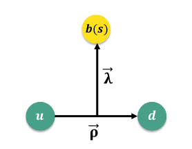
Figure 1: The definition of the internal Jacobi coordinates $\vec{\rho}$ and $\vec{\lambda}$, where we use green spheres to represent the $u$ and $d$ quarks and yellow spheres to represent the $b$ (or $s$) quark.

In this calculation, the Gaussian basis Hiyama:2003cu ; Yoshida:2015tia ; Yang:2019lsg ,

$$\begin{split}\phi_{nlm}^{G}(\vec{r})&=\phi^{G}_{nl}(r)~{}Y_{lm}(\hat{r})\\ &=\sqrt{\frac{2^{l+2}(2\nu_{n})^{l+3/2}}{\sqrt{\pi}(2l+1)!!}}\lim_{\varepsilon\to 0}\frac{1}{(\nu_{n}\varepsilon)^{l}}\sum_{k=1}^{k_{\text{max}}}C_{lm,k}e^{-\nu_{n}(\vec{r}-\varepsilon\vec{D}_{lm,k})^{2}},\end{split}$$ (4.15)

is used to expand the spatial wave functions $\phi_{\boldsymbol{l_{\rho}},\boldsymbol{ml_{\rho}}}$ and $\phi_{\boldsymbol{l_{\lambda}},\boldsymbol{ml_{\lambda}}}$ ($n=1,2,\cdots,n_{\text{max}}$), where the freedom parameter $n_{\text{max}}$ should be chosen from positive integers, and then the Gaussian size parameter $\nu_{n}$ can be settled as Luo:2022cun

$$\nu_{n}=1/r^{2}_{n},~{}~{}~{}r_{n}=r_{\text{min}}~{}a^{n-1},$$ (4.16)

where

$$a=\left(\frac{r_{\text{max}}}{r_{\text{min}}}\right)^{\frac{1}{n_{\text{max}}-1}}.$$

In our calculation the values of $\rho_{\text{min}}$ and $\rho_{\text{max}}$ are chosen to be $0.2$ fm and $2.0$ fm, respectively, and the parameter $n_{\rho_{\text{max}}}=6$. For the $\lambda$ mode, we also use the same Gaussian-sized parameters.

Table 2: Experimentally observed masses of charmed and bottom baryons used to fit the potential model parameters, where only the central values are given.

States	$J^{P}$	This work (GeV)	Expt. (GeV) ParticleDataGroup:2020ssz	States	$J^{P}$	This work (GeV)	Expt. (GeV) ParticleDataGroup:2020ssz
$\Lambda_{c}$	$\frac{1}{2}^{+}$	$2.286$	$2.286$	$\Lambda_{b}$	$\frac{1}{2}^{+}$	$5.621$	$5.619$
$\Lambda_{c}(2595)$	$\frac{1}{2}^{-}$	$2.595$	$2.595$	$\Lambda_{b}(5912)$	$\frac{1}{2}^{-}$	$5.896$	$5.912$
$\Lambda_{c}(2625)$	$\frac{3}{2}^{-}$	$2.627$	$2.625$	$\Lambda_{b}(5920)$	$\frac{3}{2}^{-}$	$5.909$	$5.919$
$\Lambda_{c}(2765)$	$?^{?}$	$2.768$	$2.765$	$\Lambda_{b}(6070)$	$\frac{1}{2}^{+}$	$6.046$	$6.072$
$\Lambda_{c}(2860)$	$\frac{3}{2}^{+}$	$2.872$	$2.856$	$\Lambda_{b}(6146)$	$\frac{3}{2}^{+}$	$6.133$	$6.146$
$\Lambda_{c}(2880)$	$\frac{5}{2}^{+}$	$2.894$	$2.881$	$\Lambda_{b}(6152)$	$\frac{5}{2}^{+}$	$6.144$	$6.152$
$\Sigma_{c}$	$\frac{1}{2}^{+}$	$2.446$	$2.453$	$\Sigma_{b}$	$\frac{1}{2}^{+}$	$5.809$	$5.811$
$\Sigma_{c}(2520)$	$\frac{3}{2}^{+}$	$2.519$	$2.518$	$\Sigma_{b}^{*}$	$\frac{3}{2}^{+}$	$5.835$	$5.832$
$\Xi_{c}$	$\frac{1}{2}^{+}$	$2.478$	$2.467$	$\Xi_{b}$	$\frac{1}{2}^{+}$	$5.809$	$5.794$
$\Xi_{c}(2790)$	$\frac{1}{2}^{-}$	$2.787$	$2.792$	$\Xi_{b}(6100)$	$\frac{3}{2}^{-}$	$6.093$	$6.100$
$\Xi_{c}(2815)$	$\frac{3}{2}^{-}$	$2.814$	$2.816$	$\Xi_{b}(6327)$ LHCb:2021ssn	$?^{?}$	$6.316$	$6.327$
$\Xi_{c}(2970)$	$?^{?}$	$2.953$	$2.970$	$\Xi_{b}(6333)$ LHCb:2021ssn	$?^{?}$	$6.324$	$6.332$
$\Xi_{c}(3055)$	$?^{?}$	$3.059$	$3.055$	$\Xi_{b}^{\prime}(5935)$	$\frac{1}{2}^{+}$	$5.939$	$5.935$
$\Xi_{c}(3080)$	$?^{?}$	$3.077$	$3.080$	$\Xi_{b}(5945)$	$\frac{3}{2}^{+}$	$5.963$	$5.949$
$\Xi_{c}^{\prime}$	$\frac{1}{2}^{+}$	$2.583$	$2.577$	$\Omega_{b}$	$\frac{1}{2}^{+}$	$6.043$	$6.046$
$\Xi_{c}(2645)$	$\frac{3}{2}^{+}$	$2.648$	$2.645$
$\Omega_{c}$	$\frac{1}{2}^{+}$	$2.693$	$2.695$
$\Omega_{c}(2770)$	$\frac{3}{2}^{+}$	$2.755$	$2.765$

Table 3: The comparison of the masses of $\Lambda_{b}$ and $\Lambda(1520)$ from our calculation and the PDG ParticleDataGroup:2020ssz data, and the radial components of the spatial wave functions of the concerned $\Lambda_{b}$ and $\Lambda(1520)$ from the semirelativistic potential model and GEM. The Gaussian bases $(n_{\rho},n_{\lambda})$ listed in the fourth column are arranged as $[(1,1),(1,2),\cdots,(1,n_{\lambda_{\text{max}}}),(2,1),(2,2),\cdots,(2,n_{\lambda_{\text{max}}}),\cdots,(n_{\rho_{\text{max}}},1),(n_{\rho_{\text{max}}},2),\cdots,(n_{\rho_{\text{max}}},n_{\lambda_{\text{max}}})]$.

States	This work (GeV)	Experiment (MeV) ParticleDataGroup:2020ssz	Eigenvectors
$\Lambda_{b}$	$5.621\pm 0.005$	$5619.60\pm 0.17$	$\big{[}0.0068\pm 0.0007,0.0442\pm 0.0014,0.0732\pm 0.0016,0.0032\pm 0.0003,$
			$0.0011\pm 0.0001,-0.0004\pm 0.0000,0.0270\pm 0.0012,0.0204\pm 0.0010,$
			$0.0273\pm 0.0022,0.0067\pm 0.0004,-0.0027\pm 0.0001,0.0007\pm 0.0000,$
			$-0.0170\pm 0.0002,0.2541\pm 0.0058,0.2427\pm 0.0006,0.0005\pm 0.0002,$
			$0.0060\pm 0.0001,-0.0017\pm 0.0000,-0.0037\pm 0.0003,-0.0426\pm 0.0010,$
			$0.4052\pm 0.0028,0.0253\pm 0.0025,-0.0023\pm 0.0007,0.0004\pm 0.0002,$
			$0.0071\pm 0.0001,-0.0052\pm 0.0008,0.0105\pm 0.0008,0.1224\pm 0.0015,$
			$-0.0246\pm 0.0001,0.0054\pm 0.0000,-0.0020\pm 0.0000,0.0010\pm 0.0003,$
			$-0.0112\pm 0.0003,-0.0139\pm 0.0001,0.0086\pm 0.0001,-0.0017\pm 0.0000\big{]}$
$\Lambda(1520)$	$1.561\pm 0.007$	$1517.5\pm 0.4$	$\big{[}0.0000\pm 0.0001,-0.0096\pm 0.0004,-0.0488\pm 0.0017,-0.0576\pm 0.0010$
			$-0.0011\pm 0.0001,-0.0004\pm 0.0000,-0.0049\pm 0.0004,0.0041\pm 0.0002$
			$-0.0295\pm 0.0012,-0.0279\pm 0.0020,0.0011\pm 0.0003,-0.0006\pm 0.0002$
			$-0.0010\pm 0.0001,-0.0510\pm 0.0019,-0.1771\pm 0.0036,-0.1890\pm 0.0014$
			$-0.0036\pm 0.0004,-0.0008\pm 0.0003,0.0003\pm 0.0001,0.0222\pm 0.0005$
			$-0.2146\pm 0.0003,-0.2766\pm 0.0040,-0.0001\pm 0.0013,-0.0036\pm 0.0006$
			$-0.0025\pm 0.0001,0.0028\pm 0.0001,0.0135\pm 0.0012,-0.1653\pm 0.0011$
			$-0.0174\pm 0.0008,0.0019\pm 0.0005,0.0010\pm 0.0000,-0.0020\pm 0.0000$
			$0.0035\pm 0.0004,0.0277\pm 0.0002,-0.0061\pm 0.0005,0.0010\pm 0.0003\big{]}$

In this paper, we fit the single charmed and bottom baryon spectrum to fix the phenomenological parameters in the semirelativistic potential model. The experimentally observed masses of charmed and bottom baryons are collected in Table 2. The $\chi^{2}$ method, i.e., finding the minimum $\chi^{2}$ value, is used for the fitting. In our fit, the $\chi^{2}$ value is defined as

$$\chi^{2}=\frac{1}{n(n-1)}\sum_{i}^{n}\Bigg{(}\frac{m_{i}^{\text{Exp}}-m_{i}^{\text{The}}}{\sigma_{i}}\Bigg{)}^{2},$$ (4.17)

where $m_{i}^{\text{Exp}}$ and $m_{i}^{\text{The}}$ are experimental and theoretical values of the mass of the $i$th baryon, respectively. The errors $\sigma_{i}=1\ \text{MeV}$ are universal for all baryons. In this fitting, the $\chi^{2}$ is given as 2.84. The fitted parameters are collected in Table 1. Meanwhile, our results for the masses of the charmed and bottom baryons are presented in Table 2.

With the above preparations, we can calculate the spatial wave functions of $\Lambda_{b}$ and $\Lambda(1520)$. Their masses and radial components of spatial wave functions are shown in Table 3. It is obvious that the calculated mass of $\Lambda_{b}$ is consistent with the Particle Data Group (PDG) ParticleDataGroup:2020ssz averaged value, while that of $\Lambda(1520)$ is about $40$ MeV higher than the PDG value.

V Numerical results

V.1 The weak transition form factors

With the input of the numerical wave functions of $\Lambda_{b}$ and $\Lambda^{\ast}$, and the complete expressions of the form factors obtained by solving Eq. (3.12) and Eqs. (LABEL:eq:ffs06)-(3.19), we present our numerical results of the form factors of the $\Lambda_{b}\to\Lambda^{\ast}$ transition. Since the form factors calculated in the light-front quark model are valid in the spacelike region ($q^{2}<0$), we have to extrapolate them to the timelike region ($q^{2}>0$).

Before we do the extrapolation, we need to talk about some constraints on the form factors at the $q^{2}=q^{2}_{\text{max}}$ point. To make sure that the helicity amplitudes in Eqs. (2.22)-(2.25) have no singularities and are nonzero values in the $q^{2}\to q^{2}_{\text{max}}$ limit, we get the constraints in this limit as

$$\begin{split}f_{t}^{V}=&O\Big{(}\frac{1}{\sqrt{s_{-}}}\Big{)},~{}f_{0}^{V}=O\Big{(}\frac{1}{s_{-}}\Big{)},~{}f_{\bot}^{V}=O\Big{(}\frac{1}{s_{-}}\Big{)},~{}f_{g}^{V}=O(1),\\ f_{t}^{A}=&O\Big{(}\frac{1}{s_{-}}\Big{)},~{}f_{0}^{A}=O\Big{(}\frac{1}{\sqrt{s_{-}}}\Big{)},~{}f_{\bot}^{A}=O\Big{(}\frac{1}{\sqrt{s_{-}}}\Big{)},~{}f_{g}^{A}=O\Big{(}\frac{1}{\sqrt{s_{-}}}\Big{)},\\ f_{0}^{T}=&O\Big{(}\frac{1}{s_{-}}\Big{)},~{}f_{\bot}^{T}=O\Big{(}\frac{1}{s_{-}}\Big{)},~{}f_{g}^{T}=O(1),\\ f_{0}^{T5}=&O\Big{(}\frac{1}{\sqrt{s_{-}}}\Big{)},~{}f_{\bot}^{T5}=O\Big{(}\frac{1}{\sqrt{s_{-}}}\Big{)},~{}f_{g}^{T5}=O\Big{(}\frac{1}{\sqrt{s_{-}}}\Big{)}.\end{split}$$ (5.1)

The form factors that show less singular behavior in the $q^{2}\to q^{2}_{\text{max}}$ limit are also reasonable. This would lead the helicity amplitudes to be zero in $q^{2}=q^{2}_{\text{max}}$. The above features have been discussed in Ref. Descotes-Genon:2019dbw . However, the above requirement is not strict enough, since it gives a broad limit. This will make nonunique extrapolations of the form factors.

Since the LQCD calculation of $\Lambda_{b}\to\Lambda(1520)$ form factors has been done in Refs. Meinel:2020owd ; Meinel:2021mdj , and their results work well in the kinematic region near $q_{\text{max}}^{2}$, we will talk about the characters of the form factors in the LQCD. The LQCD calculation has been completed in Refs. Meinel:2020owd ; Meinel:2021mdj . The authors obtained finite values of the form factors of $\Lambda_{b}\to\Lambda(1520)$ in their definition (i.e., $f_{0,+,\bot,\bot^{\prime}}$, $g_{0,+,\bot,\bot^{\prime}}$, $h_{+,\bot,\bot^{\prime}}$, and $\tilde{h}_{+,\bot,\bot^{\prime}}$) in the $q^{2}=q_{\text{max}}^{2}$ limit. Their definition of the form factors can be converted to ours by Meinel:2020owd

$$\begin{split}f_{t}^{V}=&\frac{m_{\Lambda^{*}}}{s_{+}}f_{0},~{}~{}f_{0}^{V}=\frac{m_{\Lambda^{*}}}{s_{-}}f_{+},~{}~{}~{}f_{\bot}^{V}=\frac{m_{\Lambda^{*}}}{s_{-}}f_{\bot},~{}~{}~{}f_{g}^{V}=f_{\bot^{\prime}},\\ f_{t}^{A}=&\frac{m_{\Lambda^{*}}}{s_{-}}g_{0},~{}~{}~{}f_{0}^{A}=\frac{m_{\Lambda^{*}}}{s_{+}}g_{+},~{}~{}~{}f_{\bot}^{A}=\frac{m_{\Lambda^{*}}}{s_{+}}g_{\bot},~{}~{}~{}f_{g}^{A}=-g_{\bot^{\prime}},\\ f_{0}^{T}=&\frac{m_{\Lambda^{*}}}{s_{-}}h_{+},~{}~{}~{}f_{\bot}^{T}=\frac{m_{\Lambda^{*}}}{s_{-}}h_{\bot},~{}~{}~{}f_{g}^{T}=(m_{\Lambda_{b}}+m_{\Lambda^{*}})h_{\bot^{\prime}},\\ f_{0}^{T5}=&\frac{m_{\Lambda^{*}}}{s_{+}}\tilde{h}_{+},~{}~{}~{}f_{\bot}^{T5}=\frac{m_{\Lambda^{*}}}{s_{+}}\tilde{h}_{\bot},~{}~{}~{}f_{g}^{T5}=-(m_{\Lambda_{b}}-m_{\Lambda^{*}})\tilde{h}_{\bot^{\prime}}.\end{split}$$ (5.2)

This shows that in the $q^{2}=q_{\text{max}}^{2}$ limit, the LQCD results Meinel:2021mdj show

$$\begin{split}f_{t}^{V}&=O(1),~{}~{}~{}f_{0}^{V}=O\Big{(}\frac{1}{s_{-}}\Big{)},~{}~{}~{}f_{\bot}^{V}=O\Big{(}\frac{1}{s_{-}}\Big{)},~{}~{}~{}f_{g}^{V}=O(1),\\ f_{0}^{A}&=O(1),~{}~{}~{}f_{\bot}^{A}=O(1),~{}~{}~{}f_{g}^{A}=O(1),\\ f_{0}^{T}&=O\Big{(}\frac{1}{s_{-}}\Big{)},~{}~{}~{}f_{\bot}^{T}=O\Big{(}\frac{1}{s_{-}}\Big{)},~{}~{}~{}f_{g}^{T}=O(1),\\ f_{0}^{T5}&=O(1),~{}~{}~{}f_{\bot}^{T5}=O(1),~{}~{}~{}f_{g}^{T5}=O(1).\end{split}$$ (5.3)

These characters fulfill the requirements. Also we have $g_{0}(q^{2})=\frac{a_{1}^{g_{0}}}{1-q^{2}/(m_{\text{pole}}^{f})^{2}}(\omega-1)$ Meinel:2021mdj with $\omega=(m_{\Lambda_{b}}^{2}+m_{\Lambda^{*}}^{2}-q^{2})/(2m_{\Lambda_{b}}m_{\Lambda^{*}})$, where $a_{1}^{g_{0}}$ is a nonzero value. According to Eq. (5.2), the $f_{t}^{A}(q^{2})=\frac{m_{\Lambda^{*}}}{s_{-}}\frac{a_{1}^{g_{0}}}{1-q^{2}/(m_{\text{pole}}^{f})^{2}}(\omega-1)$, and this implies, in the $q^{2}=q_{\text{max}}^{2}$ limit, that $f_{t}^{A}=O(1)$. This also satisfies the requirement.

In order to align with the LQCD results, we take the following strategy for the analytical continuation:

1. To do the extrapolations of the form factors $f_{t,g}^{V}$, $f_{t,0,\bot,g}^{A}$, $f_{g}^{T}$, and $f_{0,\bot,g}^{T5}$, the $z$-series form Boyd:1995cf ; Bourrely:2008za ; Khodjamirian:2011ub ; Amhis:2022vcd

   $$f(q^{2})=\frac{1}{1-q^{2}/(m_{\text{pole}}^{f})^{2}}\left[a_{0}^{f}+a_{1}^{f}z^{f}(q^{2})+a_{2}^{f}(z^{f}(q^{2}))^{2}\right]$$ (5.4)

   is adopted where $a_{0}^{f}$, $a_{1}^{f}$, and $a_{2}^{f}$ are free parameters needed to fit in the spacelike region, and

   $$\begin{split}z^{f}(q^{2})&=\frac{\sqrt{t_{+}^{f}-q^{2}}-\sqrt{t_{+}^{f}-t_{0}}}{\sqrt{t_{+}^{f}-q^{2}}+\sqrt{t_{+}^{f}-t_{0}}},\\ t_{\pm}^{f}&=(m_{B}\pm m_{K})^{2}.\end{split}$$ (5.5)

   The parameter $t_{0}$ is set to

   $$0\leqslant t_{0}=t_{+}\bigg{(}1-\sqrt{1-\frac{t_{-}}{t_{+}}}\bigg{)}\leqslant t_{-}.$$ (5.6)

   The $m^{f}_{\text{pole}}$ is collected in Table 4.

   Table 4: The pole masses of the form factors in Eq. (5.4), where the $0^{-}$, $1^{-}$, and $1^{+}$ masses are taken from the PDG ParticleDataGroup:2020ssz , while the $0^{+}$ mass is taken from the LQCD calculation Lang:2015hza .

   $f$	$J^{P}$	$m^{f}_{\text{pole}}(\text{GeV})$
   $f_{t}^{V}$	$0^{+}$	$5.711$
   $f_{g}^{V}$, $f_{g}^{T}$	$1^{-}$	$5.415$
   $f_{t}^{A}$	$0^{-}$	$5.367$
   $f_{0}^{A}$, $f_{\bot}^{A}$, $f_{g}^{A}$, $f_{0}^{T5}$, $f_{\bot}^{T5}$, $f_{g}^{T5}$	$1^{+}$	$5.828$

2. For the form factors $f_{0,\bot}^{V}$ and $f_{0,\bot}^{T}$, we use the form as

   $$f(q^{2})=\frac{1}{1-q^{2}/m_{-}^{2}}\left[a_{0}^{f}+a_{1}^{f}z^{f}(q^{2})+a_{2}^{f}(z^{f}(q^{2}))^{2}\right],$$ (5.7)

   where $m_{-}=m_{\Lambda_{b}}-m_{\Lambda^{*}}$.

To determine the parameters $a_{0}^{f}$, $a_{1}^{f}$, and $a_{2}^{f}$, we numerically calculate 24 points for each form factor by Eqs. (3.12)-(3.19) from $q^{2}=-q_{\text{max}}^{2}$ to $q^{2}=-0.01\ \text{GeV}^{2}$ in the spacelike region, and then fit them using Eq. (5.4) and Eq. (5.7) with the MINUIT program. The extrapolated parameters for the form factors of $\Lambda_{b}\to\Lambda^{\ast}$ are collected in Table 5. The $q^{2}$ dependence of the concerned form factors is shown in Fig. 2.

However, as discussed earlier, the less singular behaviors of $f_{0,\bot}^{V}$ and $f_{0,\bot}^{T}$ in the small-recoil limit are also not forbidden. Therefore, in this work, we also use the formula in Eq. (5.4) to perform the extrapolation of the form factors $f_{0,\bot}^{V}$ and $f_{0,\bot}^{T}$ again. This extrapolation scheme gives different results at the $q^{2}=q_{\text{max}}^{2}$ point for the four form factors, but has no effect on other form factors compared with the previous scheme. For clarification, we compare our results of the form factors in the $q^{2}=q_{\text{max}}^{2}$ point with the two different extrapolation schemes in Table 6. Finally, it should be emphasized that there is no established procedure for the extrapolation. The experimental measurement of $\Lambda_{b}\to\Lambda(1520)\ell^{+}\ell^{-}$ by the LHCb Collaboration can test the different extrapolation schemes.

Table 5: The form factors of the $\Lambda_{b}\to\Lambda^{\ast}$ transition in the standard light-front quark model.

Parameter	Value	Parameter	Value	Parameter	Value
$a_{0}^{f_{t}^{V}}$	$(0.1041\pm 0.0036)~{}\text{GeV}^{-1}$	$a_{1}^{f_{t}^{V}}$	$(-0.4493\pm 0.0375)~{}\text{GeV}^{-1}$	$a_{2}^{f_{t}^{V}}$	$(0.5425\pm 0.0954)~{}\text{GeV}^{-1}$
$a_{0}^{f_{0}^{V}}$	$(0.0850\pm 0.0037)~{}\text{GeV}^{-1}$	$a_{1}^{f_{0}^{V}}$	$(-0.2465\pm 0.0386)~{}\text{GeV}^{-1}$	$a_{2}^{f_{0}^{V}}$	$(0.0637\pm 0.0984)~{}\text{GeV}^{-1}$
$a_{0}^{f_{\bot}^{V}}$	$(0.1538\pm 0.0046)~{}\text{GeV}^{-1}$	$a_{1}^{f_{\bot}^{V}}$	$(-0.7505\pm 0.0478)~{}\text{GeV}^{-1}$	$a_{2}^{f_{\bot}^{V}}$	$(1.0292\pm 0.1210)~{}\text{GeV}^{-1}$
$a_{0}^{f_{g}^{V}}$	$0.0223\pm 0.0001$	$a_{1}^{f_{g}^{V}}$	$-0.0807\pm 0.0003$	$a_{2}^{f_{g}^{V}}$	$0.0798\pm 0.0031$
$a_{0}^{f_{t}^{A}}$	$(0.1052\pm 0.0026)~{}\text{GeV}^{-1}$	$a_{1}^{f_{t}^{A}}$	$(-0.5337\pm 0.0263)~{}\text{GeV}^{-1}$	$a_{2}^{f_{t}^{A}}$	$(0.7542\pm 0.0665)~{}\text{GeV}^{-1}$
$a_{0}^{f_{0}^{A}}$	$(0.0878\pm 0.0028)~{}\text{GeV}^{-1}$	$a_{1}^{f_{0}^{A}}$	$(-0.3647\pm 0.0293)~{}\text{GeV}^{-1}$	$a_{2}^{f_{0}^{A}}$	$(0.4197\pm 0.0747)~{}\text{GeV}^{-1}$
$a_{0}^{f_{\bot}^{A}}$	$(0.0804\pm 0.0022)~{}\text{GeV}^{-1}$	$a_{1}^{f_{\bot}^{A}}$	$(-0.3619\pm 0.0227)~{}\text{GeV}^{-1}$	$a_{2}^{f_{\bot}^{A}}$	$(0.4573\pm 0.0578)~{}\text{GeV}^{-1}$
$a_{0}^{f_{g}^{A}}$	$0.0441\pm 0.0023$	$a_{1}^{f_{g}^{A}}$	$-0.2012\pm 0.0240$	$a_{2}^{f_{g}^{A}}$	$0.2596\pm 0.0605$
$a_{0}^{f_{0}^{T}}$	$(-0.0178\pm 0.0003)~{}\text{GeV}^{-1}$	$a_{1}^{f_{0}^{T}}$	$(0.5398\pm 0.0037)~{}\text{GeV}^{-1}$	$a_{2}^{f_{0}^{T}}$	$(-1.4719\pm 0.0098)~{}\text{GeV}^{-1}$
$a_{0}^{f_{\bot}^{T}}$	$(0.0565\pm 0.0032)~{}\text{GeV}^{-1}$	$a_{1}^{f_{\bot}^{T}}$	$(-0.0233\pm 0.0331)~{}\text{GeV}^{-1}$	$a_{2}^{f_{\bot}^{T}}$	$(-0.3596\pm 0.0853)~{}\text{GeV}^{-1}$
$a_{0}^{f_{g}^{T}}$	$(0.0851\pm 0.0034)~{}\text{GeV}$	$a_{1}^{f_{g}^{T}}$	$(-0.4603\pm 0.0334)~{}\text{GeV}$	$a_{2}^{f_{g}^{T}}$	$(0.6616\pm 0.0805)~{}\text{GeV}$
$a_{0}^{f_{0}^{T5}}$	$(0.0923\pm 0.0026)~{}\text{GeV}^{-1}$	$a_{1}^{f_{0}^{T5}}$	$(-0.4516\pm 0.0272)~{}\text{GeV}^{-1}$	$a_{2}^{f_{0}^{T5}}$	$(0.6337\pm 0.0687)~{}\text{GeV}^{-1}$
$a_{0}^{f_{\bot}^{T5}}$	$(0.0790\pm 0.0020)~{}\text{GeV}^{-1}$	$a_{1}^{f_{\bot}^{T5}}$	$(-0.3482\pm 0.0206)~{}\text{GeV}^{-1}$	$a_{2}^{f_{\bot}^{T5}}$	$(0.4288\pm 0.0527)~{}\text{GeV}^{-1}$
$a_{0}^{f_{g}^{T5}}$	$(-0.3839\pm 0.0276)~{}\text{GeV}$	$a_{1}^{f_{g}^{T5}}$	$(1.6524\pm 0.2814)~{}\text{GeV}$	$a_{2}^{f_{g}^{T5}}$	$(-2.1223\pm 0.6945)~{}\text{GeV}$

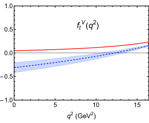
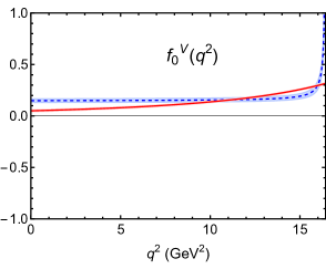
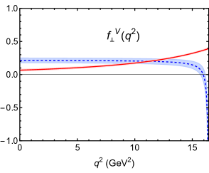
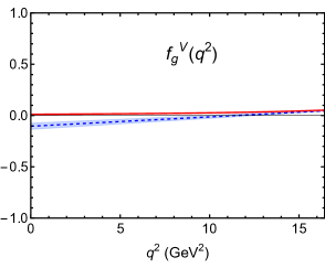
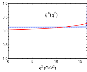
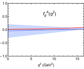
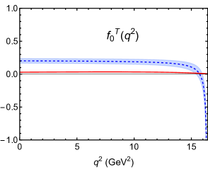
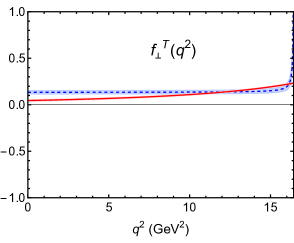
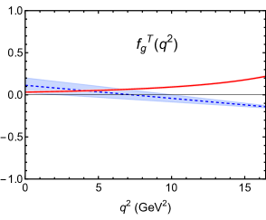
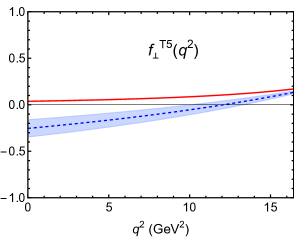
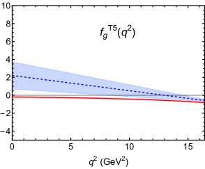
Figure 2: The $q^{2}$ dependence of the form factors of the vector, axial-vector, tensor, and pseudotensor type currents of the $\Lambda_{b}\to\Lambda^{\ast}$ transition, where the red solid curves are central values, and the light red bands are the corresponding errors. The units of the form factors are neglected here.

As shown in Eqs. (2.7)-(2.10), we need eight (axial-)vector and six (pseudo-)tensor form factors to describe the matrix elements in question. The number can apparently be reduced in the heavy quark limit $m_{b}\to\infty$. We speak separately of two different kinematic situations, i.e., the outgoing $\Lambda^{\ast}$ acts softly (the low-recoil limit) and acts energetically (the large-recoil limit). Accordingly, two effective theories, namely heavy quark effective theory (HQET) and soft-collinear effective theory (SCET), are developed to exploit the behaviors of the form factors.

In the low-recoil limit, where HQET is valid Isgur:1989vq ; Isgur:1990yhj ; Isgur:1990pm ; Mannel:1990vg , the weak transition matrix element can be re-expressed by two Isgur-Wise functions as Mannel:1990vg ; Das:2020cpv ; Bordone:2021bop

$$\langle\Lambda^{\ast}(p^{\prime})|\bar{s}\Gamma b|\Lambda_{b}(p)\rangle=\bar{u}_{\Lambda}^{\alpha}(p^{\prime})\upsilon_{\alpha}\left[\zeta_{1}(\omega)+\not{\upsilon}\zeta_{2}(\omega)\right]\Gamma u_{\Lambda_{b}}(p).$$ (5.8)

Here, $\Gamma$ is an arbitrary Dirac structure, and $\omega=\upsilon\cdot\upsilon^{\prime}=(m_{\Lambda_{b}}^{2}+m_{\Lambda^{\ast}}^{2}-q^{2})/(2m_{\Lambda_{b}}m_{\Lambda^{\ast}})$, where $\upsilon=p/m_{\Lambda_{b}}$ and $\upsilon^{\prime}=p^{\prime}/m_{\Lambda^{\ast}}$ represent the four velocities of the bottom baryon and hyperon, respectively. The eight form factors are derived as two independent form factors $\zeta_{1}(\omega)$ and $\zeta_{2}(\omega)$. In the low-recoil limit this gives $q^{2}\to q_{\text{max}}^{2}\equiv(m_{\Lambda_{b}}-m_{\Lambda^{\ast}})^{2}$ (or $\omega\to 1$). With slightly different definitions of the form factors in Refs. Boer:2014kda ; Feldmann:2011xf ; Mannel:2011xg ,we have Descotes-Genon:2019dbw

$$\begin{split}f_{t}^{V}(q_{\text{max}}^{2})&\simeq f_{0}^{A}(q_{\text{max}}^{2})\simeq f_{\bot}^{A}(q_{\text{max}}^{2})\\ &\simeq f_{0}^{T5}(q_{\text{max}}^{2})\simeq f_{\bot}^{T5}(q_{\text{max}}^{2})\simeq\big{[}\zeta_{1}(1)+\zeta_{2}(1)\big{]}/m_{\Lambda_{b}},\\ f_{0}^{V}(q_{\text{max}}^{2})&\simeq f_{t}^{A}(q_{\text{max}}^{2})\simeq f_{\bot}^{V}(q_{\text{max}}^{2})\\ &\simeq f_{0}^{T}(q_{\text{max}}^{2})\simeq f_{\bot}^{T}(q_{\text{max}}^{2})\simeq\big{[}\zeta_{1}(1)-\zeta_{2}(1)\big{]}/m_{\Lambda_{b}},\\ f_{g}^{V}(q_{\text{max}}^{2})&\simeq f_{g}^{A}(q_{\text{max}}^{2})\simeq f_{g}^{T}(q_{\text{max}}^{2})\simeq f_{g}^{T5}(q_{\text{max}}^{2})\simeq 0,\end{split}$$ (5.9)

while in the large-recoil limit where SCET is valid, we have Mannel:2011xg ; Feldmann:2011xf ; Wang:2011uv

$$\langle\Lambda^{\ast}(p^{\prime})|\bar{s}\Gamma b|\Lambda_{b}(p)\rangle=\bar{u}_{\Lambda}^{\alpha}(p^{\prime})\upsilon_{\alpha}\left[\zeta(\omega)\right]\Gamma u_{\Lambda_{b}}(p),$$ (5.10)

where $\zeta(\omega)$ is the only remaining form factor. This gives, in the large-recoil limit, $q^{2}\to 0$ (or $\omega\to(m_{\Lambda_{b}}^{2}+m_{\Lambda^{\ast}}^{2})/(2m_{\Lambda_{b}}m_{\Lambda^{\ast}})$),

$$\begin{split}f_{t}^{V}(0)&\simeq f_{0}^{V}(0)\simeq f_{\bot}^{V}(0)\simeq f_{t}^{A}(0)\simeq f_{0}^{A}(0)\simeq f_{\bot}^{A}(0)\\ &\simeq f_{0}^{T}(0)\simeq f_{\bot}^{T}(0)\simeq f_{0}^{T5}(0)\simeq f_{\bot}^{T5}(0)\\ &\simeq\zeta\big{(}\frac{m_{\Lambda_{b}}^{2}+m_{\Lambda^{\ast}}^{2}}{2m_{\Lambda_{b}}m_{\Lambda^{\ast}}}\big{)}\big{/}m_{\Lambda_{b}},\end{split}$$ (5.11)

and four $f_{g}$ form factors will disappear. From Fig. 2, we can see that apart from the $f_{g}^{T(T5)}(q^{2})$, which deviates from the predictions, the remaining calculated form factors are consistent with the requirements of HQET and SCET.

In addition, Bordone has completed the heavy quark expansion (HQE) calculation of the $\Lambda_{b}\to\Lambda^{*}$ form factors beyond the leading order Bordone:2021bop . At the zero-recoil limit, the HQE predicts the ratios of the form factors, which are independent of the Isgur-Wise functions, as Bordone:2021bop

$$\begin{split}\frac{F_{1/2,0}}{F_{1/2,\bot}}=&\frac{F_{1/2,0}}{F_{3/2,\bot}}=-2\frac{m_{\Lambda_{b}}-m_{\Lambda^{*}}}{m_{\Lambda_{b}}+m_{\Lambda^{*}}}=-1.15,\\ \frac{F_{1/2,\bot}}{F_{3/2,\bot}}=&1,~{}~{}\frac{T_{1/2,0}}{T_{1/2,\bot}}=-2\frac{m_{\Lambda_{b}}+m_{\Lambda^{*}}}{m_{\Lambda_{b}}-m_{\Lambda^{*}}}=-3.48,\\ \frac{T_{1/2,0}}{T_{3/2,\bot}}=&\frac{2m_{\Lambda^{*}}}{m_{\Lambda_{b}}-m_{\Lambda^{*}}}=0.74,~{}~{}\frac{T_{1/2,\bot}}{T_{3/2,\bot}}=-\frac{m_{\Lambda^{*}}}{m_{\Lambda_{b}}+m_{\Lambda^{*}}}=-0.21.\end{split}$$ (5.12)

Note that the form factor base used in Ref. Bordone:2021bop is different from ours. By using the conversions collected in Appendix B of Ref. Bordone:2021bop and Eq. (5.2), we can get our results of these ratios as:

$$\begin{split}\frac{F_{1/2,0}^{\small{\text{this~{}work}}}}{F_{1/2,\bot}^{\small{\text{this~{}work}}}}=&\frac{f_{0}^{V}}{f_{\bot}^{V}}=0.521\pm 0.026,\\ \frac{F_{1/2,\bot}^{\small{\text{this~{}work}}}}{F_{3/2,\bot}^{\small{\text{this~{}work}}}}=&-\frac{s_{-}}{m_{\Lambda^{*}}}\frac{f_{\bot}^{V}}{f_{g}^{V}}=-33.8\pm 0.9,\\ \frac{F_{1/2,0}^{\small{\text{this~{}work}}}}{F_{3/2,\bot}^{\small{\text{this~{}work}}}}=&-\frac{s_{-}}{m_{\Lambda^{*}}}\frac{f_{0}^{V}}{f_{g}^{V}}=-17.6\pm 0.7,\\ \frac{T_{1/2,0}^{\small{\text{this~{}work}}}}{T_{1/2,\bot}^{\small{\text{this~{}work}}}}=&\frac{f_{0}^{T}}{f_{\bot}^{T}}=-0.63\pm 0.04,\\ \frac{T_{1/2,0}^{\small{\text{this~{}work}}}}{T_{3/2,\bot}^{\small{\text{this~{}work}}}}=&s_{-}\frac{f_{0}^{T}}{f_{g}^{T}}=-2.56\pm 0.09,\\ \frac{T_{1/2,\bot}^{\small{\text{this~{}work}}}}{T_{3/2,\bot}^{\small{\text{this~{}work}}}}=&s_{-}\frac{f_{\bot}^{T}}{f_{g}^{T}}=4.09\pm 0.28.\end{split}$$ (5.13)

Our results are very different from those of the HQE.

In addition, we also compare our results of the form factors with the NRQM Mott:2015zma and the LQCD Meinel:2021mdj at $q^{2}=0$ and $q^{2}=q_{\text{max}}^{2}$ endpoints in Table 6. Until now, less work has been done on the $\Lambda_{b}\to\Lambda(1520)$ transition, so more theoretical work is needed to validate these form factors.

Table 6: Theoretical predictions for the form factors of $\Lambda_{b}\to\Lambda(1520)$ at the endpoints of $q^{2}=0$ and $q^{2}=q_{\text{max}}^{2}$ using different approaches.

	This work	NRQM Mott:2015zma	LQCD Meinel:2021mdj		$\text{This\ work}^{[a]}$	$\text{This\ work}^{[b]}$	NRQM Mott:2015zma	LQCD Meinel:2021mdj
$f_{t}^{V}(0)$	$0.051\pm 0.007$	$0.0029$	$-0.1523\pm 0.0530$	$f_{t}^{V}(q_{\text{max}}^{2})$	$0.244\pm 0.008$	$0.244\pm 0.008$	$\infty$	$0.1726\pm 0.0138$
$f_{0}^{V}(0)$	$0.051\pm 0.007$	$0.0029$	$0.0714\pm 0.0078$	$f_{0}^{V}(q_{\text{max}}^{2})$	$\infty$	$0.336\pm 0.008$	$\infty$	$\infty$
$f_{\bot}^{V}(0)$	$0.067\pm 0.009$	$0.0042$	$0.1093\pm 0.0151$	$f_{\bot}^{V}(q_{\text{max}}^{2})$	$\infty$	$0.416\pm 0.011$	$\infty$	$\infty$
$f_{g}^{V}(0)$	$0.0123\pm 0.0001$	$-0.0002$	$-0.0385\pm 0.0138$	$f_{g}^{V}(q_{\text{max}}^{2})$	$0.0582\pm 0.0002$	$0.0582\pm 0.0002$	$0.0323$	$0.0481\pm 0.0028$
$f_{t}^{A}(0)$	$0.044\pm 0.005$	$0.0031$	$0.0705\pm 0.0060$	$f_{t}^{A}(q_{\text{max}}^{2})$	$0.293\pm 0.006$	$0.293\pm 0.006$	$\infty$	$0.1695\pm 0.0145$
$f_{0}^{A}(0)$	$0.044\pm 0.005$	$0.0031$	$-0.1283\pm 0.0471$	$f_{0}^{A}(q_{\text{max}}^{2})$	$0.197\pm 0.006$	$0.197\pm 0.006$	$0.1791$	$0.1449\pm 0.0109$
$f_{\bot}^{A}(0)$	$0.038\pm 0.004$	$0.0033$	$-0.1260\pm 0.0471$	$f_{\bot}^{A}(q_{\text{max}}^{2})$	$0.182\pm 0.005$	$0.182\pm 0.005$	$0.1637$	$0.1430\pm 0.0109$
$f_{g}^{A}(0)$	$0.020\pm 0.004$	$0.0004$	$0.0086\pm 0.0830$	$f_{g}^{A}(q_{\text{max}}^{2})$	$0.100\pm 0.005$	$0.100\pm 0.005$	$0.0532$	$0.0415\pm 0.0145$
$f_{0}^{T}(0)$	$0.0294\pm 0.0007$	$0.0038$	$0.0986\pm 0.0151$	$f_{0}^{T}(q_{\text{max}}^{2})$	$\infty$	$0.0026\pm 0.0021$	$\infty$	$\infty$
$f_{\bot}^{T}(0)$	$0.046\pm 0.006$	$0.0030$	$0.0690\pm 0.0077$	$f_{\bot}^{T}(q_{\text{max}}^{2})$	$\infty$	$0.246\pm 0.007$	$\infty$	$\infty$
$f_{g}^{T}(0)$	$0.032\pm 0.006$	$-0.0041$	$0.0130\pm 0.0376$	$f_{g}^{T}(q_{\text{max}}^{2})$	$0.234\pm 0.008$	$0.234\pm 0.008$	$-0.1509$	$-0.1506\pm 0.0127$
$f_{0}^{T5}(0)$	$0.040\pm 0.005$	$0.0032$	$-0.1207\pm 0.0500$	$f_{0}^{T5}(q_{\text{max}}^{2})$	$0.211\pm 0.005$	$0.211\pm 0.005$	$0.1861$	$0.1412\pm 0.0127$
$f_{\bot}^{T5}(0)$	$0.038\pm 0.004$	$0.0030$	$-0.1333\pm 0.0471$	$f_{\bot}^{T5}(q_{\text{max}}^{2})$	$0.178\pm 0.004$	$0.178\pm 0.004$	$0.1897$	$0.1476\pm 0.0127$
$f_{g}^{T5}(0)$	$-0.19\pm 0.05$	$0.0072$	$1.167\pm 0.688$	$f_{g}^{T5}(q_{\text{max}}^{2})$	$-0.86\pm 0.06$	$-0.86\pm 0.06$	$-0.3268$	$-0.5826\pm 0.0918$

• These results, listed in the fourth column, are obtained by the first extrapolation scheme. Here, the $f_{t,g}^{V}$, $f_{t,0,\bot,g}^{A}$, $f_{g}^{T}$ and $f_{0,\bot,g}^{T5}$ are extrapolated by Eq. (5.4), while the $f_{0,\bot}^{V}$ and $f_{0,\bot}^{T}$ are extrapolated by Eq. (5.7).

• These results, shown in the fifth column, are from the second extrapolation scheme. Here, all form factors are extrapolated by Eq. (5.4).

V.2 The branching ratio and angular observables

With the above preparations, we will present our numerical results. The baryon and lepton masses used in our calculation are taken from the PDG ParticleDataGroup:2020ssz , as well as $\tau_{\Lambda_{b}}=1.470$ ps. We also use $\mathcal{B}_{\Lambda^{\ast}}\equiv\mathcal{B}\big{(}\Lambda^{\ast}\to N\bar{K}\big{)}=45\%$ ParticleDataGroup:2020ssz . To compare with the experimental data, we examine a number of angular observables, including the $CP$-averaged normalized angular coefficients, the differential branching ratios, the lepton’s forward-backward asymmetry $(A_{FB}^{\ell})$, and the transverse ($F_{T}$) and longitudinal ($F_{L}$) polarization fractions of the dilepton system.

First, we examine the $CP$-averaged normalized angular distributions

$$S_{i}=\frac{L_{i}+\bar{L}_{i}}{d(\Gamma+\bar{\Gamma})/dq^{2}},$$ (5.14)

where the angular distributions $L_{i}$ and the differential decay width $d\Gamma/dq^{2}$ are defined in Eqs. (2.34) and (2.35), respectively. For the $CP$-conjugated mode, the corresponding expression for the angular decay distribution should be written as

$$\frac{d^{4}\bar{\Gamma}}{dq^{2}d\cos\theta_{\Lambda^{\ast}}d\cos\theta_{\ell}d\phi}=\frac{3}{8\pi}\sum_{i}\bar{L}_{i}(q^{2})f_{i}(q^{2},\theta_{\ell},\theta_{\Lambda^{*}},\phi),$$ (5.15)

where $\bar{L}_{i}(q^{2})$ can be obtained by doing the full conjugation for all weak phases in $L_{i}(q^{2})$. We should also do the substitutions as

$$\begin{split}L_{1c,2c}&\to-\bar{L}_{1c,2c},~{}~{}L_{1cc,1ss,2cc,2ss}\to\bar{L}_{1cc,1ss,2cc,2ss},\\ L_{3ss}&\to\bar{L}_{3ss},~{}~{}~{}L_{4ss}\to-\bar{L}_{4ss},\\ L_{5s}&\to-\bar{L}_{5s},~{}~{}~{}L_{5sc}\to\bar{L}_{5sc},\\ L_{6s}&\to\bar{L}_{6s},~{}~{}~{}L_{6sc}\to-\bar{L}_{6sc},\end{split}$$ (5.16)

where the minus sign is a result from the operations of $\theta_{\ell}\to\theta_{\ell}-\pi$ and $\phi\to-\phi$. The differential decay width of the conjugated mode is

$$\frac{d\bar{\Gamma}}{dq^{2}}=\frac{1}{3}(\bar{L}_{1cc}+2\bar{L}_{1ss}+2\bar{L}_{2cc}+4\bar{L}_{2ss}+2\bar{L}_{3ss}).$$ (5.17)

In Fig. 3, we present our results for the $q^{2}$ dependent normalized angular coefficients. Since the $e$ channel shows similar behavior to the $\mu$ channel, we only present the results of the $\mu$ and the $\tau$ channels here. These angular distributions are important physical observables, and can be checked by future experiments.

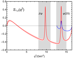
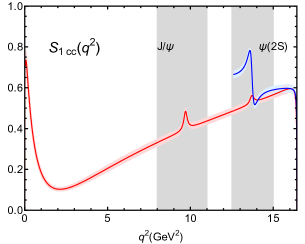
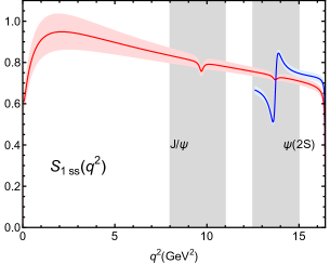
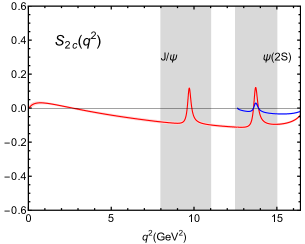
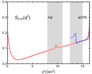
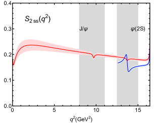
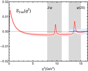
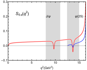
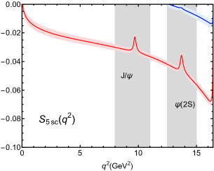
Figure 3: The $q^{2}$ dependence of the normalized angular coefficients $S_{1c}$, $S_{1cc}$, $S_{1ss}$, $S_{2c}$, $S_{2cc}$, $S_{2ss}$, $S_{3ss}$, $S_{5s}$, and $S_{5sc}$. Here, the red curve and the blue curve are our results of the $\mu$ and $\tau$ channels, respectively, and the concomitant shadows are corresponding errors.

At the low-recoil endpoint for $q^{2}\to(m_{\Lambda_{b}}-m_{\Lambda^{*}})^{2}$, Descotes-Genon and Novoa-Brunet predicted Descotes-Genon:2019dbw

$$\begin{split}S_{1c}&\to 0,~{}~{}S_{2cc}-S_{1cc}/4\to 3/8,\\ S_{3ss}&\to-1/4,~{}~{}S_{5sc}\to-1/2\end{split}$$

by neglecting the contribution from the photon pole. In Fig. 4, we present the behavior of the normalized angular coefficients $S_{1c}$, $S_{2cc}-S_{1cc}/4$, $S_{3ss}$, and $S_{5sc}$ in the low-recoil region by assuming $m_{\ell}=0$. It is obvious that our result for $S_{1c}$ is strictly consistent with the above prediction, while the $S_{2cc}-S_{1cc}/4$, $S_{3ss}$ and $S_{5sc}$ show apparent deviations.

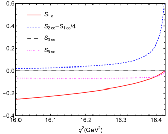
Figure 4: The behaviors of the normalized angular coefficients $S_{1c}$, $S_{2cc}-S_{1cc}/4$, $S_{3ss}$, and $S_{5sc}$ in the low-recoil region with $m_{\ell}=0$.

We further evaluate the differential branching ratios using Eq. (2.35). The $q^{2}$ dependence of the differential branching ratios is shown in Fig. 5, where the orange solid curve, the blue dashed curve, and the purple dot-dashed curve are our results for the $e$, $\mu$, and $\tau$ channels, respectively. The gray zones in the regions of the dilepton mass squared $8.0<q^{2}<11.0\ \text{GeV}^{2}$ and $12.5<q^{2}<15.0\ \text{GeV}^{2}$ show the contributions from the charmonium resonances $J/\psi$ and $\psi(2S)$, respectively.

Recently, the LHCb collaboration measured the “nonresonant” contributions, which are different from the “resonant” contribution from $\Lambda_{b}^{0}\to pK^{-}J\psi(\to\ell^{+}\ell^{-})$, to $\mathcal{B}(\Lambda_{b}^{0}\to pK^{-}e^{+}e^{-})$ and $\mathcal{B}(\Lambda_{b}^{0}\to pK^{-}\mu^{+}\mu^{-})$ decays as

$$\mathcal{B}(\Lambda_{b}^{0}\!\to\!pK^{-}e^{+}e^{-})\! \!=\! \!(3.1\!\pm 0.4\!\pm 0.2\!\pm 0.3^{+0.4}_{-0.3})\times 10^{-7},$$

$$\mathcal{B}(\Lambda_{b}^{0}\!\to\!pK^{-}\mu^{+}\mu^{-})\! \!=\! \!(2.65\!\pm 0.14\!\pm 0.12\!\pm 0.29^{+0.38}_{-0.23})\times 10^{-7},$$

in the region of $0.1\leq q^{2}\leq 6$ $\text{GeV}^{2}/c^{4}$ and $m(pK^{-})<2600\ \text{MeV}/c^{2}$ LHCb:2019efc . Assuming $\mathcal{B}(\Lambda(1520)\to pK^{-})=\mathcal{B}(\Lambda(1520)\to n\bar{K}^{0})$, we calculate

$$\mathcal{B}(\Lambda_{b}^{0}\to\Lambda^{\ast}(\to pK^{-})e^{+}e^{-})_{0.1\leq q^{2}\leq 6\ \text{GeV}^{2}}$$

$$=(1.618\pm 0.108)\times 10^{-7},$$

$$\mathcal{B}(\Lambda_{b}^{0}\to\Lambda^{\ast}(\to pK^{-})\mu^{+}\mu^{-})_{0.1\leq q^{2}\leq 6\ \text{GeV}^{2}}$$

$$=(1.610\pm 0.106)\times 10^{-7}.$$

This indicates that the contribution from $\Lambda(1520)$ is significant. We find from the PDG ParticleDataGroup:2020ssz that $\Lambda(1600)$, $\Lambda(1670)$, and other hyperons can also decay to the $N\bar{K}$ final state. Their contributions need to be carefully studied. Further studies with more excited $\Lambda$ hyperons will make a difference to the $\Lambda_{b}^{0}\to pK^{-}\ell^{+}\ell^{-}$ decays.

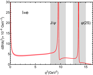
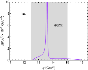
Figure 5: The $q^{2}$ dependence of the differential branching ratios for $\Lambda_{b}\to\Lambda^{\ast}(\to N\bar{K})\ell^{+}\ell^{-}$ ($\ell=e~{}(\text{left~{}panel})$, $\mu~{}(\text{center~{}panel})$, $\tau~{}(\text{right~{}panel})$), where the red, the blue, and the purple curves are our results from the $e$, $\mu$, and $\tau$ channels, respectively, and the concomitant shadows are the corresponding errors.

In addition, the $q^{2}$ dependence of the lepton-side forward-backward asymmetry $(A_{FB}^{\ell})$, and the transverse ($F_{T}$) and longitudinal ($F_{L}$) polarization fractions of the dilepton system are presented in Figs. 6, 7 and 8, respectively, where we also show the contributions from the charmonium resonances $J/\psi$ and $\psi(2S)$ with gray zones. The averaged values of these angular observables for the $e$ and $\mu$ channels defined in Eq. (2.39) in the region of $0.1<q^{2}<6.0\ \text{GeV}^{2}$ are presented in Table 7. The angular distributions provide a rich set of physical observables to study the weak interaction and the structure of $\Lambda(1520)$, and are also important to study the NP effects beyond the SM Azizi:2012vy ; Yan:2019tgn ; Descotes-Genon:2019dbw ; Das:2020cpv ; Amhis:2020phx , so we call for the ongoing LHCb experiment to measure them.

Table 7: The predictions for the averaged lepton-side forward-backward asymmetry $\langle A_{FB}^{\ell}\rangle$, the averaged transverse polarization fraction $\langle F_{T}\rangle$, and the averaged longitudinal polarization fraction $\langle F_{L}\rangle$ in the region of $0.1<q^{2}<6.0\ \text{GeV}^{2}$.

Channels	$\langle A_{FB}^{\ell}\rangle$	$\langle F_{T}\rangle$	$\langle F_{L}\rangle$
$\ell=e$	$-0.030\pm 0.012$	$0.208\pm 0.055$	$0.792\pm 0.231$
$\ell=\mu$	$-0.032\pm 0.010$	$0.221\pm 0.057$	$0.779\pm 0.225$

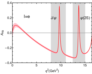
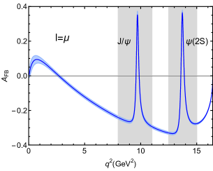
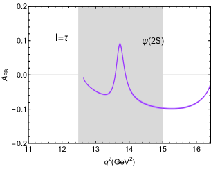
Figure 6: The $q^{2}$ dependence of the lepton-side forward-backward asymmetry parameter $(A_{FB}^{\ell})$ for $\Lambda_{b}\to\Lambda^{*}(\to N\bar{K})\ell^{+}\ell^{-}$ ($\ell=e~{}(\text{left~{}panel})$, $\mu~{}(\text{center~{}panel})$, $\tau~{}(\text{right~{}panel})$), where the red, blue, and purple curves are our results from the $e$, $\mu$, and $\tau$ channels, respectively, and the shadows are the corresponding errors.

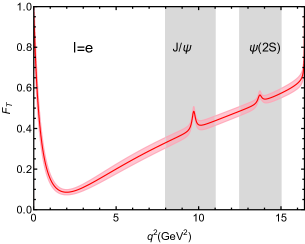
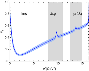
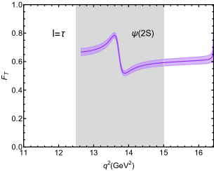
Figure 7: The $q^{2}$ dependence of the transverse polarization fractions ($F_{T}$) for $\Lambda_{b}\to\Lambda^{*}(\to N\bar{K})\ell^{+}\ell^{-}$ ($\ell=e~{}(\text{left~{}panel})$, $\mu~{}(\text{center~{}panel})$, $\tau~{}(\text{right~{}panel})$), where the red, blue, and purple curves are our results of the $e$, $\mu$, and $\tau$ channels, respectively, and the shadows are the corresponding errors.

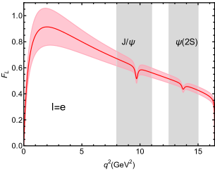
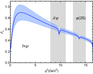
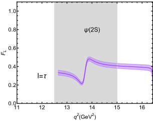
Figure 8: The $q^{2}$ dependence of the longitudinal polarization fractions ($F_{L}$) for $\Lambda_{b}\to\Lambda^{*}(\to N\bar{K})\ell^{+}\ell^{-}$ ($\ell=e~{}(\text{left~{}panel})$, $\mu~{}(\text{center~{}panel})$, $\tau~{}(\text{right~{}panel})$), where the red, blue, and purple curves are our results of the $e$, $\mu$, and $\tau$ channels, respectively, and the shadows are the corresponding errors.

VI Summary

With the accumulation of experimental data in the LHCb Collaboration, the experimental exploration of rare decays $b\to s\ell^{+}\ell^{-}$ ($\ell$=$e$, $\mu$, $\tau$) in the baryon sector, especially the $P$-wave final state $\Lambda_{b}\to\Lambda(1520)\ell^{+}\ell^{-}$, will attract more attention. Given this opportunity, in this work we focus on the quasi-four-body decay $\Lambda_{b}\to\Lambda(1520)(\to N\bar{K})\ell^{+}\ell^{-}$, where the angular coefficients, the differential branching ratio, and several angular observables, including the lepton-side forward-backward asymmetry $(A_{FB}^{\ell})$, and the transverse and longitudinal polarization fractions $(F_{T(L)})$ are investigated.

To describe the weak process, we have worked in the helicity formula, where the relevant weak transition form factors are obtained through the three-body light-front quark model. Our main advantage is the improved treatment of the spatial wave functions of the involved baryons, where a semirelativistic potential model is applied to solve the numerical spatial wave functions of the baryons assisted by the GEM. Thus, we emphasize that our study of the rare decay $\Lambda_{b}\to\Lambda(1520)(\to N\bar{K})\ell^{+}\ell^{-}$ is supported by the baryon spectroscopy. Our results of the form factors are comparable with the predictions of HQET and SCET, and also with the calculations by the LQCD approach. These form factors will be useful for the study of the corresponding weak decays.

Overall, we have systematically investigated the $\Lambda_{b}\to\Lambda(1520)(\to N\bar{K})\ell^{+}\ell^{-}$ ($\ell=e,\mu,\tau$) processes in the framework of the three-body light-front quark model based on the Gaussian expansion method. We believe that the present work can serve as an essential step toward strong dynamics on the beauty baryon decays. We expect that under the considerable progress on the experimental side, the above predictions could be tested by future LHCb experiments.

Appendix A The differential decay width

The differential decay width for the quasi-four-body decay $\Lambda_{b}\to\Lambda^{*}(\to N\bar{K})\ell^{+}\ell^{-}$ is

$$d\Gamma=\frac{|\mathcal{M}|^{2}}{2m_{\Lambda_{b}}}d\Phi_{4}(p;k_{1},k_{2},q_{1},q_{2}),$$ (A.1)

where $d\Phi_{4}$ is the four-body phase space given by

$$\begin{split}d\Phi_{4}&(p;k_{1},k_{2},q_{1},q_{2})\\ =&(2\pi)^{4}\delta^{4}\Big{(}p\!-\!k_{1}\!-\!k_{2}\!-q_{1}\!-\!q_{2}\Big{)}\prod_{i=1}^{2}\!\frac{d^{3}\vec{k}_{i}}{(2\pi)^{3}2E_{k_{i}}}\prod_{j=1}^{2}\!\frac{d^{3}\vec{q}_{j}}{(2\pi)^{3}2E_{q_{j}}}\\ =&\frac{dk^{2}}{2\pi}\frac{dq^{2}}{2\pi}d\Phi_{2}(k;k_{1},k_{2})d\Phi_{2}(q;q_{1},q_{2})d\Phi_{2}(p;k,q),\end{split}$$ (A.2)

where the two-body phase spaces are written as

$$\begin{split}\int\!d\Phi_{2}(k;k_{1},k_{2})\!=&\frac{1}{32\pi^{2}}\frac{\sqrt{\lambda(k^{2},k_{1}^{2},k_{2}^{2})}}{k^{2}}\!\int_{-1}^{1}\!d\cos\theta_{\Lambda^{\ast}}\!\int_{0}^{2\pi}\!d\phi,\\ \int\!d\Phi_{2}(q;q_{1},q_{2})\!=&\frac{1}{32\pi^{2}}\frac{\sqrt{\lambda(q^{2},q_{1}^{2},q_{2}^{2})}}{q^{2}}\!\int_{-1}^{1}\!d\cos\theta_{\ell}\times(2\pi),\\ \int\!d\Phi_{2}(p;k,q)\!=&\frac{1}{32\pi^{2}}\frac{\sqrt{\lambda(p^{2},k^{2},q^{2})}}{p^{2}}\times 2\times(2\pi).\end{split}$$ (A.3)

As shown in Fig. 9, three angles are defined (i) the angle $\theta_{\Lambda^{\ast}}$ is defined as the angle that the nucleon makes with the $+z$ axis in the $(N\bar{K})$ center of mass system, (ii) the angle $\theta_{\ell}$ is defined as the angle made by the $\ell^{-}$ with the $+z$ axis in the $(\ell^{+}\ell^{-})$ cms, and (iii) the angle $\phi$ between the two decay planes, respectively.

The decay width of the concerned decay $\Lambda_{b}\to\Lambda^{\ast}(\to N\bar{K})\ell^{+}\ell^{-}$ is expressed as

$$\begin{split}\int\!d\Phi_{4}\frac{|\mathcal{M}|^{2}}{2m_{\Lambda_{b}}}\!=&\frac{2}{(32\pi^{2})^{3}}\!\int\!dk^{2}\frac{\sqrt{\lambda(k^{2},k_{1}^{2},k_{2}^{2})}}{k^{2}}\frac{\sqrt{\lambda(q^{2},q_{1}^{2},q_{2}^{2})}}{q^{2}}\\ &\times\frac{\sqrt{\lambda(p^{2},k^{2},q^{2})}}{p^{2}}(dq^{2}d\cos\theta_{\Lambda^{\ast}}d\cos\theta_{\ell}d\phi)\\ &\times\frac{|\mathcal{M}|^{2}}{2m_{\Lambda_{b}}}.\end{split}$$ (A.4)

We also take into account the width of $\Lambda^{\ast}$ to modify its propagator, but treat it as narrow ($\Gamma_{\Lambda^{\ast}}\ll m_{\Lambda^{\ast}}$) state. This gives Yan:2019tgn ,

$$\begin{split}\int\!d\Phi_{4}\frac{|\mathcal{M}|^{2}}{2m_{\Lambda_{b}}}=&\int\!d\Phi_{4}\frac{|\mathcal{M}|^{2}}{2m_{\Lambda_{b}}}\frac{1}{(k^{2}-m_{\Lambda^{\ast}}^{2})^{2}}(k^{2}-m_{\Lambda^{\ast}}^{2})^{2}\\ \stackrel{{\scriptstyle\Gamma_{\Lambda^{\ast}}\ll m_{\Lambda^{\ast}}}}{{\longrightarrow}}&\int\!d\Phi_{4}\frac{|\mathcal{M}|^{2}}{2m_{\Lambda_{b}}}\frac{(k^{2}-m_{\Lambda^{\ast}}^{2})^{2}}{(k^{2}-m_{\Lambda^{\ast}}^{2})^{2}+(m_{\Lambda^{\ast}}\Gamma_{\Lambda^{\ast}})^{2}}\\ =&\int\!d\Phi_{4}\frac{|\mathcal{M}|^{2}}{2m_{\Lambda_{b}}}\frac{(k^{2}-m_{\Lambda^{\ast}}^{2})^{2}}{m_{\Lambda^{\ast}}^{3}\Gamma_{\Lambda^{\ast}}}\frac{\Gamma_{\Lambda^{\ast}}/m_{\Lambda^{\ast}}}{\frac{\Gamma_{\Lambda^{\ast}}^{2}}{m_{\Lambda^{\ast}}^{2}}+(\frac{k^{2}}{m_{\Lambda^{\ast}}^{2}}-1)^{2}}\\ \stackrel{{\scriptstyle\Gamma_{\Lambda^{\ast}}\ll m_{\Lambda^{\ast}}}}{{\longrightarrow}}&\int\!d\Phi_{4}\frac{|\mathcal{M}|^{2}}{2m_{\Lambda_{b}}}(k^{2}-m_{\Lambda^{\ast}}^{2})^{2}\frac{\pi}{m_{\Lambda^{\ast}}^{3}\Gamma_{\Lambda^{\ast}}}\delta\Big{(}\frac{k^{2}}{m_{\Lambda^{\ast}}^{2}}\!-\!1\Big{)}\\ =&\int\!d\Phi_{4}\frac{|\mathcal{M}|^{2}}{2m_{\Lambda_{b}}}(k^{2}-m_{\Lambda^{\ast}}^{2})^{2}\frac{\pi}{m_{\Lambda^{\ast}}\Gamma_{\Lambda^{\ast}}}\delta(k^{2}-m_{\Lambda^{\ast}}^{2}),\\ \end{split}$$ (A.5)

with the properties of the Dirac delta function

$$\begin{split}\lim_{\epsilon\to 0}\frac{\epsilon}{\epsilon^{2}+x^{2}}&=\pi\delta(x),\\ \delta\Big{(}\frac{k^{2}}{m_{\Lambda^{\ast}}^{2}}\!-\!1\Big{)}&=m_{\Lambda^{\ast}}^{2}\delta(k^{2}-m_{\Lambda^{\ast}}^{2})\end{split}$$ (A.6)

applied.

Following the above discussion, we can finally obtain

$$\begin{split}\int\!d\Phi_{4}\frac{|\mathcal{M}|^{2}}{2m_{\Lambda_{b}}}\!=&\frac{1}{2^{15}\pi^{5}m_{\Lambda_{b}}m_{\Lambda^{\ast}}\Gamma_{\Lambda^{\ast}}}\int\!dq^{2}\ d\cos\theta_{\Lambda}\ d\cos\theta_{\ell}\ d\phi\\ &\times\frac{\sqrt{\lambda(k^{2},k_{1}^{2},k_{2}^{2})}}{k^{2}}\frac{\sqrt{\lambda(q^{2},q_{1}^{2},q_{2}^{2})}}{q^{2}}\frac{\sqrt{\lambda(p^{2},k^{2},q^{2})}}{p^{2}}\\ &\times(k^{2}-m_{\Lambda^{\ast}})^{2}|\mathcal{M}|^{2}\Big{|}_{k^{2}=m_{\Lambda^{\ast}}^{2}},\end{split}$$ (A.7)

where $\lambda(x,y,z)=x^{2}+y^{2}+z^{2}-2xy-2xz-2yz$ is the kinematic triangle Källén function.

Appendix B The kinematic conventions

In this paper, we assign the particle momenta and spin variables for the hadrons in the $\Lambda_{b}\to\Lambda^{*}(\to N\bar{K})\ell^{+}\ell^{-}$ process according to:

$$\begin{split}\Lambda_{b}(p,s_{\Lambda_{b}})&\to\Lambda^{\ast}(k,s_{\Lambda^{\ast}})\ell^{-}(q_{1},s_{\ell})\nu_{\ell}(q_{2},s_{\nu}),\\ \Lambda^{\ast}(k,s_{\Lambda^{\ast}})&\to N(k_{1},s_{N})\bar{K}(k_{2}),\end{split}$$ (B.1)

as shown in Fig. 9. Here we have some relations like $q^{\mu}=q_{1}^{\mu}+q_{2}^{\mu}$, $k^{\mu}=k_{1}^{\mu}+k_{2}^{\mu}$, and $p^{\mu}=k^{\mu}+q^{\mu}$.

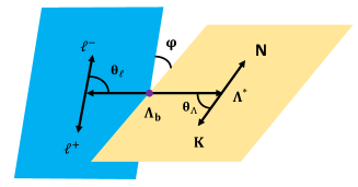
Figure 9: Kinematics of the four-body $\Lambda_{b}\to\Lambda^{\ast}(\to N\bar{K})\ell^{+}\ell^{-}$ decay, where the angles are defined in the corresponding rest frames.

In the following, we will introduce some kinematic conventions that are useful for the calculation of the involved helicity amplitudes.

B.1 Some conventions in $\mathbf{\Lambda_{b}}$ rest frame

In the $\Lambda_{b}$ rest frame, we have the four-momentum of $\Lambda_{b}$, $\Lambda^{\ast}$ and the vector boson as

$$\begin{split}p^{\mu}&=(m_{\Lambda_{b}},0,0,0),\\ k^{\mu}&=(E_{\Lambda^{\ast}},0,0,|\vec{p}_{\Lambda^{\ast}}|),\\ q^{\mu}&=(q_{0},0,0,-|\vec{q}|),\end{split}$$ (B.2)

where

$$\begin{split}E_{\Lambda^{\ast}}&=\frac{m_{\Lambda_{b}}^{2}+m_{\Lambda^{\ast}}^{2}-q^{2}}{2m_{\Lambda_{b}}},~{}~{}~{}|\vec{p}_{\Lambda^{\ast}}|=|\vec{q}|=\frac{\sqrt{s_{+}s_{-}}}{2m_{\Lambda_{b}}},\\ q_{0}&=\frac{m_{\Lambda_{b}}^{2}-m_{\Lambda^{\ast}}^{2}+q^{2}}{2m_{\Lambda_{b}}},~{}~{}~{}s_{\pm}=(m_{\Lambda_{b}}\pm m_{\Lambda^{\ast}})^{2}-q^{2}.\end{split}$$ (B.3)

We have the following solutions for the Dirac spinor of $\Lambda_{b}$ for different $s_{\Lambda_{b}}$ as

$$u_{\Lambda_{b}}(-1/2)=\begin{pmatrix}\sqrt{2m_{\Lambda_{b}}}\\ 0\\ 0\\ 0\\ \end{pmatrix},~{}~{}u_{\Lambda_{b}}(+1/2)=\begin{pmatrix}0\\ \sqrt{2m_{\Lambda_{b}}}\\ 0\\ 0\\ \end{pmatrix},$$ (B.4)

and the solutions for the Rarita-Schwinger spinor $u_{\Lambda^{\ast},\alpha}(s_{\Lambda^{\ast}})$ for different $s_{\Lambda^{\ast}}$ as Descotes-Genon:2019dbw

$$\begin{split}u_{\Lambda^{\ast}}\Big{(}\!-\!\frac{3}{2}\!\Big{)}\!=&\frac{1}{2\sqrt{m_{\Lambda_{b}}}}\!\begin{pmatrix}0&0&0&0\\ 0&\sqrt{s_{+}}&0&-\sqrt{s_{-}}\\ 0&-i\sqrt{s_{+}}&0&i\sqrt{s_{-}}\\ 0&0&0&0\\ \end{pmatrix},\\ u_{\Lambda^{\ast}}\Big{(}\!-\!\frac{1}{2}\!\Big{)}\!=&\frac{\sqrt{s_{-}s_{+}}}{4\!\sqrt{3}m_{\Lambda^{\ast}}m_{\Lambda_{b}}^{3/2}}\!\begin{pmatrix}0&2\!\sqrt{s_{+}}&0&-2\!\sqrt{s_{-}}\\ \frac{2m_{\Lambda^{\ast}}m_{\Lambda_{b}}}{\sqrt{s_{-}}}&0&\frac{2m_{\Lambda^{\ast}}m_{\Lambda_{b}}}{\sqrt{s_{+}}}&0\\ \frac{-2im_{\Lambda^{\ast}}m_{\Lambda_{b}}}{\sqrt{s_{-}}}&0&\frac{-2im_{\Lambda^{\ast}}m_{\Lambda_{b}}}{\sqrt{s_{+}}}&0\\ 0&\frac{s_{-}+s_{+}}{\sqrt{s_{-}}}&0&-\frac{s_{-}+s_{+}}{\sqrt{s_{+}}}\\ \end{pmatrix},\\ u_{\Lambda^{\ast}}\Big{(}\!+\!\frac{1}{2}\!\Big{)}\!=&\frac{\sqrt{s_{-}s_{+}}}{4\!\sqrt{3}m_{\Lambda^{\ast}}m_{\Lambda_{b}}^{3/2}}\!\begin{pmatrix}2\!\sqrt{s_{+}}&0&2\!\sqrt{s_{-}}&0\\ 0&\frac{-2m_{\Lambda^{\ast}}m_{\Lambda_{b}}}{\sqrt{s_{-}}}&0&\frac{2m_{\Lambda^{\ast}}m_{\Lambda_{b}}}{\sqrt{s_{+}}}\\ 0&\frac{-2im_{\Lambda^{\ast}}m_{\Lambda_{b}}}{\sqrt{s_{-}}}&0&\frac{2im_{\Lambda^{\ast}}m_{\Lambda_{b}}}{\sqrt{s_{+}}}\\ \frac{s_{-}+s_{+}}{\sqrt{s_{-}}}&0&\frac{s_{-}+s_{+}}{\sqrt{s_{+}}}&0\\ \end{pmatrix},\\ u_{\Lambda^{\ast}}\Big{(}\!+\!\frac{3}{2}\!\Big{)}\!=&\frac{1}{2\sqrt{m_{\Lambda_{b}}}}\!\begin{pmatrix}0&0&0&0\\ -\sqrt{s_{+}}&0&-\sqrt{s_{-}}&0\\ -i\sqrt{s_{+}}&0&-i\sqrt{s_{-}}&0\\ 0&0&0&0\\ \end{pmatrix},\end{split}$$ (B.5)

where the column and row notations correspond to the spinor indices $\alpha$ and the vector indices, respectively. In addition, the polarization vectors for the virtual vector boson alone on the $-z$ axis in the $\Lambda_{b}$ rest frame are expressed as

$$\begin{split}\epsilon^{\mu}(t)&=\frac{1}{\sqrt{q^{2}}}(q_{0},0,0,-|\vec{q}|),\\ \epsilon^{\mu}(0)&=\frac{1}{\sqrt{q^{2}}}(-|\vec{q}|,0,0,q_{0}),\\ \epsilon^{\mu}(\pm)&=\frac{1}{\sqrt{2}}(0,\mp 1,-i,0),\end{split}$$ (B.6)

where we use $t$ and $0$ to distinguish the two $\lambda_{W}=0$ states ($0$ for $J=1$ and $t$ for $J=0$), and $\pm$ to represent $\lambda_{W}=\pm$ for $J=1$, respectively.

B.2 Some conventions in the dilepton rest frame

In the dilepton rest frame, we have the four-momentum of the vector bosons and leptons as

$$\begin{split}q^{\mu}&=(\sqrt{q^{2}},0,0,0),\\ q_{\ell^{-}}^{\mu}&=(E_{\ell},|\vec{q}_{\ell}|\sin\theta_{\ell},0,|\vec{q}_{\ell}|\cos\theta_{\ell}),\\ q_{\ell^{+}}^{\mu}&=(E_{\ell},-|\vec{q}_{\ell}|\sin\theta_{\ell},0,-|\vec{q}_{\ell}|\cos\theta_{\ell}),\end{split}$$ (B.7)

where $|\vec{q}_{\ell}|=\sqrt{q^{2}}\beta_{\ell}/2$ and $E_{\ell}=\sqrt{q^{2}}/2$. The Dirac spinors for $\ell^{-}$ and $\ell^{+}$ in Dirac representation are

$$\begin{split}u_{\ell^{-}}(\vec{q}_{\ell},s_{\ell^{-}})&=\begin{pmatrix}\sqrt{E_{\ell}+m_{\ell}}\ \chi\left(\vec{q}_{\ell},s_{\ell^{-}}\right)\\ 2s_{\ell^{-}}\sqrt{E_{\ell}-m_{\ell}}\ \chi\left(\vec{q}_{\ell},s_{\ell^{-}}\right)\end{pmatrix},\\ v_{\ell^{+}}(-\vec{q}_{\ell},s_{\ell^{+}})&=\begin{pmatrix}\sqrt{E_{\ell}-m_{\ell}}\ \xi\left(-\vec{q}_{\ell},s_{\ell^{+}}\right)\\ -2s_{\ell^{+}}\sqrt{E_{\ell}+m_{\ell}}\ \xi\left(-\vec{q}_{\ell},s_{\ell^{+}}\right)\end{pmatrix},\end{split}$$ (B.8)

respectively, where

$$\begin{split}&\chi(\vec{q}_{\ell},\frac{1}{2})=\xi(-\vec{q}_{\ell},\frac{1}{2})=\begin{pmatrix}\cos\frac{\theta_{\ell}}{2}\\ \sin\frac{\theta_{\ell}}{2}\end{pmatrix},\\ &\chi(\vec{q}_{\ell},-\frac{1}{2})=-\xi(-\vec{q}_{\ell},-\frac{1}{2})=\begin{pmatrix}-\sin\frac{\theta_{\ell}}{2}\\ \cos\frac{\theta_{\ell}}{2}\end{pmatrix}.\end{split}$$ (B.9)

In addition, the polarization vectors of the virtual vector boson in the dilepton rest frame are written as

$$\begin{split}\bar{\epsilon}^{\mu}(t)&=(1,0,0,0),\\ \bar{\epsilon}^{\mu}(0)&=(0,0,0,1),\\ \bar{\epsilon}^{\mu}(\pm)&=\frac{1}{\sqrt{2}}(0,\mp 1,-i,0),\end{split}$$ (B.10)

which satisfy the following orthogonality and completeness relations Descotes-Genon:2019dbw ; Yan:2019tgn ; Das:2020cpv

$$\bar{\epsilon}^{\ast\mu}(m)\bar{\epsilon}_{\mu}(n) = \tilde{g}_{mn},$$ (B.11)

$$\sum_{m,n}\bar{\epsilon}^{\ast\mu}(m)\bar{\epsilon}^{\nu}(n)\tilde{g}_{mn} = g^{\mu\nu},$$ (B.12)

where $m,n\in\{t,\pm,0\}$, $\tilde{g}_{mn}=\text{diag}(+1,-1,-1,-1)$, and $g^{\mu\nu}=\text{diag}(+1,-1,-1,-1)$.

B.3 Some conventions in $\mathbf{\Lambda^{\ast}}$ rest frame

In the $\Lambda^{\ast}$ rest frame, we have the following solutions for the Rarita-Schwinger spinor $u_{\Lambda^{\ast},\alpha}(s_{\Lambda^{\ast}})$ with different $s_{\Lambda^{\ast}}$ as Descotes-Genon:2019dbw ; Das:2020cpv

$$\begin{split}u_{\Lambda^{\ast}}(-3/2)=&\sqrt{m_{\Lambda^{\ast}}}\begin{pmatrix}0&0&0&0\\ 0&1&0&0\\ 0&-i&0&0\\ 0&0&0&0\\ \end{pmatrix},\\ u_{\Lambda^{\ast}}(-1/2)=&\sqrt{\frac{m_{\Lambda^{\ast}}}{3}}\begin{pmatrix}0&0&0&0\\ 1&0&0&0\\ -i&0&0&0\\ 0&2&0&0\\ \end{pmatrix},\\ u_{\Lambda^{\ast}}(+1/2)=&\sqrt{\frac{m_{\Lambda^{\ast}}}{3}}\begin{pmatrix}0&0&0&0\\ 0&-1&0&0\\ 0&-i&0&0\\ 2&0&0&0\\ \end{pmatrix},\\ u_{\Lambda^{\ast}}(+3/2)=&\sqrt{m_{\Lambda^{\ast}}}\begin{pmatrix}0&0&0&0\\ -1&0&0&0\\ -i&0&0&0\\ 0&0&0&0\\ \end{pmatrix},\end{split}$$ (B.13)

where the column and row notations correspond to the spinor indices $\alpha$ and the vector indices, respectively, and the solutions for the Dirac spinor of the nucleon for different $s_{N}$ as

$$\begin{split}u_{N}(-1/2)=&\frac{1}{2m_{\Lambda^{\ast}}}\begin{pmatrix}-\sqrt{r_{+}}\sin\frac{\theta_{\Lambda^{\ast}}}{2}e^{-i\phi}\\ \sqrt{r_{+}}\cos\frac{\theta_{\Lambda^{\ast}}}{2}\\ \sqrt{r_{-}}\sin\frac{\theta_{\Lambda^{\ast}}}{2}e^{-i\phi}\\ -\sqrt{r_{-}}\cos\frac{\theta_{\Lambda^{\ast}}}{2}\\ \end{pmatrix},\\ u_{N}(+1/2)=&\frac{1}{2m_{\Lambda^{\ast}}}\begin{pmatrix}\sqrt{r_{+}}\cos\frac{\theta_{\Lambda^{\ast}}}{2}\\ \sqrt{r_{+}}\sin\frac{\theta_{\Lambda^{\ast}}}{2}e^{i\phi}\\ \sqrt{r_{-}}\cos\frac{\theta_{\Lambda^{\ast}}}{2}\\ \sqrt{r_{-}}\sin\frac{\theta_{\Lambda^{\ast}}}{2}e^{i\phi}\\ \end{pmatrix}.\end{split}$$ (B.14)

References

- (1) M. Huschle et al. [Belle], Measurement of the branching ratio of relative to decays with hadronic tagging at Belle, Phys. Rev. D 92 (2015) no.7, 072014.
- (2) R. Aaij et al. [LHCb], Measurement of the ratio of branching fractions , Phys. Rev. Lett. 115 (2015) no.11, 111803 [erratum: Phys. Rev. Lett. 115 (2015) no.15, 159901].
- (3) S. Hirose et al. [Belle], Measurement of the lepton polarization and in the decay , Phys. Rev. Lett. 118 (2017) no.21, 211801.
- (4) G. Caria et al. [Belle], Measurement of and with a semileptonic tagging method, Phys. Rev. Lett. 124 (2020) no.16, 161803.
- (5) T. M. Aliev, A. Ozpineci and M. Savci, Exclusive decay beyond standard model, Nucl. Phys. B 649 (2003), 168-188.
- (6) D. Das, On the angular distribution of decay, JHEP 07 (2018), 063.
- (7) T. Aaltonen et al. [CDF], Observation of the Baryonic Flavor-Changing Neutral Current Decay , Phys. Rev. Lett. 107 (2011), 201802.
- (8) R. Aaij et al. [LHCb], Differential branching fraction and angular analysis of decays, JHEP 06 (2015), 115 [erratum: JHEP 09 (2018), 145].
- (9) R. Aaij et al. [LHCb], Angular moments of the decay at low hadronic recoil, JHEP 09 (2018), 146.
- (10) G. Li, C. W. Liu and C. Q. Geng, Bottomed baryon decays with invisible Majorana fermions, [arXiv:2206.01575 [hep-ph]].
- (11) W. Altmannshofer and F. Archilli, [arXiv:2206.11331 [hep-ph]].
- (12) W. Detmold and S. Meinel, form factors, differential branching fraction, and angular observables from lattice QCD with relativistic quarks, Phys. Rev. D 93 (2016) no.7, 074501.
- (13) W. Detmold, C. J. D. Lin, S. Meinel and M. Wingate, form factors and differential branching fraction from lattice QCD, Phys. Rev. D 87 (2013) no.7, 074502.
- (14) C. H. Chen and C. Q. Geng, Lepton asymmetries in heavy baryon decays of , Phys. Lett. B 516 (2001), 327-336.
- (15) M. J. Aslam, Y. M. Wang and C. D. Lü, Exclusive semileptonic decays of in supersymmetric theories, Phys. Rev. D 78 (2008), 114032.
- (16) Y. M. Wang and Y. L. Shen, Perturbative Corrections to Form Factors from QCD Light-Cone Sum Rules, JHEP 02 (2016), 179.
- (17) T. M. Aliev, K. Azizi and M. Savci, Analysis of the decay in QCD, Phys. Rev. D 81 (2010), 056006.
- (18) Y. M. Wang, Y. Li and C. D. Lü, Rare Decays of and in the Light-cone Sum Rules, Eur. Phys. J. C 59 (2009), 861-882.
- (19) Y. M. Wang, Y. L. Shen and C. D. Lü, transition form factors from QCD light-cone sum rules, Phys. Rev. D 80 (2009), 074012.
- (20) T. Gutsche, M. A. Ivanov, J. G. Korner, V. E. Lyubovitskij and P. Santorelli, Rare baryon decays and : differential and total rates, lepton- and hadron-side forward-backward asymmetries, Phys. Rev. D 87 (2013), 074031.
- (21) L. Mott and W. Roberts, Rare dileptonic decays of in a quark model, Int. J. Mod. Phys. A 27 (2012), 1250016.
- (22) L. Mott and W. Roberts, Lepton polarization asymmetries for FCNC decays of the b baryon, Int. J. Mod. Phys. A 30 (2015) no.27, 1550172.
- (23) L. L. Liu, X. W. Kang, Z. Y. Wang and X. H. Guo, Rare decay in the Bethe-Salpeter equation approach, Chin. Phys. C 44 (2020) no.8, 083107.
- (24) H. Yan, Angular distribution of the rare decay , [arXiv:1911.11568 [hep-ph]].
- (25) P. Böer, T. Feldmann and D. van Dyk, Angular Analysis of the Decay , JHEP 01 (2015), 155.
- (26) T. Blake and M. Kreps, Angular distribution of polarised baryons decaying to , JHEP 11 (2017), 138.
- (27) T. Blake, S. Meinel and D. van Dyk, Bayesian Analysis of Wilson Coefficients using the Full Angular Distribution of Decays, Phys. Rev. D 101 (2020) no.3, 035023.
- (28) S. Meinel and G. Rendon, form factors from lattice QCD, Phys. Rev. D 103 (2021) no.7, 074505.
- (29) S. Meinel and G. Rendon, form factors from lattice QCD and improved analysis of the and form factors, Phys. Rev. D 105 (2022) no.5, 054511.
- (30) M. Bordone, Heavy Quark Expansion of (1520) Form Factors beyond Leading Order, Symmetry 13 (2021) no.4, 531.
- (31) S. Descotes-Genon and M. Novoa-Brunet, Angular analysis of the rare decay , JHEP 06 (2019), 136 [erratum: JHEP 06 (2020), 102].
- (32) D. Das and J. Das, The decay at low-recoil in HQET, JHEP 07 (2020), 002.
- (33) G. Hiller and R. Zwicky, Endpoint relations for baryons, JHEP 11 (2021), 073.
- (34) Y. Amhis, M. Bordone and M. Reboud, Dispersive analysis of local form factors, [arXiv:2208.08937 [hep-ph]].
- (35) Z. P. Xing, F. Huang and W. Wang, Angular distributions for Decays, [arXiv:2203.13524 [hep-ph]].
- (36) Y. Amhis, S. Descotes-Genon, C. Marin Benito, M. Novoa-Brunet and M. H. Schune, Prospects for New Physics searches with decays, Eur. Phys. J. Plus 136 (2021) no.6, 614.
- (37) P. Guo, H. W. Ke, X. Q. Li, C. D. Lü and Y. M. Wang, Diquarks and the semi-leptonic decay of in the hyrid scheme, Phys. Rev. D 75 (2007), 054017.
- (38) J. Zhu, Z. T. Wei and H. W. Ke, Semileptonic and nonleptonic weak decays of , Phys. Rev. D 99 (2019) no.5, 054020.
- (39) Z. X. Zhao, Weak decays of heavy baryons in the light-front approach, Chin. Phys. C 42 (2018) no.9, 093101.
- (40) C. K. Chua, Color-allowed bottom baryon to charmed baryon nonleptonic decays, Phys. Rev. D 99 (2019) no.1, 014023.
- (41) C. K. Chua, Color-allowed bottom baryon to -wave and -wave charmed baryon nonleptonic decays, Phys. Rev. D 100 (2019) no.3, 034025.
- (42) H. W. Ke, N. Hao and X. Q. Li, Revisiting and weak decays in the light-front quark model, Eur. Phys. J. C 79 (2019) no.6, 540.
- (43) H. W. Ke, Q. Q. Kang, X. H. Liu and X. Q. Li, Weak decays of in the light-front quark model, Chin. Phys. C 45 (2021) no.11, 113103.
- (44) E. Hiyama, Y. Kino and M. Kamimura, Gaussian expansion method for few-body systems, Prog. Part. Nucl. Phys. 51 (2003), 223-307.
- (45) T. Yoshida, E. Hiyama, A. Hosaka, M. Oka and K. Sadato, Spectrum of heavy baryons in the quark model, Phys. Rev. D 92 (2015) no.11, 114029.
- (46) G. Yang, J. Ping, P. G. Ortega and J. Segovia, Triply heavy baryons in the constituent quark model, Chin. Phys. C 44 (2020) no.2, 023102.
- (47) E. Hiyama and M. Kamimura, Study of various few-body systems using Gaussian expansion method (GEM), Front. Phys. (Beijing) 13 (2018) no.6, 132106.
- (48) G. Buchalla, A. J. Buras and M. E. Lautenbacher, Weak decays beyond leading logarithms, Rev. Mod. Phys. 68, 1125-1144 (1996).
- (49) B. Grinstein, R. P. Springer and M. B. Wise, Effective Hamiltonian for Weak Radiative B Meson Decay, Phys. Lett. B 202, 138-144 (1988).
- (50) Q. S. Yan, C. S. Huang, W. Liao and S. H. Zhu, Exclusive semileptonic rare decays (, in supersymmetric theories, Phys. Rev. D 62 (2000), 094023.
- (51) K. Azizi, S. Kartal, A. T. Olgun and Z. Tavukoglu, Comparative analysis of the semileptonic transition in SM and different SUSY scenarios using form factors from full QCD, JHEP 10 (2012), 118.
- (52) W. J. Li, Y. B. Dai and C. S. Huang, Exclusive semileptonic rare decays in a SUSY SO(10) GUT, Eur. Phys. J. C 40 (2005), 565-577.
- (53) A. Ahmed, I. Ahmed, M. A. Paracha, M. Junaid, A. Rehman and M. J. Aslam, Comparative Study of Decays in Standard Model and Supersymmetric Models, [arXiv:1108.1058 [hep-ph]].
- (54) A. Ali, G. F. Giudice and T. Mannel, Towards a model independent analysis of rare decays, Z. Phys. C 67 (1995), 417-432.
- (55) A. J. Buras and M. Munz, Effective Hamiltonian for beyond leading logarithms in the NDR and HV schemes, Phys. Rev. D 52 (1995), 186-195.
- (56) A. Khodjamirian, T. Mannel, A. A. Pivovarov and Y. M. Wang, Charm-loop effect in and , JHEP 09 (2010), 089.
- (57) A. Khodjamirian, T. Mannel and Y. M. Wang, decay at large hadronic recoil, JHEP 02 (2013), 010.
- (58) P. A. Zyla et al. [Particle Data Group], Review of Particle Physics, PTEP 2020 (2020) no.8, 083C01.
- (59) A. K. Leibovich and I. W. Stewart, Semileptonic decay to excited baryons at order , Phys. Rev. D 57 (1998), 5620-5631.
- (60) T. Feldmann and M. W. Y. Yip, Form factors for transitions in the soft-collinear effective theory, Phys. Rev. D 85, 014035 (2012) [erratum: Phys. Rev. D 86, 079901 (2012)].
- (61) M. Pervin, W. Roberts and S. Capstick, Semileptonic decays of heavy lambda baryons in a quark model, Phys. Rev. C 72 (2005), 035201.
- (62) C. Y. Cheung, W. M. Zhang and G. L. Lin, Light front heavy quark effective theory and heavy meson bound states, Phys. Rev. D 52 (1995), 2915-2925.
- (63) H. Y. Cheng, C. Y. Cheung and C. W. Hwang, Mesonic form-factors and the Isgur-Wise function on the light front, Phys. Rev. D 55 (1997), 1559-1577.
- (64) C. Q. Geng, C. C. Lih and W. M. Zhang, Radiative leptonic B decays in the light front model, Phys. Rev. D 57 (1998), 5697-5702.
- (65) H. Y. Cheng, C. K. Chua and C. W. Hwang, Light front approach for heavy pentaquark transitions, Phys. Rev. D 70 (2004), 034007.
- (66) C. Q. Geng, C. W. Liu and T. H. Tsai, Semileptonic weak decays of antitriplet charmed baryons in the light-front formalism, Phys. Rev. D 103 (2021) no.5, 054018.
- (67) C. Q. Geng, C. W. Liu, Z. Y. Wei and J. Zhang, Weak radiative decays of antitriplet bottomed baryons in light-front quark model, Phys. Rev. D 105 (2022) no.7, 7.
- (68) J. G. Korner, M. Kramer and D. Pirjol, Heavy baryons, Prog. Part. Nucl. Phys. 33 (1994), 787-868.
- (69) F. Hussain, J. G. Korner, J. Landgraf and S. Tawfiq, light diquark symmetry and current induced heavy baryon transition form-factors, Z. Phys. C 69 (1996), 655-662.
- (70) S. Tawfiq, P. J. O’Donnell and J. G. Korner, Charmed baryon strong coupling constants in a light front quark model, Phys. Rev. D 58 (1998), 054010.
- (71) W. Wang and Z. P. Xing, Weak decays of triply heavy baryons in light front approach, [arXiv:2203.14446 [hep-ph]].
- (72) Z. X. Zhao, Weak decays of triply heavy baryons: the case, [arXiv:2204.00759 [hep-ph]].
- (73) Y. S. Li, X. Liu and F. S. Yu, Revisiting semileptonic decays of supported by baryon spectroscopy, Phys. Rev. D 104 (2021) no.1, 013005.
- (74) Y. S. Li and X. Liu, Restudy of the color-allowed two-body nonleptonic decays of bottom baryons and supported by hadron spectroscopy, Phys. Rev. D 105 (2022) no.1, 013003.
- (75) S. Capstick and N. Isgur, Baryons in a Relativized Quark Model with Chromodynamics, AIP Conf. Proc. 132 (1985), 267-271.
- (76) S. Godfrey and N. Isgur, Mesons in a Relativized Quark Model with Chromodynamics, Phys. Rev. D 32 (1985), 189-231.
- (77) S. Q. Luo, L. S. Geng and X. Liu, Double-charm heptaquark states composed of two charmed mesons and one nucleon, Phys. Rev. D 106 (2022), 014017.
- (78) R. Aaij et al. [LHCb], Observation of Two New Excited States Decaying to , Phys. Rev. Lett. 128 (2022) no.16, 162001.
- (79) C. G. Boyd, B. Grinstein and R. F. Lebed, Model independent extraction of using dispersion relations, Phys. Lett. B 353 (1995), 306-312.
- (80) C. Bourrely, I. Caprini and L. Lellouch, Model-independent description of decays and a determination of , Phys. Rev. D 79 (2009), 013008 [erratum: Phys. Rev. D 82 (2010), 099902].
- (81) A. Khodjamirian, T. Mannel, N. Offen and Y. M. Wang, Width and from QCD Light-Cone Sum Rules, Phys. Rev. D 83 (2011), 094031.
- (82) C. B. Lang, D. Mohler, S. Prelovsek and R. M. Woloshyn, Predicting positive parity mesons from lattice QCD, Phys. Lett. B 750 (2015), 17-21.
- (83) N. Isgur and M. B. Wise, Weak Decays of Heavy Mesons in the Static Quark Approximation, Phys. Lett. B 232 (1989), 113-117.
- (84) N. Isgur and M. B. Wise, Weak transition form-factors between heavy mesons, Phys. Lett. B 237 (1990), 527-530.
- (85) N. Isgur and M. B. Wise, Heavy baryon weak form-factors, Nucl. Phys. B 348 (1991), 276-292.
- (86) T. Mannel, W. Roberts and Z. Ryzak, Baryons in the heavy quark effective theory, Nucl. Phys. B 355 (1991), 38-53.
- (87) T. Mannel and Y. M. Wang, Heavy-to-light baryonic form factors at large recoil, JHEP 12 (2011), 067.
- (88) W. Wang, Factorization of Heavy-to-Light Baryonic Transitions in SCET, Phys. Lett. B 708 (2012), 119-126.
- (89) R. Aaij et al. [LHCb], Test of lepton universality with decays, JHEP 05 (2020), 040.