Quantitative unique continuation for wave operators with a jump discontinuity across an interface and applications to approximate control

Abstract

In this article we prove quantitative unique continuation results for wave operators of the form $\partial_{t}^{2}-\textnormal{div}(c(x)\nabla\cdot)$ where the scalar coefficient $c$ is discontinuous across an interface of codimension one in a bounded domain or on a compact Riemannian manifold. We do not make any assumptions on the geometry of the interface or on the sign of the jumps of the coefficient $c$. The key ingredient is a local Carleman estimate for a wave operator with discontinuous coefficients. We then combine this estimate with the recent techniques of Laurent-Léautaud [LL19] to propagate local unique continuation estimates and obtain a global stability inequality. As a consequence, we deduce the cost of the approximate controllability for waves propagating in this geometry.

Keywords

Unique continuation, Carleman estimate, wave equation, jumps across an interface, approximate control, stability estimates

2010 Mathematics Subject Classification: 35B60, 47F05, 35L05, 93B07, 93B05, 35Q93

1 Introduction

For a wave operator $P$ the question of unique continuation consists in asking whether a partial observation of a wave on a small set $\omega$ is sufficient to determine the whole wave. If this property holds, then the next natural question is if we can quantify it. This is expressed via a stability estimate of the form

$$\left\|u\right\|_{\Omega}\lesssim\phi\left(\left\|u\right\|_{\omega},\left\|Pu\right\|_{\Omega},\left\|u\right\|_{\Omega}\right),$$ (1.1)

with $\phi$ satisfying

$$\phi(a,b,c)\stackrel{{\scriptstyle a,b\rightarrow 0}}{{\longrightarrow}}0,\quad\textnormal{with }c\textnormal{ bounded.}$$

Such estimates have numerous applications in control theory, spectral geometry and inverse problems. Concerning the wave operator a seminal unique continuation result was obtained by Robbiano in [Rob91] and refined by Hörmander in [Hör92]. The optimal version of this qualitative result was finally attained in the so called Tataru, Hörmander, Robbiano-Zuily Theorem [Tat95, Tat99, Hör97, RZ98]. This theorem deals in fact with the more general case of operators with partially analytic coefficients and, in the particular case of a wave operator with coefficients independent of time, gives uniqueness across any non characteristic hypersurface. Recently, in [LL19] the authors proved a quantitative version of the latter theorem which, for the wave equation, is optimal with respect to the observation time and the stability estimate obtained. Note that, a qualitative uniqueness result is equivalent to an approximate controllability result, and a quantified version of it gives an estimate of the control cost. The quantitative unique continuation result of [LL19] applies to (variants of) the operator $\partial_{t}^{2}-\Delta_{g}$ where $\Delta_{g}$ is an elliptic operator with $C^{\infty}$ coefficients. See also [BKL16] for a related set of estimates concerning the wave operator.

However, in many contexts, waves propagate through singular media and therefore in the presence of non smooth coefficients. E.g. in the case of seismic waves [Sym83] or acoustic waves [YDdH⁺17, AdHG17, CdHKU19] propagating through the Earth’s crust. Models proposing to describe such phenomena use discontinuous metrics and more precisely metrics which are piece-wise regular but presenting jumps along some hypersurfaces. See for instance the Mohorovičić discontinuity between the Earth’s crust and the mantle. Another example arises in medical imaging. The human brain [FdLKBH01, MCCP17] has two main components: white and grey matter. These two have very different electric conductivities and models describing the situation are very similar to the preceding example.

The question of quantitative unique continuation across a jump discontinuity seems to be well understood in the elliptic/parabolic context. One of the first results (in the parabolic case) is [DOP02] where the operator $\partial^{2}_{t}-\textnormal{div}(c\nabla\cdot)$ is studied with a monotonicity assumption imposed on the scalar coefficient $c=c(x)$: the observation should take place in the region where the coefficient $c$ is smaller. In this article a global Carleman estimate was proved. Later, in the elliptic case in [LR10] a similar result was obtained but without any restriction on the sign of the jump of the coefficient. These techniques were extended to the parabolic context in [LR11]. The most recent (and general) result to the best of our knowledge is proved by Le Rousseau and Lerner [LRL13] where the anisotropic case ($-\textnormal{div}(A(x)\nabla\cdot)$, with $A$ a matrix jumping across an interface) is treated.

The question of exact control for waves with jumps at an interface has already been addressed in the book [Lio88]. A controllability result is proved for the operator $\partial_{t}^{2}-\textnormal{div}(c\nabla\cdot)$ with $c$ a piece-wise constant coefficient under a geometric assumption on the jump hypersurface and a sign condition on the jump. One of the first Carleman estimates was proved in the discontinuous setting in [BMO07]. With the same assumption on the coefficient and assuming that the interface is convex the authors prove linear quantitative stability estimates. Recently, in [BGM21] quantitative results were proved as well for interfaces that interpolate between star-shaped and convex. Other related works are [Gag18] and [BCDCG20].

However, to our knowledge the question of stability estimates without any particular geometric assumption on the interface has not been studied yet. This is the main object of this article.

1.1 Setting and statement of main results

Let $(\mathcal{M},g)$ be a smooth connected compact $n$-dimensional Riemannian manifold with or without boundary. We consider $S$ an $(n-1)$-dimensional submanifold of $\mathcal{M}$ without boundary. We assume that $\mathcal{M}\backslash S=\Omega_{-}\cup\Omega_{+}$ with $\Omega_{-}\cap\Omega_{+}=\emptyset$.

We consider a scalar coefficient $c(x)=\mathds{1}_{\Omega_{-}}c_{-}(x)+\mathds{1}_{\Omega_{+}}c_{+}(x)$ with $c_{\pm}\in C^{\infty}(\overline{\Omega}_{\pm})$ satisfying $0<c_{\min}<c(x)<c_{\max}$ uniformly on $\Omega_{-}\cup\Omega_{+}$ to ensure ellipticity. We shall work with the wave operator $P$ defined as

$$P=\partial^{2}_{t}-\textnormal{div}_{g}(c(x)\nabla_{g}),\quad\textnormal{on }\mathbb{R}_{t}\times\Omega_{-}\cup\Omega_{+}.$$ (1.2)

We consider for $(u_{0},u_{1})\in H^{1}_{0}(\mathcal{M})\times L^{2}(\mathcal{M})$ the following evolution problem:

$$\begin{cases}Pu=0&\textnormal{in}\>(0,T)\times\Omega_{-}\cup\Omega_{+}\\ u_{|S_{-}}=u_{|S_{+}}&\textnormal{in}\>(0,T)\times S\\ (c\partial_{\nu}u)_{|S_{-}}=(c\partial_{\nu}u)_{|S_{+}}&\textnormal{in}\>(0,T)\times S\\ u=0&\textnormal{in}\>(0,T)\times\partial\mathcal{M}\\ \left(u,\partial_{t}u\right)_{|t=0}=(u_{0},u_{1})&\textnormal{in}\>\mathcal{M},\end{cases}$$ (1.3)

where we denote by $\partial_{\nu}$ a nonvanishing vector field defined in a neighborhood of $S$, normal to $S$ (for the metric $g$), pointing into $\Omega_{+}$ and normalized for $g$. We denote as well by $u_{|S_{\pm}}$ the traces of $u_{|\Omega_{\pm}}$ on the hypersurface $S$.

Notice that there are two extra equations in our system. These are some natural transmission conditions that we impose in the interface. These conditions imply that the underlying elliptic operator is self-adjoint on its domain and one can show using classical methods (for instance with the Hill-Yosida Theorem) that the system (1.3) is well posed. For more details on this we refer to Section 2.

Our first result provides a quantitative unique continuation result from an observation region $\omega$ for the discontinuous wave operator $P$.

In section 1.3 we introduce $\mathcal{L}(\mathcal{M},\omega)=\sup_{x\in\mathcal{M}}\textnormal{dist}(x,\omega),$ the “largest distance” of the subset $\omega$ to a point of $\mathcal{M}$, where dist is a distance function adapted to $(\mathcal{M},g,c)$.

Theorem 1.1.

Consider $(\mathcal{M},g),S,\Omega_{\pm}$ and $P$ as defined in (1.2). Then for any nonempty open subset $\omega$ of $\mathcal{M}$ and any $T>2\mathcal{L}(\mathcal{M},\omega)$, there exist $C,\kappa,\mu_{0}$ such that for any $(u_{0},u_{1})\in H^{1}_{0}(\mathcal{M})\times L^{2}(\mathcal{M})$ and $u$ solving (1.3) one has, for any $\mu\geq\mu_{0}$,

$$\left\|(u_{0},u_{1})\right\|_{L^{2}\times H^{-1}}\leq Ce^{\kappa\mu}\left\|u\right\|_{L^{2}((0,T)\times\omega)}+\frac{C}{\mu}\left\|(u_{0},u_{1})\right\|_{H^{1}\times L^{2}}.$$

If moreover $\partial\mathcal{M}\neq\emptyset$ and $\Gamma$ is a non empty open subset of $\partial\mathcal{M}$, for any $T>2\mathcal{L}(\mathcal{M},\Gamma)$, there exist $C,\kappa,\mu_{0}>0$ such that for any $(u_{0},u_{1})\in H^{1}_{0}(\mathcal{M})\times L^{2}(\mathcal{M})$ and $u$ solving (1.3), we have

$$\left\|(u_{0},u_{1})\right\|_{L^{2}\times H^{-1}}\leq Ce^{\kappa\mu}\left\|\partial_{\nu_{\Gamma}}u\right\|_{L^{2}((0,T)\times\Gamma)}+\frac{C}{\mu}\left\|(u_{0},u_{1})\right\|_{H^{1}\times L^{2}}.$$

Remark 1.2.

In fact one can take $\mu>0$ in the statement of the above theorem. However we preferred to state it in this way in order to stress out the fact that this estimate is interesting only when $\mu$ is large.

With the above one can recover the following qualitative result: “If we do not see anything from $\omega$ during a time $T$ strictly larger than $2\mathcal{L}(\mathcal{M},\omega)$, then there is no wave at all.” Indeed, if $\left\|u\right\|_{L^{2}((0,T)\times\omega)}=0$, then letting $\mu\rightarrow+\infty$ in the above inequality implies that $(u_{0},u_{1})=0$.

An important aspect of this theorem is that there is no assumption on the sign of the jump of the coefficient $c$ and consequently the observation region $\omega$ can be chosen indifferently on $\Omega_{-}$ or $\Omega_{+}$. Let us explain why this is quite surprising. Suppose, to fix ideas, that $c_{-}<c_{+}$ are two constants. We can then interpret $c_{-}$ and $c_{+}$ as the the speed of propagation of a wave travelling through two isotropic media $\Omega_{-}$ and $\Omega_{+}$ with different refractive indices, $n_{-}$ and $n_{+}$ respectively (recall that $n_{\pm}=1/c_{\pm}$). Imagine that a wave starts travelling from a region that is inside $\Omega_{-}$. One has $\frac{c_{-}}{c_{+}}=\frac{n_{+}}{n_{-}}$ and therefore the assumption $c_{-}<c_{+}$ translates to $n_{-}>n_{+}$. Then Snell-Descartes law states that when a wave travels from a medium with a higher refractive index to one with a lower refractive index there is a critical angle from which there is total internal reflection, that is no refraction at all. At the level of geometric optics, that is to say, in the high frequency regime such a wave stays trapped inside $\Omega_{-}$. Therefore one expects that, at least at high frequency, no information propagates from $\Omega_{-}$ to $\Omega_{+}$, following the laws of geometric optics. Our result (see Theorem 1.3) states that the intensity of waves in $\Omega_{+}$ is at least exponentially small in terms of the typical frequency $\Lambda$ of the wave.

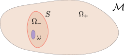
(a) The observation takes place inside $\Omega_{-}$.

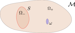
(b) The observation takes place inside $\Omega_{+}$. If $c_{-}<c_{+}$ then a part of the wave may be trapped inside $\Omega_{-}$. Nevertheless, the quantitative unique continuation and its consequences still hold.

We can reformulate Theorem 1.1 in a way closer to quantitative estimates such as (1.1). Indeed, optimizing the inequalities of Theorem 1.1 with respect to $\mu$ yields the following result (which we state only in the interior observation case):

Theorem 1.3.

Under the assumptions of Theorem 1.1 there exists $C>0$ such that for all $(u_{0},u_{1})\in H^{1}_{0}(\mathcal{M})\times L^{2}(\mathcal{M})$ with $(u_{0},u_{1})\neq(0,0)$ one has:

$$\left\|(u_{0},u_{1})\right\|_{H^{1}\times L^{2}} \leq Ce^{C\Lambda}\left\|u\right\|_{L^{2}((0,T)\times\omega)},$$

$$\left\|(u_{0},u_{1})\right\|_{L^{2}\times H^{-1}} \leq C\frac{\left\|(u_{0},u_{1})\right\|_{H^{1}\times L^{2}}}{\log\left(1+\frac{\left\|(u_{0},u_{1})\right\|_{H^{1}\times L^{2}}}{\left\|u\right\|_{L^{2}((0,T)\times\omega)}}\right)}.$$ (1.4)

where $\Lambda=\frac{\left\|(u_{0},u_{1})\right\|_{H^{1}\times L^{2}}}{\left\|(u_{0},u_{1})\right\|_{L^{2}\times H^{-1}}}$.

Note that $\Lambda$ represents the typical frequency of the initial data. Theorem 1.3 is a direct consequence of Theorem 1.1 and Lemma A.3 in [LL19]. Notice that the function

$$x\mapsto\frac{1}{\log(1+1/x)},$$

appearing in the right hand side of (1.3) has been tacitly extended by continuity by $0$ when $x=0$.

In [Rob95, proof of Theorem 2, Section 3] it is shown that such a quantitative information can lead to an estimate for the cost of the approximate controllability. We state the case of internal control, a similar result holds for approximate boundary controllability as well.

Theorem 1.4 (Cost of approximate interior control).

Consider $\mathcal{M}$, $S$ and $\omega\subset\mathcal{M}$ as before. Then for any $T>2\mathcal{L}(\mathcal{M},\omega)$ there exist $C,c>0$ such that for any $\epsilon>0$ and any $(u_{0},u_{1})\in H^{1}_{0}(\mathcal{M})\times L^{2}(\mathcal{M})$, there exists $f\in L^{2}((0,T)\times\omega)$ with

$$\left\|f\right\|_{L^{2}((0,T)\times\omega)}\leq Ce^{c/\epsilon}\left\|(u_{0},u_{1})\right\|_{H^{1}_{0}(\mathcal{M})\times L^{2}(\mathcal{M})}$$

such that the solution of

$$\begin{cases}Pu=\mathds{1}_{\omega}f&\textnormal{in}\>(0,T)\times\Omega_{-}\cup\Omega_{+}\\ u_{|S_{-}}=u_{|S_{+}}&\textnormal{in}\>(0,T)\times S\\ (c\partial_{\nu}u)_{|S_{-}}=(c\partial_{\nu}u)_{|S_{+}}&\textnormal{in}\>(0,T)\times S\\ u=0&\textnormal{in}\>(0,T)\times\partial\mathcal{M}\\ \left(u,\partial_{t}u\right)_{|t=0}=(u_{0},u_{1})&\textnormal{in}\>\mathcal{M},\end{cases}$$

satisfies

$$\left\|(u,\partial_{t}u)_{|t=T}\right\|_{L^{2}\times H^{-1}}\leq\epsilon\left\|(u_{0},u_{1})\right\|_{H^{1}_{0}\times L^{2}}.$$

In other words, if we act on the region $\omega$ during a time $T>2\mathcal{L}(\mathcal{M},\omega)$ we can drive our solution from energy $1$ (in $H^{1}\times L^{2}$) to $\epsilon$ close to $0$ (in $L^{2}\times H^{-1}$). Additionally, this comes with an estimate of the energy of the control which is of the order of $e^{c/\epsilon}$. In the analytic context and without the presence of an interface it was shown in [Leb92] that this form of exponential cost is optimal in the absence of Geometric Control Condition [BLR92].

In the more general hypoelliptic context of [LL21] the result of Theorem 1.4 is stated as approximate observability for the wave equation. It is shown by the authors of this article that such a property implies some resolvent estimates (Proposition 1.11 in [LL21]) which in turn give a logarithmic energy decay estimate for the damped wave equation (see Theorem 1.5 in [LL21]). Consequently, Theorem 1.4 combined with the results of [LL21] provides a different proof for theorems that were already obtained using Carleman estimates for elliptic/parabolic operators (see [LR10] or [LRL13]).

Remark 1.5.

We have assumed that the interface $S$ decomposes $\mathcal{M}$ in two disjoint parts $\Omega_{+}$ and $\Omega_{-}$. However the same results can be obtained for other more general geometric situations as well. This comes from the fact that the key ingredient is a local quantitative estimate (see Theorem 5.1). See also the figure in [LRLR13, Section 1.3.2]

1.2 Strategy of the proof and organization of the paper

1.2.1 The Carleman estimate

One of the main tools for dealing with problems of local unique continuation across a hypersurface $\{\phi=0\}$ is Carleman estimates. The idea, introduced by Carleman in [Car39], is to prove an inequality involving a weight function $\psi$ and a large parameter $\tau$, of the form

$$\left\|e^{\tau\psi}Pu\right\|_{L^{2}}\gtrsim\left\|e^{\tau\psi}u\right\|_{L^{2}},\quad\tau\geq\tau_{0},$$

uniform in $\tau$. The weight function $\psi$ is closely related to the level sets of the function $\phi$ which defines implicitly the hypersurface. In an heuristic way, the chosen weight re-enforces the sets where $u$ is zero and propagates smallness from sets where $\psi$ is big to sets where $\psi$ is small. Since Carleman estimates are already quantitative in nature they provide a good starting point for results of the form (1.1). We point out the fact that this is a local problem. In order to obtain a global result one needs in general to propagate the local one by passing through an appropriate family of hypersurfaces.

The core of this article is to prove a local Carleman estimate in a neighborhood of the interface, containing a microlocal weight in the spirit of [Tat95, Hör97, RZ98]. The presence of discontinuous coefficients complicates significantly this task. In general, for a Carleman estimate to hold a condition involving the principal symbol of the operator and the hypersurface needs to hold, the so-called pseudoconvexity condition (see for instance [Hör67]). These results are based on microlocal analysis arguments and some regularity is necessary for the estimate to hold. In our case we explicitly construct an appropriate weight function and show our estimate for this particular weight. Our proof is inspired by that of Lerner-Le Rousseau in the elliptic case [LRL13] and relies in a factorization argument. Even though the behavior of our (hyperbolic) operator may be very different we consider in our context the wave operator as a “perturbation” of a Laplacian, in the spirit of [Tat95, Hör97, RZ98, LL19]. Let us explain why. For the sake of exposition, consider that $\mathcal{M}=\mathbb{R}^{n}$, $g$ is the Euclidean metric and $c$ is piecewise constant with a jump across the hypersurface $S=\{x_{n}=0\}$. That is $c=c_{+}\mathds{1}_{\{x_{n}>0\}}+c_{-}\mathds{1}_{\{x_{n}<0\}}$. Then the principal symbol of the wave operator $\Box=\partial_{t}^{2}-c\Delta$ is

$$\sigma(\Box)=-\xi^{2}_{t}+c|\xi|^{2}.$$

The inequality we want to prove contains the weight $e^{-\epsilon\frac{D^{2}_{t}}{2\tau}}$ which heuristically localizes close to $\{\xi_{t}=0\}$, in other words localizes in a microlocal region where our operator is close to being elliptic.

In order to obtain a Carleman estimate with a weight $\psi$ one obtains an inequality for the conjugated operator $P_{\psi}$ defined by $P_{\psi}:=e^{\tau\psi}Pe^{-\tau\psi}$. In [LRL13] the authors use an idea which can be traced back to Calderón [Cal58]. They factorize the conjugated operator $P_{\psi}$ as a product of two first-order operators and prove estimates for each first order factor. In the elliptic case $P=-c\Delta$ and for a weight $\psi$ depending only on $x_{n}$ one has the following factorization:

$$P_{\psi} =c_{+}\left(D_{n}+i(\tau\psi^{\prime}+|\xi^{\prime}|)\right)\left(D_{n}+i(\tau\psi^{\prime}-|\xi^{\prime}|)\right)$$

$$\hskip 11.38109pt+c_{-}\left(D_{n}+i(\tau\psi^{\prime}-|\xi^{\prime}|)\right)\left(D_{n}+i(\tau\psi^{\prime}+|\xi^{\prime}|\right)$$

$$=c_{+}\left(D_{n}+ie_{+}\right)\left(D_{n}+if_{+}\right)+c_{-}\left(D_{n}+if_{-}\right)\left(D_{n}+ie_{-}\right).$$

Here the operator has been identified with its symbol in the tangential variables. This allows to work on the normal variable $x_{n}$ and treat the other ones as parameters. In more technical terms, we can use the tools of tangential symbolic calculus in all the variables but $x_{n}$ and try to obtain good one-dimensional estimates for the first order operators $D_{n}+ie_{\pm}$ and $D_{n}+if_{\pm}$. The general principle is that the sign of $e_{\pm},f_{\pm}$ determines the quality of the one dimensional estimates. The choice of the weight function $\psi$ is made so that the following key property is satisfied: we can cover the tangential dual space by $\Gamma_{1}$, $\Gamma_{2}$ such that $(x^{\prime},\tau,\xi^{\prime})\in\mathbb{R}^{n-1}\times\mathbb{R}\times\mathbb{R}^{n-1}=\Gamma_{1}\cup\Gamma_{2}$ with $f_{+}\geq 0$ on $\Gamma_{1}$ and $f_{-}\leq 0$ on $\Gamma_{2}$.

In the proof of the present article, in which $P$ is a wave operator, we work essentially in two microlocal zones. In the first zone, the operator $P$ is not microlocally elliptic. In this zone, we consider terms involving $D_{t}$ as admissible errors. Using the operator $e^{-\epsilon\frac{D^{2}_{t}}{2\tau}}$ allows us then to obtain the desired estimate. In the second zone, the operator $P$ is microlocally elliptic one can follow the proof provided in the elliptic case in [LRL13].

In Section 2 we give the precise statement of the local Carleman estimate that we prove and we describe adapted local coordinates in a small neighborhood of the interface to prepare the proof. In Section 4 we prove the Carleman estimate. We considered helpful to give first a proof for a toy model (constant coefficients case) in Section 3. In this case one can simply work on the Fourier domain without having to work with pseudodifferential operators (see  [Ler19, Chapter 10]). At the same time it allows to understand the core of the arguments which will be used in the general case too.

1.2.2 Using the Carleman estimate

The next step is to use the Carleman estimate. To do this, one needs to obtain a local quantitative version which can be iterated. This has been done in the smooth case by Laurent and Léautaud in [LL19]. There, the estimate has the same form as that obtained in [LL19] in a (arbitrarily small) neighborhood of the interface $S$. Thus, we are able to use it “once” to pass on the other side of $S$ and then combine it with the results of [LL19]. In Section 5.1 we show how one can use the techniques of [LL19] to obtain such a local quantitative estimate in a neighborhood of the interface where the coefficients jump. Finally in Section 5.3 we prove that indeed, one can propagate the quantitative estimate by combining our local estimate with the analogous results in the smooth case.

1.3 Some notations and definitions

We recall in this Section some elementary geometric facts and we give the precise definition of the distance which is used in the statement of Theorem 1.1 and Theorem 1.4.

Let us recall that the geometric setting is given at the beginning of Section 1.1. The interface $S$ has a natural metric given by the restriction of $g$ to $TS$. In local coordinates we have:

$$\partial_{\nu}=\sum_{j}\nu^{j}\partial_{x_{j}},\quad\nu^{j}=\lambda\sum_{k}n_{k}g^{jk},\quad|\nu_{g}|=1,$$

with $g^{ij}g_{jk}=\delta_{ik},$ $\lambda^{2}=\left(\sum_{i,j}g^{ij}n_{i}n_{j}\right)^{-1}$ and $n$ is the normal to $S$ for the Euclidean metric in the chosen local coordinates pointing into $\Omega_{+}$. We denote by $(\cdot,\cdot)_{g}=g(\cdot,\cdot)$ the inner product on $T\mathcal{M}$. The Riemannian gradient of a function $f$ is defined in an intrinsic manner by

$$(\nabla_{g}f,X)_{g}=df(X),\quad\textnormal{for any smooth vector field }X.$$

The integral of a function $f$ is defined by $\int f:=\int_{\mathcal{M}}f(x)d\textnormal{Vol}_{g}(x)$, where $d\textnormal{Vol}_{g}(x)$ is the Riemannian volume element. The divergence operator, acting on a vector field $X$ is defined by the relation

$$\int u\textnormal{ div}_{g}X=-\int(\nabla_{g}u,X)_{g},\quad\textnormal{for all }u\in C^{\infty}_{0}(\textnormal{Int}\mathcal{M}).$$

Let us recall the expression of these objects in local coordinates. We consider $f$ a smooth function on $\mathcal{M}$ and $X=\sum_{i}X^{i}\partial_{x_{i}}$, $Y=\sum_{i}Y^{i}\partial_{x_{i}}$ two smooth vector fields on $\mathcal{M}$. We have:

$$(X,Y)_{g} =\sum_{i,j}g_{ij}X^{i}Y^{j},\quad\nabla_{g}f=\sum_{i,j}g^{ij}(\partial_{j}f)\partial_{x_{i}},\quad\textnormal{div}_{g}(X)=\frac{1}{\sqrt{\det g}}\sum_{i}\partial_{i}\left(\sqrt{\det g}X_{i}\right).$$

We finally have:

$$\textnormal{div}_{g}(c(x)\nabla_{g}f)=\frac{1}{\sqrt{\det g}}\sum_{i,j}\partial_{x_{i}}\left(cg^{ij}\sqrt{\det g}\partial_{x_{j}}f\right),\quad x\in\Omega_{-}\cup\Omega_{+}.$$

We want to define the natural distance associated to the operator $P$ appearing in Theorem 1.1. Consider the piecewise smooth metric $g_{c}$ by $g_{c}:=\mathds{1}_{\Omega_{-}}c^{-1}_{-}g+\mathds{1}_{\Omega_{+}}c^{-1}_{+}g$.

Definition 1.

An admissible path $C^{\infty}([0,1];\mathcal{M})\ni\gamma:[0,1]\rightarrow\mathcal{M}$ is a path satisfying the conditions:

• $\gamma$ does not have self-intersections

• $\gamma$ intersects the interface $S$ a finite number of times

• $\gamma(t)\in S\Longrightarrow\gamma^{\prime}(t)\perp T_{\gamma(t)}S$

In particular, if $\gamma$ is an admissible path then the map $t\mapsto|\gamma^{\prime}(t)|_{g_{c}(\gamma(t))}\in L^{\infty}([0,1];\mathcal{M})$ is bounded and consequently we can define its length by the usual formula:

$$\textnormal{length}(\gamma)=\int_{0}^{1}|\gamma^{\prime}(t)|_{g_{c}(\gamma(t))}dt.$$

We now define the distance we will be working with:

Definition 2.

The distance of two points $x_{0},x_{1}\in\mathcal{M}$ is defined as:

$$\textnormal{dist}(x_{0},x_{1})=\inf\{\textnormal{length}(\gamma)|\>\>\gamma\textnormal{ admissible path, }\gamma(0)=x_{0},\gamma(1)=x_{1}\}.$$

We can now as well define the largest distance of a subset $E\subset\mathcal{M}$ to $\mathcal{M}$ by

$$\mathcal{L}(\mathcal{M},E):=\sup_{x\in\mathcal{M}}\textnormal{dist}(x,E),$$ (1.5)

where

$$\textnormal{dist}(x,E)=\inf_{y\in E}\textnormal{dist}(x,y).$$

Remark 1.6.

Notice that the conditions imposed on the family of admissible paths do not pose any important restriction since any Lipschitz path can be replaced by an admissible one up to increasing its length by an $\epsilon>0$ arbitrarily small. Since we take the infimum of these lengths the distance remains the same.

Acknowledgements The author would like to thank C. Laurent and M. Léautaud for introducing him to the problem as well as for discussions, encouragements, and patient guidance.

2 The Carleman estimate

The key ingredient for the proof of Theorem 1.1 is a local Carleman estimate. Since we will work in space-time it is convenient to consider $\Sigma:=\mathbb{R}_{t}\times S$ with $S$ the smooth interface of the manifold $\mathcal{M}$ defined in Section 1.1. Therefore, $\Sigma$ is a smooth hypersurface of $\mathbb{R}_{t}\times\mathcal{M}.$ We define as well $\Omega_{t,\pm}:=\mathbb{R}_{t}\times\Omega_{\pm}$.

2.1 General transmission conditions

We want to derive a Carleman estimate for the wave operator

$$\Box=P:=\partial_{t}^{2}-\textnormal{div}_{g}(c(x)\nabla_{g}),$$

where the scalar coefficient $c$ satisfies $0<c_{\min}<c(x)<c_{\max}<+\infty$ uniformly for $x\in\Omega_{-}\cup\Omega_{+}$ to make sure that the ellipticity property is satisfied. We recall as well that $c_{|\Omega_{t,\pm}}\in C^{\infty}(\overline{\Omega}_{t,\pm})$ but it jumps across the interface $S$. Since the operator $P$ has discontinuous coefficients one needs to be careful with its domain. Indeed, given a function $u=1_{\Omega_{t,-}}u_{-}+1_{\Omega_{t,+}}u_{+}$ with $u_{\pm}\in C^{\infty}(\mathbb{R}_{t}\times\mathcal{M})$ one has in the distributional sense

$$\nabla_{g}u=1_{\Omega_{t,-}}\nabla_{g}u_{-}+1_{\Omega_{t,+}}\nabla_{g}u_{+}+(u_{-}-u_{+})\delta_{\Sigma}\nu,$$

where $\delta_{\Sigma}$ is the surface measure on $\Sigma$ and $\nu$ is the unit normal vector field pointing into $\Omega_{t,+}$. We impose then that

$$u_{-}{{}_{|\Sigma}}=u_{+}{{}_{|\Sigma}},$$ (2.1)

and the singular term is removed. Similarly, calculating

$$\textnormal{div}(c(x)\nabla_{g}u),$$

we see that the condition

$$c_{+}\partial_{\nu}{u_{+}}_{|\Sigma}=c_{-}\partial_{\nu}{u_{-}}_{|\Sigma}$$ (2.2)

combined with (2.1) gives the equality

$$\textnormal{div}_{g}(c(x)\nabla_{g}u)=1_{\Omega_{t,-}}\textnormal{div}(c_{-}\nabla_{g}u_{-})+1_{\Omega_{t,+}}\textnormal{div}(c_{+}\nabla_{g}u_{+}).$$

We define then $\mathcal{W}$ as the space containing functions of the form

$$u=1_{\Omega_{t,-}}u_{-}+1_{\Omega_{t,+}}u_{+},$$ (2.3)

with $u_{\pm}\in C^{\infty}_{0}(\mathbb{R}_{t}\times\mathcal{M})$ and such that (2.1) and (2.2) hold. These conditions are called transmission conditions and for $u\in\mathcal{W}$ one has $Pu\in L^{2}$. The above calculations show as well that $P$ is formally self adjoint on this domain and therefore by classical methods (energy estimates or semi-group theory) one has that the evolution problem (1.3) is well posed.

Remark 2.1.

The first transmission condition expresses the continuity across the interface and the second one the continuity for the normal flux. Notice that the second condition excludes many smooth functions from the space $\mathcal{W}$. On the other hand elements of $\mathcal{W}$ are Lipschitz continuous and in particular one has $\mathcal{W}\subset H^{1}$.

For technical reasons it will be useful to work with non-homogeneous transmission conditions as well. More precisely, we shall denote by $\mathcal{W}^{\theta,\Theta}$ the space of functions of the form (2.3) satisfying additionally the following non homogeneous transmission conditions:

$${u_{-}}_{|\Sigma} ={u_{+}}_{|\Sigma}+\theta$$ (2.4)

$$c_{+}\partial_{\nu}{u_{+}}_{|\Sigma} =c_{-}\partial_{\nu}{u_{-}}_{|\Sigma}+\Theta,$$ (2.5)

where $\theta$ and $\Theta$ are smooth functions of the interface $\Sigma$.

2.2 Local setting in a neighborhood of the interface

Since we show a local Carleman estimate we can state it directly in adapted local coordinates. In a sufficiently small neighborhood $V$ of a point $x_{0}$ of $S$ one can use normal geodesic coordinates with respect to the spatial variables $x$ (see [Hör85], Appendix C.5, [LRLR22] Section 9.4 ). In such a coordinate system the interface $S$ is given by $S=\{x_{n}=0\}$ and the principal part of the operator $P$ denoted by $P_{2}$ takes the form (on both sides of the interface)

$$P_{2}=\partial_{t}^{2}-c(x)(\partial^{2}_{x_{n}}-r(x,\partial_{x^{\prime}}/i)),$$

with $r(x,\xi^{\prime})$ a $x$family of second order polynomials in $\xi^{\prime}$ that satisfy

$$r(x,\xi^{\prime})\in\mathbb{R},\quad C_{1}|\xi^{\prime}|^{2}\leq r(x,\xi^{\prime})\leq C_{2}|\xi^{\prime}|^{2},$$

for $x\in V$, $\xi^{\prime}\in\mathbb{R}^{n-1}$ and $0<C_{1}<C_{2}<\infty$. The transmission conditions become after this change of variables:

$${u_{-}}_{|x_{n}=0} ={u_{+}}_{|x_{n}=0}+\theta$$ (2.6)

$$c_{+}\partial_{x_{n}}{u_{+}}_{|x_{n}=0} =c_{-}\partial_{x_{n}}{u_{-}}_{|x_{n}=0}+\Theta,$$ (2.7)

In this setting, the two sides of the interface become $\Omega_{t,+}=\{x_{n}>0\}$ and $\Omega_{t,-}=\{x_{n}<0\}$. We shall use the notation

$$H_{\pm}=1_{\Omega_{t,\pm}}.$$

and we have for the coefficient $c:$

$$c(x)=H_{-}c_{-}(x)+H_{+}c_{+}(x).$$

The space $\mathcal{W}^{\theta,\Theta}$ consists in this local context of functions $u$ of the form

$$u=H_{-}u_{-}+H_{+}u_{+},\quad u_{\pm}\in C^{\infty}_{0}(\mathbb{R}_{t}\times V),$$

satisfying also (2.6) and (2.7). We define as well

$$P^{\pm}:=\partial_{t}^{2}-\text{div}(c_{\pm}\nabla\cdot).$$

Following [Tat95, Hör97, RZ98] we are seeking to prove a Carleman estimate containing the microlocal weight

$$Q_{\delta,\tau}^{\phi}=e^{-\frac{\delta|D_{t}|^{2}}{2\tau}}e^{\tau\phi}.$$ (2.8)

We shall take $\phi$ in the following form:

$$\phi=\phi(x_{n})=\left(\alpha_{-}x_{n}+\frac{\beta x_{n}^{2}}{2}\right)H_{-}+\left(\alpha_{+}x_{n}+\frac{\beta x_{n}^{2}}{2}\right)H_{+},\quad\alpha_{\pm},\beta>0.$$ (2.9)

The parameters $\alpha_{\pm}$ and $\beta$ will be chosen in the sequel. The parameter $\beta$ will be taken large and is related to the sub-ellipticity property (see for instance [Hör63] or [Hör94]) which is necessary for a Carleman estimate to hold. The choice of $\alpha_{\pm}$ comes from the construction in the microlocally elliptic case (see Lemma 4.11). It is a geometric condition on the interface that requires the jump of $\partial_{x_{n}}\phi$ (i.e. $\alpha_{+}-\alpha_{-}>0$) to be sufficiently large (see 4.32).

The following is our main Carleman estimate and its proof will occupy a large part of this article:

Theorem 2.2.

In the geometric situation presented just above let $(t_{0},x_{0})\in\mathbb{R}_{t}\times V$. Then there exists an appropriate weight $\phi$ and some positive constants $C$, $\tau_{0}$, $\delta$, $d$, $r_{0}$ such that

$$C\left\|H_{-}Q_{\delta,\tau}^{\phi}P^{-}u_{-}\right\|_{L^{2}}^{2}+C\left\|H_{+}Q_{\delta,\tau}^{\phi}P^{+}u_{+}\right\|_{L^{2}}^{2}\\ +Ce^{-d\tau}\left(\tau^{3}\left\|e^{\tau\phi}u\right\|_{L^{2}}^{2}+\tau\left\|H_{+}\nabla e^{\tau\phi}u_{+}\right\|_{L^{2}}^{2}+\tau\left\|H_{-}\nabla e^{\tau\phi}u_{-}\right\|_{L^{2}}^{2}\right)+CT_{\theta,\Theta}\\ \geq\tau^{3}\left\|Q_{\delta,\tau}^{\phi}u\right\|_{L^{2}}^{2}+\tau\left\|H_{+}\nabla Q_{\delta,\tau}^{\phi}u_{+}\right\|_{L^{2}}^{2}+\tau\left\|H_{-}\nabla Q_{\delta,\tau}^{\phi}u_{-}\right\|_{L^{2}}^{2},$$

for $u\in\mathcal{W}^{\theta,\Theta}$ such that $\operatorname{supp}u\subset B((t_{0},x_{0}),r_{0})$ and $\tau\geq\tau_{0}$, where

$$T_{\theta,\Theta}=\tau^{3}\left|Q_{\delta,\tau}^{\phi}\theta\right|_{L^{2}(\Sigma)}^{2}+\tau\left|Q_{\delta,\tau}^{\phi}\nabla\theta\right|_{L^{2}(\Sigma)}^{2}+\tau\left|Q_{\delta,\tau}^{\phi}\Theta\right|_{L^{2}(\Sigma)}^{2}.$$ (2.10)

Several remarks are in order:

Remark 2.3.

Observe that the choice of $\phi$ is well adapted to the geometric situation: for small $|x_{n}|$ we have that $\Sigma=\{x_{n}=0\}=\{\phi=0\}$ and the two sides of the interface are given by $\{\phi>0\}$ and $\{\phi<0\}$. We also have (for $|x_{n}|$ sufficiently small) that $\phi^{\prime}>0$, and consequently $\phi$ is larger in $\Omega^{+}$: $\Omega^{+}$ is the observation region and the Carleman estimate of Theorem 2.2 will propagate uniqueness from $\Omega^{+}$ to $\Omega^{-}$. In particular, the weight function $\phi$ is suitable for observation in the sense of [LRL13, Property (1-12)].

Remark 2.4.

Notice that in the case of homogeneous transmission conditions $\theta=\Theta=0$ one has $T_{\theta,\Theta}=0$. The calculations carried out in Section 2.1 imply that $Pu\in L^{2}$ and therefore

$$\left\|H_{-}P^{-}u_{-}\right\|_{L^{2}}+\left\|H_{+}P^{+}u_{+}\right\|_{L^{2}}=\left\|Pu\right\|_{L^{2}}.$$

Using moreover the fact that $u\in H^{1}$ we can write the estimate of Theorem 2.2 in a more concise way as:

$$C\left(\left\|Q_{\delta,\tau}^{\phi}Pu\right\|_{L^{2}}^{2}+e^{-d\tau}\left\|e^{\tau\phi}u\right\|_{H^{1}_{\tau}}^{2}\right)\geq\tau\left\|Q_{\delta,\tau}^{\phi}u\right\|_{H^{1}_{\tau}}^{2},$$

where the $\left\|\cdot\right\|_{H^{1}_{\tau}}$ norm is defined as

$$\left\|w\right\|_{H^{1}_{\tau}}:=\tau\left\|w\right\|_{L^{2}}+\left\|\nabla w\right\|_{L^{2}}.$$

Remark 2.5.

As in [LRL13] we explicitly construct an appropriate weight function $\phi$. It will initially depend only in the variable $x_{n}$ with $\Sigma=\{x_{n}=0\}$. In Section 4.5 we shall use a perturbation argument to allow dependence upon the other variables as well.

As usual, to prove Theorem 2.2 we work with the conjugated operator $P_{\phi,\delta}$ defined in our case by the relation:

$$e^{-\frac{\delta|D_{t}|^{2}}{2\tau}}e^{\tau\phi}P^{\pm}=P^{\pm}_{\phi,\delta}e^{-\frac{\delta|D_{t}|^{2}}{2\tau}}e^{\tau\phi}.$$ (2.11)

For a general weight $\phi$ the operators $P^{\pm}_{\phi,\delta}$ do not exist, however in the case where $\phi$ is quadratic in $t$ one can show that we have the following expression for $P^{\pm}_{\phi,\delta}$ (see for instance [Hör97, Chapter 2]):

$$P^{\pm}_{\phi,\delta} =c_{\pm}(x)(D_{n}+i\tau\phi^{\prime}-\delta\kappa^{\prime\prime}_{t,t}D_{t})^{2}+c_{\pm}(x)\sum_{1\leq j,k\leq n-1}b_{jk}(x)(D_{j}+i\tau\partial_{j}\phi-\delta\phi^{\prime\prime}_{t,x_{j}})(D_{k}+i\tau\partial_{k}\phi-\delta\phi^{\prime\prime}_{t,x_{k}})$$

$$\hskip 11.38109pt-(D_{t}+i\tau\phi^{\prime}_{t}-\delta\phi^{\prime\prime}_{t,t}D_{t})^{2}$$ (2.12)

This will be used at a later stage where we will convexify our initial weight $\phi$ as we know that this is in general a necessary procedure for our Carleman estimate to be used if one wishes to obtain qualitative or quantitative uniqueness results. We shall however initially consider a weight $\phi$ depending solely on the variable $x_{n}$, and a perturbation argument will be used to allow some convexification. In the case where $\phi$ is independent of $t$ the conjugated operator $e^{\tau\phi}Pe^{-\tau\phi}$ commutes with the Fourier multiplier $e^{-\frac{\delta D^{2}_{t}}{2\tau}}$ and it takes the following particularly simple form:

$$P^{\pm}_{\phi}=c_{\pm}(x)(D_{n}+i\tau\phi^{\prime})^{2}+c_{\pm}(x)\sum_{1\leq j,k\leq n-1}b_{jk}(x)D_{j}D_{k}-D_{t}^{2}$$

As for the smooth case shown by Tataru we will prove a sub elliptic estimate concerning the conjugated operator, which will act on functions of the form $w=Q_{\delta,\tau}^{\phi}u$ for $u\in\mathcal{W}^{\theta,\Theta}$. We therefore have to understand the action of the conjugated operator on the transmission conditions. We use the following expressions:

$$w_{\pm}(t,x) =\left(\frac{\tau}{2\pi\delta}\right)^{\frac{1}{2}}\int_{\mathbb{R}}e^{-\frac{\tau}{2\delta}(t-s)^{2}}e^{\tau\phi}u_{\pm}(s,x)ds$$

$$\partial_{n}w_{\pm}(t,x) =\left(\frac{\tau}{2\pi\delta}\right)^{\frac{1}{2}}\int_{\mathbb{R}}e^{-\frac{\tau}{2\delta}(t-s)^{2}}e^{\tau\phi}\left(\tau\phi^{\prime}_{\pm}u_{\pm}+\partial_{n}u_{\pm}\right)(s,x)ds.$$

Let us define

$$V_{t}:=\mathbb{R}_{t}\times V.$$ (2.13)

One has that $u\in\mathcal{W}^{\theta,\Theta}$ is equivalent to $w\in\mathcal{W}^{\theta,\Theta}_{\phi}$ with the space $\mathcal{W}^{\theta,\Theta}_{\phi}$ being defined as the space containing functions $w$ such that

$$w=H_{-}w_{-}+H_{+}w_{+},\quad w_{\pm}\in C^{\infty}_{0}(V_{t}),$$

satisfying additionally the following modified transmission conditions:

$${w_{-}}_{|\Sigma} ={w_{+}}_{|\Sigma}+\theta_{\phi}$$ (2.14)

$$c_{+}\left(D_{n}{w_{+}}+i\tau\alpha_{+}w_{+}\right)_{|\Sigma} =c_{-}\left(D_{n}{w_{-}}+i\tau\alpha_{-}w_{-}\right)_{|\Sigma}+\Theta_{\phi},$$ (2.15)

where $\theta_{\phi}=Q_{\delta,\tau}^{\phi}\theta$ and $\Theta_{\phi}=Q_{\delta,\tau}^{\phi}\Theta$. The following proposition is the main step in the proof of Theorem 2.2:

Proposition 2.6.

Let $(t_{0},x_{0})\in\Sigma$. There exist a suitable weight $\phi$ and $C,\tau_{0},r_{0}>0$ such that

$$C\bigg{(}\left\|P^{-}_{\phi}v_{-}\right\|_{L^{2}(\mathbb{R}^{n+1})}^{2}+\left\|P^{+}_{\phi}v_{+}\right\|_{L^{2}(\mathbb{R}^{n+1})}^{2}+\tau\left\|H_{+}D_{t}v_{+}\right\|_{L^{2}(\mathbb{R}^{n+1})}^{2}+\tau\left\|H_{-}D_{t}v_{-}\right\|_{L^{2}(\mathbb{R}^{n+1})}^{2}\\ +\tau\left|(D_{t}v_{+})_{|\Sigma}\right|^{2}_{L^{2}(\Sigma)}+\tau\left|(D_{t}v_{-})_{|\Sigma}\right|^{2}_{L^{2}(\Sigma)}+T_{\theta,\Theta}\bigg{)}\\ \geq\tau^{3}\left\|v\right\|_{L^{2}(\mathbb{R}^{n+1})}^{2}+\tau\left\|H_{+}\nabla v_{+}\right\|_{L^{2}(\mathbb{R}^{n+1})}^{2}+\tau\left\|H_{-}\nabla v_{-}\right\|_{L^{2}(\mathbb{R}^{n+1})}^{2}\\ +\tau^{3}\left|v_{+}\right|_{L^{2}(\Sigma)}^{2}+\tau^{3}\left|v_{-}\right|_{L^{2}(\Sigma)}^{2}+\tau\left|(\nabla v_{+})_{|\Sigma}\right|_{L^{2}(\Sigma)}^{2}+\tau\left|(\nabla v_{-})_{|\Sigma}\right|_{L^{2}(\Sigma)}^{2},$$

for $v\in\mathcal{W}^{\theta,\Theta}_{\phi}$ such that $\operatorname{supp}v\subset B((t_{0},x_{0}),r_{0})$ and $\tau\geq\tau_{0}$.

Proposition 2.6 provides a sub elliptic estimate for the conjugated operator which contains an admissible error (compared to a standard Carleman estimate) in its left hand side, which we will call $E_{t}$ for convenience in the sequel:

$$E_{t}(v):=\tau\left\|H_{+}D_{t}v_{+}\right\|_{L^{2}(\mathbb{R}^{n+1})}^{2}+\tau\left\|H_{-}D_{t}v_{-}\right\|_{L^{2}(\mathbb{R}^{n+1})}^{2}\\ +\tau\left|(D_{t}v_{+})_{|\Sigma}\right|^{2}_{L^{2}(\Sigma)}+\tau\left|(D_{t}v_{-})_{|\Sigma}\right|^{2}_{L^{2}(\Sigma)}.$$ (2.16)

2.3 Proof of Theorem 2.2 from Proposition 2.6

One should notice that Theorem 2.2 is not a straightforward consequence of Proposition 2.6. Indeed when one considers $w=Q_{\delta,\tau}^{\phi}u$ the function $w$ is not necessarily compactly supported even though this is the case for $u$ and consequently Proposition 2.6 cannot be applied directly. In particular when we pass from Proposition 2.6 to Theorem 2.2 the Gaussian weight localizes close to $\{D_{t}=0\}$ and that is why $E_{t}$ is an admissible remainder term. Nevertheless the passage from Proposition 2.6 to Theorem 2.2 is quite classical ([Tat95, Hör97]). In our context one has additionally to deal with the terms coming from the interface. Let us present a proof here:

Proof that Proposition 2.6 implies Theorem 2.2.

We consider an element $u\in\mathcal{W}^{\theta,\Theta}$ satisfying additionally

$$\operatorname{supp}{u}\subset B(0,r/4),$$

with $r:=\frac{r_{0}}{2}$ and $r_{0}$ fixed by Proposition 2.6. We define as before $w=Q^{\phi}_{\delta,\tau}u=e^{-\frac{\delta|D_{t}|^{2}}{2\tau}}e^{\tau\phi}u$ which is not compactly supported on the time variable $t$. We take then $\zeta\in C^{\infty}_{0}((-r,r);[0,1])$ with $\zeta=1$ on $(-r/2,r/2)$. This implies that the function $v:=\zeta(t)w(t,x)\in\mathcal{W}^{\theta,\Theta}_{\phi}$ satisfies additionally $\operatorname{supp}{v}\subset B(0,r_{0})$ which means that we can apply Proposition 2.6 to it. We neglect the last two surface terms and write the estimate of Proposition 2.6 in a more compact and slightly weaker form to obtain:

$$\sum_{\pm}\left(\left\|H_{\pm}P^{\pm}_{\phi}v\right\|_{L^{2}}^{2}+\tau\left\|H_{\pm}D_{t}v_{\pm}\right\|_{L^{2}}^{2}+\tau\left|D_{t}v_{\pm}\right|_{L^{2}(\Sigma)}^{2}+T_{\zeta\theta,\zeta\Theta}\right)\gtrsim\tau\left\|v\right\|_{H^{1}_{\tau}}^{2}+\tau^{3}\left|v_{\pm}\right|_{L^{2}(\Sigma)}^{2}.$$

Using the fact that $\zeta(t)\leq 1$, the definition of $T_{\theta,\Theta}$ in (2.10) and the property (B.1) of $Q_{\delta,\tau}^{\phi}$ we see that $T_{\zeta\theta,\zeta\Theta}\leq CT_{\theta,\Theta}$. This yields:

$$\sum_{\pm}\left(\left\|H_{\pm}P^{\pm}_{\phi}v\right\|_{L^{2}}^{2}+\tau\left\|H_{\pm}D_{t}v_{\pm}\right\|_{L^{2}}^{2}+\tau\left|D_{t}v_{\pm}\right|_{L^{2}(\Sigma)}^{2}+T_{\theta,\Theta}\right)\gtrsim\tau\left\|v\right\|_{H^{1}_{\tau}}^{2}+\tau^{3}\left|v_{\pm}\right|_{L^{2}(\Sigma)}^{2}.$$ (2.17)

Now we estimate for $w$:

$$\tau\left\|v\right\|_{H^{1}_{\tau}}^{2}+\tau^{3}\left|w_{\pm}\right|_{L^{2}(\Sigma)}^{2} \lesssim\tau\left\|\zeta w\right\|_{H^{1}_{\tau}}^{2}+\tau\left\|(1-\zeta)w\right\|_{H^{1}_{\tau}}^{2}+\tau^{3}\left|\zeta w_{\pm}\right|_{L^{2}(\Sigma)}^{2}+\tau^{3}\left|(1-\zeta)w_{\pm}\right|_{L^{2}(\Sigma)}^{2}$$

$$\lesssim\sum_{\pm}\left(\left\|H_{\pm}P^{\pm}_{\phi}\zeta w\right\|_{L^{2}}^{2}+\tau\left\|H_{\pm}D_{t}\zeta w_{\pm}\right\|_{L^{2}}^{2}+\tau\left|D_{t}\zeta w_{\pm}\right|_{L^{2}(\Sigma)}^{2}+T_{\theta,\Theta}\right)$$

$$\hskip 11.38109pt+\tau\left\|(1-\zeta)w\right\|_{H^{1}_{\tau}}^{2}+\tau^{3}\left|(1-\zeta)w_{\pm}\right|_{L^{2}(\Sigma)}^{2},$$ (2.18)

thanks to (2.17). For the last two terms we remark that

$$(1-\zeta)w=(1-\zeta)e^{-\frac{\delta|D_{t}|^{2}}{2\tau}}e^{\tau\phi}u=(1-\zeta)e^{-\frac{\delta|D_{t}|^{2}}{2\tau}}(\check{\chi}e^{\tau\phi}u),$$

with $\check{\chi}=\check{\chi}(t)\in C^{\infty}_{0}((-r/3,r/3))$ with $\check{\chi}=1$ in a neighborhood of $[-r/4,r/4]$ which implies that $\check{\chi}u=u$. Since $1-\zeta$ is supported away from $(-r/2,r/2)$ one can apply Lemma B.2 which gives:

$$\tau\left\|(1-\zeta)w\right\|_{H^{1}_{\tau}}^{2}+\tau^{3}\left|(1-\zeta)w_{\pm}\right|_{L^{2}(\Sigma)}^{2}\leq C\tau e^{-c\frac{\tau}{\delta}}\left\|e^{\tau\phi}u\right\|_{H^{1}_{\tau}}^{2}+C\tau^{3}e^{-c\frac{\tau}{\delta}}\left|e^{\tau\phi}u_{\pm}\right|_{L^{2}(\Sigma)}^{2}.$$

Therefore it remains to estimate the following three terms, appearing in the right hand side of (2.3):

• We take a function $\tilde{\chi}=\tilde{\chi}(t)$ such that $\tilde{\chi}=1$ on $\operatorname{supp}(\zeta^{\prime})$ and $\tilde{\chi}=0$ on $(-r/3,r/3)$ and find for the first one:

  $$\sum_{\pm}\left\|H_{\pm}P^{\pm}_{\phi}\zeta w\right\|_{L^{2}}^{2} \lesssim\sum_{\pm}\left(\left\|H_{\pm}\zeta P^{\pm}_{\phi}w\right\|_{L^{2}}^{2}+\left\|H_{\pm}[P^{\pm}_{\phi},\zeta]w\right\|_{L^{2}}^{2}\right)$$

  $$\lesssim\sum_{\pm}\left(\left\|H_{\pm}P^{\pm}_{\phi}w\right\|_{L^{2}}^{2}+\left\|H_{\pm}[P^{\pm}_{\phi},\zeta]w\right\|_{L^{2}}^{2}\right)$$

  $$=\sum_{\pm}\left(\left\|H_{\pm}P^{\pm}_{\phi}w\right\|_{L^{2}}^{2}+\left\|H_{\pm}[P^{\pm}_{\phi},\zeta]\tilde{\chi}w\right\|_{L^{2}}^{2}\right)$$

  $$\lesssim\sum_{\pm}\left\|H_{\pm}P^{\pm}_{\phi}w\right\|_{L^{2}}^{2}+\left\|\tilde{\chi}w\right\|_{H^{1}_{\tau}}^{2}$$

  $$\lesssim\sum_{\pm}\left\|H_{\pm}P^{\pm}_{\phi}w\right\|_{L^{2}}^{2}+e^{-c\frac{\tau}{\delta}}\left\|e^{\tau\phi}u\right\|_{H^{1}_{\tau}}^{2}$$ (2.19)

  where we used the properties of the support of $\tilde{\chi}$ and $u$ combined with Lemma B.2.

• For the second term we have, using the support of $\zeta^{\prime}$, as well (to alleviate notation we drop the $\pm$):

  $$\tau\left\|D_{t}\zeta w\right\|_{L^{2}}^{2} \lesssim\tau\left\|\zeta^{\prime}w\right\|_{L^{2}}^{2}+\tau\left\|D_{t}w\right\|_{L^{2}}^{2}$$

  $$\lesssim\tau e^{-c\frac{\tau}{\delta}}\left\|e^{\tau\phi}u\right\|_{L^{2}}^{2}+\tau\left\|D_{t}w\right\|_{L^{2}}^{2}.$$

  To estimate $\tau\left\|D_{t}w\right\|_{L^{2}}^{2}$ we work on the Fourier domain (with respect to the time variable $t$) and distinguish between the frequencies smaller or bigger than $\sigma\tau$ for an arbitrary $\sigma>0$ (as in [LL19, Section 5.2]). One has:

  $$\left\|D_{t}w\right\|_{L^{2}} \leq\left\|1_{|D_{t}|\leq\sigma\tau}D_{t}w\right\|_{L^{2}}+\left\|1_{|D_{t}|\geq\sigma\tau}D_{t}w\right\|_{L^{2}}$$

  $$=\left\|1_{|D_{t}|\leq\sigma\tau}D_{t}w\right\|_{L^{2}}+\left\|1_{|D_{t}|\geq\sigma\tau}D_{t}e^{-\frac{\delta|D_{t}|^{2}}{2\tau}}e^{\tau\phi}u\right\|$$

  $$\leq\left\|1_{|D_{t}|\leq\sigma\tau}D_{t}w\right\|_{L^{2}}+\underset{\xi_{t}\geq\sigma\tau}{\textnormal{max}}\left(\xi_{t}e^{-\frac{\delta\xi^{2}_{t}}{2\tau}}\right)\left\|e^{\tau\phi}u\right\|_{L^{2}}.$$

  We see that if $\tau\geq\frac{1}{\sigma^{2}\delta}$ the function $s\mapsto se^{-\frac{\delta s^{2}}{2\tau}}$ is decreasing on the interval $[\sigma\tau,+\infty)$. We obtain therefore for $\tau\geq\textnormal{max}(\tau_{1},\frac{1}{\sigma^{2}\delta})$ the estimate:

  $$\tau\left\|D_{t}w\right\|_{L^{2}}^{2}\lesssim\sigma^{2}\tau^{3}\left\|w\right\|_{L^{2}}^{2}+\sigma^{2}\tau^{3}e^{-\tau\sigma^{2}\delta}\left\|e^{\tau\phi}u\right\|_{L^{2}}^{2}.$$ (2.20)

  Above and in the sequel the hidden constant will be independent of $\sigma$.

• For the third term $\tau\left|D_{t}\zeta w_{\pm}\right|_{L^{2}(\Sigma)}^{2}$ in (2.3) one can proceed exactly as above to find:

  $$\tau\left|D_{t}\zeta w\right|_{L^{2}(\Sigma)}^{2}\lesssim\tau e^{-c\frac{\tau}{\delta}}\left|e^{\tau\phi}u\right|_{L^{2}(\Sigma)}^{2}+\sigma^{2}\tau^{3}\left|w\right|_{L^{2}(\Sigma)}^{2}+\sigma^{2}\tau^{3}e^{-\tau\sigma^{2}\delta}\left|e^{\tau\phi}u\right|_{L^{2}(\Sigma)}^{2}.$$ (2.21)

We inject estimates (• ‣ 2.3), (2.20) and (2.21) in the right hand side of (2.3) to obtain:

$$\tau\left\|w\right\|_{H^{1}_{\tau}}^{2}+\tau^{3}\left|w\right|_{L^{2}(\Sigma)}^{2} \lesssim\left\|P_{\phi}w\right\|_{L^{2}}^{2}+\left(\tau e^{-c\frac{\tau}{\delta}}+\sigma^{2}\tau^{3}e^{-\tau\sigma^{2}\delta}\right)\left\|e^{\tau\phi}u\right\|_{H^{1}_{\tau}}^{2}$$

$$\hskip 11.38109pt+\left(\tau^{3}e^{-c\frac{\tau}{\delta}}+\sigma^{2}\tau^{3}e^{-\tau\sigma^{2}\delta}\right)\left|e^{\tau\phi}u\right|_{L^{2}(\Sigma)}^{2}$$

$$\hskip 11.38109pt+\sigma^{2}\tau^{3}\left\|w\right\|_{L^{2}}^{2}+\sigma^{2}\tau^{3}\left|w\right|_{L^{2}(\Sigma)}^{2}+T_{\theta,\Theta}.$$

We now choose $\sigma$ sufficiently small to absorb the last two terms above in the left hand side of our estimate. Then there exists $d>0$ such that for $\tau\geq\max(\tau_{0},\frac{1}{\sigma^{2}\delta})$:

$$\sum_{\pm}\left(\tau\left\|w_{\pm}\right\|_{H^{1}_{\tau}}^{2}+\tau^{3}\left|w_{\pm}\right|_{L^{2}(\Sigma)}^{2}\right) \lesssim\sum_{\pm}\left(\left\|H_{\pm}P^{\pm}_{\phi}w_{\pm}\right\|_{L^{2}}^{2}+e^{-d\tau}\left(\left\|e^{\tau\phi}u_{\pm}\right\|_{H^{1}_{\tau}}^{2}+\left|e^{\tau\phi}u_{\pm}\right|_{L^{2}(\Sigma)}^{2}\right)+T_{\theta,\Theta}\right)$$

$$\lesssim\sum_{\pm}\left(\left\|H_{\pm}P^{\pm}_{\phi}w_{\pm}\right\|_{L^{2}}^{2}+e^{-d\tau}\left\|e^{\tau\phi}u_{\pm}\right\|_{H^{1}_{\tau}}^{2}+T_{\theta,\Theta}\right)$$

$$\lesssim\sum_{\pm}\left(\left\|H_{\pm}Q_{\delta,\tau}^{\phi}P^{\pm}u_{\pm}\right\|_{L^{2}}^{2}+e^{-d\tau}\left\|e^{\tau\phi}u_{\pm}\right\|_{H^{1}_{\tau}}^{2}+T_{\theta,\Theta}\right),$$

where we have used the trace estimate $\left|e^{\tau\phi}u\right|_{L^{2}(\Sigma)}^{2}\lesssim\left\|e^{\tau\phi}u\right\|_{H^{1}}^{2}$ as well as the definition of the conjugated operator $P_{\phi}$. This concludes the proof of Theorem 2.2 from Proposition 2.6. ∎

3 Proof of Proposition 2.6 for a toy model

The goal of this section is to prove the subelliptic estimate of Proposition 2.6 in the particular situation where the coefficient $c$ is piecewise constant. This case works as a sketch of proof since it is technically simpler but at the same time it allows to understand the core of the arguments that will be used for the proof of the general case in Section 4.

Notations: Before going further let us fix some useful notations that will be used in the sequel. We write $\mathbb{R}^{n+1}_{+}=\{x_{n}>0\}\times\mathbb{R}^{n}$ with the analogous definition for $\mathbb{R}^{n+1}_{-}$. In particular $\mathbb{R}_{+}$ will refer to $\{x_{n}>0\}$ and $\mathbb{R}_{-}$ to $\{x_{n}<0\}$. We note $\big{(}a,b\big{)}$ the inner product in $L^{2}(\mathbb{R}^{n+1})$ and $x^{\prime}=(x_{1},...,x_{n-1})$. The inner product on $L^{2}(\mathbb{R}^{n+1}_{+}),L^{2}(\mathbb{R}^{n+1}_{-}),\Sigma$ will de denoted by $(\cdot,\cdot)_{+},(\cdot,\cdot)_{-},(\cdot,\cdot)_{\Sigma}$ respectively. When we consider norms on $\Sigma$ the argument will automatically be considered to be restricted in $\Sigma$, even though we shall not always write $|\Sigma$ to simplify our notation. We will simply write $\hat{v}$ for the partial Fourier transform of $v$ in the variables $(t,x^{\prime})$, whose dual variables are $(\xi_{t},\xi^{\prime})$. We recall that the space of functions $\mathcal{W}^{\theta,\Theta}_{\phi}$ and the small neighborhood $V$ have been defined in Section 2.2. To alleviate notation we denote

$$\mathcal{W}_{\phi}:=\mathcal{W}_{\phi}^{0,0},$$

for the case of homogeneous transmission conditions.

We recall that we work in the setting introduced in Section 2.2. We suppose additionally only in this section that the coefficient $c$ is piecewise constant. We write then $c=H_{-}c_{-}+H_{+}c_{+}$ with $c_{\pm}>0$ constants and we consider homogeneous transmission conditions $\theta=\Theta=0$. This allows to write $v_{-}(0)=v_{+}(0)=v(0)$ for $v\in\mathcal{W}_{\phi}$ and it implies as well that $P_{\phi}v\in L^{2}(V_{t})$.

3.1 Factorization and first estimates

In the sequel when we use the notation $\lesssim$ or $\gtrsim$ the implicit constant will depend on the coefficients of $P_{\phi}$ (here $c_{\pm}$) and on the coefficients $\alpha_{\pm},\beta$ of our weight function $\phi$. The constants denoted by $C$ will depend on the same variables and they can be different from one line to another.

In the elliptic case of [LRL13] the authors use a factorization argument which takes advantage of the fact that $-\Delta$ is positive and therefore one can define its square root. In our proof of Proposition 2.6 we use and extend this idea of factorization, however as we no longer have the positivity property this factorization is not always possible. Before giving the details let us observe that we can identify the operator $P_{\phi}$ with its symbol in the tangential variables $(t,x^{\prime})$. Indeed, using Plancherel’s theorem and denoting by $\mathcal{F}_{t,x^{\prime}}$ the partial Fourier transform in the variables $(t,x^{\prime})$ we have:

$$(2\pi)^{n/2}\left\|P_{\phi}v\right\|_{L^{2}(\mathbb{R}^{n+1})} =\left\|\mathcal{F}_{t,x^{\prime}}P_{\phi}v\right\|_{L^{2}(\mathbb{R}^{n+1})}$$

$$=\left\|H_{+}\left(c_{+}(D_{n}+i\tau\phi^{\prime})^{2}+c_{+}|\xi^{\prime}|^{2}-\xi_{t}^{2}\right)\mathcal{F}_{t\rightarrow\xi_{t},x^{\prime}\rightarrow\xi^{\prime}}v_{+}\right\|_{L^{2}(\mathbb{R}^{n+1})}$$

$$\hskip 11.38109pt+\left\|H_{-}\left(c_{-}(D_{n}+i\tau\phi^{\prime})^{2}+c_{-}|\xi^{\prime}|^{2}-\xi_{t}^{2}\right)\mathcal{F}_{t\rightarrow\xi_{t},x^{\prime}\rightarrow\xi^{\prime}}v_{-}\right\|_{L^{2}(\mathbb{R}^{n+1})}.$$

Here we used the fact that the coefficients of $P$ (and thus of $P_{\phi}$ since $\phi=\phi(x_{n})$) are constant. In the general case, although this identification is no longer valid, symbolic calculus will allow to exploit the core of the arguments carried out below. We write:

$$P_{\phi}^{\pm}=c_{\pm}\left((D_{n}+i\tau\phi^{\prime})^{2}+|\xi^{\prime}|^{2}-\frac{1}{c_{\pm}}|\xi_{t}|^{2}\right).$$

For $\epsilon>0$ small to be chosen, we distinguish the following regions of the tangential frequency space $\mathbb{R}^{n}\ni(\xi^{\prime},\xi_{t})$:

1. $\mathcal{E^{\pm}_{\epsilon}}:$ $${|{\xi }^{\prime }|}^2-c_{\pm }^{-1}{|{\xi }_t|}^2\ge ϵ({|{\xi }^{\prime }|}^2+{|{\xi }_t|}^2)$$. This is the elliptic region. Here we can factorize in precisely the same way as in the elliptic case [LRL13] with the same estimates for the first order factors. For $(\xi_{t},\xi^{\prime})\in\mathcal{E^{-}_{\epsilon}}\cap\mathcal{E^{+}_{\epsilon}}$ we can proceed exactly as in the elliptic case.

2. $\mathcal{GH^{\pm}_{\epsilon}}:$ $${|{\xi }^{\prime }|}^2-c_{\pm }^{-1}{|{\xi }_t|}^2<ϵ({|{\xi }^{\prime }|}^2+{|{\xi }_t|}^2)$$. This is the union of the hyperbolic and glancing regions (see for instance [Hör85, Chapter 23.2] or [GL20]). The important fact is that here we have for sufficiently small $\epsilon$ that $|\xi_{t}|\gtrsim|\xi^{\prime}|$. Since $\left\|D_{t}v\right\|=\left\|\xi_{t}v\right\|$ and $|D_{t}v|=|\xi_{t}v|$ are admissible remainder terms (in view of the statement of Proposition 2.6) we obtain directly a useful estimate on all tangential derivatives. It thus only remains to obtain an estimate on $\left\|D_{n}v\right\|$ and $|D_{n}v|$.

We have thus considered two regions adapted to the geometry in each side of the interface (that is $\{x_{n}<0\}$ and $\{x_{n}>0\}$). This gives us four regions which cover all of the tangent dual space. Note that making an assumption on the sign of the jump could reduce the number of regions one has to deal with but we do not make such an assumption.

The following simple Lemma will be used in multiple occasions in the sequel:

Lemma 3.1.

One has for $v\in\mathcal{W}_{\phi}$ and all $\tau>0$:

$$\tau|D_{n}\hat{v}_{\pm}(0)|^{2}\lesssim\tau|D_{n}\hat{v}_{\mp}(0)|^{2}+\tau^{3}|\hat{v}(0)|^{2}$$

This means that if we have one of the two terms $\tau\left|D_{n}\hat{v}_{+}\right|_{L^{2}(\Sigma)}^{2}$ or $\tau\left|D_{n}\hat{v}_{-}\right|_{L^{2}(\Sigma)}^{2}$ we automatically have the other one too, modulo the surface term $\tau^{3}|\hat{v}|^{2}$.

Proof.

This is a result of the transmission conditions (2.14) and (2.15) and of the fact that partial Fourier transform commutes with restriction on $\Sigma=\{x_{n}=0\}$. The first transmission condition allows to write $\hat{v}_{-}(0)=\hat{v}_{+}(0)=\hat{v}(0)$ and (2.15) reads

$$D_{n}\hat{v}_{-}(0)=\frac{c_{+}}{c_{-}}(D_{n}\hat{v}_{+}+i\tau\alpha_{+}\hat{v}_{+}(0))-i\tau\alpha_{-}\hat{v}_{-}(0),$$

and therefore

$$|c_{-}D_{n}\hat{v}_{-}(0)-c_{+}D_{n}\hat{v}_{+}(0)|\lesssim\tau|\hat{v}(0)|,$$

from which the Lemma follows. ∎

Consequently, if for instance one has $\left\|P_{\phi}v\right\|_{L^{2}(\mathbb{R}^{n+1})}^{2}+E_{t}(v)\gtrsim\tau\left|D_{n}v_{-}\right|_{L^{2}(\Sigma)}^{2}+\tau^{3}|v(0)|_{L^{2}(\Sigma)}^{2}$ then thanks to Lemma 3.1 we have:

$$\tau|D_{n}v_{+}(0)|_{L^{2}(\Sigma)}^{2}\lesssim\tau|D_{n}v_{-}(0)|_{L^{2}(\Sigma)}^{2}+\tau^{3}|v(0)|_{L^{2}(\Sigma)}^{2}\lesssim\left\|P_{\phi}v\right\|_{L^{2}(\mathbb{R}^{n+1})}^{2}+E_{t}(v).$$

As we aim at proving a Carleman estimate (which involves a large parameter $\tau$) we expect that regions depending on $\tau$ arise. The following lemma furnishes such a region which is rather favorable:

Lemma 3.2.

For all $\tau,c_{0}>0$, $v\in\mathcal{W}_{\phi}$ and $Y\subset\{|\xi_{t}|\geq c_{0}(\tau+|\xi^{\prime}|)\}$ one has

$$\tau\left\|\widehat{D_{t}v_{+}}\right\|_{L^{2}(\mathbb{R}_{+}\times Y)}^{2}+\tau\left\|\widehat{D_{t}v_{-}}\right\|_{L^{2}(\mathbb{R}_{-}\times Y)}^{2}+\tau\left|\widehat{D_{t}v_{+}}(0)\right|_{L^{2}(\Sigma\cap Y)}^{2}+\tau\left|\widehat{D_{t}v_{-}}(0)\right|_{L^{2}(\Sigma\cap Y)}^{2}\\ \gtrsim\tau^{3}\left\|\widehat{v}\right\|_{L^{2}(\mathbb{R}\times Y)}^{2}+\tau^{3}|\widehat{v(0)}|_{L^{2}(\Sigma\cap Y)}^{2}+\tau\left|\widehat{\nabla_{x^{\prime}}v}(0)\right|_{L^{2}(\Sigma\cap Y)}^{2}\\ +\tau\left\|\widehat{\nabla_{x^{\prime}}v_{-}}\right\|_{L^{2}(\mathbb{R}_{-}\times Y)}^{2}+\tau\left\|\widehat{\nabla_{x^{\prime}}v_{+}}\right\|_{L^{2}(\mathbb{R}_{+}\times Y)}^{2}.$$

Proof.

We simply write

$$\tau\left\|\widehat{D_{t}v_{\pm}}\right\|_{L^{2}(\mathbb{R}\times Y)}^{2} =\tau\left\|\xi_{t}\hat{v}_{\pm}\right\|_{L^{2}(\mathbb{R}\times Y)}^{2}\gtrsim\tau\left\|(\tau+|\xi^{\prime}|)\hat{v}_{\pm})\right\|_{L^{2}(\mathbb{R}\times Y)}^{2}$$

$$\gtrsim\tau^{3}\left\|\hat{v}_{\pm}\right\|_{L^{2}(\mathbb{R}\times Y)}^{2}+\tau\left\|\widehat{\nabla_{x^{\prime}}v}\right\|_{L^{2}(\mathbb{R}\times Y)}^{2}$$

And:

$$\tau\left|D_{t}v\right|_{L^{2}(\Sigma\cap Y)}^{2} =\tau\left|\xi_{t}\hat{v}\right|_{L^{2}(\Sigma\cap Y)}^{2}\gtrsim\tau\left|(\tau+|\xi^{\prime}|)\hat{v})\right|_{L^{2}(\Sigma\cap Y)}^{2}$$

$$\gtrsim\tau^{3}\left|\hat{v}\right|_{L^{2}(\Sigma\cap Y)}^{2}+\tau\left|\widehat{\nabla_{x^{\prime}}v}\right|_{L^{2}(\Sigma\cap Y)}^{2}.$$

∎

The following lemma allows to obtain the volume derivatives modulo the reminder of the terms of the right hand-side of Proposition 2.6.

Lemma 3.3.

One has for $v\in\mathcal{W}_{\phi}$ and $\tau\geq\tau_{0}$:

$$\left\|P_{\phi}v\right\|_{L^{2}(\mathbb{R}^{n+1})}^{2}+E_{t}(v)+\bigg{(}\tau^{3}\left\|v\right\|_{L^{2}(\mathbb{R}^{n+1}_{+})}^{2}+\tau^{2}\left|v(0)\right|_{L^{2}(\Sigma)}^{2}+\left|D_{n}v_{+}(0)\right|_{L^{2}(\Sigma)}^{2}+\left|D_{n}v_{-}(0)\right|_{L^{2}(\Sigma)}^{2}\bigg{)}\\ \gtrsim\tau\left\|\nabla v_{-}\right\|_{L^{2}(\mathbb{R}^{n+1}_{-})}^{2}+\tau\left\|\nabla v_{+}\right\|_{L^{2}(\mathbb{R}^{n+1}_{+})}^{2}.$$

Remark 3.4.

Lemma 3.3 allows to forget the volume norm of the derivatives in the proof of our proposition. From now on we will try to obtain all the other terms of Proposition 2.6. Notice also that there is no restriction on the frequency support of $v$.

Proof.

We start with the positive half-line. One has the following elementary inequality:

$$\left\|P_{\phi}^{+}v_{+}\right\|_{L^{2}(\mathbb{R}^{n+1}_{+})}^{2}+\tau^{2}\left\|v_{+}\right\|_{L^{2}(\mathbb{R}^{n+1}_{+})}^{2}\geq 2\tau\operatorname{Re}(P^{+}_{\phi}v_{+},H_{+}v_{+}).$$

Now we can integrate by parts. Indeed, recall that:

$$P^{+}_{\phi} =c^{+}(D_{n}^{2}+\tau\beta+2i\tau\phi^{\prime}D_{n}-\tau^{2}|\phi^{\prime}|^{2})+c^{+}|D^{{}^{\prime}}|^{2}-D_{t}^{2}$$

and that the definition of the weight function $\phi$ gives $\phi^{\prime}(x_{n})=\alpha_{\pm}+\beta x_{n}$, therefore:

$$2\tau\operatorname{Re}(P^{+}_{\phi}v,H_{+}v) =c_{+}\Big{(}2\tau\left\|D_{n}v_{+}\right\|_{L^{2}(\mathbb{R}^{n+1}_{+})}^{2}+2\tau\int_{\mathbb{R}^{n}}\operatorname{Re}(\partial_{x_{n}}v_{+}(0)\bar{v}_{+}(0))dx^{\prime}dt$$

$$\hskip 11.38109pt+2\tau^{2}\beta\left\|v_{+}\right\|_{L^{2}(\mathbb{R}^{n+1}_{+})}^{2}-2\tau^{2}\alpha_{+}|v_{+}(0)|^{2}-2\tau^{2}\beta\left\|v_{+}\right\|_{L^{2}(\mathbb{R}^{n+1}_{+})}^{2}$$

$$\hskip 11.38109pt-2\tau^{3}\left\|\phi^{\prime}v_{+}\right\|_{L^{2}(\mathbb{R}^{n+1}_{+})}^{2}+2\tau\left\|D^{{}^{\prime}}v_{+}\right\|_{L^{2}(\mathbb{R}^{n+1}_{+})}^{2}\Big{)}-2\tau\left\|D_{t}v_{+}\right\|_{L^{2}(\mathbb{R}^{n+1}_{+})}^{2}.$$ (3.1)

As one has

$$\left|2\tau\int_{\mathbb{R}^{n}}\operatorname{Re}(\partial_{x_{n}}v_{+}(0)\bar{v}_{+}(0))dx^{\prime}dt\right|\lesssim\left|D_{n}v_{+}(0)\right|_{L^{2}(\Sigma)}^{2}+\tau^{2}\left|v_{+}(0)\right|_{L^{2}(\Sigma)}^{2},$$

(3.1) can be rewritten as

$$2\tau\operatorname{Re}(P^{+}_{\phi}v,H_{+}v))_{L^{2}(\mathbb{R}_{+}^{n+1})}=C\tau\left\|\nabla v{{}_{+}}\right\|_{L^{2}(\mathbb{R}^{n+1}_{+})}^{2}+R,$$

with

$$|R|\lesssim\tau^{3}\left\|v_{+}\right\|_{L^{2}(\mathbb{R}^{n+1}_{+})}^{2}+\tau\left\|D_{t}v_{+}\right\|_{L^{2}(\mathbb{R}^{n+1}_{+})}^{2}+\tau^{2}\left|v_{+}(0)\right|_{L^{2}(\Sigma)}^{2}+\left|D_{n}v_{+}(0)\right|_{L^{2}(\Sigma)}^{2}.$$

which implies the desired inequality for $v_{+}$. Since the proof above is insensitive to the sign of the boundary terms coming from the integration by parts in (3.1) we also obtain the desired inequality for the negative half-line.

∎

The following simple calculation will be at the core of the one dimensional estimates that will be used in the sequel, with $s=x_{n}$:

Lemma 3.5.

One has for $\gamma>0$, $\lambda\in\mathbb{C}$ and $v\in C_{c}^{1}(\mathbb{R})$:

$$\left\|(D_{s}+i\gamma s+\lambda)v\right\|_{L^{2}(\mathbb{R}^{+})}^{2}= \left\|D_{s}v+\operatorname{Re}\lambda v\right\|_{L^{2}(\mathbb{R}^{+})}^{2}+\left\|(\gamma s+\operatorname{Im}\lambda)v\right\|_{L^{2}(\mathbb{R}^{+})}^{2}$$ (3.2)

$$+\gamma\left\|v\right\|_{L^{2}(\mathbb{R}^{+})}^{2}+\operatorname{Im}\lambda|v(0)|^{2},$$

and

$$\left\|(D_{s}+i\gamma s+\lambda)v\right\|_{L^{2}(\mathbb{R}^{-})}^{2}= \left\|D_{s}v+\operatorname{Re}\lambda v\right\|_{L^{2}(\mathbb{R}^{-})}^{2}+\left\|(\gamma s+\operatorname{Im}\lambda)v\right\|_{L^{2}(\mathbb{R}^{-})}^{2}$$ (3.3)

$$+\gamma\left\|v\right\|_{L^{2}(\mathbb{R}^{-})}^{2}-\operatorname{Im}\lambda|v(0)|^{2}.$$

In particular one can deduce the following downgraded estimates:

$$\left\|(D_{s}+i\gamma s+\lambda)v\right\|_{L^{2}(\mathbb{R}^{+})}^{2}\geq\left\|(\gamma s+\operatorname{Im}\lambda)v\right\|_{L^{2}(\mathbb{R}^{+})}^{2}+\operatorname{Im}\lambda|v(0)|^{2},$$ (3.4)

$$\left\|(D_{s}+i\gamma s+\lambda)v\right\|_{L^{2}(\mathbb{R}^{-})}^{2}\geq\gamma\left\|v\right\|_{L^{2}(\mathbb{R}^{-})}^{2}+\left\|(\gamma s+\operatorname{Im}\lambda)v\right\|_{L^{2}(\mathbb{R}^{-})}^{2}-\operatorname{Im}\lambda|v(0)|^{2}.$$ (3.5)

Proof of Lemma 3.5.

We develop:

$$\left\|(D_{s}+\operatorname{Re}\lambda+i\gamma s+i\operatorname{Im}\lambda)v\right\|_{L^{2}(\mathbb{R}^{+})}^{2} =\left\|(D_{s}+\operatorname{Re}\lambda)v\right\|_{L^{2}(\mathbb{R}^{+})}^{2}+\left\|(\gamma s+\operatorname{Im}\lambda)v\right\|_{L^{2}(\mathbb{R}^{+})}^{2}$$

$$\hskip 11.38109pt+2\operatorname{Re}(H_{+}(D_{s}+\operatorname{Re}\lambda)v,i\gamma sv+i\operatorname{Im}\lambda v).$$

We have $\operatorname{Re}(H_{+}\operatorname{Re}\lambda v,i\gamma sv+i\operatorname{Im}\lambda v)=0$ and then integrate by parts:

$$(H_{+}D_{s}v,i\operatorname{Im}\lambda v)=\operatorname{Im}\lambda|v(0)|^{2}-\overline{(H_{+}D_{s}v,i\operatorname{Im}\lambda v)},$$

and

$$(H_{+}D_{s}v,i\gamma sv)=\gamma\left\|v\right\|_{L^{2}(\mathbb{R}^{+})}^{2}-\overline{(H_{+}D_{s}v,i\gamma sv)},$$

which allows to explicitly obtain the real parts and get the stated equality. For the proof of (3.3) observe that the boundary term comes out with a negative sign. ∎

We first deal with the case $\tau\gg|\xi^{\prime}|+|\xi_{t}|$. Here we can use the ellipticity of

$$(D_{n}+i\tau\phi^{\prime})^{2}$$

as an 1D operator, and then a perturbation argument. Recall that $V_{t}$ has been defined in (2.13).

Lemma 3.6.

There exists $\sigma_{0},\tau_{0}>0$ and $\mathcal{V}\Subset V_{t}$ such that for all $v\in\mathcal{W}_{\phi}$ with $\operatorname{supp}v\subset\mathcal{V}$ and

$$Y\subset\{\tau\geq\frac{1}{\sigma}(|\xi_{t}|+|\xi^{\prime}|)\}$$ (3.6)

one has for all $\sigma\leq\sigma_{0}$ and $\tau\geq\tau_{0}:$

$$\left\|\widehat{P_{\phi}v}\right\|_{L^{2}(\mathbb{R}\times Y)}^{2}+\tau\left\|\widehat{D_{t}v_{+}}\right\|_{L^{2}(\mathbb{R}_{+}\times Y)}^{2}+\tau\left\|\widehat{D_{t}v_{-}}\right\|_{L^{2}(\mathbb{R}_{-}\times Y)}^{2}\\ +\tau\left|\widehat{D_{t}v_{+}(0)}\right|_{L^{2}(\Sigma\cap Y)}^{2}+\tau\left|\widehat{D_{t}v_{-}(0)}\right|_{L^{2}(\Sigma\cap Y)}^{2}\\ \gtrsim\tau^{3}\left\|\widehat{v}\right\|_{L^{2}(\mathbb{R}\times Y)}^{2}+\tau^{3}\left|\widehat{v(0)}\right|_{L^{2}(\Sigma\cap Y)}^{2}+\tau\left|\widehat{(\nabla v_{+})}(0)\right|_{L^{2}(\Sigma\cap Y)}^{2}+\tau\left|\widehat{(\nabla v_{-})}(0)\right|_{L^{2}(\Sigma\cap Y)}^{2}.$$

Proof.

We identify, with a slight abuse of notation, the operator with its symbol. One has:

$$c_{+}^{-1}P_{\phi}^{+}=(D_{n}+i\tau\phi^{\prime})^{2}+|\xi^{\prime}|^{2}-c_{+}^{-1}\xi_{t}^{2}:=A_{+}+R_{+}$$

where $A_{+}:=(D_{n}+i\tau\phi^{\prime})^{2}$ is elliptic as a 1D operator and $R_{+}:=|D^{{}^{\prime}}|^{2}-c_{+}^{-1}D_{t}^{2}$. One has with $w=(D_{n}+i\tau\phi^{\prime})\widehat{v}_{+}=(D_{n}+i\tau\alpha_{+}+i\tau\beta x_{n})\widehat{v}_{+}$, using (3.4):

$$\left\|A_{+}\widehat{v}_{+}\right\|_{L^{2}(\mathbb{R}_{+}\times Y)}^{2} =\left\|(D_{n}+i\tau\alpha_{+}+i\tau\beta x_{n})w\right\|_{L^{2}(\mathbb{R}_{+}\times Y)}^{2}$$

$$\geq\left\|(\tau\beta x_{n}+\tau\alpha_{+})w\right\|_{L^{2}(\mathbb{R}_{+}\times Y)}^{2}+\alpha_{+}\tau\left|w\right|_{L^{2}(\Sigma\cap Y)}^{2}\gtrsim\tau^{2}\left\|w\right\|_{L^{2}(\mathbb{R}_{+}\times Y)}^{2}+\left|w\right|_{L^{2}(\Sigma\cap Y)}^{2}$$

$$\gtrsim\tau^{2}\left(\left\|D_{n}\widehat{v}_{+}\right\|_{L^{2}(\mathbb{R}_{+}\times Y)}^{2}+\left\|(\tau\alpha_{+}+\tau\beta x_{n})\widehat{v}_{+}\right\|_{L^{2}(\mathbb{R}_{+}\times Y)}^{2}+\tau\alpha_{+}\left|\widehat{v}_{+}\right|_{L^{2}(\Sigma\cap Y)}^{2}\right)$$

$$\hskip 11.38109pt+\alpha_{+}\tau\left|(D_{n}+i\tau\alpha)\widehat{v}_{+}\right|_{L^{2}(\Sigma\cap Y)}^{2}.$$

In particular we find that $\left\|A_{+}\widehat{v}_{+}\right\|_{L^{2}(\mathbb{R}_{+}\times Y)}^{2}\gtrsim\tau^{4}\left\|\widehat{v}_{+}\right\|_{L^{2}(\mathbb{R}_{+}\times Y)}^{2}+\tau^{3}\left|\widehat{v}_{+}\right|_{L^{2}(\Sigma\cap Y)}^{2}+\tau\left|(D_{n}+i\tau\alpha)\widehat{v}_{+}\right|_{L^{2}(\Sigma\cap Y)}^{2}$, and then using $\tau^{3}\left|D_{n}\widehat{v}_{+}\right|_{L^{2}(\Sigma\cap Y)}^{2}\lesssim\tau^{3}\left|\widehat{v}_{+}\right|_{L^{2}(\Sigma\cap Y)}^{2}+\tau\left|(D_{n}+i\tau\alpha)\widehat{v}_{+}\right|_{L^{2}(\Sigma\cap Y)}^{2}$ we get

$$\left\|A\widehat{v}_{+}\right\|_{L^{2}(\mathbb{R}_{+}\times Y)}^{2}\gtrsim\tau^{4}\left\|\widehat{v}_{+}\right\|_{L^{2}(\mathbb{R}_{+}\times Y)}^{2}+\tau^{3}\left|\widehat{v}_{+}\right|_{L^{2}(\Sigma\cap Y)}^{2}+\tau\left|D_{n}\widehat{v}_{+}\right|_{L^{2}(\Sigma\cap Y)}^{2}.$$

Lemma 3.1 then implies:

$$\left\|A_{+}\widehat{v}_{+}\right\|_{L^{2}(\mathbb{R}_{+}\times Y)}^{2}\gtrsim\tau^{4}\left\|\widehat{v}_{+}\right\|_{L^{2}(\mathbb{R}_{+}\times Y)}^{2}+\tau^{3}\left|\widehat{v}_{+}\right|_{L^{2}(\Sigma\cap Y)}^{2}+\tau\left|D_{n}\widehat{v}_{+}\right|_{L^{2}(\Sigma\cap Y)}^{2}+\tau\left|D_{n}\widehat{v}_{-}\right|_{L^{2}(\Sigma\cap Y)}^{2}.$$ (3.7)

Recalling that $A_{+}=P_{\phi}-R_{+}$ we now explain how $\left\|R_{+}\widehat{v}_{+}\right\|_{L^{2}(\mathbb{R}_{+}\times Y)}$ can be absorbed as an error term. We estimate as follows:

$$\left\|P^{+}_{\phi}\hat{v}_{+}\right\|_{L^{2}(\mathbb{R}_{+}\times Y)}^{2} \geq C\left\|A_{+}\widehat{v}_{+}\right\|_{L^{2}(\mathbb{R}_{+}\times Y)}^{2}-\left\|R_{+}\widehat{v}_{+}\right\|_{L^{2}(\mathbb{R}_{+}\times Y)}^{2}$$

$$\geq C\left(\tau^{4}\left\|\widehat{v}_{+}\right\|_{L^{2}(\mathbb{R}_{+}\times Y)}^{2}+\tau^{3}\left|\widehat{v}_{+}\right|_{L^{2}(\Sigma\cap Y)}^{2}+\tau\left|D_{n}\widehat{v}_{+}\right|_{L^{2}(\Sigma\cap Y)}^{2}\right)-\left\|R_{+}\widehat{v}_{+}\right\|_{L^{2}(\mathbb{R}_{+}\times Y)}^{2}$$

$$=\left((C\tau^{4}-R^{*}R)\widehat{v}_{+},\widehat{v}_{+}\right)_{+}+C\tau^{3}\left|\widehat{v}_{+}\right|_{L^{2}(\Sigma\cap Y)}^{2}+C\tau\left|D_{n}\widehat{v}_{+}\right|_{L^{2}(\Sigma\cap Y)}^{2}.$$

Using (3.6) we have

$$C\tau^{4}-R^{*}R=C\tau^{4}-(|\xi^{\prime}|^{2}-c_{+}\xi^{2}_{t})^{2}\geq\left(C-\sigma^{4}(1+c_{+}^{-1})^{2}\right)\tau^{4}.$$

Then, taking $\displaystyle\sigma\leq\left(\frac{C}{2(1+c_{+}^{-1})^{2}}\right)^{1/4}$ we deduce

$$\left\|P^{+}_{\phi}\hat{v}_{+}\right\|_{L^{2}(\mathbb{R}_{+}\times Y)}^{2}\gtrsim\tau^{4}\left\|\widehat{v}_{+}\right\|_{L^{2}(\mathbb{R}_{+}\times Y)}^{2}+\tau^{3}\left|\widehat{v}_{+}\right|_{L^{2}(\Sigma\cap Y)}^{2}+\tau\left|D_{n}\widehat{v}_{+}\right|_{L^{2}(\Sigma\cap Y)}^{2}.$$

Using the fact that $\tau\gtrsim|\xi^{\prime}|$ together with the transmission condition (2.14) we obtain the tangential terms :

$$\tau^{3}\left|\widehat{v}_{+}\right|_{L^{2}(\Sigma\cap Y)}^{2}\gtrsim\tau\left|(|\xi^{\prime}|^{2}+|\xi_{t}|^{2})^{1/2}\hat{v}\right|_{L^{2}(\Sigma\cap Y)}^{2}=\tau\left|\widehat{\nabla v}\right|_{L^{2}(\Sigma\cap Y)}^{2}.$$

This yields

$$\left\|P^{+}_{\phi}\hat{v}_{+}\right\|_{L^{2}(\mathbb{R}_{+}\times Y)}^{2}\gtrsim\tau^{4}\left\|\widehat{v}_{+}\right\|_{L^{2}(\mathbb{R}_{+}\times Y)}^{2}+\tau^{3}\left|\hat{v}\right|_{L^{2}(\Sigma\cap Y)}^{2}+\tau\left|\widehat{\nabla_{x^{\prime}}v}\right|_{L^{2}(\Sigma\cap Y)}^{2}+\tau\left|D_{n}\widehat{v}_{+}\right|_{L^{2}(\Sigma\cap Y)}^{2}.$$

and finally thanks to Lemma 3.1:

$$\left\|P^{+}_{\phi}\hat{v}_{+}\right\|_{L^{2}(\mathbb{R}_{+}\times Y)}^{2}+\left\|\widehat{v}_{+}\right\|_{L^{2}(\mathbb{R}_{+}\times Y)}^{2}\gtrsim\tau^{4}\left\|\widehat{v}_{+}\right\|_{L^{2}(\mathbb{R}_{+}\times Y)}^{2}+\tau^{3}\left|\hat{v}\right|_{L^{2}(\Sigma\cap Y)}^{2}+\tau\left|\widehat{\nabla v_{-}}\right|_{L^{2}(\Sigma\cap Y)}^{2}+\left|\nabla\widehat{v}_{+}\right|_{L^{2}(\Sigma\cap Y)}^{2}.$$ (3.8)

The only missing term is the volume norm on the negative half-line. Here one needs to use $P^{-}_{\phi}$. We write

$$c_{-}^{-1}P_{\phi}^{-}=(D_{n}+i\tau\phi^{\prime})^{2}+|\xi^{\prime}|^{2}-c_{-}^{-1}\xi_{t}^{2}=A_{-}+R_{-},\quad A_{-}:=(D_{n}+i\tau\phi^{\prime})^{2}$$

In the region under consideration $\left\|R_{-}\hat{v}\right\|_{L^{2}(\mathbb{R}_{-}\times Y)}$ is a perturbation of $\left\|A_{-}\hat{v}\right\|_{L^{2}(\mathbb{R}_{-}\times Y)}$. After repeating the same steps as for the positive half-line one finds:

$$\left\|P^{-}_{\phi}\hat{v}_{-}\right\|_{L^{2}(\mathbb{R}_{-}\times Y)}^{2}+\tau^{3}\left|\hat{v}\right|_{L^{2}(\Sigma\cap Y)}^{2}+\tau\left|\widehat{\nabla v_{-}}\right|_{L^{2}(\Sigma\cap Y)}^{2}\gtrsim\tau^{4}\left\|\hat{v}_{-}\right\|_{L^{2}(\mathbb{R}_{-}\times Y)}^{2}.$$ (3.9)

To finish the proof of the Lemma one can simply multiply (3.8) by a sufficiently large constant and add it to (3.9). ∎

We now give a Lemma for the region $\tau\lesssim|\xi^{\prime}|+|\xi_{t}|.$

Lemma 3.7.

For all $c_{1},c_{2}>0$ there exists $\mathcal{V}\Subset V_{t}$ and $\tau_{0}>0$ such that for all $v\in\mathcal{W}_{\phi}$ with $\operatorname{supp}v\subset\mathcal{V}$ and

$$Y\subset\{\tau\leq c_{1}(|\xi_{t}|+|\xi^{\prime}|)\}\cap\{|\xi_{t}|\geq c_{2}|\xi^{\prime}|\}$$

one has:

$$\left\|\widehat{P_{\phi}v}\right\|_{L^{2}(\mathbb{R}\times Y)}^{2}+\tau\left\|\widehat{D_{t}v_{+}}\right\|_{L^{2}(\mathbb{R}_{+}\times Y)}^{2}+\tau\left\|\widehat{D_{t}v_{-}}\right\|_{L^{2}(\mathbb{R}_{-}\times Y)}^{2}\\ +\tau\left|\widehat{D_{t}v_{+}(0)}\right|_{L^{2}(\Sigma\cap Y)}^{2}+\tau\left|\widehat{D_{t}v_{-}(0)}\right|_{L^{2}(\Sigma\cap Y)}^{2}\\ \gtrsim\tau^{3}\left\|\widehat{v}\right\|_{L^{2}(\mathbb{R}\times Y)}^{2}+\tau^{3}\left|\widehat{v(0)}\right|_{L^{2}(\Sigma\cap Y)}^{2}+\tau\left|\widehat{(\nabla v_{+})}(0)\right|_{L^{2}(\Sigma\cap Y)}^{2}+\tau\left|\widehat{(\nabla v_{-})}(0)\right|_{L^{2}(\Sigma\cap Y)}^{2}.$$

for $\tau\geq\tau_{0}$.

Proof.

Observe that in such a region one has in particular

$$|\xi_{t}|\gtrsim|\xi^{\prime}|+\tau,$$

and consequently we are in the regime of Lemma 3.2. This implies:

$$\left\|\widehat{P_{\phi}^{+}v_{+}}\right\|_{L^{2}(\mathbb{R}_{+}\times Y)}^{2}+\tau\left\|\widehat{D_{t}v_{+}}\right\|_{L^{2}(\mathbb{R}_{+}\times Y)}^{2}+\tau\left|\widehat{D_{t}v_{+}(0)}\right|_{L^{2}(\Sigma\cap Y)}^{2}\\ \gtrsim\tau^{3}\left\|\widehat{v_{+}}\right\|_{L^{2}(\mathbb{R}_{+}\times Y)}^{2}+\tau\left\|\widehat{\nabla_{x^{\prime}}v_{+}}\right\|_{L^{2}(\mathbb{R}_{+}\times Y)}^{2}+\tau^{3}\left|\widehat{v(0)}\right|_{L^{2}(\Sigma\cap Y)}^{2}\\ +\tau\left|\widehat{(\nabla v_{+})}(0)\right|_{L^{2}(\Sigma\cap Y)}^{2}+\tau\left|\widehat{(\nabla v_{-})}(0)\right|_{L^{2}(\Sigma\cap Y)}^{2}.$$ (3.10)

The only remaining term is then $\tau\left|D_{n}\hat{v}_{+}\right|_{L^{2}(\Sigma\cap Y)}^{2}$. To obtain it we use the commutator technique (see [LR95, Section 3A]). we write

$$c_{+}^{-1}P^{+}_{\phi}=Q_{2}+i\tau Q_{1},$$

with $Q_{2}=D^{2}_{n}-\tau^{2}|\phi^{\prime}|^{2}+|\xi^{\prime}|^{2}-c_{+}^{-1}|\xi_{t}|^{2}$ and $Q_{1}=\phi^{\prime}D_{n}+D_{n}\phi^{\prime}$. We integrate by parts taking into account the boundary terms to find:

$$\left\|c_{+}^{-1}P^{+}_{\phi}\hat{v}_{+}\right\|_{L^{2}(\mathbb{R}_{+}\times Y)}^{2}=\left\|Q_{2}\hat{v}_{+}\right\|_{L^{2}(\mathbb{R}_{+}\times Y)}^{2}+\tau^{2}\left\|Q_{1}\hat{v}_{+}\right\|_{L^{2}(\mathbb{R}_{+}\times Y)}^{2}+i\tau\left([Q_{2},Q_{1}]\hat{v}_{+},\hat{v}_{+}\right)_{+}+\tau\mathcal{B}(\hat{v}).$$ (3.11)

With $\mathcal{B}(\hat{v})$ the boundary term which can be written as (see for instance [LR95] or [LRLR22, Proposition 3.24]):

$$\mathcal{B}(\hat{v})=2\left(\phi^{\prime}D_{n}\hat{v},D_{n}\hat{v}\right)_{\Sigma\cap Y}+\left(M_{1}\hat{v},D_{n}\hat{v}\right)_{\Sigma\cap Y}+\left(M_{1}^{{}^{\prime}}D_{n}\hat{v},\hat{v}\right)_{\Sigma\cap Y}+\left(M_{2}\hat{v},\hat{v}\right)_{\Sigma\cap Y},$$

where $M_{j}$ is a Fourier multiplier by a polynomial of degree $j$ in $(\xi^{\prime},\xi_{t},\tau)$. Using this as well as the Young inequality yields, for arbitrary $\delta>0$:

$$|\mathcal{B}(\hat{v})-2\left(\phi^{\prime}D_{n}\hat{v},D_{n}\hat{v}\right)_{\Sigma\cap Y}|\lesssim\tau^{2}\left|\hat{v}\right|_{L^{2}(\Sigma\cap Y)}^{2}+(1+\delta^{-1})\left|\nabla_{x^{\prime}}\hat{v}\right|_{L^{2}(\Sigma\cap Y)}^{2}+\delta\left|D_{n}\hat{v}_{+}\right|_{L^{2}(\Sigma\cap Y)}^{2}.$$

We combine this last inequality with (3.11), recalling that $\phi^{\prime}>0$ in the support of $\hat{v}$ and by choosing $\delta$ sufficiently small to find, for $\tau$ sufficiently large:

$$\left\|P^{+}_{\phi}\hat{v}_{+}\right\|_{L^{2}(\mathbb{R}_{+}\times Y)}^{2}+\tau^{3}\left|\hat{v}_{+}\right|_{L^{2}(\Sigma\cap Y)}^{2}+\tau\left|\nabla_{x^{\prime}}\hat{v}_{+}\right|_{L^{2}(\Sigma\cap Y)}^{2}\\ \gtrsim\left\|Q_{2}\hat{v}_{+}\right\|_{L^{2}(\mathbb{R}_{+}\times Y)}^{2}+\tau^{2}\left\|Q_{1}\hat{v}_{+}\right\|_{L^{2}(\mathbb{R}_{+}\times Y)}^{2}+i\tau\left([Q_{2},Q_{1}]\hat{v}_{+},\hat{v}_{+}\right)_{+}+\tau\left|D_{n}\hat{v}_{+}\right|_{L^{2}(\Sigma\cap Y)}^{2}.$$ (3.12)

This almost gives us the desired term: we need to take care of the commutator. In our case, this can be done in a very simple way. Indeed, one can write:

$$i[Q_{2},Q_{1}]=B_{0}Q_{2}+B_{1}Q_{1}+B_{2},$$

with $B_{j}$ a Fourier multiplier by a polynomial of degree $j$ in $(\xi^{\prime},\xi_{t},\tau)$. This implies that:

$$\left|i\tau\left(B_{0}Q_{2}\hat{v}_{+},\hat{v}_{+}\right)\right|\lesssim\tau^{-\frac{1}{2}}\left\|Q_{2}\hat{v}_{+}\right\|_{L^{2}(\mathbb{R}_{+}\times Y)}^{2}+\tau^{\frac{5}{2}}\left\|\hat{v}_{+}\right\|_{L^{2}(\mathbb{R}_{+}\times Y)}^{2},$$

as well as

$$\left|i\tau\left(B_{1}Q_{1}\hat{v}_{+},\hat{v}_{+}\right)\right|\lesssim\tau\left\|Q_{1}\hat{v}_{+}\right\|_{L^{2}(\mathbb{R}_{+}\times Y)}^{2}+\tau^{3}\left\|\hat{v}_{+}\right\|_{L^{2}(\mathbb{R}_{+}\times Y)}^{2}+\tau^{\frac{1}{2}}\left\|\widehat{\nabla_{x^{\prime}}v_{+}}\right\|_{L^{2}(\mathbb{R}_{+}\times Y)}^{2}+\tau\left\|\widehat{D_{t}v}\right\|_{L^{2}(\mathbb{R}_{+}\times Y)}^{2}$$

and

$$\left|i\tau\left(B_{2}\hat{v}_{+},\hat{v}_{+}\right)\right|\lesssim\tau^{3}\left\|\hat{v}_{+}\right\|_{L^{2}(\mathbb{R}_{+}\times Y)}^{2}+\tau\left\|\widehat{\nabla_{x^{\prime}}v_{+}}\right\|_{L^{2}(\mathbb{R}_{+}\times Y)}^{2}+\tau\left\|\widehat{D_{t}v}\right\|_{L^{2}(\mathbb{R}_{+}\times Y)}^{2}.$$

We can now inject these three estimates in the commutator term in (3.12) taking $\tau\geq\tau_{0}$, $\tau_{0}$ large to absorb the terms $\left\|Q_{1}\right\|^{2},\left\|Q_{1}\right\|^{2}$ to finally find:

$$\left\|\widehat{P_{\phi}^{+}v_{+}}\right\|_{L^{2}(\mathbb{R}_{+}\times Y)}^{2}+\tau\left\|\widehat{D_{t}v_{+}}\right\|_{L^{2}(\mathbb{R}_{+}\times Y)}^{2}+\tau\left|\widehat{D_{t}v_{+}(0)}\right|_{L^{2}(\Sigma\cap Y)}^{2}+\tau^{3}\left\|\widehat{v_{+}}\right\|_{L^{2}(\mathbb{R}_{+}\times Y)}^{2}\\ +\tau\left\|\widehat{\nabla_{x^{\prime}}v_{+}}\right\|_{L^{2}(\mathbb{R}_{+}\times Y)}^{2}+\tau^{3}\left|\widehat{v(0)}\right|_{L^{2}(\Sigma\cap Y)}^{2}\gtrsim\tau\left|D_{n}\widehat{v_{+}}(0)\right|_{L^{2}(\Sigma\cap Y)}^{2}.$$ (3.13)

We can now multiply (3.10) by a large constant and add it to (3.13) to conclude the proof of Lemma 3.7. ∎

3.2 End of the proof for the toy model

We finish here the proof of Proposition 2.6 for the constant coefficient case. One has to deal with all the possible cases and put together the estimates Section 3.1. We have the following partition of $\mathbb{R}^{n}\ni(\xi^{\prime},\xi_{t})$:

$$\mathbb{R}^{n} =\{\tau\geq\frac{1}{\sigma}(|\xi^{\prime}|+|\xi_{t}|)\}\sqcup\left(\{\tau<\frac{1}{\sigma}(|\xi^{\prime}|+|\xi_{t}|)\}\cap\mathcal{E}_{\epsilon}^{-}\cap\mathcal{E}_{\epsilon}^{+}\right)\sqcup\left(\{\tau<\frac{1}{\sigma}(|\xi^{\prime}|+|\xi_{t}|)\}\cap\mathcal{G}_{\epsilon}\mathcal{H}_{\epsilon}\right)$$

$$=Y^{\sigma}_{1}\sqcup Y^{\sigma,\epsilon}_{2}\sqcup Y^{\sigma,\epsilon}_{3}$$

with

$$Y^{\sigma}_{1}:=\{\tau\geq\frac{1}{\sigma}(|\xi^{\prime}|+|\xi_{t}|)\},\quad Y^{\sigma,\epsilon}_{2}:=\{\tau<\frac{1}{\sigma}(|\xi^{\prime}|+|\xi_{t}|)\}\cap\mathcal{E}_{\epsilon}^{-}\cap\mathcal{E}_{\epsilon}^{+},\quad Y^{\sigma,\epsilon}_{3}:=\{\tau<\frac{1}{\sigma}(|\xi^{\prime}|+|\xi_{t}|)\}\cap\left(\mathcal{G}_{\epsilon}\mathcal{H}_{\epsilon}^{-}\cup\mathcal{G}_{\epsilon}\mathcal{H}_{\epsilon}^{+}\right).$$

We recall the notations/definitions of Section 3.1. The crucial remark is that in all of the above regions with the exception of $\mathcal{E}^{-}\cap\mathcal{E}^{+}$ we have $|\xi_{t}|\gtrsim|\xi^{\prime}|$.

In this particular toy model we are dealing with here, we work on the Fourier domain and we can simply restrict ourselves in each of those regions and prove the sought estimate. In the general case treated in Section 4 symbolic calculus will be used and as a result we will have to use overlapping regions and an associated smooth partition of unity. This being said we deal with the three regions above to conclude:

$$Y_1^{\sigma }$$ Here we just apply the result of Lemma 3.6 which gives:

$$\left\|\widehat{P_{\phi}v}\right\|_{L^{2}(\mathbb{R}\times Y^{\sigma}_{1})}^{2}+\tau\left\|\widehat{D_{t}v_{+}}\right\|_{L^{2}(\mathbb{R}_{+}\times Y^{\sigma}_{1})}^{2}+\tau\left\|\widehat{D_{t}v_{-}}\right\|_{L^{2}(\mathbb{R}_{-}\times Y^{\sigma}_{1})}^{2}\\ +\tau\left|\widehat{D_{t}v_{+}}(0)\right|_{L^{2}(\Sigma\cap Y^{\sigma}_{1})}^{2}+\tau\left|\widehat{D_{t}v_{-}}(0)\right|_{L^{2}(\Sigma\cap Y^{\sigma}_{1})}^{2}\\ \gtrsim\tau^{3}\left\|\widehat{v_{+}}\right\|_{L^{2}(\mathbb{R}_{+}\times Y^{\sigma}_{1})}^{2}+\tau^{3}\left|\widehat{v(0)}\right|_{L^{2}(\Sigma\cap Y^{\sigma}_{1})}^{2}+\tau\left|\widehat{(\nabla v_{+}})(0)\right|_{L^{2}(\Sigma\cap Y^{\sigma}_{1})}^{2}+\tau\left|\widehat{(\nabla v_{-})}(0)\right|_{L^{2}(\Sigma\cap Y^{\sigma}_{1})}^{2}.$$ (3.14)

This region fixes the choice of $\sigma\leq\sigma_{0}$.

$$Y_2^{\sigma ,ϵ}$$In this region our operator is elliptic and one can follow the proof of [LRL13]. Indeed here one has an elliptic factorization on both sides of the interface. That is

$$c_{+}^{-1}P_{\phi}^{+}v_{+}=(D_{n}+i\tau\phi^{\prime}+im_{+})(D_{n}+i\tau\phi^{\prime}-im_{+})v_{+},\quad\phi^{\prime}=\alpha_{+}+\beta x_{n},$$

and

$$c_{-}^{-1}P_{\phi}^{-}v_{-}=(D_{n}+i\tau\phi^{\prime}+im_{-})(D_{n}+i\tau\phi^{\prime}-im_{-})v_{-},\quad\phi^{\prime}=\alpha_{-}+\beta x_{n}.$$

with

$$m_{\pm}=\sqrt{|\xi^{\prime}|^{2}-c^{-1}_{\pm}\xi_{t}^{2}}\gtrsim|\xi^{\prime}|+|\xi_{t}|.$$

Consequently the arguments used in [LRL13] can be used in this microlocal region as well. We refer to Lemma 4.11 for a rigorous proof in the general case. Notice that this region forces:

$$\frac{\alpha_{+}}{\alpha_{-}}>\underset{x_{n}=0}{\sup}\frac{m_{+}}{m_{-}}.$$

We obtain the following estimate:

$$\left\|\widehat{P_{\phi}v}\right\|_{L^{2}(\mathbb{R}\times Y^{\sigma,\epsilon}_{2})}^{2}+\tau\left\|\widehat{D_{t}v_{+}}\right\|_{L^{2}(\mathbb{R}_{+}\times Y^{\sigma,\epsilon}_{2})}^{2}+\tau\left\|\widehat{D_{t}v_{-}}\right\|_{L^{2}(\mathbb{R}_{-}\times Y^{\sigma,\epsilon}_{2})}^{2}\\ +\tau\left|\widehat{D_{t}v_{+}}(0)\right|_{L^{2}(\Sigma\cap Y^{\sigma,\epsilon}_{2})}^{2}+\tau\left|\widehat{D_{t}v_{-}}(0)\right|_{L^{2}(\Sigma\cap Y^{\sigma,\epsilon}_{2})}^{2}\\ \gtrsim\tau^{3}\left\|\widehat{v_{+}}\right\|_{L^{2}(\mathbb{R}_{+}\times Y^{\sigma,\epsilon}_{2})}^{2}+\tau^{3}\left|\widehat{v(0)}\right|_{L^{2}(\Sigma\cap Y^{\sigma,\epsilon}_{2})}^{2}+\tau\left|\widehat{(\nabla v_{+}})(0)\right|_{L^{2}(\Sigma\cap Y^{\sigma,\epsilon}_{2})}^{2}+\tau\left|\widehat{(\nabla v_{-}})(0)\right|_{L^{2}(\Sigma\cap Y^{\sigma,\epsilon}_{2})}^{2}.$$ (3.15)

$$Y_3^{\sigma ,ϵ}$$ Here we are in the situation of Lemma 3.7. We obtain:

$$\left\|\widehat{P_{\phi}v}\right\|_{L^{2}(\mathbb{R}\times Y^{\sigma,\epsilon}_{3})}^{2}+\tau\left\|\widehat{D_{t}v_{+}}\right\|_{L^{2}(\mathbb{R}_{+}\times Y^{\sigma,\epsilon}_{3})}^{2}+\tau\left\|\widehat{D_{t}v_{-}}\right\|_{L^{2}(\mathbb{R}_{-}\times Y^{\sigma,\epsilon}_{3})}^{2}\\ +\tau\left|\widehat{D_{t}v_{+}}(0)\right|_{L^{2}(\Sigma\cap Y^{\sigma,\epsilon}_{3})}^{2}+\tau\left|\widehat{D_{t}v_{-}}(0)\right|_{L^{2}(\Sigma\cap Y^{\sigma,\epsilon}_{3})}^{2}\\ \gtrsim\tau^{3}\left\|\widehat{v_{+}}\right\|_{L^{2}(\mathbb{R}_{+}\times Y^{\sigma,\epsilon}_{3})}^{2}+\tau^{3}\left|\widehat{v(0)}\right|_{L^{2}(\Sigma\cap Y^{\sigma,\epsilon}_{3})}^{2}+\tau\left|\widehat{(\nabla v_{+})}(0)\right|_{L^{2}(\Sigma\cap Y^{\sigma,\epsilon}_{3})}^{2}+\tau\left|\widehat{(\nabla v_{-})}(0)\right|_{L^{2}(\Sigma\cap Y^{\sigma,\epsilon}_{3})}^{2}.$$ (3.16)

End of the proof of proposition 2.6 for the toy model.

We can now finish our proof in this particular setting by simply putting together the results of the three above regions. Indeed, adding (3.14), (3.15) and (3.16) yield:

$$\left\|\widehat{P_{\phi}v}\right\|_{L^{2}(\mathbb{R}\times\mathbb{R}^{n})}^{2}+\tau\left\|\widehat{D_{t}v_{+}}\right\|_{L^{2}(\mathbb{R}_{+}\times\mathbb{R}^{n})}^{2}+\tau\left\|\widehat{D_{t}v_{-}}\right\|_{L^{2}(\mathbb{R}_{-}\times\mathbb{R}^{n})}^{2}\\ +\tau\left|\widehat{D_{t}v_{+}}(0)\right|_{L^{2}(\Sigma)}^{2}+\tau\left|\widehat{D_{t}v_{-}}(0)\right|_{L^{2}(\Sigma)}^{2}\\ \gtrsim\tau^{3}\left\|\widehat{v}\right\|_{L^{2}(\mathbb{R}\times\mathbb{R}^{n})}^{2}+\tau^{3}\left|\widehat{v(0)}\right|_{L^{2}(\Sigma)}^{2}+\tau\left|\widehat{(\nabla v_{+})}(0)\right|_{L^{2}(\Sigma)}^{2}+\tau\left|\widehat{(\nabla v_{-})}(0)\right|_{L^{2}(\Sigma)}^{2},$$

which using the Plancherel theorem translates to,

$$\left\|P_{\phi}v\right\|_{L^{2}(\mathbb{R}^{n+1})}^{2}+\tau\left\|H_{+}D_{t}v_{+}\right\|_{L^{2}(\mathbb{R}^{n+1})}^{2}+\tau\left\|H_{-}D_{t}v_{-}\right\|_{L^{2}(\mathbb{R}^{n+1})}^{2}\\ +\tau\left|(D_{t}v_{+})\right|^{2}_{L^{2}(\Sigma)}+\tau\left|(D_{t}v_{-})\right|^{2}_{L^{2}(\Sigma)}\\ \gtrsim\tau^{3}\left\|v\right\|_{L^{2}(\mathbb{R}^{n+1})}^{2}+\tau^{3}\left|v\right|_{L^{2}(\Sigma)}^{2}+\tau\left|(\nabla v_{+})\right|_{L^{2}(\Sigma)}^{2}+\tau\left|(\nabla v_{-})\right|_{L^{2}(\Sigma)}^{2}.$$ (3.17)

Notice that the only missing term from (3.17) is the volume norm of the gradients. Proposition 2.6 is then a result of (3.17) and Lemma 3.3. ∎

4 Proof of Proposition 2.6 for the general case

4.1 Notation, microlocal regions and first estimates

The proof for the general case uses essentially the ideas introduced in Section 3. The main difference is that one needs to consider this time sub-regions of the whole phase space and not only of the frequency space. To do so one needs to use some microlocal analysis tools. We refer to Appendix A for some basic properties that will be used in the sequel.

We first define, for $m\in\mathbb{R}$ the class of standard tangential smooth symbols $\mathcal{S}^{m}$. These are the functions $a\in C^{\infty}(t,x,\xi_{t},\xi^{\prime})$ satisfying for all $(\alpha,\beta)\in\mathbb{N}^{n+1}\times\mathbb{N}^{n}$:

$$\sup_{(t,x,\xi_{t},\xi^{\prime})}(1+|\xi^{\prime}|^{2}+|\xi_{t}|^{2})^{\frac{-m+|\beta|}{2}}\left|(\partial^{\alpha}_{t,x}\partial^{\beta}_{\xi_{t},\xi^{\prime}})a(t,x,\xi_{t},\xi^{\prime})\right|<\infty.$$

We will also work in the class of smooth tangential symbols depending on a large parameter. This class will be denoted by $\mathcal{S}_{\tau}^{m}$ and contains the functions $a\in C^{\infty}(t,x,\xi_{t},\xi^{\prime},\tau)$ satisfying for all $(\alpha,\beta)\in\mathbb{N}^{n+1}\times\mathbb{N}^{n}$:

$$\sup_{\begin{subarray}{c}(t,x,\xi_{t},\xi^{\prime})\\ \tau\geq 1\end{subarray}}(\tau^{2}+|\xi^{\prime}|^{2}+|\xi_{t}|^{2})^{\frac{-m+|\beta|}{2}}\left|(\partial^{\alpha}_{t,x}\partial^{\beta}_{\xi_{t},\xi^{\prime}})a(t,x,\xi_{t},\xi^{\prime},\tau)\right|<\infty.$$

To an element $a$ of $\mathcal{S}^{m}$ we associate an operator $\textnormal{op}^{w}(a)\in\Psi^{m}$ , which is an element of the class of tangential pseudodifferential operators. Notice that to alleviate our notation we do not use the tangential notation for the symbols, since all of the symbols we will consider will be tangential. The same remark applies to the notation $\Psi^{m}$ which refers to tangential operators even though it is not explicit in the notation. We have the analogous notation for

$$\Psi_{\tau}^{m}=\textnormal{op}^{w}(\mathcal{S}^{m}_{\tau}).$$

Let us denote $\lambda^{2}:=1+|\xi^{\prime}|^{2}+|\xi_{t}|^{2}$ and $\lambda^{2}_{\tau}=\tau^{2}+|\xi^{\prime}|^{2}+|\xi_{t}|^{2}$. We introduce the following Sobolev norms, defined in the tangential variables:

$$\left|u(x_{n},\cdot)\right|_{H^{s}}=\left|\textnormal{op}^{w}(\lambda^{s})u(x_{n},\cdot)\right|_{L^{2}(\mathbb{R}^{n})},\quad\left|u(x_{n},\cdot)\right|_{H^{s}_{\tau}}=\left|\textnormal{op}^{w}(\lambda^{s}_{\tau})u(x_{n},\cdot)\right|_{L^{2}(\mathbb{R}^{n})}.$$

Remark 4.1.

In the sequel we will have to consider symbols $a\in\mathcal{S}^{m}$ independent of $\tau$. However the natural symbol class for our Carleman estimate is $\mathcal{S}^{m}_{\tau}$. Lemma A.2 provides with a sufficient condition for making use of pseudodifferential calculus mixing operators in $\Psi^{m}$ and $\Psi^{m}_{\tau}$.

Remark 4.2.

Of crucial importance is the fact that the Carleman estimate we are seeking to prove (in fact most Carleman estimates in general) is insensitive to perturbations with respect to elements of the class

$$\Psi^{1}+\tau\Psi^{0}+\Psi^{0}D_{n},$$

up to taking even larger values for our parameter $\tau$. Let us briefly recall why. Suppose that Proposition 2.6 is proved for $P_{\phi}$ and consider $T\in\Psi^{1}+\tau\Psi^{0}+\Psi^{0}D_{n}$, that is $T=S_{1}+\tau S_{0}+\tilde{S}_{0}D_{n}$ for $S_{j}$ tangential operators of order $j$. Since $\left\|(P_{\phi}+T)v\right\|_{L^{2}(\mathbb{R}^{n+1})}\leq\left\|P_{\phi}v\right\|_{L^{2}(\mathbb{R}^{n+1})}+\left\|Tv\right\|_{L^{2}(\mathbb{R}^{n+1})}$ one simply needs to show that $\left\|Tv\right\|_{L^{2}(\mathbb{R}^{n+1})}$ can be absorbed in the right hand side of our estimate. By Sobolev regularity of the pseudo differential calculus one has:

$$\left\|S_{1}v\right\|_{L^{2}(\mathbb{R}^{n+1})}\lesssim\left\|v\right\|_{L^{2}(\mathbb{R};H^{1})},$$

which yields

$$\tau^{\frac{3}{2}}\left\|v\right\|_{L^{2}(\mathbb{R}^{n+1})}+\tau\left\|\nabla_{x^{\prime}}v\right\|_{L^{2}(\mathbb{R}^{n+1})}-\left\|S_{1}v\right\|_{L^{2}(\mathbb{R}^{n+1})}\gtrsim\tau^{\frac{3}{2}}\left\|v\right\|_{L^{2}(\mathbb{R}^{n+1})}+\tau\left\|\nabla_{x^{\prime}}v\right\|_{L^{2}(\mathbb{R}^{n+1})},\forall\>\tau\geq\tau_{0}$$

for $\tau$ sufficiently large. Similarly, using

$$\left\|\tau S_{0}v\right\|_{L^{2}(\mathbb{R}^{n+1})}\lesssim\tau\left\|v\right\|_{L^{2}(\mathbb{R}^{n+1})},\quad\left\|\tilde{S}_{0}D_{n}v\right\|_{L^{2}(\mathbb{R}^{n+1})}\lesssim\left\|D_{n}v\right\|_{L^{2}(\mathbb{R}^{n+1})},$$

we see that the perturbation is absorbed in our estimate. We can therefore from now on replace without any loss of generality our operator $P_{\phi}$ by an element of $P_{\phi}+\Psi^{1}+\tau\Psi^{0}+\Psi^{0}D_{n}$. Remark as well that if $L\in\mathcal{D}^{1}$ is a differential operator of order one then $L_{\phi}=e^{\tau\phi}Le^{-\tau\phi}\in\Psi^{1}+\tau\Psi^{0}+\Psi^{0}D_{n}$.

Recall that we are working in the local setting of Section 2.2 with the operator:

$$P_{2}^{\pm}=-D^{2}_{t}+c_{\pm}(x)D^{2}_{n}+c_{\pm}(x)Q(x,D_{x^{\prime}}),$$

with

$$Q(x,\xi^{\prime}):=\sum_{1\leq j,k\leq n-1}b_{jk}(x)\xi_{j}\xi_{k}$$ (4.1)

and $b_{jk}$ satisfying

$$b_{1}|\xi^{\prime}|^{2}\leq Q(x,\xi^{\prime})\leq b_{2}|\xi^{\prime}|^{2},\quad b_{1},b_{2}>0.$$

The conjugated operator is given then by

$$P_{\phi}=H_{-}P_{\phi}^{-}+H_{+}P_{\phi}^{+},$$

where

$$c^{-1}_{\pm}(x)P^{\pm}_{\phi}=(D_{n}+i\tau\phi^{\prime})^{2}+Q(x,D_{x^{\prime}})-c^{-1}_{\pm}(x)D^{2}_{t}.$$

We now consider the analog of the microlocal regions used in the toy model, for $\epsilon>0$ small to be chosen:

$$\mathcal{E^{\bullet}_{\epsilon}}:=\{(t,x,\xi^{\prime},\xi_{t})\in\mathbb{R}\times\mathbb{R}^{n}\times\mathbb{R}^{n-1}\times\mathbb{R}\quad\textnormal{such that}\quad Q(x,\xi^{\prime})-c^{-1}_{\bullet}(x)\xi^{2}_{t}\geq\epsilon(|\xi^{\prime}|^{2}+|\xi_{t}|^{2})\},$$ (4.2)

$$\mathcal{G}\mathcal{H^{\bullet}_{\epsilon}}:=\{(t,x,\xi^{\prime},\xi_{t})\in\mathbb{R}\times\mathbb{R}^{n}\times\mathbb{R}^{n-1}\times\mathbb{R}\quad\textnormal{such that}\quad Q(x,\xi^{\prime})-c_{\bullet}(x)\xi^{2}_{t}\leq 2\epsilon(|\xi^{\prime}|^{2}+|\xi_{t}|^{2})\}.$$ (4.3)

Notice that for $\bullet=+$ or $\bullet=-$, $\mathcal{E^{\bullet}_{\epsilon}}$ and $\mathcal{G}\mathcal{H^{\bullet}_{\epsilon}}$ overlap and are conic in $(\xi_{t},\xi^{\prime})$ which will allow to construct an associated partition of unity. Another important remark is that whenever we are in the regions $\mathcal{G}\mathcal{H^{\bullet}_{\epsilon}}$ we have (for $\epsilon$ sufficiently small) thanks to the ellipticity of $b_{jk}$ that $|\xi_{t}|\gtrsim|\xi^{\prime}|$.

The Carleman estimate we want to show (see Proposition 2.6) concerns functions $v$ supported in a compact set $K\subset V$. However the space of compactly supported functions is not stable by pseudo differential operators. Let us denote by $\pi_{t,x}$ the projection in the physical space of an element of $\mathbb{R}_{t}\times\mathbb{R}_{x}\times\mathbb{R}_{\xi_{t}}\times\mathbb{R}_{\xi^{\prime}}$. The natural space in which we will be working is the Schwartz space $\mathscr{S}$ and we will use cut-off functions $\chi$ satisfying $\pi_{t,x}(\operatorname{supp}{\chi})\subset K$. That is the projection of their support on the physical space will be contained on a compact set $K$. This will allow us to suppose that $(t,x)$ lies on a compact set. Indeed, if we consider an additional cut-off function $\tilde{\chi}=\tilde{\chi}(t,x)$ to the left of our operator, with $\operatorname{supp}{\tilde{\chi}}\subset K$ and $\tilde{\chi}=1$ on $\pi_{t,x}(\operatorname{supp}{\chi})$ then we have for $u\in\mathscr{S}(\mathbb{R}^{n+1})$:

$$\left\|P_{\phi}\textnormal{op}^{w}(\chi)u\right\|_{L^{2}(\mathbb{R}^{n+1})}\geq\left\|\tilde{\chi}P_{\phi}\textnormal{op}^{w}(\chi)u\right\|_{L^{2}(\mathbb{R}^{n+1})}-\left\|(1-\tilde{\chi})P_{\phi}\textnormal{op}^{w}(\chi)u\right\|_{L^{2}(\mathbb{R}^{n+1})},$$

since $(1-\tilde{\chi})P_{\phi}\textnormal{op}^{w}(\chi)\in\Psi^{-\infty}_{\tau}$ for $\chi\in\mathcal{S}^{0}_{\tau}$, the last term above yields an error term which can be absorbed in our estimate. Up to replacing $P_{\phi}$ by $\tilde{\chi}P_{\phi}$ we can indeed suppose that $(t,x)$ lies on a compact set of $\mathbb{R}^{n+1}$.

We shall work in the space

$$\mathscr{S}_{c}=\{u\in\mathscr{S}(\mathbb{R}^{n+1});\text{ there exists }\eta>0,\>\operatorname{supp}{u}\subset\mathbb{R}_{t}\times\mathbb{R}^{n-1}_{x^{\prime}}\times(-\eta,\eta)_{x_{n}}\}.$$

Since all of the pseudo differential operators we consider are tangential, the support of a function in the $x_{n}$ direction is preserved and the above space is therefore stable by application of pseudodifferential operators in $\Psi^{m}$ or $\Psi^{m}_{\tau}$.

In the sequel, the implicit constants may depend on the coefficients $b_{jk},c_{\pm}$ of $P_{\phi}$ , on the coefficients of $\phi$ $(\alpha_{\pm},\beta$) and they may also depend on $\epsilon$. However the value of $\epsilon$ will be a small fixed value depending on $\alpha_{\pm},b_{jk}$ and $c_{\pm}$. More precisely, $\epsilon$ is fixed by the above remark guaranteeing that being in the regions $\mathcal{G}\mathcal{H}^{\pm}_{\epsilon}$ implies that $|\xi_{t}|\gtrsim|\xi^{\prime}|.$ Once the value of $\epsilon$ has been fixed in this way, the implicit constants depend on $b_{jk},c_{\pm},\alpha_{\pm},\beta$. The choice of the coefficients $\alpha_{\pm}$ and $\beta$ is done in Lemma 4.11. We take $\alpha_{\pm}$ such that the geometric condition (4.32) is satisfied and $\beta$ large such that the sub-ellipticity condition (4.31) is satisfied.

Let us recover some of the basic estimates of Section 3. Recall the definition of the space $\mathcal{W}^{\theta,\Theta}_{\phi}$ as well as the setting given in Section 2.2. In particular, elements of $\mathcal{W}^{\theta,\Theta}_{\phi}$ have small support contained in $V_{t}$. We start with the lemma giving the trace of the normal derivatives modulo the surface norm:

Lemma 4.3.

Let $\tilde{v}=H_{-}\tilde{v}_{-}+H_{+}\tilde{v}_{+}\in\mathcal{W}^{\theta,\Theta}_{\phi}$ and suppose that $\chi\in\mathcal{S}^{0}$ or that $\chi\in\mathcal{S}^{0}_{\tau}$. Consider $v_{\pm}=\textnormal{op}^{w}(\chi)\tilde{v}_{\pm}$. Then one has:

$$\tau|D_{n}v_{\pm}|_{L^{2}(\Sigma)}^{2}\lesssim\tau|D_{n}v_{\mp}|_{L^{2}(\Sigma)}^{2}+\tau^{3}|v_{+}|_{L^{2}(\Sigma)}^{2}+\tau^{3}|v_{-}|_{L^{2}(\Sigma)}^{2}+T_{\theta,\Theta}+\left|\tilde{v}_{\mp}\right|_{L^{2}(\Sigma)}^{2}.$$

Proof.

This is a result of the transmission conditions and of the fact that $\textnormal{op}^{w}(\chi)$ is a tangential operator. This implies that it commutes with restriction on $\Sigma$ (here restriction on $x_{n}=0$). We use then (2.14) and (2.15). The first one allows to write $v_{-}(0)=v_{+}(0)+\textnormal{op}^{w}(\chi)\theta_{\phi}$ and (2.15) reads

$$D_{n}v_{-}(0)=\frac{c_{+}(x)}{c_{-}(x)}(D_{n}v_{+}(0)+i\tau\alpha_{+}v_{+}(0))-i\tau\alpha_{-}v_{-}(0)+\frac{1}{c_{-}(x)}\textnormal{op}^{w}(\chi)\Theta_{\phi}+[D_{n},\textnormal{op}^{w}(\chi)]\tilde{v}_{+}.$$

Since $\left|[D_{n},\textnormal{op}^{w}(\chi)]\tilde{v}_{\pm}\right|=|\textnormal{op}^{w}(\partial_{x_{n}}\chi)\tilde{v}_{\pm}|$, using the fact that $0<c_{\min}<c(x)<c_{\max}$ we find that there exist constants $C_{1}$, $C_{2}$ and $C_{3}$ depending on $c_{\pm}$ and $\alpha_{\pm}$ such that

$$\tau\left|D_{n}v_{-}\right|_{L^{2}(\Sigma)}^{2}\leq C_{1}\tau\left|D_{n}v_{+}\right|_{L^{2}(\Sigma)}^{2}+C_{2}\tau^{3}\left|v_{\pm}\right|_{L^{2}(\Sigma)}^{2}+C_{3}T_{\theta,\Theta}+\left|\tilde{v}_{\pm}\right|_{L^{2}(\Sigma)}^{2},$$

where we have used the fact that since $\chi\in\mathcal{S}^{0}$ one has $\left\|\textnormal{op}^{w}(\chi)\right\|_{L^{2}\rightarrow L^{2}}\lesssim 1$. This gives one of the two desired inequalities and we can get the second one using again (2.15). ∎

Recall that $E_{t}(v)$ has been defined in (2.16). The following lemma allows to obtain the volume norms of the derivatives modulo the remainder of the terms. This corresponds to Lemma 3.3 in the toy model of Section 3.

Lemma 4.4.

There exists $\tau_{0}>0$ such that for $v\in\mathcal{W}^{\theta,\Theta}_{\phi}$ and $\tau\geq\tau_{0}$ we have:

$$\left\|H_{-}P_{\phi}v_{-}\right\|_{L^{2}(\mathbb{R}^{n+1})}^{2}+\left\|H_{+}P_{\phi}v_{+}\right\|_{L^{2}(\mathbb{R}^{n+1})}^{2}+E_{t}(v)+\bigg{(}\tau^{3}\left\|v\right\|_{L^{2}(\mathbb{R}^{n+1}_{+})}^{2}+\tau^{2}\left|v_{-}(0)\right|_{L^{2}(\Sigma)}^{2}+\tau^{2}\left|v_{+}(0)\right|_{L^{2}(\Sigma)}^{2}\\ +\left|D_{n}v_{+}(0)\right|_{L^{2}(\Sigma)}^{2}+\left|D_{n}v_{-}(0)\right|_{L^{2}(\Sigma)}^{2}\bigg{)}\gtrsim\tau\left\|\nabla v_{-}\right\|_{L^{2}(\mathbb{R}^{n+1}_{-})}^{2}+\tau\left\|\nabla v_{+}\right\|_{L^{2}(\mathbb{R}^{n+1}_{+})}^{2}.$$

Proof.

We start with the positive half-space $\mathbb{R}^{n+1}_{+}$. One has the following elementary inequality:

$$\left\|P_{\phi}^{+}v_{+}\right\|_{L^{2}(\mathbb{R}^{n+1}_{+})}^{2}+\tau^{2}\left\|v_{+}\right\|_{L^{2}(\mathbb{R}^{n+1}_{+})}^{2}\geq 2\tau\operatorname{Re}(P^{+}_{\phi}v_{+},H_{+}v_{+}).$$

Now we can integrate by parts. Indeed, recall the form of our operator:

$$c_{+}^{-1}(x)P^{+}_{\phi} =(D_{n}^{2}+\tau\beta+2i\tau\phi^{\prime}D_{n}-\tau^{2}|\phi^{\prime}|^{2})+Q(x,D_{x^{\prime}})-c_{+}^{-1}(x)D_{t}^{2}$$

and that the definition of the weight function $\phi$ gives $\phi^{\prime}(x_{n})=\alpha_{\pm}+\beta x_{n}$, therefore:

$$2\tau\operatorname{Re}(P^{+}_{\phi}v,H_{+}v) \gtrsim 2\tau\left\|D_{n}v_{+}\right\|_{L^{2}(\mathbb{R}^{n+1}_{+})}^{2}+2\tau\int_{\mathbb{R}^{n}}\operatorname{Re}(\partial_{x_{n}}v_{+}(0)\bar{v}_{+}(0))dx^{\prime}dt$$

$$\hskip 11.38109pt+2\tau^{2}\beta\left\|v_{+}\right\|_{L^{2}(\mathbb{R}^{n+1}_{+})}^{2}-2\tau^{2}\alpha_{+}\left|v_{+}\right|_{L^{2}(\Sigma)}^{2}-2\tau^{2}\beta\left\|v_{+}\right\|_{L^{2}(\mathbb{R}^{n+1}_{+})}^{2}$$

$$\hskip 11.38109pt-2\tau^{3}\left\|\phi^{\prime}v_{+}\right\|_{L^{2}(\mathbb{R}^{n+1}_{+})}^{2}+2C\tau\left\|D^{{}^{\prime}}v_{+}\right\|_{L^{2}(\mathbb{R}^{n+1}_{+})}^{2}-2C\tau\left\|D_{t}v_{+}\right\|_{L^{2}(\mathbb{R}^{n+1}_{+})}^{2}.$$

Here we used the fact that $c$ is bounded as well as the ellipticity of $b_{jk}$. Indeed, up to adding an element of $\Psi^{1}$ (which does not have any influence on the estimate we are seeking to prove, see Remark 4.2) we can replace $Q(x,D_{x^{\prime}})$ by $-\textnormal{div}(B\cdot\nabla_{x^{\prime}})$ with $B=(b_{jk})_{1\leq j,k\leq n-1}$ which satisfies

$$(-\textnormal{div}(B\cdot\nabla_{x^{\prime}})v,v)_{+}\gtrsim\left\|\nabla_{x^{\prime}}v_{+}\right\|_{L^{2}(\mathbb{R}^{n+1}_{+})}^{2}.$$

As one has

$$\left|2\tau\int_{\mathbb{R}^{n}}\operatorname{Re}(\partial_{x_{n}}v_{+}(0)\bar{v}_{+}(0))dx^{\prime}dt\right|\lesssim\left|D_{n}v_{+}\right|_{L^{2}(\Sigma)}^{2}+\tau^{2}\left|v_{+}\right|_{L^{2}(\Sigma)}^{2},$$

the above inequality can be written as

$$2\tau\operatorname{Re}(P^{+}_{\phi}v,H_{+}v)_{L^{2}(\mathbb{R}_{+}^{n+1})}\gtrsim\tau\left\|\nabla v{{}_{+}}\right\|_{L^{2}(\mathbb{R}^{n+1}_{+})}^{2}+R,$$

with

$$|R|\lesssim\tau^{3}\left\|v_{+}\right\|_{L^{2}(\mathbb{R}^{n+1}_{+})}^{2}+\tau\left\|D_{t}v_{+}\right\|_{L^{2}(\mathbb{R}^{n+1}_{+})}^{2}+\tau^{2}\left|v_{+}\right|_{L^{2}(\Sigma)}^{2}+\left|D_{n}v_{+}\right|_{L^{2}(\Sigma)}^{2}.$$

which gives the sought result. Since the proof above is insensitive with respect to the sign of the boundary terms coming from the integration by parts we also obtain the desired inequality on the negative half-space $\mathbb{R}^{n+1}_{-}$. ∎

When we are in a microlocal region where $|\xi_{t}|$ is large compared to $\tau$ and $|\xi^{\prime}|$ we automatically have a very good estimate:

Lemma 4.5.

Let $c_{0}>0$ and $\chi\in\mathcal{S}^{0}_{\tau}$ with $\operatorname{supp}(\chi)\subset V\times\{|\xi_{t}|\geq c_{0}(\tau+|\xi^{\prime}|)\}$ . Then there exists $\tau_{0}$ such that:

$$\tau\left\|D_{t}v\right\|_{L^{2}(\mathbb{R}^{n+1}_{\pm})}^{2}+\left\|u\right\|_{L^{2}(\mathbb{R}^{n+1}_{\pm})}^{2}+\left|u\right|_{L^{2}(\Sigma)}^{2}+\tau\left|D_{t}v\right|^{2}_{L^{2}(\Sigma)}\\ \gtrsim\tau\left\|v\right\|_{L^{2}(\mathbb{R}_{\pm};H^{1}_{\tau})}^{2}+\tau^{3}\left|v\right|_{L^{2}(\Sigma)}^{2}+\tau\left\|\nabla_{x^{\prime}}v\right\|_{L^{2}(\mathbb{R}^{n+1}_{\pm})}^{2}+\tau\left|\nabla_{x^{\prime}}v\right|_{L^{2}(\Sigma)}^{2},$$

for $\tau\geq\tau_{0}$, $u\in\mathscr{S}_{c}(\mathbb{R}^{n+1})$ and $v=\textnormal{op}^{w}(\chi)u$.

Remark 4.6.

Notice that thanks to Lemma A.2 the support assumption on $\chi$ implies that if $\chi_{0}$ is an element of $\mathcal{S}^{0}$ independent of $\tau$ one has in fact that $\textnormal{op}^{w}(\chi_{0})\textnormal{op}^{w}(\chi)\in\Psi^{0}_{\tau}$.

Proof.

Let $0\leq\tilde{\chi}\leq 1$ satisfy the same properties as $\chi$ with moreover $\tilde{\chi}=1$ on $\operatorname{supp}{\chi}$. Defining

$$\mathcal{S}^{2}_{\tau}\ni\tilde{a}:=\xi_{t}^{2}\tilde{\chi}+(1-\tilde{\chi})\lambda^{2}_{\tau},$$

we notice that $\tilde{a}\gtrsim\lambda_{\tau}^{2}$. Let $a:=\xi_{t}^{2}$ and remark that $\textnormal{op}^{w}(a)\textnormal{op}^{w}(\chi)=\textnormal{op}^{w}(\tilde{\chi}a)\textnormal{op}^{w}(\chi)+R$ with $R=\textnormal{op}^{w}((1-\tilde{\chi})a)\textnormal{op}^{w}(\chi)\in\Psi_{\tau}^{-\infty}$, since $\tilde{\chi}=1$ on $\operatorname{supp}{\chi}$. We then obtain:

$$(\textnormal{op}^{w}(a)\textnormal{op}^{w}(\chi)u,\textnormal{op}^{w}(\chi)u)_{+}$$ (4.4)

$$=(\textnormal{op}^{w}(\tilde{a})\textnormal{op}^{w}(\chi)u,\textnormal{op}^{w}(\chi)u)_{+}-(\textnormal{op}^{w}((1-\tilde{\chi})\lambda^{2}_{\tau})\textnormal{op}^{w}(\chi)u,\textnormal{op}^{w}(\chi)u)_{+}+(Ru,\textnormal{op}^{w}(\chi)u)_{+}$$

The last two terms yield an operator in $\Psi_{\tau}^{-\infty}$ which implies in particular

$$|-(\textnormal{op}^{w}((1-\tilde{\chi})\lambda^{2}_{\tau})\textnormal{op}^{w}(\chi)u,\textnormal{op}^{w}(\chi)u)_{+}+(Ru,\textnormal{op}^{w}(\chi)u)_{+}|\lesssim\tau^{-1}\left\|u\right\|_{L^{2}(\mathbb{R}^{n+1}_{+})}^{2}.$$

We now can apply Gårding’s inequality in the context of tangential pseudodifferential calculus with a large parameter (Lemma A.1) to the first term to find (recall that $v=\textnormal{op}^{w}(\chi)u$):

$$\operatorname{Re}(\textnormal{op}^{w}(\tilde{a})v,v)_{+}\gtrsim\left\|v\right\|_{L^{2}(\mathbb{R}_{+};H^{1}_{\tau})}^{2}.$$

The estimates above combined with the equality (4.4) yield

$$\left\|D_{t}v\right\|_{L^{2}(\mathbb{R}^{n+1}_{+})}^{2}=(\textnormal{op}^{w}(a)v,v)_{+}\gtrsim\left\|v\right\|_{L^{2}(\mathbb{R}_{+};H^{1}_{\tau})}^{2}-\tau^{-1}\left\|u\right\|_{L^{2}(\mathbb{R}^{n+1}_{+})}^{2},$$

We multiply the above estimate by $\tau$ and write the $H^{1}_{\tau}$ norm as

$$\left\|\cdot\right\|_{H^{1}_{\tau}}^{2}\sim\tau^{2}\left\|\cdot\right\|_{L^{2}}^{2}+\left\|\nabla\cdot\right\|_{L^{2}}^{2},$$

to deduce

$$\tau\left\|D_{t}v\right\|_{L^{2}(\mathbb{R}^{n+1}_{+})}^{2}+\left\|u\right\|_{L^{2}(\mathbb{R}^{n+1}_{+})}^{2}\gtrsim\tau^{3}\left\|v\right\|_{L^{2}(\mathbb{R}^{n+1}_{+})}^{2}+\tau\left\|\nabla_{x^{\prime}}v\right\|_{L^{2}(\mathbb{R}^{n+1}_{+})}^{2}.$$

In a similar fashion, using the same notation we apply Gårding’s inequality on $\Sigma$ (which here is $\mathbb{R}^{n}$). Notice that since the operators considered above are tangential they commute with the restriction on $\Sigma$ and we find

$$\operatorname{Re}(\textnormal{op}^{w}(\tilde{a})v,v)_{\Sigma}\gtrsim\left|v\right|_{H^{1}_{\tau}}^{2}-\tau^{-1}\left|u\right|_{L^{2}(\Sigma)}^{2},$$

which implies in particular

$$\tau\left|D_{t}v\right|_{L^{2}(\Sigma)}^{2}+\left|u\right|_{L^{2}(\Sigma)}^{2}\gtrsim\tau^{3}\left|v\right|_{L^{2}(\Sigma)}^{2}+\tau\left|\nabla_{x^{\prime}}v\right|_{L^{2}(\Sigma)}^{2}.$$

We obtain the same estimates when integrating in the negative half-line. ∎

We shall now show the desired estimate when micro-localized in a region where

$$\tau\gg|\xi_{t}|+|\xi^{\prime}|.$$

From an heuristic point of view, in a such a region $(D_{n}+i\tau\phi^{\prime})^{2}$ is the most important term of $P_{\phi}$. Since $D_{n}+i\tau\phi^{\prime}$ is elliptic as an 1D operator we expect that this will give a good estimate. Let us define (as in [LRL13]) $\psi\in C^{\infty}(\mathbb{R})$ nonnegative with $\psi=0$ in $[0,1]$ and $\psi=1$ in $[2,+\infty)$ and then

$$\psi_{\sigma}(\tau,\xi_{t},\xi^{\prime}):=\psi\left(\frac{\sigma\tau}{(1+|\xi_{t}|^{2}+|\xi^{\prime}|^{2})^{\frac{1}{2}}}\right)\in\mathcal{S}^{0}_{\tau},$$ (4.5)

with $\sigma$ small to be chosen. The choice of $\psi$ implies that $\tau\geq(|\xi_{t}|^{2}+|\xi^{\prime}|^{2})^{1/2}/\sigma$ on the support of $\psi_{\sigma}$. We have the following lemma:

Lemma 4.7.

There exists $\sigma_{0},\tau_{0}$ and $\mathcal{V}\Subset V_{t}$ such that for $0<\sigma<\sigma_{0}$ we have:

$$\left\|H_{-}P_{\phi}v_{-}\right\|_{L^{2}(\mathbb{R}^{n+1})}^{2} +\left\|H_{+}P_{\phi}v_{+}\right\|_{L^{2}(\mathbb{R}^{n+1})}^{2}+\left\|u\right\|_{L^{2}(\mathbb{R}^{n+1})}^{2}+\left|u_{+}\right|_{L^{2}(\Sigma)}^{2}+\left|u_{-}\right|_{L^{2}(\Sigma)}^{2}+T_{\theta,\Theta}$$

$$\gtrsim\tau\left\|v\right\|_{L^{2}(\mathbb{R};H^{1}_{\tau})}^{2}+\tau^{3}\left|v_{+}\right|_{L^{2}(\Sigma)}^{2}+\tau^{3}\left|v_{-}\right|_{L^{2}(\Sigma)}^{2}+\tau\left|\nabla v_{+}\right|_{L^{2}(\Sigma)}^{2}+\tau\left|\nabla v_{-}\right|_{L^{2}(\Sigma)}^{2},$$

for all $\tau\geq\tau_{0}$, $u\in\mathcal{W}^{\theta,\Theta}_{\phi}$ with $\operatorname{supp}u\subset\mathcal{V}$ and $v=\textnormal{op}^{w}(\psi_{\sigma})u$.

Remark 4.8.

In fact here we obtain a slightly better estimate (without the loss of a half-derivative in the volume norm). But we prefer to state it like this since that is how we use it in view of the final estimate, when all regions are put together.

Proof.

Recall that we write $u=H_{-}u_{-}+H_{+}u_{+}$ and $v_{\pm}=\textnormal{op}^{w}(\psi_{\sigma})u_{\pm}$. We start by working in the positive half-space $\mathbb{R}^{n+1}_{+}$. As one could expect this is where we obtain most terms of the sought estimate, since it is the observation region.

We write:

$$c_{+}^{-1}(x)P_{\phi}^{+}=(D_{n}+i\tau\phi^{\prime})^{2}+Q(x,D_{x^{\prime}})-c_{+}^{-1}D_{t}^{2}:=A_{+}+R_{+},$$

where we have defined $A_{+}:=(D_{n}+i\tau\phi^{\prime})^{2}$ and $R_{+}:=Q(x,D_{x^{\prime}})-c_{+}^{-1}D_{t}^{2}$. One has with $w=(D_{n}+i\tau\phi^{\prime})v_{+}=(D_{n}+i\tau\alpha_{+}+i\tau\beta x_{n})v_{+}$, using (3.4) twice:

$$\left\|A_{+}v_{+}\right\|_{L^{2}(\mathbb{R}^{n+1}_{+})}^{2} =\left\|(D_{n}+i\tau\alpha_{+}+i\tau\beta x_{n})w\right\|_{L^{2}(\mathbb{R}^{n+1}_{+})}^{2}$$

$$\geq\left\|(\tau\beta x_{n}+\tau\alpha_{+})w\right\|_{L^{2}(\mathbb{R}^{n+1}_{+})}^{2}+\alpha_{+}\tau\left|w\right|_{L^{2}(\Sigma)}^{2}$$

$$\gtrsim\tau^{2}\left(\left\|D_{n}v_{+}\right\|_{L^{2}(\mathbb{R}^{n+1}_{+})}^{2}+\left\|(\tau\alpha_{+}+\tau\beta x_{n})v_{+}\right\|_{L^{2}(\mathbb{R}^{n+1}_{+})}^{2}+\tau\alpha_{+}\left|v_{+}\right|_{L^{2}(\Sigma)}^{2}\right)$$

$$\hskip 11.38109pt+\alpha_{+}\tau\left|(D_{n}+i\tau\alpha)v_{+}\right|_{L^{2}(\Sigma)}^{2}.$$

In particular using the fact that $\alpha_{+}>0$ and taking $|x_{n}|$ sufficiently small we find that for $u$ supported in a small neighborhood $\mathcal{V}\Subset V_{t}$ one has

$$\left\|A_{+}v_{+}\right\|_{L^{2}(\mathbb{R}^{n+1}_{+})}^{2}\gtrsim\tau^{4}\left\|v_{+}\right\|_{L^{2}(\mathbb{R}^{n+1}_{+})}^{2}+\tau^{3}\left|v_{+}\right|_{L^{2}(\Sigma)}^{2}+\tau\left|(D_{n}+i\tau\alpha)v_{+}\right|_{L^{2}(\Sigma)}^{2}.$$

We deduce then

$$\left\|A_{+}v_{+}\right\|_{L^{2}(\mathbb{R}^{n+1}_{+})}^{2}\gtrsim\tau^{4}\left\|v_{+}\right\|_{L^{2}(\mathbb{R}^{n+1}_{+})}^{2}+\tau^{3}\left|v_{+}\right|_{L^{2}(\Sigma)}^{2}+\tau\left|D_{n}v_{+}\right|_{L^{2}(\Sigma)}^{2}.$$

Recalling that $A_{+}=c^{-1}P^{+}_{\phi}-R_{+}$ we obtain

$$\left\|P^{+}_{\phi}v_{+}\right\|_{L^{2}(\mathbb{R}^{n+1}_{+})}^{2} \geq C\left\|A_{+}v_{+}\right\|_{L^{2}(\mathbb{R}^{n+1}_{+})}^{2}-\left\|R_{+}v_{+}\right\|_{L^{2}(\mathbb{R}^{n+1}_{+})}^{2}$$

$$\geq C\left(\tau^{4}\left\|v_{+}\right\|_{L^{2}(\mathbb{R}^{+})}^{2}+\tau^{3}\left|v_{+}\right|_{L^{2}(\Sigma)}^{2}+\tau\left|D_{n}v_{+}\right|_{L^{2}(\Sigma)}^{2}\right)-\left\|R_{+}v_{+}\right\|_{L^{2}(\mathbb{R}^{n+1}_{+})}^{2}$$

$$=\left((C\tau^{4}-R_{+}^{*}R_{+})v_{+},v_{+}\right)_{+}+C\tau^{3}\left|v_{+}\right|_{L^{2}(\Sigma)}^{2}+C\tau\left|D_{n}v_{+}\right|_{L^{2}(\Sigma)}^{2},$$ (4.6)

with $C$ positive constant depending on the coefficients of $P_{\phi}$ and of $\phi$. Observe now that the principal symbol $r_{+}^{2}=\left(Q(x,\xi^{\prime})-c_{+}^{-1}(x)|\xi_{t}|^{2}\right)^{2}=\left(\sum_{1\leq j,k\leq n-1}b_{jk}(x)\xi_{j}\xi_{k}-c_{+}^{-1}(x)|\xi_{t}|^{2}\right)^{2}$ of $R^{*}_{+}R_{+}\in\Psi^{4}$ satisfies

$$r^{2}_{+}\leq\max(b_{2},c^{-1}_{\min})(|\xi_{t}|^{2}+|\xi^{\prime}|^{2})^{2}.$$

Using the fact that

$$\tau\geq\frac{1}{\sigma}(1+|\xi_{t}|^{2}+|\xi^{\prime}|^{2})^{\frac{1}{2}},$$

on the support of $\psi_{\sigma}$ one obtains the existence of $\sigma_{0}$ sufficiently small depending on the coefficients of $P_{\phi}$ and of $\phi$ such that for all $0<\sigma\leq\sigma_{0}$:

$$C\tau^{4}-r^{2}_{+}\geq\lambda_{\tau}^{4},$$ (4.7)

on the support of $\psi_{\sigma}$. We consider now $\tilde{\psi}\in C^{\infty}(\mathbb{R}^{+})$ with $\tilde{\psi}=1$ in $[1/3,\infty)$ and $\tilde{\psi}=0$ in $[0,1/4]$ and then define $\tilde{\psi}_{\sigma}$ similarly to $\psi_{\sigma}$:

$$\tilde{\psi}_{{}_{\sigma}}(\tau,\xi_{t}):=\tilde{\psi}\left(\frac{\sigma\tau}{(1+|\xi_{t}|^{2}+|\xi^{\prime}|^{2})^{\frac{1}{2}}}\right)\in\mathcal{S}^{0}_{\tau}.$$

We write:

$$\left((C\tau^{4}-R^{*}_{+}R_{+})v_{+},v_{+}\right) =\left((C\tau^{4}-R^{*}_{+}R_{+})\textnormal{op}^{w}(\tilde{\psi}_{\sigma})v_{+},v_{+}\right)_{+}+\left((C\tau^{4}-R^{*}_{+}R_{+})(\textnormal{op}^{w}(1-\tilde{\psi}_{\sigma})v_{+},v_{+}\right)_{+}.$$ (4.8)

Observe that $\tilde{\psi}_{\sigma}=1$ on the support of $\psi_{\sigma}$ and that $\tau\lesssim|\xi^{\prime}|+|\xi_{t}|$ on the support of $1-\tilde{\psi}_{\sigma}$ and this gives thanks to Lemma A.2 that in fact $\textnormal{op}^{w}(1-\tilde{\psi}_{\sigma})\textnormal{op}^{w}(\psi_{\sigma})\in\Psi_{\tau}^{-\infty}$.

As a consequence, we have in particular:

$$\left|\left((C\tau^{4}-R^{*}_{+}R_{+})(\textnormal{op}^{w}(1-\tilde{\psi}_{\sigma})v_{+},v_{+}\right)_{+}\right|\lesssim\left\|u_{+}\right\|_{L^{2}(\mathbb{R}^{n+1}_{+})}^{2}.$$

We consider now

$$\tilde{a}(t,x,\xi_{t},\xi^{\prime},\tau)=(C\tau^{4}-r_{+}^{2})\tilde{\psi}_{\sigma}+(1-\tilde{\psi}_{\sigma})\lambda^{4}_{\tau}\gtrsim\lambda^{4}_{\tau},$$

by construction of $\tilde{\psi}_{\sigma}$ and (4.7). We obtain therefore the following relation:

$$\left((C\tau^{4}-R^{*}_{+}R_{+})\textnormal{op}^{w}(\tilde{\psi}_{\sigma})v_{+},v_{+}\right)_{+}=\left(\textnormal{op}^{w}(\tilde{a})v_{+},v_{+}\right)_{+}-\left(\textnormal{op}^{w}((1-\tilde{\psi}_{\sigma})\lambda^{4}_{\tau})v_{+},v_{+}\right)_{+}+\left(Sv_{+},v_{+}\right)_{+},$$

where $S\in\Psi^{3}_{\tau}$ is a subprincipal term coming from the pseudodifferential calculus. Indeed, remark that in fact $C\tau^{4}-R_{+}^{*}R_{+}\in\mathcal{D}^{4}_{\tau}\subset\Psi^{4}_{\tau}.$ In particular one can control this term by

$$\left|\left(Sv_{+},v_{+}\right)_{+}\right|\lesssim\left\|v_{+}\right\|_{L^{2}(\mathbb{R}_{+};H^{3/2}_{\tau})}^{2}$$

As before, using that $\textnormal{op}^{w}(1-\tilde{\psi}_{\sigma})\textnormal{op}^{w}(\psi_{\sigma})\in\Psi_{\tau}^{-\infty}$ one has

$$\left|\left(\textnormal{op}^{w}((1-\tilde{\psi}_{\sigma})\lambda^{4}_{\tau})v_{+},v_{+}\right)_{+}\right|\lesssim\left\|u_{+}\right\|_{L^{2}(\mathbb{R}^{n+1}_{+})}^{2}.$$

We use then the fact that $\tilde{a}\gtrsim\lambda^{4}_{\tau}$ which thanks to Gårding’s inequality with a large parameter (Lemma A.1) yields:

$$(\textnormal{op}^{w}(\tilde{a})v_{+},v_{+})_{+}\gtrsim\left\|v_{+}\right\|_{L^{2}(\mathbb{R}_{+};H^{2}_{\tau})}^{2}.$$ (4.9)

Putting (4.1), (4.8), (4.9) together we find, taking $\tau$ large enough

$$\left\|P^{+}_{\phi}v_{+}\right\|_{L^{2}(\mathbb{R}^{n+1}_{+})}^{2}+\left\|u_{+}\right\|_{L^{2}(\mathbb{R}^{n+1}_{+})}^{2}\gtrsim\tau^{4}\left\|v_{+}\right\|_{L^{2}(\mathbb{R}^{+})}^{2}+\tau^{3}\left|v_{+}\right|_{L^{2}(\Sigma)}^{2}+\tau\left|D_{n}v_{+}\right|_{L^{2}(\Sigma)}^{2}.$$

Since $v_{+}$ localizes in a region where $\tau\gtrsim|\xi^{\prime}|$ one can simply control the trace of the tangential derivatives (thanks also to the transmission condition (2.14)):

$$\tau^{3}\left|v_{+}\right|_{L^{2}(\Sigma)}^{2}+T_{\theta,\Theta}\gtrsim\tau^{3}\left|v_{\pm}\right|_{L^{2}(\Sigma)}^{2}=\tau\left|\tau\hat{v}_{\pm}\right|_{L^{2}(\Sigma)}^{2}\gtrsim\tau\left|\lambda\hat{v}_{\pm}\right|_{L^{2}(\Sigma)}^{2}=\tau\left|\nabla_{x^{\prime}}v_{\pm}\right|_{L^{2}(\Sigma)}^{2}.$$

This yields:

$$\left\|P^{+}_{\phi}v_{+}\right\|_{L^{2}(\mathbb{R}^{n+1}_{+})}^{2}+\left\|u_{+}\right\|_{L^{2}(\mathbb{R}^{n+1}_{+})}^{2}+T_{\theta,\Theta}\\ \gtrsim\tau^{4}\left\|v_{+}\right\|_{L^{2}(\mathbb{R}^{+})}^{2}+\tau^{3}\left|v_{+}\right|_{L^{2}(\Sigma)}^{2}+\tau\left|\nabla_{x^{\prime}}v_{-}\right|_{L^{2}(\Sigma)}^{2}+\tau\left|\nabla_{x^{\prime}}v_{+}\right|_{L^{2}(\Sigma)}^{2}+\tau\left|D_{n}v_{+}\right|_{L^{2}(\Sigma)}^{2}.$$

and finally thanks to Lemma 4.3:

$$\left\|P^{+}_{\phi}v_{+}\right\|_{L^{2}(\mathbb{R}^{n+1}_{+})}^{2}+\left\|u_{+}\right\|_{L^{2}(\mathbb{R}^{n+1}_{+})}^{2}+\left|u_{-}\right|_{L^{2}(\Sigma)}^{2}+T_{\theta,\Theta}\\ \gtrsim\tau^{4}\left\|v_{+}\right\|_{L^{2}(\mathbb{R}^{n+1}_{+})}^{2}+\tau^{3}\left|v_{-}\right|_{L^{2}(\Sigma)}^{2}+\tau^{3}\left|v_{+}\right|_{L^{2}(\Sigma)}^{2}+\tau\left|\nabla v_{-}\right|_{L^{2}(\Sigma)}^{2}+\left|\nabla v_{+}\right|_{L^{2}(\Sigma)}^{2}.$$ (4.10)

The only missing term is the volume norm on the negative half-line. Here one needs to use $P^{-}_{\phi}$. We write

$$c_{-}^{-1}(x)P_{\phi}^{-}=(D_{n}+i\tau\phi^{\prime})^{2}+Q(x,D_{x^{\prime}})-c_{-}^{-1}D_{t}^{2}=A_{-}+R_{-}.$$

In the region under consideration $\left\|R_{-}v\right\|_{L^{2}(\mathbb{R}^{n+1}_{-})}$ is a perturbation of $\left\|A_{-}v\right\|_{L^{2}(\mathbb{R}^{n+1}_{-})}$. The difference is that here we integrate on the negative half-line and the boundary terms come with the opposite sign when one calculates $\left\|A_{-}v\right\|_{L^{2}(\mathbb{R}^{n+1}_{-})}^{2}$. More precisely, after repeating the same steps as above one finds

$$\left\|P^{+}_{\phi}v_{-}\right\|_{L^{2}(\mathbb{R}^{n+1}_{-})}^{2}+\left\|u_{-}\right\|_{L^{2}(\mathbb{R}^{n+1}_{-})}^{2}+\tau^{3}\left|v_{-}\right|_{L^{2}(\Sigma)}^{2}\\ +\tau^{3}\left|v_{+}\right|_{L^{2}(\Sigma)}^{2}+\tau\left|\nabla v_{-}\right|_{L^{2}(\Sigma)}^{2}+T_{\theta,\Theta}\gtrsim\tau^{4}\left\|v_{-}\right\|_{L^{2}(\mathbb{R}^{n+1}_{-})}^{2}.$$ (4.11)

To finish the proof of the Lemma one can simply multiply (4.10) by a sufficiently large constant and add it to (4.11). ∎

4.2 Microlocal estimates in the non-elliptic regions

In (4.2) and (4.3) we have defined two microlocal regions on each side of the interface. In this section we prove microlocal estimates inside the non elliptic regions. As expected most surface terms are estimated by the positive half-space where the observation takes place.

Lemma 4.7 proves the appropriate estimate in the sub-region $\tau\gg|\xi_{t}|+|\xi^{\prime}|$. We can consequently localize in its complementary region in the sequel. The following lemma deals with the microlocal sub-regions where the operator $P_{\phi}$ is not elliptic microlocally. In this case the error terms in $\xi_{t}$ become very useful.

Lemma 4.9 (Non-elliptic positive half-space).

Let $K\subset\mathbb{R}^{n+1}$ be a compact set, $c_{0}>0$, $Y\subset\{|\xi_{t}|\geq c_{0}|\xi^{\prime}|\}$. Consider $\chi\in\mathcal{S}^{0}$ with $\operatorname{supp}(\chi)\subset Y$ and $\pi_{t,x}(\operatorname{supp}{\chi})\subset K$. Then for all $\sigma>0$ there exists $\tau_{0}>0$ such that one has:

$$\left\|P^{+}_{\phi}v\right\|_{L^{2}(\mathbb{R}^{n+1}_{+})}^{2}+\tau\left\|D_{t}v\right\|_{L^{2}(\mathbb{R}^{n+1}_{+})}^{2}+\tau\left|D_{t}v\right|^{2}_{L^{2}(\Sigma)}+\tau\left\|u\right\|_{L^{2}(\mathbb{R}^{n+1}_{+})}^{2}+\tau\left|u\right|^{2}_{L^{2}(\Sigma)}\\ \gtrsim\tau\left\|v\right\|_{L^{2}(\mathbb{R}_{+};H^{1}_{\tau})}^{2}+\tau^{3}\left|v\right|_{L^{2}(\Sigma)}^{2}+\tau\left|\nabla v\right|_{L^{2}(\Sigma)}^{2},$$

for all $\tau\geq\tau_{0}$, $u\in\mathscr{S}_{c}(\mathbb{R}^{n+1})$ and $v=\textnormal{op}^{w}(\chi)\textnormal{op}^{w}(1-\psi_{\sigma})u$.

Proof.

Here we are microlocally in a region where $\xi_{t}$ is large. We consider as before an auxiliary function $\check{\psi}\in C^{\infty}(\mathbb{R}^{+})$ with $\check{\psi}=1$ in $[4,\infty)$ and $\check{\psi}=0$ in $[0,3]$ and then define $\check{\psi}_{\sigma}$ similarly to $\psi_{\sigma}$:

$$\check{\psi}_{{}_{\sigma}}(\tau,\xi_{t}):=\check{\psi}\left(\frac{\sigma\tau}{(1+|\xi_{t}|^{2}+|\xi^{\prime}|^{2})^{\frac{1}{2}}}\right)\in\mathcal{S}^{0}_{\tau}.$$

To simplify notation we consider additionally $\theta_{\sigma}:=1-\psi_{\sigma}$ and $\check{\theta}_{\sigma}:=1-\check{\psi}_{\sigma}$. Remark then $\theta_{\sigma}$ and $\check{\theta}_{\sigma}$ localize in a region where $|\xi_{t}|+|\xi^{\prime}|\gtrsim\tau$ with moreover $\check{\theta}_{\sigma}=1$ on $\operatorname{supp}{\theta_{\sigma}}$. We introduce also $\tilde{\chi}$ satisfying the same properties as $\chi$ with $\tilde{\chi}=1$ on $\operatorname{supp}{\chi}$.

Observe now that on the one hand one has $|\xi_{t}|+|\xi^{\prime}|\gtrsim\tau$ on the support of $\check{\theta}_{\sigma}$, and on the other hand $|\xi_{t}|\gtrsim|\xi^{\prime}|$ on the support of $\tilde{\chi}$. Consequently $\check{\theta}_{\sigma}\tilde{\chi}$ localizes in the regime of Lemma 4.5 and belongs to $\mathcal{S}^{0}_{\tau}$ thanks to Lemma A.2. This yields the estimate:

$$\tau\left\|D_{t}\textnormal{op}^{w}(\check{\theta}_{\sigma}\tilde{\chi})v\right\|_{L^{2}(\mathbb{R}^{n+1}_{+})}^{2}+\left\|v\right\|_{L^{2}(\mathbb{R}^{n+1}_{+})}^{2}+\left|v\right|_{L^{2}(\Sigma)}^{2}+\tau\left|D_{t}\textnormal{op}^{w}(\check{\theta}_{\sigma}\tilde{\chi})v\right|^{2}_{L^{2}(\Sigma)}\\ \gtrsim\tau^{3}\left\|\textnormal{op}^{w}(\check{\theta}_{\sigma}\tilde{\chi})v\right\|_{L^{2}(\mathbb{R}^{n+1}_{+})}^{2}+\tau^{3}\left|\textnormal{op}^{w}(\check{\theta}_{\sigma}\tilde{\chi})v\right|_{L^{2}(\Sigma)}^{2}\\ +\tau\left\|\nabla_{x^{\prime}}\textnormal{op}^{w}(\check{\theta}_{\sigma}\tilde{\chi})v\right\|_{L^{2}(\mathbb{R}^{n+1}_{+})}^{2}+\tau\left|\nabla_{x^{\prime}}\textnormal{op}^{w}(\check{\theta}_{\sigma}\tilde{\chi})v\right|_{L^{2}(\Sigma)}^{2}.$$ (4.12)

One then has:

$$\tau^{\frac{3}{2}}\left\|\textnormal{op}^{w}(\check{\theta}_{\sigma}\tilde{\chi})v\right\|_{L^{2}(\mathbb{R}^{n+1}_{+})} =\tau^{\frac{3}{2}}\left\|v-\textnormal{op}^{w}(1-\check{\theta}_{\sigma}\tilde{\chi})v\right\|_{L^{2}(\mathbb{R}^{n+1}_{+})}$$

$$\geq\tau^{\frac{3}{2}}\left\|v\right\|_{L^{2}(\mathbb{R}^{n+1}_{+})}-\tau^{\frac{3}{2}}\left\|\textnormal{op}^{w}(1-\check{\theta}_{\sigma}\tilde{\chi})v\right\|_{L^{2}(\mathbb{R}^{n+1}_{+})}$$

$$=\tau^{\frac{3}{2}}\left\|v\right\|_{L^{2}(\mathbb{R}^{n+1}_{+})}-\tau^{\frac{3}{2}}\left\|Ru\right\|_{L^{2}(\mathbb{R}^{n+1}_{+})},$$

with $R=\textnormal{op}^{w}(1-\check{\theta}_{\sigma}\tilde{\chi})\textnormal{op}^{w}(\chi)\textnormal{op}^{w}(\theta_{\sigma})$. Since

$$\operatorname{supp}{(1-\check{\theta}_{\sigma}\tilde{\chi})}\cap\operatorname{supp}{\theta_{\sigma}}\cap\operatorname{supp}{\chi}=\emptyset,$$

one has immediately that $R\in\Psi^{-\infty}$. Since $\theta_{\sigma}\in\mathcal{S}^{0}_{\tau}$ has support in a region where $\tau\lesssim|\xi_{t}|+|\xi^{\prime}|$ Lemma A.2 implies $R\in\Psi_{\tau}^{-\infty}$ and therefore

$$\tau^{\frac{3}{2}}\left\|Ru\right\|_{L^{2}(\mathbb{R}^{n+1}_{+})}\lesssim\left\|u\right\|_{L^{2}(\mathbb{R}^{n+1}_{+})}.$$

We control in a similar fashion all the terms in (4.12) in which $\textnormal{op}^{w}(\check{\theta}_{\sigma}\tilde{\chi})$ appears. Taking then $\tau\geq\tau_{0}$, $\tau_{0}$ large yields

$$\tau\left\|D_{t}v\right\|_{L^{2}(\mathbb{R}^{n+1}_{+})}^{2}+\tau\left|D_{t}v\right|^{2}_{L^{2}(\Sigma)}+\left\|u\right\|_{L^{2}(\mathbb{R}^{n+1}_{+})}^{2}+\left|u\right|_{L^{2}(\Sigma)}^{2}\gtrsim\tau^{3}\left\|v\right\|_{L^{2}(\mathbb{R}^{n+1}_{+})}^{2}+\tau^{3}\left|v\right|_{L^{2}(\Sigma)}^{2}\\ +\tau\left\|\nabla_{x^{\prime}}v\right\|_{L^{2}(\mathbb{R}^{n+1}_{+})}^{2}+\tau\left|\nabla_{x^{\prime}}v\right|_{L^{2}(\Sigma)}^{2}.$$ (4.13)

The only term we need now is the trace of the normal derivative. Here we have no factorization and we will use the commutator technique (see [LR95, Section 3A], [LRLR22, Chapter 3.4]). In our case we already control almost all of the terms thanks to (4.13). We write

$$c_{+}^{-1}(x)P^{+}_{\phi}=Q_{2}+i\tau Q_{1},$$

with

$$Q_{2}=D^{2}_{n}-\tau^{2}|\phi^{\prime}|^{2}+Q(x,D_{x^{\prime}})-c_{+}^{-1}(x)D_{t}^{2}$$ (4.14)

and

$$Q_{1}=\phi^{\prime}D_{n}+D_{n}\phi^{\prime}.$$ (4.15)

We integrate by parts taking into account the boundary terms to find:

$$\left\|c_{+}^{-1}P^{+}_{\phi}v\right\|_{L^{2}(\mathbb{R}^{n+1}_{+})}^{2}=\left\|Q_{2}v\right\|_{L^{2}(\mathbb{R}^{n+1}_{+})}^{2}+\tau^{2}\left\|Q_{1}v\right\|_{L^{2}(\mathbb{R}^{n+1}_{+})}^{2}+i\tau\left([Q_{2},Q_{1}]v,v\right)_{+}+\tau\mathcal{B}(v).$$ (4.16)

After some calculations (which are the same as in [LRLR22, Chapter 3.4]) we see that the boundary term $\mathcal{B}(v)$ can be written as:

$$\mathcal{B}(v)=2\left(\phi^{\prime}D_{n}v,D_{n}v\right)_{\Sigma}+\left(M_{1}v,D_{n}v\right)_{\Sigma}+\left(M_{1}^{{}^{\prime}}D_{n}v,v\right)_{\Sigma}+\left(M_{2}v,v\right)_{\Sigma},$$

where $M_{j}\in\mathcal{D}^{j}_{\top,\tau}$, that is a tangential differential operator of order $j$ depending on $\tau$ (see Section A.1 for a definition). Using this as well as the Young inequality yields, for arbitrary $\delta_{2}>0$:

$$|\mathcal{B}(v)-2\left(\phi^{\prime}D_{n}v,D_{n}v\right)_{\Sigma}|\lesssim(1+\delta_{2}^{-1})\left(\tau^{2}\left|v\right|_{L^{2}(\Sigma)}^{2}+\left|\nabla_{x^{\prime}}v\right|_{L^{2}(\Sigma)}^{2}\right)+\delta_{2}\left|D_{n}v\right|_{L^{2}(\Sigma)}^{2}.$$

We want to combine this last inequality with (4.16). To do this we recall that $\phi^{\prime}>0$ close to $\Sigma$ (that is for $|x_{n}|$ small enough) and we choose $\delta_{2}$ sufficiently small. One finds then, for $\tau$ sufficiently large:

$$\left\|P^{+}_{\phi}v\right\|_{L^{2}(\mathbb{R}^{n+1}_{+})}^{2}+\tau^{3}\left|v\right|_{L^{2}(\Sigma)}^{2}+\tau\left|\nabla_{x^{\prime}}v\right|_{L^{2}(\Sigma)}^{2}\\ \gtrsim\left\|Q_{2}v\right\|_{L^{2}(\mathbb{R}^{n+1}_{+})}^{2}+\tau^{2}\left\|Q_{1}v\right\|_{L^{2}(\mathbb{R}^{n+1}_{+})}^{2}+i\tau\left([Q_{2},Q_{1}]v,v\right)_{+}+\tau\left|D_{n}v\right|_{L^{2}(\Sigma)}^{2}.$$ (4.17)

We need to take care of the commutator to deduce an estimate on $\tau\left|D_{n}v\right|_{L^{2}(\Sigma)}^{2}$. We simply write:

$$i[Q_{2},Q_{1}]=B_{0}D^{2}_{n}+C_{1}D_{n}+C_{2},$$

with $C_{j}$ tangential operators of order $j$ depending on $\tau$. Since $\phi^{\prime}>0$ close to $\Sigma$ we can use (4.14) and (4.15) to express $D^{2}_{n}$ and $D_{n}$ in terms of $Q_{2}$, $Q_{1}$. This yields the following expression:

$$i[Q_{2},Q_{1}]=B_{0}Q_{2}+B_{1}Q_{1}+B_{2},$$

with $B_{j}$ tangential operators of order $j$ depending on $\tau$. This implies that:

$$\left|i\tau\left(B_{0}Q_{2}v,v\right)\right|\lesssim\tau^{-\frac{1}{2}}\left\|Q_{2}v\right\|_{L^{2}(\mathbb{R}^{n+1}_{+})}^{2}+\tau^{\frac{5}{2}}\left\|v\right\|_{L^{2}(\mathbb{R}^{n+1}_{+})}^{2},$$

as well as

$$\left|i\tau\left(B_{1}Q_{1}v,v\right)\right|\lesssim\tau\left\|Q_{1}v\right\|_{L^{2}(\mathbb{R}^{n+1}_{+})}^{2}+\tau^{3}\left\|v\right\|_{L^{2}(\mathbb{R}^{n+1}_{+})}^{2}+\tau\left\|\nabla_{x^{\prime}}v\right\|_{L^{2}(\mathbb{R}^{n+1}_{+})}^{2}+\tau\left\|D_{t}v\right\|_{L^{2}(\mathbb{R}^{n+1}_{+})}^{2}$$

and

$$\left|i\tau\left(B_{2}v,v\right)\right|\lesssim\tau^{3}\left\|v\right\|_{L^{2}(\mathbb{R}^{n+1}_{+})}^{2}+\tau\left\|\nabla_{x^{\prime}}v\right\|_{L^{2}(\mathbb{R}^{n+1}_{+})}^{2}+\tau\left\|D_{t}v\right\|_{L^{2}(\mathbb{R}^{n+1}_{+})}^{2}.$$

We inject now these last three estimates in the commutator term in (4.17) and take $\tau\geq\tau_{0}$, $\tau_{0}$ large to absorb the terms with $\left\|Q_{2}\right\|$ and $\left\|Q_{1}\right\|$ to find:

$$\left\|P^{+}_{\phi}v\right\|_{L^{2}(\mathbb{R}^{n+1}_{+})}^{2}+\tau^{3}\left\|v\right\|_{L^{2}(\mathbb{R}^{n+1}_{+})}^{2}+\tau\left\|\nabla_{x^{\prime}}v\right\|_{L^{2}(\mathbb{R}^{n+1}_{+})}^{2}+\tau^{3}\left|v\right|_{L^{2}(\Sigma)}^{2}+\tau\left|\nabla_{x^{\prime}}v\right|_{L^{2}(\Sigma)}^{2}\gtrsim\tau\left|D_{n}v\right|_{L^{2}(\Sigma)}^{2}$$ (4.18)

We multiply finally (4.13) by a large constant and add it to (4.18) to obtain:

$$\left\|P^{+}_{\phi}v\right\|_{L^{2}(\mathbb{R}^{n+1}_{+})}^{2}+\tau\left\|D_{t}v\right\|_{L^{2}(\mathbb{R}^{n+1}_{+})}^{2}+\tau\left|D_{t}v\right|^{2}_{L^{2}(\Sigma)}+\left\|u\right\|_{L^{2}(\mathbb{R}^{n+1}_{+})}^{2}+\left|u\right|_{L^{2}(\Sigma)}^{2}\\ \gtrsim\tau^{3}\left\|v\right\|_{L^{2}(\mathbb{R}^{n+1}_{+})}^{2}+\tau^{3}\left|v\right|_{L^{2}(\Sigma)}^{2}+\tau\left|D_{n}v\right|_{L^{2}(\Sigma)}^{2}+\tau\left\|\nabla_{x^{\prime}}v\right\|_{L^{2}(\mathbb{R}^{n+1}_{+})}^{2}+\tau\left|\nabla_{x^{\prime}}v\right|_{L^{2}(\Sigma)}^{2},$$

which gives immediately the sought estimate. ∎

Lemma 4.10 (Non elliptic negative half-space).

Let $K\subset\mathbb{R}^{n+1}$ be a compact set, $c_{0}>0$, $Y\subset\{|\xi_{t}|\geq c_{0}|\xi^{\prime}|\}$. Consider $\chi\in\mathcal{S}^{0}$ with $\operatorname{supp}(\chi)\subset Y$ and $\pi_{t,x}(\operatorname{supp}{\chi})\subset K$. Then for all $\sigma>0$, there exists $\tau_{0}>0$ such that:

$$\tau\left\|D_{t}v\right\|_{L^{2}(\mathbb{R}^{n+1}_{-})}^{2}+\tau\left|D_{t}v\right|^{2}_{L^{2}(\Sigma)}+\left\|u\right\|_{L^{2}(\mathbb{R}^{n+1}_{-})}^{2}+\left|u\right|_{L^{2}(\Sigma)}^{2}\gtrsim\tau\left\|v\right\|_{L^{2}(\mathbb{R}_{-};H^{1}_{\tau})}^{2},$$

for all $\tau\geq\tau_{0}$, $u\in\mathscr{S}_{c}(\mathbb{R}^{n+1})$ and $v=\textnormal{op}^{w}(\chi)\textnormal{op}^{w}(1-\psi_{\sigma})u$.

Proof.

We introduce, as in the proof of Lemma 4.9 the function $\check{\theta}_{\sigma}$ and $\tilde{\chi}$ such that $\check{\theta}_{\sigma}\tilde{\chi}$ has a support contained in the region of Lemma 4.5, that is $\{\tau\gtrsim|\xi_{t}|+|\xi^{\prime}|\}$. We obtain as above the sought estimate. ∎

4.3 Microlocal estimate in the elliptic region

We now state the desired estimate in a microlocal region where the operator $P_{\phi}$ is elliptic. In this case we adapt step by step the proof of [LRL13]. Indeed, here we can factorize our operator as in [LRL13, Eq. 2-17] and obtain the same estimates for the first order factors. Notice that in this regime the error terms in $D_{t}$ in the left hand side are useless.

We recall that $\psi_{\sigma}$ has been defined in (4.5). The aim of this subsection is to prove the following lemma:

Lemma 4.11 (Elliptic region).

Let $K\subset\mathbb{R}^{n+1}$ be a compact set, $\chi\in\mathcal{S}^{0}$ with $\operatorname{supp}(\chi)\subset\mathcal{E}^{-}_{\epsilon}\cap\mathcal{E}^{+}_{\epsilon}$ and $\pi_{t,x}(\operatorname{supp}{\chi})\subset K$. Then for all $\sigma>0$ there exist $\mathcal{V}\Subset V_{t}$ and $\tau_{0}>0$ such that:

$$\left\|H_{-}P_{\phi}v_{+}\right\|_{L^{2}(\mathbb{R}^{n+1})}^{2}+ \left\|H_{+}P_{\phi}v_{+}\right\|_{L^{2}(\mathbb{R}^{n+1})}^{2}+\left\|u\right\|_{L^{2}(\mathbb{R}^{n+1})}^{2}+\left|u_{+}\right|_{L^{2}(\Sigma)}^{2}+\left|u_{-}\right|_{L^{2}(\Sigma)}^{2}+T_{\theta,\Theta}$$

$$\gtrsim\tau\left\|v\right\|_{L^{2}(\mathbb{R};H^{1}_{\tau})}^{2}+\tau^{3}\left|v_{+}\right|_{L^{2}(\Sigma)}^{2}+\tau^{3}\left|v_{-}\right|_{L^{2}(\Sigma)}^{2}$$

$$\hskip 11.38109pt+\tau\left|\nabla v_{+}\right|_{L^{2}(\Sigma)}^{2}+\tau\left|\nabla v_{-}\right|_{L^{2}(\Sigma)}^{2}+\left\|\nabla v_{+}\right\|_{L^{2}(\mathbb{R}^{n+1}_{+})}^{2}+\left\|\nabla v_{-}\right\|_{L^{2}(\mathbb{R}^{n+1}_{-})}^{2},$$

for all $\tau\geq\tau_{0}$ and $v_{\pm}=\textnormal{op}^{w}(1-\psi_{\sigma})\textnormal{op}^{w}(\chi)u_{\pm}$ with $u\in\mathcal{W}^{\theta,\Theta}_{\phi}$ satisfying $\operatorname{supp}u\subset\mathcal{V}$ .

.

To simplify we remove the $\pm$ notation from $v\pm$. Let $\tilde{\chi}$ satisfy the same properties as $\chi$, satisfying additionally $\tilde{\chi}=1$ on $\operatorname{supp}{\chi}$ and define

$$s(x,\xi_{t},\xi^{\prime}):=Q(x,\xi^{\prime})-c_{+}^{-1}(x)\xi^{2}_{t},$$

which means that $c_{+}^{-1}(x)P^{+}_{\phi}=(D_{n}+i\tau\phi^{\prime})^{2}+\textnormal{op}^{w}(s)+\tilde{R}^{+}$, where $\tilde{R}^{+}\in\Psi^{1}$. We write:

$$c_{+}^{-1}(x)P^{+}_{\phi}v=\left((D_{n}+i\tau\phi^{\prime})^{2}+\textnormal{op}^{w}(s\tilde{\chi})\right)v+\textnormal{op}^{w}((1-\tilde{\chi})s)\textnormal{op}^{w}(1-\psi_{\sigma})\textnormal{op}^{w}(\chi)u+\tilde{R}^{+}u.$$ (4.19)

The support condition on $\tilde{\chi}$ guarantees that $\textnormal{op}^{w}((1-\tilde{\chi})s)\textnormal{op}^{w}(1-\psi_{\sigma})\textnormal{op}^{w}(\chi)\in\Psi_{\tau}^{-\infty}$. We define now the symbol

$$m_{+}^{2}:=s\tilde{\chi}+(1-\tilde{\chi})\lambda^{2}.$$ (4.20)

To justify the slightly abusive notation of $m^{2}_{+}$ we notice that by definition of the region $\mathcal{E}_{\epsilon}^{+}$ (see (4.2)) one has $s\gtrsim\epsilon\lambda^{2},$ on the support of $\tilde{\chi}$ and consequently $m_{+}^{2}\gtrsim\epsilon\lambda^{2}.$ This means that $m_{+}^{2}\in\mathcal{S}^{2}$ is elliptic positive and therefore it is indeed a square of another symbol in $\mathcal{S}^{1}$. We now write:

$$\textnormal{op}^{w}(s\tilde{\chi})v=\textnormal{op}^{w}(m_{+}^{2})v-\textnormal{op}^{w}((1-\tilde{\chi})\lambda^{2})\textnormal{op}^{w}(1-\psi_{\sigma})\textnormal{op}^{w}(\chi)u,$$

with $\textnormal{op}^{w}((1-\tilde{\chi})\lambda^{2})\textnormal{op}^{w}(1-\psi_{\sigma})\textnormal{op}^{w}(\chi)\in\Psi^{-\infty}_{\tau}$. Coming back to  (4.19) we have obtained

$$c_{+}^{-1}(x)P^{+}_{\phi}v=\left((D_{n}+i\tau\phi^{\prime})^{2}+\textnormal{op}^{w}(m_{+}^{2})\right)v+\tilde{R}^{+}u+R^{+}u,$$

with $R^{+}\in\Psi^{-\infty}_{\tau}$. In particular $\left\|R^{+}u\right\|_{L^{2}(\mathbb{R}^{n+1}_{+})}^{2}\lesssim\left\|u\right\|_{L^{2}(\mathbb{R}^{n+1}_{+})}^{2},$ which can be absorbed in the left hand side of the sought estimate. Using the positive ellipticity of $m^{2}_{+}$ we define its square root which we denote by $m_{+}\in\mathcal{S}^{1}$. Using symbolic calculus we obtain

$$c_{+}^{-1}(x)P^{+}_{\phi}v =\left((D_{n}+i\tau\phi^{\prime})^{2}+M_{+}^{2}\right)v+R^{+}_{1}u$$

$$=(D_{n}+i\tau\phi^{\prime}-iM_{+})(D_{n}+i\tau\phi^{\prime}+iM_{+})v+R^{+}_{2}u$$

$$=(D_{n}+i\tau\phi^{\prime}+iM_{+})(D_{n}+i\tau\phi^{\prime}-iM_{+})v+R^{+}_{3}u,$$ (4.21)

where $M_{+}=\textnormal{op}^{w}(m_{+})\in\Psi^{1}$ and the operators $R^{+}_{j}\in\Psi^{1}+\tau\Psi^{0}+\Psi^{0}D_{n}$ which is an admissible perturbation (see Remark 4.2). Similarly, using that $\operatorname{supp}(\chi)\subset\mathcal{E}^{-}_{\epsilon}\cap\mathcal{E}^{+}_{\epsilon}$ we may write:

$$c_{-}^{-1}(x)P^{-}_{\phi}v =\left((D_{n}+i\tau\phi^{\prime})^{2}+M_{-}^{2}\right)v+R^{-}_{1}u$$

$$=(D_{n}+i\tau\phi^{\prime}-iM_{-})(D_{n}+i\tau\phi^{\prime}+iM_{-})v+R^{-}_{2}u$$

$$=(D_{n}+i\tau\phi^{\prime}+iM_{-})(D_{n}+i\tau\phi^{\prime}-iM_{-})v+R^{-}_{3}u,$$ (4.22)

where $M_{-}=\textnormal{op}^{w}(m_{-})$ and $m_{-}\in\mathcal{S}^{1}$ is (similar to $m_{+}$) positive elliptic and homogeneous of degree one. Recall as well that $\textnormal{op}^{w}(1-\psi_{\sigma})$ localizes in a region where $\tau\lesssim|\xi_{t}|+|\xi^{\prime}|$. We can therefore suppose without loss of generality, up to introducing an admissible error in our estimate, that $m_{\pm}\in S^{1}_{\tau}$.

So far we have obtained microlocally a factorization as in [LRL13] with the same weight $\phi$ and with operators $M_{\pm}$ having real, positive elliptic, homogeneous symbols of degree one. This is sufficient for the proof of the elliptic case to hold in our context too. Let us present the arguments of  [LRL13] in the present context.

We have two first-order factors on each side of the interface. Using the same notation as in [LRL13] we write:

$$D_{n}+i(\tau\phi^{\prime}+M_{\pm}):=D_{n}+iE_{\pm},\quad e_{\pm}=\tau\phi^{\prime}+m_{\pm},\>E_{\pm}=\textnormal{op}^{w}(e_{\pm})$$

$$D_{n}+i(\tau\phi^{\prime}-M_{\pm}):=D_{n}+iF_{\pm},\quad f_{\pm}=\tau\phi^{\prime}-m_{\pm},\>F_{\pm}=\textnormal{op}^{w}(f_{\pm}).$$

The crucial remark here is that one has always

$$\mathcal{S}^{1}_{\tau}\ni e_{\pm}\gtrsim\lambda_{\tau},$$

thanks to the positive ellipticity of $m_{\pm}$, whereas the sign of $f_{\pm}$ may change. The quality of the estimate obtained depends on the ellipticity/positivity of the factors above, therefore one needs to distinguish cases concerning their sign.

We collect now a series of lemmas giving some first order estimates. These correspond in the elliptic case to the estimates obtained in [LRL13, Sections from 3.2 to 3.7] and the proofs are similar.

For the elliptic factors $e_{\pm}$ one has:

Lemma 4.12 (Positive factor on the positive half-space).

Let $e_{+}\in\mathcal{S}^{1}_{\tau}$ such that $e_{+}\gtrsim\lambda_{\tau}$ and $E_{+}=\textnormal{op}^{w}(e_{+}).$ Then for all $l\in\mathbb{R}$ there exists $\tau_{0}>0$ such that

$$\left\|(D_{n}+iE_{+})v\right\|_{L^{2}(\mathbb{R}_{+};H^{l}_{\tau})}\gtrsim\left|v\right|_{H^{l+1/2}_{\tau}}+\left\|v\right\|_{L^{2}(\mathbb{R}_{+};H^{l+1}_{\tau})}+\left\|D_{n}v\right\|_{L^{2}(\mathbb{R}_{+};H^{l}_{\tau})},$$ (4.23)

for $\tau\geq\tau_{0}$ and $v\in\mathscr{S}_{c}(\mathbb{R}^{n+1}).$

Proof.

We sketch the proof for $l=0$. An integration by parts in the $x_{n}$ variable yields:

$$2\operatorname{Re}\left((D_{n}+iE_{+})v,i\textnormal{op}^{w}(\lambda_{\tau})v\right)_{+}=\left|v\right|_{H^{1/2}_{\tau}}^{2}+2\operatorname{Re}\left(E_{+}v,\textnormal{op}^{w}(\lambda_{\tau})v\right)_{+},$$

and then we simply use the fact that $e_{+}\gtrsim\lambda_{\tau}$ as well as Gårding’s inequality with a large parameter which implies:

$$\left(E_{+}v,\textnormal{op}^{w}(\lambda_{\tau})v\right)_{+}=\left(\textnormal{op}^{w}(\lambda_{\tau})E_{+}v,v\right)_{+}\gtrsim\left\|v\right\|_{L^{2}(\mathbb{R}_{+};H^{1}_{\tau})}^{2},$$

and (4.23) without the term $\left\|D_{n}v\right\|$ follows for $l=0$ from Young’s inequality. To introduce $\left\|D_{n}v\right\|$ in our estimate we simply use the expression

$$\left\|(D_{n}+iE_{+})v\right\|_{L^{2}(\mathbb{R}^{n+1}_{+})}^{2}=\left\|D_{n}v\right\|_{L^{2}(\mathbb{R}^{n+1}_{+})}^{2}+2\operatorname{Re}(D_{n}v,iE_{+}v)_{+}+\left\|E_{+}v\right\|_{L^{2}(\mathbb{R}^{n+1}_{+})}^{2},$$

and we bound from above the last two terms by $\left\|v\right\|_{L^{2}(\mathbb{R}_{+};H^{1}_{\tau})}^{2}$. For general $l$ we just consider

$$2\operatorname{Re}\left((D_{n}+iE_{+})v,i\textnormal{op}^{w}(\lambda^{2l+1}_{\tau})v\right)_{+}$$

instead of $2\operatorname{Re}\left((D_{n}+iE_{+})v,i\textnormal{op}^{w}(\lambda_{\tau})v\right)_{+}$. ∎

Estimate 4.23 is of great quality as one could expect since we have an elliptic factor in the observation region. In the sequel, to alleviate notation, we sketch the proofs for $l=0$.

Lemma 4.13 (Positive factor on the negative half-space ).

Let $e_{-}\in\mathcal{S}^{1}_{\tau}$ such that $e_{-}\gtrsim\lambda_{\tau}$ and $E_{-}=\textnormal{op}^{w}(e_{-}).$ Then for all $l\in\mathbb{R}$ we have that there exists $\tau_{0}>0$ such that

$$\left\|(D_{n}+iE_{-})v\right\|_{L^{2}(\mathbb{R}_{-};H^{l}_{\tau})}+\left|v\right|_{H^{l+1/2}_{\tau}}\gtrsim\left\|v\right\|_{L^{2}(\mathbb{R}_{-};H^{l+1}_{\tau})}+\left\|D_{n}v\right\|_{L^{2}(\mathbb{R}_{-};H^{l}_{\tau})},$$ (4.24)

for $\tau\geq\tau_{0}$ and $v\in\mathscr{S}_{c}(\mathbb{R}^{n+1})$.

Proof.

The proof is the same as for (4.23) but the boundary term comes with different sign. ∎

Since the factors $f_{\pm}$ do not have a constant sign we need to consider appropriate microlocal regions.

Lemma 4.14 (Positive $f_{+}$ on the positive half-space).

Let $f_{+}\in\mathcal{S}^{1}_{\tau}$ and $F_{+}=\textnormal{op}^{w}(f_{+}).$ We consider $c_{0}>0$ and $\chi=\chi(t,x,\xi_{t},\xi^{\prime},\tau)\in\mathcal{S}^{0}_{\tau}$ such that $f_{+}\geq c_{0}\lambda_{\tau}$ on $\operatorname{supp}{\chi}$. Then for all $l\in\mathbb{R}$ there exists $\tau_{0}>0$ such that

$$\left\|(D_{n}+iF_{+})\textnormal{op}^{w}(\chi)v\right\|_{L^{2}(\mathbb{R}_{+};H^{l}_{\tau})} +\left\|v\right\|_{L^{2}(\mathbb{R}^{n+1}_{+})}$$ (4.25)

$$\gtrsim\left|\textnormal{op}^{w}(\chi)v\right|_{H^{l+1/2}_{\tau}}+\left\|\textnormal{op}^{w}(\chi)v\right\|_{L^{2}(\mathbb{R}_{+};H^{l+1}_{\tau})}$$

$$\hskip 11.38109pt+\left\|D_{n}\textnormal{op}^{w}(\chi)v\right\|_{L^{2}(\mathbb{R}_{+};H^{l}_{\tau})},$$

for $\tau\geq\tau_{0}$ and $v\in\mathscr{S}_{c}(\mathbb{R}^{n+1})$.

Proof.

The proof only uses the positive ellipticity of $f_{+}$ on the support of $\chi$ and is exactly the same as the proof of Lemma 3.3 in [LRL13]. The (harmless) error term on the left hand side comes from the microlocalization. ∎

Lemma 4.15 (Positive $f_{-}$ on the negative half-space).

Let $e_{-}\in\mathcal{S}^{1}_{\tau}$ such that $e_{-}\gtrsim\lambda_{\tau}$ and $E_{-}=\textnormal{op}^{w}(e_{-}).$ Let $f_{-}\in\mathcal{S}^{1}_{\tau}$ and $F_{-}=\textnormal{op}^{w}(f_{-}).$ We consider $c_{0}>0$ and $\chi=\chi(t,x,\xi_{t},\xi^{\prime},\tau)\in\mathcal{S}^{0}_{\tau}$ such that $f_{-}\geq c_{0}\lambda_{\tau}$ on $\operatorname{supp}{\chi}$. Then for all $l\in\mathbb{R}$ there exists $\tau_{0}>0$ such that

$$\left\|(D_{n}+iF_{-})(D_{n}+iE_{-})\textnormal{op}^{w}(\chi)v\right\|_{L^{2}(\mathbb{R}_{-};H^{l}_{\tau})}+\left\|v\right\|_{L^{2}(\mathbb{R}^{n+1}_{-})}+\left\|D_{n}v\right\|_{L^{2}(\mathbb{R}^{n+1}_{-})}$$

$$\hskip 22.76219pt+\left|(D_{n}+iE_{-})\textnormal{op}^{w}(\chi)v\right|_{H^{l+1/2}_{\tau}}\gtrsim\left\|(D_{n}+iE_{-})\textnormal{op}^{w}(\chi)v\right\|_{L^{2}(\mathbb{R}_{-};H^{l+1}_{\tau})},$$ (4.26)

for $\tau\geq\tau_{0}$ and $v\in\mathscr{S}_{c}(\mathbb{R}^{n+1})$.

Proof.

The proof is as [LRL13, Lemma 3.4]. We set $u=(D_{n}+iE_{-})\textnormal{op}^{w}(\chi)v$ and write

$$2\operatorname{Re}((D_{n}+iF_{-})u,\textnormal{op}^{w}(\lambda_{\tau})u)_{-}=-\left|u\right|_{H^{1/2}_{\tau}}+2\operatorname{Re}(F_{-}u,\textnormal{op}^{w}(\lambda_{\tau})u)_{-}.$$

We then use the fact that $f_{-}\geq c_{0}\lambda_{t}$ on the support of $\chi$ combined with Gårding’s inequality with a large parameter. ∎

Even though one would expect that the crucial surface terms should come from the observation region $\mathbb{R}^{n+1}$ there is a situation in which the “good estimate” arises from the negative side $\mathbb{R}^{n+1}_{-}$. This is the content of the next estimate.

Lemma 4.16 (Negative $f_{-}$ on the negative half-space).

Let $e_{-}\in\mathcal{S}^{1}_{\tau}$ such that $e_{-}\gtrsim\lambda_{\tau}$ and $E_{-}=\textnormal{op}^{w}(e_{-}).$ Let $f_{-}\in\mathcal{S}^{1}_{\tau}$ and $F_{-}=\textnormal{op}^{w}(f_{-}).$ We consider $c_{0}$ and $\chi=\chi(t,x,\xi_{t},\xi^{\prime},\tau)\in\mathcal{S}^{0}_{\tau}$ such that $f_{-}\leq-c_{0}\lambda_{\tau}$ on $\operatorname{supp}{\chi}$. Then there exists $\tau_{0}>0$ such that

$$\left\|(D_{n}+iF_{-})(D_{n}+iE_{-})\textnormal{op}^{w}(\chi)v\right\|_{L^{2}(\mathbb{R}^{n+1}_{-})}+\left\|v\right\|_{L^{2}(\mathbb{R}^{n+1}_{-})}$$

$$\hskip 22.76219pt+\left\|D_{n}v\right\|_{L^{2}(\mathbb{R}^{n+1}_{-})}\gtrsim\left|(D_{n}+iE_{-})\textnormal{op}^{w}(\chi)v\right|_{H^{1/2}_{\tau}}+\left\|(D_{n}+iE_{-})\textnormal{op}^{w}(\chi)v\right\|_{L^{2}(\mathbb{R}_{-};H^{1}_{\tau})},$$ (4.27)

for $\tau\geq\tau_{0}$ and $v\in\mathscr{S}_{c}(\mathbb{R}^{n+1})$.

Proof.

This is the analogue of Lemma 3.5 in [LRL13]. The proof is in the previous Lemma, here however the fact that $f_{-}$ is negative elliptic on the support of $\chi$ will allow us to control the crucial surface term. ∎

We finally give the estimate when $f_{\pm}$ has no constant sign. Here we exhibit an estimate with loss of a half derivative. Notice that in the estimates above, no assumption on the coefficients of the weight function $\phi$ was made. The sub-ellipticity (pseudoconvexity) assumption below (4.31) is used in the next region. As in the classic case (with no interface) (see for example [Hör94, Chapter 28]) this translates into taking $\beta$ large enough. We sketch the proof. We recall that the weight $\phi$ is defined in (2.9).

Lemma 4.17 (Changing signs for $f_{\pm}$).

Let $m_{\pm}\in\mathcal{S}^{1}_{\tau}$ be real positive elliptic homogeneous symbols. Define $f_{\pm}=\tau\phi^{\prime}-m_{\pm}$ and $F_{\pm}=\textnormal{op}^{w}(f_{\pm})$. Then for all $l\in\mathbb{R}$ there exist $\mathcal{V}\Subset V_{t}$ and $\tau_{0}>0$ such that

$$\left\|(D_{n}+iF_{\pm})v_{\pm}\right\|_{L^{2}(\mathbb{R}_{\pm};H^{l}_{\tau})}+\left|v_{\pm}\right|_{H^{l+1/2}_{\tau}}\gtrsim\tau^{-\frac{1}{2}}\left(\left\|v_{\pm}\right\|_{L^{2}(\mathbb{R}^{n+1}_{\pm};H^{l+1}_{\tau})}+\left\|D_{n}v_{\pm}\right\|_{L^{2}(\mathbb{R}^{n+1}_{\pm};H^{l}_{\tau})}\right),$$ (4.28)

for $\tau\geq\tau_{0}$ and $v\in\mathscr{S}_{c}(\mathbb{R}^{n+1})$ with $\operatorname{supp}v\subset\mathcal{V}$.

Proof.

We do the proof for $l=0$. Since the symbol of $F_{+}\in\Psi_{\tau}^{1}$ is real we have $F_{+}^{*}=F_{+}$, according to the Weyl quantization. We compute then

$$\left\|(D_{n}+iF_{+})v\right\|_{L^{2}(\mathbb{R}^{n+1}_{+})}^{2} =\left\|D_{n}v\right\|_{L^{2}(\mathbb{R}^{n+1}_{+})}^{2}+\left\|F_{+}v\right\|_{L^{2}(\mathbb{R}^{n+1}_{+})}^{2}+(D_{n}v,iF_{+}v)_{+}+(iF_{+}v,D_{n}v)_{+}$$

$$\geq\left\|F_{+}v\right\|_{L^{2}(\mathbb{R}^{n+1}_{+})}^{2}+(D_{n}v,iF_{+}v)_{+}+(iF_{+}v,D_{n}v)_{+}$$

$$=\operatorname{Re}\left((F_{+}^{2}v,v)_{+}+i([D_{n},F_{+}]v,v)_{+}+(F_{+}v,v)_{\Sigma}\right)$$

$$\geq\operatorname{Re}\left(\tau^{-1}\mu(F_{+}^{2}v,v)_{+}+i([D_{n},F_{+}]v,v)_{+}+(F_{+}v,v)_{\Sigma}\right)$$

$$=\tau^{-1}\operatorname{Re}(\mu F_{+}^{2}+i\tau[D_{n},F_{+}]v,v)_{+}+\operatorname{Re}(F_{+}v,v)_{\Sigma},$$ (4.29)

for all $\tau\geq\mu$. Now since $F_{+}\in\Psi_{\tau}^{1}$ one has

$$|\operatorname{Re}i(F_{+}v,v)_{\Sigma}|\lesssim\left|v\right|_{H^{1/2}_{\tau}}^{2}$$ (4.30)

which goes to the left hand side of (4.28). We need therefore to estimate the term

$$\operatorname{Re}(\mu F_{+}^{2}+i\tau[D_{n},F_{+}]v,v)_{+}.$$

The principal symbol of $\mu F_{+}^{2}+i\tau([D_{n},F_{+}]v,v)_{+}$ in the class $\Psi_{\tau}^{2}$ is

$$\mu f_{+}^{2}+\tau\{\xi_{n},f_{+}\}=\mu f_{+}^{2}+\tau\partial_{x_{n}}f_{+}\in\mathcal{S}^{2}_{\tau}.$$

Notice in particular that the commutator kills the non tangential part. This is the point where the sub-ellipticity condition appears. Indeed, for $\beta$ sufficiently large one has that for $\mu$ sufficiently large,

$$\mu f_{+}^{2}+\tau\{\xi_{n},f_{+}\}\gtrsim\lambda_{\tau}^{2}.$$ (4.31)

To prove (4.31) we start by noticing that there exists $\epsilon_{1}>0$ such that the following implication holds:

$$|f_{+}|\leq\epsilon_{1}\lambda_{\tau}\Longrightarrow\tau\sim\lambda=(|\xi^{\prime}|^{2}+|\xi_{t}|^{2})^{\frac{1}{2}},$$

where the notation $\tau\sim\lambda$ means that there exists $C>0$ such that $1/C\tau\leq\lambda\leq C\tau$. The above implication is a consequence of the facts $f_{+}=\tau\phi^{\prime}-m_{+}$, $\phi^{\prime}\gtrsim 1$ and $m_{+}\lesssim\lambda$. We distinguish two cases:

1. Suppose that $|f_{+}|\leq\epsilon_{1}\lambda_{\tau}$. Then the above implies $\tau\sim\lambda$ and we can compute as follows

   $$\{\xi_{n},f_{+}\}=\tau\beta-\partial_{x_{n}}m_{+}\gtrsim\beta\lambda-\partial_{x_{n}}m_{+}.$$

   Using homogeneity and compactness we obtain that for $\beta$ large enough one has

   $$\beta\lambda-\partial_{x_{n}}m_{+}\gtrsim\lambda,$$

   and since $\tau\sim\lambda$ this implies $\tau\{\xi_{n},f_{+}\}\gtrsim\lambda_{\tau}^{2},$ which implies (4.31).

2. If $|f_{+}|\geq\epsilon_{1}\lambda_{\tau}$ then again by homogeneity and compactness one has for $\mu$ sufficiently large and all $\tau\geq\mu$ the sought estimate (4.31).

One can then apply Gårding’s inequality with a large parameter which gives

$$\operatorname{Re}(\mu F_{+}^{2}+i\tau[D_{n},F_{+}]v,v)_{+}\gtrsim\left\|v\right\|_{L^{2}(\mathbb{R}_{+};H^{1}_{\tau})}^{2}.$$

Combined with (4.3) and (4.30), this proves inequality (4.28) in the positive half-space. The proof for the negative half-space is exactly the same. ∎

We have presented the first order estimates that we will iterate. In order for the iteration to work, we need to impose a condition on the coefficients of the weight function $\phi$. The crucial assumption that we use is the following geometric hypothesis of [LRL13]. We choose the coefficients $\alpha_{-}$, $\alpha_{+}$ such that:

$$\frac{\alpha_{+}}{\alpha_{-}}>\sup_{\begin{subarray}{c}t,x^{\prime},\xi_{t},\xi^{\prime}\\ |(\xi_{t},\xi^{\prime})|\geq 1\end{subarray}}\frac{m_{+}(t,0,x^{\prime},\xi_{t},\xi^{\prime})}{m_{-}(t,0,x^{\prime},\xi_{t},\xi^{\prime})},$$

where the symbols $m_{\pm}$ defined above (see (4.7)) are real positive elliptic and homogeneous of degree one. This geometric hypothesis can be stated as well by saying that:

$$\exists\>\mu>1,\quad\frac{\alpha_{+}}{\alpha_{-}}=\mu^{2}\sup_{\begin{subarray}{c}t,x^{\prime},\xi_{t},\xi^{\prime}\\ |(\xi_{t},\xi^{\prime})|\geq 1\end{subarray}}\frac{m_{+}(t,0,x^{\prime},\xi_{t},\xi^{\prime})}{m_{-}(t,0,x^{\prime},\xi_{t},\xi^{\prime})}.$$ (4.32)

We now recall how the geometric assumption on the weight (4.32) allows to effectively combine all of the above estimates. This is expressed through the following lemma.

Lemma 4.18.

Let $\mu_{0}>\mu>1$ and $\alpha_{\pm}$, be positive numbers such that (4.32) holds. For $s>0$ define the following subsets of $\mathbb{R}^{n}_{x^{\prime},t}\times\mathbb{R}^{n}_{\xi_{t},\xi^{\prime}}\times\mathbb{R}^{*}_{+}$ by:

$$\Gamma_{s} =\{(t,x^{\prime},\xi_{t},\xi^{\prime},\tau);\>|(\xi^{\prime},\xi_{t})|<2\textnormal{ or }\tau\alpha_{+}>sm_{+}(t,0,x^{\prime},\xi_{t},\xi^{\prime}),$$

$$\tilde{\Gamma}_{s} =\{(t,x^{\prime},\xi_{t},\xi^{\prime},\tau);\>|(\xi^{\prime},\xi_{t})|>1\textnormal{ and }\tau\alpha_{+}<sm_{+}(t,0,x^{\prime},\xi_{t},\xi^{\prime})\}.$$

Then there exists $\eta,\tau_{0}>0$ such that for $|x_{n}|\leq\eta$ and $\tau\geq\tau_{0}$ we have $\mathbb{R}^{n}_{x^{\prime},t}\times\mathbb{R}^{n}_{\xi_{t},\xi^{\prime}}\times\mathbb{R}^{*}_{+}=\Gamma_{\mu_{0}}\cup\tilde{\Gamma}_{\mu}$ and

$$\Gamma_{\mu_{0}} \subset\{(t,x^{\prime},\xi_{t},\xi^{\prime},\tau)\in\mathbb{R}^{n}\times\mathbb{R}^{n}\times\mathbb{R}^{*}_{+};\>f_{+}(t,x,\xi_{t},\xi^{\prime})\geq C\lambda_{\tau}\textnormal{ for $0\leq x_{n}\leq\eta$}\}\},$$

$$\tilde{\Gamma}_{\mu} \subset\{(t,x^{\prime},\xi_{t},\xi^{\prime},\tau)\in\mathbb{R}^{n}\times\mathbb{R}^{n}\times\mathbb{R}^{*}_{+};\>f_{-}(t,x,\xi_{t},\xi^{\prime})\leq-C\lambda_{\tau}\textnormal{ for $-\eta\leq x_{n}\leq 0$}\}.$$

The proof of this Lemma uses the ellipticity and homogeneity of $m_{\pm}$ and is exactly the same as in Section 4A of [LRL13].

The end of the proof is also similar to [LRL13]. Let us sketch it here for the sake of completeness. The crucial property of Lemma 4.18 is that we have covered the tangential dual space by two regions such that $f_{+}$ is positive elliptic on the one region and $f_{-}$ is negative elliptic on the other. We consider a homogeneous partition of unity

$$1=\chi_{\Gamma,0}(t,x^{\prime},\xi_{t},\xi^{\prime},\tau)+\chi_{\Gamma,1}(t,x^{\prime},\xi_{t},\xi^{\prime},\tau),\>\operatorname{supp}{\chi_{\Gamma,0}}\subset\Gamma_{\mu_{0}},\>\operatorname{supp}{\chi_{\Gamma,1}}\subset\tilde{\Gamma}_{\mu}.$$

Remark that the derivatives of $\chi_{\Gamma,j}$ are supported in a region where $\tau\lesssim|\xi^{\prime}|+\xi_{t}$ and consequently one has $\chi_{\Gamma,j}\in\mathcal{S}^{0}_{\tau}$.

We now prove the estimate of Lemma 4.11 in the interior of each of the microlocal sub-regions given by Lemma 4.18. After this, the last step will be to put together these two microlocal estimates.

Estimate in $\Gamma_{\mu_{0}}$

We consider $\Xi_{0}=\textnormal{op}^{w}(\chi_{\Gamma,0})\in\Psi^{0}_{\tau}$. We start by applying (4.23) to get:

$$\left\|(D_{n}+iE_{+})(D_{n}+iF_{+})\Xi_{0}v_{+}\right\|_{L^{2}(\mathbb{R}^{n+1}_{+})}\gtrsim\left|(D_{n}+iF_{+})\Xi_{0}v_{+}\right|_{H^{1/2}_{\tau}}+\left\|(D_{n}+iF_{+})\Xi_{0}v_{+}\right\|_{L^{2}(\mathbb{R}_{+};H^{1}_{\tau})}.$$

The localization of $\chi_{\Gamma,0}$ allows to use Lemma (4.25) which gives

$$\left\|(D_{n}+iF_{+})\Xi_{0}v_{+}\right\|_{L^{2}(\mathbb{R}_{+};H^{1}_{\tau})}+\left\|v_{+}\right\|_{L^{2}}\gtrsim\left|\Xi_{0}v_{+}\right|_{H^{3/2}_{\tau}}+\left\|\Xi_{0}v_{+}\right\|_{L^{2}(\mathbb{R}_{+};H^{2}_{\tau})}+\left\|D_{n}\Xi_{0}v_{+}\right\|_{L^{2}(\mathbb{R}_{+};H^{1}_{\tau})}.$$

We obtain therefore:

$$\left\|(D_{n}+iE_{+})(D_{n}+iF_{+})\Xi_{0}v_{+}\right\|_{L^{2}(\mathbb{R}^{n+1}_{+})}+\left\|v_{+}\right\|_{L^{2}}$$

$$\hskip 11.38109pt\gtrsim\left|(D_{n}+iF_{+})\Xi_{0}v_{+}\right|_{H^{1/2}_{\tau}}+\left|\Xi_{0}v_{+}\right|_{H^{3/2}_{\tau}}+\left\|\Xi_{0}v_{+}\right\|_{L^{2}(\mathbb{R}_{+};H^{2}_{\tau})}+\left\|D_{n}\Xi_{0}v_{+}\right\|_{L^{2}(\mathbb{R}_{+};H^{1}_{\tau})}.$$

Using the fact that

$$\left|(D_{n}+iF_{+})\Xi_{0}v_{+}\right|_{H^{1/2}_{\tau}}\geq\left|D_{n}\Xi_{0}v_{+}\right|_{H^{1/2}_{\tau}}-\left|F_{+}\Xi_{0}v_{+}\right|_{H^{1/2}_{\tau}}\geq\left|D_{n}\Xi_{0}v_{+}\right|_{H^{1/2}_{\tau}}-C\left|\Xi_{0}v_{+}\right|_{H^{3/2}_{\tau}},$$

we finally get

$$\left\|(D_{n}+iE_{+})(D_{n}+iF_{+})\Xi_{0}v_{+}\right\|_{L^{2}(\mathbb{R}^{n+1}_{+})}+\left\|v_{+}\right\|_{L^{2}}$$ (4.33)

$$\hskip 11.38109pt\gtrsim\left|D_{n}\Xi_{0}v_{+}\right|_{H^{1/2}_{\tau}}+\left|\Xi_{0}v_{+}\right|_{H^{3/2}_{\tau}}+\left\|\Xi_{0}v_{+}\right\|_{L^{2}(\mathbb{R}_{+};H^{2}_{\tau})}+\left\|D_{n}\Xi_{0}v_{+}\right\|_{L^{2}(\mathbb{R}_{+};H^{1}_{\tau})}.$$

For the negative half-space we start by using (4.28) for $l=1/2$ which yields:

$$\left\|(D_{n}+iF_{-})(D_{n}+iE_{-})\Xi_{0}v_{-}\right\|_{L^{2}(\mathbb{R}^{n+1}_{-})}+\left|(D_{n}+iE_{-})\Xi_{0}v_{-}\right|_{L^{2}}\gtrsim\left\|(D_{n}+iE_{-})\Xi_{0}v_{-}\right\|_{L^{2}(\mathbb{R}_{-};H^{1/2}_{\tau})}.$$

Estimate (4.24) gives:

$$\left\|(D_{n}+iE_{-})\Xi_{0}v_{-}\right\|_{L^{2}(\mathbb{R}_{-};H^{1/2}_{\tau})}+\left|\Xi_{0}v_{-}\right|_{H^{1}_{\tau}}\gtrsim\left\|\Xi_{0}v_{-}\right\|_{L^{2}(\mathbb{R}_{-};H^{3/2}_{\tau})}+\left\|\Xi_{0}D_{n}v_{-}\right\|_{L^{2}(\mathbb{R}_{-};H^{1/2}_{\tau})},$$

and consequently

$$\left\|(D_{n}+iF_{-})(D_{n}+iE_{-})\Xi_{0}v_{-}\right\|_{L^{2}(\mathbb{R}^{n+1}_{-})} +\left|D_{n}\Xi_{0}v_{-}\right|_{L^{2}}+\left|\Xi_{0}v_{-}\right|_{H^{1}_{\tau}}$$ (4.34)

$$\gtrsim\left\|\Xi_{0}v_{-}\right\|_{L^{2}(\mathbb{R}_{-};H^{3/2}_{\tau})}+\left\|\Xi_{0}D_{n}v_{-}\right\|_{L^{2}(\mathbb{R}_{-};H^{1/2}_{\tau})}.$$

We can now multiply (4.33) by a large constant and add it to (4.34), take $\tau$ large and use the transmission conditions to find:

$$\left\|P_{\phi}^{+}\Xi_{0}v_{+}\right\|_{L^{2}(\mathbb{R}^{n+1}_{+})} +\left\|P_{\phi}^{-}\Xi_{0}v_{-}\right\|_{L^{2}(\mathbb{R}^{n+1}_{-})}+T_{\theta,\Theta}^{1/2}+\tau^{1/2}\left|v_{+}\right|_{L^{2}(\Sigma)}+\left\|v_{+}\right\|_{L^{2}(\mathbb{R}^{n+1}_{+})}$$ (4.35)

$$\gtrsim\tau^{1/2}\left(\left|\Xi_{0}D_{n}v_{-}\right|_{L^{2}(\Sigma)}+\left|\Xi_{0}D_{n}v_{+}\right|_{L^{2}(\Sigma)}+\left|\Xi_{0}v_{-}\right|_{H^{1}_{\tau}}+\left|\Xi_{0}v_{+}\right|_{H^{1}_{\tau}}\right)$$

$$\hskip 11.38109pt+\left\|\Xi_{0}v\right\|_{L^{2}(\mathbb{R};H^{3/2}_{\tau})}+\left\|\Xi_{0}D_{n}v_{-}\right\|_{L^{2}(\mathbb{R};H^{1/2}_{\tau})}+\left\|\Xi_{0}D_{n}v_{+}\right\|_{L^{2}(\mathbb{R};H^{3/2}_{\tau})}.$$

This gives the desired estimate in the microlocal region $\Gamma_{\mu_{0}}$.

Estimate in $\tilde{\Gamma}_{\mu}$

We consider $\Xi_{1}=\textnormal{op}^{w}(\chi_{\Gamma,1})\in\Psi^{0}_{\tau}$. We apply estimate (4.23) which gives:

$$\left\|(D_{n}+iE_{+})(D_{n}+iF_{+})\Xi_{1}v_{+}\right\|_{L^{2}(\mathbb{R}^{n+1}_{+})}\gtrsim\left|(D_{n}+iF_{+})\Xi_{1}v_{+}\right|_{H^{1/2}_{\tau}}+\left\|(D_{n}+iF_{+})\Xi_{1}v_{+}\right\|_{L^{2}(\mathbb{R}_{+};H^{1}_{\tau})}.$$ (4.36)

Thanks to the localization of $\chi_{\Gamma,1}$ we can use the estimate (4.16) for the negative half-space:

$$\left\|(D_{n}+iF_{-})(D_{n}+iE_{-})\Xi_{1}v_{-}\right\|_{L^{2}(\mathbb{R}^{n+1}_{+})} +\left\|v_{-}\right\|_{L^{2}(\mathbb{R}^{n+1}_{-})}+\left\|D_{n}v_{-}\right\|_{L^{2}(\mathbb{R}^{n+1}_{-})}$$

$$\gtrsim\left|(D_{n}+iE_{-})\Xi_{1}v_{-}\right|_{H^{1/2}_{\tau}}+\left\|(D_{n}+iE_{-})\Xi_{1}v_{-}\right\|_{L^{2}(\mathbb{R}_{-};H^{1}_{\tau})}.$$ (4.37)

Estimates (4.36) and (4.3) imply in particular that we control:

$$c_{+}\left\|P_{\phi}\Xi_{1}v_{+}\right\|_{L^{2}(\mathbb{R}^{n+1}_{+})} +c_{-}\left\|P_{\phi}\Xi_{1}v_{+}\right\|_{L^{2}(\mathbb{R}^{n+1}_{-})}+\left\|v_{-}\right\|_{L^{2}(\mathbb{R}^{n+1}_{-})}+\left\|D_{n}v_{-}\right\|_{L^{2}(\mathbb{R}^{n+1}_{-})}$$

$$\gtrsim\tau^{1/2}\left(\left|c_{+}(D_{n}+iF_{+})\Xi_{1}v_{+}\right|_{L^{2}(\Sigma)}+\left|c_{-}(D_{n}+iE_{-})\Xi_{1}v_{-}\right|_{L^{2}(\Sigma)}\right).$$

Using the transmission conditions (2.14), (2.15) as well as the triangle inequality we find:

$$\tau^{1/2}\bigg{(}\left|c_{+}(D_{n}+iF_{+})\Xi_{1}v_{+}\right|_{L^{2}(\Sigma)} +\left|c_{-}(D_{n}+iE_{-})\Xi_{1}v_{-}\right|_{L^{2}(\Sigma)}\bigg{)}$$

$$\geq\tau^{1/2}\left|(c_{-}M_{-}+c_{+}M_{+})\Xi_{1}v_{+}\right|_{L^{2}(\Sigma)}-C\left(T_{\theta,\Theta}^{1/2}+\tau^{1/2}\left|v_{+}\right|_{L^{2}(\Sigma)}\right).$$

We now use the positive ellipticity of $M_{\pm}$ combined with Lemmata A.1 and A.2 to obtain:

$$\left|(D_{n}+iE_{-})\Xi_{1}v_{-}\right|_{H^{1/2}_{\tau}} +\left\|(D_{n}+iE_{-})\Xi_{1}v_{-}\right\|_{L^{2}(\mathbb{R}_{-};H^{1}_{\tau})}+T_{\theta,\Theta}^{1/2}+\tau^{1/2}\left|v_{+}\right|_{L^{2}(\Sigma)}$$

$$\hskip 22.76219pt\gtrsim\left|\Xi_{1}v_{-}\right|_{H^{1}_{\tau}}+\left|\Xi_{1}v_{+}\right|_{H^{1}_{\tau}}.$$

Hence we control

$$c_{+}\left\|P_{\phi}\Xi_{1}v_{+}\right\|_{L^{2}(\mathbb{R}^{n+1}_{+})}+c_{-}\left\|P_{\phi}\Xi_{1}v_{+}\right\|_{L^{2}(\mathbb{R}^{n+1}_{-})}+\left\|v_{-}\right\|_{L^{2}(\mathbb{R}^{n+1}_{-})}+\left\|D_{n}v_{-}\right\|_{L^{2}(\mathbb{R}^{n+1}_{-})}$$

$$+T_{\theta,\Theta}^{1/2}+\tau^{1/2}\left|v_{+}\right|_{L^{2}(\Sigma)}\gtrsim\tau^{1/2}\bigg{(}\left|\Xi_{1}v_{-}\right|_{H^{1}_{\tau}}+\left|\Xi_{1}v_{+}\right|_{H^{1}_{\tau}}+\left|\Xi_{1}D_{n}v_{-}\right|_{L^{2}(\Sigma)}+\left|\Xi_{1}D_{n}v_{+}\right|_{L^{2}(\Sigma)}$$

$$\hskip 22.76219pt+\left\|(D_{n}+iF_{+})\Xi_{1}v_{+}\right\|_{L^{2}(\mathbb{R}_{+};H^{1/2}_{\tau})}+\left\|(D_{n}+iE_{-})\Xi_{1}v_{+}\right\|_{L^{2}(\mathbb{R}_{+};H^{1/2}_{\tau})}\bigg{)}.$$

From here one can proceed as for the region $\Gamma_{\mu_{0}}$ by using estimate (4.24) for the term

$$\left\|(D_{n}+iE_{-})\Xi_{1}v_{+}\right\|_{L^{2}(\mathbb{R}_{+};H^{1/2}_{\tau})}$$

and estimate (4.28) for

$$\left\|(D_{n}+iF_{+})\Xi_{1}v_{+}\right\|_{L^{2}(\mathbb{R}_{+};H^{1/2}_{\tau})}.$$

We finally obtain the desired estimate microlocalized in $\tilde{\Gamma}_{\mu}$:

$$\left\|P_{\phi}^{+}\Xi_{1}v_{+}\right\|_{L^{2}(\mathbb{R}^{n+1}_{+})} +\left\|P_{\phi}^{-}\Xi_{1}v_{-}\right\|_{L^{2}(\mathbb{R}^{n+1}_{-})}+T_{\theta,\Theta}^{1/2}+\tau^{1/2}\left|v_{+}\right|_{L^{2}(\Sigma)}+\left\|v_{+}\right\|_{L^{2}(\mathbb{R}^{n+1}_{+})}$$ (4.38)

$$+\left\|D_{n}v_{-}\right\|_{L^{2}(\mathbb{R}^{n+1}_{-})}\gtrsim\tau^{1/2}\left(\left|\Xi_{1}D_{n}v_{-}\right|_{L^{2}(\Sigma)}+\left|\Xi_{1}D_{n}v_{+}\right|_{L^{2}(\Sigma)}+\left|\Xi_{1}v_{-}\right|_{H^{1}_{\tau}}+\left|\Xi_{1}v_{+}\right|_{H^{1}_{\tau}}\right)$$

$$\hskip 11.38109pt+\left\|\Xi_{1}v\right\|_{L^{2}(\mathbb{R};H^{3/2}_{\tau})}+\left\|\Xi_{1}D_{n}v_{-}\right\|_{L^{2}(\mathbb{R};H^{1/2}_{\tau})}+\left\|\Xi_{1}D_{n}v_{+}\right\|_{L^{2}(\mathbb{R};H^{3/2}_{\tau})}.$$

End of the proof of Lemma 4.11. To finish the proof of Lemma 4.11 one has to add estimates (4.35) and (4.38). This yields the estimate:

$$\left\|P_{\phi}\Xi_{0}v\right\|_{L^{2}(\mathbb{R}^{n+1})} +\left\|P_{\phi}\Xi_{1}v\right\|_{L^{2}(\mathbb{R}^{n+1})}+T_{\theta,\Theta}^{1/2}+\tau^{1/2}\left|v_{+}\right|_{L^{2}(\Sigma)}+\left\|v\right\|_{L^{2}(\mathbb{R}^{n+1})}+\left\|D_{n}v_{-}\right\|_{L^{2}(\mathbb{R}^{n+1}_{-})}$$

$$\gtrsim\sum_{j=0,1}\tau^{1/2}\left(\left|\Xi_{j}D_{n}v_{-}\right|_{L^{2}(\Sigma)}+\left|\Xi_{j}D_{n}v_{+}\right|_{L^{2}(\Sigma)}+\left|\Xi_{j}v_{-}\right|_{H^{1}_{\tau}}+\left|\Xi_{j}v_{+}\right|_{H^{1}_{\tau}}\right)$$

$$\hskip 11.38109pt+\left\|\Xi_{j}v\right\|_{L^{2}(\mathbb{R};H^{3/2}_{\tau})}+\left\|\Xi_{j}D_{n}v_{-}\right\|_{L^{2}(\mathbb{R};H^{1/2}_{\tau})}+\left\|\Xi_{j}D_{n}v_{+}\right\|_{L^{2}(\mathbb{R};H^{3/2}_{\tau})}.$$

The right hand side can be estimated from below by simply using the triangle inequality as well as the fact that $\Xi_{0}+\Xi_{1}=\textnormal{Id}$. To bound from above the left hand side we argue with commutators noticing that $P_{\phi}^{\pm}\in\Psi^{2}_{\tau}$, $\Xi_{0},\Xi_{1}\in\Psi^{0}_{\tau}$ and therefore $[P_{\phi}^{\pm},\Xi_{j}]\in\Psi^{1}_{\tau}.$ This, combined with Sobolev regularity of the pseudo differential calculus allows to estimate as follows:

$$\left\|P_{\phi}^{\pm}\Xi_{j}v_{\pm}\right\|_{L^{2}(\mathbb{R}^{n+1}_{\pm})} \leq\left\|\Xi_{j}P_{\phi}^{\pm}v_{\pm}\right\|_{L^{2}(\mathbb{R}^{n+1}_{\pm})}+\left\|[P_{\phi}^{\pm},\Xi_{j}]v_{\pm}\right\|_{L^{2}(\mathbb{R}^{n+1}_{\pm})}$$

$$\lesssim\left\|P_{\phi}^{\pm}v_{\pm}\right\|_{L^{2}(\mathbb{R}^{n+1}_{\pm})}+\left\|v_{\pm}\right\|_{L^{2}(\mathbb{R}_{\pm};H^{1}_{\tau})}.$$

We take $\tau\geq\tau_{0}$, $\tau_{0}$ large to absorb the error term $\left\|v_{\pm}\right\|_{L^{2}(\mathbb{R}_{\pm};H^{1}_{\tau})}$. This concludes the proof of Lemma 4.11. ∎

4.4 Patching together microlocal estimates: End of the proof of Proposition 2.6

End of the proof of Proposition 2.6.

We are now ready to finish the proof of the sub-elliptic estimate for $P$. We have considered above two regions on each side of the interface (given in our local coordinates by $\Sigma=\{x_{n}=0\}$). This yields the following covering of $\mathbb{R}\times\mathbb{R}^{n}\times\mathbb{R}\times\mathbb{R}^{n-1}\ni(t,x,\xi_{t},\xi^{\prime})$:

$$\mathbb{R}\times\mathbb{R}^{n}\times\mathbb{R}\times\mathbb{R}^{n-1}=\left(\mathcal{E}_{\epsilon}^{-}\cap\mathcal{E}_{\epsilon}^{+}\right)\cup Y.$$

where we have defined

$$Y:=\left(\mathcal{E}_{\epsilon}^{-}\cap\mathcal{GH}_{\epsilon}^{+}\right)\cup\left(\mathcal{E}_{\epsilon}^{+}\cap\mathcal{GH}_{\epsilon}^{-}\right)\cup\left(\mathcal{GH}_{\epsilon}^{-}\cap\mathcal{GH}_{\epsilon}^{+}\right).$$

Let us recall that the regions above have been defined in (4.2) and (4.3). The crucial remark here is that the definition of our microlocal regions implies that $Y\subset\mathcal{GH}_{\epsilon}^{-}\cup\mathcal{GH}_{\epsilon}^{+}$ so that

$$|\xi_{t}|\gtrsim|\xi^{\prime}|\quad\textnormal{on}\>Y.$$

Notice that the definition of the conic regions above imply in particular that $Y$ and $\mathcal{E}_{\epsilon}^{-}\cap\mathcal{E}_{\epsilon}^{+}$ overlap due to the factor $2\epsilon$ in the definition of $\mathcal{GH}_{\epsilon}^{\pm}$. That means that we can consider an associated homogeneous partition of unity. More precisely, given a compact set $K$ of $\mathbb{R}^{n+1}$ we can introduce $\chi_{j}\in\mathcal{S}^{0}$ homogeneous, $\operatorname{supp}{\chi_{1}}\cap\{|\xi^{\prime}|+|\xi_{t}|\geq 1\}\subset\mathcal{E}_{\epsilon}^{-}\cap\mathcal{E}_{\epsilon}^{+}$, $\operatorname{supp}{\chi_{2}}\cap\{|\xi^{\prime}|+|\xi_{t}|\geq 1\}\subset Y$ , $\pi_{t,x}(\operatorname{supp}\chi_{j})\subset K$ and

$$\chi_{1}+\chi_{2}=1.$$

We pick now an element $u$ of $\mathcal{W}^{\theta,\Theta}_{\phi}$ which is compactly supported and write

$$\textnormal{op}^{w}(1-\psi_{\sigma})u=v_{1}+v_{2},\quad v_{j}:=\textnormal{op}^{w}(\chi_{j})\textnormal{op}^{w}(1-\psi_{\sigma})u,j=1,2.$$

One needs now to simply put together the estimates already obtained according to the microlocalization of $v_{1}$ and $v_{2}$:

• We apply Lemma 4.11, with $v_{1}=\textnormal{op}^{w}(\chi_{1})\textnormal{op}^{w}(1-\psi_{\sigma})u$ and we obtain the desired estimate microlocalized in $\mathcal{E_{\epsilon}}^{-}\cap\mathcal{E_{\epsilon}}^{+}$:

  $$\left\|P_{\phi}v_{1}\right\|_{L^{2}(\mathbb{R}^{n+1})}^{2}+\left\|u\right\|_{L^{2}(\mathbb{R}^{n+1})}^{2}+\left|u\right|_{L^{2}(\Sigma)}^{2}+T_{\theta,\Theta}\\ \gtrsim\tau\left\|v_{1}\right\|_{L^{2}(\mathbb{R};H^{1}_{\tau})}^{2}+\tau^{3}\left|v_{1}\right|_{L^{2}(\Sigma)}^{2}+\tau\left|\nabla v^{+}_{1}\right|_{L^{2}(\Sigma)}^{2}+\tau\left|\nabla v^{-}_{1}\right|_{L^{2}(\Sigma)}^{2},$$ (4.39)

  where we write $v_{1}=H_{-}v^{-}_{1}+H_{+}v^{+}_{1}$.

• We consider $v_{2}=\textnormal{op}^{w}(\chi_{2})\textnormal{op}^{w}(1-\psi_{\sigma})u=H_{-}v_{2}^{-}+H_{+}v_{2}^{+}$. Since $\chi_{2}$ localizes in particular in a region where $|\xi_{t}|\gtrsim|\xi^{\prime}|$ we can apply Lemma 4.10 to $v_{2}^{-}$ to find:

  $$\left\|P^{-}_{\phi}v_{2}^{-}\right\|_{L^{2}(\mathbb{R}^{n+1}_{-})}^{2}+\tau\left\|D_{t}v_{2}^{-}\right\|_{L^{2}(\mathbb{R}^{n+1}_{-})}^{2}+\tau\left|D_{t}v_{2}^{-}\right|^{2}_{L^{2}(\Sigma)}+\left\|u\right\|_{L^{2}(\mathbb{R}^{n+1}_{-})}^{2}+\left|u\right|^{2}_{L^{2}(\Sigma)}\\ \gtrsim\tau\left\|v_{2}^{-}\right\|_{L^{2}(\mathbb{R}_{-};H^{1}_{\tau})}^{2}.$$ (4.40)

  Thanks to the localization of $\chi_{2}$ we can apply Lemma 4.9 as well to $v_{2}^{+}$

  $$\left\|P^{+}_{\phi}v_{2}^{+}\right\|_{L^{2}(\mathbb{R}^{n+1}_{+})}^{2}+\tau\left\|D_{t}v_{2}^{+}\right\|_{L^{2}(\mathbb{R}^{n+1}_{+})}^{2}+\tau\left|D_{t}v_{2}^{+}\right|^{2}_{L^{2}(\Sigma)}+\left\|u\right\|_{L^{2}(\mathbb{R}^{n+1}_{+})}^{2}+\left|u\right|^{2}_{L^{2}(\Sigma)}\\ \gtrsim\tau\left\|v_{2}^{+}\right\|_{L^{2}(\mathbb{R}_{+};H^{1}_{\tau})}^{2}+\tau^{3}\left|v_{2}^{+}\right|_{L^{2}(\Sigma)}^{2}+\tau\left|\nabla_{x}v_{2}^{+}\right|_{L^{2}(\Sigma)}^{2}.$$

  We use then Lemma 4.3 and (2.15) to control the trace of the derivative of $v_{2}^{-}$ to deduce

  $$\left\|P^{+}_{\phi}v_{2}^{+}\right\|_{L^{2}(\mathbb{R}^{n+1}_{+})}^{2}+\tau\left\|D_{t}v_{2}^{+}\right\|_{L^{2}(\mathbb{R}^{n+1}_{+})}^{2}+\tau\left|D_{t}v_{2}^{+}\right|^{2}_{L^{2}(\Sigma)}+\left\|u\right\|_{L^{2}(\mathbb{R}^{n+1}_{+})}^{2}+\left|u\right|^{2}_{L^{2}(\Sigma)}+T_{\theta,\Theta}\\ \gtrsim\tau\left\|v_{2}^{+}\right\|_{L^{2}(\mathbb{R}_{+};H^{1}_{\tau})}^{2}+\tau\left|v_{2}^{+}\right|_{L^{2}(\Sigma)}^{2}+\tau\left|\nabla_{x}v_{2}^{+}\right|_{L^{2}(\Sigma)}^{2}+\tau\left|\nabla_{x}v_{2}^{-}\right|_{L^{2}(\Sigma)}^{2}.$$ (4.41)

  We can then multiply as usual the above estimate (4.41) by a large constant and add it to (4.40) to obtain:

  $$\left\|P_{\phi}v_{2}\right\|_{L^{2}(\mathbb{R}^{n+1})}^{2}+\tau\left\|D_{t}v_{2}^{\pm}\right\|_{L^{2}(\mathbb{R}^{n+1}_{-})}^{2}+\tau\left|D_{t}v_{2}^{\pm}\right|^{2}_{L^{2}(\Sigma)}+\left\|u\right\|_{L^{2}(\mathbb{R}^{n+1}_{-})}^{2}+\left|u\right|^{2}_{L^{2}(\Sigma)}+T_{\theta,\Theta}\\ \gtrsim\tau\left\|v_{2}\right\|_{L^{2}(\mathbb{R};H^{1}_{\tau})}^{2}+\tau^{3}\left|v_{2}\right|_{L^{2}(\Sigma)}^{2}+\tau\left|\nabla v^{+}_{2}\right|_{L^{2}(\Sigma)}^{2}+\tau\left|\nabla v^{-}_{2}\right|_{L^{2}(\Sigma)}^{2}.$$ (4.42)

Summarising, we have thus shown, for $j\in\{1,2\}$:

$$\left\|P_{\phi}\textnormal{op}^{w}(\chi_{j})\textnormal{op}^{w}(1-\psi_{\sigma})u\right\|_{L^{2}(\mathbb{R}^{n+1})}^{2}+\tau\left\|D_{t}\textnormal{op}^{w}(\chi_{j})\textnormal{op}^{w}(1-\psi_{\sigma})u_{\pm}\right\|_{L^{2}(\mathbb{R}^{n+1}_{\pm})}^{2}\\ \hskip 11.38109pt+\tau\left|D_{t}\textnormal{op}^{w}(\chi_{j})\textnormal{op}^{w}(1-\psi_{\sigma})u_{\pm}\right|^{2}_{L^{2}(\Sigma)}+\left\|u\right\|_{L^{2}(\mathbb{R}^{n+1}_{-})}^{2}+\left|u\right|^{2}_{L^{2}(\Sigma)}+T_{\theta,\Theta}\\ \gtrsim\tau\left\|\textnormal{op}^{w}(\chi_{j})\textnormal{op}^{w}(1-\psi_{\sigma})u\right\|_{L^{2}(\mathbb{R};H^{1}_{\tau})}^{2}+\tau^{3}\left|\textnormal{op}^{w}(\chi_{j})\textnormal{op}^{w}(1-\psi_{\sigma})u\right|_{L^{2}(\Sigma)}^{2}\\ +\tau\left|\nabla\textnormal{op}^{w}(\chi_{j})\textnormal{op}^{w}(1-\psi_{\sigma})u_{\pm}\right|_{L^{2}(\Sigma)}^{2}.$$

We add the two estimates above. We control the right hand side from below by using the triangle inequality as well as the fact

$$\textnormal{op}^{w}(1-\psi_{\sigma})u=\sum_{j}\textnormal{op}^{w}(\chi_{j})\textnormal{op}^{w}(1-\psi_{\sigma})u.$$

For the left hand side we argue with commutators. For instance we control:

$$\left\|P_{\phi}\textnormal{op}^{w}(\chi_{j})\textnormal{op}^{w}(1-\psi_{\sigma})u\right\|_{L^{2}(\mathbb{R}^{n+1})} \leq\left\|\textnormal{op}^{w}(\chi_{j})P_{\phi}\textnormal{op}^{w}(1-\psi_{\sigma})u\right\|_{L^{2}(\mathbb{R}^{n+1})}$$

$$\hskip 11.38109pt+\left\|[P_{\phi},\textnormal{op}^{w}(\chi_{j})]\textnormal{op}^{w}(1-\psi_{\sigma})u\right\|_{L^{2}(\mathbb{R}^{n+1})}.$$

Recall the notations $\check{\theta}_{\sigma}=1-\check{\psi}_{\sigma}$ and $\theta_{\sigma}=1-\psi_{\sigma}$ with $\check{\psi_{\sigma}}$ as defined in the proof of Lemma 4.9. We write

$$[P_{\phi},\textnormal{op}^{w}(\chi_{j})]=[P_{\phi},\textnormal{op}^{w}(\chi_{j})\textnormal{op}^{w}(\check{\theta}_{\sigma})]+[P_{\phi},\textnormal{op}^{w}(\chi_{j})\textnormal{op}^{w}(1-\check{\theta}_{\sigma})].$$

Now on the one hand $\operatorname{supp}{(1-\check{\theta}_{\sigma})}\cap\operatorname{supp}{\theta_{\sigma}}=\emptyset$ and on the other hand $\theta_{\sigma}$ localizes in a region where $\tau\lesssim|\xi^{\prime}|+|\xi_{t}|$. This implies that

$$[P_{\phi},\textnormal{op}^{w}(\chi_{j})\textnormal{op}^{w}(1-\check{\theta}_{\sigma})]\textnormal{op}^{w}(\theta_{\sigma})\in\Psi_{\tau}^{-\infty},$$

therefore

$$\left\|[P_{\phi},\textnormal{op}^{w}(\chi_{j})\textnormal{op}^{w}(1-\check{\theta}_{\sigma})]\textnormal{op}^{w}(\theta_{\sigma})u\right\|_{L^{2}(\mathbb{R}^{n+1})}\lesssim\left\|u\right\|_{L^{2}(\mathbb{R}^{n+1})}.$$

We have $[P_{\phi},\textnormal{op}^{w}(\chi_{j})\textnormal{op}^{w}(\check{\theta}_{\sigma})]\in\Psi_{\tau}^{1}.$ The above considerations as well as the fact that $\textnormal{op}^{w}(\chi_{j})\in\Psi^{0}$ finally yield:

$$\left\|P_{\phi}\textnormal{op}^{w}(\chi_{j})\textnormal{op}^{w}(1-\psi_{\sigma})u\right\|_{L^{2}(\mathbb{R}^{n+1})} \leq\left\|\textnormal{op}^{w}(\chi_{j})P_{\phi}\textnormal{op}^{w}(1-\psi_{\sigma})u\right\|_{L^{2}(\mathbb{R}^{n+1})}$$

$$\hskip 11.38109pt+\left\|[P_{\phi},\textnormal{op}^{w}(\chi_{j})]\textnormal{op}^{w}(1-\psi_{\sigma})u\right\|_{L^{2}(\mathbb{R}^{n+1})}$$

$$\lesssim\left\|\textnormal{op}^{w}(1-\psi_{\sigma})u\right\|_{L^{2}(\mathbb{R};H^{1}_{\tau})}+\left\|u\right\|_{L^{2}(\mathbb{R}^{n+1})}$$

$$\hskip 11.38109pt+\left\|P_{\phi}\textnormal{op}^{w}(1-\psi_{\sigma})u\right\|_{L^{2}(\mathbb{R}^{n+1})}.$$

We use the same argument for the other terms of the right hand side (noticing that $\xi_{t}\in\mathcal{S}^{1}_{\tau}$). We finally obtain, taking also $\tau$ large to absorb the error terms (as for instance $\left\|\textnormal{op}^{w}(1-\psi_{\sigma})u\right\|_{L^{2}(\mathbb{R};H^{1}_{\tau})}$)

$$\left\|P_{\phi}\textnormal{op}^{w}(1-\psi_{\sigma})u\right\|_{L^{2}(\mathbb{R}^{n+1})}^{2}+\tau\left\|D_{t}\textnormal{op}^{w}(1-\psi_{\sigma})u_{+}\right\|_{L^{2}(\mathbb{R}^{n+1}_{+})}^{2}+\tau\left\|D_{t}\textnormal{op}^{w}(1-\psi_{\sigma})u_{-}\right\|_{L^{2}(\mathbb{R}^{n+1}_{-})}^{2}\\ +\tau\left|D_{t}\textnormal{op}^{w}(1-\psi_{\sigma})u_{+}\right|^{2}_{L^{2}(\Sigma)}+\tau\left|D_{t}\textnormal{op}^{w}(1-\psi_{\sigma})u_{-}\right|^{2}_{L^{2}(\Sigma)}+\left\|u\right\|_{L^{2}(\mathbb{R}^{n+1})}^{2}+\left|u\right|^{2}_{L^{2}(\Sigma)}+T_{\theta,\Theta}\\ \gtrsim\tau\left\|\textnormal{op}^{w}(1-\psi_{\sigma})u\right\|_{L^{2}(\mathbb{R};H^{1}_{\tau})}^{2}+\tau^{3}\left|\textnormal{op}^{w}(1-\psi_{\sigma})u\right|_{L^{2}(\Sigma)}^{2}\\ +\tau\left|\nabla\textnormal{op}^{w}(1-\psi_{\sigma})u_{+}\right|_{L^{2}(\Sigma)}^{2}+\tau\left|\nabla\textnormal{op}^{w}(1-\psi_{\sigma})u_{-}\right|_{L^{2}(\Sigma)}^{2}.$$ (4.43)

Lemma 4.7 furnishes an estimate in the complementary sub-region:

$$\left\|P_{\phi}\textnormal{op}^{w}(\psi_{\sigma})u\right\|_{L^{2}(\mathbb{R}^{n+1})}^{2}+\left\|u\right\|_{L^{2}(\mathbb{R}^{n+1})}^{2}+T_{\theta,\Theta}+\left|u_{-}\right|_{L^{2}(\Sigma)}^{2}+\left|u_{+}\right|_{L^{2}(\Sigma)}^{2}\\ \gtrsim\tau\left\|\textnormal{op}^{w}(\psi_{\sigma})u\right\|_{L^{2}(\mathbb{R};H^{1}_{\tau})}^{2}+\tau^{3}\left|\textnormal{op}^{w}(\psi_{\sigma})u\right|_{L^{2}(\Sigma)}^{2}\\ +\tau\left|\nabla\textnormal{op}^{w}(\psi_{\sigma})u_{+}\right|_{L^{2}(\Sigma)}^{2}+\tau\left|\nabla\textnormal{op}^{w}(\psi_{\sigma})u_{-}\right|_{L^{2}(\Sigma)}^{2}.$$ (4.44)

To finish the proof we add (4.43) and (4.44). For the right hand side we simply use the triangle inequality. For example:

$$\left\|\textnormal{op}^{w}(1-\psi_{\sigma})u\right\|_{L^{2}(\mathbb{R}^{n+1})}+\left\|\textnormal{op}^{w}(\psi_{\sigma})u\right\|_{L^{2}(\mathbb{R}^{n+1})}\geq\left\|u\right\|_{L^{2}(\mathbb{R}^{n+1})},$$

since $\textnormal{op}^{w}(1-\psi_{\sigma})+\textnormal{op}^{w}(\psi_{\sigma})=\textnormal{Id}$. For the left hand side we argue with commutators as before. We notice that:

$$P_{\phi}\in\mathcal{D}^{2}_{\tau},\>\textnormal{op}^{w}(\psi_{\sigma})\in\Psi_{\tau}^{0},\>1-\textnormal{op}^{w}(\psi_{\sigma})\in\Psi_{\tau}^{0}\>\textnormal{and}\>D_{t}\in\Psi_{\tau}^{1}.$$

Therefore in particular

$$[P_{\phi},\textnormal{op}^{w}(\psi_{\sigma})]\in\Psi_{\tau}^{1},\>[P_{\phi},1-\textnormal{op}^{w}(\psi_{\sigma})]\in\Psi_{\tau}^{1}\>\textnormal{and}\>[D_{t},1-\textnormal{op}^{w}(\psi_{\sigma})]\in\Psi^{0}_{\tau}\>.$$

We take as usual $\tau$ sufficiently big to absorb the errors terms and we have thus proven:

$$\left\|P_{\phi}u\right\|_{L^{2}(\mathbb{R}^{n+1})}^{2}+\tau\left\|D_{t}u_{+}\right\|_{L^{2}(\mathbb{R}^{n+1}_{+})}^{2}+\tau\left\|D_{t}u_{-}\right\|_{L^{2}(\mathbb{R}^{n+1}_{-})}^{2}\\ +\tau\left|D_{t}u_{+}\right|^{2}_{L^{2}(\Sigma)}+\tau\left|D_{t}u_{-}\right|^{2}_{L^{2}(\Sigma)}+\left\|u\right\|_{L^{2}(\mathbb{R};H^{1}_{\tau})}^{2}+\left|u\right|^{2}_{L^{2}(\Sigma)}+T_{\theta,\Theta}\\ \gtrsim\tau\left\|u\right\|_{L^{2}(\mathbb{R};H^{1}_{\tau})}^{2}+\tau^{3}\left|u\right|_{L^{2}(\Sigma)}^{2}+\tau\left|\nabla u_{+}\right|_{L^{2}(\Sigma)}^{2}+\tau\left|\nabla u_{-}\right|_{L^{2}(\Sigma)}^{2}.$$ (4.45)

Observe that the only term that is missing in the above estimate compared to the statement of Proposition 2.6 is the volume norm of the derivatives. The latter are estimated thanks to Lemma 4.4. Indeed, we multiply (4.45) by a large constant and add it to the estimate of Lemma 4.4. This finishes the proof of Proposition 2.6. ∎

4.5 Convexification: A perturbation argument

For the sequel it is important to notice that the quality of the estimates obtained for the first order factors (such as (4.23) etc) depend on the imaginary part of the operator only. Indeed, consider $L,M\in\Psi^{1}$ with real symbols. One has:

$$\left\|(D_{n}+L+iM)v\right\|^{2}=\left\|(D_{n}+L)v\right\|^{2}+\left\|Mv\right\|^{2}+2\operatorname{Re}(D_{n}v,iMv)+2\operatorname{Re}(Lv,iMv).$$

Now the fact that $L$ and $M$ have real principal symbols implies (since we are working with the Weyl quantization) that

$$2\operatorname{Re}(Lv,iMv)=i([L,M]v,v).$$

Consequently one has $[L,M]\in\Psi^{1}$ and

$$|([L,M]v,v)|\lesssim\left\|v\right\|_{L^{2}(\mathbb{R};H^{1/2})}^{2},$$

which can be absorbed in first-order factor estimates such as (4.23).

The Carleman estimate we have obtained so far involves a weight function $\phi$ depending only on the variable $x_{n}$ which in our local coordinates describes the interface $\Sigma=\{x_{n}=0\}.$ However it is important for applications to allow dependence in the other variables too. We show here that indeed this is possible if one changes “slightly” the weight function $\phi$. Recall that we have $\phi=\alpha_{\pm}x_{n}+\frac{\beta x_{n}^{2}}{2},$ and consider the new weight

$$\psi=\phi+\kappa(t,x_{n},x^{\prime}),\quad\kappa\>\textnormal{real valued quadratic polynomial.}$$

We have taken $\kappa$ quadratic polynomial for technical reasons related to the action of $e^{-\delta\frac{D^{2}_{t}}{2\tau}}$ (see [Tat95, Hör97, RZ98, LL20]). However this should be sufficient for the applications. We shall now verify that if $\left\|\kappa^{\prime}\right\|_{L^{\infty}}$ is sufficiently small then the steps carried out in the preceding sections remain valid.

Proposition 4.19 (Geometric convexification).

Consider the new weight $\psi=\phi+\kappa(t,x_{n},x^{\prime})$ with $\kappa$ a real valued quadratic polynomial. Then there exist $\eta,\delta_{0}>0$ depending on the coefficients of $\phi$ and $P$ such that if $\left\|\kappa^{\prime}\right\|_{L^{\infty}}\leq\eta$ and $\delta\leq\delta_{0}$ then the estimates of Proposition 2.6 and consequently of Theorem 2.2 remain valid with the weight $\psi$.

.

We shall show that the crucial sub-elliptic estimate estimate Proposition 2.6 remains valid with the new weight. To do so, we shall revisit the key arguments and show that up to taking $\left\|\kappa^{\prime}\right\|_{L^{\infty}}$ small we can see the new conjugated operator as a perturbation of the conjugated operator with the weight depending only on $x_{n}$.

Recall the microlocal weight $Q^{\psi}_{\delta,\tau}$ and the conjugated operator $P^{\pm}_{\psi}$ have been defined in (2.8) and (2.11).

Recall as well that we have the following formula for $P_{\psi}$: (see [LL20, Chapter 3.3.1] or [Hör97])

$$c^{-1}_{\pm}(x)P^{\pm}_{\psi} =(D_{n}+i\tau\phi^{\prime}+i\tau\kappa^{\prime}_{x_{n}}-\delta\kappa^{\prime\prime}_{t,t}D_{t})^{2}$$

$$\hskip 11.38109pt+\sum_{1\leq j,k\leq n-1}b_{jk}(x)(D_{j}+i\tau\partial_{j}\kappa-\delta\kappa^{\prime\prime}_{t,x_{j}}D_{t})(D_{k}+i\tau\kappa^{\prime}_{x_{k}}-\delta\kappa^{\prime\prime}_{t,x_{k}}D_{t})$$

$$\hskip 11.38109pt-c^{-1}_{\pm}(x)((1-\delta\kappa^{\prime\prime}_{t,t})D_{t}+i\tau\partial_{t}\kappa)^{2}.$$

In the sequel we shall denote by $\tilde{P}_{\psi}$ the principal part of the operator $P_{\psi}$.

Notice that since $\kappa$ is supposed to be quadratic $\kappa^{\prime\prime}_{t,x_{j}}$, $\kappa^{\prime\prime}_{t,t}$ are actually constants. We shall write $\psi^{\prime}_{x_{n}}=\partial_{x_{n}}\psi$. Let us start by showing that the result of Lemma 4.4 remains valid, up to taking small values for $\delta$ and $\left\|\kappa^{\prime}\right\|_{L^{\infty}}.$ We write:

$$c^{-1}_{+}(x)\tilde{P}_{\psi} =(D_{n}+i\tau\psi^{\prime}_{x_{n}})^{2}-2\delta\kappa^{\prime\prime}_{t,t}D_{t}(D_{n}+\tau\psi^{\prime}_{x_{n}})$$

$$\hskip 11.38109pt+Q(x,D_{x^{\prime}})-c^{-1}_{+}(x)(1-\delta\kappa^{\prime\prime}_{t,t})D_{t}^{2}+\tilde{R}_{+},$$

with $\tilde{R}_{+}$ a tangential differential operator (see Section A.1) satisfying

$$(\tau\tilde{R}_{+}v,v)_{+}\lesssim\left\|\kappa^{\prime}\right\|_{L^{\infty}}\left(\tau\left\|\nabla_{x^{\prime}}v\right\|_{L^{2}(\mathbb{R}^{n+1}_{+})}^{2}+\tau^{3}\left\|v\right\|_{L^{2}(\mathbb{R}^{n+1}_{+})}^{2}\right)+\tau\delta\left\|\nabla_{t,x^{\prime}}\right\|_{L^{2}(\mathbb{R}^{n+1}_{+})}^{2}.$$ (4.46)

We notice that $\psi^{\prime}_{x_{n}}(0)=\alpha_{\pm}+\kappa^{\prime}_{x_{n}}(0,t,x^{\prime})$, therefore for $|x_{n}|$ sufficiently small and for $\alpha_{\pm}/\left\|\kappa^{\prime}\right\|_{L^{\infty}}$ sufficiently large the estimates involving $\phi^{\prime}$ remain valid for $\psi^{\prime}$ as well. One obtains then:

$$\left\|\tilde{P}_{\psi}v\right\|_{L^{2}(\mathbb{R}^{n+1}_{+})}^{2}+\tau^{2}\left\|v\right\|_{L^{2}(\mathbb{R}^{n+1}_{+})}^{2} \geq 2\tau\operatorname{Re}(\tilde{P}_{\psi}v,v)_{+}$$

$$\gtrsim\tau\operatorname{Re}(P^{+}_{\phi}v,v)_{+}+(\tau\tilde{R}_{+}v,v)_{+}-2\tau\delta\kappa^{\prime\prime}_{t,t}(D_{n}v+i\tau\psi^{\prime}_{x_{n}}v,D_{t}v)_{+}$$

$$\gtrsim\tau\operatorname{Re}(P^{+}_{\phi}v,v)_{+}+(\tau\tilde{R}_{+}v,v)_{+}$$

$$\hskip 11.38109pt-(\tau\delta\left\|D_{n}v\right\|_{L^{2}(\mathbb{R}^{n+1}_{+})}^{2}+\delta\tau^{3}\left\|v\right\|_{L^{2}(\mathbb{R}^{n+1}_{+})}^{2}+\delta\tau\left\|D_{t}v\right\|_{L^{2}(\mathbb{R}^{n+1}_{+})}^{2}).$$

Using (4.46) combined with the estimate obtained in Lemma 4.4 for $\tau\operatorname{Re}(P^{+}_{\phi}v,v)_{+}$ we obtain, up to taking $\delta\leq\delta_{0}$ the same result as in Lemma  4.4 but for the convexified weight.

We now investigate what happens with respect to the microlocal regions considered in Section 4 and show that in fact we have the same estimates. We recall that there are three main regions. The first is the one where $\tau$ is large compared to $|\xi^{\prime}|+|\xi_{t}|$, the second is the non-elliptic region and the third is the elliptic one.

• We localize with $\textnormal{op}^{w}(\psi_{\sigma})$ in a region where $\tau\geq\frac{1}{\sigma}(|\xi^{\prime}|+|\xi_{t}|).$ (recall that $\psi_{\sigma}$ has been defined in  (4.5)). This is the region covered in Lemma 4.7 and we check that the change of weight function from $\phi$ to $\psi$ only adds acceptable error terms. Indeed we write:

  $$c_{+}^{-1}(x)\tilde{P}_{\psi} =(D_{n}-\delta\kappa^{\prime\prime}_{t,t}D_{t}+i\tau\psi^{\prime}_{x_{n}})^{2}=\tilde{A}_{+}+\tilde{R}_{+},$$

  where $\tilde{A}_{+}=(D_{n}-\delta\kappa^{\prime\prime}_{t,t}D_{t}+i\tau\psi^{\prime}_{x_{n}})^{2}$ and $\tilde{R}_{+}$ has a principal symbol $\tilde{r}_{+}$ satisfying

  $$\tilde{r}_{+}\lesssim|\xi^{\prime}|^{2}+|\xi_{t}|^{2}+{\left\|\kappa^{\prime}\right\|_{L^{\infty}}^{2}}\tau^{2}.$$ (4.47)

  As in the proof of Lemma 4.7 we have a very good estimate for $\left\|\tilde{A}_{+}v\right\|_{L^{2}(\mathbb{R}^{n+1}_{+})}^{2}$. We calculate for the first order factor:

  $$\left\|(D_{n}-\delta\kappa^{\prime\prime}_{t,t}D_{t}+i\tau\psi^{\prime}_{x_{n}})^{2}v\right\|_{L^{2}(\mathbb{R}^{n+1}_{+})}^{2} =\left\|(D_{n}-\delta\kappa^{\prime\prime}_{t,t}D_{t})^{2}\right\|_{L^{2}(\mathbb{R}^{n+1}_{+})}^{2}+\left\|\tau\psi^{\prime}_{x_{n}}v\right\|_{L^{2}(\mathbb{R}^{n+1}_{+})}^{2}$$

  $$\hskip 11.38109pt+2\operatorname{Re}(D_{n}v,i\tau\psi^{\prime}_{x_{n}}v)_{+}-2\delta\operatorname{Re}(D_{t}v,i\tau\psi^{\prime}_{x_{n}}v)_{+}.$$

  Since an integration by parts in the $t$ variable yields

  $$2\delta\operatorname{Re}(D_{t}v,i\tau\psi^{\prime}_{x_{n}}v)_{+}=0,$$

  we obtain the usual estimate:

  $$\left\|(D_{n}-\delta\kappa^{\prime\prime}_{t,t}D_{t}+i\tau\psi^{\prime}_{x_{n}})^{2}v\right\|_{L^{2}(\mathbb{R}^{n+1}_{+})}^{2}\gtrsim\tau^{2}\left\|v\right\|_{L^{2}(\mathbb{R}^{n+1}_{+})}^{2}+\tau\left|v\right|_{L^{2}(\Sigma)}^{2}.$$

  We iterate twice to get, exactly as in the proof of Lemma 4.7:

  $$\left\|A_{+}v\right\|_{L^{2}(\mathbb{R}^{n+1}_{+})}^{2}\gtrsim\tau^{4}\left\|v\right\|_{L^{2}(\mathbb{R}^{n+1}_{+})}^{2}+\tau^{3}\left|v\right|_{L^{2}(\Sigma)}^{2}+\tau\left|D_{n}v\right|_{L^{2}(\Sigma)}^{2}.$$

  And we estimate in the same way:

  $$\left\|\tilde{P}_{\tilde{\phi}}v\right\|_{L^{2}(\mathbb{R}^{n+1}_{+})}^{2} \geq C\left\|\tilde{A}_{+}v\right\|_{L^{2}(\mathbb{R}^{n+1}_{+})}^{2}-\left\|\tilde{R}_{+}v\right\|_{L^{2}(\mathbb{R}^{n+1}_{+})}^{2}$$

  $$\geq C\left(\tau^{4}\left\|v\right\|_{L^{2}(\mathbb{R}^{+})}^{2}+\tau^{3}\left|v\right|_{L^{2}(\Sigma)}^{2}+\tau\left|D_{n}v\right|_{L^{2}(\Sigma)}^{2}\right)-\left\|\tilde{R}_{+}v\right\|_{L^{2}(\mathbb{R}^{n+1}_{+})}^{2}$$

  $$=\left((C\tau^{4}-\tilde{R}_{+}^{2})v,v\right)_{+}+C\tau^{3}\left|v\right|_{L^{2}(\Sigma)}^{2}+C\tau\left|D_{n}v\right|_{L^{2}(\Sigma)}^{2},$$

  with $C$ positive constant depending on the the coefficients of $P_{\phi}$ and of $\phi$. According to (4.47) we now have

  $$C\tau^{4}-\tilde{r}_{+}^{2}\geq C\tau^{4}-\tilde{C}\left(|\xi^{\prime}|^{2}+|\xi_{t}|^{2}-\left\|\kappa^{\prime}\right\|_{L^{\infty}}^{2}\tau^{4}\right).$$

  Choosing $\left\|\kappa^{\prime}\right\|_{L^{\infty}}^{2}\leq\eta^{2}$ with $\eta$ sufficiently small depending on $C$ and $\tilde{C}$ we have

  $$C\tau^{4}-\tilde{C}\left(|\xi^{\prime}|^{2}+|\xi_{t}|^{2}-\left\|\kappa^{\prime}\right\|_{L^{\infty}}^{2}\tau^{4}\right)\geq\frac{C}{2}\tau^{4}-\tilde{C}(|\xi^{\prime}|^{2}+|\xi_{t}|^{2}).$$

  Then one can choose $\sigma\leq\sigma_{0}$ small such that

  $$C\tau^{4}-\tilde{r}_{+}^{2}\geq\lambda_{\tau}^{4},$$

  on the support of $\psi_{\sigma}$. This fixes the choice of $\sigma_{0}$. Then we obtain the same estimate as in Lemma 4.7 with the weight $\psi$.

• We localize now with $\textnormal{op}^{w}(1-\psi_{\sigma})$ in the sub-region where $\tau\lesssim\frac{1}{\sigma}(|\xi^{\prime}|+|\xi_{t}|)$ with $\sigma\leq\sigma_{0}$. In this region on has for $\left\|\kappa^{\prime}\right\|_{L^{\infty}}\leq\eta$, with $\eta$ sufficiently small that

  $$1/C(|\xi^{\prime}|^{2}+|\xi_{t}|^{2})\leq|\xi^{\prime}|^{2}+|\xi_{t}|^{2}-\tau^{2}\left\|\kappa^{\prime}\right\|_{L^{\infty}}^{2}\leq C(|\xi^{\prime}|^{2}+|\xi_{t}|^{2}),$$

  for some $C>0$.

  We now investigate the non-elliptic and elliptic regions.

  Non elliptic region

  We can treat the non elliptic region as in the proof of Lemmata 4.9 and 4.10. In this region the localization of $\textnormal{op}^{w}(1-\psi_{\sigma})$ implies that $\tau\lesssim|\xi^{\prime}|+|\xi_{t}|$ and being outside the elliptic region implies that $|\xi_{t}|\gtrsim|\xi^{\prime}|$ and thus $|\xi_{t}|\gtrsim\tau+|\xi^{\prime}|$. Therefore by the same arguments as in the proofs of Lemmata 4.9 and 4.10 one needs to obtain only one of the trace of the normal derivatives (for the other one we use as again Lemma 4.3). The commutator technique works here exactly as before. Indeed, we consider

  $$\tilde{Q}_{2}=c(x)^{-1}\frac{\tilde{P}_{\psi}+\tilde{P}_{\psi}^{*}}{2},\quad\tilde{Q}_{1}=c(x)^{-1}\frac{\tilde{P}_{\psi}-\tilde{P}_{\psi}^{*}}{2i},$$

  and we decompose

  $$c(x)^{-1}\tilde{P}_{\psi}=\tilde{Q}_{2}+i\tau\tilde{Q}_{1}.$$

  We observe that

  $$\tilde{Q}_{2}=(D_{n}-\delta\kappa^{\prime\prime}_{t,t}D_{t})^{2}-\tau^{2}\left(|\psi^{\prime}_{x_{n}}|^{2}+Q(\nabla_{x^{\prime}}\kappa)\right)+T_{2},$$

  and

  $$\tilde{Q}_{1}=\psi^{\prime}_{x_{n}}D_{n}+D_{n}\psi^{\prime}_{x_{n}}+T_{1},$$

  where $T_{j}$ are tangential operators of order $j$. We can then proceed exactly as in the proof of Lemma 4.9. What is crucial in the proof of this lemma is the sign of $\phi^{\prime}(0)$ (which is positive close to $\Sigma$). If $\phi$ is replaced by $\psi$ one can also have $\psi^{\prime}_{x_{n}}(0)>0$, if we choose $\alpha_{+}/\left\|\kappa^{\prime}\right\|_{L^{\infty}}=\phi^{\prime}(0^{+})/\left\|\kappa^{\prime}\right\|_{L^{\infty}}$ is sufficiently large.

  Elliptic region

  This is the region $\mathcal{E}^{-}_{\epsilon}\cap\mathcal{E}^{+}_{\epsilon}$ with the definition of (4.2). Here we are in the situation of Lemma 4.11 and we follow [LRL13, Section 4E]. We revisit the factorization argument. To do this we check that in this microlocal region one can define a square root for the operator

  $$S :=\sum_{1\leq j,k\leq n-1}b_{jk}(x)(D_{j}+i\tau\kappa^{\prime}_{x_{j}}-\delta\kappa^{\prime\prime}_{t,x_{j}}D_{t})(D_{k}+i\tau\kappa^{\prime}_{x_{k}}-\delta\kappa^{\prime\prime}_{t,x_{k}}D_{t})$$

  $$\hskip 11.38109pt-c^{-1}(x)((1-\delta\kappa^{\prime\prime}_{t,t})D_{t}+i\tau\partial_{t}\kappa)^{2}.$$ (4.48)

  Since its principal symbol $s$ is no longer real, we study its real part. A sufficient condition for defining a square root is that its real part is positive elliptic. We thus compute:

  $$\operatorname{Re}(s) =\sum_{1\leq j,k\leq n-1}b_{jk}(x)\left(\xi_{j}\xi_{k}-\delta\kappa^{\prime\prime}_{t,x_{j}}\xi_{j}\xi_{t}-\tau^{2}\kappa^{\prime}_{x_{j}}\kappa^{\prime}_{x_{k}}-\delta\kappa^{\prime\prime}_{t,x_{k}}\xi_{t}\xi_{k}+\delta^{2}\kappa^{\prime\prime}_{t,x_{j}}\kappa^{\prime\prime}_{t,x_{k}}\xi_{t}^{2}\right)$$

  $$\hskip 11.38109pt-c^{-1}(x)(1-\delta\kappa^{\prime\prime}_{t,t}\xi_{t}^{2}+c^{-1}(x)\tau^{2}(\kappa^{\prime}_{t})^{2}$$

  $$=Q(x,\xi^{\prime})-c^{-1}(x)\xi_{t}^{2}+r,$$

  with

  $$|r|\lesssim\delta\left\|\kappa^{\prime\prime}\right\|_{L^{\infty}}(|\xi^{\prime}|^{2}+|\xi_{t}|^{2})+\tau^{2}\left\|\kappa^{\prime}\right\|_{L^{\infty}}^{2}.$$ (4.49)

  When microlocalized in $\mathcal{E}^{-}_{\epsilon}\cap\mathcal{E}^{+}_{\epsilon}$ one has

  $$Q(x,\xi^{\prime})-c^{-1}(x)\xi_{t}^{2}\geq\epsilon(|\xi^{\prime}|^{2}+|\xi_{t}|^{2}).$$

  Combining this with estimate  (4.49) we see that for $\delta\leq\delta_{0}$ we have

  $$\operatorname{Re}(s)\geq C\epsilon(|\xi^{\prime}|^{2}+|\xi_{t}|^{2})-\tau^{2}\left\|\kappa^{\prime}\right\|_{L^{\infty}}^{2}.$$

  Recalling that $\tau\leq\frac{1}{\sigma}(|\xi^{\prime}|^{2}+|\xi_{t}|^{2})$ in the support of $\textnormal{op}^{w}(1-\psi_{\sigma})$ we obtain that up to taking $\eta$ small enough we have for $\left\|\kappa^{\prime}\right\|_{L^{\infty}}\leq\eta$ in the elliptic region:

  $$\operatorname{Re}(s)\gtrsim|\xi^{\prime}|^{2}+|\xi_{t}|^{2}.$$

  Using a cut-off $\tilde{\chi}$ which localizes in the elliptic region we define then (as for the definition of $m_{+}$ in 4.7):

  $$\tilde{s}:=\tilde{\chi}s+(1-\tilde{\chi})\lambda^{2}.$$

  We use then the principal value of the square root for complex numbers to define

  $$\tilde{m}=\tilde{s}^{\frac{1}{2}}\in\mathcal{S}^{1},\quad\operatorname{Re}\tilde{m}\gtrsim(|\xi^{\prime}|+|\xi_{t}|).$$

  Consequently we obtain the following almost-factorization:

  $$c^{-1}(x)\tilde{P}_{\psi}v=\left(D_{n}-\delta\kappa^{\prime\prime}_{t,t}D_{t}+i\tau\psi^{\prime}_{x_{n}}-i\textnormal{op}^{w}(\tilde{m})\right)\left(D_{n}-\delta\kappa^{\prime\prime}_{t,t}D_{t}+i\tau\psi^{\prime}_{x_{n}}+i\textnormal{op}^{w}(\tilde{m})\right)v+\tilde{R}v,$$

  where $v=\textnormal{op}^{w}(1-\psi_{\sigma})\textnormal{op}^{w}(\chi)u$ with $u\in\mathscr{S}_{c}(\mathbb{R}^{n+1})$, $\chi\in\mathcal{S}^{0}$ with $\operatorname{supp}(\chi)\subset\mathcal{E}^{-}_{\epsilon}\cap\mathcal{E}^{+}_{\epsilon}$ and $\tilde{R}\in\Psi^{1}+\tau\Psi^{0}+\Psi^{0}D_{n}$. We have already seen in the beginning of Section 4.5 that the imaginary part of the first-order factors determines the quality of the estimate we obtain. We write then:

  $$c^{-1}(x)\tilde{P}_{\psi} =\left(D_{n}-\delta\kappa^{\prime\prime}_{t,t}D_{t}+\textnormal{op}^{w}(\operatorname{Im}\tilde{m})+i(\tau\psi^{\prime}_{x_{n}}-\textnormal{op}^{w}(\operatorname{Re}\tilde{m}))\right)$$

  $$\hskip 11.38109pt\cdot\left(D_{n}-\delta\kappa^{\prime\prime}_{t,t}D_{t}-\textnormal{op}^{w}(\operatorname{Im}\tilde{m})+i(\tau\psi^{\prime}_{x_{n}}+\textnormal{op}^{w}(\operatorname{Re}\tilde{m}))\right)v+\tilde{R}v,$$

  and we focus on the imaginary part of the first order factors above. Since $\textnormal{op}^{w}(\operatorname{Re}\tilde{m})$ satisfies the same estimates (elliptic positive) as $m$ (as defined in Section 4.3) the proof remains valid, up to taking $\alpha_{\pm}/\left\|\kappa^{\prime}\right\|_{L^{\infty}}$ sufficiently large and under the same geometric hypothesis similarly to [LRL13, Section 4.5].

Taking everything into account we have obtained the same estimates as in Section 4 with $\psi$ in place of $\phi$ and in the same microlocal regions. One can then patch these estimates together and obtain the desired result with the convexified weight, exactly as in Section 4. This finishes the perturbation argument and therefore the proof of Proposition 4.19. ∎

5 The quantitative estimates

With Theorem 2.2 at hand we are now ready to obtain the desired quantitative estimates following [LL19]. Firstly we obtain a local quantitative estimate (the analogue of Theorem 3.1 in [LL19]). This estimate allows to propagate the information quantitatively from a small neighborhood of one point belonging to one side of the interface to some other neighborhood of the other side. For this estimate one needs to make sure that the methods used in [LL19] can also be adapted to our context.

We can then use this new local quantitative estimate to cross the interface and then continue the propagation process by directly using the results of [LL19] which are valid as soon as the coefficients of our operator are smooth with respect to the space variable.

5.1 Some definitions and statement of the local estimate

Before stating the Theorem we need to introduce some notation from [LL19]. We only propagate low frequency information with respect to time. Let $m(t)$ be a smooth radial function, compactly supported in $|t|<1$ such that $m(t)=1$ for $|t|<3/4$. We shall denote by $M^{\mu}$ the Fourier multiplier defined $M^{\mu}=m(\frac{D_{t}}{\mu})$, that is

$$M^{\mu}u(t,x)=\mathcal{F}_{t}^{-1}\left(m\left(\frac{\xi_{t}}{\mu}\right)\mathcal{F}_{t}(u)(\xi_{t},x)\right)(t).$$

Therefore the upper index $\mu$ translates to an operator that localizes to times frequencies smaller than $\mu$. We shall also use a regularization operator. Given a function $f\in L^{\infty}(\mathbb{R}^{n+1})$ we set

$$f_{\lambda}(t,x):=e^{-\frac{|D_{t}|^{2}}{\lambda}}f=\left(\frac{\lambda}{4\pi}\right)^{\frac{1}{2}}\int_{\mathbb{R}}f(s,x)e^{-\frac{\lambda}{4}|t-s|^{2}}ds.$$

That is, the lower index $\lambda$ produces an analytic function with respect to the time variable. We will need also the combination of the two procedures above. Given $\lambda,\mu>0$, we write $M_{\lambda}^{\mu}$ for the Fourier multiplier defined by $M_{\lambda}^{\mu}=m_{\lambda}(\frac{D_{t}}{\mu})$ or more precisely:

$$(M_{\lambda}^{\mu}u)(t,x)=\mathcal{F}_{t}^{-1}\left(m_{\lambda}\left(\frac{\xi_{t}}{\mu}\right)\mathcal{F}_{t}(\xi_{t},x)\right)(t).$$

That is, we first regularize and then localize.

Let us consider as well a smooth function $\sigma\in C^{\infty}(\mathbb{R})$ such that $\sigma=1$ in a neighborhood of $(-\infty,1]$, and $\sigma=0$ in a neighborhood of $[2,+\infty)$. Given a point $(t_{0},x_{0})\in\Sigma$ we write

$$\sigma_{R}(t,x):=\sigma\left(\frac{|(t,x)-(t_{0},x_{0})|}{R}\right).$$ (5.1)

We can now state the local quantitative estimate. We recall that $\Sigma$ is defined as $\mathbb{R}_{t}\times S$ and that we are in the geometric situation presented in Section 1.1.

Theorem 5.1.

Let $(t_{0},x_{0})\in\Sigma$ given locally by $\Sigma=\{\phi=0\}$. Then there exists $R_{0}>0$ such that for any $R\in(0,R_{0})$ there exist $r,\rho,\tilde{\tau}_{0}>0$ such that for any $\theta\in C^{\infty}_{0}(\mathbb{R}_{t}\times\mathcal{M})$ with $\theta(x)=1$ on a neighborhood of $\{\phi\geq 2\rho\}\cap B((t_{0},x_{0}),3R)$, for all $c_{1},\kappa>0$ there exist $C,\kappa^{\prime},\beta_{0}>0$ such that for all $\beta\leq\beta_{0}$, we have

$$Ce^{\kappa\mu}\left(\left\|M^{\mu}_{c_{1}\mu}\theta_{c_{1}\mu}u\right\|_{H^{1}}+\left\|Pu\right\|_{L^{2}(B((t_{0},x_{0}),4R))}\right)+Ce^{-\kappa^{\prime}\mu}\left\|u\right\|_{H^{1}}\geq\left\|M^{\beta\mu}_{c_{1}\mu}\sigma_{r,c_{1}\mu}u\right\|_{H^{1}},$$

for all $\mu\geq\tilde{\tau_{0}}/\beta$ and $u\in\mathcal{W}$ compactly supported.

Remark 5.2.

In the statement of Theorem 5.1 uniqueness is propagated quantitatively from $\Omega_{+}$ to $\Omega_{-}$. However, we have the same result in the other direction as well. Indeed, this comes from the fact that since there is no assumption on the jump of the coefficient $c$, the geometric situation as presented in Section 1.1 is completely symmetrical with respect to $\Omega_{+}$ and $\Omega_{-}$ up to changing the sign of $c_{+}-c_{-}$. This will be important in the proof of the semi-global estimate (proof of Theorem 5.14) where the local quantitative estimate will be applied successively in chosen points of the interface.

Figure 2: Geometry of the local quantitative estimate. The function $\theta$ localizes in the blue region and $\sigma$ in the red one. This allows to propagate information from the blue to the red region.

5.2 Proof of Theorem 5.1

.

We work as usual in geodesic normal coordinates as explained in the local setting of Section 2.2. This does not pose any problem since the estimate we are seeking to prove is invariant by change of coordinates in the $x$ variable. In our context, the first and most important step for the proof of Theorem 5.1 will be to state a Carleman estimate with a geometrically convexified weight. That is the purpose of Proposition 5.3. This estimate will provide the analogue of Corollary 3.6 in [LL19] and will be the starting point of the quantified version of Theorem 5.1.

Proposition 5.3.

Let $(t_{0},x_{0})\in\Sigma$ given locally by $\Sigma=\{\phi=0\}=\{x_{n}=0\}$. Then there exist $\Omega$ a neighborhood of $(t_{0},x_{0})$, a function $\psi:\Omega\rightarrow\mathbb{R}$ which is a quadratic polynomial in $t$ and $R_{0}>0$ such that $B((t_{0},x_{0}),4R_{0})\subset\Omega$ and for any $R\in(0,R_{0}]$, there exist $\epsilon,\delta,\rho,r,d,\tau_{0},C>0$ such that $\delta\leq\frac{d}{8}$ and

1. The Carleman estimate

   $$C\left(\left\|Q_{\epsilon,\tau}^{\psi}Pu\right\|_{L^{2}(\Omega_{t,-}\cup\>\Omega_{t,+})}^{2}+e^{-d\tau}\left\|e^{\tau\psi}u\right\|_{H^{1}_{\tau}}^{2}+T_{\theta,\Theta}\right)\geq\tau\left\|Q_{\epsilon,\tau}^{\psi}u\right\|_{H^{1}_{\tau}}^{2},$$

   holds for all $\tau\geq\tau_{0}$ and all $u\in\mathcal{W}^{\theta,\Theta}$ with $\operatorname{supp}{u}\subset B((t_{0},x_{0}),4R)$;

2. One has

   $$\left(B((t_{0},x_{0}),5R/2)\backslash B((t_{0},x_{0}),R/2)\cap\{-9\delta\leq\psi\leq 2\delta\}\right) \Subset\{\phi>2\rho\}\cap B((t_{0},x_{0}),3R),$$ (5.2)

   $$\{\delta/4\leq\psi\leq 2\delta\}\cap B((t_{0},x_{0}),5R/2)\Subset\{\phi> 2\rho\}\cap B((t_{0},x_{0}),3R),$$ (5.3)

   $$B((t_{0},x_{0}),2r)\Subset\{-\delta/2\leq\psi\leq\delta/2\}\>\cap \>B((t_{0},x_{0}),R).$$ (5.4)

Remark 5.4.

The first item is the Carleman estimate we have already obtained and the second one says that we can have this estimate with a weight function whose level sets are appropriately curved with respect to the interface $\Sigma$. This is the geometric convexification part.

Proof.

We suppose to simplify that $(t_{0},x_{0})=0$. Theorem 2.2 gives us the desired estimate with a weight function $\phi$ defined in (2.9). Proposition 4.19 gives the existence of $\tilde{\delta}$ sufficiently small such that the same estimate is valid with the weight $\psi$ defined as

$$\psi=\phi-\tilde{\delta}|(t,x)|^{2}.$$ (5.5)

More precisely one has the existence of $R_{0},\epsilon,d,\tau_{0}$ and $C$ such that

$$C\left(\left\|Q_{\epsilon,\tau}^{\psi}Pu\right\|_{L^{2}(\Omega_{t,-}\cup\>\Omega_{t,+})}^{2}+e^{-d\tau}\left\|e^{\tau\psi}u\right\|_{H^{1}_{\tau}}^{2}+T_{\theta,\Theta}\right)\geq\tau\left\|Q_{\epsilon,\tau}^{\psi}u\right\|_{H^{1}_{\tau}}^{2},$$

for all $\tau\geq\tau_{0}$ and all $u\in\mathcal{W}^{\theta,\Theta}$ with $\operatorname{supp}{u}\subset B(0,4R)$ and $R\leq R_{0}$. Consider now $\delta>0$ such that

$$\delta\leq\frac{\tilde{\delta}R^{2}}{4\cdot 10}\Leftrightarrow\frac{\tilde{\delta}R^{2}}{4}\geq 10\delta.$$

This implies that for $z=(t,x)\in B(0,5R/2)\backslash B(0,R/2)\cap\{-9\delta\leq\psi\leq 2\delta\}$ one has

$$\psi\geq-9\delta\Rightarrow\phi\geq\tilde{\delta}|z|^{2}-9\delta\geq\tilde{\delta}\frac{R^{2}}{4}-9\delta\geq\delta.$$

We choose then $\rho=\frac{\delta}{10}$ and (5.2) is satisfied. For the second condition we consider again $z=(t,x)\in\{\delta/4\leq\psi\leq 2\delta\}$ and we have

$$\psi\geq\frac{\delta}{4}\Rightarrow\phi\geq\frac{\delta}{4}>2\rho=\frac{\delta}{5},$$

which shows that (5.3) is satisfied as well. The last property is simply a continuity statement. Indeed, since $\psi(0)=\phi(0)=0$ and $\psi$ is continuous there exists $0<r<R/2$ sufficiently small such that

$$B(0,2r)\Subset\{-\delta/2\leq\psi\leq\delta/2\}\cap B(0,R).$$

We choose $\delta\leq\min(\frac{\tilde{\delta}R^{2}}{4\cdot 10},\frac{d}{8})$ and , with $\rho=\delta/10$ and $r$ as above, the proposition is proved. ∎

Figure 3: We have appropriately curved the level sets of $\phi$ with the help of the convexified weight $\psi$, so that properties (5.2) to (5.4) of Proposition 5.3 are satisfied. Notice that the level sets of $\psi$ present a singularity when crossing the interface $\Sigma$.

From this point on, one would like to follow the proof of Theorem 3.1 in [LL19] from Step 2: Using the Carleman estimate (in the present setting Proposition 5.3). The major difference is that in our context the coefficients of $P$ are no longer smooth, neither is the weight $\psi$. We show however that one can overcome this difficulty with a few modifications. Since this is a rather long and technical proof we only sketch the key arguments and explain, where necessary, what changes in our situation.

Remark 5.5.

Recall that the weight $\phi$ constructed in Section 2 is Lipschitz continuous and in particular one has $\phi,\psi\in W^{1,\infty}(B(0,4R)).$

Remark 5.6.

With the notation introduced in Section 2 one has

$$\left\|Q_{\epsilon,\tau}^{\psi}Pu\right\|_{L^{2}(\Omega_{t,-}\cup\>\Omega_{t,+})}^{2}=\left\|H_{-}Q_{\epsilon,\tau}^{\psi}P^{-}u_{-}\right\|_{L^{2}}+\left\|H_{+}Q_{\epsilon,\tau}^{\psi}P^{+}u_{+}\right\|_{L^{2}}.$$

We suppose to simplify that $(t_{0},x_{0})=0\in\Sigma$. We consider then $\phi,\psi,R,d,\tau_{0},C$ as given by Proposition 5.3. We shall use the localization and regularization parameters $\lambda,\mu>0$ and we will suppose that $\lambda\sim\mu$, that is

$$1/\tilde{C}\mu\leq\lambda\leq\tilde{C}\mu,$$

for some $\tilde{C}>0$.

We introduce now some cut-off functions that will allow us to localize and apply our Carleman estimate. We define $\chi(s)$ as a smooth function supported in $(-8,1)$ such that $\chi(s)=1$ for $s\in[-7,1/2]$ and set

$$\chi_{\delta}(s):=\chi(s/\delta).$$ (5.6)

We define as well $\tilde{\chi}$ with $\tilde{\chi}=1$ on $(-\infty,3/2)$ and supported in $s\leq 2$, then $\tilde{\chi}_{\delta}(s):=\tilde{\chi}(s/\delta)$.

Following [LL19], for $u\in\mathcal{W}$ compactly supported we wish to apply our Carleman estimate of Proposition 5.3 to

$$\sigma_{2R}\sigma_{R,\lambda}\tilde{\chi}_{\delta}(\psi)\chi_{\delta,\lambda}(\psi)u,$$

where we recall that $\sigma_{R}$ has been defined in (5.1). Note that, even though $u\in\mathcal{W}$ the function $\sigma_{2R}\sigma_{R,\lambda}\tilde{\chi}_{\delta}(\psi)\chi_{\delta,\lambda}(\psi)u$ does not satisfy the homogeneous transmission conditions. This is why we need to consider non homogeneous transmission conditions.

One should notice that the fact that the operator $e^{-\frac{|D_{t}|^{2}}{\lambda}}$ is tangential with respect to the variable $x_{n}$ implies that

$$f\in\mathcal{W}^{\theta,\Theta}_{\phi}\Longrightarrow f_{\lambda}\in\mathcal{W}^{\theta_{\lambda},\Theta_{\lambda}}_{\phi}.$$

Now the definition of $\sigma_{R}$ in (5.1) gives $(\partial_{x_{n}}\sigma_{R}){{}_{|\Sigma}}=0$ and $(\partial_{x_{n}}\sigma_{R,\lambda})_{|\Sigma}=0$. This is true for $\tilde{\chi}_{\delta}(\psi)$ also. To see this, we observe that by definition the derivative $\partial_{x_{n}}\tilde{\chi}_{\delta}(\psi)$ is supported in $\{\psi\geq 3/2\delta\}$ which according to the definition of $\psi$ in (5.5) is away from the interface $\Sigma$. However, the term $\chi_{\delta}(\psi)$ may not be constant on $\Sigma$. More precisely, we have that:

$$\sigma_{2R}\sigma_{R,\lambda}\tilde{\chi}_{\delta}(\psi)\chi_{\delta,\lambda}(\psi)u\in\mathcal{W}^{\theta,\Theta},$$

with $\theta=0$ (since $\sigma_{2R}\sigma_{R,\lambda}\tilde{\chi}_{\delta}(\psi)\chi_{\delta,\lambda}(\psi)u$ remains continuous) and

$$\Theta=\bigg{(}(c_{+}-c_{-})\sigma_{2R}\sigma_{R,\lambda}\tilde{\chi}_{\delta}(\psi)u\partial_{x_{n}}(\chi_{\delta,\lambda})(\psi)\bigg{)}_{|\Sigma}.$$

Notice that the definition of $\chi_{\delta}$ implies that

$$\operatorname{supp}{\partial_{x_{n}}\chi_{\delta}}_{|\Sigma}\subset\Sigma\cap\{-8\delta\leq\psi\leq-7\delta\}.$$

This support property combined with Lemma B.7 allow to estimate the term $T_{\theta,\Theta}$ appearing in the left hand side of the estimate of Proposition 5.3 in the following way:

$$T_{\theta,\Theta} =\tau\left|e^{-\epsilon\frac{|D_{t}|^{2}}{2\tau}}e^{\tau\psi}\Theta\right|_{L^{2}(\Sigma)}^{2}\lesssim\tau\left|e^{\tau\psi}\Theta\right|_{L^{2}(\Sigma)}^{2}=\tau\left|e^{\tau\psi}\bigg{(}(c_{+}-c_{-})\sigma_{2R}\sigma_{R,\lambda}\tilde{\chi}_{\delta}(\psi)u\partial_{x_{n}}(\chi_{\delta,\lambda})(\psi)\bigg{)}_{|\Sigma}\right|_{L^{2}(\Sigma)}^{2}$$

$$\lesssim\tau\mu e^{-14\delta\tau}e^{\frac{\tau^{2}}{\mu}}\left|u\right|_{L^{2}(\Sigma)}^{2}\lesssim\tau\mu e^{-14\delta\tau}e^{\frac{\tau^{2}}{\mu}}\left\|u\right\|_{H^{1}}^{2}.$$ (5.7)

The other term in the left hand side of Proposition 5.3 that we need to estimate is

$$\left\|Q_{\epsilon,\tau}^{\psi}P\sigma_{2R}\sigma_{R,\lambda}\tilde{\chi}_{\delta}(\psi)\chi_{\delta,\lambda}(\psi)u\right\|_{L^{2}(\Omega_{t,-}\cup\>\Omega_{t,+})}.$$

We use again $\operatorname{supp}{\chi_{\delta}}\subset(-\infty,\delta)$ with Lemma B.7 to obtain

$$\left\|Q_{\epsilon,\tau}^{\psi}P\sigma_{2R}\sigma_{R,\lambda}\tilde{\chi}_{\delta}(\psi)\chi_{\delta,\lambda}(\psi)u\right\|_{L^{2}(\Omega_{t,-}\cup\>\Omega_{t,+})} \leq\left\|Q_{\epsilon,\tau}^{\psi}\sigma_{2R}\sigma_{R,\lambda}\tilde{\chi}_{\delta}(\psi)\chi_{\delta,\lambda}(\psi)Pu\right\|_{L^{2}(\Omega_{t,-}\cup\>\Omega_{t,+})}$$

$$\hskip 11.38109pt+\left\|Q_{\epsilon,\tau}^{\psi}[\sigma_{2R}\sigma_{R,\lambda}\tilde{\chi}_{\delta}(\psi)\chi_{\delta,\lambda}(\psi),P]u\right\|_{L^{2}(\Omega_{t,-}\cup\>\Omega_{t,+})}$$

$$\lesssim\mu^{1/2}e^{C\frac{\tau^{2}}{\mu}}e^{\delta\tau}\left\|Pu\right\|_{L^{2}(B(0,4R)\cap(\Omega_{t,-}\cup\>\Omega_{t,+}))}$$

$$\hskip 11.38109pt+\left\|Q_{\epsilon,\tau}^{\psi}[\sigma_{2R}\sigma_{R,\lambda}\tilde{\chi}_{\delta}(\psi)\chi_{\delta,\lambda}(\psi),P]u\right\|_{L^{2}(\Omega_{t,-}\cup\>\Omega_{t,+})}.$$ (5.8)

We need therefore to estimate the commutator appearing in (5.2). This is the purpose of the following Lemma.

Lemma 5.7.

There exists $R_{0}>0$ such that for any $R\in(0,R_{0})$ there exist $r,\rho>0$ such that for any $\theta\in C^{\infty}_{0}(\mathbb{R}^{n+1})$ such that $\theta(x)=1$ on a neighborhood of $\{\phi\geq 2\rho\}\cap B(0,3R)$, there exist $C>0$, $c>0$ and $N>0$ such that

$$Ce^{2\delta\tau}\left\|M^{2\mu}_{\lambda}\theta_{\lambda}u\right\|_{H^{1}} +C\mu^{1/2}\tau\bigg{(}e^{-8\delta}+e^{-\frac{\epsilon\mu^{2}}{8\tau}}+e^{-c\mu}e^{\delta\tau}\bigg{)}e^{C\frac{\tau^{2}}{\mu}}e^{\delta\tau}\left\|u\right\|_{H^{1}}$$ (5.9)

$$\hskip 28.45274pt\geq\left\|Q_{\epsilon,\tau}^{\psi}[\sigma_{2R}\sigma_{R,\lambda}\tilde{\chi}_{\delta}(\psi)\chi_{\delta,\lambda}(\psi),P]u\right\|_{L^{2}(\Omega_{t,-}\cup\>\Omega_{t,+})},$$ (5.10)

for any $u\in\mathcal{W}$ compactly supported, $\mu\geq 1$, $\lambda\sim\mu$ and $\tau\geq 1$.

This is the difference with respect to the situation of Lemma 3.7 in [LL19]: the coefficients $p_{\alpha}$ are no longer smooth. They remain bounded however and the regularization-localization operators are tangential to the interface where the coefficients may jump. This allows to use the same techniques. Moreover in our situation we can exploit the fact that the coefficients $p_{\alpha}$ are independent of $t$ and therefore they commute with $Q_{\epsilon,\tau}^{\psi}$.

Proof.

The preceding remark allows us to write our operator as

$$P=\sum_{|\alpha|\leq 2}p_{\alpha}(x)\partial^{\alpha},$$

with $p_{\alpha}=H_{-}p^{-}_{\alpha}+H_{+}p^{+}_{\alpha}$ and $p^{\pm}_{\alpha}=p^{\pm}_{\alpha}(x)$ smooth functions independent of $t$.

This implies:

$$\sum_{\pm}\left\|H_{\pm}Q_{\epsilon,\tau}^{\psi}[\sigma_{2R}\sigma_{R,\lambda}\tilde{\chi}_{\delta}(\psi)\chi_{\delta,\lambda}(\psi),P_{\pm}]u_{\pm}\right\|_{L^{2}} =\sum_{|\alpha|\leq 2}\left\|H_{\pm}Q_{\epsilon,\tau}^{\psi}[\sigma_{2R}\sigma_{R,\lambda}\tilde{\chi}_{\delta}(\psi)\chi_{\delta,\lambda}(\psi),p_{\alpha}(x)\partial^{\alpha}]u\right\|_{L^{2}}$$

$$=\sum_{|\alpha|\leq 2}\left\|Q_{\epsilon,\tau}^{\psi}p_{\alpha}(x)[\sigma_{2R}\sigma_{R,\lambda}\tilde{\chi}_{\delta}(\psi)\chi_{\delta,\lambda}(\psi),\partial^{\alpha}]u\right\|_{L^{2}}$$

$$=\sum_{|\alpha|\leq 2}\left\|p_{\alpha}(x)Q_{\epsilon,\tau}^{\psi}[\sigma_{2R}\sigma_{R,\lambda}\tilde{\chi}_{\delta}(\psi)\chi_{\delta,\lambda}(\psi),\partial^{\alpha}]u\right\|_{L^{2}}$$

$$\leq C\sum_{|\alpha|\leq 2}\left\|Q_{\epsilon,\tau}^{\psi}[\sigma_{2R}\sigma_{R,\lambda}\tilde{\chi}_{\delta}(\psi)\chi_{\delta,\lambda}(\psi),\partial^{\alpha}]u\right\|_{L^{2}}.$$ (5.11)

By the Leibniz rule we can write

$$\partial^{\alpha}(\sigma_{2R}\sigma_{R,\lambda}\tilde{\chi}_{\delta}(\psi)\chi_{\delta,\lambda}(\psi)u)\\ =\sum_{\alpha_{1}+\alpha_{2}+\alpha_{3}+\alpha_{4}+\alpha_{5}=\alpha}C_{(\alpha_{i})}\partial^{\alpha_{1}}(\chi_{\delta,\lambda}(\psi))\partial^{\alpha_{2}}(\sigma_{2R})\partial^{\alpha_{3}}(\sigma_{R,\lambda})\partial^{\alpha_{4}}(\tilde{\chi}_{\delta}(\psi))\partial^{\alpha_{5}}u.$$

We split then the commutators in  (5.2) in a sum of differential operators of order one as follows:

$$\sum_{|\alpha|\leq 2}[\partial^{\alpha},\sigma_{2R}\sigma_{R,\lambda}\tilde{\chi}_{\delta}(\psi)\chi_{\delta,\lambda}(\psi)]=B_{1}+B_{2}+B_{3}+B_{4},$$

where:

1. $B_{1}$ contains the terms with $\alpha_{1}\neq 0$ and $\alpha_{2}=\alpha_{4}=0$;

2. $B_{2}$ contains some terms with $\alpha_{2}\neq 0$;

3. $B_{3}$ contains the terms with $\alpha_{3}\neq 0$ and $\alpha_{1}=\alpha_{2}=\alpha_{4}=0$;

4. $B_{4}$ contains some terms with $\alpha_{4}\neq 0$.

Now we provide estimates for each of the terms above. Before that we further decompose $B_{1}$ in two terms by observing

$$(\chi_{\delta,\lambda})^{\prime}=\frac{1}{\delta}(\chi^{\prime})_{\delta,\lambda}=\frac{1}{\delta}(\mathds{1}_{[\delta/2,\delta]}\chi^{\prime})_{\delta,\lambda}+\frac{1}{\delta}(\mathds{1}_{[-8\delta,-7\delta]}\chi^{\prime})_{\delta,\lambda}=\chi_{\delta,\lambda}^{+}+\chi_{\delta,\lambda}^{-},$$

with $\chi_{\delta,\lambda}^{+}:=\frac{1}{\delta}(\mathds{1}_{[\delta/2,\delta]}\chi^{\prime})_{\delta,\lambda}$ and $\chi_{\delta,\lambda}^{-}:=\frac{1}{\delta}(\mathds{1}_{[-8\delta,-7\delta]}\chi^{\prime})_{\delta,\lambda}$, and we have used the properties of $\operatorname{supp}{\chi^{\prime}}$.

1. This allows to decompose $B_{1}$ as a sum of generic terms of the form

   $$B_{\pm}=b_{\pm}\partial^{\gamma}=f\sigma_{2R}\partial^{\beta}(\sigma_{R,\lambda})\chi_{\delta,\lambda}^{\pm}\tilde{\chi}_{\delta}(\psi)\partial^{\gamma},$$ (5.12)

   where $|\beta|,|\gamma|\leq 1$, $f\in L^{\infty}(\mathbb{R}^{n+1})$, compactly supported and analytic in $t$. Notice that in the absence of the regularization parameter $\lambda$ the terms of $B_{+}$ would be supported in

   $$\bigg{(}\{\delta/2\leq\psi\leq\delta\}\cap B(0,2R)\bigg{)}\subset\bigg{(}\{\phi>2\rho\}\cap\{\psi\leq\delta\}\cap B(0,2R)\bigg{)}$$

   and those of $B_{-}$ in $\{-8\delta\leq\psi\leq-7\delta\}\cap B(0,2R).$

2. $B_{2}$ consists of terms where there is at least one derivative on $\sigma_{2R}$ and contains terms of the form

   $$\tilde{b}\partial^{\beta}(\sigma_{R,\lambda})(\chi_{\delta,\lambda})^{(k)}(\psi)\tilde{\chi}_{\delta}(\psi)\partial^{\gamma},$$

   where $k,|\beta|,|\gamma|\leq 1$ with $\tilde{b}$ bounded and supported in $B(0,4R)\backslash B(0,2R)$.

3. $B_{3}$ consists of terms where there is at least one derivative on $\sigma_{R,\lambda}$ and none on $\chi_{\delta,\lambda}(\psi),\tilde{\chi}_{\delta}(\psi)$ and $\sigma_{R}$. These are terms of the form

   $$f\sigma_{2R}\partial^{\beta}(\sigma_{R,\lambda})\chi_{\delta,\lambda}(\psi)\tilde{\chi}_{\delta}(\psi)\partial^{\gamma},$$

   where $f$ is bounded and independent of $t$, $|\beta|=1$ and $|\gamma|\leq 1$. Notice that in the absence of the regularization parameter $\lambda$ these terms would be supported in

   $$\bigg{(}\{-8\delta\leq\psi\leq-7\delta\}\cap B(0,2R)\backslash B(0,R)\bigg{)}\subset\bigg{(}\{\phi>2\rho\}\cap\{\psi\leq\delta\}\cap B(0,2R)\bigg{)}.$$

4. $B_{4}$ consists of terms where there is at least one derivative on $\tilde{\chi}_{\delta}(\psi)$ and contains terms of the form

   $$\tilde{b}\partial^{\beta}(\sigma_{R,\lambda})(\chi_{\delta,\lambda})^{(k)}(\psi)\partial^{\gamma},$$

   where $k,|\beta|,|\gamma|\leq 1$ and the function $\tilde{b}$ is bounded and supported in $B(0,4R)\cap\{3\delta/2\leq\psi\leq 2\delta\}$.

To prove Lemma 5.7 one needs to provide appropriate estimates for a generic term from each of the four groups defined above. What happens is that terms containing derivatives of a non regularized function (that is without the subscript $\lambda$) are easier to handle since they localize exactly. To deal with derivatives of regularized functions requires more work since they produce additional errors coming from the non exact localization properties.

Estimating $B_{-}$ (defined in 5.12). We use Lemma B.7 applied to $\chi^{-}_{\delta}$ to find:

$$\left\|Q_{\epsilon,\tau}^{\psi}B_{-}u\right\|_{L^{2}}\leq\left\|e^{\tau\psi}B_{-}\right\|_{L^{2}}\leq C_{\delta}\lambda^{1/2}e^{-7\delta}e^{\frac{\tau^{2}}{\lambda}}\left\|u\right\|_{H^{1}}\leq C\mu^{1/2}e^{-7\delta}e^{C\frac{\tau^{2}}{\mu}}\left\|u\right\|_{H^{1}}.$$

Estimating $B_{2}$. We use Lemma B.1 applied to $\tilde{b}$ and $\partial^{\beta}(\sigma_{R,\lambda})$ which have supports away from each other. We apply then Lemma B.7 to $\chi_{\delta}^{(k)}$ using its support properties to find:

$$\left\|Q_{\epsilon,\tau}^{\psi}B_{2}u\right\|_{L^{2}} \leq\left\|e^{\tau\psi}B_{2}u\right\|_{L^{2}}\leq\left\|\tilde{b}\partial^{\beta}(\sigma_{R,\lambda})\right\|_{L^{\infty}}\left\|\chi_{\delta}^{(k)}u\right\|_{L^{2}}\leq C\lambda^{1/2}e^{\delta\tau}e^{\frac{\tau^{2}}{\lambda}e^{-c\lambda}}\left\|u\right\|_{H^{1}}$$

$$\leq C\mu^{1/2}e^{\delta\tau}e^{C\frac{\tau^{2}}{\mu}}e^{-c\mu}\left\|u\right\|_{H^{1}}.$$

Estimating $B_{4}$. We use Lemma B.1 applied to $(\chi_{\delta,\lambda})^{(k)}(\psi)$ and $\mathds{1}_{[3\delta/2,2\delta]}$ to find thanks to the localization of $\tilde{\chi}_{\delta}^{\prime}(\psi)$:

$$\left\|Q_{\epsilon,\tau}^{\psi}B_{4}u\right\|_{L^{2}}\leq\left\|e^{\tau\psi}B_{4}u\right\|_{L^{2}}\leq Ce^{2\delta\tau}e^{-c\mu}\left\|u\right\|_{H^{1}}.$$

First estimates on $B_{+}$ (defined in (5.12)) and $B_{3}$. These are the most difficult terms since here the derivative does not localize exactly. We have for $B_{*}$ with $*=+$ or $*=3$:

$$\left\|Q_{\epsilon,\tau}^{\psi}B_{*}u\right\|_{L^{2}} =\left\|e^{-\epsilon\frac{|D_{t}|^{2}}{2\tau}}e^{\tau\psi}B_{*}u\right\|_{L^{2}}\leq\left\|e^{-\epsilon\frac{|D_{t}|^{2}}{2\tau}}M^{\mu}_{\lambda}e^{\tau\psi}B_{*}u\right\|_{L^{2}}+\left\|e^{-\epsilon\frac{|D_{t}|^{2}}{2\tau}}(1-M^{\mu}_{\lambda})e^{\tau\psi}B_{*}u\right\|_{L^{2}}$$

$$\leq\left\|M^{\mu}_{\lambda}e^{\tau\psi}B_{*}u\right\|_{L^{2}}+C\lambda^{1/2}\left(e^{-\frac{\epsilon\mu^{2}}{8\tau}}+e^{-c\mu}\right)e^{C\frac{\tau^{2}}{\mu}}e^{\delta\tau}\left\|u\right\|_{H^{1}},$$

where we have applied successively Lemma B.8 and Lemma B.7. We estimate now the first term in the above inequality, with $B_{*}=b_{*}\partial^{\gamma}$:

$$\left\|M^{\mu}_{\lambda}e^{\tau\psi}B_{*}u\right\|_{L^{2}}\leq\left\|M^{\mu}_{\lambda}e^{\tau\psi}b_{*}(1-M_{\lambda}^{2\mu})\partial^{\gamma}u\right\|_{L^{2}}+\left\|M^{\mu}_{\lambda}e^{\tau\psi}b_{*}M_{\lambda}^{2\mu}\partial^{\gamma}u\right\|_{L^{2}}.$$

We apply then Lemma B.9 which gives

$$\left\|M^{\mu}_{\lambda}e^{\tau\psi}b_{*}(1-M_{\lambda}^{2\mu})\partial^{\gamma}u\right\|_{L^{2}}\leq C\tau^{N}e^{C\frac{\tau^{2}}{\mu}}e^{2\delta\tau-c\mu}\left\|u\right\|_{H^{1}}.$$

Using the fact that

$$\left\|M^{\mu}_{\lambda}e^{\tau\psi}b_{*}M_{\lambda}^{2\mu}\partial^{\gamma}u\right\|_{L^{2}}\leq\left\|e^{\tau\psi}b_{*}M_{\lambda}^{2\mu}\partial^{\gamma}u\right\|_{L^{2}}$$

we have thus obtained

$$\left\|Q_{\epsilon,\tau}^{\psi}B_{*}u\right\|_{L^{2}}\leq\left\|e^{\tau\psi}b_{*}M_{\lambda}^{2\mu}\partial^{\gamma}u\right\|_{L^{2}}+C\mu^{1/2}\tau^{N}\left(e^{-\frac{\epsilon\mu^{2}}{8\tau}}+e^{\delta\tau}e^{-c\mu}\right)e^{C\frac{\tau^{2}}{\mu}}e^{\delta\tau}\left\|u\right\|_{H^{1}}.$$

That is we “almost commuted”$M_{\lambda}^{\mu}$ with $e^{\tau\psi}B_{*}$. To finish the proof of Lemma 5.7 we need therefore to estimate $\left\|e^{\tau\psi}b_{*}M_{\lambda}^{2\mu}\partial^{\gamma}u\right\|_{L^{2}}$, for $b_{*}=b_{+}$ and $b_{*}=b_{3}$.

This is done exactly as in [LL19]. As we have already seen in the course of this proof, in our case $b_{*}$ is less regular. However, $u\in H^{1}$, and $b_{*}\in L^{\infty}$ satisfies the same localization properties as in [LL19]. For the sake of completeness we sketch the estimate for $b_{+}$.

Estimating $B_{+}$. A generic term of $B_{+}$ has the form

$$b_{+}\partial^{\gamma}=f\tilde{\tilde{b}}_{\lambda}\chi_{\delta,\lambda}^{+}(\psi)\tilde{\chi}(\psi)\partial^{\gamma},$$

where $\tilde{\tilde{b}}=\partial^{\beta}(\sigma_{R})$, $|\beta|\leq 1$, is supported in $B(0,2R)$ and $f$ is bounded. We decompose $\mathbb{R}^{n+1}$ as

$$\mathbb{R}^{n+1} =O_{1}\cup O_{2}\cup O_{3},\quad\textnormal{with}$$

$$O_{1} =\{\psi\notin[\delta/4,2\delta]\}\cap B(0,5R/2),$$

$$O_{2} =B(0,5R/2)^{c},$$

$$O_{3} =\{\psi\in[\delta/4,2\delta]\}\cap B(0,5R/2).$$

For the region $O_{1}$ we use the fact that $\chi_{\delta}^{+}$ is supported in $[\delta/2,\delta]$ and then Lemma B.1 with $f_{2}=\mathds{1}_{[\delta/4,2\delta]^{c}}$. For the region $O_{2}$ we exploit as well the almost localization by using Lemma B.1 and Lemma B.7.

For the region $O_{3}$ we start by noticing that thanks to the geometric convexification property (5.3) one can find a smooth $\tilde{\theta}$ with $\tilde{\theta}=1$ on a neighborhood of $O_{3}$ and supported in $\{\phi>2\rho\}\cap B(0,3R)$. We estimate then

$$\left\|e^{\tau\psi}b_{+}M^{2\mu}_{\lambda}\partial^{\gamma}u\right\|_{L^{2}(O_{3})}\leq Ce^{\delta\tau}\left\|M^{2\mu}_{\lambda}\partial^{\gamma}u\right\|_{L^{2}(O_{3})}\leq Ce^{\delta\tau}\left\|\tilde{\theta}_{\lambda}M^{2\mu}_{\lambda}\partial^{\gamma}u\right\|_{L^{2}}.$$

The final step is to commute $\theta_{\lambda}$ with $M^{2\mu}_{\lambda}$. Let $\tilde{\tilde{\theta}}\in C^{\infty}_{0}$ be such that $\tilde{\tilde{\theta}}=1$ on a neighborhood of $\operatorname{supp}{\tilde{\theta}}$ and supported in $\{\phi>2\rho\cap B(0,3R)\}$. Now recall that from the assumption of Theorem 5.1 we are given $\theta\in C^{\infty}_{0}$ with $\theta=1$ on $\{\phi>2\rho\}\cap B(0,3R)$ and consequently one has that $\theta=1$ in a neighborhood of $\operatorname{supp}{\tilde{\tilde{\theta}}}$. We use then Lemma B.4 which gives

$$\left\|\tilde{\theta}_{\lambda}M_{\lambda}^{2\mu}\partial^{\gamma}u\right\|_{L^{2}}\leq C\left\|\tilde{\tilde{\theta}}M_{\lambda}^{2\mu}u\right\|_{H^{1}}+Ce^{-c\lambda}\left\|u\right\|_{H^{1}},$$

and then Lemma B.6:

$$\left\|\tilde{\tilde{\theta}}M_{\lambda}^{2\mu}u\right\|_{H^{1}}\leq\left\|M^{2\mu}_{\lambda}\theta_{\lambda}u\right\|_{H^{1}}+Ce^{-c\mu}\left\|u\right\|_{H^{1}}.$$

Consequently, we have obtained in each region $O_{*}$ an estimate of the same type as is (5.9). This gives the estimate for $B_{+}$.

Estimating $B_{3}$. This is done in a similar manner to $B_{+}$.

We have finally obtained estimates of the type of (5.9) for all of the generic terms of the commutator. This proves Lemma 5.7. ∎

With the commutator estimate at hand we can now show:

Lemma 5.8.

There exists $R_{0}>0$ such that for any $R\in(0,R_{0})$ there exist $r,\rho>0$ such that for any $\theta\in C^{\infty}_{0}(\mathbb{R}^{n+1})$ such that $\theta(x)=1$ on a neighborhood of $\{\phi>2\rho\}\cap B(0,3R),$ there exist $\mu_{0},C,c,N>0$ such that:

$$C\mu^{1/2}e^{C\frac{\tau^{2}}{\lambda}}e^{\delta\tau}\left\|Pu\right\|_{L^{2}(B(0,4R))} +C\mu^{1/2}\tau^{N}\left(e^{-8\delta\tau}+e^{-\frac{\epsilon\mu^{2}}{8\tau}}+e^{\delta\tau-c\mu}\right)e^{C\frac{\tau^{2}}{\mu}}e^{\delta\tau}\left\|u\right\|_{H^{1}}$$

$$\hskip 11.38109pt+Ce^{2\delta\tau}\left\|M^{2\mu}_{\lambda}\theta_{\lambda}u\right\|_{H^{1}}\geq\tau\left\|Q_{\epsilon,\tau}^{\psi}\sigma_{2R}\sigma_{R,\lambda}\tilde{\chi}_{\delta}(\psi)\chi_{\delta,\lambda}(\psi)u\right\|_{H^{1}_{\tau}},$$

for $u\in\mathcal{W}$ compactly supported, $\mu\geq\mu_{0},\lambda\sim\mu$ and $\tau\geq\tau_{0}$.

Proof.

We apply the estimate of Proposition 5.3 to $w:=\sigma_{2R}\sigma_{R,\lambda}\tilde{\chi}_{\delta}(\psi)\chi_{\delta,\lambda}(\psi)u$. This gives:

$$C\left(\left\|Q_{\epsilon,\tau}^{\psi}Pw\right\|_{L^{2}(\Omega_{t,-}\cup\>\Omega_{t,+})}^{2}+e^{-d\tau}\left\|e^{\tau\psi}w\right\|_{H^{1}_{\tau}}^{2}+T_{\theta,\Theta}\right)\geq\tau\left\|Q_{\epsilon,\tau}^{\psi}w\right\|_{H^{1}_{\tau}}^{2},$$

We need therefore to estimate the three terms appearing in the left hand side of the above inequality.

• For the term $\left\|Q_{\epsilon,\tau}^{\psi}Pw\right\|_{L^{2}(\Omega_{t,-}\cup\>\Omega_{t,+})}^{2}$ we simply combine estimate (5.2) with Lemma 5.7.

• For the term $T_{\theta,\Theta}$ we use the estimate (5.7).

• It remains to deal with $e^{-d\tau}\left\|e^{\tau\psi}w\right\|_{H^{1}_{\tau}}$. Recall that $\chi_{\delta}$ is supported in $(-8\delta,\delta)$. This implies, using Lemma B.7:

  $$e^{-d\tau}\left\|e^{\tau\psi}w\right\|_{H^{1}_{\tau}} =e^{-d\tau}\left\|e^{\tau\psi}\sigma_{2R}\sigma_{R,\lambda}\tilde{\chi}_{\delta}(\psi)\chi_{\delta,\lambda}(\psi)u\right\|_{H^{1}_{\tau}}$$

  $$\leq Ce^{-d\tau}\lambda^{1/2}\tau e^{\delta\tau}e^{\frac{\tau^{2}}{\lambda}}\left\|u\right\|_{H^{1}}$$

  $$\leq\mu^{1/2}\tau e^{(\delta-d)\tau}e^{C\frac{\tau^{2}}{\mu}}\left\|u\right\|_{H^{1}}$$

  $$\leq\mu^{1/2}\tau e^{-7\delta\tau}e^{C\frac{\tau^{2}}{\mu}}\left\|u\right\|_{H^{1}},$$

  where for the last inequality we used the fact $\delta\leq\frac{d}{8}$, thanks to Proposition 5.3.

This finishes the proof of Lemma 5.8. ∎

The complex analysis argument

The final step of the proof of Theorem 5.1 consists in transferring the estimate provided by Lemma 5.8 from

$$\left\|Q_{\epsilon,\tau}^{\psi}\sigma_{2R}\sigma_{R,\lambda}\tilde{\chi}_{\delta}(\psi)\chi_{\delta,\lambda}(\psi)u\right\|_{H^{1}_{\tau}}$$

to $\left\|M^{\beta\mu}_{c_{1}\mu}\sigma_{r,c_{1}\mu}u\right\|_{H^{1}}$. The presence of the microlocal weight $Q_{\epsilon,\tau}^{\psi}$ makes this part highly non-trivial and one has to work by duality. In [Hör97, Tat95] the authors prove a qualitative unique continuation result. They use the following strategy:

1. For any test function $f$ define the distribution $h_{f}=\psi_{*}(fu)$ by

   $$\langle h_{f},w\rangle_{\mathcal{E}^{\prime}(\mathbb{R}),C^{\infty}(\mathbb{R})}=\langle fu,w(\psi)\rangle_{\mathcal{E}^{\prime}(\mathbb{R}^{n+1}),C^{\infty}(\mathbb{R}^{n+1})}.$$

   That measures $fu$ along the level sets of $\psi$.

2. Consider the Fourier transform of $h_{f}$ and use

   • the Carleman estimate to bound the quantity $\widehat{h_{f}}(i\tau)$ for $\tau$ large

   • an a priori estimate on $\widehat{h_{f}}(\zeta)$ for $\zeta\in\mathbb{C}$ which gives sub-exponential growth

   Thanks to a Phragmén–Lindelöf theorem transfer the estimate provided by the Carleman estimate from the upper imaginary axis to the whole upper plane.

3. Use a Paley-Wiener theorem to deduce from the bound obtained for the Fourier transform of $h_{f}$ an information about its support.

Now in [LL19] both the Phragmén–Lindelöf and the Paley-Wiener theorem are replaced by some precise estimates for $\widehat{h_{f}}$. In our case the proof works in exactly the same way. The only difference is that here $\psi$ and $u$ are no longer smooth but they are Lipschitz continuous. However this does not affect the proof.

Lemma 5.9.

Under the above assumptions, there exists $\tilde{\tau_{0}}$ such that for any $\kappa,c_{1}>0$, there exist $\beta_{0},C,c>0$, such that for any $0<\beta<\beta_{0}$, for all $\mu\geq\frac{\tilde{\tau_{0}}}{\beta}$ and $u\in\mathcal{W}$ compactly supported, one has:

$$Ce^{-c\mu}\left(e^{\kappa\mu}\left(\left\|M^{2\mu}_{\lambda}\theta_{\lambda}u\right\|_{H^{1}}+\left\|Pu\right\|_{L^{2}(B(0,4R))}\right)+\left\|u\right\|_{H^{1}}\right)$$

$$\hskip 22.76219pt\geq\left\|M^{\beta\mu}\sigma_{2R}\sigma_{R,\lambda}\tilde{\chi}_{\delta}(\psi)\chi_{\delta,\lambda}(\psi)\eta_{\delta,\lambda}(\psi)u\right\|_{H^{1}},$$

with $\lambda=2c_{1}\mu,$ and

$$\eta\in C^{\infty}_{0}((-4,1)),\quad\eta=1\>\textnormal{in }\>[-1/2,1/2]\quad\textnormal{and}\quad\eta_{\delta}(s):=\eta(s/\delta).$$

Proof.

Recall that $\psi\in H^{1}$ (see (5.5)). For any test function $f\in\mathscr{S}(\mathbb{R}^{n+1})$ we define then the distribution

$$\langle h_{f},w\rangle_{\mathcal{E}^{\prime}(\mathbb{R}),C^{\infty}(\mathbb{R})}:=\langle(M^{\beta\mu}f\sigma_{2R}\sigma_{R,\lambda}\tilde{\chi}_{\delta}(\psi)\chi_{\delta,\lambda}(\psi),w(\psi)\rangle_{H^{-1}(\mathbb{R}^{n+1}),H^{1}_{0}(\mathbb{R}^{n+1})}.$$

We work with $w=\eta_{\delta,\lambda}$ and estimate the quantity $\langle h_{f},\eta_{\delta,\lambda}\rangle_{\mathcal{E}^{\prime}(\mathbb{R}),C^{\infty}(\mathbb{R})}.$ This done exactly as in [LL19]. We use the formula for the Fourier transform of a compactly supported distribution to obtain an a priori estimate on $\hat{h}_{f}(\xi)$ for $\xi\in\mathbb{R}$. Then we use Lemma 5.8 to obtain an estimate for $\widehat{h_{f}}(\zeta)$ for $\zeta=i\tau$. All the complex analysis arguments that follow remain valid in our context. Indeed, these arguments do not involve the $t,x$ space but they are carried out in the complexification of our Carleman large parameter $\tau$. ∎

End of the proof of Theorem 5.1. We are ready to finish the proof the local quantitative estimate. The last thing we need to do is to estimate the term

$$\left\|M^{\beta\mu}\sigma_{2R}\sigma_{R,\lambda}\tilde{\chi}_{\delta}(\psi)\chi_{\delta,\lambda}(\psi)\eta_{\delta,\lambda}(\psi)u\right\|_{H^{1}}$$

appearing in the right hand side of Lemma 5.9. This is done as in [LL19]. Indeed, all the operations are tangential and thanks to our Proposition 5.3 the geometric context is the same is in  [LL19]. We sketch the end of the proof in a concise way.

We have:

$$\left\|M^{\beta\mu}_{\lambda}\sigma_{2R}\sigma_{R,\lambda}\tilde{\chi}_{\delta}(\psi)\chi_{\delta,\lambda}(\psi)\eta_{\delta,\lambda}(\psi)u\right\|_{H^{1}} \leq\left\|M^{\frac{\beta\mu}{2}}_{\lambda}(1-M^{\beta\mu})\sigma_{R,\lambda}\tilde{\chi}_{\delta}(\psi)\chi_{\delta,\lambda}(\psi)\eta_{\delta,\lambda}(\psi)u\right\|_{H^{1}}$$

$$\hskip 11.38109pt+\left\|M^{\frac{\beta\mu}{2}}_{\lambda}M^{\beta\mu}\sigma_{R,\lambda}\tilde{\chi}_{\delta}(\psi)\chi_{\delta,\lambda}(\psi)\eta_{\delta,\lambda}(\psi)u\right\|_{H^{1}}.$$

To control the first term we use Lemma B.1. For the second one we use Lemma 5.9. We find for $0<\beta<\beta_{0}$, for all $\mu\geq\frac{\tilde{\tau_{0}}}{\beta}$ and $\lambda=2c_{1}\mu$:

$$\left\|M^{\beta\mu}_{\lambda}\sigma_{2R}\sigma_{R,\lambda}\tilde{\chi}_{\delta}(\psi)\chi_{\delta,\lambda}(\psi)\eta_{\delta,\lambda}(\psi)u\right\|_{H^{1}}\leq Ce^{-c\mu}\left(e^{\kappa\mu}\left(\left\|M^{2\mu}_{\lambda}\theta_{\lambda}u\right\|_{H^{1}}+\left\|Pu\right\|_{L^{2}(B(0,4R))}\right)+\left\|u\right\|_{H^{1}}\right).$$

Next we combine the above estimate with Lemma B.6:

$$\left\|M^{\frac{\beta\lambda}{4}}\sigma_{r,\lambda}u\right\|_{H^{1}} \leq Ce^{-c\mu}\left(e^{\kappa\mu}\left(\left\|M^{2\mu}_{\lambda}\theta_{\lambda}u\right\|_{H^{1}}+\left\|Pu\right\|_{L^{2}(B(0,4R))}\right)+\left\|u\right\|_{H^{1}}\right)$$

$$\hskip 11.38109pt+\left\|\sigma_{r,\lambda}M^{\frac{\beta\mu}{2}}_{\lambda}\left(1-\sigma_{2R}\sigma_{R,\lambda}\tilde{\chi}_{\delta}(\psi)\chi_{\delta,\lambda}(\psi)\eta_{\delta,\lambda}(\psi)\right)u\right\|_{H^{1}},$$

where $r$ is given by Proposition 5.3. In particular Proposition 5.3 implies thanks to the property (5.4) that $\sigma_{R}=\chi_{\delta}(\psi)=\tilde{\chi}_{\delta}(\psi)=\eta_{\delta}(\psi)=1$ on a neighborhood of $\operatorname{supp}{\sigma_{r}}$. We can then finish the proof exactly as in [LL19]. Indeed, we take $\Pi\in C^{\infty}_{0}$ with $\Pi=1$ on a neighborhood of $\operatorname{supp}{\sigma_{r}}$ and such that $\sigma_{2R}=\sigma_{R}=\chi_{\delta}(\psi)=\tilde{\chi}_{\delta}(\psi)=\eta_{\delta}(\psi)=1$ on a neighborhood of $\operatorname{supp}{\Pi}$. Then

$$\left\|\sigma_{r,\lambda}M^{\frac{\beta\mu}{2}}_{\lambda}\left(1-\sigma_{2R}\sigma_{R,\lambda}\tilde{\chi}_{\delta}(\psi)\chi_{\delta,\lambda}(\psi)\eta_{\delta,\lambda}(\psi)\right)u\right\|_{H^{1}}\\ \leq\left\|\sigma_{r,\lambda}M^{\frac{\beta\mu}{2}}_{\lambda}\left(1-\sigma_{2R}\sigma_{R,\lambda}\tilde{\chi}_{\delta}(\psi)\chi_{\delta,\lambda}(\psi)\eta_{\delta,\lambda}(\psi)\right)(1-\Pi)u\right\|_{H^{1}}\\ +\left\|\sigma_{r,\lambda}M^{\frac{\beta\mu}{2}}_{\lambda}\left(1-\sigma_{2R}\sigma_{R,\lambda}\tilde{\chi}_{\delta}(\psi)\chi_{\delta,\lambda}(\psi)\eta_{\delta,\lambda}(\psi)\right)\Pi u\right\|_{H^{1}}.$$

We control from above the first term by using Lemma B.5 and for the second one we combine Lemmata B.1 and B.3.

This finishes the proof of Theorem 5.1 up to renaming the constants appearing in the statement of the theorem. ∎

5.3 Propagation of information and applications

In this section we make use $\mathcal{L}(\mathcal{M},E)$. This is the “largest distance” of a subset $E\subset\mathcal{M}$ to a point of $\mathcal{M}$ and has been defined in (1.5).

We introduce now the tools of [LL19, Section 4] in order to explain how one can propagate information by applying successively the local quantitative estimate.

Definition 3.

Fix an open subset $\Omega$ of $\mathbb{R}^{n+1}=\mathbb{R}_{t}\times\mathbb{R}^{n}_{x}$ and two finite collections $(V_{j})_{j\in J}$ and $(U_{i})_{i\in I}$ of bounded open sets in $\mathbb{R}^{n+1}$. We say that $(V_{j})_{j\in J}$ is under the dependence of $(U_{i})_{i\in I}$, denoted

$$(V_{j})_{j\in J}\trianglelefteq(U_{i})_{i\in I},$$

if for any $\theta_{i}\in C^{\infty}_{0}(\mathbb{R}^{n+1})$ such that $\theta_{i}(t,x)=1$ on a neighborhood of $\overline{U_{i}}$, for any $\tilde{\theta}_{j}\in C^{\infty}_{0}(V_{j})$ and for all $\kappa,\alpha>0$, there exist $C,\kappa^{\prime},\beta,\mu_{0}$ such that for all $\mu\geq\mu_{0}$ and $u\in\mathcal{W}$ compactly supported, one has:

$$C\left(\sum_{i\in I}\left\|M_{\mu}^{\alpha\mu}\theta_{i,\mu}u\right\|_{H^{1}}+\left\|Pu\right\|_{L^{2}(\Omega_{t,+}\cup\Omega_{t,-})}\right)+Ce^{-\kappa^{\prime}\mu}\left\|u\right\|_{H^{1}}\geq\sum_{j\in J}\left\|M_{\mu}^{\beta\mu}\tilde{\theta}_{j,\mu}u\right\|_{H^{1}},$$

where $P$ is as defined in Section 2.2.

The motivation behind this definition becomes apparent when one looks at the local quantitative estimate of Theorem 5.1. If one forgets about the localization and regularization indexes then the definition says simply that $V$ depends on $U$ if information on $U$ controls information on $V$, and this comes with a precise estimate.

The Carleman estimate we have obtained (Theorem 2.2) as well as Carleman estimates in general provide already some sort of quantitative estimate which propagates information. However, what is of fundamental importance here is that the relation of dependence as defined above (in fact in [LL19]) can be propagated (in an optimal way). Indeed, the crucial property that one needs in order to iterate such a dependence relation is transitivity. That is if a set $A$ depends on a set $B$ in the sense of the definition above, and $B$ depends on a set $C$ then one would like to say that $A$ depends on $C$. That is why the slightly stronger notion of strong dependence is introduced:

Definition 4.

Fix an open subset $\Omega$ of $\mathbb{R}^{n+1}=\mathbb{R}_{t}\times\mathbb{R}^{n}_{x}$ and two finite collections $(V_{j})_{j\in J}$ and $(U_{i})_{i\in I}$ of bounded open sets in $\mathbb{R}^{n+1}$. We say that $(V_{j})_{j\in J}$ is under the strong dependence of $(U_{i})_{i\in I}$, denoted by

$$(V_{j})_{j\in J}\vartriangleleft(U_{i})_{i\in I},$$

if there exist $\tilde{U}_{i}\Subset U_{i}$ such that $(V_{j})_{j\in J}\trianglelefteq(\tilde{U}_{i})_{i\in I}$.

To facilitate the lecture we re-write here the basic properties of the relation $\vartriangleleft$ summarised in Proposition 4.5 of [LL19]. We shall use these properties for the proof of Theorem 5.14 in order to iterate in an abstract way the local estimate of Theorem 5.1.

Proposition 5.10 (Proposition 4.5 in [LL19]).

One has:

1. $(V_{j})_{j\in J}\vartriangleleft(U_{i})_{i\in I}$ implies $(V_{j})_{j\in J}\trianglelefteq(U_{i})_{i\in I}.$

2. If $(V_{j})_{j\in J}\vartriangleleft(U_{i})_{i\in I}$ with $U_{i}=U$ for all $i\in I$, then $(V_{j})_{j\in J}\vartriangleleft U$.

3. If $V_{i}\Subset U_{i}$ for any $i\in I$, then $(V_{i})_{i\in I}\vartriangleleft(U_{i})_{i\in I}$.

4. If $V_{i}\Subset U_{i}$ for any $i\in I$, then $\cup_{i\in I}V_{i}\vartriangleleft(U_{i})_{i\in I}$.

5. If $V_{i}\vartriangleleft U_{i}$ for any $i\in I$, then $(V_{i})_{i\in I}\vartriangleleft(U_{i})_{i\in I}$. In particular, if $U_{i}\vartriangleleft U$ for any $i\in I$, then $(U_{i})_{i\in I}\vartriangleleft U$.

6. The relation is transitive, that is:

   $$[(V_{j})_{j\in J}\vartriangleleft(U_{i})_{i\in I}\>\textnormal{and}\>(U_{i})_{i\in I}\vartriangleleft(W_{k})_{k\in K}]\Rightarrow(V_{j})_{j\in J}\vartriangleleft(W_{k})_{k\in K}.$$

Remark 5.11.

Notice that the relation $\vartriangleleft$ depends on the operator $P$, therefore technically speaking Proposition 5.10 is not exactly the same as Proposition 4.5 in [LL19] since in our case the coefficients of $P$ present a jump discontinuity. However this does not have any impact in the proof.

We can now formulate the result of Theorem  5.1 in terms of relations of dependence. Indeed, one has:

Corollary 5.12.

In the geometric situation of Theorem 5.1 let $(t_{0},x_{0})\in\Sigma$ given locally by $\Sigma=\{\phi=0\}$. Then there exists $R_{0}$ such that for any $R\in(0,R)$, there exist $r,\rho>0$ such that

$$B((t_{0},x_{0}),r)\vartriangleleft\{\phi>\rho\}\cap B((t_{0},x_{0}),4R).$$

Remark 5.13.

In fact the constants $R,\rho,r$ depend only on $x_{0}$ and not on $t_{0}$. This comes from the fact that the coefficients of $P$ and the interface $\Sigma$ are independent of $t$.

Proof.

The proof is as in Corollary 4.6 in [LL19]. ∎

With the local quantitative estimate of Theorem 5.1 at our disposal we are now ready to propagate these estimates to obtain a global one. We will start by propagating the low frequency estimates only (such as the estimate provided by Theorem 5.1). This will be done by using some abstract iteration properties of the relation $\vartriangleleft$ as defined in 4. We will then follow a path from a point $x_{0}\in\mathcal{M}$ to another one $x_{1}\in\mathcal{M}$. As long as the path stays either in $\Omega_{+}$ or in $\Omega_{-}$ the propagation is guaranteed by the result of [LL19]. If the path crosses the interface $S$ then we use Theorem 5.1 which allows to propagate uniqueness from one side of $S$ to the other losing only an $\epsilon$ of time. Then we continue the propagation using again [LL19]. We state the main theorem:

Theorem 5.14.

Let $(\mathcal{M},g)$ be a smooth compact connected $n$-dimensional Riemannian manifold with (or without) boundary and $S$ a $(n-1)$-dimensional smooth submanifold of $\mathcal{M}$. We suppose that $\mathcal{M}\backslash S=\Omega_{-}\cup\Omega_{+}$ with $\Omega_{-}\cap\Omega_{+}=\emptyset$. Consider $P$ as defined in (1.2). For any nonempty open subset $\omega$ of $\mathcal{M}\backslash S$ and any $T>\mathcal{L}(\mathcal{M},\omega)$, there exist $\eta,C,\kappa,\mu_{0}$ such that for any $u\in H^{1}((-T,T)\times\mathcal{M})$ and $f\in L^{2}((-T,T)\times\mathcal{M})$ solving

$$\begin{cases}Pu=f&\textnormal{in}\>(-T,T)\times\Omega_{-}\cup\Omega_{+}\\ u_{|S_{-}}=u_{|S_{+}}&\textnormal{in}\>(-T,T)\times S\\ (c\partial_{\nu}u)_{|S_{-}}=(c\partial_{\nu}u)_{|S_{+}}&\textnormal{in}\>(-T,T)\times S\\ u=0&\textnormal{in}\>(-T,T)\times\partial\mathcal{M},\end{cases}$$ (5.13)

one has, for any $\mu\geq\mu_{0}$,

$$\left\|u\right\|_{L^{2}((-\eta,\eta)\times\mathcal{M})}\leq Ce^{\kappa\mu}\left(\left\|u\right\|_{L^{2}((-T,T)\times\omega)}+\left\|f\right\|_{L^{2}(-T,T)\times\mathcal{M}}\right)+\frac{C}{\mu}\left\|u\right\|_{H^{1}((-T,T)\times\mathcal{M})}.$$

The following lemma will be used for the proof of Theorem 5.14 in order to transport the information locally from one side of the interface to the other.

Lemma 5.15.

Consider a point $x\in S=\{\phi=0\}$. Let $R_{0},R,r,\rho$ be the associated constants given by Corollary 5.12. Then for any $T>0$ , for any $\epsilon>0$ and any subset $U\subset\mathbb{R}^{n+1}$ such that

$$[-T,T]\times\left(\{\phi>\frac{\rho}{2}\}\cap B(x,r),4R)\right)\Subset U.$$

there exists $r_{\epsilon}>0$ with

$$[-T+2\epsilon,T-2\epsilon]\times B(x,r_{\epsilon})\vartriangleleft U.$$

Proof.

Let us consider a finite covering of

$$[-T+\epsilon,T-\epsilon]\times B(x,r/2)\subset\bigcup_{i\in I}B((t_{i},x),r),\quad I\>\textnormal{finite}.$$

Now recall that from Corollary 5.12 and definitions of the above quantities we have as well:

$$B((t_{i},x),r)\vartriangleleft\{\phi>\rho\}\cap B((t_{i},x),4R),\quad i\in I.$$ (5.14)

We also have that

$$\bigcup_{i\in I}\bigg{(}\{\phi>\rho\}\cap B((t_{i},x),4R)\bigg{)}\Subset[-T,T]\times\left(\{\phi>\frac{\rho}{2}\}\cap B(x,r),4R)\right)$$

and consequently thanks to the assumption made on $U$ we obtain that

$$\{\phi>\rho\}\cap B((t_{i},x),4R)\Subset U,\quad\textnormal{for}\>i\in I.$$

We apply then item 3 of Proposition 5.10 which gives

$$\bigg{(}\{\phi>\rho\}\cap B((t_{i},x),4R)\bigg{)}_{i\in I}\vartriangleleft U.$$

By transitivity of $\vartriangleleft$ by (5.14) we get

$$\bigg{(}B((t_{i},x),r)\bigg{)}_{i\in I}\vartriangleleft U.$$ (5.15)

We now use the following geometric fact, which is a consequence of the triangle inequality: For a given $\epsilon>0$ there exists $r_{\epsilon}$ such that we have

$$[-T+2\epsilon,T-2\epsilon]\times B(x,r_{\epsilon})\Subset\bigcup_{i\in I}B\left((t_{i},x),\frac{r}{2}\right).$$

Consequently, item 3 of Proposition 5.10 gives:

$$[-T+2\epsilon,T-2\epsilon]\times B(x,r_{\epsilon})\vartriangleleft\bigcup_{i\in I}B\left((t_{i},x),\frac{r}{2}\right).$$ (5.16)

The compact inclusion $B\left((t_{i},x),\frac{r}{2}\right)\Subset B((t_{i},x),r)$ implies according to item 4 of Proposition 5.10:

$$\bigcup_{i\in I}B\left((t_{i},x),\frac{r}{2}\right)\vartriangleleft\bigg{(}B((t_{i},x),r)\bigg{)}_{i\in I}.$$ (5.17)

Finally, we combine (5.15), (5.16), (5.17) using as well the transitivity (property 6 in Proposition 5.10)) to find

$$[-T+2\epsilon,T-2\epsilon]\times B(x,r_{\epsilon})\vartriangleleft U,$$

which finishes the proof of the Lemma. ∎

We are now ready to give the proof of Theorem 5.14.

Proof of Theorem 5.14.

The proof is divided in two steps:

Step 1: Abstract propagation of low frequency information

For technical reasons related to the second step of the proof we consider an open set $\tilde{\omega}$ with $\tilde{\omega}\Subset\omega.$

We want to propagate uniqueness from $\tilde{\omega}$ to a neighborhood of an arbitrary point of $\mathcal{M}$, say $y_{0}\in\mathcal{M}$. From the definition of $\mathcal{L}(\mathcal{M},\tilde{\omega})$ we can find a point $x_{0}\in\tilde{\omega}$ and an admissible path $\gamma:[0,1]\rightarrow\mathcal{M}$ of length $l$ such that $T>\mathcal{L}(\mathcal{M},\tilde{\omega})>l$, $\gamma(0)=x_{0}$ and $\gamma(1)=y_{0}$.

By assumption (see Section 1.3), the path $\gamma$ intersects the interface $S$ a finite number of times $N$. We call $x_{S,j},\>j\in\{1,2,...,N\}$ the intersection points. Moreover, the conditions made on the family of admissible paths imply that we can use the same coordinates as in [LL19, proof of Theorem 6.3] , [Leb92, pp 21-22]) in a neighborhood of this path. In particular, in these coordinates the path is straighten out, that is $\gamma(s)=(0,sl)$. We now apply Corollary 5.12 to $x_{S,1}\in S$ which gives us some constants $r_{S,1},\rho_{S,1}$. We then choose a point $\tilde{x}_{0}$ with

$$\tilde{x}_{0}\in\{0<\phi_{S,1}<\rho/4\}\cap B(x_{S,1},r_{S,1})\cap\gamma\left((\gamma^{-1}(x_{0}),\gamma^{-1}(x_{S,1}-))\right).$$

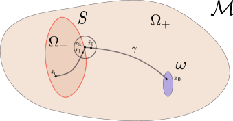
Figure 4: First step of the iteration process for the proof of Theorem 5.14. Information is propagated from $x_{0}$ to $x_{1}$. The process is then repeated starting from $x_{1}$.

Let us now look at the path joining $x_{0}$ to $\tilde{x}_{0}$. This path is entirely either in $\Omega_{+}$ or $\Omega_{-}$ and in particular one can apply the results of [LL19]. More precisely one can construct an appropriate foliation such that one can apply Theorem 4.7 of [LL19]. The construction is exactly as in the proof of Theorem 6.3 in [LL19]. The difference is that here we only use the foliation to apply Theorem 4.7 which solely concerns low frequency information. That is because in our case, this is only the first step of the propagation. Indeed, since we will need to continue the iteration we can not consider high frequencies yet.

Applying Theorem 4.7 of [LL19] gives us a set $U\subset\mathbb{R}_{t}\times\Omega_{+}$ such that

$$U\vartriangleleft[-T,T]\times\tilde{\omega},$$

and the precise construction of [LL19, Proof of theorem 6.3] implies that $U$ contains a set of the form

$$[-T_{0},T_{0}]\times\left(\{\phi_{S,1}>\frac{\rho}{2}\}\cap B(x_{S,1},r_{S,1}),4R)\right)\Subset U.$$ (5.18)

The time $T_{0}$ is equal to $T_{0}=T-\tilde{T}_{0}$ where $\tilde{T}_{0}$ is the time given by [LL19] to propagate the information from $x_{0}$ to $\tilde{x}_{0}$. This is any time greater than the length of the path joining those two points.

We can now apply Lemma 5.15 which ensures that for arbitrary $\epsilon>0$ there exists $r_{\epsilon}$ with

$$[-T_{0}+2\epsilon,T_{0}-2\epsilon]\times B(x_{S_{1}},r_{\epsilon})\vartriangleleft U.$$

Since by construction of $U$ we have $U\vartriangleleft[-T,T]\times\tilde{\omega}$, using once again the transitivity of $\vartriangleleft$ we have finally shown that

$$[-T_{0}+2\epsilon,T_{0}-2\epsilon]\times B(x_{S,1},r_{\epsilon})\vartriangleleft[-T,T]\times\tilde{\omega}.$$

Recalling that $x_{S,1}\in S$ the above property says that we managed to pass on (a possibly very small) neighborhood of the other side of the interface, and this by losing an arbitrarily small time. In particular we have shown that we can find a $x_{1}\in\gamma\left(\gamma^{-1}(x_{S,1}),1]\right)$ such that

$$[-T_{0}+2\epsilon,T_{0}-2\epsilon]\times V(x_{1})\vartriangleleft[-T,T]\times\tilde{\omega},$$ (5.19)

where $V(x_{1})$ is a (small) neighborhood of $x_{1}$. We can now repeat this propagation procedure starting from the point $x_{1}$. We consider a point $\tilde{x}_{1}$ which is on the same side of the interface as $x_{1}$, that is $\tilde{x}_{1}\in\gamma\left((\gamma^{-1}(x_{S,1}),\gamma^{-1}(x_{S,2}))\right)$ and sufficiently close to the interface and we propagate the information from $x_{1}$ to $\tilde{x}_{1}$ using Theorem 4.7 of [LL19]. Then we pass on the other side of the interface using Lemma 5.15. Iterating this process $N$ times and using the transitivity of $\vartriangleleft$ gives

$$[-T_{N}+2N\epsilon,T_{N}-2N\epsilon]\times V(y_{0})\vartriangleleft[-T,T]\times\tilde{\omega},$$

with $T_{N}=T-\sum_{0\leq j\leq N}\tilde{T}_{j}$ and $\tilde{T}_{j}$ any number strictly larger than the length of the path joining $x_{j}$ to $\tilde{x}_{j}$. Notice that the definition of $\mathcal{L}(\mathcal{M},\tilde{\omega})$ (see (1.5)) implies thanks to our assumption $T>\mathcal{L}(\mathcal{M},\tilde{\omega})$ that $T_{N}>0$ and since $\epsilon$ can be chosen arbitrarily small we can have

$$\eta_{y_{0}}:=T_{N}-2N\epsilon>0.$$

Figure 5: The iteration process of the proof of Theorem 5.14 in space-time. We transport information from a point $x_{0}\in\omega$ to $y_{0}\in\mathcal{M}$ by following the path $\gamma$. The points $x_{S,j}$ are the intersection points of $\gamma$ with $S$. The green arrows correspond to propagation of information in the smooth context where we use the results of [LL19]. The orange arrows propagate the information through the interface using Theorem 5.1 and this, by losing an arbitrarily small time.

To sum up, for an arbitrary $y_{0}\in\mathcal{M}$ we were able to find an $\eta_{y_{0}}>0$ and a neighborhood $V(y_{0})$ of $y_{0}$ such that

$$[-\eta_{y_{0}},\eta_{y_{0}}]\times V(y_{0})\vartriangleleft[-T,T]\times\tilde{\omega}.$$ (5.20)

We have thus completed the iteration procedure.

Step 2: Unfolding the definition of $\vartriangleleft$

The last part of the proof will be to write down the definition of $\vartriangleleft$ and obtain the desired estimate using a compactness argument for $\mathcal{M}$.

Define $U_{y_{0}}$ as

$$U_{y_{0}}:=[-\eta_{y_{0}},\eta_{y_{0}}]\times V(y_{0}).$$

Consider a sufficiently small neighborhood $\tilde{V}(y_{0})$ of $y_{0}$ such that $K\Subset U_{y_{0}}$, where we define $K$ as

$$K:=\left[-\frac{\eta_{y_{0}}}{2},\frac{\eta_{y_{0}}}{2}\right]\times\tilde{V}(y_{0}).$$

Pick $\chi\in C^{\infty}_{0}(U_{y_{0}})$ such that $\chi=1$ on a neighborhood $U_{\chi}$ of $K$ and $\phi\in C^{\infty}_{0}((-T,T)\times\omega)$ with $\phi=1$ on a neighborhood of $\tilde{\omega}$. The definition of $\vartriangleleft$ and (5.20) imply that for any $\kappa>0$, there exist $C,\beta,\kappa^{\prime},\mu_{0}>0$ such that for $\mu\geq\mu_{0}$ ,

$$Ce^{\kappa\mu}\left(\left\|M^{\mu}_{\mu}\phi_{\mu}u\right\|_{H^{1}}+\left\|Pu\right\|_{L^{2}(-T,T)\times\mathcal{M}}\right)+Ce^{-\kappa^{\prime}\mu}\left\|u\right\|_{H^{1}}\geq\left\|M_{\mu}^{\beta\mu}\chi_{\mu}u\right\|_{H^{1}}.$$ (5.21)

We want to use the almost localization of $\phi_{\mu}$ in order to control the left hand side of the above quantity. To do so we use Lemma B.10 which gives us

$$\left\|M^{\mu}_{\mu}\phi_{\mu}u\right\|_{H^{1}}\leq C\mu\left\|u\right\|_{L^{2}((-T,T)\times\omega)}+Ce^{-c\mu}\left\|u\right\|_{H^{1}}.$$

We want to inject the estimate above in (5.21). We need to be sure that the term $\left\|u\right\|_{H^{1}}$ will be multiplied by a negative exponential. We recall that $\kappa>0$ can be chosen arbitrarily small and we impose $\kappa<c/2$. Since $\mu\leq Ce^{\kappa\mu}$ we obtain with a new constant $c^{\prime}>0$:

$$\left\|M_{\mu}^{\beta\mu}\chi_{\mu}u\right\|_{H^{1}}\leq Ce^{2\kappa\mu}\left(\left\|u\right\|_{L^{2}((-T,T)\times\omega)}+\left\|Pu\right\|_{L^{2}(-T,T)\times\mathcal{M}}\right)+Ce^{-c^{\prime}\mu}\left\|u\right\|_{H^{1}}.$$ (5.22)

We need to exploit the almost localization of $\chi_{\mu}$ to control from below the left hand side of (5.22). We take $\tilde{\chi}\in C^{\infty}_{0}(U_{\chi})$ with $\tilde{\chi}=1$ in a neighborhood of $K$. We use Lemma B.1 to control:

$$\left\|\tilde{\chi}u\right\|_{L^{2}} \leq\left\|\tilde{\chi}\chi_{\mu}u\right\|_{L^{2}}+\left\|\tilde{\chi}(1-\chi_{\mu})u\right\|_{L^{2}}\leq C\left\|\chi_{\mu}u\right\|_{L^{2}}+Ce^{-c\mu}\left\|u\right\|_{H^{1}}$$

$$\lesssim\left\|M^{\beta\mu}_{\mu}\chi_{\mu}u\right\|_{L^{2}}+\left\|(1-M^{\beta\mu}_{\mu})\chi_{\mu}u\right\|_{L^{2}}+e^{-c\mu}\left\|u\right\|_{H^{1}}.$$ (5.23)

We control the second term as follows:

$$\left\|(1-M^{\beta\mu}_{\mu})\chi_{\mu}u\right\|_{L^{2}} =\left\|\left(1-m_{\mu}\left(\frac{\xi_{t}}{\beta\mu}\right)\right)\widehat{\chi_{\mu}u}\right\|_{L^{2}}=\left\|\frac{\left(1-m_{\mu}\left(\frac{\xi_{t}}{\beta\mu}\right)\right)}{|\xi_{t}|+|\xi_{x}|}\left(|\xi_{t}|+|\xi_{x}|\right)\widehat{\chi_{\mu}u}\right\|_{L^{2}}$$

$$\lesssim\left\|\frac{\left(1-m_{\mu}\left(\frac{\xi_{t}}{\beta\mu}\right)\right)}{|\xi_{t}|+|\xi_{x}|}\right\|_{L^{\infty}}\left\|u\right\|_{H^{1}}.$$

In the region $|\xi_{t}|\geq\frac{\beta\mu}{2}$ we simply have

$$\frac{\left(1-m_{\mu}\left(\frac{\xi_{t}}{\beta\mu}\right)\right)}{|\xi_{t}|+|\xi_{x}|}\leq\frac{C}{\mu}.$$

In the region $|\xi_{t}|\leq\frac{\beta\mu}{2}$ we use the support of $m$ and Lemma B.1 to find

$$\frac{\left(1-m_{\mu}\left(\frac{\xi_{t}}{\beta\mu}\right)\right)}{|\xi_{t}|+|\xi_{x}|}\leq Ce^{-c\mu},$$

hence in particular

$$\left\|\frac{\left(1-m_{\mu}\left(\frac{\xi_{t}}{\beta\mu}\right)\right)}{|\xi_{t}|+|\xi_{x}|}\right\|_{L^{\infty}}\leq\frac{C}{\mu}.$$

Combining estimates (5.3) and (5.22) yields:

$$\left\|\tilde{\chi}u\right\|_{L^{2}}\leq Ce^{2\kappa\mu}\left(\left\|u\right\|_{L^{2}((-T,T)\times\omega)}+\left\|Pu\right\|_{L^{2}(-T,T)\times\mathcal{M}}\right)+\frac{C}{\mu}\left\|u\right\|_{H^{1}}.$$

Since $\tilde{\chi}=1$ on $K$ we have:

$$\left\|u\right\|_{L^{2}(K)}=\left\|\tilde{\chi}u\right\|_{L^{2}(K)}\leq\left\|\tilde{\chi}u\right\|_{L^{2}}.$$

This yields, thanks to the previous estimate and the explicit definition of $K$ the final estimate:

$$\left\|u\right\|_{L^{2}\left([-\frac{\eta_{y_{0}}}{2},\frac{\eta_{y_{0}}}{2}]\times\tilde{V}(y_{0})\right)}\leq Ce^{2\kappa\mu}\left(\left\|u\right\|_{L^{2}((-T,T)\times\omega)}+\left\|Pu\right\|_{L^{2}(-T,T)\times\mathcal{M}}\right)+\frac{C}{\mu}\left\|u\right\|_{H^{1}},$$

where $\tilde{V}_{y_{0}}$ is a (small) neighborhood of $y_{0}$, $y_{0}$ is an arbitrary point of $\mathcal{M}$ and $\eta_{y_{0}}>0$ is an associated strictly positive time. One can cover the manifold $\mathcal{M}$ by such neighborhoods and by compactness we can extract a finite covering

$$\mathcal{M}\subset\bigcup_{j\in J\>\textnormal{finite}}\tilde{V}(y_{j}),$$

such that

$$\left\|u\right\|_{L^{2}\left([-\frac{\eta_{y_{j}}}{2},\frac{\eta_{y_{j}}}{2}]\times\tilde{V}(y_{j})\right)}\leq C_{j}e^{2\kappa_{j}\mu}\left(\left\|u\right\|_{L^{2}((-T,T)\times\omega)}+\left\|Pu\right\|_{L^{2}(-T,T)\times\mathcal{M}}\right)+\frac{C_{j}}{\mu}\left\|u\right\|_{H^{1}},$$

for $\mu\geq\mu_{0}$. Let $\eta:=\min\eta_{y_{j}}/2$, $C:=\max C_{j}$, $c:=\min c_{j}^{\prime}$. We have:

$$\left\|u\right\|_{L^{2}\left([-\eta,\eta]\times\mathcal{M}\right)} \leq\sum_{j\in J}\left\|u\right\|_{L^{2}\left([-\frac{\eta_{y_{j}}}{2},\frac{\eta_{y_{j}}}{2}]\times\tilde{V}(y_{j})\right)}$$

$$\leq|J|\bigg{(}Ce^{2\kappa\mu}\left(\left\|u\right\|_{L^{2}((-T,T)\times\omega)}+\left\|Pu\right\|_{L^{2}(-T,T)\times\mathcal{M}}\right)+\frac{C}{\mu}\left\|u\right\|_{H^{1}}\bigg{)}.$$

The proof of Theorem 5.14 is now complete. ∎

In the preceding theorem we chose to present a proof in the case where our observation domain $\omega$ is an open subset of $\mathcal{M}$. The point is that the difficulty of our problem comes from the interface inside $\mathcal{M}$ where the metric may jump. The Theorem and its proof show how we can propagate the information when crossing the interface in a way that is compatible with the quantitative results of [LL19]. Since in [LL19] the boundary case has been treated too, we can as well formulate the analogous result in the case of boundary observation. More precisely one has:

Theorem 5.16.

Under the assumptions of Theorem 5.14 assume additionally that $\partial\mathcal{M}$ is non empty and consider $\Gamma$ a non empty open subset of $\partial\Gamma$. Then for any $T>\mathcal{L}(\mathcal{M},\Gamma)$, there exist $\eta,C,\kappa,\mu_{0}>0$ such that for any $u\in H^{1}((-T,T)\times\mathcal{M})$ and $f\in L^{2}((-T,T)\times\mathcal{M})$ solving 5.13, we have for any $\mu\geq\mu_{0}$

$$\left\|u\right\|_{L^{2}((-\eta,\eta)\times\mathcal{M})}\leq Ce^{\kappa\mu}\left(\left\|\partial_{\nu_{\Gamma}}u\right\|_{L^{2}((-T,T)\times\Gamma)}+\left\|f\right\|_{L^{2}(-T,T)\times\mathcal{M}}\right)+\frac{C}{\mu}\left\|u\right\|_{H^{1}((-T,T)\times\mathcal{M})}.$$

One can now combine the two preceding theorems with classical energy estimates for solutions of the wave equation that allow to relate $\left\|u\right\|_{H^{1}}$ and $\left\|u\right\|_{L^{2}}$ with the energy of its initial data $(u,\partial_{t}u)_{|t=0}$ to obtain the following slightly more general version of Theorem 1.1:

Theorem 5.17.

Let $(\mathcal{M},g)$ be a smooth compact connected $n$-dimensional Riemannian manifold with (or without) boundary and $S$ an $(n-1)$-dimensional smooth submanifold of $\mathcal{M}$. We write $\mathcal{M}\backslash S=\Omega_{-}\cup\Omega_{+}$. Consider $P$ as defined in (1.2). For any nonempty open subset $\omega$ of $\mathcal{M}\backslash S$ and any $T>\mathcal{L}(\mathcal{M},\omega)$, there exist $C,\kappa,\mu_{0}$ such that for any $(u_{0},u_{1})\in H^{1}_{0}(\mathcal{M})\times L^{2}(\mathcal{M})$, $f\in L^{2}((-T,T)\times\mathcal{M})$ and $u$ solving

$$\begin{cases}Pu=f&\textnormal{in}\>(-T,T)\times\Omega_{-}\cup\Omega_{+}\\ u_{|S_{-}}=u_{|S_{+}}&\textnormal{in}\>(-T,T)\times S\\ (c\partial_{\nu}u)_{|S_{-}}=(c\partial_{\nu}u)_{|S_{+}}&\textnormal{in}\>(-T,T)\times S\\ u=0&\textnormal{in}\>(-T,T)\times\partial\mathcal{M}\\ \left(u,\partial_{t}u\right)_{|t=0}=(u_{0},u_{1})&\textnormal{in}\>\mathcal{M},\end{cases}$$ (5.24)

one has, for any $\mu\geq\mu_{0}$,

$$\left\|(u_{0},u_{1})\right\|_{L^{2}\times H^{-1}}\leq Ce^{\kappa\mu}\left(\left\|u\right\|_{L^{2}((-T,T)\times\omega)}+\left\|f\right\|_{L^{2}(-T,T)\times\mathcal{M}}\right)+\frac{C}{\mu}\left\|(u_{0},u_{1})\right\|_{H^{1}\times L^{2}}.$$

If moreover $\mathcal{M}\neq\emptyset$ and $\Gamma$ is a non empty open subset of $\partial\mathcal{M}$, for any $T>\mathcal{L}(\mathcal{M},\Gamma)$, there exist $C,\kappa,\mu_{0}>0$ such that for any $(u_{0},u_{1})\in H^{1}_{0}(\mathcal{M})\times L^{2}(\mathcal{M})$, $f\in L^{2}((-T,T)\times\mathcal{M})$ and $u$ solving (5.24), we have

$$\left\|(u_{0},u_{1})\right\|_{L^{2}\times H^{-1}}\leq Ce^{\kappa\mu}\left(\left\|\partial_{\nu_{\Gamma}}u\right\|_{L^{2}((-T,T)\times\Gamma)}+\left\|f\right\|_{L^{2}(-T,T)\times\mathcal{M}}\right)+\frac{C}{\mu}\left\|(u_{0},u_{1})\right\|_{H^{1}\times L^{2}}.$$

Appendix A A few facts on pseudodifferential calculus

We collect here some facts and notations concerning the symbolic calculus which is an essential ingredient for the proof of the Carleman estimate. We follow here the exposition of [LRL13] and [LRLR22, Chapter 2].

A.1 Differential operators

For $(t,x)\in\mathbb{R}_{t}\times\mathbb{R}^{n}_{x}$ we write $(t,x)=(t,x^{\prime},x_{n})$. The variable $x_{n}$ is normal to the interface. We use as well the notation $D_{x_{j}}:=\frac{1}{i}\partial_{x_{j}}$.

We denote by $\mathcal{D}^{m}_{\tau}$ the set of differential operators depending on $\tau$, that is operators of the form

$$P(t,x,D_{t},D_{x},\tau)=\sum_{j+|\alpha|\leq m}a_{j,\alpha}(t,x)\tau^{j}D_{t,x}^{\alpha}.$$

Their principal symbols are defined as

$$\sigma(P)=\sum_{j+|\alpha|=m}a_{j,\alpha}(t,x)\tau^{j}(\xi_{t}\xi)^{\alpha}.$$

The set of tangential operators depending on the large parameter $\tau$ is denoted by $\mathcal{D}^{m}_{\top,\tau}$ and contains operators of the form

$$P(t,x,D_{t},D_{x^{\prime}},\tau)=\sum_{j+|\alpha|\leq m}a_{j,\alpha}(t,x)\tau^{j}(D_{t}D_{x^{\prime}})^{\alpha}$$

with principal symbols defined as

$$\sigma(P)=\sum_{j+|\alpha|=m}a_{j,\alpha}(t,x)\tau^{j}(\xi_{t}\xi^{\prime})^{\alpha}.$$

A.2 Standard tangential classes

For $m\in\mathbb{R}$ we define the class tangential symbols $\mathcal{S}^{m}$ as the smooth functions on $\mathbb{R}^{n+1}\times\mathbb{R}^{n}$ such that for all $(\alpha,\beta)\in\mathbb{N}^{n+1}\times\mathbb{N}^{n}$,

$$\sup_{(t,x,\xi_{t},\xi^{\prime})}(1+|\xi^{\prime}|^{2}+|\xi_{t}|^{2})^{\frac{-m+|\beta|}{2}}|(\partial^{\alpha}_{t,x}\partial^{\beta}_{\xi_{t},\xi^{\prime}})a(t,x,\xi_{t},\xi^{\prime})|<\infty.$$

We shall mainly work with the Weyl quantization which associates to $a\in\mathcal{S}^{m}$ an operator denoted by $\textnormal{op}^{w}(a)$ defined by

$$(\textnormal{op}^{w}(a)u)(t,x^{\prime},x_{n}) =$$

$$(2\pi)^{-n}\iint_{\mathbb{R}^{2n}}e^{i\left((t,x^{\prime})-(s,y^{\prime})\right)\cdot(\xi_{t},\xi^{\prime})}a\left(\frac{t+s}{2},\frac{x^{\prime}+y^{\prime}}{2},x_{n},\xi^{\prime}\right)u(y^{\prime},s,x_{n})dsdy^{\prime}d\xi^{\prime}d\xi_{t}.$$

These integrals may not be defined in the classical sense (Lebesgue integration). They are however well defined as oscillatory integrals.

We denote by $\Psi^{m}$ the set of these pseudodifferential operators. We define as well

$$\mathcal{S}^{-\infty}:=\bigcap_{m\in\mathbb{R}}\mathcal{S}^{m},\quad\Psi^{-\infty}:=\bigcap_{m\in\mathbb{R}}\Psi^{m}.$$

Notice that even though the operators above are tangential we do not use any special notation since all pseudodifferential operators we consider are tangential.

A basic feature of the Weyl quantization is that we have the exact equality:

$$(\textnormal{op}^{w}(a))^{*}=\textnormal{op}^{w}(\bar{a}),$$

where we denote by ^∗ the adjoint operator on $L^{2}$. In particular, operators associated to real valued symbols are (formally) self-adjoint.

For $a\in\mathcal{S}^{m}$ we call principal symbol, $\sigma(a)$, the equivalence class of $a$ in $\mathcal{S}^{m}/\mathcal{S}^{m-1}.$

Many times we refer to the Sobolev regularity property of pseudodifferential calculus, namely:

$$\textnormal{op}^{w}(a):L^{2}(\mathbb{R}_{x_{n}};H^{s+m}(\mathbb{R}^{n}_{t,x^{\prime}}))\rightarrow L^{2}(\mathbb{R}_{x_{n}};H^{s}(\mathbb{R}^{n}_{t,x^{\prime}}))\>\textnormal{continuously},$$

where $a\in\mathcal{S}^{m}$.

Consider now $a_{1}\in\mathcal{S}^{m_{1}}$ and $a_{2}\in\mathcal{S}^{m_{2}}$. Then there exists a $c\in\mathcal{S}^{m_{1}+m_{2}}$ such that we have

$$\textnormal{op}^{w}(a_{1})\textnormal{op}^{w}(a_{2})=\textnormal{op}^{w}(c),$$

and we denote $c:=a_{1}\sharp a_{2}$ where $\sharp$ is called the Moyal product. One has, for any $N\in\mathbb{N}$ the following asymptotic formula:

$$(a_{1}\sharp a_{2})(t,x,\xi_{t},\xi)-\sum_{j<N}\left(i\omega(D_{t,x^{\prime}},D_{\xi_{t},\xi^{\prime}};D_{y^{\prime}},D_{\eta^{\prime}})\right)^{j}a_{1}(t,x,\xi_{t},\xi)a_{2}(y,\eta)|_{y=(t,x),\eta=(\xi_{t},\xi)}\in\mathcal{S}^{m_{1}+m_{2}-N},$$ (A.1)

with $\omega(a,b;c,d)=c\cdot b-a\cdot d$. This formula implies:

1. $\textnormal{op}^{w}(a_{1})\textnormal{op}^{w}(a_{2})=\textnormal{op}^{w}(a_{1}a_{2})+\textnormal{op}^{w}(r_{1}),\quad r_{1}\in\mathcal{S}^{m_{1}+m_{2}-1}.$

2. $[\textnormal{op}^{w}(a_{1}),\textnormal{op}^{w}(a_{2})]=\textnormal{op}^{w}\left(\frac{1}{i}\{a_{1},a_{2}\}\right)+\textnormal{op}^{w}(r_{3}),\quad r_{3}\in\mathcal{S}^{m_{1}+m_{2}-2}.$

A.3 Tangential classes with a large parameter

Since we want to show a Carleman estimate which involves a large parameter, the natural class in our context is that of pseudodifferential operators with a large parameter. For $\tau\geq 1$ we define

$$\lambda^{2}_{\tau}=\tau^{2}+|\xi^{\prime}|^{2}+|\xi_{t}|^{2},$$

The class denoted by $\mathcal{S}_{\tau}^{m}$ contains the functions $a\in C^{\infty}(t,x,\xi_{t},\xi^{\prime},\tau)$ satisfying for all $(\alpha,\beta)\in\mathbb{N}^{n+1}\times\mathbb{N}^{n}$:

$$\sup_{\begin{subarray}{c}(t,x,\xi_{t},\xi^{\prime})\\ \tau\geq 1\end{subarray}}\lambda_{\tau}^{-m+|\beta|}(\partial^{\alpha}_{t,x}\partial^{\beta}_{\xi_{t},\xi^{\prime}})a(t,x,\xi_{t},\xi^{\prime},\tau)|<\infty.$$

We set $\Psi^{m}_{\tau}:=\{\textnormal{op}^{w}(a),\>a\in\mathcal{S}^{m}_{\tau}\}$ and

$$\mathcal{S}^{-\infty}_{\tau}:=\bigcap_{m\in\mathbb{R}}\mathcal{S}^{m}_{\tau},\quad\Psi^{-\infty}_{\tau}:=\bigcap_{m\in\mathbb{R}}\Psi^{m}_{\tau}.$$

We denote by $(\cdot,\cdot)$ the inner product on $L^{2}(\mathbb{R}^{n+1})$ defined by $(f,g)=\int_{\mathbb{R}^{n+1}}f\bar{g}$ and by $(\cdot,\cdot)_{\pm}$ its restriction on $L^{2}(\mathbb{R}^{n+1}_{\pm})$.

We introduce the following Sobolev norms, defined in the tangential variables:

$$\left|u(x_{n},\cdot)\right|_{H^{s}}=\left|\textnormal{op}^{w}(\lambda^{s})u(x_{n},\cdot)\right|_{L^{2}(\mathbb{R}^{n})},\quad\left|u(x_{n},\cdot)\right|_{H^{s}_{\tau}}=\left|\textnormal{op}^{w}(\lambda^{s}_{\tau})u(x_{n},\cdot)\right|_{L^{2}(\mathbb{R}^{n})}.$$

The above norms define the (usual) Sobolev space $H^{s}$ and the Sobolev space including a large parameter $H^{s}_{\tau}.$ We use many times that for $s=1$ one has the equivalence

$$\left\|\cdot\right\|_{H^{1}_{\tau}}^{2}\sim\tau^{2}\left\|\cdot\right\|_{L^{2}}^{2}+\left\|\nabla\cdot\right\|_{L^{2}}^{2}.$$

All the properties listed in Section A.2 in the classical case remain valid in the context of the large parameter. In particular we have the Sobolev regularity property, for $a\in\mathcal{S}_{m}^{\tau}$:

$$\textnormal{op}^{w}(a):L^{2}(\mathbb{R}_{x_{n}};H^{s+m}_{\tau}(\mathbb{R}^{n}_{t,x^{\prime}}))\rightarrow L^{2}(\mathbb{R}_{x_{n}};H^{s}_{\tau}(\mathbb{R}^{n}_{t,x^{\prime}})),$$

continuously and uniformly in $\tau\geq 1$. This yields that for $a\in\mathcal{S}^{m}_{\tau}$ we have

$$\left|\left(\textnormal{op}^{w}(a)u,u\right)\right|\lesssim\left\|u\right\|_{L^{2}(\mathbb{R};H^{m/2}_{\tau})}^{2}.$$

Many times in the article we absorb error terms by taking $\tau$ sufficiently large. By that we invoke the following property: If $m^{\prime}>m$ then

$$\left\|\cdot\right\|_{H^{m}_{\tau}}\leq C\tau^{-(m^{\prime}-m)}\left\|\cdot\right\|_{H^{m^{\prime}}_{\tau}},$$

for $\tau\geq 1$.

The main tool to transfer some positivity properties of the symbol to some estimate for the corresponding operator is Gårding’s inequality. We shall use it in the context of operators involving a large parameter. For a proof we refer to [LRLR22, Chapter 2]. There the standard quantization is used, the same proof works however for the Weyl quantization.

Lemma A.1 (Gårding’s inequality with a large parameter).

Consider $a\in\mathcal{S}^{m}_{\tau}$ with principal symbol $a_{m}$. Suppose that there exist $C>0$ and $R>0$ such that

$$\operatorname{Re}a_{m}(t,x,\xi_{t},\xi^{\prime},\tau)\geq C\lambda^{m}_{\tau},\quad x\in\mathbb{R}^{n+1},\>(\xi_{t},\xi^{\prime})\in\mathbb{R}^{n},\>\tau\geq 1,\>|(\xi_{t},\xi^{\prime},\tau)|\geq R,$$

then there exist $C^{\prime}$ and $\tau_{0}$ such that

$$\operatorname{Re}\left(\textnormal{op}^{w}(a)u,u\right)\geq C^{\prime}\left\|u\right\|_{L^{2}(\mathbb{R};H^{m/2}_{\tau})}^{2},$$

for $u\in\mathscr{S}(\mathbb{R}^{n+1})$ and $\tau\geq\tau_{0}$.

Before stating the last lemma of this section let us recall a definition.

Definition 5.

The essential support of a symbol $\mathcal{S}^{m}_{\tau}$, denoted by $\textnormal{essupp}(a)$ is the complement of the largest open set of $\mathbb{R}^{n+1}_{t,x}\times\mathbb{R}^{n}_{\xi_{t},\xi^{\prime}}\times\{\tau\geq 1\}$ where the estimates for $\mathcal{S}^{-\infty}_{\tau}$ hold. More precisely, a point $(t_{0},x_{0},s_{0},\xi^{\prime}_{0})\in\mathbb{R}^{n+1}\times(\mathbb{R}^{n}\backslash\{0\})$ does not lie in the essential support of $a$ if there exists a neighborhood $\mathcal{U}$ of $(t_{0},x_{0})$ and a conic neighborhood $\mathcal{V}$ of $(s_{0},\xi^{\prime}_{0})$ such that for all $m\in\mathbb{R}$ and all $(\alpha,\beta)\in\mathbb{N}^{n+1}\times\mathbb{N}^{n}$ one has

$$\sup_{\begin{subarray}{c}(t,x)\in\mathcal{U},(\xi_{t},\xi^{\prime})\in\mathcal{V}\\ \tau\geq 1\end{subarray}}\lambda_{\tau}^{-m+|\beta|}(\partial^{\alpha}_{t,x}\partial^{\beta}_{\xi_{t},\xi^{\prime}})a(t,x,\xi_{t},\xi^{\prime},\tau)|<\infty.$$

Although the natural classes for us to work with are $\mathcal{S}^{m}_{\tau}$ involving the large parameter $\tau$, for technical reasons we also have to deal with symbols in $\mathcal{S}^{m}$. Since $\mathcal{S}^{m}\not\subset\mathcal{S}^{m}_{\tau}$ one has to make sure that the chosen objects belong to the appropriate spaces. The following Lemma [LRL13, Lemma A.4] will be then very useful:

Lemma A.2.

Let $m,m^{\prime}\in\mathbb{R}$, $a_{1}(t,x,\xi_{t},\xi^{\prime})\in\mathcal{S}^{m}$ and $a_{2}(t,x,\xi_{t},\xi^{\prime},\tau)\in\mathcal{S}^{m^{\prime}}_{\tau}$ such that the essential support of $a_{2}$ is contained in a region where $|(\xi_{t},\xi^{\prime})|\gtrsim\tau$. Then

$$\textnormal{op}^{w}(a_{1})\textnormal{op}^{w}(a_{2})=\textnormal{op}^{w}(b_{1}),\quad\textnormal{op}^{w}(a_{2})\textnormal{op}^{w}(a_{1})=\textnormal{op}^{w}(b_{2}),$$

with $b_{1},b_{2}\in\mathcal{S}_{\tau}^{m+m^{\prime}}$. Moreover one has the same asymptotic formula as (A.1) with the remainder in $\mathcal{S}^{m+m^{\prime}-N}_{\tau}$.

Appendix B Some lemmata used in the quantitative estimates

In this Section we collect some estimates coming essentially from [LL19] concerning the regularization and localization operators that we introduced for the quantitative estimates.

We define for a function $f\in L^{\infty}(\mathbb{R}^{n+1})$ and $\lambda>0$:

$$f_{\lambda}(t,x):=e^{-\frac{|D_{t}|^{2}}{\lambda}}f=\left(\frac{\lambda}{4\pi}\right)^{\frac{1}{2}}\int_{\mathbb{R}}f(s,x)e^{-\frac{\lambda}{4}|t-s|^{2}}ds.$$

We use many times the fact that

$$\left\|f_{\lambda}\right\|_{L^{2}}\leq\left\|e^{-\frac{|\cdot|^{2}}{\lambda}}\right\|_{L^{\infty}(\mathbb{R}_{t})}\left\|\mathcal{F}_{t}(f)(\xi_{t},x)\right\|_{L^{2}}=\left\|f\right\|_{L^{2}}.$$

Notice also that we have

$$f\geq 0\Longrightarrow f_{\lambda}\geq 0,$$

and consequently

$$f\geq g\Longrightarrow f_{\lambda}\geq g_{\lambda}.$$ (B.1)

We now recall several Lemmas from [LL19] that we use in the main part of this article.

Lemma B.1 (Lemma 2.3 in [LL19]).

For any $d>0$, there exist $C,c>0$ such that for any $f_{1},f_{2}\in L^{\infty}(\mathbb{R}^{n+1})$ such that $\textnormal{dist}(\operatorname{supp}{f_{1}},\operatorname{supp}{f_{2}})\geq d$ and all $\lambda\geq 0$, we have

$$\left\|f_{1,\lambda}f_{2}\right\|_{L^{\infty}}\leq Ce^{-c\lambda}\left\|f_{1}\right\|_{L^{\infty}}\left\|f_{2}\right\|_{L^{\infty}},\quad\left\|f_{1,\lambda}f_{2,\lambda}\right\|_{L^{\infty}}\leq Ce^{-c\lambda}\left\|f_{1}\right\|_{L^{\infty}}\left\|f_{2}\right\|_{L^{\infty}}.$$

Lemma B.2 (Lemma 2.4 in [LL19]).

Let $f_{2}\in C^{\infty}(\mathbb{R}^{n+1})$ with all derivatives bounded, and $d>0$. Then for every $k\in\mathbb{N}$, there exist $C,c>0$ such that for all $f_{1}\in H^{k}(\mathbb{R}^{n+1})$ such that $\textnormal{dist}(\operatorname{supp}{f_{1}},\operatorname{supp}{f_{2}})\geq d$ and all $\lambda\geq 0$ we have

$$\left\|f_{1,\lambda}f_{2}\right\|_{H^{k}}\leq Ce^{-c\lambda}\left\|f_{1}\right\|_{H^{k}}.$$

Lemma B.3.

Let $\psi:\mathbb{R}^{n+1}\rightarrow\mathbb{R}$ be a Lipschitz continuous function, $f_{1}\in C^{\infty}(\mathbb{R}^{n+1})$ with bounded derivatives and $f_{2}\in C^{\infty}_{0}(\mathbb{R}^{n+1})$ such that $\textnormal{dist}(\operatorname{supp}{f_{1}(\psi),\operatorname{supp}{f_{2}}})>0$. Then, for $k\in\{0,1\}$ there exist $C,c>0$ such that for all $\lambda>0$, we have

$$\left\|f_{1,\lambda}(\psi)f_{2}\right\|_{H^{k}\rightarrow H^{k}}\leq Ce^{-c\lambda}.$$

Lemma B.3 is essentially Lemma 2.5 from [LL19]. In its statement the Lemma requires for $\psi$ to be smooth. However, since we only need to control derivatives of order at most one Lipschitz regularity is sufficient.

Lemma B.4 (Lemma 2.6 in [LL19]).

Let $f_{1},f_{2}\in C^{\infty}_{0}(\mathbb{R}^{n+1})$ such that $f_{1}=1$ in a neighborhood of $\operatorname{supp}{f_{2}}$. Then there exist $C,c>0$ such that for all $\lambda>0$, and all $u\in H^{1}(\mathbb{R}^{n+1})$, we have

$$\left\|f_{2,\lambda}\partial^{\alpha}u\right\|_{L^{2}}\leq C\left\|f_{1,\lambda}u\right\|_{H^{1}}+Ce^{-c\lambda}\left\|u\right\|_{H^{1}},\quad\textnormal{for all}\>|\alpha|\leq 1.$$

We recall that the operators $M^{\mu}_{\lambda}$ have been defined in Section 5.1.

Lemma B.5 (Lemma 2.10 in [LL19]).

Let $f_{1}$ and $f_{2}$ be in $C^{\infty}$ bounded as well as their derivatives with $\textnormal{dist}(\operatorname{supp}{f_{1}},\operatorname{supp}{f_{2}})\geq d>0$. Then for any $k\in\mathbb{N}$, there exist $C,c>0$ such that for all $\mu>0$ and $\lambda>0$, we have

$$\left\|f_{1,\lambda}M^{\mu}_{\lambda}f_{2,\lambda}\right\|_{H^{k}\rightarrow H^{k}}\leq C^{-c\frac{\mu^{2}}{\lambda}}+Ce^{-c\lambda},\quad\left\|f_{1,\lambda}M^{\mu}_{\lambda}f_{2}\right\|_{H^{k}\rightarrow H^{k}}\leq C^{-c\frac{\mu^{2}}{\lambda}}+Ce^{-c\lambda}$$

Lemma B.6 (Lemma 2.11 in [LL19]).

Let $f\in C^{\infty}_{0}(\mathbb{R}^{n+1})$. Then there exist $C,c>0$ such that for all $\mu>0$, $\lambda>0$ and $u\in H^{1}(\mathbb{R}^{n+1})$, one has

$$\left\|f_{\lambda}M^{\mu}_{\lambda}u\right\|_{H^{1}}\leq\left\|f_{\lambda}M^{2\mu}_{\lambda}u\right\|_{H^{1}}+C\left(e^{-c\frac{\mu^{2}}{\lambda}}+e^{-c\lambda}\right)\left\|u\right\|_{H^{1}}.$$

Lemma B.7 (Lemma 2.13 in [LL19]).

There exists $C>0$ such that for all $D\in\mathbb{R}$, $\tilde{\chi}\in L^{\infty}(\mathbb{R})$ such that $\operatorname{supp}{\tilde{\chi}}\subset(-\infty,D],$ for all $\lambda,\tau>0$, we have

$$\left\|e^{\tau\psi}\tilde{\chi}_{\lambda}(\psi)\right\|_{L^{\infty}}\leq C\left\|\tilde{\chi}\right\|_{L^{\infty}}\langle\lambda\rangle^{1/2}e^{D\tau}e^{\frac{\tau^{2}}{\lambda}},$$

for all $\psi\in C^{0}(\mathbb{R}^{n+1};\mathbb{R}).$

Lemma B.8 (Lemma 2.14 in [LL19]).

There exist $C,c$ such that, for any $\epsilon,\tau,\lambda,\mu>0$, for any $k\in\mathbb{N}$, we have:

$$\left\|e^{-\frac{\epsilon|D_{t}|^{2}}{2\tau}}(1-M_{\mu}^{\lambda})\right\|_{H^{k}\rightarrow H^{k}}\leq e^{-\frac{\epsilon\mu^{2}}{8\tau}}+Ce^{-c\lambda}.$$

Lemma B.9.

Let $\psi$ be a locally Lipschitz continuous real valued function on $\mathbb{R}_{t}\times\mathbb{R}^{n}_{x}$, which is a quadratic polynomial in $t$, let $R_{\sigma}>0$, and $\sigma\in C^{\infty}_{0}(B(0,R_{\sigma}))$. Let $\chi\in C^{\infty}_{0}(\mathbb{R})$ with $\operatorname{supp}(\chi)\subset(-\infty,1),$ and $\tilde{\chi}\in C^{\infty}_{0}(\mathbb{R})$ such that $\tilde{\chi}=1$ on a neighborhood of $(-\infty,3/2)$, $\operatorname{supp}{\tilde{\chi}}\subset(-\infty,2)$, and set $\chi_{\delta}(s):=\chi(s/\delta),$ $\tilde{\chi}_{\delta}(s):=\tilde{\chi}(s/\delta)$. Let $f$ be bounded, compactly supported and real analytic in the variable $t$ in a neighborhood of $\overline{B}_{\mathbb{R}_{t}}(0,R_{\sigma})$ and define

$$g:=e^{\tau\psi}\chi_{\delta,\lambda}(\psi)\tilde{\chi}_{\delta}(\psi)f\sigma_{\lambda}.$$

Then one has the following estimate: for all $c,\delta>0$ there exist $c_{0},C,N>0$ such that for any $\tau,\mu\geq 1$ and $\frac{\mu}{c}\leq\lambda\leq c\mu,$ we have

$$\left\|M_{\lambda}^{\mu/2}g(1-M_{\lambda}^{\mu})\right\|_{L^{2}\rightarrow L^{2}}\leq C\tau^{N}e^{\frac{\tau^{2}}{\lambda}}e^{2\delta\tau}e^{-c_{0}\mu}.$$

Proof.

This is essentially Lemma 2.17 in [LL19]. Its proof is based upon Lemma 2.15 from [LL19] and there the assumptions on $\psi$ and $f$ are more restrictive. However, since we only need to use a version of [LL19, Lemma 2.17] for the case $k=0$ we see that the proof works as well in the less restrictive case of Lipschitz regularity for $\psi$ (our function $\psi$ remains a quadratic polynomial in $t$) and boundedness for $f$. ∎

Lemma B.9 is used Section 5.2 for the first estimates on the terms $B_{*}$. In our case $f$ will be equal to functions which will be either independent of $t$ or simply a polynomial in $t$, therefore the real analyticity property is preserved as well.

The following lemma is taken from [LL22] and allows to replace in the quantitative estimates the observation term $\left\|u\right\|_{H^{1}(\omega)}$ by the weaker $\left\|u\right\|_{L^{2}(\omega)}$. It is used in the proof of the semi-global estimate of Theorem 5.14.

Lemma B.10 (Lemma 5.2 in [LL22]).

Let $\Omega$ be a bounded set of $\mathbb{R}^{n+1}=\mathbb{R}_{t}\times\mathbb{R}^{n}_{x}$. Let $P$ be a differential operator of order $2$, defined in a neighborhood of $\Omega$, with real principal symbol and coefficients independent of the variable $t$. Suppose as well that $P$ is elliptic in $\{\xi_{t}=0\}$. Let $\omega\Subset\Omega$ and $\theta\in C^{\infty}_{0}(\omega)$. Then there exists $C>0$ such that for all $u\in C^{\infty}_{0}(\mathbb{R}^{n+1})$ and $\mu\geq 1$, we have

$$\left\|M^{\mu}_{\mu}u\right\|_{H^{1}}\leq C\mu\left\|u\right\|_{L^{2}(\omega)}+C\left\|Pu\right\|_{L^{2}(\Omega)}+Ce^{-c\mu}\left\|u\right\|_{H^{1}}.$$

References

- [AdHG17] Giovanni Alessandrini, Maarten V. de Hoop, and Romina Gaburro. Uniqueness for the electrostatic inverse boundary value problem with piecewise constant anisotropic conductivities. Inverse Problems, 33(12):125013, 24, 2017.
- [BCDCG20] Remi Buffe, Marcelo M. Cavalcanti, Valéria N. Domingos Cavalcanti, and Ludovick Gagnon. Control and exponential stability for a transmission problem of a viscoelastic wave equation. working paper or preprint, February 2020.
- [BGM21] Lucie Baudouin, Pamela Godoy, and Alberto Mercado. Carleman estimates for the wave equation in heterogeneous media with non-convex interface. working paper or preprint, April 2021.
- [BKL16] Roberta Bosi, Yaroslav Kurylev, and Matti Lassas. Stability of the unique continuation for the wave operator via Tataru inequality and applications. J. Differential Equations, 260(8):6451–6492, 2016.
- [BLR92] Claude Bardos, Gilles Lebeau, and Jeffrey Rauch. Sharp sufficient conditions for the observation, control, and stabilization of waves from the boundary. SIAM J. Control Optim., 30:1024–1065, 1992.
- [BMO07] Lucie Baudouin, Alberto Mercado, and Axel Osses. A global carleman estimate in a transmission wave equation and application to a one-measurement inverse problem. Inverse Problems, 23(1):257, 2007.
- [Cal58] Alberto Pedro Calderón. Uniqueness in the Cauchy problem for partial differential equations. Amer. J. Math., 80:16–36, 1958.
- [Car39] Torsten Carleman. Sur un problème d’unicité pour les systèmes d’équations aux dérivées partielles à deux variables indépendantes. Ark. Mat. Astr. Fys., 26B(17):1–9, 1939.
- [CdHKU19] Peter Caday, Maarten V. de Hoop, Vitaly Katsnelson, and Gunther Uhlmann. Reconstruction of piecewise smooth wave speeds using multiple scattering. Trans. Amer. Math. Soc., 372(2):1213–1235, 2019.
- [DOP02] Anna Doubova, Axel Osses, and Jean-Pierre Puel. Exact controllability to trajectories for semilinear heat equations with discontinuous diffusion coefficients. ESAIM Control Optim. Calc. Var., 8:621–661, 2002.
- [FdLKBH01] Vera M. Fernandez de Lima, Joao E. Kogler, Jocelyn Bennaton, and Wolfgang Hanke. Wave onset in central gray matter - its intrinsic optical signal and phase transitions in extracellular polymers. An. Acad. Bras. Ciênc., 73(3):1678–2690, 2001.
- [Gag18] Ludovick Gagnon. Sufficient Conditions for the Controllability of Wave Equations with a Transmission Condition at the Interface. 28 pages, 30 figures, December 2018.
- [GL20] Jeffrey Galkowski and Matthieu Léautaud. Control from an interior hypersurface. Transactions of the American Mathematical Society, 373(5):3177–3233, 2020.
- [Hör63] Lars Hörmander. Linear Partial Differential Operators. Springer-Verlag, Berlin, 1963.
- [Hör67] Lars Hörmander. Hypoelliptic second order differential equations. Acta Math., 119:147–171, 1967.
- [Hör85] Lars Hörmander. The Analysis of Linear Partial Differential Operators, volume III. Springer-Verlag, 1985. Second printing 1994.
- [Hör92] Lars Hörmander. A uniqueness theorem for second order hyperbolic differential equations. Comm. Partial Differential Equations, 17(5-6):699–714, 1992.
- [Hör94] Lars Hörmander. The analysis of linear partial differential operators. IV, volume 275 of Grundlehren der Mathematischen Wissenschaften. Springer-Verlag, Berlin, 1994. Fourier integral operators, Corrected reprint of the 1985 original.
- [Hör97] Lars Hörmander. On the uniqueness of the Cauchy problem under partial analyticity assumptions. In Geometrical optics and related topics (Cortona, 1996), volume 32 of Progr. Nonlinear Differential Equations Appl., pages 179–219. Birkhäuser Boston, Boston, MA, 1997.
- [Leb92] Gilles Lebeau. Contrôle analytique. I. Estimations a priori. Duke Math. J., 68(1):1–30, 1992.
- [Ler19] Nicolas Lerner. Carleman Inequalities: An Introduction and More, volume 353. Springer, 2019.
- [Lio88] Jacques-Louis Lions. Contrôlabilité exacte, perturbations et stabilisation de systèmes distribués. Tome 1, volume 8 of Recherches en Mathématiques Appliquées. Masson, Paris, 1988.
- [LL19] Camille Laurent and Matthieu Léautaud. Quantitative unique continuation for operators with partially analytic coefficients. Application to approximate control for waves. J. Eur. Math. Soc. (JEMS), 21(4):957–1069, 2019.
- [LL20] Camille Laurent and Matthieu Léautaud. Unique continuation and applications. Lecture notes. unpublished, http://leautaud.perso.math.cnrs.fr/files/UCPApplications.pdf, 2020.
- [LL21] Camille Laurent and Matthieu Léautaud. Logarithmic decay for linear damped hypoelliptic wave and Schrödinger equations. SIAM J. Control Optim., 59(3):1881–1902, 2021.
- [LL22] Camille Laurent and Matthieu Léautaud. Tunneling estimates and approximate controllability for hypoelliptic equations. Memoirs of the American Mathematical Society, 276(1357), 2022.
- [LR95] Gilles Lebeau and Luc Robbiano. Contrôle exact de l’équation de la chaleur. Comm. Partial Differential Equations, 20:335–356, 1995.
- [LR10] Jérôme Le Rousseau and Luc Robbiano. Carleman estimate for elliptic operators with coefficents with jumps at an interface in arbitrary dimension and application to the null controllability of linear parabolic equations. Arch. Rational Mech. Anal., 105:953–990, 2010.
- [LR11] Jérôme Le Rousseau and Luc Robbiano. Local and global Carleman estimates for parabolic operators with coefficients with jumps at interfaces. Invent. Math., 183:245–336, 2011.
- [LRL13] Jérôme Le Rousseau and Nicolas Lerner. Carleman estimates for anisotropic elliptic operators with jumps at an interface. Analysis & PDE, 6(7):1601–1648, 2013.
- [LRLR13] Jérôme Le Rousseau, Matthieu Léautaud, and Luc Robbiano. Controllability of a parabolic system with a diffuse interface. Journal of the European Mathematical Society, 15(4):1485–1574, 2013.
- [LRLR22] Jérôme Le Rousseau, Gilles Lebeau, and Luc Robbiano. Elliptic Carleman Estimates and Applications to Stabilization and Controllability, Volume I: Dirichlet Boundary Conditions on Euclidean Space. Progress in Nonlinear Differential Equations and Their Applications. Springer International Publishing, 2022.
- [MCCP17] Fanny Morin, Matthieu Chabanas, Hadrien Courtecuisse, and Yohan Payan. Biomechanical modeling of brain soft tissues for medical applications. In Biomechanics of Living Organs. Hyperelastic Constitutive Laws for Finite Element Modeling, pages 127–146. Academic Press, 2017.
- [Rob91] Luc Robbiano. Théorème d’unicité adapté au contrôle des solutions des problèmes hyperboliques. Comm. Partial Differential Equations, 16(4-5):789–800, 1991.
- [Rob95] Luc Robbiano. Fonction de coût et contrôle des solutions des équations hyperboliques. Asymptotic Anal., 10:95–115, 1995.
- [RZ98] Luc Robbiano and Claude Zuily. Uniqueness in the Cauchy problem for operators with partially holomorphic coefficients. Invent. Math., 131(3):493–539, 1998.
- [Sym83] William W. Symes. A trace theorem for solutions of the wave equation, and the remote determination of acoustic sources. Math. Methods Appl. Sci., 5(2):131–152, 1983.
- [Tat95] Daniel Tataru. Unique continuation for solutions to PDE’s; between Hörmander’s theorem and Holmgren’s theorem. Comm. Partial Differential Equations, 20(5-6):855–884, 1995.
- [Tat99] Daniel Tataru. Unique continuation for operators with partially analytic coefficients. J. Math. Pures Appl. (9), 78(5):505–521, 1999.
- [YDdH+17] Chunquan Yu, Elizabeth A. Day, Maarten V. de Hoop, Michel Campillo, and van der Hilst Robert D. Mapping mantle transition zone discontinuities beneath the central pacific with array processing of ss precursors. J. Geophys. Res., 122(12):10364–10378, 2017.