The High Precision Numerical Calculation of Stieltjes Constants. Simple and Fast Algorithm

Abstract

We present a simple but efficient method of calculating Stieltjes constants at a very high level of precision, up to about 80000 significant digits. This method is based on the hypergeometric-like expansion for the Riemann zeta function presented by one of the authors in 1997 [17]. The crucial ingredient in this method is a sequence of high-precision numerical values of the Riemann zeta function computed in equally spaced real arguments, i.e. $\zeta(1+\varepsilon),\zeta(1+2\varepsilon),\zeta(1+3\varepsilon),...$ where $\varepsilon$ is some real parameter. (Practical choice of $\varepsilon$ is described in the main text.) Such values of zeta may be readily obtained using the PARI/GP program, which is especially suitable for this.

Keywords: Riemann zeta function, Stieltjes constants, experimental mathematics, PARI/GP computer algebra system

1 Introduction: the Riemann $\zeta$ function

Fundamental formulas in number theory are seldom numerically efficient. Although deep and absolutely precise, they may even hide the most important features of involved quantities. As a prominent example we consider the celebrated zeta function $\zeta(s)$ discovered by Euler in 1737 and published in 1744 [9] as a function of real variable and meticulously investigated by Riemann in the complex domain in his famous memoir submitted in 1859 to the Prussian Academy [20]:

$$\zeta(s)={\displaystyle\sum\limits_{n=1}^{\infty}}\frac{1}{n^{s}}\qquad\operatorname{Re}(s)>1$$ (1)

This is a special case of more general class of functions called Dirichlet series. It is divergent in the most interesting area of the complex plane, i.e., in the so called critical strip $0\leq\operatorname{Re}s\leq 1$ where all complex zeros of zeta lie. However, as was shown by Riemann, the definition (1) does contain information about the zeta function on the entire complex plane but the process of analytic continuation must be used in order to reveal global behavior of this function. There is no universal procedure how to achieve this in practice and usually various ingenious tricks are required. For example, considering simply alternating version of (1) leads to another Dirichlet series which is convergent for $\operatorname{Re}s>0$ (except $s=1$), i.e. also inside the critical strip:

$$\zeta(s)=\frac{1}{1-2^{1-s}}{\displaystyle\sum\limits_{n=1}^{\infty}}\frac{(-1)^{n}}{n^{s}}\qquad\operatorname{Re}(s)>0,\quad s\neq 1$$

However, in order to obtain globally convergent representation for $\zeta$ one has to use more sophisticated techniques. We shall describe such an approach below.

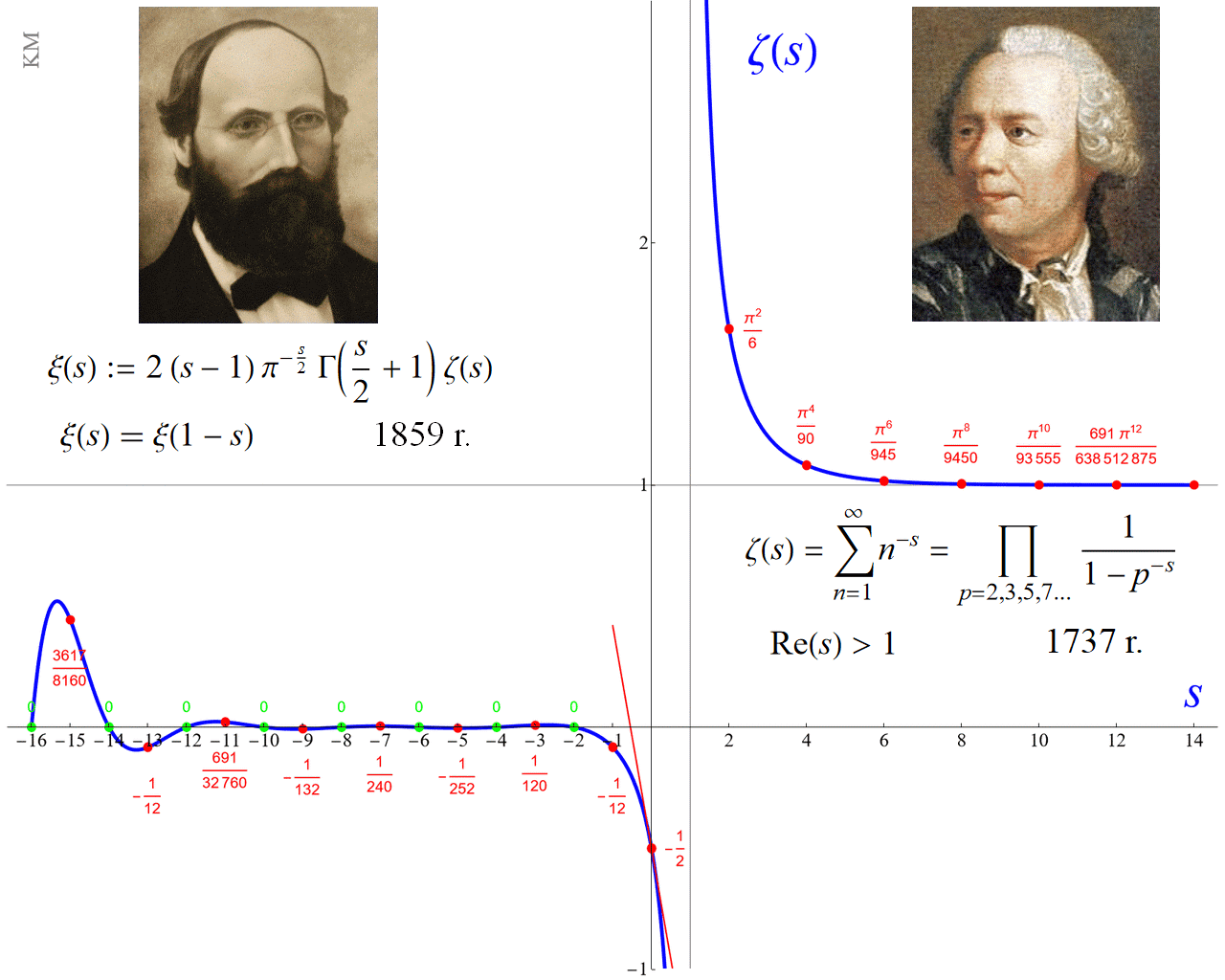
Figure 1: Plot of the zeta function for real variable (blue curve). Euler discovered the zeta function in 1737 and found its deep connection with prime numbers [9] (see box on the right). But it was Riemann who in 1859 rigorously proved certain fundamental equation for it and made its analytical continuation to the entire complex plane, except for a single pole for $s=1$ [20] (box on the left). Values of zeta for $s=2n$, $n=1,2,...$ were found by Euler in closed form (red dots). $\zeta(-2n)=0$ are so called trivial zeros (green dots).

The Riemann zeta function contains the (heavily encoded) puzzle of the distribution of prime numbers. According to the famous saying of Paul Erdös (1913-1996) – the solution to this puzzle may appear only ”in millions of years, but even then it will not be complete, because in this case we are facing Infinity”. We know, however, that this secret lies in the distribution of the zeros of the zeta function, i.e. the roots of the ”simple” equation $\zeta(s)=0$, on the complex plane. In 1859 Riemann hypothesized that all these roots (except for the so-called trivial ones) lie precisely on the line $\operatorname{Re}s=\frac{1}{2}$.

Figure 2: The zeta function shows its essence and its true meaning only in the complex domain, and we owe knowledge about it to Riemann. The upper graph is the real part of the zeta function $\zeta(s)$, the lower graph is its imaginary part in the complex domain. The blue plane is the plane of the complex variable $s$.

Figure 3: Both surfaces shown in Fig. 2 intersects the plane of the complex variable $s$ along certain irregular curves.After overlapping these surfaces, it turns out that these curves intersect themselves at certain points – these are the complex zeros of the zeta function (indicated by vertical blue lines). The Riemann hypothesis says that all these zeros are placed exactly on the line $\operatorname{Re}s=1/2$.

Despite the passage of more than a century and a half and the persistent efforts of many top-class mathematical talents, the Riemann hypothesis remains unsettled. We simply do not know whether it is true or false. (Some think that it is undecidable.) Computer experiments based on billions of numerically calculated complex roots seem to confirm it. However, exact proof remains, so far, beyond the reach of mathematicians. It seems no one has even had a good idea of how to attack this problem so far. Some have suggested that some ”new math” is needed for this, but this view is too vague to be of any practical help.

2 Stieltjes constants

The Stieltjes constants are closely related to the Riemann zeta function, and since this function is extremely important in analytical number theory, these constants are equally important.

Formulas for the Stieltjes constants may serve as another example of strict and deep but numerically inefficient formulas. These constants are essentially coefficients of the Laurent series expansion of the zeta function around its only simple pole at $s=1$:

$$\zeta(s)=\frac{1}{s-1}+{\displaystyle\sum\limits_{n=0}^{\infty}}\frac{\left(-1\right)^{n}}{n!}\gamma_{n}\left(s-1\right)^{n}$$ (2)

Primary definition of these fundamental constants was found by Thomas Jan Stieltjes and presented in a letter to his close friend and collaborator Charles Hermite dated June 23, 1885 [12]:

$$\gamma_{n}=\underset{m\rightarrow\infty}{\lim}\left({\displaystyle\sum\limits_{k=1}^{m}}\frac{\left(\ln k\right)^{n}}{k}-\frac{\left(\ln m\right)^{n+1}}{n+1}\right)$$ (3)

When $n=0$ the numerator in the first summand in (3) is formally $0^{0}$ which is taken to be $1$. In this case, (3) reduces simply to the well-known Euler-Mascheroni constant

$$\gamma_{0}=\underset{m\rightarrow\infty}{\lim}\left({\displaystyle\sum\limits_{k=1}^{m}}\frac{1}{k}-\ln m\right)$$

which, roughly speaking, measures the rate of divergence of the harmonic series.

Effective numerical computing of the constants $\gamma_{n}$ is quite a challenge because the formulas (3) are extremely slowly convergent. Even for $n=0$, in order to obtain just $10$ accurate digits one has to sum up exactly $12366$ terms whereas in order to obtain $10000$ digits (which is indeed required in some applications) one would have to sum up unrealistically large number of terms: nearly $5\cdot 10^{4342}$ which is of course far beyond capabilities of the present day computers. For $n>0$ the situation is still worse. Therefore we have to seek for other faster algorithms.

Due to the terribly slow convergence mentioned above, the progress in calculating the numerical values of Stieltjes constants values was very slow. In his letter to Hermite Stieltjes himself gave just two very inaccurate values for these constants$\gamma_{n}$ (except for the then well-known Euler-Mascheroni constant $\gamma_{0}$):

$$\gamma_{1} =-0.072815(520)...$$

$$\gamma_{2} =-0.004(7)...$$

(Here and below digits in brackets are incorrect.) Two years later, in 1887, Jensen [13] gave eight values with nine significant digits:

$$\gamma_{1} =+0.072815845...$$

$$\gamma_{2} =-0.004845182...$$

$$\gamma_{3} =-0.000342306...$$

$$\gamma_{4} =+0.0000968(89)...$$

$$\gamma_{5} =-0.000006611...$$

$$\gamma_{6} =-0.000000332...$$

$$\gamma_{7} =+0.000000105...$$

$$\gamma_{8} =-0.000000009...$$

Certain hope is in using integral representations of the Stieltjes constants. There are at least three such integrals:

– by directly applying Cauchy integral formula for derivatives to the Riemann zeta function we get:

$$\gamma_{n}=\frac{(-1)^{n}n!}{2\pi}\int_{0}^{2\pi}e^{-nit}\zeta\left(e^{it}+1\right)dt$$ (4)

– by Franel, 1895, [11]

$$\gamma_{n}=\frac{1}{2}\delta_{n,0}+\frac{1}{i}\int_{0}^{\infty}\frac{dt}{e^{2\pi t}-1}\left[\frac{\left(\ln\left(1-it\right)\right)^{n}}{1-it}-\frac{\left(\ln\left(1+it\right)\right)^{n}}{1+it}\right]$$ (5)

– by Blagouchine [6]

$$\gamma_{n}=\frac{\pi}{2(n+1)}\int_{-\infty}^{\infty}\frac{\left(\ln\left(\frac{1}{2}\pm it\right)\right)^{n+1}}{\left(\cosh\pi t\right)^{2}}dt$$ (6)

Using these integral representations one can, for exaple with the help of the procedure NIntegrate which is built in Wolfram Mathematica, calculate $\gamma_{n}$ up to $n=1000$ with precision of several hundred significant digits in a reasonable computer time. However, increasing $n$ and/or the working precision parameter in NIntegrate produces error message in the Mathematica output. This can easily be understood when looking at the behavior of the integrand of (4) which for growing $n$ contains more large oscillations.

Figure 4: Real part of the integrand (4) which contributes to the value of $\gamma_{40}$. (Integrating the imaginary part which is antisymmetric with respect to $t=\pi$ gives zero.) Number of oscillations grows as $n$. Therefore for large $n$ the numerical integration procedure cannot properly estimate this integral.

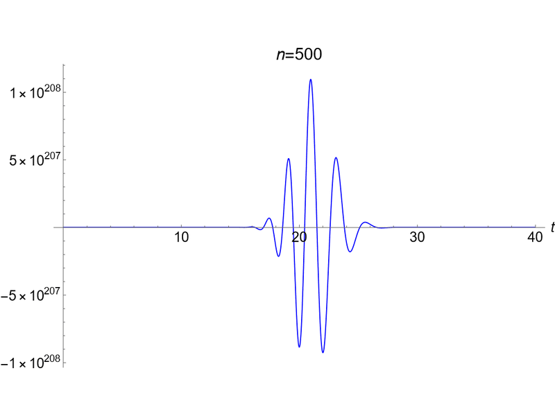
Figure 5: Real part of the integrand in (6). The number of oscillations grows with $n$ but, contrary to the case (5), their amplitude also increases very quickly with $n$.

There are also several series representations of Stieltjes constants, e.g. such as this given by I. Blagouchine [6]

$$\gamma_{n}=-\frac{1}{n+1}\sum_{k=0}^{\infty}\frac{1}{k+1}\sum_{j=0}^{\infty}(-1)^{j}\binom{k}{j}\log^{n+1}\left(j+1\right)$$ (7)

and another one found by M. Coffey [8] (Corollary 13, with misprint)

$$\gamma_{n}=-\frac{2}{3}n!\sum_{i=1}^{n}\frac{B_{n-i+1}c^{n-i}}{i!(n-i+1)!}h_{i}-\frac{2}{3c(n+1)}h_{n+1}-\frac{B_{n+1}}{n+1}c^{n+1}$$ (8)

where

$$c \equiv\ln 2$$

$$h_{i} \equiv\sum_{k=1}^{\infty}3^{-k}\sum_{j=1}^{k}\frac{(-1)^{j}2^{j}}{j+1}\binom{k}{j}\ln^{i}(j+1)$$

Unfortunately, both (7) and (8) are also very slowly convergent and pretty useless in numerical investigations – contrary to what Coffey claims: ”The expression may be attractive for some computational applications because it exhibits even faster convergence” (see [8], p. 23).

Significant progress took place in 1984-1985 with the work of Ainsworth and Howell [3] who got a grant from NASA and probably used a computer. (It could be an analog machine, but they did not disclose the technical details of their calculations.) They used another integral representation of the Stieltjes constants and with the help of the Gauss numerical integration formula tabulated $200$ initial $\gamma_{n}$ with just $10$ significant digits each. They also calculated a few selected values of $\gamma_{n}$ for larger $n=500,1000,1500,2000$. In the latter cases, some of their digits are incorrect.

In 1992 Keiper published an effective algorithm for calculating Stieltjes constants. Keiper’s algorithm was later implemented in Mathematica [15]. (However, no technical details about this algorithm can be found in Mathematica documentation except for a concise statement that it ”uses Keiper’s algorithm based on numerical quadrature of an integral representation of the zeta function and alternating series summation using Bernoulli numbers”.)

An efficient but rather complicated method based on Newton-Cotes quadrature has been proposed by Kreminski in 2003 [16]. This was a real achievement since Kreminski computed $\gamma_{n}$ up to $n=3000$ with several thousand digits and was able to observe certain interesting structures in the distribution of $\gamma_{n}$.

Quite recently (2013) Johansson presented particularly efficient method [14]. He calculated a new, impressive, record-breaking value of $\gamma_{n}$ for $n=100000$. Later (2018), in collaboration with Blagouchine, Johansson reached the next record values: $n=10^{10},10^{15}$ and $10^{100}$.

In the present paper yet another method of computing Stieltjes constants will be described which, we believe, is perhaps not as efficient as Johansson’s approach, yet it is by far more simple and it may be easily and quickly used in practical calculations for obtaining $\gamma_{n}$ up to $n\sim 30000$ with precision $\sim 80000$ significant digits.

3 Riemann zeta representation

In 1997 it was shown by one of the authors of the present paper [17], [18] that the Riemann zeta function may be expressed as

$$\zeta(s) =\frac{1}{s-1}\left[A_{0}+\left(1-\frac{s}{2}\right)A_{1}+\left(1-\frac{s}{2}\right)\left(2-\frac{s}{2}\right)\frac{A_{2}}{2!}+...\right]=$$ (9)

$$=\frac{1}{s-1}{\displaystyle\sum\limits_{k=0}^{\infty}}\frac{A_{k}}{k!}{\displaystyle\prod\limits_{i=1}^{k}}\left(i-\frac{s}{2}\right)=$$ (10)

$$=\frac{1}{s-1}{\displaystyle\sum\limits_{k=0}^{\infty}}\frac{\Gamma\left(k+1-\frac{s}{2}\right)}{\Gamma\left(1-\frac{s}{2}\right)}\frac{A_{k}}{k!}$$ (11)

$$=\frac{1}{s-1}{\displaystyle\sum\limits_{k=0}^{\infty}}\left(1-\frac{s}{2}\right)_{k}\frac{A_{k}}{k!}\qquad s\in\mathbb{C}\backslash\{1\}$$ (12)

where

$$A_{k} ={\displaystyle\sum\limits_{j=0}^{k}}\left(-1\right)^{j}\binom{k}{j}(2j+1)\zeta(2j+2)=$$ (13)

$$=\frac{1}{2}{\displaystyle\sum\limits_{j=0}^{k}}\binom{k}{j}(2j+1)\frac{\left(2\pi\right)^{2j+2}B_{2j+2}}{\left(2j+2\right)!}$$ (14)

$\left(x\right)_{k}$ is the Pochhammer symbol and $B_{n}$ is the $n^{\text{th}}$ Bernoulli number [2].

The main idea behind this approach is to remove the single pole of the zeta function multiplying it by $s-1$ and then to fix values of this entire function in an infinite number of equally spaced real points which corresponds simply to interpolation with nodes. Note that in (9)–(12) these points are precisely the points in which, as shown by Euler, zeta values are known exactly, i.e. $s=2,4,6,...$ Indeed, series (9) truncates in these points and gives appropriate exact values.

It may be shown that this representation is globally convergent. Real coefficients $A_{k}$ expressed as an alternating binomial sum are in fact combinations of Bernoulli numbers and even powers of $\pi$. On the other hand, $\left(-1\right)^{k}A_{k}$ are simply consecutive finite step derivatives of some entire function, namely $(2s+1)\zeta(2s+2)$ that involves these points in which, as Euler had shown, zeta is explicitly known.

Considered as a sort of polynomial interpolation with fixed nodes the expansion (9) might appear trivial. However, this is not the case since many ”simple” functions, e.g. Lorentz function $1/(1+x^{2})$, exhibit nasty phenomenon known as the Runge effect: oscillations between fixed nodes growing when number of terms in the series increases. This behavior may be cured using unequally spaced nodes, so called Chebyshev nodes, but this in turn spoils the very idea of (9) which leads in a natural way to Pochhammer symbols. From this point of view the global validity of (9) is equivalent to the following simple statement: the regularized Riemann zeta function $(s-1)\zeta(s)$ does not exhibit Runge phenomenon.

The original proof of (9) contained a gap [17]. Rigorous proof has been given by Báez-Duarte in 2003 [4] who also presented certain simple and esthetic criterion for the Riemann Hypothesis based on expansion (9) [5]. Another very short and particularly elegant proof of (9) using Carlson theorem has been given by Flajolet and Vepstas in 2007 [10]. Later a whole class of similar zeta representations has been published [18].

Coefficients $A_{k}$ tend to zero sufficiently fast which is crucial to assure the global convergence of the series (9). However, their detailed behavior with growing $k$ is quite striking as can be seen on a logarithmic plot with the $k$-axis rescaled as $\sqrt[3]{k}$. More precisely: they exhibit curious and unexpected oscillatory behavior with both amplitude and frequency decreasing when $k$ tends to infinity (see Fig. 6).

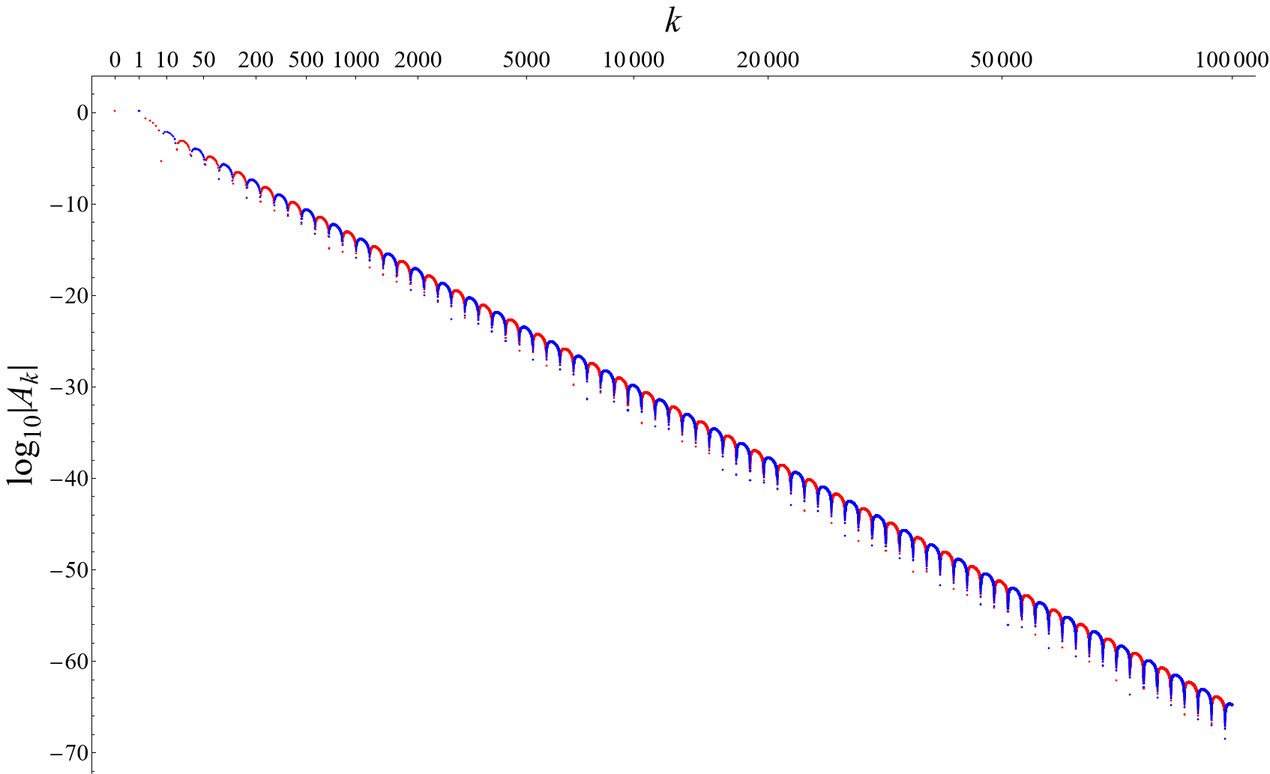
Figure 6: Curious behavior of the coefficients $A_{k}$. given by (13). There are unexpected oscillations with slowly diminishing frequency (roughly as $k^{-2/3}$) and nearly exponentially diminishing amplitude. Note that the $k$-axis is scaled as $\sqrt[3]{k}$. Red points correspond to positive values of $A_{k}$ and blue to negative ones.

This peculiar behavior ”cries for explanation” as stated in [10] (p. 2). Using the saddle point method one can show [19] that for $k$ tending to infinity the following asymptotics holds:

$$A_{k}\sim\frac{4\pi^{3/2}}{\sqrt{3\kappa}}\exp\left(-\frac{3}{2}\kappa+\frac{\pi^{2}}{4\kappa}\right)\cos\left(\frac{4\pi}{3}-\frac{3\sqrt{3}}{2}\kappa-\frac{\sqrt{3}\pi^{2}}{4\kappa}\right)$$ (15)

where

$$\kappa\equiv\pi^{3/2}\sqrt[3]{k}$$

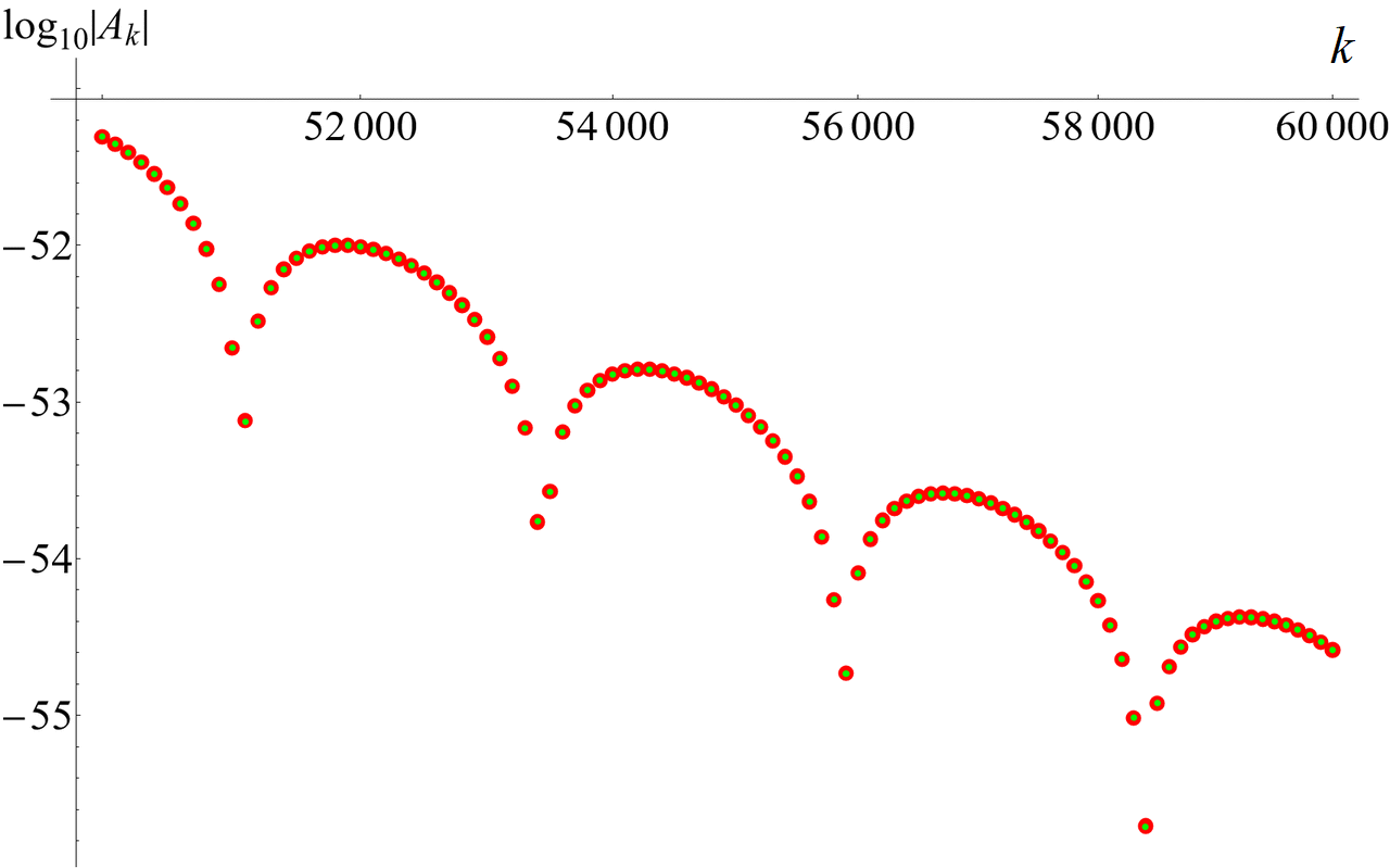
Figure 7: Asymptotic formula (15) works pretty well: red dots represent exact values of $A_{k}$ as given by (13) whereas smaller green dots are calculated from (15).

Coefficients $A_{k}$ obey also certain simple algebraic identities which stem directly from trivial zeros of zeta and from the fact that $\zeta(0)=-\frac{1}{2}$. Indeed, substituting in (9) $s=0,-2,-4,-6,...$ and making use of elementary properties of the Euler gamma function we successively get:

$${\displaystyle\sum\limits_{k=0}^{\infty}}A_{k} =\frac{1}{2}$$ (16)

$${\displaystyle\sum\limits_{k=0}^{\infty}}(k+1)A_{k} =0$$

$${\displaystyle\sum\limits_{k=0}^{\infty}}(k+1)(k+2)A_{k} =0$$

$${\displaystyle\sum\limits_{k=0}^{\infty}}(k+1)(k+2)(k+3)A_{k} =0$$

$$...$$

After some simple manipulations we finally get:

$${\displaystyle\sum\limits_{k=0}^{\infty}}k^{n}A_{k}=\frac{(-1)^{n}}{2}\qquad n=0,1,2,...$$ (17)

with the convention $k^{n}=1$ when $k=n=0$. Unfortunately, due to slow convergence of (17) when $n$ is large, these identities cannot be effectively used to calculate $A_{k}$. Another interesting identity follows from $\zeta^{\prime}(0)=-\frac{1}{2}\log(2\pi)$:

$${\displaystyle\sum\limits_{k=0}^{\infty}}A_{k}H_{k}=1-\log(2\pi)$$ (18)

where $H_{k}\equiv{\textstyle\sum\limits_{i=1}^{k}}\frac{1}{i}$ is the $k^{\text{th}}$ harmonic number.

4 Algorithm for calculating Stieltjes constants

The particular choice of nodes in $s=2,4,6,...$ in the expansion (9), albeit the most natural, is by no means the only one. One only requires that the prescribed points be strictly equally spaced. For the purpose of present calculations we choose the following sequence of points:

$$1,1+\varepsilon,1+2\varepsilon,1+3\varepsilon,...$$

where $\varepsilon$ is certain real, not necessarily small number.

More precisely, define certain entire function $f$ as:

$$f(s):=\left\{\genfrac{}{}{0.0pt}{}{\zeta(s)-\frac{1}{s-1}\qquad s\neq 1}{\gamma\qquad\qquad\qquad s=1}\right.$$ (19)

where $\gamma$ is the Euler constants which stems from the appropriate limit. Then, instead of (11), we have

$$f(s)={\displaystyle\sum\limits_{k=0}^{\infty}}\frac{\Gamma\left(k-\frac{s-1}{\varepsilon}\right)}{\Gamma\left(-\frac{s-1}{\varepsilon}\right)}\frac{\alpha_{k}}{k!}$$

with

$$\alpha_{k}={\displaystyle\sum\limits_{j=0}^{k}}\left(-1\right)^{j}\binom{k}{j}f(1+j\varepsilon)$$ (20)

Note that coefficients $\alpha_{k}$ depend on $\varepsilon$ but we shall for simplicity drop temporarily this dependence in the notation. Now directly from (2) we have:

$$\gamma_{n}=\left.(-1)^{n}\frac{d^{n}}{ds^{n}}f(s)\right|_{s-1}$$

Then, after some elementary calculations, we get the main result of the present paper:

$$\framebox{$\gamma_{n}=\frac{n!}{\varepsilon^{n}}\sum\limits_{k=n}^{\infty}\frac{(-1)^{k}}{k!}\alpha_{k}S_{k}^{(n)}$}$$ (21)

where $S_{k}^{(n)}$ are signed Stirling numbers of the first kind. Note that in the literature there are different conventions concerning denotation and indices of Stirling numbers which may be confusing. Here, following [2], we shall adopt the following convention involving the Stirling numbers and the Pochhammer symbol:

$$\left(x\right)_{k}\equiv\frac{\Gamma(k+x)}{\Gamma(x)}={\displaystyle\prod\limits_{i=0}^{k-1}}(x+i)=(-1)^{k}{\displaystyle\sum\limits_{i=0}^{k}}(-1)^{i}S_{k}^{(i)}x^{i}={\displaystyle\sum\limits_{i=0}^{k}}\left|S_{k}^{(i)}\right|x^{i}$$

Denoting

$$\beta_{nk}\equiv\frac{n!}{k!}\frac{S_{k}^{(n)}}{\varepsilon^{n}}$$

we can rewrite (21) as formally an infinite matrix product

$$\gamma_{n}={\displaystyle\sum\limits_{k=n}^{\infty}}\beta_{nk}\;\alpha_{k}$$ (22)

The summation over $k$ starts from $n$ since $\beta_{nk}\equiv 0$ for $k<n$. Precision of $\alpha_{1}$ is equal to precision of precomputed values of $f(s)$ given by (19) in equidistant nodes. When $k$ grows the precision of consecutive $\alpha_{k}$ almost linearly tends to zero. Thus there always exists certain cut-off value of $k=k_{0}$. Therefore the summation in (22) should be performed to this value:

$$\gamma_{n}={\displaystyle\sum\limits_{k=n}^{k_{0}}}\beta_{nk}\,\alpha_{k}$$ (23)

(Adding more terms is inessential. In other words, one cannot compute $\gamma_{n}$ for $n>k_{0}$. In order to perform this one should increase precision of the precomputed values of $f(s)$ which in turn would proportionally increase $k_{0}$, see Figure 9 for detailed description.)

As pointed earlier $\varepsilon$ need not to be small, however, choosing smaller $\varepsilon$ greatly accelerates convergence of the series. Yet, it turns out that smaller $\varepsilon$ implies smaller $k_{0}$. What is really important: all significant digits of $\gamma_{n}$ obtained from the finite sum (23) are correct.

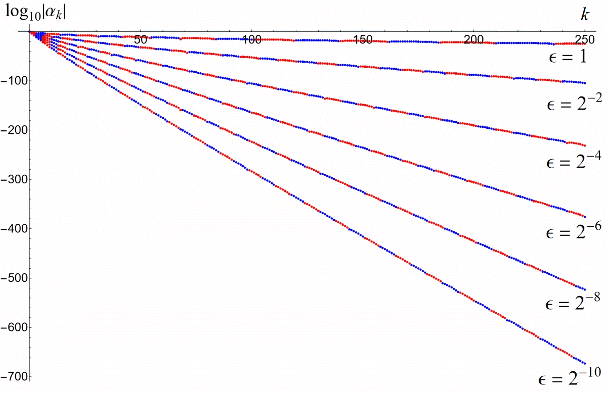
Figure 8: Behavior of coefficients $\alpha_{k}$ given by (20) for different choices of the parameter $\varepsilon$.

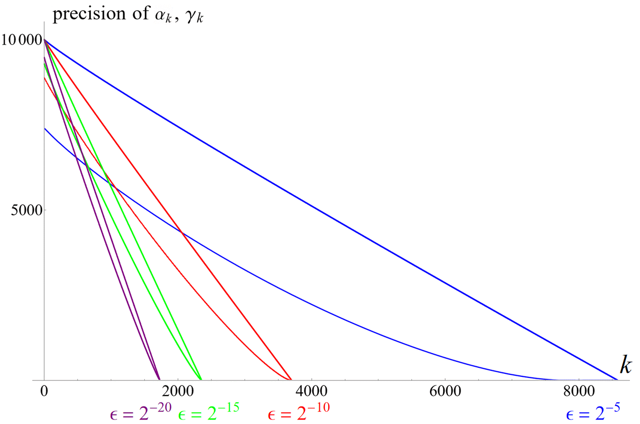
Figure 9: Plots of precision of $a_{k}$ versus $k$ for precision of the precomputed equidistant zeta values equal to 10000 significant digits and for four values of the auxiliary parameter $\varepsilon$: blue – $\varepsilon^{-5}$, red – $\varepsilon^{-10}$, green – $\varepsilon^{-15}$, purple – $\varepsilon^{-20}$. For each color the upper, nearly straight line segment corresponds to precision of $\alpha_{k}$, and piece of a curved line of the same color corresponds to the precision of $\gamma_{k}$. Since precision of $\alpha_{k}$ diminish with growing $k$ therefore for any given value of $\varepsilon$ there always exist specific, unambiguous value of index $k_{0}$ such that for all $k>k_{0}$ precisions of all $\alpha_{k}$ are numerically zero. Hence in the formula (23) it is enough to sum only up to this value.

Of course, $\gamma_{n}$ eventually does not depend on particular choice of $\varepsilon$, as expected, although $\alpha_{k}$ as well as the rate of convergence of (21)–(23) does. In fact series (21) converges for any value of $\varepsilon>0$ but the rate of convergence becomes terribly small for $\varepsilon\sim 1$. On the other hand, the smaller $\varepsilon$ the faster the rate of convergence. However, since $\alpha_{k}$ also depends on $\varepsilon$, choosing smaller value for $\varepsilon$ requires higher precision of precalculated values of $f(s)$ which in turn may be very time consuming. Hence, an appropriate compromise in choosing $\varepsilon$ is needed.

Formula (23) is particularly well-suited for numerical calculations. Typically the algorithm has three simple steps:

1. Tabulating function (19) for equidistant arguments $1+j\varepsilon$, i.e. $f(1+j\varepsilon),j=0,1,2,...$ This is most time consuming and requires appropriate choice of parameter $\varepsilon$. (In our case, we have chosen the value $\varepsilon=2^{-10}$.) The most convenient for these calculations seems small but extremely efficient program PARI/GP which has implemented particularly optimal zeta procedure. We used Cyfronet Prometheus computer where calculating single value of $f(s)$ with 80000 significant digits requires about 10-15 minutes each. Since this procedure may easily be parallelized therefore in order to compute more than 30000 values of $f$ we started several dozen independent routines (each calculating a few thousands values of $f$).

2. Calculating $\alpha_{k}$ using (20) and the precomputed values of $f$.

3. Calculating Stieltjes constants using (21).

(Contrary to the above steps 2. and 3., step 1 requires a powerful computer, whereas steps 2 and 3 can be quickly performed on a typical PC.) It should be emphasized that with the $\alpha_{k}$ coefficients properly calculated, obtaining $\gamma_{n}$ requires only a dozen or so minutes on a very modest PC machine. One property of the result (21) should again be stressed out: all digits of $\gamma_{n}$ obtained from (23) are significant and reliable.

Step 1 was achieved using the following PARI code:

$\backslash$g4

$\backslash$p 80000;

default(parisizemax, 1000000000)

allocatemem(1000000000)

eps=2^-10;

f(s) = if ( s - 1, zeta(s) - 1/(s - 1) , Euler );

for( j = 0, 32000, write( ”zeta.dat”, ”{”, 1+j*eps , ”,” , f(1+j*eps), ”},”));

5 Appendix: Struggling with certain PARI bug

Common experience shows that there are no computer programs, especially larger ones, which – in certain specific and usually unpredictable situations – would not exhibit misbehavior. Computer program errors, according to the old tradition called ”bugs”, are usually an integral part of each program. Of course, program developers, or rather the large development teams that create them, make every effort to ensure that their products are error-free. However, it is virtually impossible to remove them completely. In addition, professional computer programs are constantly developed and expanded, sometimes over many years, and new functions are added in subsequent versions, often at the explicit request of users. In this way, while previous bugs are removed, new bugs are inevitably added, although, of course, this happens unknowingly. The key role here is played by the fruitful cooperation of program users with their developers: numerous users scattered all over the world, solving their own specific problems, at the same time intensively test programs and provide their developers with relevant information about undesirable behavior of their products.

Certain sentence from a letter from PARI/GP user is particularly significant: ”I hope you and your collaborators will be able to eliminate the bugs […] in the forthcoming (final?) release of PARI” (April 1997). More than a quarter of a century has passed since then. PARI is growing, has a faithful group of users (mainly mathematicians dealing with the number theory), new functions and procedures are added, but the list of ”bugs” does not decrease at all. It is instructive to look at the page

https://pari.math.u-bordeaux.fr/cgi-bin/pkgreport.cgi?pkg=pari

illustrating the intense and fruitful interaction of PARI users with its creators. For someone unfamiliar with the essence of computer programs, the sentence from the above-quoted letter sounds like the proverbial ”wishful thinking”. It is naive and unrealistic, although it was sent in good faith. The aforementioned ”final version” of the program is an unattainable goal to which one can, at best, ”approach asymptotically”. It is also worth adding that this sentence was rightly placed on the PARI website with a meaningful title: ”Fun!”.

When testing the algorithm described in this article, we came across a surprising error in the numerical computation of the fundamental Riemann zeta function, which is built into PARI. As mentioned earlier, the presented algorithm requires ”input” zeta values of great precision; in our case, we chose $80000$ significant digits. It was a kind of compromise between relatively high precision and reasonable computation time (several weeks on many cores of the Prometheus supercomputer in Cyfronet in Kraków). Probably no one has methodically tested PARI for calculations of the Riemann zeta with such great precision before.

The choice of PARI – a small (in the command-line version only about 12 MB) dedicated to calculations in number theory as a tool to obtain the value of the zeta function – resulted from the high speed of calculations: several times greater than, for example, Mathematica (size of installation files over 4 GB). Unexpectedly tt turned out that the result file of the necessary numerical values in the form of the array $\{1+j\varepsilon,f(1+j\varepsilon)\}$ contained incorrect digits in the range of index $j$ from 11201 to 12401.

Of course, finding those digits that were wrong among more than 2.5 billion digits was quite a challenge. It was a very tedious and frustrating job, like looking for the proverbial needle in a haystack. But it was even more challenging to figure out the very cause of this error. In the first case, some properties of the $\alpha_{k}$ coefficients proved to be helpful. In the second case, professional help of the PARI program developers turned out to be indispensable.

The first sign of the presence of these erroneous digits was that the coefficients $\alpha_{k}$ calculated from these values, instead of rapidly (exponentially) decrease to zero with the increase of the index $k$, changed drastically its behavior, see Fig. 10.

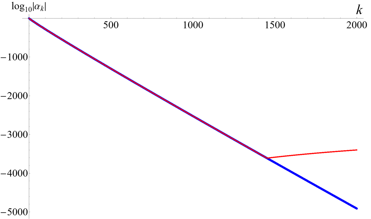
Figure 10: Coefficients $\alpha_{k}$ given by (20) are extremely sensitive to even one wrong digit in the calculated value of the zeta function, even at a very distant place of its decimal expansion. The figure illustrates a sudden change in the behavior of the $\alpha_{k}$ coefficients (red line) when in the correct value of the regularized zeta function $f(1+\varepsilon j)$ for $j=1000$ only single digit is replaced with another one that differs from the correct one just by $1$. The replaced digit might be in a very remote significant place (in this case it was on position 4000 after the decimal point), and yet $\alpha_{k}$ would ”feel” and reveal that change anyway.

Since the (regularized) zeta function, however complicated and mysterious, is a regular function, the successive finite differences of equidistant values of this function from the above-mentioned table $f(1+j\varepsilon)$ should lie on a smooth curve. The tests performed with the use of the Mathematica procedure Differences that calculates successive finite differences revealed that for the above-mentioned values of index $j$ and with the order of these differences about $400$, disturbing oscillations appeared instead of a sequence of points lying along a smooth curve, see Fig. 11.

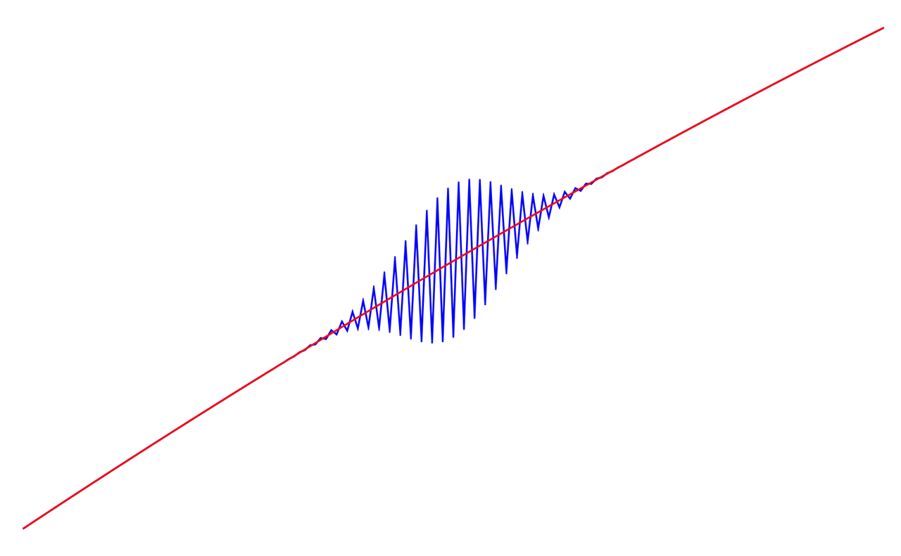
Figure 11: Wolfram Mathematica procedure Differences[list,n], which gives the $n^{\text{th}}$ differences of a given list, when applied to the list of ”contaminated” data of the function $f(1+j\varepsilon)$ reveals that some digits are wrong. When the integer parameter $n$ is sufficiently large then even a single wrong digit differing from the proper one by unity produces oscillations instead of a smooth distribution of points. In this case one had to use $n=400$ to reveal the error. (In the above graph, both axes have been removed as they are irrelevant to demonstrate the effect described.)

Intensive and very tedious tests, requiring great patience, time and computer resources, lasted for several weeks and were carried out with professional and very kind cooperation of employees of the Cyfronet Computer Center in Kraków (administrators of the Prometheus supercomputer). In order to eliminate the potential causes of generating wrong digits, we tested newer and newer development versions of PARI released daily. We used two different compilers (Intel icc 19.1.1.217 and GNU gcc version 4.8.5 20150623). We have compiled PARI in serial and parallel version (threading engine: pthread, mpi, single). Additionally, for the parallel version, we also ran single-core jobs to rule out the PARI ”parfor” command as a possible source of the problem. We used different operating systems (Linux and Windows 10), different versions of Linux cores (x86-64, x86-64 / GMP-6.2.1, x86-64 / GMP-6.0.0) and different types of processors (Intel and AMD). We compared the obtained numbers with the results obtained with Wolfram Mathematica on PCs with AMD and Intel processors (these calculations took several times longer than with PARI). We additionally performed a series of calculations for precision from 30000 to 90000 in 10000 steps and from 71000 to 89000 in 1000 steps. It turned out that the wrong numbers appeared at 174 decimal places only for the precision of 74000 and 80000.

The results of these tests were successively (from August 2021 to December 2021) delivered to the authors of the PARI program, who made appropriate corrections in the program code. (Incidentally, the first such correction did not remove the error; it appeared again but in a different range of index $j$, and even worse, i.e. for more significant digits of the Riemann zeta function…)

In the end, it turned out that the cause of this error was simply in the PARI-implemented procedure for computing the value of the zeta function which uses the classical Euler-Maclaurin algorithm. Specifically, the values of the Bernoulli numbers required to compute the zeta function were rounded unnecessarily. It was due to double roundings occurring when caching Bernoulli numbers, because of too frequent precision reductions. This bug did not affect the low precision computations, but was particularly bothersome with the algorithm described here. More details can be found here:

https://pari.math.u-bordeaux.fr/cgi-bin/bugreport.cgi?bug=2311

It should be emphasized that when computing the zeta function, PARI first computes and tabulates the appropriate Bernoulli numbers, according to the Euler-Maclaurin formula. During this stage of the calculations, which – depending on the precision set at the beginning – sometimes takes several hours, the results do not start to appear, and the program pretends that it has ”hung”.

The revised version of the program finally appeared at the end of December 2021. From that moment, having the necessary and reliable numerical data, i.e. the high precision (regularized) zeta values, we were able to return to purely mathematical problems and continue the main project of calculating the Stieltjes constants.

Finally, it should be emphasized once again that the main advantage of the presented here algorithm for calculating important Stieltjes constants is its mathematical simplicity and numerical efficiency. Moreover, it can be a convenient starting point for deriving certain new asymptotic expansion for these constants, both more accurate and simpler than several expansions known in the literature. This will be the topic of another publication [19].

Acknowledgement 1

This research was supported in part by PL-Grid Infrastructure and was performed on the Prometheus multicore supercomputer, Cyfronet, Kraków. The kind and patient willingness to help and professional technical advice from the members of the Cyfronet team (Maciej Czuchry and Andrzej Dorobisz from High Performance Computing Software Department) when starting the project were very helpful. Finally, the authors of the Pari/GP computer algebra system (Bill Allombert and Karim Belabas) put a lot of effort into correcting the persistent error in the calculation of the Riemann zeta function for the great accuracies that were crucial to the presented algorithm.

References

- [1] PARI/GP version 2.14.0, 64-bit, 2022, available from https://pari.math.u-bordeaux.fr/download.html
- [2] Milton Abramowitz, Irene A. Stegun (Eds.), Handbook of Mathematical Functions with Formulas, Graphs, and Mathematical Tables, 9th printing. New York: Dover, 1972.
- [3] O. R. Ainsworth, L. W. Howell, The Generalized Euler-Mascheroni Constants, NASA Technical Paper 2264, 1984; O. R. Ainsworth, L. W. Howell, An Integral Representation of the Generalized Euler-Mascheroni Constants, NASA Technical Paper 2456, 1985.
- [4] Luis Baez-Duarte, On Maslanka’s Representation for the Riemann Zeta Function, International Journal of Mathematics and Mathematical Sciences Volume 2010, Article ID 714147, 9 pages doi:10.1155/2010/714147.
- [5] Luis Báez Duarte, A New Necessary and Sufficient Condition for the Riemann Hypothesis, arXiv:math/0307215v1 [math.NT], 2003.
- [6] Iaroslav V. Blagouchine, A theorem for the closed-form evaluation of the first generalized Stieltjes constant at rational arguments and some related summations, arXiv:1401.3724v3 [math.NT]; Expansions of generalized Euler’s constants into the series of polynomials in and into the formal enveloping series with rational coefficients only, arXiv:1501.00740v4 [math.NT], 2016.
- [7] Iaroslav V. Blagouchine, Fredrik Johansson, Computing Stieltjes Constants Using Complex Integration, arXiv:1804.01679v3 [math.CA], 2018.
- [8] Mark Coffey, The Stieltjes constants, their relation to the coefficients, and representation of the Hurwitz zeta function,arXiv:0706.0343v2 [math-ph], 2009.
- [9] Leonhard Euler. Variae observationes circa series infinitas. Commentarii academiae scientiarum Petropolitanae, 9:160–188, 1744.
- [10] Philippe Flajolet and Linas Vepstas, On Differences of Zeta Values, arXiv:math.CA/0611332 v1 11 Nov 2006.
- [11] Jérôme Franel, (Short untitled announcement communicated by Ernesto Cesàro), L’Intermédiaire des mathematiciens. ser.1 v.2 1895, p. 153-154.
- [12] Charles Hermite and Thomas Jan Stieltjes. Correspondance d’Hermite et de Stieltjes. vol. 1, (8 novembre 1882 - 22 juillet 1889), 1905.
- [13] Johan L. W. V. Jensen, Sur la fonction de Riemann, Comptes rendus hebdomadaires des séances de l’Académie des sciences, p. 1156.
- [14] Fredrik Johansson, Rigorous high-precision computation of the Hurwitz zeta function and its derivatives. Numerical Algorithms, 69(2):253–270, Jul 2014.
- [15] Jerry B. Keiper. Power series expansions of Riemann’s function. Mathematics of Computation, 58(198):765–765, May 1992.
- [16] Rick Kreminski. Newton-Cotes integration for approximating Stieltjes (generalized Euler) constants. Mathematics of Computation, 72(243), Dec 2002.
- [17] Krzysztof Maślanka, The Beauty of Nothingness: Essay on the Zeta Function of Riemann, Acta Cosmologica XXIII-1, p. 13–18, 1998; A hypergeometric-like Representation of Zeta function of Riemann, arXiv:math-ph/0105007 v1 4 May 2001; see also http://functions.wolfram.com, citation index: 10.01.06.0012.01 and 10.01.17.0003.01.
- [18] Krzysztof Maślanka, Báez Duarte’s Criterion for the Riemann Hypothesis and Rice’s Integrals, arXiv:math/0603713v2 [math.NT] 1 Apr 2006.
- [19] Krzysztof Maślanka, An Asymptotic Expansion for the Stieltjes Constants, in preparation.
- [20] Bernhard Riemann. Ueber die Anzahl der Primzahlen unter einer gegebenen Grösse. Monatsberichte der Berliner Akademie, November 1859, pages 671–680, November 1859. English translation available at http://www.maths.tcd.ie/pub/HistMath/People/Riemann.
- [21] Stephen Wolfram, Jerry Keiper (1953–1995), The Mathematica Journal (Spring 1995), Vol. 5, issue 2, obituary available at https://www.stephenwolfram.com/publications/jerry-keiper/