Using second-order information in gradient sampling methods for nonsmooth optimization

Abstract

In this article, we show how second-order derivative information can be incorporated into gradient sampling methods for nonsmooth optimization. The second-order information we consider is essentially the set of coefficients of all second-order Taylor expansions of the objective in a closed ball around a given point. Based on this concept, we define a model of the objective as the maximum of these Taylor expansions. Iteratively minimizing this model (constrained to the closed ball) results in a simple descent method, for which we prove convergence to minimal points in case the objective is convex. To obtain an implementable method, we construct an approximation scheme for the second-order information based on sampling objective values, gradients and Hessian matrices at finitely many points. Using a set of test problems, we compare the resulting method to five other available solvers. Considering the number of function evaluations, the results suggest that the method we propose is superior to the standard gradient sampling method, and competitive compared to other methods.

1 Introduction

Nonsmooth optimization is concerned with optimizing functions that are not necessarily differentiable. Such objective functions arise in many different areas like mechanics [32], statistics [37] and machine learning [15]. Solution methods from smooth optimization generally fail to work in this case, since the local behavior of the objective can not be described by a (single) gradient. To overcome this issue, the gradient can be replaced by the so-called (Goldstein) $\varepsilon$-subdifferential [13], which essentially contains all (existing) gradients of the objective (and their limits) in an $\varepsilon$-ball around a given point. A descent direction can then be obtained by computing a direction that has a negative scalar product with all elements of the $\varepsilon$-subdifferential. This is the idea of the gradient sampling method [3], where the $\varepsilon$-subdifferential is approximated by randomly sampling gradients in the $\varepsilon$-ball. As a generalization of the standard gradient descent method from smooth optimization, only a linear convergence rate can be expected [20]. Since for the smooth case, there are higher-order methods like Newton’s method involving second-order derivative information, the question arises whether these methods can be generalized to the nonsmooth case in a similar fashion.

The first attempt to answer this question was already made in [30], where a model for the objective based on the maximum of second-order Taylor expansions was used. In [35, 27, 16], similar models were employed in bundle methods and their superlinear convergence was analyzed. In all of these methods, the second-order information is based on the Hessian of the objective function (in points where it exists). As an alternative approach, in [39, 5], the second-order information was introduced via second-order directional derivatives, and resulting solution methods were discussed from a theoretical point of view. Without focusing on optimization, an overview of second-order information for nonsmooth functions can be found in [36, 22, 33]. An approach for constructing higher-order methods that avoids the need for explicit second-order information is the direct generalization of Quasi-Newton methods to nonsmooth objective functions. This was done in [7, 8], by combining BFGS-SQP methods with gradient sampling, and in [26, 6], by directly applying smooth BFGS methods to nonsmooth problems and analyzing their behavior. (See [31] for a more detailed historic overview of higher-order methods in nonsmooth optimization.)

In this article, we will consider a second-order model of a nonsmooth, nonconvex objective function $f:\mathbb{R}^{n}\rightarrow\mathbb{R}$ and embed it into a gradient sampling framework. To motivate our approach, note that the model of $f$ used for computing descent directions in the classical gradient sampling method can be denoted as

$$z\mapsto\max_{\xi\in\partial_{\varepsilon}f(x)}f(x)+\xi^{\top}(z-x)+\frac{1}{2}\|z-x\|_{2}^{2},$$

where $\partial_{\varepsilon}f(x)$ is the $\varepsilon$-subdifferential of $f$ in $x\in\mathbb{R}^{n}$ (and $d:=z-x$ is the resulting descent direction). Formally, the expression over which the maximum is taken in this model is similar to a second-order Taylor expansion of $f$, if we interpret the elements of the $\varepsilon$-subdifferential as gradients and the identity matrix as the Hessian of $f$ in $x$. Roughly speaking, the goal of this article is to investigate what happens when we replace this expression by a “proper” second-order model of the form

$$z\mapsto\max_{y\in B_{\varepsilon}(x)}f(y)+\nabla f(y)^{\top}(z-y)+\frac{1}{2}(z-y)^{\top}\nabla^{2}f(y)(z-y),$$ (1)

where $B_{\varepsilon}(x):=\{y\in\mathbb{R}^{n}:\|x-y\|_{2}\leq\varepsilon\}$ is the closed $\varepsilon$-ball around $x$, $\nabla f$ is the gradient and $\nabla^{2}f$ is the Hessian matrix of $f$. Here, the maximum is taken over the actual second-order Taylor expansion in all points $y\in B_{\varepsilon}(x)$. Clearly, in the above form, this model is not well-defined due to nonsmoothness of $f$. To overcome this issue, we will introduce the second-order $\varepsilon$-jet of $f$ in $x$, which is a set that contains the coefficients of all (existing) second-order Taylor expansions in $B_{\varepsilon}(x)$. Since the model (1) may not be bounded below if $f$ is nonconvex, we will employ a strategy similar to a trust-region approach to be able to use it for minimization. (This also entails that we do not have to compute a step length during our algorithm.) Furthermore, we will construct a practical approximation scheme for the $\varepsilon$-jet that approximates it using only finitely many elements (similar to [29, 12] for the $\varepsilon$-subdifferential). While we will not theoretically analyze the rate of convergence of the resulting method, numerical experiments will suggest that it is faster than first-order methods like standard gradient sampling.

Although the model (1) is similar to the ones used in [30, 35, 27, 16], our approach has several differences: Firstly, in all of these works, the quadratic term in (1) was modified to be independent of the maximum by taking a weighted sum of the Hessian matrices. This makes minimizing the model significantly easier, but also impacts its approximation quality. Secondly, except for [16], all these works only considered the case where the quadratic term is positive definite, which makes it impossible to properly capture nonconvexity of $f$. Thirdly, we use the model in a gradient sampling instead of a bundle framework, resulting in an arguably simpler method. Finally, we introduce a theoretical foundation of our model via the second-order $\varepsilon$-jet, which allows us to theoretically analyze the convergence of our method independently of any finite approximation of subdifferentials (and any previous iterates).

The rest of this article is organized as follows: In Section 2, we will introduce the basic concepts from nonsmooth optimization that we build on in this article. Section 3 will introduce the second-order $\varepsilon$-jet and the resulting model of the objective function (i.e., the well-defined version of (1)). Subsequently, in Section 4, we will first construct a theoretical solution method based on this model and show convergence to minimal points of $f$ for the case where $f$ is convex (and briefly discuss convergence in the nonconvex case). Afterwards, we will construct a deterministic approximation scheme for the $\varepsilon$-jet that allows us to avoid random sampling, turning the theoretical method into a practical method. Assuming that the approximation scheme terminates, we will also show convergence of the practical method. In Section 5, we will compare a MATLAB implementation of our method to five other common methods for nonsmooth optimization in terms of performance. Finally, in Section 6, we will give a conclusion and discuss future work in this area.

2 Basic concepts

In this section, we will briefly introduce the basics of nonsmooth analysis that we build on throughout this article. For a more detailed introduction, we refer to [4, 1].

Let $f:\mathbb{R}^{n}\rightarrow\mathbb{R}$ be a locally Lipschitz continuous function and let $\Omega$ be the set of points in which $f$ is not differentiable. Although $f$ may be nonsmooth, we can obtain first-order derivative information of $f$ by considering so-called subdifferentials. To this end, let $\operatorname*{conv}(\cdot)$ be the convex hull of a set.

Definition 2.1.

Let $x\in\mathbb{R}^{n}$. The set

$$\partial f(x):=\operatorname*{conv} \left(\left\{\xi\in\mathbb{R}^{n}:\exists(x^{j})_{j}\in\mathbb{R}^{n}\setminus\Omega\text{ with }\lim_{j\rightarrow\infty}x^{j}=x\text{ and }\right.\right.$$

$$\left.\left.\lim_{j\rightarrow\infty}\nabla f(x^{j})=\xi\right\}\right)$$

is the Clarke subdifferential of $f$ in $x$. An element $\xi\in\partial f(x)$ is a Clarke subgradient.

In [4] it was shown that the Clarke subdifferential is nonempty, compact and upper semicontinuous (as a set-valued map $x\mapsto\partial f(x)$). Furthermore, the set of nondifferentiable points $\Omega$ in Definition 2.1 can be replaced by any superset of $\Omega$ with Lebesgue measure $0$ without affecting $\partial f(x)$. If $0\in\partial f(x)$ then $x$ is called a critical point of $f$, which is a necessary condition for local optimality.

Although it is possible to derive algorithms for minimizing $f$ based on the Clarke subdifferential, its usefulness in practice is hindered by its instability: Since $\partial f(x)$ reduces to $\{\nabla f(x)\}$ whenever $f$ is continuously differentiable in $x$, $\partial f(x)$ can only be used to obtain nonsmooth information in points where $f$ is not continuously differentiable, which is typically a null set (cf. Rademacher’s theorem [11]). On top of that, computing elements of $\partial f(x)$ in practice is impossible in the general case, since its definition is based on limits.

A more “stable” subdifferential was introduced in [13]. For a set $A\subseteq\mathbb{R}^{n}$ let $\overline{A}$ denote the closure of $A$ in $\mathbb{R}^{n}$.

Definition 2.2.

Let $x\in\mathbb{R}^{n}$ and $\varepsilon\geq 0$. The set

$$\partial_{\varepsilon}f(x):=\operatorname*{conv}\left(\bigcap_{\delta>\varepsilon}\overline{\{\nabla f(y):y\in B_{\delta}(x)\setminus\Omega\}}\right)$$

is the (Goldstein) $\varepsilon$-subdifferential of $f$ in $x$.

In [13] it was shown that $\partial_{\varepsilon}f(x)$ is compact and that $\partial_{0}f(x)=\partial f(x)$. More generally, the $\varepsilon$-subdifferential can be expressed in terms of the Clarke subdifferential via the equation

$$\partial_{\varepsilon}f(x)=\operatorname*{conv}(\partial f(B_{\varepsilon}(x)))$$ (2)

(see also [25], Eq. (2.1)). Roughly speaking, the $\varepsilon$-subdifferential is more stable than the Clarke subdifferential in the sense that for the $\varepsilon$-subdifferential $\partial_{\varepsilon}f(x)$, it is sufficient for $x$ to have a distance of at most $\varepsilon$ from $\Omega$ for $\partial_{\varepsilon}f(x)$ to capture the nonsmoothness of $f$. Furthermore, by definition, elements of $\partial_{\varepsilon}f(x)$ can be computed by simply evaluating (or “sampling”) the classical gradient of $f$ in different points in $B_{\varepsilon}(x)$. The drawback is that the nonsmooth information from the $\varepsilon$-subdifferential is more “blurry” than the one from the Clarke subdifferential, which makes it less accurate when used in optimality conditions (see, e.g., [1], Chapter 4).

3 Second-order information and the corresponding model for nonsmooth, nonconvex functions

In this section, we will introduce the second-order information and the corresponding model that our algorithm is based on. We will begin by discussing the class of functions to which our approach is applicable.

Let $f:\mathbb{R}^{n}\rightarrow\mathbb{R}$ and let $D^{2}\subseteq\mathbb{R}^{n}$ be the set of points in which $f$ is twice differentiable. Since our approach is based on evaluating the Hessian matrix of $f$ in different points to obtain second-order information, we restrict ourselves to cases where $\mathbb{R}^{n}\setminus D^{2}$ is a null set (implying that $D^{2}$ is dense in $\mathbb{R}^{n}$). Furthermore, since we also require first-order information of $f$, we assume that $f$ is locally Lipschitz continuous, such that we have access to the well-known concepts and results of Section 2. Although the assumptions so far already make it reasonable to sample the Hessian matrix, we need an additional assumption to obtain “boundedness”. To this end, we assume that

$$\forall x\in\mathbb{R}^{n}\exists U\subseteq\mathbb{R}^{n}\text{ open},x\in U:\{\nabla^{2}f(y):y\in U\cap D^{2}\}\text{ is bounded}.$$ (3)

(In case of first-order information, such an assumption is not required since the boundedness of the gradient follows from the local Lipschitz continuity of $f$.)

The previous assumptions allow us to properly define what we mean by “second-order information” of $f$. The idea is to replace the gradient $\nabla f(y)$ in Definition 2.2 by the coefficients of all second-order Taylor expansions of $f$, i.e., by the $4$-tuple $(y,f(y),\nabla f(y),\nabla^{2}f(y))$, and to omit the convex hull.

Definition 3.1.

Let $x\in\mathbb{R}^{n}$ and $\varepsilon\geq 0$. We refer to the set

$$\mathcal{J}_{\varepsilon}^{2}f(x) :=\bigcap_{\delta>\varepsilon}\overline{\{(y,f(y),\nabla f(y),\nabla^{2}f(y)):y\in B_{\delta}(x)\cap D^{2}\}}$$

$$\subseteq\mathbb{R}^{n}\times\mathbb{R}\times\mathbb{R}^{n}\times\mathbb{R}^{n\times n}$$

as the second-order $\varepsilon$-jet of $f$ at $x$.

In the following, we will analyze some of the properties of $\mathcal{J}_{\varepsilon}^{2}f(x)$. First of all, like the Clarke and the $\varepsilon$-subdifferential, we will show that it is nonempty and compact.

Lemma 3.2.

The set $\mathcal{J}_{\varepsilon}^{2}f(x)$ is nonempty and compact for all $x\in\mathbb{R}^{n}$ and $\varepsilon\geq 0$.

Proof.

We will first show that the set

$$T(\delta):=\{(y,f(y),\nabla f(y),\nabla^{2}f(y)):y\in B_{\delta}(x)\cap D^{2}\}$$

is bounded for all $\delta>\varepsilon$. Since we consider boundedness in a finite-dimensional product space, it is equivalent to boundedness of the projections on the individual factors. Clearly, $B_{\delta}(x)\cap D^{2}$ and $f(B_{\delta}(x)\cap D^{2})$ are bounded (due to continuity of $f$). Furthermore, $\{\nabla f(y):y\in B_{\delta}(x)\cap D^{2}\}$ is bounded as a subset of the compact set $\partial_{\delta}f(x)$. To see that $\{\nabla^{2}f(y):y\in B_{\delta}(x)\cap D^{2}\}$ is bounded as well, let $(U_{i})_{i\in I}$ be an open cover of $B_{\delta}(x)$ induced by (3) with corresponding upper bounds $(K_{i})_{i\in I}$. Due to compactness of $B_{\delta}(x)$ there is a finite subcover $(U_{i})_{i\in I^{\prime}\subseteq I}$. In particular, $\max_{i\in I^{\prime}}K_{i}$ is a bound for $\{\nabla^{2}f(y):y\in B_{\delta}(x)\cap D^{2}\}$.
Thus, $T(\delta)$ is bounded and $\overline{T(\delta)}$ is compact. In particular, $\overline{T(\delta)}$ is nonempty due to density of $D^{2}$. This means that $(\overline{T(\delta)})_{\delta>\varepsilon}$ is a nested family of nonempty, compact sets and by Cantor’s intersection theorem (see, e.g., Thm. 1 in [21]), the intersection $\mathcal{J}_{\varepsilon}^{2}f(x)=\bigcap_{\delta>\varepsilon}\overline{T(\delta)}$ is nonempty and compact. ∎

Furthermore, the second-order $\varepsilon$-jet is “compatible” with the $\varepsilon$-subdifferential in the following sense. Let $\operatorname*{pr}_{i}$, $i\in\{1,\dots,4\}$, be the projections of $\mathbb{R}^{n}\times\mathbb{R}\times\mathbb{R}^{n}\times\mathbb{R}^{n\times n}$ onto its factors.

Lemma 3.3.

Let $x\in\mathbb{R}^{n}$ and $\varepsilon\geq 0$. Then

$$\{(y,\varphi,\xi):\exists\mathcal{H}\in\mathbb{R}^{n\times n}\text{ with }(y,\varphi,\xi,\mathcal{H})\in\mathcal{J}_{\varepsilon}^{2}f(x)\}$$

$$=\{(y,f(y),\xi):y\in B_{\varepsilon}(x),\xi\in\partial f(y)\}.$$

In particular, it holds

1. $\operatorname*{pr}_{1}(\mathcal{J}_{\varepsilon}^{2}f(x))=B_{\varepsilon}(x)$,

2. $\operatorname*{pr}_{2}(\mathcal{J}_{\varepsilon}^{2}f(x))=f(B_{\varepsilon}(x))$,

3. $\operatorname*{conv}(\operatorname*{pr}_{3}(\mathcal{J}_{\varepsilon}^{2}f(x)))=\partial_{\varepsilon}f(x)$.

Proof.

“$\subseteq$”: Let $(y,\varphi,\xi,\mathcal{H})\in\mathcal{J}_{\varepsilon}^{2}f(x)$ and let $T(\delta)$ be defined as in the proof of Lemma 3.2. Then we can construct sequences $(J^{i})_{i}=(y^{i},\varphi^{i},\xi^{i},\mathcal{H}^{i})_{i}$ and $(\delta_{i})_{i}$ with $\delta_{i}>\varepsilon$, $\lim_{i\rightarrow\infty}\delta_{i}=\varepsilon$, $J^{i}\in T(\delta_{i})$ and

$$\lim_{i\rightarrow\infty}J^{i}=(y,\varphi,\xi,\mathcal{H}).$$

Continuity of $f$ shows that $\varphi=f(y)$. Furthermore, since $D^{2}\subseteq\mathbb{R}^{n}\setminus\Omega$, $\xi\in\partial f(y)$ follows from Definition 2.1.
“$\supseteq$”: Let $y\in B_{\varepsilon}(x)$ and $\xi\in\partial f(y)$. Then by definition of the Clarke subdifferential and since $\mathbb{R}^{n}\setminus D^{2}$ is assumed to be a null set, there is a sequence $(y^{i})_{i}\in D^{2}$ with $\lim_{i\rightarrow\infty}y^{i}=y$ and $\lim_{i\rightarrow\infty}\nabla f(y^{i})=\xi$. Let $J^{i}:=(y^{i},f(y^{i}),\nabla f(y^{i}),\nabla^{2}f(y^{i}))$ for $i\in\mathbb{N}$. Then there is some $\varepsilon_{0}>\varepsilon$ such that $J_{i}\in\mathcal{J}^{2}_{\varepsilon_{0}}f(x)$ for all $i\in\mathbb{N}$. Since $\mathcal{J}^{2}_{\varepsilon_{0}}f(x)$ is compact by Lemma 3.2, there is a subsequence $(i_{j})_{j}$ and a matrix $\mathcal{H}\in\mathbb{R}^{n\times n}$ such that $\lim_{j\rightarrow\infty}J^{i_{j}}=(y,f(y),\xi,\mathcal{H})=:\bar{J}$. By construction it holds $\bar{J}\in\overline{T(\delta)}$ for all $\delta>\varepsilon$, so $\bar{J}\in\mathcal{J}_{\varepsilon}^{2}f(x)$.
Finally, for (i) and (ii) note that the Clarke subdifferential is always nonempty and for (iii) recall (2). ∎

Having established some basic properties of the second-order $\varepsilon$-jet, we will now use it to construct a model function for $f$. To this end, let

$$q_{\mathcal{H}}(v):=v^{\top}\mathcal{H}v$$

be the quadratic form induced by a symmetric matrix $\mathcal{H}\in\mathbb{R}^{n\times n}$. The idea is to assign to each element of $\mathcal{J}_{\varepsilon}^{2}f(x)$ a quadratic polynomial via

$$(y,\varphi,\xi,\mathcal{H})\mapsto\varphi+\xi^{\top}(z-y)+\frac{1}{2}q_{\mathcal{H}}(z-y)$$ (4)

and to then take the maximum of these polynomials over all elements of $\mathcal{J}_{\varepsilon}^{2}f(x)$. More formally, we define the model

$$\mathcal{T}_{x,\varepsilon}(z):=\max_{(y,f(y),\xi,\mathcal{H})\in\mathcal{J}_{\varepsilon}^{2}f(x)}f(y)+\xi^{\top}(z-y)+\frac{1}{2}q_{\mathcal{H}}(z-y).$$ (5)

Due to continuity of (4) (for fixed $z\in\mathbb{R}^{n}$) and compactness of $\mathcal{J}_{\varepsilon}^{2}f(x)$ (cf. Lemma 3.2), $\mathcal{T}_{x,\varepsilon}$ is well-defined. Furthermore, it is locally Lipschitz continuous as the maximum of continuously differentiable functions. The following lemma shows that $\mathcal{T}_{x,\varepsilon}$ is an overestimate of $f$ on $B_{\varepsilon}(x)$.

Lemma 3.4.

Let $x\in\mathbb{R}^{n}$ and $\varepsilon\geq 0$. Then $f(z)\leq\mathcal{T}_{x,\varepsilon}(z)$ for all $z\in B_{\varepsilon}(x)$.

Proof.

Let $z\in B_{\varepsilon}(x)$. By Lemma 3.3 there are $\xi_{z}\in\mathbb{R}^{n}$ and $\mathcal{H}_{z}\in\mathbb{R}^{n\times n}$ such that $(z,f(z),\xi_{z},\mathcal{H}_{z})\in\mathcal{J}_{\varepsilon}^{2}f(x)$. By definition of $\mathcal{T}_{x,\varepsilon}(z)$, this implies

$$\mathcal{T}_{x,\varepsilon}(z)\geq f(z)+\xi_{z}^{\top}(z-z)+\frac{1}{2}q_{\mathcal{H}_{z}}(z-z)=f(z).$$

∎

In the following, we will compare the model $\mathcal{T}_{x,\varepsilon}$ to two other classical model functions used in nonsmooth, nonconvex optimization:

1. In the gradient sampling method [3], a direction $d\in\mathbb{R}^{n}$ is computed via

   $$d:=\operatorname*{arg\,min}_{\xi\in\partial_{\varepsilon}f(x)}\|\xi\|_{2}^{2},$$

   which corresponds (via dualization [2], for $z=x+d$) to the minimization of the model

   $$z\mapsto\max_{\xi\in\partial_{\varepsilon}f(x)}f(x)+\xi^{\top}(z-x)+\frac{1}{2}\|z-x\|_{2}^{2}.$$ (6)

   In words, (6) takes the maximum of all first-order Taylor expansions of $f$ in $x$ when we consider the elements of $\partial_{\varepsilon}f(x)$ to be gradients of $f$ in $x$, and the quadratic term ensures boundedness of the solution. If $d\neq 0$, then $d$ is a descent direction for $f$ in $x$ in the sense that $\xi^{\top}d<0$ for all $\xi\in\partial_{\varepsilon}f(x)$, and $d=0$ implies that $0\in\partial_{\varepsilon}f(x)$. While the latter property is a practical way to check if the point $x$ is close to a minimum of $f$, it also shows a drawback of the model: Since $d=0$ as soon as the distance of $x$ to a minimum is less than $\varepsilon$, the model is not able to describe the behavior of $f$ around a minimum in a way that is useful for minimization.

2. In the proximal bundle method ([24], Chapter 7 or [1], Chapter 12), a direction $d\in\mathbb{R}^{n}$ is computed via minimization of the model

   $$z\mapsto\max_{\begin{subarray}{c}y\in B_{\varepsilon}(x),\\ \xi\in\partial f(y)\end{subarray}}f(x)+\xi^{\top}(z-x)-\max(\{|\alpha(y)|,\gamma\|x-y\|_{2}^{2}\})+\frac{1}{2}u\|z-x\|_{2}^{2},$$ (7)

   $$\alpha(y):=f(x)-f(y)-\xi^{\top}(x-y),$$

   for $z=x+d$ and $\gamma>0$, $u>0$. (In the actual method, the maximum in (7) is taken over all previous iterates $y^{i}\in\mathbb{R}^{n}$ (yielding the so-called bundle) rather than all $y\in B_{\varepsilon}(x)$, but the formulation we stated here allows for a better comparison.) If $f$ is convex then $\alpha(y)\geq 0$ and for $\gamma=0$, $u=1$, (7) reduces to

   $$z\mapsto\max_{y\in B_{\varepsilon}(x),\xi\in\partial f(y)}f(y)+\xi^{\top}(z-y)+\frac{1}{2}\|z-x\|_{2}^{2}.$$ (8)

   This model is similar to (6) except that here, for the Taylor expansion, an element $\xi\in\partial_{\varepsilon}f(x)$ is considered to be a gradient of $f$ in $y\in B_{\varepsilon}(x)$ with $\xi\in\partial f(y)$ (cf. (2)) rather than simply a gradient in $x$. As a result, (7) can still be used for minimizing $f$ even when the distance of $x$ to a minimum is less than $\varepsilon$.

The model $\mathcal{T}_{x,\varepsilon}$ considered in this article is similar to (8), except that we take the second-order rather than the first-order Taylor expansion of $f$ in all $y\in B_{\varepsilon}(x)$ and omit the term $\frac{1}{2}\|z-x\|_{2}^{2}$. In particular, while both (6) and (7) are convex models even when $f$ is nonconvex, $\mathcal{T}_{x,\varepsilon}$ is potentially nonconvex. The impact of this on the approximation of $f$ is shown in the following example.

Example 3.5.

Let

$$f:\mathbb{R}\rightarrow\mathbb{R},\quad x\mapsto\max(\{\sqrt{|x|},-4|x|^{2.5}+x+1\}).$$

It is easy to see that $f$ satisfies the assumptions from the beginning of this section. (Note that $f$ does not admit the value of $\sqrt{|x|}$ near $0$.) Figure 1 shows the corresponding models of the gradient sampling method (6), the proximal bundle method (7) (with $\gamma=u=1$) and the model $\mathcal{T}_{x,\varepsilon}$ (5) for $x=0.1$, $\varepsilon=0.75$ and an approximation of $B_{\varepsilon}(x)$ using $19$ equidistant sample points.

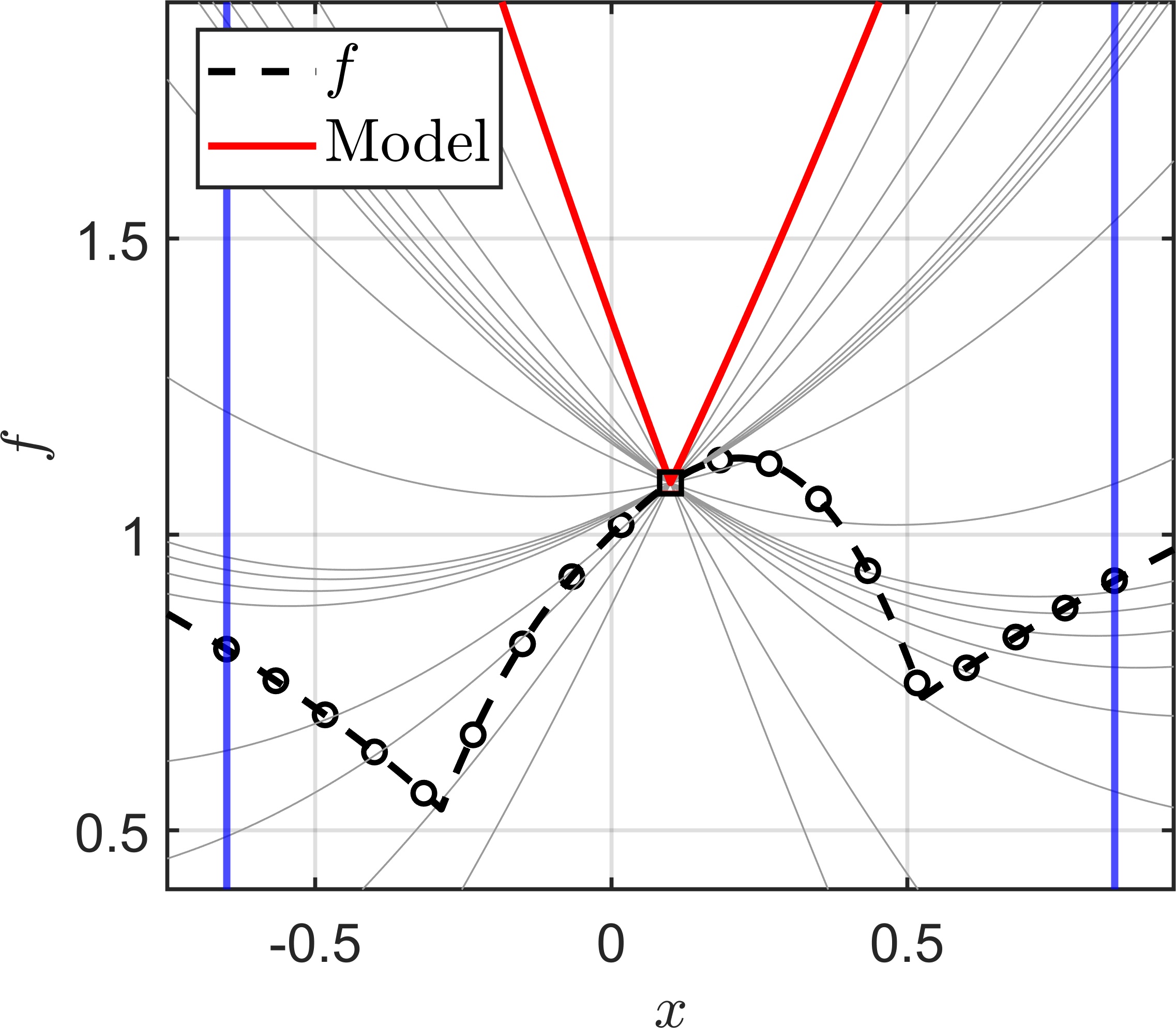
(a) Gradient sampling (6)

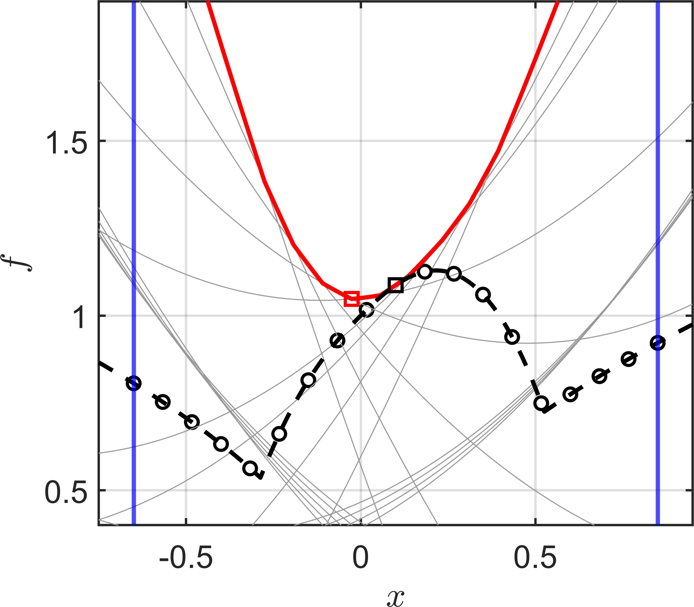
(b) Proximal bundle (7)

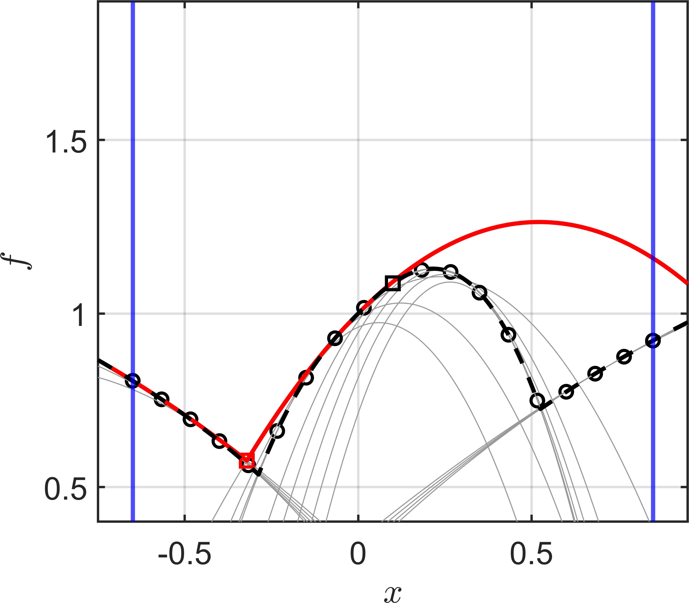
(c) $\mathcal{T}_{x,\varepsilon}$ (5)

Figure 1: Different models for $f$ in Example 3.5. The circles show the positions of the sample points, the blue lines show the boundary of $B_{\varepsilon}(x)$, the gray lines show the the individual functions over which the maximum is taken in the respective model and the red squares show the minimal points of the models (in $B_{\varepsilon}(x)$)

For the gradient sampling method in (a), we see that no descent step can be made based on the model (i.e., $d=0$). As discussed above, this is caused by $B_{\varepsilon}(x)$ containing a critical point of $f$ (or, more precisely, the global minimum, a local minimum and a local maximum of $f$ in this case). Further descent with this method can only be achieved after decreasing $\varepsilon$. In contrast to this, the proximal bundle method in (b) is still able to decrease the value of $f$, albeit the predicted decrease from the model is small considering the minimal value of $f$ in $B_{\varepsilon}(x)$. Finally, for the model $\mathcal{T}_{x,\varepsilon}$ in (c), we see that the approximation quality around the minimum of $f$ is relatively high, and the minimum of $\mathcal{T}_{x,\varepsilon}$ (constrained to $B_{\varepsilon}(x)$) is relatively close to the minimum of $f$. (Nonetheless, the approximation quality to the right of $x$ is a lot worse, showing that we can not always expect as good of a behavior of $\mathcal{T}_{x,\varepsilon}$ as in this example.)

While the previous example shows the possible advantage of using the nonconvex model $\mathcal{T}_{x,\varepsilon}$ for the minimization of $f$, it also shows the issue that the model might be unbounded below. In the following section, we will introduce a strategy for solving this issue.

4 A descent method based on the second-order model

In this section, we will construct a descent method based on minimizing the second-order model $\mathcal{T}_{x,\varepsilon}$ from the previous section. We begin by deriving a theoretical version of this method for which we assume that the whole second-order $\varepsilon$-jet $\mathcal{J}_{\varepsilon}^{2}f(x)$ is available in all $x\in\mathbb{R}^{n}$. We prove convergence to a minimum of $f$ for the case where $f$ is convex and briefly discuss convergence for the general nonconvex case. Since the assumption of being able to evaluate the whole set $\mathcal{J}_{\varepsilon}^{2}f(x)$ is too strong for the theoretical algorithm to have any practical use, we then construct a (heuristic) approximation scheme for $\mathcal{J}_{\varepsilon}^{2}f(x)$ based on only sampling single points that allows us to turn the theoretical algorithm into a practical one. Under the assumption that this approximation scheme always terminates, we show convergence of the practical method as well.

4.1 Theoretical algorithm

Since there are negative-definite matrices $\mathcal{H}\in\operatorname*{pr}_{4}(\mathcal{J}_{\varepsilon}^{2}f(x))$ when $f$ is nonconvex, the model function $\mathcal{T}_{x,\varepsilon}$ may be unbounded below. To solve this issue, we constrain $\mathcal{T}_{x,\varepsilon}$ to $B_{\varepsilon}(x)$, i.e., we consider the problem

$$\min_{z\in B_{\varepsilon}(x)}\mathcal{T}_{x,\varepsilon}(z)=\min_{z\in B_{\varepsilon}(x)}\max_{(y,f(y),\xi,\mathcal{H})\in\mathcal{J}_{\varepsilon}^{2}f(x)}f(y)+\xi^{\top}(z-y)+\frac{1}{2}q_{\mathcal{H}}(z-y).$$ (9)

This problem is well-defined since $\mathcal{T}_{x,\varepsilon}$ is continuous. Let $\theta(x,\varepsilon)\in\mathbb{R}$ be the optimal value and $\bar{z}(x,\varepsilon)\in\operatorname*{arg\,min}_{z\in B_{\varepsilon}(x)}\mathcal{T}_{x,\varepsilon}(z)$ be an arbitrary solution of (9). (For the sake of readability, we will omit the dependency of $\theta(x,\varepsilon)$ and $\bar{z}(x,\varepsilon)$ on $x$ and $\varepsilon$ whenever the context allows it.)

The idea of our method is to generate a descending sequence $(x^{i})_{i}\in\mathbb{R}^{n}$ for $f$ via $x^{i+1}=\bar{z}(x^{i},\varepsilon_{i})$ for an initial point $x^{0}\in\mathbb{R}^{n}$. For $(x^{i})_{i}$ to be a descending sequence for $f$, we have to choose $\varepsilon_{i}$ such that the model $\mathcal{T}_{x^{i},\varepsilon_{i}}$ is a “good enough” model for $f$ in $B_{\varepsilon_{i}}(x^{i})$. To this end, note that Lemma 3.4 immediately yields the following result.

Corollary 4.1.

Let $x\in\mathbb{R}^{n}$ and $\varepsilon\geq 0$. Then $f(\bar{z})\leq\theta$.

By Corollary 4.1, the difference $\theta(x^{i},\varepsilon_{i})-f(x^{i})$ can be used to estimate the descent when going from $x^{i}$ to $\bar{z}(x^{i},\varepsilon_{i})$. In particular, $\theta(x^{i},\varepsilon_{i})-f(x^{i})\geq 0$ means that descent can not be guaranteed. In this case, we will decrease $\varepsilon_{i}$ and solve (9) again. Simply assuring $\theta(x^{i},\varepsilon_{i})-f(x^{i})<0$ for the acceptance of $\bar{z}(x^{i},\varepsilon_{i})$ would be sufficient for $(x^{i})_{i}$ to be a descending sequence, but it may happen that the improvement in each iteration becomes too small too fast, such that the sequence never reaches an actual minimum of $f$. Thus, we will instead enforce the stronger inequality

$$\frac{\theta(x^{i},\varepsilon_{i})-f(x^{i})}{\varepsilon_{i}}\leq-\tau_{i}<0$$ (10)

for a threshold value $\tau_{i}>0$. In words, this inequality checks whether the predicted descent relative to the radius $\varepsilon_{i}$ is steeper than $-\tau_{i}$. Since we can not expect this predicted descent to always be below a fixed threshold when approaching a minimal point, we will decrease $\tau_{i}$ alongside $\varepsilon_{i}$. The resulting method is summarized in Algorithm 1.

Algorithm 1 Theoretical descent method

1:Starting point $x^{0}\in\mathbb{R}^{n}$, initial radius $\varepsilon_{\text{init}}>0$, initial improvement tolerance $\tau_{\text{init}}>0$, reduction factors $\kappa_{\varepsilon},\kappa_{\tau}\in(0,1)$.

2:Initialize $i=0$, $\varepsilon=\varepsilon_{\text{init}}$ and $\tau=\tau_{\text{init}}$.

3:Compute $\bar{z}^{i}=\bar{z}(x^{i},\varepsilon)$ and $\theta^{i}=\theta(x^{i},\varepsilon)$ via (9).

4:If $(\theta^{i}-f(x^{i}))/\varepsilon>-\tau$ then set $\varepsilon=\kappa_{\varepsilon}\varepsilon$, $\tau=\kappa_{\tau}\tau$ and go to step 2.

5:Set $x^{i+1}=\bar{z}^{i}$, $\varepsilon_{i}=\varepsilon$, $\tau_{i}=\tau$, $i=i+1$ and go to step 2.

By our considerations above, Algorithm 1 generates a sequence $(x^{i})_{i}$ with

$$f(x^{i})=f(\bar{z}^{i-1})\leq\theta^{i-1}\leq f(x^{i-1})-\varepsilon_{i-1}\tau_{i-1}.$$ (11)

(Note that $(x^{i})_{i}$ is a finite sequence when steps 2 and 3 loop infinitely.) In the following, we will analyze the convergence behavior of Algorithm 1. We will begin by considering the special case where $f$ is convex. The following lemma shows a relationship between the behavior of the sequence of fractions on the left-hand side of (10) and minimality for $f$ (for general sequences $(x^{i})_{i}\in\mathbb{R}^{n}$ and $(\varepsilon_{i})_{i}\in\mathbb{R}^{>0}$).

Lemma 4.2.

Assume that $f$ is convex. Let $(x^{i})_{i}\in\mathbb{R}^{n}$ and $(\varepsilon_{i})_{i}\in\mathbb{R}^{>0}$ be sequences with $\lim_{i\rightarrow\infty}x^{i}=\bar{x}\in\mathbb{R}^{n}$ and $\lim_{i\rightarrow\infty}\varepsilon_{i}=0$. If

$$\limsup_{i\rightarrow\infty}\frac{\theta(x^{i},\varepsilon_{i})-f(x^{i})}{\varepsilon_{i}}\geq 0$$ (12)

then $\bar{x}$ is a minimal point of $f$.

Proof.

Assume that $\bar{x}$ is not a minimal point. Then $\bar{x}$ is not critical, so there are $v\in\mathbb{R}^{n}$ and $\bar{\varepsilon}>0$ with $\xi^{\top}v<0$ for all $\xi\in\partial f_{\bar{\varepsilon}}(\bar{x})$ (by Prop. 6.2.4 in [4] and upper semicontinuity of the Clarke subdifferential). Assume w.l.o.g. that $\|v\|_{2}=1$ and that $(\varepsilon_{i})_{i}$ is small enough such that

$$x^{i}+\varepsilon_{i}v\in B_{\varepsilon_{i}}(x^{i})\subseteq B_{\bar{\varepsilon}}(\bar{x})\quad\forall i\in\mathbb{N}.$$ (13)

Due to convexity of $f$ we have

$$f(y)-f(x^{i})+\xi^{\top}(x^{i}-y)\leq 0$$

for all $y\in\mathbb{R}^{n}$ and $\xi\in\partial f(y)$ (cf. Prop. 2.2.7 in [4]), which (together with Lemma 3.3) implies

$$\theta(x^{i},\varepsilon_{i})-f(x^{i})\leq\mathcal{T}_{x^{i},\varepsilon_{i}}(x^{i}+\varepsilon_{i}v)-f(x^{i})$$ (14)

$$=\max_{(y,f(y),\xi,\mathcal{H})\in\mathcal{J}_{\varepsilon_{i}}^{2}f(x^{i})}f(y)-f(x^{i})+\xi^{\top}(x^{i}+\varepsilon_{i}v-y)+\frac{1}{2}q_{\mathcal{H}}(x^{i}+\varepsilon_{i}v-y)$$

$$=\max_{(y,f(y),\xi,\mathcal{H})\in\mathcal{J}_{\varepsilon_{i}}^{2}f(x^{i})}f(y)-f(x^{i})+\xi^{\top}(x^{i}-y)+\varepsilon_{i}\xi^{\top}v+\frac{1}{2}q_{\mathcal{H}}(x^{i}+\varepsilon_{i}v-y)$$

$$\leq\max_{(y,f(y),\xi,\mathcal{H})\in\mathcal{J}_{\varepsilon_{i}}^{2}f(x^{i})}\varepsilon_{i}\xi^{\top}v+\frac{1}{2}q_{\mathcal{H}}(x^{i}+\varepsilon_{i}v-y).$$

Division by $\varepsilon_{i}$ leads to

$$\frac{\theta(x^{i},\varepsilon_{i})-f(x^{i})}{\varepsilon_{i}}\leq\max_{(y,f(y),\xi,\mathcal{H})\in\mathcal{J}_{\varepsilon_{i}}^{2}f(x^{i})}\xi^{\top}v+\frac{1}{2\varepsilon_{i}}q_{\mathcal{H}}(x^{i}+\varepsilon_{i}v-y).$$ (15)

For the second summand on the right-hand side we have

$$\left|\frac{1}{2\varepsilon_{i}}q_{\mathcal{H}}(x^{i}+\varepsilon_{i}v-y)\right| =\frac{1}{2\varepsilon_{i}}|q_{\mathcal{H}}(x^{i}-y)+2\varepsilon_{i}(x^{i}-y)^{\top}\mathcal{H}v+\varepsilon_{i}^{2}q_{\mathcal{H}}(v)|$$

$$\leq\frac{1}{2\varepsilon_{i}}|q_{\mathcal{H}}(x^{i}-y)|+\|x^{i}-y\|_{2}\|\mathcal{H}v\|_{2}+\frac{1}{2}\varepsilon_{i}|q_{\mathcal{H}}(v)|$$

for all $(y,f(y),\xi,\mathcal{H})\in\mathcal{J}_{\varepsilon_{i}}^{2}f(x^{i})\subseteq\mathcal{J}_{\bar{\varepsilon}}^{2}f(\bar{x})$ (cf. (13)). Due to compactness of $\operatorname*{pr}_{4}(\mathcal{J}_{\bar{\varepsilon}}^{2}f(\bar{x}))$ there has to be some $K>0$ such that we can further estimate

$$\left|\frac{1}{2\varepsilon_{i}}q_{\mathcal{H}}(x^{i}+\varepsilon_{i}v-y)\right| \leq\frac{1}{2\varepsilon_{i}}K\|x^{i}-y\|_{2}^{2}+K\|x^{i}-y\|_{2}\|v\|_{2}+\frac{1}{2}\varepsilon_{i}K\|v\|_{2}^{2}$$

$$\leq\frac{1}{2}\varepsilon_{i}K+\varepsilon_{i}K\|v\|_{2}+\frac{1}{2}\varepsilon_{i}K\|v\|_{2}^{2}$$

$$=\varepsilon_{i}K\left(\frac{1}{2}+\|v\|_{2}+\frac{1}{2}\|v\|_{2}^{2}\right)$$

for all $(y,f(y),\xi,\mathcal{H})\in\mathcal{J}_{\varepsilon_{i}}^{2}f(x^{i})$, $i\in\mathbb{N}$. Thus, the second summand in (15) vanishes for $i\rightarrow\infty$.
Since $B_{\varepsilon_{i}}(x^{i})\subseteq B_{\bar{\varepsilon}}(\bar{x})$ we have $\partial_{\varepsilon_{i}}f(x^{i})\subseteq\partial_{\bar{\varepsilon}}f(\bar{x})$, so with Lemma 3.3(iii) we obtain

$$\max_{(y,f(y),\xi,\mathcal{H})\in\mathcal{J}_{\varepsilon_{i}}^{2}f(x^{i})}\xi^{\top}v =\max_{\xi\in\operatorname*{pr}_{3}(\mathcal{J}_{\varepsilon_{i}}^{2}f(x^{i}))}\xi^{\top}v=\max_{\xi\in\operatorname*{conv}(\operatorname*{pr}_{3}(\mathcal{J}_{\varepsilon_{i}}^{2}f(x^{i})))}\xi^{\top}v$$

$$=\max_{\xi\in\partial_{\varepsilon_{i}}f(x^{i})}\xi^{\top}v\leq\max_{\xi\in\partial_{\bar{\varepsilon}}f(\bar{x})}\xi^{\top}v<0.$$

Therefore, by (15), there has to be some $N\in\mathbb{N}$ with

$$\frac{\theta(x^{i},\varepsilon_{i})-f(x^{i})}{\varepsilon_{i}}<\frac{1}{2}\max_{\xi\in\partial_{\bar{\varepsilon}}f(\bar{x})}\xi^{\top}v<0\quad\forall i>N,$$

which completes the proof. ∎

Application of the previous lemma to the sequences generated by Algorithm 1 shows convergence for the convex case:

Theorem 4.3.

Assume that $f$ is convex with bounded level sets. Let $(x^{i})_{i}$ be the sequence generated by Algorithm 1. Then $(f(x^{i}))_{i}$ converges to the minimal value of $f$. In particular, if $f$ is strictly convex, then $(x^{i})_{i}$ converges to the unique minimal point of $f$.

Proof.

Case 1: $(x^{i})_{i}$ is finite. Let $x^{l}$ be the final element of $(x^{i})_{i}$. Then the condition in step 3 of Algorithm 1 has to hold an infinite number of times in a row, implying that

$$\frac{\theta(x^{l},\kappa_{\varepsilon}^{j}\varepsilon_{l-1})-f(x^{l})}{\kappa_{\varepsilon}^{j}\varepsilon_{l-1}}>-\kappa_{\tau}^{j}\tau_{l-1}\ \forall j\in\mathbb{N}\Rightarrow\limsup_{j\rightarrow\infty}\frac{\theta(x^{l},\kappa_{\varepsilon}^{j}\varepsilon_{l-1})-f(x^{l})}{\kappa_{\varepsilon}^{j}\varepsilon_{l-1}}\geq 0.$$

Application of Lemma 4.2 to the constant sequence $(x^{l})_{i}$ and the sequence $(\kappa_{\varepsilon}^{j}\varepsilon_{l-1})_{j}$ from step 3 in Algorithm 1 shows that $x^{l}$ must be a minimal point of $f$.
Case 2: $(x^{i})_{i}$ is infinite. Then by (11) and since $f$ must be bounded below, $(\varepsilon_{i})_{i}$ and $(\tau_{i})_{i}$ must tend to zero, so the condition in step 3 of Algorithm 1 has to hold infinitely many times (but not in a row). Thus, there is a subsequence $(x^{i_{j}})_{j}$ with

$$\frac{\theta(x^{i_{j}},\varepsilon_{i_{j}-1})-f(x^{i_{j}})}{\varepsilon_{i_{j}-1}}>-\tau_{i_{j}-1}\ \forall j\in\mathbb{N}\Rightarrow\limsup_{j\rightarrow\infty}\frac{\theta(x^{i_{j}},\varepsilon_{i_{j}-1})-f(x^{i_{j}})}{\varepsilon_{i_{j}-1}}\geq 0.$$

Since the level sets of of $f$ are assumed to be bounded (and since $f$ is continuous), we can choose the subsequence $(x^{i_{j}})_{j}$ such that it converges to some $\bar{x}\in\mathbb{R}^{n}$. Application of Lemma 4.2 to the sequence $(x^{i_{j}})_{j}$ and the corresponding sequence $(\varepsilon_{i_{j}-1})_{j}$ again shows that $\bar{x}$ must be a minimal point of $f$. Since $(f(x^{i}))_{i}$ is monotonically decreasing by construction, this completes the proof. ∎

After the convex case, we briefly discuss convergence for nonconvex $f$. The main issue when trying to generalize Lemma 4.2 and Theorem 4.3 to the nonconvex case is discussed in the following remark.

Remark 4.4.

In the proof of Lemma 4.2, the convexity of $f$ was only used in the inequalities (14) and (15) to estimate the term

$$\frac{f(y)-f(x^{i})-\xi^{\top}(y-x^{i})}{\varepsilon_{i}}=\frac{f(y)-f(x^{i})-\xi^{\top}(y-x^{i})}{\|y-x^{i}\|_{2}}\frac{\|y-x^{i}\|_{2}}{\varepsilon_{i}}$$

for $(y,f(y),\xi,\mathcal{H})\in\mathcal{J}_{\varepsilon_{i}}^{2}f(x^{i})$. Since $\|y-x^{i}\|_{2}\leq\varepsilon_{i}$, it would suffice to show that

$$\lim_{i\rightarrow\infty}\frac{f(y)-f(x^{i})-\xi^{\top}(y-x^{i})}{\|y-x^{i}\|_{2}}=0\quad\text{for}\quad(y,f(y),\xi,\mathcal{H})\in\mathcal{J}_{\varepsilon_{i}}^{2}f(x^{i})$$ (16)

to be able to essentially generalize Lemma 4.2 to the nonconvex case. The property (16) is similar to semismoothness (cf. [38], Prop. 2.3) of $f$ at $x^{i}$, but only follows from it if $x^{i}$ is constant (with respect to $i$). More precisely, if $f$ is semismooth at $x^{i}$ then

$$\lim_{y\rightarrow x^{i}}\frac{f(y)-f(x^{i})-\xi^{\top}(y-x^{i})}{\|y-x^{i}\|_{2}}=0,$$

where $\xi$ is any element of $\partial f(y)$. Note that this does not imply (16), so a different approach has to be found to prove convergence in the nonconvex case.

Nonetheless, replacing convexity with semismoothness in Lemma 4.2 allows us to prove the following, weaker result.

Lemma 4.5.

Assume that $f$ is semismooth. Let $\bar{x}\in\mathbb{R}^{n}$ and $(\varepsilon_{i})_{i}\in\mathbb{R}^{>0}$ with $\lim_{i\rightarrow\infty}\varepsilon_{i}=0$. If

$$\limsup_{i\rightarrow\infty}\frac{\theta(\bar{x},\varepsilon_{i})-f(\bar{x})}{\varepsilon_{i}}\geq 0$$

then $\bar{x}$ is a critical point of $f$.

Proof.

Analogously to the proof of Lemma 4.2, except that

$$\lim_{i\rightarrow\infty}\frac{f(y)-f(\bar{x})-\xi^{\top}(y-\bar{x})}{\varepsilon_{i}}=\lim_{i\rightarrow\infty}\frac{f(y)-f(\bar{x})-\xi^{\top}(y-\bar{x})}{\|y-\bar{x}\|_{2}}\frac{\|y-\bar{x}\|_{2}}{\varepsilon_{i}}=0$$

for $(y,f(y),\xi,\mathcal{H})\in\mathcal{J}_{\varepsilon_{i}}^{2}f(x^{i})$ in (14) and (15) follows from semismoothness. ∎

Although Lemma 4.5 can not directly be used to show convergence of Algorithm 1 in the nonconvex case, it gives us hope that $x^{i}$ is at least close to a critical point when the fraction in (10) is close to $0$ or positive for small $\varepsilon_{i}$.

4.2 Approximating the second-order $\varepsilon$-jet

The algorithm introduced in Section 4.1 can only be used in theory, since the assumption of having access to the complete second-order $\varepsilon$-jet $\mathcal{J}_{\varepsilon}^{2}f(x)$ in all $x\in\mathbb{R}^{n}$ rules out any (nontrivial) practical use. In the following, we will show how we can turn Algorithm 1 into a practical method by approximating $\mathcal{J}_{\varepsilon}^{2}f(x)$ with only finitely many points. To this end, for the rest of this section, we assume that we can merely evaluate a single, arbitrary element of $\mathcal{J}_{0}^{2}f(x)$ for any $x\in\mathbb{R}^{n}$.

The idea is to only consider a finite subset $W\subseteq\mathcal{J}_{\varepsilon}^{2}f(x)$ in the model $\mathcal{T}_{x,\varepsilon}$, i.e., to consider the model

$$\mathcal{T}_{x,\varepsilon}^{W}(z):=\max_{(y,f(y),\xi,\mathcal{H})\in W}f(y)+\xi^{\top}(z-y)+\frac{1}{2}q_{\mathcal{H}}(z-y)$$

and the resulting problem

$$\min_{z\in B_{\varepsilon}(x)}\mathcal{T}_{x,\varepsilon}^{W}(z).$$ (17)

Let $\theta^{W}(x,\varepsilon)$ be the optimal value and $\bar{z}^{W}(x,\varepsilon)\in\operatorname*{arg\,min}_{z\in B_{\varepsilon}(x)}\mathcal{T}_{x,\varepsilon}^{W}(z)$ be an arbitrary solution of (17) (analogously to (9)).

Remark 4.6.

Problem (17) has the equivalent formulation

$$\min_{z\in B_{\varepsilon}(x),\beta\in\mathbb{R}} \beta$$ (18)

s.t. $$f(y)+\xi^{\top}(z-y)+\frac{1}{2}q_{\mathcal{H}}(z-y)\leq\beta\quad\forall(y,f(y),\xi,\mathcal{H})\in W,$$

which is a (smooth) linear problem with (possibly nonconvex) quadratic constraints. As such, it can be solved using methods for smooth, constrained problems.

We could take the route of standard gradient sampling methods at this point and simply approximate $W$ by evaluating (or “sampling”) $f(y)$, $\nabla f(y)$ and $\nabla^{2}f(y)$ in random points $y\in B_{\varepsilon}(x)$. If we would sample enough points, then we expect that the algorithm would converge in some stochastic sense. But while this approach is simple, it has several drawbacks: Firstly, in the case of gradient sampling, Carathéodory’s Theorem [9] implies that in theory, $n+1$ subgradients are sufficient for the approximation of $\partial_{\varepsilon}f(x)\subseteq\mathbb{R}^{n}$. Due to Lemma 3.3, we expect that many more points are required for the approximation of $\mathcal{J}_{\varepsilon}^{2}f(x)$, making it more costly. Secondly, since the sampling in the gradient sampling approach is random, it is likely that more points than required are sampled. Since evaluating the Hessian matrix of $f$ is expensive in many cases, we want to avoid evaluating it unnecessarily. Finally, convergence can only guaranteed in a stochastic sense, making it somewhat unpredictable in practice.

Thus, we present an alternative, deterministic approach for constructing $W$ that has certain advantages over random sampling. For the sake of readability, we write $x=x^{i}$ for the current iterate of Algorithm 1. The idea is to start (in each iteration) with an initial approximation $W\subseteq\mathcal{J}_{\varepsilon}^{2}f(x)$ consisting of only finitely many elements (e.g., $W=\{(x,f(x),\xi,\mathcal{H})\}\subseteq\mathcal{J}_{0}^{2}f(x)$) and to then iteratively add more elements to $W$ until $\mathcal{T}_{x,\varepsilon}^{W}$ is a satisfying approximation of $\mathcal{T}_{x,\varepsilon}$ (in $B_{\varepsilon}(x)$). To this end, in the following, we define what it means for $\mathcal{T}_{x,\varepsilon}^{W}$ to be a “satisfying” model and construct a way to add elements to $W$ that improve the approximation quality of $\mathcal{T}_{x,\varepsilon}^{W}$.

Note that $W\subseteq\mathcal{J}_{\varepsilon}^{2}f(x)$ and the definition of $\mathcal{T}_{x,\varepsilon}^{W}$ imply

$$\mathcal{T}_{x,\varepsilon}^{W}(z)\leq\mathcal{T}_{x,\varepsilon}(z)\quad\forall z\in\mathbb{R}^{n}\quad\text{and}\quad\theta^{W}(x,\varepsilon)\leq\theta(x,\varepsilon),$$ (19)

so if

$$\frac{\theta^{W}-f(x)}{\varepsilon}>-\tau,$$ (20)

then also the inequality in step 3 of Algorithm 1 must hold and we can restart the iteration (of Algorithm 1) with decreased $\varepsilon$ and $\tau$. Otherwise, (20) being violated implies, in particular, that $\theta^{W}<f(x)$. By Corollary 4.1, for $W=\mathcal{J}_{\varepsilon}^{2}f(x)$ this would mean that $f(\bar{z})\leq\theta=\theta^{W}<f(x)$. Unfortunately, we can not guarantee that $f(\bar{z}^{W})\leq\theta^{W}$ for finite $W$, since the proof of Corollary 4.1 (cf. Lemma 3.4) relies on having at least one element $(y,f(y),\xi,\mathcal{H})\in\mathcal{J}_{\varepsilon}^{2}f(x)$ for all $y\in B_{\varepsilon}(x)$. Thus, we weaken $f(\bar{z}^{W})\leq\theta^{W}$ to

$$f(\bar{z}^{W})\leq f(x)+c(\theta^{W}-f(x))$$ (21)

for some fixed $c\in(0,1)$ and consider $\mathcal{T}_{x,\varepsilon}^{W}$ to be a satisfying model for $f$ (in $B_{\varepsilon}(x)$) if this inequality holds. Since $\theta^{W}<f(x)$, this ensures that we have a decrease in $f$ when going from $x$ to $\bar{z}^{W}$, and, depending on $c$, it ensures that our approximated model $\mathcal{T}_{x,\varepsilon}^{W}$ has a similar property to Corollary 4.1. In particular, if (20) is violated and (21) holds, then

$$f(\bar{z}^{W})\leq f(x)+c(\theta^{W}-f(x))\leq f(x)-c\tau\varepsilon,$$ (22)

so $c$ can be interpreted as the percent of decrease we expect compared to the exact case (11).

For adding new elements to $W$ in case $\mathcal{T}_{x,\varepsilon}^{W}$ is not a satisfying model (i.e., in case (21) is violated), consider the following lemma.

Lemma 4.7.

Let $x\in\mathbb{R}^{n}$, $\varepsilon\geq 0$, $W\subseteq\mathcal{J}_{\varepsilon}^{2}f(x)$ and $c\in(0,1)$. If $\theta^{W}\leq f(x)$ and $f(\bar{z}^{W})>f(x)+c(\theta^{W}-f(x))$, then

1. $W\cap\mathcal{J}_{0}^{2}f(\bar{z}^{W})=\emptyset$, i.e., $\bar{z}^{W}\notin\operatorname*{pr}_{1}(W)$,

2. $\mathcal{T}_{x,\varepsilon}^{W\cup\{J\}}(\bar{z}^{W})=f(\bar{z}^{W})>\mathcal{T}_{x,\varepsilon}^{W}(\bar{z}^{W})$ for any $J\in\mathcal{J}_{0}^{2}f(\bar{z}^{W})$,

3. $\theta^{W\cup\{J\}}>\theta^{W}$ for any $J\in\mathcal{J}_{0}^{2}f(\bar{z}^{W})$, if $\bar{z}^{W}$ is the unique minimizer of (17).

Proof.

a) By definition of $\bar{z}^{W}$ it holds $\theta^{W}=\mathcal{T}^{W}_{x,\varepsilon}(\bar{z}^{W})$. Assume that $\bar{z}^{W}\in\operatorname*{pr}_{1}(W)$. Then

$$f(x)\geq\theta^{W}=\mathcal{T}^{W}_{x,\varepsilon}(\bar{z}^{W})\geq f(\bar{z}^{W}),$$

so

$$f(\bar{z}^{W})>f(x)+c(\theta^{W}-f(x))=(1-c)f(x)+c\theta^{W}\geq\theta^{W}\geq f(\bar{z}^{W}),$$

which is a contradiction.
b) As in a) it holds $f(\bar{z}^{W})>\theta^{W}=\mathcal{T}^{W}_{x,\varepsilon}(\bar{z}^{W})$, so $J$ must be the element where the maximum in $\mathcal{T}_{x,\varepsilon}^{W\cup\{J\}}(\bar{z}^{W})$ is admitted. In particular, it holds

$$\mathcal{T}_{x,\varepsilon}^{W\cup\{J\}}(\bar{z}^{W}) =f(\bar{z}^{W})+\xi^{\top}(\bar{z}^{W}-\bar{z}^{W})+\frac{1}{2}q_{\mathcal{H}}(\bar{z}^{W}-\bar{z}^{W})$$

$$=f(\bar{z}^{W})>\mathcal{T}^{W}_{x,\varepsilon}(\bar{z}^{W})$$

for $J=(\bar{z}^{W},f(\bar{z}^{W}),\xi,\mathcal{H})$.
c) If $\bar{z}^{W}$ is the unique minimizer of (17) and $\theta^{W\cup\{J\}}=\theta^{W}$, then

$$\mathcal{T}_{x,\varepsilon}^{W}(\bar{z}^{W})=\theta^{W}=\theta^{W\cup\{J\}}=\mathcal{T}_{x,\varepsilon}^{W\cup\{J\}}(\bar{z}^{W\cup\{J\}})\geq\mathcal{T}_{x,\varepsilon}^{W}(\bar{z}^{W\cup\{J\}})>\mathcal{T}_{x,\varepsilon}^{W}(\bar{z}^{W}),$$

which is a contradiction. ∎

By Lemma 4.7 a), a new element of the $\varepsilon$-jet (that is not already contained in $W$) can be computed by evaluating $\mathcal{J}_{0}^{2}f$ in the current solution $\bar{z}^{W}$ of (9). By b), adding such an element changes $\mathcal{T}_{x,\varepsilon}^{W}$ around $\bar{z}^{W}$ and by c), this also increases $\theta^{W}$ if $\bar{z}^{W}$ was a unique solution. In other words, the discrepancy between the approximated optimal value $\theta^{W}$ and the actual optimal value $\theta$ of the exact model becomes smaller. The following example illustrates a simple application of these results.

Example 4.8.

Let

$$f:\mathbb{R}\rightarrow\mathbb{R},\quad x\mapsto\sqrt{|x|+0.1}.$$

It is easy to see that $f$ satisfies the assumptions from the beginning of Section 3. Figure 2 visualizes our strategy for adding new elements to $W$ for the case $x=-0.2$ and $\varepsilon=0.5$:

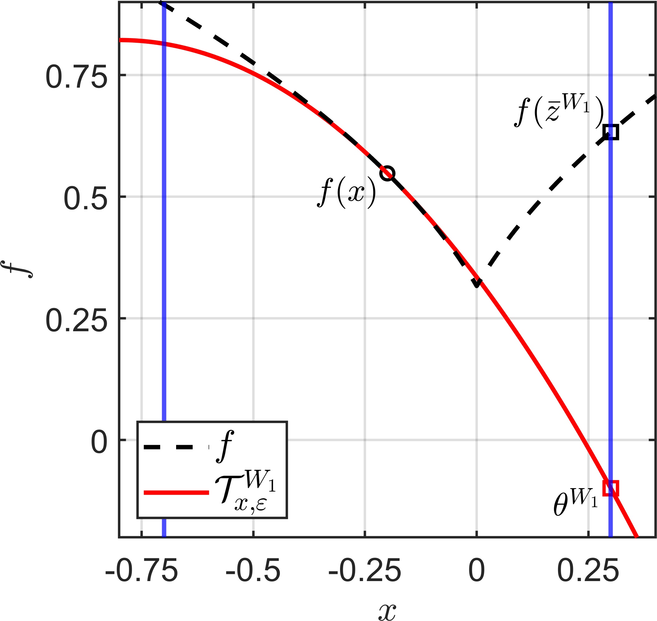
(a)

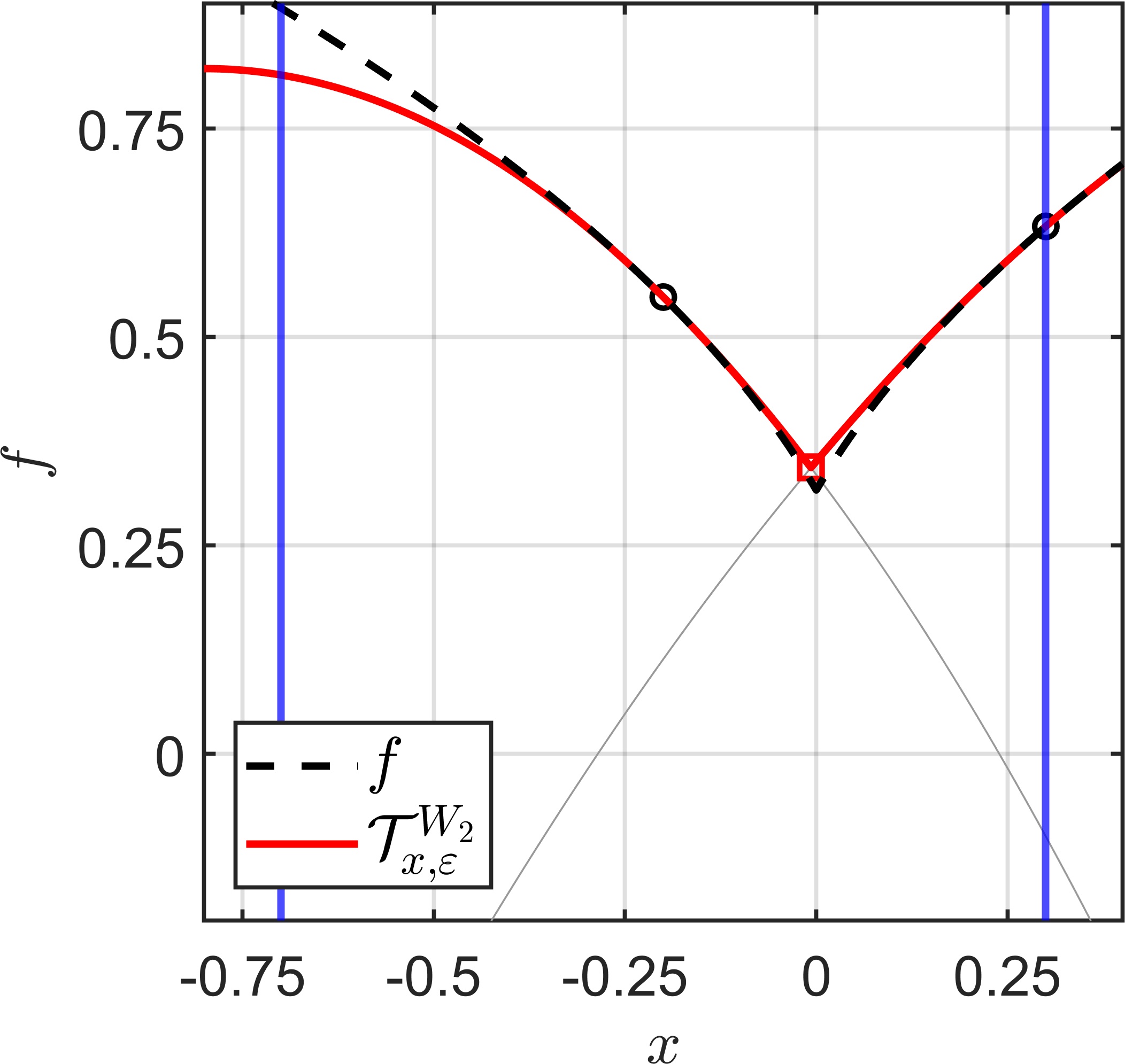
(b)

Figure 2: Visualization of our strategy for adding new elements to $W$ in Example 4.8. (The colors and markers have the same meaning as in Figure 1)

In Figure 2(a), the model $\mathcal{T}_{x,\varepsilon}^{W_{1}}$ for the initial approximation

$$W_{1}=\{(x,f(x),\nabla f(x),\nabla^{2}f(x))\}$$

is shown. While $\mathcal{T}_{x,\varepsilon}^{W_{1}}$ is a good model for $f$ locally around $x$, it clearly does not factor in the nonsmoothness of $f$, such that the minimizer $\bar{z}^{W_{1}}=0.3$ of $\mathcal{T}_{x,\varepsilon}^{W_{1}}$ does not decrease the value of $f$. Figure 2(b) shows how sampling a new element of the $\varepsilon$-jet at $\bar{z}^{W_{1}}$ and setting

$$W_{2}=W_{1}\cup\{(\bar{z}^{W_{1}},f(\bar{z}^{W_{1}}),\nabla f(\bar{z}^{W_{1}}),\nabla^{2}f(\bar{z}^{W_{1}}))\}$$

improves the approximation quality of the model. In particular, we see that the minimizer of $\mathcal{T}_{x,\varepsilon}^{W_{2}}$ is close to the actual minimizer of $f$.

The method resulting from our above considerations is shown in Algorithm 2.

Algorithm 2 Second-order $\varepsilon$-jet approximation

1:Current point $x^{i}\in\mathbb{R}^{n}$, approximation parameter $c\in(0,1)$, radius $\varepsilon>0$, improvement tolerance $\tau>0$.

2:Sample $J_{x^{i}}=(x^{i},f(x^{i}),\xi_{x^{i}},\mathcal{H}_{x^{i}})\in\mathcal{J}_{0}^{2}f(x^{i})$ and set $W=\{J_{x^{i}}\}$.

3:Compute $\theta^{W}=\theta^{W}(x^{i},\varepsilon)$ and $\bar{z}^{W}=\bar{z}^{W}(x^{i},\varepsilon)$ via (17) (or (18)).

4:If $f(\bar{z}^{W})\leq f(x^{i})+c(\theta^{W}-f(x^{i}))$ or $(\theta^{W}-f(x^{i}))/\varepsilon>-\tau$ then stop.

5:Sample $J_{\bar{z}^{W}}=(\bar{z}^{W},f(\bar{z}^{W}),\xi_{\bar{z}^{W}},\mathcal{H}_{\bar{z}^{W}})\in\mathcal{J}_{0}^{2}f(\bar{z}^{W})$, set $W=W\cup\{J_{\bar{z}^{W}}\}$ and go to step 2.

For the initialization of $W$, a single element $J_{x^{i}}\in\mathcal{J}_{0}^{2}f(x^{i})$ is sampled, but any other subset of $\mathcal{J}_{\varepsilon}^{2}f(x^{i})$ can be used as well. By Lemma 4.7, the algorithm generates a sequence $(W_{j})_{j}$ of subsets of $\mathcal{J}^{2}_{\varepsilon}f(x^{i})$ with $\theta^{W_{j+1}}\geq\theta^{W_{j}}$. Since the inequalities in step 3 are more likely to hold the larger $\theta^{W_{j}}$, the hope is that they are met at some point such that the algorithm and the sequence are finite. While an actual proof of this behavior is left for future work, the numerical experiments in Section 5 motivate us to believe that this may be the case (for a sufficiently large class of objective functions).

4.3 Practical algorithm

By using Algorithm 2 for approximating the $\varepsilon$-jet in Algorithm 1, we obtain Algorithm 3. In contrast to Algorithm 1, which required the full knowledge of the $\varepsilon$-jet, this algorithm only requires a single element of $\mathcal{J}_{0}^{2}f(x)$ for any $x\in\mathbb{R}^{n}$. (In particular, if $f$ is twice continuously differentiable on a neighborhood of $x$, then it only requires the evaluation of $f(x)$, $\nabla f(x)$ and $\nabla^{2}f(x)$.) Compared to Algorithm 2, the set $W$ in step 2 of Algorithm 3 additionally contains all elements from the previous iteration corresponding to points that also lie in $B_{\varepsilon}(x^{i})$, which (potentially) reduces the overall number of function evaluations.

Algorithm 3 Practical descent method

1:Starting point $x^{0}\in\mathbb{R}^{n}$, approximation parameter $c\in(0,1)$, initial radius $\varepsilon_{\text{init}}>0$, initial improvement tolerance $\tau_{\text{init}}>0$, reduction factors $\kappa_{\varepsilon},\kappa_{\tau}\in(0,1)$.

2:Initialize $i=0$, $\varepsilon=\varepsilon_{\text{init}}$, $\tau=\tau_{\text{init}}$ and $W=\emptyset$.

3:Sample $J_{x^{i}}=(x^{i},f(x^{i}),\xi_{x^{i}},\mathcal{H}_{x^{i}})\in\mathcal{J}_{0}^{2}f(x^{i})$ and set $W=\{J_{x^{i}}\}\cup\{J_{y}\in W:y\in B_{\varepsilon}(x^{i})\}\subseteq\mathcal{J}_{\varepsilon}^{2}f(x^{i})$.

4:Compute $\theta^{W}=\theta^{W}(x^{i},\varepsilon)$ and $\bar{z}^{W}=\bar{z}^{W}(x^{i},\varepsilon)$ via (17) (or (18)).

5:If $(\theta^{W}-f(x^{i}))/\varepsilon>-\tau$ then set $\varepsilon=\kappa_{\varepsilon}\varepsilon$, $\tau=\kappa_{\tau}\tau$ and go to step 2.

6:If $f(\bar{z}^{W})>f(x^{i})+c(\theta^{W}-f(x^{i}))$ then sample $J_{\bar{z}^{W}}=(\bar{z}^{W},f(\bar{z}^{W}),\xi_{\bar{z}^{W}},\mathcal{H}_{\bar{z}^{W}})\in\mathcal{J}_{0}^{2}f(\bar{z})$, set $W=W\cup\{J_{\bar{z}^{W}}\}$ and go to step 3.

7:Set $x^{i+1}=\bar{z}^{W}$, $\varepsilon_{i}=\varepsilon$, $\tau_{i}=\tau$, $i=i+1$ and go to step 2.

Since Algorithm 2 is applied in Algorithm 3 and we did not show that the former always terminates, the latter might get “stuck”. Nonetheless, if we assume that Algorithm 2 does always terminate (i.e., that there is no infinite loop in steps 3 to 5 in Algorithm 3), then convergence of the sequence generated by Algorithm 3 can be shown as in Theorem 4.3.

Theorem 4.9.

Assume that $f$ is convex with bounded level sets. Then Algorithm 3 generates a sequence $(x^{i})_{i}$ such that $(f(x^{i}))_{i}$ converges to the minimal value of $f$, or it enters an infinite loop in steps 3 to 5.

Proof.

Assume that there is no infinite loop in steps 3 to 5.
Case 1: $(x^{i})_{i}$ is finite. Let $x^{l}$ be the final element of $(x^{i})_{i}$. Then the condition in step 4 hast to hold infinitely many times for $i=l$, i.e., there is a sequence $(W_{j})_{j}$ of subsets $W_{j}\subseteq\mathcal{J}_{\kappa_{\varepsilon}^{j}\varepsilon_{l-1}}^{2}f(x^{l})$ such that

$$\frac{\theta^{W_{j}}-f(x^{l})}{\kappa_{\varepsilon}^{j}\varepsilon_{l-1}}>-\kappa_{\tau}^{j}\tau_{l-1}\quad\forall j\in\mathbb{N}.$$

Since $\theta^{W_{j}}\leq\theta(x^{l},\kappa_{\varepsilon}^{j}\varepsilon_{l-1})$ for all $j\in\mathbb{N}$ (cf. (19)), the proof follows as in the proof of Theorem 4.3.
Case 2: $(x^{i})_{i}$ is infinite. Note that for the algorithm to reach step 6, the conditions in step 4 and 5 must be violated. By (22), this implies

$$f(x^{i+1})\leq f(x^{i})-c\tau_{i}\varepsilon_{i}\quad\forall i\in\mathbb{N}.$$

Since $f$ is bounded below, $(\varepsilon_{i})_{i}$ and $(\tau_{i})_{i}$ must tend to zero, so the condition in step 4 has to hold infinitely many times (but not in the same iteration $i$). Thus, there is a subsequence $(x^{i_{j}})_{j}$ of $(x^{i})_{i}$ and a sequence $(W_{j})_{j}$ of subsets $W_{j}\subseteq\mathcal{J}_{\varepsilon_{i_{j}-1}}^{2}f(x^{i_{j}})$ such that

$$\frac{\theta^{W_{j}}-f(x^{i_{j}})}{\varepsilon_{i_{j}-1}}>-\tau_{i_{j}-1}\quad\forall j\in\mathbb{N}.$$

Since $\theta^{W_{j}}\leq\theta(x^{i_{j}},\varepsilon_{i_{j}-1})$ for all $j\in\mathbb{N}$, the proof follows as in the proof of Theorem 4.3. ∎

5 Numerical experiments

In this section, we will compare the performance of Algorithm 3 to the performance of the following implementations of other solution methods:

• Gradient sampling (GS) implementation from [3]

• HANSO [26]: Quasi-Newton (BFGS) method

• GRANSO [6]: Quasi-Newton (BFGS) method (for constrained problems)

• SLQPGS [7]: SQP-method combined with gradient sampling

• LMBM [18]: Limited-memory bundle method

As test problems, we choose the 20 problems from [18] (originally from [19, 28], also considered in [23]), consisting of convex and nonconvex problems. They are scalable in the number of variables $n$, and we choose $n=50$ for all problems. For the evaluation of gradients and Hessians we use the analytic formulas.

For our numerical experiments we have implemented Algorithm 3 in MATLAB (R2021a). The subproblem (18) is solved via the interior-point method (see, e.g., [34], Chapter 19) of fmincon. (If fmincon terminates in an infeasible point, we restart it using a random starting point. If it terminates in a feasible point but the optimality condition is violated, we simply use the final point as the solution.) For the parameters of Algorithm 3, we choose

$$c=0.5,\ \varepsilon_{\text{init}}=10,\ \tau_{\text{init}}=10^{-5},\ \kappa_{\varepsilon}=0.1,\ \kappa_{\tau}=1.$$

Choosing $\kappa_{\tau}=1$ means that we can not apply our theoretical convergence results, but it leads to better performance in practice in our experiments. (A similar behavior was observed for the optimality tolerance in the gradient sampling method in [3], Section 4.) We stop our method as soon as $\varepsilon<10^{-5}$ or $i>1000$. For the other five methods above, we set the maximum number of iterations to $1000$ and use the default parameters otherwise. The results are shown in Table 1.

Table 1: Result of applying Algorithm 3, GS, HANSO, GRANSO, SLQPGS and LMBM to the 20 test problems from [18] (in the same order). Listed are the number of subgradient evaluations required (#$\partial f$) and the difference to the smallest objective value found by any method (Acc.). For each problem, the values corresponding to the method with the lowest number of subgradient evaluations while having an accuracy of at least $10^{-4}$ are written in bold.

	Algo. 3		GS		HANSO		GRANSO		SLQPGS		LMBM
No.	#$\partial f$	Acc.	#$\partial f$	Acc.	#$\partial f$	Acc.	#$\partial f$	Acc.	#$\partial f$	Acc.	#$\partial f$	Acc.
1.	373	5e-14	61200	0	2125	1e-12	2125	1e-12	48581	7e-07	501	5e-06
2.	83	1e-05	20200	7e-08	988	4e-12	1447	0	12625	8e-03	1382	2e-05
3.	85	5e-06	51700	3e-06	1241	0	773	1e-08	27674	3e-06	1233	4e-03
4.	348	0	19200	6e-06	968	4e-05	1055	3e-05	31815	3e-06	750	2e-02
5.	29	2e-08	174500	3e-06	221	0	185	1e-14	4848	6e-06	62	1e-01
6.	18	4e-08	3900	1e-06	92	0	26	4e-04	29088	1e-06	97	7e-11
7.	624	1e-06	12000	2e-06	226	0	99	2e-04	15958	1e-06	2241	1e-06
8.	291	3e-05	61300	1e-05	1107	6e-06	2980	0	29492	4e-05	1894	2e-02
9.	15	1e-08	33800	2e-06	175	0	185	1e-16	5151	1e-06	307	3e-09
10.	18	4e-08	68400	2e+00	453	7e-07	878	0	79184	6e-06	4446	6e-05
11.	458	1e-07	59700	7e-09	100	0	1658	1e-08	101101	2e+01	1001	4e+01
12.	82	1e-05	10600	2e-06	573	2e-11	937	0	14342	6e-03	1529	9e-07
13.	113	0	54200	2e-07	32	3e+00	42	3e+00	14241	2e-06	48	2e+00
14.	149	4e+00	70400	4e+00	675	3e-04	1255	0	88779	4e+00	1731	6e+00
15.	883	6e-06	84600	7e-05	1254	0	486	2e-05	10807	5e-05	1821	8e-02
16.	333	3e-08	31300	0	32	2e-02	45	2e-02	9292	5e-07	1541	2e-02
17.	1226	5e-09	34600	0	2536	2e-10	2524	2e-10	11514	4e-05	7817	9e-01
18.	113	2e-10	600000	2e-01	3263	0	2615	3e-08	24644	2e-06	3087	5e-01
19.	488	0	223100	4e-04	2689	5e-04	2689	5e-04	5454	6e-04	2816	6e-04
20.	2014	0	485900	3e-02	539	4e+01	831	4e+01	52823	3e-03	128	4e+01

For each method and each test problem, it contains the number of subgradient evaluations and the distance of the final objective value to the smallest objective value found by any method for the respective problem. For Algorithm 3, the number of subgradient evaluations coincides with the number of Hessian evaluations and is by one smaller than the number of $f$ evaluations. For HANSO, GRANSO and LMBM, the subgradient evaluations coincide with the $f$ evaluations and for GS and SLQPGS, the number of $f$ evaluations is significantly smaller than the number of subgradient evaluations.

If we consider a method to be convergent on a problem if the difference between its final objective value and the best objective value found by any method is less than $10^{-4}$, then Algorithm 3 has the lowest number of subgradient evaluations of all convergent methods for $16$ of the $20$ test problems. For problem $14$, Algorithm 3 finds a point which is only locally optimal and for problems $7$, $11$ and $15$, it requires more subgradient evaluations than other methods. (Note that this is not a perfect way to compare the methods, since one method may require more subgradient evaluations than another method while computing better solutions. In theory one should try to choose the parameters of the methods such that they all produce solutions of the same quality, but this is difficult due to the diversity of their stopping criteria.)

We can further analyze the results in Table 1 by considering so-called performance profiles [10]. Figure 3 shows the performance profile resulting from Table 1 when using the number of subgradient evaluations as the performance measure.

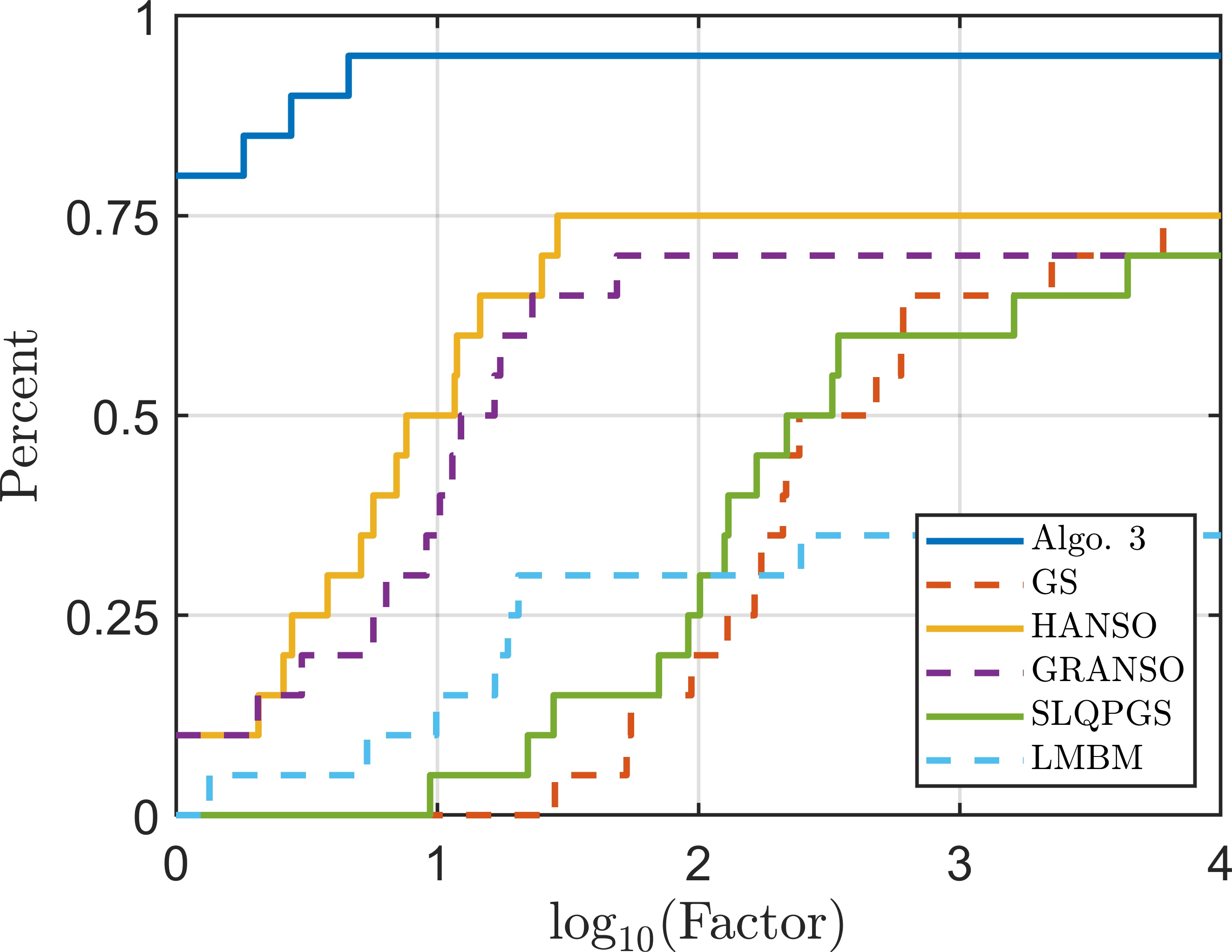
Figure 3: Performance profile resulting from Table 1 when using the number of subgradient evaluations as performance measure (and the accuracy $10^{-4}$ as convergence threshold)

For each method, it shows what percentage of the $20$ test problems can be solved (meaning that the accuracy is less than $10^{-4}$) while not performing worse than a certain factor of the best performing method on each problem. More formally, the curve of a method passing through a point $(r,p)$ in Figure 3 means that $p$ percent of the 20 test problems can be solved by the method while not using more than $10^{r}$ times the number of subgradient evaluations of the best performing method on each problem. We see that Algorithm 3 is either the best performing method or within a (relatively) small factor of the best performing method for all test problems (except problem $14$).

While the results above suggest that Algorithm 3 is more efficient than the other methods in terms of function evaluations, we have to emphasize that it requires Hessian matrices, which may be costly to evaluate in practical applications. Furthermore, the MATLAB implementation we used here is worse in terms of the actual runtime. For example, for test problem $4$, our implementation took $71$ seconds while HANSO only took $0.2$ seconds despite having more than twice the number of subgradient evaluations. The reason for the worse runtime is the fact that function evaluations take almost no time in our examples and the subproblem (18) has to be solved many times in our algorithm. In contrast to the subproblems of other methods, (18) can not be solved as a (convex) quadratic problem. Thus, for the numerical experiments for this article, we simply treated it as a general nonlinear optimization problem, which makes its solution relatively time-consuming. To improve the runtime of our method (for examples where the evaluation of the objective function and its derivatives is cheap), future work in this area should include the construction of a dedicated and efficient solver for this subproblem that exploits its structure.

6 Conclusion and outlook

In this article, we have constructed a descent method for nonsmooth optimization problems based on a model of the objective function involving second-order derivative information. We started by defining and analyzing our concept of second-order information, the second-order $\varepsilon$-jet, which is essentially the set of all coefficients of second-order Taylor expansions of the objective in an $\varepsilon$-ball. Taking the maximum over all these Taylor expansions yields a model of the objective. We then showed that iterative minimization of this model (constrained to the $\varepsilon$-ball) can be used for the minimization of the original function, and we proved convergence of the resulting algorithm to minimal points for the convex case. Since this first algorithm unrealistically assumed full knowledge of the $\varepsilon$-jet, we then constructed an approximation scheme for the $\varepsilon$-jet (based on sampling finitely many elements) that can be incorporated into the algorithm to obtain an implementable method (Algorithm 3). We showed convergence of Algorithm 3 in case the approximation scheme always terminates. Using a set of test problems, we compared the performance of Algorithm 3 to the performance of five other available solvers. While the results can not directly be compared due to the reliance of our method on the availability of Hessian matrices, they suggest that the proposed method is more efficient in terms of function evaluations than standard gradient sampling, and (at least) competitive compared to other methods.

There are several open questions in this work for future research:

• As mentioned in the numerical experiments, the subproblem (18) resulting from minimizing our model is more difficult to solve than the subproblems of other methods, since it can not be solved as a convex quadratic problem. While it can be treated as a general nonlinear problem, it clearly possesses structure that can potentially be exploited in a specialized solver. Alternatively, it could be worth it to analyze the behavior of Algorithms 1 and 3 when only approximated solutions of the subproblem are used.

• Although we only proved convergence of the (theoretical) Algorithm 1 for the convex case, our numerical experiments suggest that it also works for (a reasonably large class of) nonconvex functions, giving us hope that convergence can be proven in the nonconvex case as well. A theoretical approach that could be useful for this is the consideration of the first-order optimality conditions of the subproblem (9), for which the subdifferential of the model $\mathcal{T}_{x,\varepsilon}$ may be derived as in [17].

• For Algorithm 2, we only showed that it generates a sequence of approximations of the $\varepsilon$-jet with a new (previously unknown) element in every iteration, but we did not prove that it actually terminates.

• A theoretical analysis of the convergence rate of Algorithm 1 (and Algorithm 3) should be carried out to verify the observation of improved performance in the numerical experiments.

Additionally, there are possible modifications to our approach that could lead to other interesting variants of our method:

• Clearly, the reliance of our method on the availability of Hessian matrices is a strong assumption which rules out many applications. It seems natural to think about Quasi-Newton strategies to avoid exact Hessians, but the generalization of these strategies to our nonsmooth case is not trivial. First of all, in our setting, the “Hessian” $\operatorname*{pr}_{4}(\mathcal{J}_{\varepsilon}^{2}f(x))$ is actually a set of matrices instead of a single matrix, so the common update formulas can not directly be used. Furthermore, our method uses $4$-tuples $(y,f(y),\xi,\mathcal{H})\in\mathcal{J}_{\varepsilon}^{2}f(x)$, so every matrix $\mathcal{H}$ has an associated point $y$ and subgradient $\xi$. Nonetheless, it is worth noting that in our convergence theory, the actual properties of $\mathcal{H}$ of being a Hessian matrix (or a limit of a sequence of Hessian matrices) of $f$ was never used, so we expect our method to be relatively robust when using approximated Hessians instead of exact Hessians.

• The idea of constraining $\mathcal{T}_{x,\varepsilon}$ to the $\varepsilon$-ball is similar to the well-known idea of trust-region methods. But in contrast to classic trust-region methods, our approach does not contain a mechanism for increasing the radius $\varepsilon$. While such a mechanism appears to be unnecessary for the problems we considered in our numerical experiments, we expect that it could greatly improve the performance for other types of objective functions.

References

- [1] A. Bagirov, N. Karmitsa, and M. M. Mäkelä. Introduction to Nonsmooth Optimization. Springer International Publishing, 2014.
- [2] J. V. Burke, F. E. Curtis, A. S. Lewis, M. L. Overton, and L. E. A. Simões. Gradient Sampling Methods for Nonsmooth Optimization. In Numerical Nonsmooth Optimization, pages 201–225. Springer International Publishing, 2020.
- [3] J. V. Burke, A. S. Lewis, and M. L. Overton. A Robust Gradient Sampling Algorithm for Nonsmooth, Nonconvex Optimization. SIAM Journal on Optimization, 15(3):751–779, Jan. 2005.
- [4] F. H. Clarke. Optimization and Nonsmooth Analysis. Society for Industrial and Applied Mathematics, Jan. 1990.
- [5] R. Cominetti and R. Correa. A Generalized Second-Order Derivative in Nonsmooth Optimization. SIAM Journal on Control and Optimization, 28(4):789–809, May 1990.
- [6] F. E. Curtis, T. Mitchell, and M. L. Overton. A BFGS-SQP method for nonsmooth, nonconvex, constrained optimization and its evaluation using relative minimization profiles. Optimization Methods and Software, 32(1):148–181, 2017.
- [7] F. E. Curtis and M. L. Overton. A Sequential Quadratic Programming Algorithm for Nonconvex, Nonsmooth Constrained Optimization. SIAM Journal on Optimization, 22(2):474–500, Jan. 2012.
- [8] F. E. Curtis and X. Que. A quasi-newton algorithm for nonconvex, nonsmooth optimization with global convergence guarantees. Mathematical Programming Computation, 7(4):399–428, May 2015.
- [9] L. Danzer, B. Grünbaum, and V. Klee. Helly’s Theorem and Its Relatives. Proceedings of Symposia in Pure Mathematics: Convexity, 1963.
- [10] E. D. Dolan and J. J. Moré. Benchmarking optimization software with performance profiles. Mathematical Programming, 91(2):201–213, Jan. 2002.
- [11] L. C. Evans and R. F. Gariepy. Measure Theory and Fine Properties of Functions, Revised Edition. Chapman and Hall/CRC, Apr. 2015.
- [12] B. Gebken and S. Peitz. An Efficient Descent Method for Locally Lipschitz Multiobjective Optimization Problems. Journal of Optimization Theory and Applications, 80:3–29, Mar. 2021.
- [13] A. A. Goldstein. Optimization of lipschitz continuous functions. Mathematical Programming, 13(1):14–22, Dec. 1977.
- [14] M. Golubitsky and V. Guillemin. Stable Mappings and Their Singularities. Springer US, 1973.
- [15] I. Goodfellow, Y. Bengio, and A. Courville. Deep Learning. MIT Press, 2016. http://www.deeplearningbook.org.
- [16] A. Grothey. A Second Order Trust Region Bundle Method for Nonconvex Nonsmooth Optimization. Technical report MS-02-005, University of Edinburgh, Edinburgh, 2002.
- [17] N. X. Ha and D. Van Luu. Invexity of supremum and infimum functions. Bull. Aust. Math. Soc., 65(2):289–306, 2002.
- [18] M. Haarala. Large-scale nonsmooth optimization: variable metric bundle method with limited memory. PhD thesis, University of Jyväskylä, 2004.
- [19] M. Haarala, K. Miettinen, and M. M. Mäkelä. New limited memory bundle method for large-scale nonsmooth optimization. Optimization Methods and Software, 19(6):673–692, Dec. 2004.
- [20] E. S. Helou, S. A. Santos, and L. E. A. Simões. On the local convergence analysis of the gradient sampling method for finite max-functions. J. Optim. Theory Appl., 175(1):137–157, Oct. 2017.
- [21] C. Horvath. Measure of non-compactness and multivalued mappings in complete metric topological vector spaces. Journal of Mathematical Analysis and Applications, 108(2):403–408, June 1985.
- [22] A. Ioffe and J.-P. Penot. Limiting subhessians, limiting subjets and their calculus. Transactions of the American Mathematical Society, 349(2):789–807, 1997.
- [23] N. Karmitsa, A. Bagirov, and M. M. Mäkelä. Comparing different nonsmooth minimization methods and software. Optimization Methods and Software, 27(1):131–153, 2012.
- [24] K. C. Kiwiel. Methods of Descent for Nondifferentiable Optimization. Springer Berlin Heidelberg, 1985.
- [25] K. C. Kiwiel. Convergence of the Gradient Sampling Algorithm for Nonsmooth Nonconvex Optimization. SIAM Journal on Optimization, 18(2):379–388, Jan. 2007.
- [26] A. S. Lewis and M. L. Overton. Nonsmooth optimization via quasi-Newton methods. Mathematical Programming, 141:135–163, 2013.
- [27] L. Lukšan and J. Vlček. A bundle-newton method for nonsmooth unconstrained minimization. Mathematical Programming, 83(1-3):373–391, Jan. 1998.
- [28] L. Lukšan, M. Tůma, and K. Šiška. UFO 2002. Interactive System for Universal Functional Optimization. Technical Report 883, Institute of Computer Science, Academy of Sciences of the Czech Republic, Prague, 2002.
- [29] N. Mahdavi-Amiri and R. Yousefpour. An Effective Nonsmooth Optimization Algorithm for Locally Lipschitz Functions. Journal of Optimization Theory and Applications, 155(1):180–195, Apr. 2012.
- [30] R. Mifflin. Better than linear convergence and safeguarding in nonsmooth minimization. In System Modelling and Optimization, pages 321–330. Springer-Verlag, 1984.
- [31] R. Mifflin and C. Sagastizábal. A science fiction story in nonsmooth optimization originating at IIASA. Documenta Mathematica, 2012.
- [32] E. S. Mistakidis and G. E. Stavroulakis. Nonconvex optimization in mechanics. Nonconvex optimization and its applications. Springer, New York, NY, Nov. 1998.
- [33] B. S. Mordukhovich and J. V. Outrata. On Second-Order Subdifferentials and Their Applications. SIAM Journal on Optimization, 12(1):139–169, Jan. 2001.
- [34] J. Nocedal and S. Wright. Numerical Optimization. Springer New York, 2006.
- [35] S. Scheimberg and P. R. Oliveira. Descent algorithm for a class of convex nondifferentiable functions. Journal of Optimization Theory and Applications, 72(2):269–297, Feb. 1992.
- [36] A. Seeger. Limiting behavior of the approximate second-order subdifferential of a convex function. Journal of Optimization Theory and Applications, 74(3):527–544, Sept. 1992.
- [37] R. Tibshirani. Regression Shrinkage and Selection via the Lasso. Journal of the Royal Statistical Society: Series B (Methodological), 58(1):267–288, Jan. 1996.
- [38] M. Ulbrich. Semismooth Newton Methods for Operator Equations in Function Spaces. SIAM Journal on Optimization, 13(3):805–841, Jan. 2002.
- [39] J. Zowe. Nondifferentiable Optimization. In Computational Mathematical Programming, pages 323–356. Springer Berlin Heidelberg, 1985.