Topological invariants based on generalized position operators and application to the interacting Rice-Mele model
Abstract
We discuss different properties and the potential of several topological invariants based on position operators to identify phase transitions, and compare with more accurate methods, like crossing of excited energy levels and jumps in Berry phases. The invariants have the form , where is the length of the system, the position of the site , and the operator of the number of particles at site with spin . We show that should be integers, and in some cases of magnitude larger than 1 to lead to well defined expectation values. For the interacting Rice-Mele model (which contains the interacting Su-Schrieffer-Heeger and the ionic Hubbard model as specific cases), we show that three different invariants give complementary information and are necessary and sufficient to construct the phase diagrams in the regions where the invariants are protected by inversion symmetry. We also discuss the consequences for pumping of charge and spin, and the effect of an Ising spin-spin interaction or a staggered magnetic field.
I Introduction
Many transitions in condensed matter has been understood as a spontaneous symmetry breaking and the emergence of a local order parameter as the temperature is lowered landau . However, there are other transitions, which are the subject of much attention recently, in which two different phases differ in the value of a symmetry protected topological invariant cla ; kita ; hasan ; slag ; ando ; chiu ; brad ; krut ; wang ; ari . While significant advances have been made at the single-particle level, more recent studies have addressed many-body cases chiu ; ari ; gur ; man ; unan ; ari2 ; osta .
A difference with the non-interacting case is that the presence of zero-energy edge modes dictated by the bulk-boundary correspondence, is modified by the possible presence of zeros of the interacting Green’s functions at zero energy gur ; man . Interestingly, these zeros are responsible for a topological transition in a two-channel spin-1 Kondo model with easy-plane anisotropy fepc .
Many of the topological invariants used are extensions of the Berry phase calculated by Zak for a one-particle state as the wave vector sweeps the entire Brillouin zone in one dimension zak (see for example Refs. ando, ; osta, ; tewa, ; asb, ; carda, ; diag, ). This charge Berry phase is in turn the basis of the modern theory of polarization pola1 ; pola2 ; pola3 ; bradlyn , and has been extended to the many-body case om ; resor ; oc ; song and to multipoles whee ; tahir . Changes in are proportional to changes in the polarization of the system om . We have introduced the spin Berry phase , which is a measure of the difference of polarizations between electrons with spin up and down gs .
In systems with inversion symmetry, both phases are protected by this symmetry and can take only the values 0 or . Thus, they are topological invariants and have been used to identify quantum phase transitions om ; phtopo ; dipol ; phihm ; tprime and in particular to construct the phase diagram of the Hubbard chain with correlated (density-dependent) hopping (HCCH) phtopo and the ionic Hubbard chain (the Hubbard model with alternating on-site energies discussed in more detail in Section IV) phihm . Furthermore for these two models, it has been shown phihm that the jumps of the Berry phases coincide with crossings of energy levels which are known to correspond to phase transitions determined by the method of crossing of excited energy levels (MCEL) based on conformal field theory nomu ; naka ; naka1 ; naka2 ; som . Therefore, the results extrapolated to the thermodynamic limit are expected to be highly accurate and more efficient than calculating correlation functions, which change in a smooth fashion at the transitions in finite systems. For the HCCH the phase diagram obtained from jumps in the Berry phases coincides with that obtained from bosonization jaka ; bosolili for small values of the interaction.
Using results of the MCEL naka , it has been shown that for systems with spin SU(2) symmetry, the jump of the spin Berry phase indicates the opening of a spin gap gs . In a Kosterliz-Thouless transition, the spin gap opens exponentially at it is very difficult to identify the transition point from a direct calculation of the spin gap in large systems. It is much more efficient to determine these point extrapolating the jumps in the topological invariant for small systems phtopo
Resta zresta ; resorz has shown (for an integer number of particles per unit cell) that in the thermodynamic limit, the polarization and the charge Berry phase, can be calculated from a ground state expectation value as with
| (1) |
where
| (2) |
is the length of the system, the position of the site , the operator of the number of particles at site , and are integers. Although this expectation value is expected to be less accurate than the charge Berry phase for a finite system, it is easier to calculate, and has been used extensively. For a non-interacting system, Resta has shown that coincides with the charge Berry phase in the thermodynamic limit zresta . One expects that this is also true in the interacting case. This is supported by our calculations in a specific interacting model presented in Section VI.1.
Soon it was noticed that in turn, at zero temperature, is an approximation to the spin Berry phase phtopo , which is expected to coincide with it (except for a sign, as explained in Section III) in the thermodynamic limit.
If the total number of particles per unit cell is an irreducible fraction , is ill defined and should be replaced by zl . In general, the conditions that should fulfill to lead to well defined are discussed in Section III. The quantity
| (3) |
where is the lattice parameter, is a well defined expectation value of the sum of the positions of the particles per unit cell zl ; zl2 . Recently it has been shown that is a topological invariant at finite temperature unan . At zero temperature, the quantity pointed out in Ref. phtopo, as an alternative to calculate the spin the Berry phase for , was used by Nakamura and Todo to study resonance-valence-bond states in spin systems todo , using the symmetry properties explained in Ref. zl, . The operator of Eq. (2) has also being generalized as a tensor for different spin and position directions, allowing to express the ferrotoroidic moment as a quantum geometric phase ferrot . Cumulants of cum0 ; cum1 were also used to identify phase transitions cum ; het1 ; het2 , and was used to study scaling in disordered systems het3 .
A Thouless pump can be regarded as a cycle in a space of parameters in which a quantized amount of charge (or spin) is transported, which is topologically protected thou ; niu . Experimentally quantized charge pumping has been realized in ultracold quantum-gas experiments that simulate the fermionic nakaji and bosonic loh Rice-Mele model (RMM) rice . A spin pump was also realized experimentally schw2 . Recently charge pumping in the fermionic interacting RMM (IRMM) has been studied experimentally konrad and theoretically nakag ; stenz ; eric . For a recent review of Thouless pumping and topology, see Ref. citro, .
The RMM contains the Su-Schrieffer-Heeger model (SSHM) su as a special case, with alternating hopping matrix elements . For the spinless SSHM or the non-interacting case choosing one spin, two different topological states exists depending on the sign of , which are characterized by different Zak Berry phases, either 0 or mod asb . While the charge and spin transport in the adiabatic limit of the IRMM can be well described in terms of the charge and spin Berry phases described above, or equivalently by and eric , these quantities are unable to separate the two topological phases of the SSHM. This is expected, because since the average position (or polarization) of the particles for both spins is the same, and 0 or mod , adding or subtracting them gives 0 mod in both cases. Recently, a study of the SSHM at finite temperatures found in some cases moli . In addition, in a recent study on the strongly-interacting SU(3) SSHM, it has been stated that a Berry phase in which the flux is applied only to one of the flavors [related to or in the SU(2) case] can distinguish between the two topological sectors.
In this paper we discuss for the general case, the conditions on the so that the generalized position operators are well defined. They should be integers and it is convenient to choose them as the smallest possible integers that guarantee translationally invariant position operators. We also study their properties under inversion and their relation with the Berry phases. The discussion is restricted to one dimension and two flavors, but it can be generalized. For the specific IRMM, and parameters for which the system has inversion symmetry, we compare the topological transitions predicted from jumps in several with alternative methods. The size dependence of the transitions is also studied. We find that to obtain a complete picture of the topological sectors, three different invariants should be considered, , and either or . We also discuss the effect of terms that open the spin gap, like an Ising interaction and staggered magnetic field eric . Finally we used the generalized position operators to analyze the charge and spin transport in pump cycles.
The paper is organized as follows. In Section II we briefly review the calculation of the Berry phases and its relation to the modern theory of polarization in the many-body case. This facilitates the explanation of the position expectation values and its symmetry properties for general Hamiltonians discussed in Section III. In Section IV we explain the IRMM with possible addition of Ising spin-spin interactions and staggered magnetic field, which is used for numerical calculations in Section VI. In Section V we discuss the form of some general symmetry properties discussed in Section III to particular cases of the IRMM. In Section VI we present different calculations using exact diagonalization, in systems up to 14 sites, to compare the predictions of the phase transitions obtained from jumps in the topological invariants based on position operators, with other (in general more robust) known results. We also study some pump cycles which shed light on the potential and limitations of the different position operators. Section VII contains a summary and discussion.
II Berry phases and many-body polarization
For the discussion of the topological invariants, it is useful to briefly review the formulation of the Berry phases and the modern theory of polarization for many-body systems. This theory is basically an extension of the formalism of Zak for non-interacting particles zak . Restricting to one-dimension, Zak calculated the Berry phase of a Bloch state as the wave vector sweeps all possible values , where is the lattice parameter. This is equivalent to consider all possible twisted boundary conditions defined by a flux through a ring. To simplify the argument, ignore spin for the moment and consider that the hopping term of the Hamiltonian has the form (extension to more involved cases are straightforward)
| (4) |
where is the number of sites. The Hamiltonian can be interpreted as a periodic chain with boundary conditions such that a translation of a one-particle state in the size of the system , where is the number of unit cells, gives
| (5) |
The eigenstates of the translation operator with a given wave vector satisfy
| (7) |
with integer. Then, changing adiabatically the flux is equivalent to changing the one-particle wave vectors.
For a periodic many-body system with conserved number of particles , the total wave vector is conserved, and the change in under an adiabatic change in is given by
| (8) |
Then, if the number of particles per unit cell is an integer, and if a given state (in particular the ground state) is non degenerate as is swept from to , the ground state returns to the ground state and captures a Berry phase. If however, is fractional, the state at is different from that at (it has a different total wave vector) and the cycle should be extended to the region , with integer gs ; zl
In practice, it is convenient to perform a gauge transformation
| (9) |
where is the position of the site , so that the hopping term becomes explicitly translationally invariant
| (10) | |||||
where is the nearest-neighbor distance. In the more general cases studied below, we take also a translationally invariant form of the Hamiltonian.
The Berry phases considered here can be calculated from the numerically gauge invariant formulation om ; gs , splitting the interval of the flux in parts.
| (11) | |||||
where is the ground state of the Hamiltonian in which the hopping from site to site for spin has been changed by a factor and , given by Eq. (2) transforms the ground state for to that for using the gauge transformation Eq. (9). Usually the origin of coordinates is chosen at an atomic position. If not, the Berry phase is modified by a constant as explained in Section III. In practice, a number of splittings is enough to obtain accurate results.
The cases related with total charge om ; gs and total spin gs have been studied before. From the modern theory of polarization in the many-body case, one knows that if the parameters of the Hamiltonian are changed as a function of a parameter , between and the change of polarization (equivalent to the displacement of charge in one dimension), can be expressed in terms in the Berry phase . If the particles are electrons, the transported charge in units of where is the electronic charge, the transported charge is given by
| (12) |
Similarly for the transported projection of the spin one has gs
| (13) |
One is tempting to suggest that similar expressions could be used for in terms of and respectively. This is true in some cases, but not always. We return to this point later for the specific case of the IRMM.
In systems with inversion symmetry, and choosig the origin of coordinates at the inversion point, the result for the Berry phases should be the same if the sign of the flux is inverted, which in turn leads to same Berry phase with the sign inverted implying mod zak . Thus, in systems with inversion symmetry, is a topological number protected by symmetry that can take only two values, or mod . This fact has been used to construct the complete phase diagram of the Hubbard model with density-dependent hopping phtopo and the ionic Hubbard model phihm from the values of and or crossing of excited energy levels nomu ; naka ; naka1 ; naka2 which coincide with jumps in these Berry phases for these models phihm . In presence of a rotation symmetry of the spin in around any axis perpendicular to the axis [in particular in the presence of spin SU(2) symmetry], is also a topological number protected by that symmetry eric .
III Generalized position expectation values
Generalizing previous developments, one can define position expectation values from Eqs. (1) and (2). In addition to the total position Eq. (3) , one can define the expectation value of the sum of the positions of the electrons with spin up per unit cell as
| (14) |
where is the lattice parameter, and similarly for spin down. For , the difference between the positions of the electrons with spin up and down per unit cell is
| (15) |
In this Section we discuss the general properties of this quantities as well as some conditions imposed by symmetry.
Comparing Eqs. (1), (2) and (11) one realizes that except for the sign, the second member of Eq. (1) is a crude approximation to , with only point in the whole interval of flux . However, both quantities are expected to coincide in the thermodynamic limit zresta , has the advantage over the Berry phases of its simplicity, its extension to finite temperature and the possibility to calculate if for open boundary conditions li , which allows for more accurate density-matrix renormalization-group calculations. In addition, we find that in certain cases it is difficult to calculate directly because of level crossings that take place at finite values of the flux .
In a ring, the positions of the particles are defined modulo . This means that that should be satisfied. Thus for to be well defined, the result should be invariant if for any , is replaced by . Since the eigenvalues of are either 0 or 1, the change in the exponent of Eq. (2) is a multiple of (irrelevant) for any states if and only if the are integers.
Under an elemental translation in a unit cell one has
| (16) | |||||
where is the operator of the total number of particles with spin . For the last equality we used that any two commute.
To be well defined, should not depend of the unit cell in which the origin of is chosen. Thus, the exponential should be equivalent to 1, and this imposes
| (17) |
The first member should be a conserved quantity of the Hamiltonian. Eq. (17) implies in particular that for to be well defined, the total number of particles should be conserved, and if the number of particles per unit cell is an irreducible fraction, should be chosen as the denominator (as shown before with a slightly different argument zl ). For , the total spin projection should be conserved. In the simplest case , it is convenient to choose . Finally if and , it is convenient to choose the minimum that satisfies that is an integer. In usual cases with , and one particle per unit cell or less, this is two times larger than the corresponding one for .
The above mentioned conservation laws imply that for an extension to finite temperatures of unan , the canonical ensemble should be used. This fact seems to have been overseen in a recent work moli .
Note that Eq. (16) is also valid if the lattice parameter is replaced by any finite displacement . Following the same procedure as above, it is easy to see that
| (18) |
where is the integer entering Eq. (17). While the symmetry properties defined below take a different form for different , this constant shift is however not important, since only differences in polarization have a physical meaning [see Eqs. (12) and (13)] and the magnitude of the jumps of at phase transitions remain the same.
While the calculation of the Berry phases imply an average over all twisted boundary conditions (BC), the calculation of the displacement operators are usually performed either for closed shell BC (CSBC), which correspond to antiperiodic BC for multiple of four and periodic BC for even not multiple of four, or for open shell BC (OSBC) in which periodic and antiperiodic BC are interchanged with respect to CSBC. The results for both cases are compared in Sections VI.1 and VI.2.
If the Hamiltonian is invariant under inversion through certain atoms and the coordinates are defined in such a way that for one of these atoms , then using translations [Eq. (16)], one can define such that . Clearly
| (19) |
where the bar over means complex conjugation. Since all eigenstates should be either even or odd under , the expectation value of should be real and this implies that the second member of Eq. (1) is either or , implying that it is a topological invariant protected by .
If however the inversion symmetry has the invariant point at between two atoms, one can define , which is equivalent to a change of sign of plus a translation giving
| (20) | |||||
Implications for the particular case of the IRMM are discussed in Section V.
Note that the arguments above about topological protection by inversion symmetry applied to zero temperature, assume a non-degenerate ground state and breaks down in the thermodynamic limit if there is a spontaneous symmetry breaking. We return to this point in Section VI.3.
IV Model
To test explicitly the properties of different generalized position operators and its accuracy as topological invariants to determine phase transitions, we consider the interacting Rice-Mele model (IRMM). The Hamiltonian is
| (21) | |||||
For some calculations, we will also add to the Hamiltonian either an Ising spin-spin coupling or a staggered magnetic field eric
| (22) |
For , the model reduces to the ionic Hubbard model (IHM) phihm ; sdi ; manih , which has inversion symmetry with center at any site, and for , it coincides with the interacting SSHM (ISSHM) which has inversion symmetry with center at the midpoint between any two sites. In both cases, the Berry phases and the position operators become topological invariants protected by the corresponding inversion symmetry. Our discussion here is limited to zero temperature, number of particles equal to the number of sites () and total spin . Then, there are two particles per unit cell () and the smallest integers are enough to have well defined Berry phases and position operators [see Eqs. (3) and (14)] (this is not the case for extensions of the model to more sites per unit cell abn ).
Therefore, in the following we define , , , and , for the charge, spin and spin only expectation values. We take the position of lattice site 0 as the origin () [if the origin were taken between two lattice sites, so that , would be shifted by , by and would remain the same according to Eq. (18)].
The phase diagram of the IHM has been determined accurately using topological invariants phihm . A numerical study of different correlation functions has been performed by Manmana et al. manih . The half-filled IHM hosts three phases. For , there are only two phases, a band insulating (BI) phase with alternating occupancies 0202… or 2020… depending on the sign of for and a Mott insulating phase with one-particle per site, described by an effective Heisenberg model rihm for . At finite , a spontaneously dimerized insulator (SDI) with a bond-ordering wave (BOW) sdi appears between the other two phases and the boundaries move to larger phihm . At the BI to SDI transition, the charge Berry phase jumps from 0 to , while at the SDI to MI transition, the spin Berry phase jumps from 0 to .
The BOW corresponds to stronger expectation values of the hopping for odd than even bonds or conversely [see Eq. (27)]. The SDI corresponds to one of these choices in the thermodynamic limit. A finite breaks the inversion symmetry and renders one of the BOW phases more favorable than the other, and also the MI phase is converted to a BOW phase eric .
V Properties of the position operator with a given spin in the IRMM
According to the constraints imposed by symmetry presented in Section III, it is convenient to choose in Eq. (14) and its equivalent for spin down. The ISSHM (case of the IRMM) has inversion centers at the midpoint between two atomic positions, displaced a quarter of a unit cell from the atomic positions. Choosing the origin of coordinates at an atomic position, this implies that the inversion centers are located at plus a multiple of . Using the filling conditions assumed , and , Eq. (20) leads to
| (23) |
and the same for spin down. This implies that the expectation values of and are purely imaginary in the ISSHM. Therefore from Eq. (1) ( and ) can only take the values mod . Performing a similar calculation for and it is easy to see that and can only take the values 0 or mod .
As an example, for , and , the ground state is . Using , where , a straightforward calculation gives , and then mod Changing the sign of corresponds to a translation of half a lattice parameter and the change sign.
A simple argument, validated by the numerical results presented below, is that for any parameters of the ISSHM, the expectation values of the position operators for a given spin are the same as the corresponding ones in which one has one localized particle at the midpoint of each strong bond. For negative , this means that the position of the particles with given spin are at , to . Then , and using Eq. (1)
| (24) |
where the last line was obtained from a translation of half a lattice parameter. Eqs. (24) are confirmed by the numerical calculations.
While for , the system described by has inversion symmetry at each lattice site [implying Eq. (19)] and for , the inversion points lie in between sites [implying Eq. (23)], at the special point both symmetry operations are present, and these equations imply that the expectation values of and should vanish. This fact suggests that the phases jump at this point. Numerically we find that jumps between and for fixed changing and between and for fixed changing . The first jump is consistent with the two different topological sectors of the ISSHM man and spin models related with it tzeng as discussed in Section VI.2.
For , and very small , the second jump is expected from the phases for the states with occupancies 2020… and 0202… at both sides of the transition. Symmetry protection allows to extend the argument to large . However, the physical meaning it of the jump in the interacting case (for which the system is in the MI phase of the IHM) is not clear.
VI Numerical results
In this Section we present results for the ground-state expectation value of the different position operators by exact diagonalization in systems between 6 and 14 sites, using the Lanczos method lanc . We analyze the transitions of the corresponding topological invariants in the IHM and ISSHM and its size dependence and compare them with alternative methods. This information is complemented studying pumping cycles in the general IRMM, including a staggered field and Ising spin-spin interactions.
VI.1 Topological invariants in the IHM
As briefly explained in Section I, the phase diagram of the IHM has been determined by the MCEL which coincides with a jump in () for the charge (spin) transition between BI and SDI (SDI and MI) phases (see Section IV for the explanation of the phases). Specifically the charge transition is determined by a crossing between the singlet state of lowest energy with even parity under inversion (the ground state in the BI phase) and the corresponding one for odd parity (the ground state in the SDI and MI phases) with OSBC [see Section II for a discussion on the boundary conditions (BC)]. In the spin transition between SDI and MI phases, for OSBC the excited even singlet crosses with the excited odd triplet, which has less energy in the MI phase phihm ; eric .
To what extend do the topological invariants based on position operators reproduce these results?
The different are protected by inversion symmetry with center at each site and can take the values 0 or mod (see Section III). We find that [see Eq. (14)] do not change at the transitions and has the value 0 () if the number of unit cells is even (odd). We discuss this result in Section VI.3. Instead, extrapolating the results of the jumps in and for adequate BC provide rather precise results.
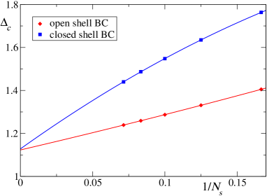
In Fig. 1 we display the results for the jump in at the charge transition for different system sizes and BC. We find that for most system sizes and OSBC, the value of at the jump coincides with the above mentioned crossing of levels. For 14 sites, predicts a larger (by about 0.003), but the difference is smaller than the size of the symbols in the figure. The results for CSBC have a larger size dependence, but the extrapolation to the thermodynamic limit using a parabola in for both sets of BC are very near each other ( for OSBC, for CSBC). The parabola seems to fit well the data. In contrast, is expected to have a power-law dependence with a model-dependent exponent koba .
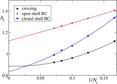
In Fig. 2 we show the results of the spin transition and the more reliable result using the MCEL. A problem with the OSBC is that for both and change abruptly with the ground state crossing with change of parity, and both and coincide. For 14 sites is smaller as expected, but the difference is very small. Larger system sizes would be needed to correct this result. For the spin transition, the CSBC are more reliable, predicting an extrapolated value compared to of the MCEL.
VI.2 Topological transitions in the ISSHM including
Here we consider the Hamiltonian , where the two terms are given in Eqs. (21) and (22), with . The motivation is that for large , this Hamiltonian reduces to an XXZ Heisenberg model with alternating bond interactions eric similar to that studied by Tzeng et al. tzeng . This model has three phases, a Néel phase for small and two topologically different dimerized phases for large negative or positive .
From the results of Section V one knows that the different are topological invariants protected by inversion symmetry with center at the midpoint between any two sites. In Fig. 3 we show the different invariants as a function of . For , the system is in the MI phase of the IHM. As no charge transition takes place, retains the same value for finite . Instead, shows jumps consistent with a transition from a Néel state at small to dimerized BOW phases at large . In contrast, does not capture this transition, but it is able to differentiate between both BOW phases.
These results can be understood in simple terms. It is easy to check that for a state with all particles localized either in a Néel state ( …) or an anti-Néel one ( …), Eq. (1) gives mod . In a finite system, the ground state contains a mixture of both states and then, the position of the electrons with only one spin does not capture the antiferromagnetic correlation. Instead, both BOW phases can be distinguished by the value mod of , as explained in Section V. However, for both BOW phases () which represents the sum (difference) of the positions for both spins gives a result (0) mod .
Therefore, and give complementary information and both are necessary and sufficient to characterize the different phases of the model.
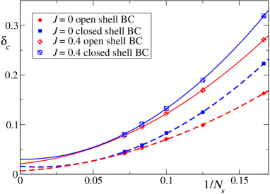
In Fig. 4 we analyze the dependence on size and boundary conditions, for the transition between the Néel and BOW phases determined from the jump in . The finite-size effects are rather large. For and large , the model is equivalent to a spin SU(2) invariant Heisenberg model with alternating bond interactions eric , and from results on the latter model cros ; okam one knows that a spin gap proportional to opens for small . Since the opening of a spin gap indicates a crossing of excited levels and a jump in the spin Berry phase to zero gs , one expects that in the thermodynamic limit, de value of at the transition . If one estimates the error in from the difference between the extrapolated results for open- and closed-shell BC, the result for is consistent with the expected result . Instead, for the extrapolated results for (0.021 for OSBC and 0.030 for CSBC) suggest a small positive extrapolated value. To obtain more precise values of for small , larger system sizes are needed.
VI.3 Pumping circuits
When both and are different from zero, all inversion symmetries are lost and most position expectation values lose their topological protection, except the spin one ,which in absence of a staggered magnetic field, is protected by spin rotation symmetry of around an axis perpendicular to the one. To get further insight into the position expectation values and their related topological invariants we have studied two pumping cycles of the form
| (25) |
where changes from to , in the IRMM with . The corresponding amount of electrons transported in the cycle is expected to be
| (26) |
Multiplying this by the electronic charge , one has the corresponding charge transport [see Eqs. (12) and (13)]. We discuss below some subtleties related with in the analysis of the numerical results.
We take as the unit of energy, OSBC and . The results are very similar for other system sizes except for some details pointed out below.

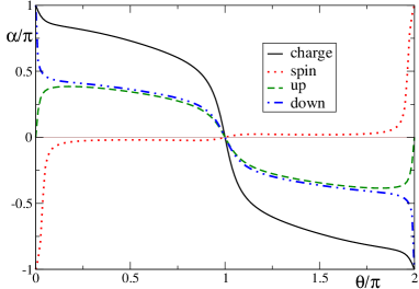
For the first cycle, illustrated in Fig. 5, we take , and . For the chosen parameters and , the critical values of for the charge and spin transition of the IHM lie at . Then for and the system is in the BI phase of the IHM, with site occupancies near 2020… for sites 0,1,2,3 … in the first case and 0202… in the second one. As changes in the interval , with positive , the hopping between sites 0 and 1, 2 and 3, etc. is smaller in magnitude than that between 1 and 2, 3 and 4, etc. Therefore, as changes from negative to positive values, the charges at the even sites displace towards the odd sites moving to the left, taking advantage of the larger magnitude of the hopping. In the remaining part of the cycle, changes sign and the particles continue displacing to the left from the odd sites to the even ones, to reach positions equivalent to the original one. This physical picture explains the results displayed in Fig. 5.
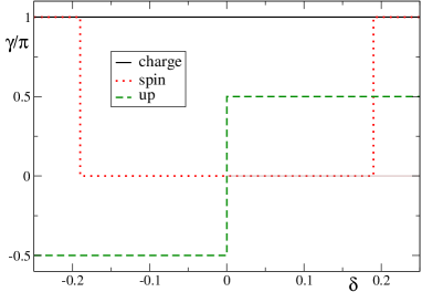
The results for spin up and down are the same. The physics in essentially the same as in the non-interacting RMM and for each spin, an electron is transported around the cycle. Note that for and , as expected in the BI phase of the IHM. Also for all due to the presence of a spin gap. For (), vanishes, the system is described by the ISSHM model with symmetry protected , and () in agreement with Eqs. (24). For an even number of sites not multiple of four (odd ), have almost the same dependence on but are shifted in , as expected from Eqs. (24).
Note that in the whole cycle , and , so that in this case, both contain the whole information. The same happens in the general case in the presence of a staggered field (shown below) which isolates the ground state from the remaining states breaking the degeneracies for all parameters eric .
In the second cycle considered, corresponding to Fig. 6 we take , and . For , we obtain . Then for the system is in the MI phase of the IHM, while for , the system is in the BI phase of the model. We have added first a staggered magnetic field [see Eq. (22)], which simplifies the qualitative analysis in terms of quasi localized charges (that would correspond to small hopping amplitudes). For , the dominant configuration is … for sites 0,1,2,3 … while for the dominant configuration is 0202… Since in the interval , the hopping between sites 1 and 2, 3 and 4, etc is more favorable than the remaining ones, as increases, the electrons with spin down move to the left from the even to the odd sites. In the remaining part of the cycle , also the electrons with spin down move from the doubly occupied odd sites to the left reproducing the original configuration.
The evolution of the different expectation values for this case is shown in Fig. 6. They are topologically protected by inversion symmetry at each site only for and , where they have the value either 0 or . In agreement with the argument above, at the end of the cycle, an electron with spin down is pumped one unit cell to the left, while no net transport takes place for spin up. However, for small staggered field , the difference between both spins is only important near the MI phase (small mod ). For other values of , are qualitatively similar but of smaller magnitude, as the result for the previous cycle. As before, for an even number of sites not multiple of four, are shifted in . We note that if pure spin pumping without charge pumping is wished, one can change the cycle to that of the shape of an eight eric or changing the staggered field in the limit of large shin . In this limit, the model is equivalent to a Heisenberg model with alternating Heisenberg interaction eric with a staggered magnetic field, in which spin pumping is possible shin and similar to the effective model that corresponds to an experimental implementation of a spin pump with ultracold bosonic atoms in an optical superlattice schw2 .
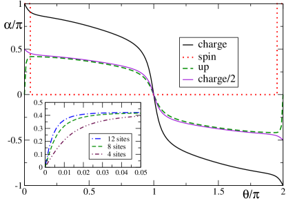
In Fig. 7 we present the different position expectation values for the IRMM with , restoring spin SU(2) symmetry. For , one has (as already displayed in Figs. 1 and 2), therefore, as in Fig. 6, the critical points lie inside the cycle given by Eq. (25). For both figures, the results for and are consistent with previous results, including time-dependent calculations of the charge transport eric indicating that a total of one charge (and no spin in this case) is transported in the cycle. Instead, in this case with , the results for predict no charge transport in contradiction to the previous results. Note that is very near except near the MI phase near 0 mod for which important finite-size effects occur. In fact, as discussed in Section VI.2 for , is expected to be 0 for any and the value near is also a finite-size effect eric .
The size dependence suggests that in the thermodynamic limit and half an electron with spin is transported in the cycle from to with . For , as the system passes through the MI phase (), there is a transition between the two possible BOW phases eric (or spin dimerized phases for large eric ; tzeng ). The BOW order parameter is singular:
| (27) |
This explains the discontinuity in in the thermodynamic limit. As a consequence, Eq. (26) for which assumes a non-degenerate smooth ground state fails for for a path that passes through . For a finite system, there is no singularity at , but the inversion symmetry imposes that should be either 0 or leading to large finite-size effects, that are apparent in Fig. 7. Instead, is continuous and well behaved near . Summarizing these results, one electron is transported in the cycle, in agreement with previous time-dependent calculations eric and half of it corresponds to each spin.
We have also studied the effect of adding a Zeeman term [see Eq. (22)] to the results shown in Fig. 7. The results are qualitatively very similar and therefore are not shown. However, in this case, we expect that in the thermodynamic limit for small (implying small ) there is a spontaneous symmetry breaking between the Néel and anti-Néel states, and the behavior of the would be similar to that shown in Fig. 6 but with .
VII Summary and discussion
We have studied the general properties of topological invariants based on position operators of the form of Eqs. (1) and (2). For the expectation values to be well defined, should be integers, and in some cases different from . In addition, Eq. (17) should be satisfied.
In general, gives the same information as the corresponding Berry phase, except for the sign and quantitative but not qualitative differences due to finite-size effects. In some cases, there is a shift between both quantities, but the changes in polarization coincide except for finite-size effects. For small systems, the jumps in Berry phases provide more accurate results for topological transitions, but the are easier to calculate, and using different boundary conditions an accurate extrapolation to the thermodynamic limit can be obtained. In addition, open boundary conditions can be used li and the formalism can be extended to finite temperature unan .
For the interacting Rice-Mele model, , , give complementary information and using all of them, one can determine the different topological sectors of the model and construct the different phase diagrams. For some parameters, the model reduces to the ionic Hubbard model (IHM) and for others to the interacting Su-Schrieffer-Heeger model (ISSHM). In both cases, the are topological numbers protected by different inversion symmetries. For the case of the IHM, and are enough to determine the phase transitions, while does not show any jumps. The spin transition converges faster to the thermodynamic limit if closed shell boundary conditions (antiperiodic for a number of sites multiple of 4, periodic for even not multiple of 4) are used. For the ISSHM including Ising spin-spin interactions, the jumps in (which can take the values 0 or mod ) and (which can take the values mod ) identify the phase transitions, while is featureless.
The pump cycles shown in Section VI.3 revel subtle finite-size effects in near vanishing hopping alternation. They are related with closing gaps in the thermodynamic limit.
Our study was limited to SU(2) symmetry in the spin sector and one dimension but it can be generalized to SU(N) systems, like half-filled two-orbital ones capp and others osta , and more dimensions. In addition, more information can be extracted using the cumulants of the topological indicators cum0 ; cum1 ; cum ; het1 ; het2
Acknowledgments
We thank E. Bertok and F. Heidrich-Meisner for useful discussions. We acknowledge financial support provided by PICT 2017-2726 and PICT 2018-01546 of the ANPCyT, Argentina.
References
- (1) L. D. Landau and E. Lifshitz, Statistical Physics, (Course of Theoretical Physics, Volume 5) (Butterworth-Heinemann, 1980).
- (2) A. P. Schnyder, S. Ryu, A. Furusaki, and A. W. W. Ludwig, Classification of topological insulators and superconductors in three spatial dimensions Phys. Rev. B 78, 195125 (2008).
- (3) A. Kitaev, Periodic table for topological insulators and superconductors, AIP Conf. Proc. 1134, 22 (2009).
- (4) M. Z. Hasan and C. L. Kane, Topological Insulators, Rev. Mod. Phys. 82, 3045 (2010).
- (5) R-J. Slager, A. Mesaros, V. Juriǐć, and J. Zaanen The space group classification of topological band-insulators, Nat. Physics 9, 98 (2013).
- (6) Y. Ando, Topological Insulator Materials, J. Phys. Soc. Jpn. 82, 102001 (2013).
- (7) C.-K. Chiu, J. C. Y. Teo, A. P. Schnyder, and S. Ryu, Classification of topological quantum matter with symmetries, Rev. Mod. Phys. 88, 035005 (2016).
- (8) B. Bradlyn, L. Elcoro, J. Cano, M. G. Vergniory, Z. Wang, C. Felser, M. I. Aroyo, and B. A. Bernevig, Topological quantum chemistry, Nature 547, 298 (2017).
- (9) J. Kruthoff, Jan de Boer, J. van Wezel, C. L. Kane, and R-J. Slager, Topological Classification of Crystalline Insulators through Band Structure Combinatorics, Phys. Rev. X 7, 041069 (2017).
- (10) J. Wang and S-C. Zhang Topological sates of condensed matter, Nature Mat. 16, 1062 (2017).
- (11) A. Montorsi, F. Dolcini, R. C. Iotti, and F. Rossi, Symmetry-protected topological phases of one-dimensional interacting fermions with spin-charge separation, Phys. Rev. B 95, 245108 (2017).
- (12) V. Gurarie, Single-particle Green’s functions and interacting topological insulators, Phys. Rev. B 83, 085426 (2011).
- (13) S. R. Manmana, A. M. Essin, R. M. Noack, and V. Gurarie, Topological invariants and interacting one-dimensional fermionic systems, Phys. Rev. B 86, 205119 (2012).
- (14) R. Unanyan, M. Kiefer-Emmanouilidis, and M. Fleischhauer, Finite-Temperature Topological Invariant for Interacting Systems, Phys. Rev. Lett. 125, 215701 (2020).
- (15) A. Montorsi, U. Bhattacharya, Daniel González-Cuadra, M. Lewenstein, G. Palumbo, and L. Barbiero, Interacting second-order topological insulators in one-dimensional fermions with correlated hopping, arXiv:2208.00939
- (16) B. Ostahie, D. Sticlet, C. P. Moca, B. Dóra, M. A. Werner, J. K. Asbóth, and G, Zaránd, Multiparticle quantum walk in the strongly interacting SU(3) Su-Schrieffer-Heeger-Hubbard topological model, arXiv:2209.03569
- (17) R. Žitko, G. G. Blesio, L. O. Manuel and A. A. Aligia, Iron phthalocyanine on Au(111) is a “non-Landau” Fermi liquid, Nature Commun. 12, 6027 (2021).
- (18) J. Zak, Berry’s phase for energy bands in solids, Phys. Rev. Lett. 62, 2747 (1989).
- (19) S. Tewari and J. D. Sau, Topological Invariants for Spin-Orbit Coupled Superconductor Nanowires, Phys. Rev. Lett. 109, 150408 (2012).
- (20) J.K. Asbóth, L. Oroszlány, and A. Pályi, A short course on topological insulators, Lecture Notes in Physics, 2016. ISSN 1616-6361. doi: 10.1007/978-3-319-25607-8.
- (21) F. Cardano, A. D’Errico, A. Dauphin, M. Maffei, B. Piccirillo, C. de Lisio, G. De Filippis, V. Cataudella, E. Santamato, L. Marrucci, M. Lewenstein, and P. Massignan, Detection of Zak phases and topological invariants in a chiral quantum walk of twisted photons, Nat. Commun. 8, 15516 (2017).
- (22) D. Pérez Daroca and A. A. Aligia Phase diagram of a model for topological superconducting wires, Phys. Rev. B 104, 115125 (2021).
- (23) R. Resta, Macroscopic polarization in crystalline dielectrics: the geometric phase approach. Rev. Mod. Phys. 66, 899 (1994).
- (24) D. Xiao, M.-C. Chang, and Q. Niu, Berry phase effects on electronic properties, Rev. Mod. Phys. 82, 1959 (2010).
- (25) D. Vanderbilt, Berry Phases in Electronic Structure Theory: Electric Polarization, Orbital Magnetization and Topological Insulators, (Cambridge University Press, 2018).
- (26) B. Bradlyn, and M. Iraola, Lecture notes on Berry phases and topology, SciPost Phys. Lect. Notes 51 (2022).
- (27) G. Ortiz and R. M. Martin, Macroscopic polarization as a geometric quantum phase: Many-body formulation, Phys. Rev. B 49, 14202 (1994).
- (28) R. Resta and S. Sorella, Many-Body Effects on Polarization and Dynamical Charges in a Partly Covalent Polar Insulator, Phys. Rev. Lett. 74, 4738 (1995).
- (29) G. Ortiz, P. Ordejón, R. M. Martin, and G. Chiappe, Quantum phase transitions involving a change in polarization, Phys. Rev. B 54, 13515 (1996).
- (30) X-Y. Song, Y-C. He, A. Vishwanath, and C. Wang, Electric polarization as a nonquantized topological response and boundary Luttinger theorem, Phys. Rev. Research 3, 023011 (2021).
- (31) W. A. Wheeler, L. K. Wagner, and T. L. Hughes Many-body electric multipole operators in extended systems, Phys. Rev. B 100, 245135 (2019).
- (32) M. Tahir and H.Chen, Current-induced quasiparticle magnetic multipole moments, arXiv:2210.15753.
- (33) A. A. Aligia, Berry phases in superconducting transitions, Europhys. Lett. 45, 411 (1999).
- (34) A. A. Aligia, K. Hallberg, C.D. Batista and G. Ortiz, Phase diagrams from topological transitions: The Hubbard chain with correlated hopping, Phys. Rev. B 61, 7883 (2000).
- (35) M.E. Torio, A.A. Aligia, K. Hallberg and H.A. Ceccatto, Phase diagram of the extended Hubbard chain with charge-dipole interactions, Phys. Rev. B 62, 6991 (2000)
- (36) M. E. Torio, A. A. Aligia, and H. A. Ceccatto, Phase diagram of the Hubbard chain with two atoms per cell, Phys. Rev. B 64, 121105(R) (2001).
- (37) M. E. Torio, A. A. Aligia, and H. A. Ceccatto, Phase diagram of the chain at half filling, Phys. Rev. B 67, 165102 (2003) (6 pages)
- (38) K. Nomura and K. Okamoto, Critical properties of S= 1/2 antiferromagnetic XXZ chain with next-nearest-neighbour interactions, J. Phys. A 27, 5773 (1994).
- (39) M. Nakamura, K. Nomura, and A. Kitazawa, Renormalization Group Analysis of the Spin-Gap Phase in the One-Dimensional Model, Phys. Rev. Lett. 79, 3214 (1997).
- (40) M. Nakamura, Mechanism of CDW-SDW Transition in One Dimension, J. Phys. Soc. Jpn. 68, 3123 (1999).
- (41) M. Nakamura, Tricritical behavior in the extended Hubbard chains, Phys. Rev. B 61, 16377 (2000).
- (42) R. D. Somma and A. A. Aligia, Phase diagram of the XXZ chain with next-nearest-neighbor interactions, Phys. Rev. B 64, 024410 (2001).
- (43) G. I. Japaridze and A. P. Kampf, Weak-coupling phase diagram of the extended Hubbard model with correlated-hopping interaction, Phys. Rev. B 59, 12822 (1999).
- (44) A. A. Aligia and L. Arrachea, Triplet superconductivity in quasi-one-dimensional systems Phys. Rev. B 60, 15332 (1999).
- (45) R. Resta, Quantum-Mechanical Position Operator in Extended Systems, Phys. Rev. Lett. 80, 1800 (1998).
- (46) R. Resta and S. Sorella, Electron Localization in the Insulating State, Phys. Rev. Lett. 82, 370 (1999).
- (47) A. A. Aligia and G. Ortiz, Quantum Mechanical Position Operator and Localization in Extended Systems, Phys. Rev. Lett. 82, 2560 (1999).
- (48) G. Ortiz and A. A. Aligia, How localized is an extended quantum system ?, Phys. Status Solidi B 220, 737 (2000).
- (49) M. Nakamura and S. Todo, Order Parameter to Characterize Valence-Bond-Solid States in Quantum Spin Chains Phys. Rev. Lett. 89, 077204 (2002).
- (50) C. D. Batista, G. Ortiz, and A. A. Aligia, Ferrotoroidic Moment as a Quantum Geometric Phase, Phys. Rev. Lett. 101, 077203 (2008).
- (51) I. Souza, T. Wilkens, and R. M. Martin, Polarization and localization in insulators: Generating function approach, Phys. Rev. B 62, 1666 (2000).
- (52) G. Ortiz and A. A. Aligia, How Localized is an Extended Quantum System? Physica Status Solidi (b) 220, 737 (2000).
- (53) B. Hetényi and B. Dóra, Quantum phase transitions from analysis of the polarization amplitude, Phys. Rev. B 99, 085126 (2019).
- (54) B. Hetényi, Interaction-driven polarization shift in the lattice fermion model at half filling: Emergent Haldane phase, Phys. Rev. Research 2, 023277 (2020).
- (55) B. Hetényi and S. Cengiz, Geometric cumulants associated with adiabatic cycles crossing degeneracy points: Application to finite size scaling of metal-insulator transitions in crystalline electronic systems, Phys. Rev. B 106, 195151 (2022).
- (56) B. Hetényi, S. Parlak, and M. Yahyavi, Scaling and renormalization in the modern theory of polarization: Application to disordered systems, Phys. Rev. B 104, 214207 (2021)
- (57) D. J. Thouless, Quantization of particle transport, Phys. Rev. B 27, 6083 (1983).
- (58) Q. Niu and D. J. Thouless, Quantised adiabatic charge transport in the presence of substrate disorder and many-body interaction, J. Phys. A: Math. Gen. 17, 2453 (1984).
- (59) S. Nakajima, T. Tomita, S. Taie, T. Ichinose, H. Ozawa, L. Wang, M. Troyer, and Y. Takahashi, Topological Thouless pumping of ultracold fermions, Nat. Phys. 12, 296 (2016).
- (60) M. Lohse, C. Schweizer, O. Zilberberg, M. Aidelsburger, and I. Bloch, A Thouless quantum pump with ultracold bosonic atoms in an optical superlattice Nat. Phys. 12, 350 (2016).
- (61) M. J. Rice and E. J. Mele, Elementary Excitations of a Linearly Conjugated Diatomic Polymer, Phys. Rev. Lett. 49, 1455 (1982).
- (62) C. Schweizer, M. Lohse, R. Citro, and I. Bloch, Spin Pumping and Measurement of Spin Currents in Optical Superlattices, Phys. Rev. Lett. 117, 170405 (2016).
- (63) A.-S. Walter, Z. Zhu, M. Gächter, J. Minguzzi, S. Roschinski, K. Sandholzer, K. Viebahn, and T. Esslinger, Breakdown of quantisation in a Hubbard-Thouless pump arXiv:2204.06561.
- (64) M. Nakagawa, T. Yoshida, R. Peters, and N. Kawakami, Breakdown of topological Thouless pumping in the strongly interacting regime, Phys. Rev. B 98, 115147 (2018).
- (65) L. Stenzel, A. L. C. Hayward, C. Hubig, U. Schollwöck, and F. Heidrich-Meisner, Quantum phases and topological properties of interacting fermions in one-dimensional superlattices, Phys. Rev. A 99, 053614 (2019).
- (66) E. Bertok, F. Heidrich-Meisner, and A. A. Aligia, Splitting of topological charge pumping in an interacting two-component fermionic Rice-Mele Hubbard model, Phys. Rev. B 106, 045141 (2022).
- (67) R. Citro and M. Aidelsburger, Thouless pumping and topology, arXiv:2210.02050, Nature Reviews Physics (2023) DOI: 10.1038/s42254-022-00545-0.
- (68) W. P. Su, J. R. Schrieffer, and A. J. Heeger, Solitons in Polyacetylene, Phys. Rev. Lett. 42, 1698 (1979).
- (69) P. Molignini and N. Cooper, Topological phase transitions at finite temperature, arXiv:2208.08994
- (70) R. Li and M. Fleischhauer, Finite-size corrections to quantized particle transport in topological charge pumps, Phys. Rev. B 96, 085444 (2017).
- (71) M. Fabrizio, A.O. Gogolin, and A.A. Nersesyan, From Band Insulator to Mott Insulator in One Dimension, Phys. Rev. Lett. 83, 2014 (1999).
- (72) S. R. Manmana, V. Meden, R. M. Noack, and K. Schönhammer, Quantum critical behavior of the one-dimensional ionic Hubbard model, Phys. Rev. B 70, 155115 (2004).
- (73) M. E. Torio, A. A. Aligia, G. I. Japaridze, and B. Normand, Quantum phase diagram of the generalized ionic Hubbard model for ABn chains, Phys. Rev. B 73, 115109 (2006)
- (74) A. A. Aligia, Charge dynamics in the Mott insulating phase of the ionic Hubbard model, Phys. Rev. B 69, 041101(R) (2004).
- (75) C. Lanczos, An iteration method for the solution of the eigenvalue problem of linear differential and integral operators, J. Res. Nat. Bur. Std. 45, 225 (1950).
- (76) R. Kobayashi, Y. O. Nakagawa, Y. Fukusumi, and M. Oshikawa, Scaling of the polarization amplitude in quantum many-body systems in one dimension Phys. Rev. B 97, 165133 (2018).
- (77) Y.-C. Tzeng, L. Dai, M.-C. Chung, L. Amico, and L.-C. Kwek, Entanglement convertibility by sweeping through the quantum phases of the alternating bonds XXZ chain, Sci. Rep. 6, 26453 (2016).
- (78) M. C. Cross and D. S. Fisher, A new theory of the spin-Peierls transition with special relevance to the experiments on TTFCuBDT, Phys. Rev. B 19, 402 (1979).
- (79) K. Okamoto, H. Nishimori, and Y. Taguchi, A numerical study of spin-1/2 alternating antiferromagnetic Heisenberg linear chains, J. Phys. Soc. Jpn. 55, 1458 (1986).
- (80) R. Shindou, Quantum Spin Pump in S=1/2 Antiferromagnetic Chains –Holonomy of Phase Operators in sine-Gordon Theory, J. Phys. Soc. Jpn. 74, 1214 (2005).
- (81) V. Bois, S. Capponi, P. Lecheminant, M. Moliner, and K. Totsuka, Phys. Rev. B 91, 075121 (2015).