A Comprehensive Survey of Data Augmentation
in Visual Reinforcement Learning

Abstract

Visual reinforcement learning (RL), which makes decisions directly from high-dimensional visual inputs, has demonstrated significant potential in various domains. However, deploying visual RL techniques in the real world remains challenging due to their low sample efficiency and large generalization gaps. To tackle these obstacles, data augmentation (DA) has become a widely used technique in visual RL for acquiring sample-efficient and generalizable policies by diversifying the training data. This survey aims to provide a timely and essential review of DA techniques in visual RL in recognition of the thriving development in this field. In particular, we propose a unified framework for analyzing visual RL and understanding the role of DA in it. We then present a principled taxonomy of the existing augmentation techniques used in visual RL and conduct an in-depth discussion on how to better leverage augmented data in different scenarios. Moreover, we report a systematic empirical evaluation of DA-based techniques in visual RL and conclude by highlighting the directions for future research. As the first comprehensive survey of DA in visual RL, this work is expected to offer valuable guidance to this emerging field. A well-classified paper list that will be continuously updated can be found at this GitHub site.

1 Introduction

Reinforcement learning (RL) addresses sequential decision making problems in which an agent seeks to discover the optimal policy via trial-and-error interactions with the environment [1, 2, 3, 4]. Since visual observations such as images are intuitive and cost-effective for an agent to perceive its environment [5, 6], visual RL learning from visual observations has been widely applied in various domains, including video games [7], autonomous driving [8], robot control [9], etc. However, learning directly from high-dimensional visual observations is still largely hindered by the challenges of low sample efficiency and large generalization gaps [10, 11, 6, 12, 13, 14, 15].

To learn sample-efficient and generalizable visual RL agents, a considerable amount of effort has been devoted to developing diverse approaches, including $(1)$ applying explicit regularization techniques such as entropy regularization [16, 17] to constrain the model’s weights [18, 19, 20]; $(2)$ performing joint learning with RL loss and auxiliary tasks to provide additional representation supervision [6, 21, 22, 23, 24, 25, 26, 27, 28, 29, 30, 31, 32, 33, 34]; $(3)$ building a world model of the RL environment that allows learning behaviors from imagined outcomes [35, 36, 37, 11]; and $(4)$ pretraining an encoder that can project high-dimensional observations into compact state representation [38, 39, 40, 41, 42, 43, 44, 45, 46, 47].

Although these approaches have achieved remarkable success, they are still challenged by limited interaction data and poor sample diversity [12, 13, 14]. To increase the quantity and diversity of the training data, data augmentation (DA) has received increasing attention from the visual RL community in recent years [13, 14, 15, 23, 48]. As a data-driven method, DA is orthogonal to the aforementioned methods and can be combined with them to further improve the performance [23, 49]. For example, DA plays a crucial role in contrastive-based auxiliary tasks to inject the prior knowledge of task invariance [26, 38, 50]. In addition, DA is essential for pre-training a cross-task representation [38, 39]. Furthermore, various DA techniques such as random cropping have been used in almost all visual RL algorithms as a form of data preprocessing [37, 31, 5].

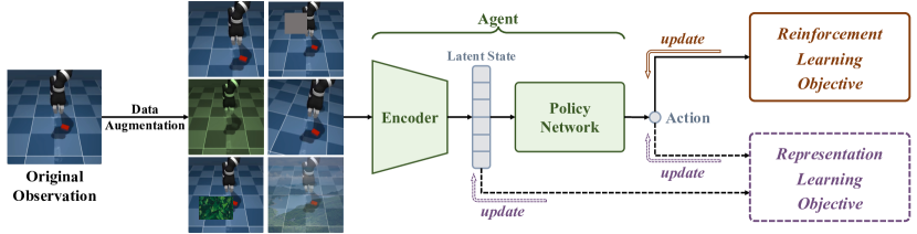
Figure 1: The generic workflow diagram for leveraging DA in visual RL.

In general, DA refers to the strategies for generating synthetic training data from existing data without additional collection or interaction efforts [51, 52]. Figure 1 shows the generic workflow for leveraging DA in visual RL: diverse augmented data are generated by manipulating the original interaction data and then exploited to optimize the RL objective [12, 13, 14]. Moreover, DA can further improve the representation of visual RL by optimizing auxiliary representation learning objectives [53, 54, 26, 23]. Despite the surge of these related studies on leveraging DA in visual RL scenarios, this fast-evolving and expanding field still lacks clarity and coherence. Therefore, this comprehensive survey aims to provide a bird’s eye view of DA-based methods in visual RL with the following main contributions.

1. Based on previous works [55, 56], we present HCMDP as a general framework to formalize visual RL and gain deep insights into the challenges of low sample efficiency and large generalization gaps in visual RL.

2. We identify two key assumptions of DA with different motivations: the optimality invariance assumption for improving sample efficiency and the prior-based diversity assumption for narrowing the generalization gap.

3. We categorize related techniques from two principled perspectives: how to augment data and how to leverage augmented data for improved clarity and coherence.

4. We conduct a unified empirical evaluation of extensive DA-based methods on representative benchmarks to evaluate their sample efficiency and generalization abilities.

5. We present an in-depth discussion of the critical issues faced by DA in visual RL to highlight the specific challenges and future directions in this filed.

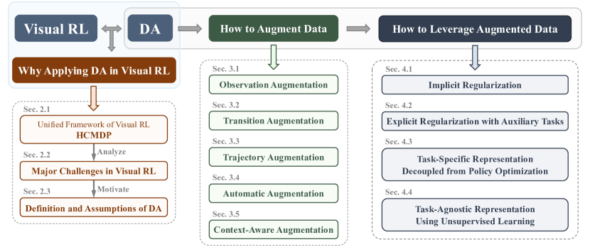
Figure 2: The schematic structure of this survey.

The body of this survey is organized as Figure 2. In Section 2, we propose a unified high-dimensional contextual Markov decision process (HCMDP) framework (Section 2.1) to formalize the visual RL scenario and highlight its major challenges (Section 2.2), as well as present the motivations and definitions of DA in visual RL (Section 2.3). We then conduct a systematic review of the previous work from two perspectives: how to obtain and how to leverage augmented data in visual RL (Section 3 and Section 4). In Section 3, we divide the DA approaches in visual RL into observation augmentation, transition augmentation and trajectory augmentation, depending on the type of data that a DA technique aims to modify. Moreover, we introduce automatic augmentation and context-aware augmentation as two extensions. In Section 4, we present the different mechanisms used to leverage DA in visual RL, including implicit and explicit regularization, task-specific representation learning decoupled from policy optimization, and task-agnostic representation learning using unsupervised learning. To reveal the practical effect of DA, we introduce the typical benchmarks and summarize the empirical performance of recent DA-based methods in Section 5. In Section 6, we put forward a critical discussion concerning future research directions, including the opportunities, challenges, limitations, and theoretical guarantees of DA. Finally, this survey is concluded in Section 7 with a list of key insights.

Note that this survey focuses on the scenarios that involve learning directly from visual inputs instead of handcrafted state inputs. In addition, this survey does not cover a somewhat related topic named domain randomization (DR) [57, 58], which aims to solve the sim-to-real problem in robot control by tuning the physical simulator’s parameter distribution toward the reality as closely as possible [59]. By contrast, DA can only manipulate observations after rendering while the access to the simulator’s internal parameters is unavailable [55].

2 Preliminaries

Visual RL addresses high-dimensional image observations instead of well-designed states and has encountered a series of new challenges [6, 13]. This section analyzes visual RL in depth and introduces the formalism of DA used for visual RL. In Section 2.1, we present a novel framework, HCMDP, to formalize the paradigm of visual RL. Based on this framework, we analyze the major challenges faced by visual RL in Section 2.2. Finally, Section 2.3 introduces the formalism of DA in visual RL, including its motivation, definition and two key assumptions.

2.1 High-Dimensional Contextual MDP (HCMDP)

The standard RL task is often defined as a Markov Decision Process (MDP) [2], which is specified by a tuple $\mathcal{M}=(\mathcal{S},\mathcal{A},r,\mathcal{P},p,\mathcal{\gamma})$ where $\mathcal{S}$ is the state space; $\mathcal{A}$ is the action space; $r:\mathcal{S}\times\mathcal{A}\times\mathcal{S}\mapsto\mathbb{R}$ is the scalar reward function; $\mathcal{P}(s^{\prime}|s,a)$ is the transition function; $p(\cdot)$ is the initial state distribution; and $\gamma\in(0,1]$ is the discount factor. The goal of RL is to learn an optimal policy $\pi^{*}(a\mid s)$ that maximizes the expected cumulative discounted return $\mathcal{R}(\pi,\mathcal{M})$, which is defined as:

$$\mathcal{R}(\pi,\mathcal{M})=\mathbb{E}_{{s_{o}\sim p(\cdot)},{a_{t}\sim\pi\left(\cdot\mid s_{t}\right)},{s_{t+1}\sim\mathcal{P}(\cdot\mid s_{t},a_{t})}}\left[\sum_{t=0}^{\infty}\gamma^{t}r\left(s_{t},a_{t},s_{t+1}\right)\right]$$ (1)

Although the MDP is the standard paradigm of RL, it ignores a crucial factor of visual RL: agents only have direct access to high-dimensional observations instead of the actual state information. To properly formulate the visual RL scenarios, as shown in Figure 3, many variants of MDPs [60, 61, 62, 63] have been introduced by using the high-dimensional observation space $\mathcal{O}$ to represent the image inputs. Depending on the specific assumptions, an emission function $\phi:\mathcal{S}\mapsto\mathcal{O}$ can be designed to simulate the mapping from the state space $\mathcal{S}$ to the observation space $\mathcal{O}$. For example, the $(f,g)$-scheme [56] constructs an emission function as the combination of generalizable and non-generalizable features while the contextual MDP (CMDP) [64, 63, 65, 55] introduces context $c$ to distinguish contextual information from the underlying state information. However, these MDP variants mainly focus on how to explain the generalization effect in visual RL, and ignore the issue of constructing a compact representation from high-dimensional observations.

To better understand visual RL scenarios and provide a unified view of its specific challenges, we propose High-Dimensional Contextual MDP (HCMDP) as a general modeling framework of visual RL. Following the previous formalism [55, 56], the HCMDP $\mathcal{M}|_{C}$ can be defined as a family of environments:

$$\mathcal{M}|_{C}=\{\mathcal{M}|_{c}=(\mathcal{M},\mathcal{O}_{c},{\phi}_{c})\mid c\sim p(c),c\in C\}$$ (2)

where $\mathcal{M}=(\mathcal{S},\mathcal{A},r,\mathcal{P},p,\mathcal{\gamma})$ specifies the dynamics of the underlying system. With the fixed base MDP $\mathcal{M}$, the observation space $\mathcal{O}_{c}$ and emission function ${\phi}_{c}$ depend on the context $c$, which refers to the peripheral parameters that are not essential for agents to make decisions. $p(c)$ is the context distribution, and $C$ represents the entire context set. For example, the colors and styles of backgrounds in robot scenarios are extraneous to control tasks, and are thus being referred to as task-irrelevant features.

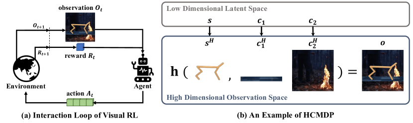
Figure 3: The agent-environment interaction loop of visual RL and an example of HCMDP.

To be more specific, context $c$ can be denoted as a set of parameters $\{c_{1},c_{2},\dots,c_{n}\}$, where $n$ is the number of task-irrelevant properties in this system. Each $c_{i}$ corresponds to a task-irrelevant property, all of which are distributed over a fixed range: $\left\{c_{1}\in C_{1},c_{2}\in C_{2},\ldots,c_{n}\in C_{n}\right\}$. Consider an autonomous driving example such as CARLA [66]: an agent learns to control the car directly from pixels in changing environments. Therefore, the agent must distinguish between task-relevant and task-irrelevant components in the image observations. For instance, we can denote the style of the background buildings as $c_{1}$, the color of the driving car as $c_{2}$ and the number of people walking on the sides of the road as $c_{3}$.

The state $s$ and context $c$ constitute the complete information (parameters) used by the system to render the final observed images [56]. However, they both exist in the low-dimensional latent space, which cannot be directly observed. In fact, $\mathcal{O}$ is the only observable high-dimensional space where agents perceive task information. Following the assumptions [65, 56] that observations are high-dimensional projections of the state $s$ and task-irrelevant contexts $c$, the emission function $\phi_{c}$ mapping from state $s\in\mathcal{S}$ to observation $o\in\mathcal{O}_{c}$ can be defined as:

$$o=\phi_{c}(s):=\mathbf{h}(s^{H},c_{1}^{H},c_{2}^{H},\dots,c_{n}^{H})$$ (3)

where $s^{H}$ is the high-dimensional representation mapped from the underlying state $s$, and each $c_{i}^{H}$ is the high-dimensional representation uniquely determined by the latent context $c_{i}$. Similar to the formalism in [56], $\mathbf{h}$ is a "combination" function that combines the task-relevant state representation $s^{H}$ and task-irrelevant context representations $(c_{1}^{H},c_{2}^{H},\dots,c_{n}^{H})$ to render the final observation. Based on the HCMDP framework, Figure 3 shows an illustration of a robot control environment from the DeepMind control suite [10]. In this scenario, contexts $c_{1}$ and $c_{2}$ separately denote the floor color and background style, respectively, which are both irrelevant to the control task. Correspondingly, $c_{1}^{H}$ and $c_{2}^{H}$ are the high-dimensional representations mapped from $c_{1}$ and $c_{2}$. The final observation $o$ is the combination of the state representation $s^{H}$ and the task-irrelevant representations $c_{1}^{H}$ and $c_{2}^{H}$.

An HCMDP $\mathcal{M}|_{C}$ consists of a family of specific environments, where $c$ follows the context distribution $p(c)$ over the entire context set $C$. In a given system, $\mathcal{M}$ and the rendering rules from $s$ and $c_{i}$ to the high-dimensional representations $s^{H}$ and $c_{i}^{H}$ are established. Hence, different combinations of the context distribution $p(c)$ and context set $C$ produce different HCMDPs. For any HCMDP $\mathcal{M}|_{C}$, the expected return of a policy is defined as:

$$\mathbf{R}(\pi,\mathcal{M}|_{C}):=\mathbb{E}_{c\sim p(c),c\in C}\left[\mathcal{R}\left(\pi,\mathcal{M}|_{c}\right)\right]$$ (4)

where $\mathcal{R}$ is the expected return of policy $\pi$ in a specific MDP. In practice, we assume that the context distribution is uniform over the entire context set [55] so that different HCMDPs can be specified by their context sets $C=(C_{1},C_{2},\dots,C_{n})$. By choosing a training context set $C_{\rm train}$ and a test context set $C_{\rm test}$, we can separately define the training context set HCMDP $\mathcal{M}|_{C_{\rm train}}$ and the test context set HCMDP $\mathcal{M}|_{C_{\rm test}}$. Agents are only allowed to be trained in $\mathcal{M}|_{C_{\rm train}}$ and evaluated in the same HCMDP $\mathcal{M}|_{C_{\rm train}}$ or HCMDP $\mathcal{M}|_{C_{\rm test}}$, whose context exhibits a distribution shift from the training context set.

Remarks.

The main difference between HCMDP and other MDP variants lies in the emission function $\phi:\mathcal{S}\mapsto\mathcal{O}$, as shown in Figure 4.

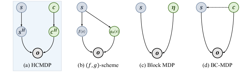
Figure 4: A graphical model of the emission function of a HCMDP (a) compared with three other representative MDP variants: (b) $(f,g)$-scheme [56], (c) Block MDP [67] and (d) BC-MDP [68].

First, the HCMDP highlights the high dimensionality of the observation space $\mathcal{O}$ by explicitly specifying the mapping between the latent variables $s,c$ and their high-dimensional representations $s^{H},c^{H}$. Second, it presents a unified perspective to understand the challenges of generalizing learned policy to unseen visual environments based on existing assumptions [56, 67, 68]. Specifically, the HCMDP assumes that the task-relevant features of state $s$ and the task-irrelevant features of context $c$ are combined in the final observation without further assumptions about their relationship. In the training process, agents tend to overfit the irrelevant context features and cannot effectively generate to unseen environments. As a general framework, the HCMDP can be transformed to other feasible MDP variants by making additional assumptions. For example, $(f,g)$-scheme [56] assumes that the unimportant features that do not contribute to extra generalizable information in observations are projected from the latent state with function $g_{\theta}(\cdot)$ dependent on the sampled parameter $\theta$; Block MDP [67] assumes that the emission function is the concatenation of the noise and state variables as $s\oplus f(\eta)$, where $\eta$ denotes spurious noise; and BC-MDP [68] assumes that the agent only has access to a partial state space $\mathcal{S}^{c}$, determined by the context $c$. By contrast, the HCMDP ignores the specific relationship between task-relevant and task-irrelevant features, focusing instead on the compound of these components.

Note that the HCMDP framework does not take into account the partially observable features of the underlying states in a partially observable MDP (POMDP) [69]. Following [2, 39, 13], we assume that the complete state information can be reasonably constructed by stacking three consecutive previous image observations into a trajectory snippet [14]. In summary, the motivation of HCMDP is to emphasize the fact that the underlying state $s$ is projected to the high-dimensional observation space along with the task-irrelevant information of context $c$. With this unified framework, the unique challenges of visual RL scenarios compared with standard RL can be clearly analyzed.

2.2 Major Challenges in Visual RL

Despite the success of visual RL in complex control tasks with visual observations, sample efficiency and generalization remain two major challenges that may lead to ineffective agents [23, 15, 48, 70, 71]. In this subsection, we present the formal definitions of sample efficiency and the generalization gap based on the HCMDP framework and discuss their mechanisms.

2.2.1 Sample Efficiency

This term measures how well the interaction data are leveraged to train a model [72]. In practice, we consider an agent sample-efficient if it can achieve satisfactory performance within limited environment interactions [13, 23]. In other words, the goal of sample-efficient RL is to maximize the policy’s expected return during the training of HCMDP $\mathcal{M}|_{C_{\rm train}}$ based on as few interactions as possible. The expected return of policy $\pi$ in $\mathcal{M}|_{C_{\rm train}}$ can be defined as:

$$J(\pi):=\mathbf{R}(\pi,\mathcal{M}|_{C_{\rm train}})$$ (5)

Instead of making decisions based on predefined features, agents in visual RL need to learn an appropriate representation that maps a high-dimensional observation $\mathbf{h}(s^{H},c^{H})$ to the latent space $\mathbf{h}(s,c)$ to obtain decision-critical information [23, 13, 12]. Since standard RL algorithms already require large amounts of interaction data [17], learning directly from high-dimensional observations suffers from prohibitive sample complexity [6].

One solution to the sample inefficiency problem in visual RL is by training with auxiliary losses, such as pixel or latent reconstruction [6, 21], future prediction [22, 23, 24, 25] and contrastive learning for instance discrimination [26, 27, 28, 29] or temporal discrimination [73, 30, 31, 32, 33]. Meanwhile, several model-based methods explicitly build a world model of the RL environment in pixel or latent spaces to conduct planning [35, 36, 37, 11]. Recently, pretrained encoders have demonstrated great potential in downstream tasks where the visual RL environment is explored in an unsupervised manner to obtain a task-agnostic pretrained encoder that can quickly adapt to diverse downstream tasks [38, 39, 40, 41]. In addition, applying the pretrained encoders from other domains such as ImageNet [74] to visual RL also has shown its efficiency in downstream tasks [43, 44, 45, 46]. The aforementioned methods have significantly improved the sample efficiency of visual RL, but the lack of training data remains a fundamental issue, which can be effectively solved by DA. Moreover, abundant auxiliary tasks and world models are designed and trained based on the augmented data [26, 23, 24, 11]. Hence, DA plays a vital role in improving the sample efficiency of visual RL algorithms.

2.2.2 Generalization

An agent’s generalization ability can be measured by the generalization gap when transferred to unseen environments, which has been extensively investigated [56, 60, 75] and reviewed [55]. For an HCMDP with varying context sets ${C_{\rm train}}$ and ${C_{\rm test}}$, the generalization gap of policy $\pi$ can be defined as:

$$\mathrm{GenGap}(\pi):=\mathbf{R}(\pi,\mathcal{M}|_{C_{\rm train}})-\mathbf{R}(\pi,\mathcal{M}|_{C_{\rm test}})$$ (6)

As mentioned in Section 2.1, the task-relevant information of state $s$ is often conflated with the task-irrelevant information of context $c$, which may cause agents to overfit the task-irrelevant components [56]. How to train generalizable agents across different environments remains challenging in visual RL, and distinguishing between the task-relevant and task-irrelevant components of the observed images is essential for narrowing the generalization gap.

A naive approach to enhancing generalization is to apply regularization techniques originally developed for supervised learning [18, 19], including $\ell_{2}$ regularization [76], entropy regularization [16, 17], dropout [20] and batch normalization [77]. However, these traditional regularization techniques show limited improvement in generalization and may even negatively impact sample efficiency [18, 13, 77]. As a result, recent studies focus on learning robust representations to improve the agent’s generalization ability by introducing bisimulation metrics [78, 79], multi-view information bottleneck (MIB) [29], pretrained image encoder [42] etc. From an orthogonal perspective, DA has been effective in enhancing generalization by generating diverse synthetic data [12, 13]. Moreover, DA can implicitly provide prior knowledge to the agent as a type of inductive bias or regularization [55, 80]. A detailed elaboration of the generalization issue in RL is provided in [55], which systematically reviews the related studies.

2.3 DA in Visual RL

As discussed in Section 2.2, the quantity and diversity of training data are crucial for achieving sample-efficient and generalizable visual RL algorithms. DA, as a data-driven approach, has demonstrated significant potential for visual RL in terms of both sample efficiency and generalization ability [12, 13, 14, 15, 48, 81, 38, 54]. The advantages of DA for visual RL can be viewed from two aspects: $(1)$ it can significantly expand the volume of the original interaction data, thus improving the sample efficiency [12]; $(2)$ it introduces additional diversity into the original training data, making agents more robust to variations and enhancing their generalization capabilities [55, 15]. Furthermore, theoretical foundations have also been developed for DA, such as invariance learning [82, 83] and feature manipulation [84]. Hence, DA has been well recognized as a viable solution for the challenges in visual RL [85, 55, 15]. Following the conventions in [13, 14, 15], we define a general augmentation $\tau:\mathcal{O}\times\mathcal{V}\mapsto\mathcal{O}^{aug}$ as a mapping from the original observation space $\mathcal{O}$ to the augmented observation space $\mathcal{O}^{aug}$:

$$o^{aug}\triangleq\tau(o;\nu)\qquad\forall o\in\mathcal{O},\nu\in\mathcal{V}$$ (7)

where $\nu\in\mathcal{V}$ is a set of random parameters and $\tau(\cdot)$ is the transformation function acting on the observation $o$. To gain an intuitive understanding of the effect of DA, we identify two assumptions of $\tau(\cdot)$ corresponding to the challenges that DA seeks to address: the assumption of optimality invariance for improving the sample efficiency and the assumption of prior-based diversity for narrowing the generalization gap.

2.3.1 Optimality Invariance

In supervised learning (SL), DA methods usually assume that the model’s output is invariant after transformations; therefore, they can be directly applied to labeled samples to produce supplementary data [51, 86]. Considering the property of RL, DrQ [13] defines the optimality invariance assumption as adding a constraint to the transformation $\tau$, which induces an equivalence relation between state $s$ and its augmented counterpart $s^{aug}$ constructed from observations $o$ and $o^{aug}$, respectively [15]. Hence, an optimality-invariant state transformation $\tau:\mathcal{O}\times\mathcal{V}\mapsto\mathcal{O}$ can be defined as a mapping that preserves the Q-values [15], V-values and policy $\pi$ [54] :

$$Q(o,a)=Q(\tau(o;\nu),a),V(o)=V(\tau(o;\nu))\text{ and }\pi(o)=\pi(\tau(o;\nu))\quad\forall o\in\mathcal{O},a\in\mathcal{A},\nu\in\mathcal{V}$$ (8)

where $\nu$ is the set of parameters of $\tau(\cdot)$, drawn from the set of all possible parameters $\mathcal{V}$. Note that optimality invariance relies on strict restrictions on $\tau(\cdot)$ and the size of $\mathcal{V}$ to ensure that the same $s$ can be constructed from the original and augmented observations. In the HCMDP framework, optimality invariance means that augmentation transformations only change the selected contexts in the high-dimensional observation space while preserving the entire (conceptual) state information in the latent space.

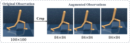
Figure 5: Optimality-Invariant augmentation.

For instance, random cropping [12, 13] satisfies the optimality invariance assumption in most robot control environments such as the DeepMind control suite [10]. In Figure 5, cropping generates augmented observations by randomly extracting central patches from the original image. Since the robot is centrally placed in the images, cropping only eliminates irrelevant information such as the background color while preserving the task-relevant information such as the robot’s posture [65].

With the optimality-invariant augmentation of the original observations, we can obtain sufficient training data based on limited interactions with the environment so that the sample efficiency can be significantly improved [13, 54]. However, due to the constraint of Eq. 8, optimality-invariant augmentations cannot provide sufficient diversity to enhance the agent’s generalization ability [13, 15]. Consequently, it is necessary to break the limitation of optimality invariance to capture the variation between the training and test environments [15, 55].

2.3.2 Prior-Based Diversity

Based on the prior knowledge of the task-irrelevant contexts that vary between the training and test environments, targeted augmentations can be applied to effectively capture these variations [55]. Consequently, prior-based diversity can be introduced by modifying the corresponding features in the observed images. Note that DA can only manipulate the observed images and cannot directly change the distribution of the latent context. Figure 6 shows a typical scenario of DMControl-GB [53]. With the knowledge that the background color and style may vary when transferring the agent from training environments to test environments, we can purposefully employ augmentation techniques such as color jitter to diversify the color of the training observations [15]. By developing an invariant policy or a latent representation from the prior-based strong augmentation (under the prior-based diversity assumption), the agents can successfully learn to identify these task-irrelevant features [55].

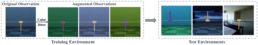
Figure 6: Examples of applying DA under the assumption of prior-based diversity.

Strong augmentation under the prior-based diversity assumption breaks the limitation of the optimality invariance assumption and therefore has tremendous potential for improving the agent’s generalization ability. However, this approach inevitably increases the estimation variance of the Q-values and thus may harm the stability of the RL optimization process [15, 48].

3 How to Augment Data in Visual RL?

The aim of DA is to increase the amount and diversity of the original training data so that agents can learn more efficient and robust policies [15]. Thus, a primary focus of previous research was to design effective augmentation approaches [49, 24]. In this section, we introduce the mainstream augmentation techniques and discuss the pros and cons of these methods.

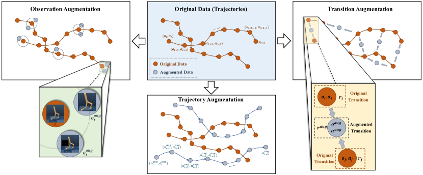
Figure 7: The comparison of different DA paradigms depending on the type of data augmented: observation augmentation only generates synthetic observations $o_{t}^{aug}$; transition augmentation augments observations together with supervision signals $(o_{t}^{aug},a_{t}^{aug},r_{t}^{aug})$; and trajectory augmentation generates virtual trajectories $(o_{t}^{aug},a_{t}^{{aug}},o_{t+1}^{{aug}},a_{t+1}^{aug},\ldots,o_{t+k}^{aug})$.

In Figure 7, we divide the DA approaches in visual RL into three main categories. Observation augmentation only transforms the given observations and keeps the other transition factors (e.g., actions and rewards) unchanged, which is similar to the label-preserving perturbations in SL. This kind of augmentation technique can be further categorized into two groups: classic image manipulations (Section 3.1) and deep neural network (DNN)-based transformations (Section 3.2). The other two augmentation types, transition augmentation and trajectory augmentation, specifically consider the properties of RL to expand the scope of augmentation. In Section 3.3, we introduce transition augmentation, which augments observations along with supervision signals such as rewards. In Section 3.4, we discuss trajectory augmentation for generating synthesized sequential trajectories. Furthermore, we present automatic augmentation (Section 3.5) and task-aware augmentation (Section 3.6) as two extensions that are vital for achieving effective augmentation.

3.1 Observation Augmentation via Classic Image Manipulations

A typical observation augmentation approach is to apply the classical image manipulations to the observed images; most such manipulations were originally proposed for computer vision applications. Following the taxonomy of [51], we identify five categories of image manipulations: geometric transformations (Section 3.1.1), photometric transformations (Section 3.1.2), noise injections (Section 3.1.3), random erasing (Section 3.1.5) and image mixing (Section 3.1.4). Figure 8 shows a list of the visualized examples.

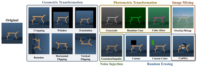
Figure 8: Visualized examples of observation augmentation via classical image manipulations.

3.1.1 Geometric Transformations

Geometric transformations are generally employed as optimality-invariant or label-preserving transformations [51] to overcome data shortages during the training process. Random cropping is an effective preprocessing technique for improving data efficiency; it works on image data with mixed width and height dimensions by locating a random central patch in each frame with a specific dimensionality [13, 14]. In many visual RL scenarios, such as robotic manipulation tasks, the vital regions are often positioned at the centers of the images, and cropping can remove irrelevant edge pixels to simplify the learning process [12]. Similar to cropping, the window transformation selects a random region and masks out the cropped part of the image, while translation renders the image with a larger frame and randomly moves the image within that frame.

Other forms of geometric transformation have also been introduced in visual RL scenarios. For example, rotation involves rotating an image right or left by $r$ degrees, where $r$ is randomly selected from a range [12]; flipping obtains additional data by flipping the observations horizontally or vertically. Although these techniques have been proven effective in computer vision tasks such as ImageNet [51], visual RL tasks are sensitive to angle information. In such a scenario, transformations such as rotation and flipping may produce erroneous results without properly adjusting the corresponding actions.

3.1.2 Photometric Transformations

In real-world applications, the colors of objects and backgrounds may vary due to conditions such as lighting and weather [87]. The intuition behind photometric transformations is to simulate these color variations to prevent overfitting on the training data [88, 89]. Overfitting in visual RL is especially problematic due to the spurious correlations between task-irrelevant features and the agent’s policy, which can severely damage its test performance [56]. Based on the prior knowledge concerning the variations between the training and test environments, photometric transformations aim to better generalize the agent’s policy to unseen visual environments. For instance, grayscale simply converts images from RGB to grayscale [12], while color jitter varies the features of images that are commonly used in DA, including brightness, contrast, and saturation [90]. A common way to perform jitter in the color space is to convert images from RGB to HSV and add noise to the HSV channels [12]. Furthermore, random convolution has been introduced to remove the visual bias that may damage the performance of convolutional neural networks (CNNs) [91]. This approach augments the image color by passing the input observations through a random single-layer convolutional network, whose output layer has the same dimension as the input.

3.1.3 Noise Injection

Adding noise to images can help CNNs learn robust features in computer vision tasks [92], and recent studies [15, 48] also attempted to exploit this mechanism in visual RL to obtain robust state representations. In practice, distortion can be introduced by adding Gaussian noise [12] or impulse (salt-and-pepper) noise [48].

3.1.4 Image Mixing

This type of methods is commonly used in computer vision tasks to improve a model’s robustness and generalization ability [93]. Among the different versions of mixing, Overlay/Mixup [94] trains a neural network on the convex combinations of samples and their labels. In visual RL, there are two ways to leverage the Mixup mechanism. First, we can combine two observations and their supervision signals, which will be discussed in Section 3.3. Alternatively, we can mix RL observations and other images randomly sampled from another dataset while the supervision signals of the observations remain fixed. For example, SECANT [48] linearly blends an observation with a distracting image $I$ as $f(o)=\alpha o+(1-\alpha)I$, where $I$ is randomly sampled from the COCO [95] image set.

3.1.5 Random Erasing

As an analog of the dropout regularization, erasing prevents the network from overfitting by working in the input data space instead of the network structure space [96]. Cutout [86] partially erases an image by randomly masking an $m\times n$ patch of the image. Furthermore, Cutout-Color masks the patch with a random color. As a combination of Cutout and Mixup, CutMix [97] replaces the removed region with a patch from another image and the supervision signals of the original observation are preserved (in visual RL scenarios) [48].

3.2 Observation Augmentation via DNN-based Transformations

In addition to classic image manipulation methods, a wide variety of augmentation techniques that leverage the properties of DNNs are available. This subsection introduces the concepts of feature space augmentation, adversarial augmentation and generative adversarial network (GAN)-based augmentation in visual RL.

3.2.1 Feature Space Augmentation

Instead of applying DA in the input space, another effective approach is to perform the transformation in the feature space [98]. The feature space, also known as the latent or embedding space, refers to the abstract space that encodes meaningful internal representations from the original high-dimensional data. The first solution is to use autoencoders to map input images to the latent feature space and then reconstruct the images based on the augmented features in the original space. The augmentations performed in the latent space usually include Gaussian noise addition and linear interpolation [99], which can generate more diversified datasets than classic transformations in many supervised tasks [100, 101]. Unfortunately, apart from a few studies that used autoencoders for designing reconstruction-based auxiliary tasks to facilitate representation learning [6, 102], the use of autoencoders to obtain high-quality augmented data has yet to be explored in visual RL scenarios.

Another solution is to extract representations from the bottom layers of a CNN and directly augment the latent data without reconstructing the high-dimensional images [51]. For example, MixStyle [103] is an interesting technique that adopts style mixing in the bottom layers to simulate various visual styles [104] and has achieved proven cross-domain generalization performance on benchmarks such as CoinRun [18]. Recently, CLOP [105] was proposed as a novel augmentation technique that swaps the positions of pixels in the feature maps after the deepest convolutional layer while preserving the consistency across channels. The experimental evaluation showed that CLOP achieves significant generalization performance improvement without requiring additional representation learning tasks due to the high-level abstract features contained in the deepest neural network layer.

3.2.2 Adversarial Augmentation

Since DNNs are vulnerable to adversarial perturbations, training a model on adversarial samples can potentially enhance its generalization [106]. Inspired by the success in SL [107], PADDA [108] deploys an adversarial DA technique in RL by minimizing the expected reward that an RL agent intends to maximize. Based on policy gradient algorithms, PADDA creates an adversarial sample $\left(\hat{s}_{t},\hat{a}_{t}=a_{t},\hat{r}_{t}=r_{t}\right)$ for each transition sample $(s_{t},a_{t},r_{t})$:

$$\hat{s}_{t}=\underset{s}{\operatorname{argmin}}\log\pi_{\theta}\left(a_{t}\mid s\right)\left(r_{t}-V(s)\right)+\gamma\left\|s-s_{t}\right\|^{2}$$ (9)

where $\pi_{\theta}\left(a_{t}\mid s\right)$ is the policy function and $V\left(s_{t}\right)$ is the value function of state $s_{t}$ [3]. Furthermore, to stabilize the optimization process, PADDA constructs a new trajectory by randomly selecting appropriate transitions from the original and augmented trajectories. In contrast to traditional augmentation techniques, adversarial augmentation specifically considers the features of RL.

3.2.3 GAN-Based Augmentation

GAN-based augmentation is a popular augmentation methodology in supervised and unsupervised learning [109, 110, 111]. However, it has yet to attract similar attention in visual RL; this is probably due to the difficulty of generating meaningful transitions. A related study applied GAN-based image-to-image translation to map visual observations from the target domain to the source domain to address the challenge of transfer learning [112]. Instead of generating diverse training data, this approach applies an unaligned GAN to eliminate the distracting parts of the observations during the test process. In general, how to leverage GANs to perform effective DA in visual RL remains an open question for future studies.

3.3 Transition Augmentation

As shown in Figure 9, augmenting $s_{t}$ with fixed supervision signals (e.g., the reward $r_{t}$ and action $a_{t}$) can be viewed as a kind of local perturbation of the corresponding transition. To ensure the the validity of the augmented transition $<s_{t}^{aug},a_{t},r_{t},s_{t+1}^{aug}>$, the augmented observation $s_{t}^{aug}$ is only allowed to be in the vicinity of $s_{t}$. Hence, local perturbation is inherently limited in terms of increasing data diversity, which is a common issue faced by all observation augmentations.

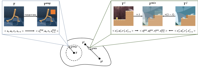
Figure 9: Contrast between augmenting observations via local perturbations (left, Cutout-Color [86]) and augmenting observations along with the supervision signals through linear interpolation (right, MixReg [49]).

An intuitive solution is to apply interpolation across different data points instead of performing a local perturbation on each individual data point. Inspired by Mixup [94] and CutMix [97], MixReg [49] convexly combines two observations and their supervision signals to generate augmented data. For example, let $y_{i}$ and $y_{j}$ denote the signals for states $s_{i}$ and $s_{j}$, respectively, which can be the reward or state values. After interpolating the observations by $\tilde{s}=\lambda s_{i}+(1-\lambda)s_{j}$, MixReg introduces mixture regularization in a similar manner via $\tilde{y}=\lambda y_{i}+(1-\lambda)y_{j}$, which helps learn more effective representations and smoother policies.

3.4 Trajectory Augmentation

Since observation or transition augmentation cannot directly enrich the trajectories encountered during training, to further improve the sample efficiency, PlayVirtual [24] augments the actions to generate synthesized trajectories under a self-supervised cycle consistency constraint.

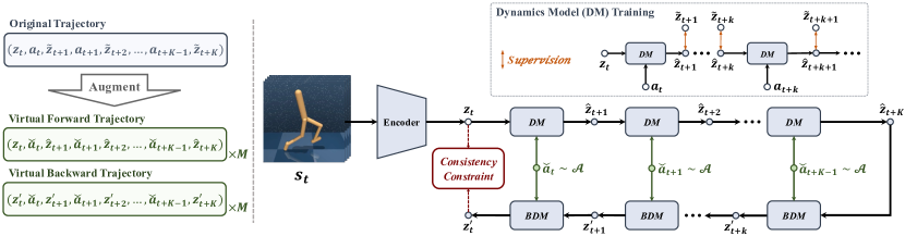
Figure 10: Data flow and architecture of PlayVirtual [24] as an example of trajectory augmentation.

In Figure 10, PlayVirtual operates entirely in the latent space after encoding the input observation $s_{t}$ into a low-dimensional state representation $z_{t}$. Following the dynamics model (DM) in SPR [23], PlayVirtual introduces a backward dynamics model (BDM) to predict the backward transition dynamics $(z_{t+1},a_{t})\longrightarrow z_{t}$ to build a loop with the forward trajectory. During the training process, the DM is supervised by the original trajectory information, whereas the BDM is constrained by the cycle consistency between $z_{t}$ and $z^{\prime}_{t}$. Further discussion on how to train the dynamics models with the auxiliary loss will be provided in Section 4.2. After obtaining the effective DM and BDM, PlayVirtual can generate diverse synthesized trajectories by randomly sampling/augmenting $M$ sets of actions in the action space $\mathcal{A}$ and then calculating the state information. Experimental studies confirmed that regularizing feature representation learning with cycle-consistent synthesized trajectories is the key to PlayVirtual’s success.

3.5 Automatic Augmentation

Automatic augmentation is receiving increasing attention due to the demand for task-specific augmentations [113, 114, 90]. For example, although random cropping is one of the most effective augmentation techniques for improving sample efficiency on many benchmarks, such as DMControl-500k [12, 13] and Procgen [54], the induced generalization ability improvement heavily depends on the specific choice of augmentation strategy. Generally, different tasks benefit from different augmentations, and selecting the most appropriate DA approach requires expert knowledge. Therefore, it is imperative to design a method that can automatically identify the most effective augmentation method. The related research in visual RL is still in its infancy [54], and we report some promising approaches below.

Upper Confidence Bound (UCB):

The task of selecting an appropriate augmentation from a given set can be formulated as a multi-armed bandit problem where the action space is the set of available transformations $F=\{f_{1},f_{2},\dots,f_{n}\}$. The UCB [115] is a popular solution for the multi-armed bandit problem that considers both exploration and exploitation. Recently, UCB-DrAC [54] and UCB-RAD [116] were proposed to achieve automatic augmentation in visual RL. The experiment results suggest that UCB-based automatic augmentations can significantly improve an agent’s generalization capabilities.

Meta Learning:

Meta learning is an alternative solution to automatic augmentation. It can be implemented in two ways [54]: $(1)$ training a meta learner such as RL² [117] to automatically select an augmentation type before every update in a DA-based algorithm; $(2)$ meta learning the weights of a CNN to perturb the observed images, which is similar to model-agnostic meta learning (MAML) [118, 119]. In practice, both approaches have not yet produced sufficiently promising results, and it remains challenging to design expressive functions for automatic augmentation based on meta learning.

3.6 Context-Aware Augmentation

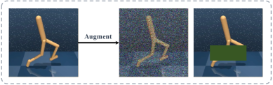
Figure 11: Context-agnostic augmentation.

Another deficiency of current DA methods is that they rely on pixel-level image transformations, where each pixel is treated in a context-agnostic manner [81]. However, in visual RL, the pixels in an observation are likely to have different levels of relevance to the decision making process [120, 121]. Figure 11 shows that the context-agnostic augmentation may mask or destroy regions in the original observation that are vital for decision making. This context-agnostic property explains why the naive application of prior-based strong augmentation may severely damage both the sample efficiency and the training stability of visual RL, regardless of its potential to enhance generalization [15, 81]. Therefore, it is necessary to incorporate context awareness into augmentation, and two viable solutions are available for doing so.

1. Introducing human guidance. Human-in-the-loop RL (HIRL) [122] is a general paradigm that leverages human guidance to assist the RL process. EXPAND [123] introduces a human saliency map to mark the importance levels of different regions, and it only perturbs the irrelevant regions. Saliency maps contain human domain knowledge, allowing context information to be embedded into the augmentation.

2. Excavating task relevance. In visual RL, the contextual information can be extracted from the task relevance of each pixel, making it possible to directly determine its task relevance to achieve context-aware augmentation. Task-aware Lipschitz DA (TLDA) [81] explicitly defines the task relevance by computing the Lipschitz constants produced when perturbing corresponding pixels. Regions with large Lipschitz constants are crucial for the current task decision, and these regions will subsequently be protected from augmentation.

Context-aware augmentation is the foundation for semantic-level DA, which is challenging and pivotal [124, 81]. In Section 6.1, we will further discuss semantic-level DA as an important direction for future studies.

4 How to Leverage Augmented Data in Visual RL?

Next, we discuss how to exploit the augmented data in visual RL. To ease the discussion, we divide the application scenarios where DA plays a vital role into three cases.

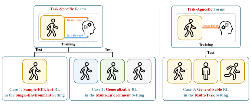
Figure 12: Three representative cases where DA plays a vital role.

1. Sample-efficient RL in the single-environment setting. Agents are trained and evaluated in the same fixed environment, and this is referred to as the single-environment setting [6]. The goal is to achieve satisfactory performance with limited environment interactions [13].

2. Generalizable RL in the multi-environment setting. Agents are tested in unseen environments after interacting with the training environments [48]. Since RL agents tend to overfit the training environment [16], generalizing the learned policies to unseen environments remains challenging even when only visual appearances are altered.

3. Generalizable RL in the multi-task setting. Agents in the multi-task setting aim to adapt to different tasks. Traditional end-to-end RL algorithms heavily rely on task-specific rewards, making them unsuitable for other tasks [38]. Recent studies have attempted to solve this issue by pretraining a cross-task representation in a task-agnostic manner so that the agent can quickly adapt to multiple downstream tasks [125].

In Figure 12, RL agents are trained with task-specific rewards in Case $1$ and Case $2$, where DA is implemented as an implicit regularization penalty when enlarging the training set (Section 4.1). However, the effect of implicit regularization is limited [23], and many studies have attempted to design auxiliary losses to exploit the potential of DA (Section 4.2). Some studies have also aimed to decouple representation learning from policy optimization to attain more generalizable policies [48] (Section 4.3). Finally, the related works belonging to Case 3, referred to as task-agnostic representation approaches using unsupervised learning, are introduced in Section 4.4.

4.1 Implicit Policy Regularization

DNNs are capable of learning complex representational spaces, which is essential for tackling intricate learning tasks. However, the model capacity required to capture such high-dimensional representations makes these techniques difficult to optimize and prone to overfitting [126]. Moreover, the complexity of visual RL is further aggravated by the need to jointly learn representations and policies directly from high-dimensional observations based on sparse reward signals [6, 12]. As a result, it is difficult for agents to distinguish the task-relevant (reward-relevant) features from high-dimensional observations, and they may mistakenly correlate rewards with spurious features [56]. To solve these issues, researchers have conducted a series of studies to develop effective regularization techniques, which can prevent overfitting and improve generalization by incorporating the inductive biases of model parameters [126].

In RL, a myriad of techniques have been proposed as regularizers such as $L^{p}$-norm regularization [4], batch normalization [76], weight decay [18] and dropout [77]. Among them, $L^{p}$-norm regularization explicitly includes regularization terms as additional constraints, and is referred to as explicit regularization [56]. Conversely, weight decay and dropout aim to tune the optimization process without affecting the loss function, making them implicit regularization strategies [77]. Additionally, DA has been prevalent in the deep learning community as a data-driven technique [51, 80]. Furthermore, increasing efforts have been devoted to the theoretical underpinnings behind DA [127, 128, 84, 83, 129] to explain its regularization effects, including the derivation of an explicit regularizer to simulate the behaviors of DA [127].

The initial and naive practice of DA is to expand the training set with augmented (synthesized) samples [130]. This practice incorporates prior-based human knowledge into the data instead of designing explicit penalty terms or modifying the optimization procedure. Hence, it is often classified as a type of implicit regularization, formulated as the empirical risk minimization on augmented data (DA-ERM) [128] in SL tasks:

$$\widehat{h}^{da-erm}\triangleq\underset{h\in\mathcal{H}}{\operatorname{argmin}}\sum_{i=1}^{N}l\left(h\left(\mathbf{x}_{i}\right),y_{i}\right)+\sum_{i=1}^{N}\sum_{j=1}^{\alpha}l\left(h\left(\mathbf{x}_{i,j}\right),y_{i}\right)$$ (10)

where $\left(\mathbf{x}_{i},y_{i}\right)$ is the $i^{\text{th}}$ original training sample ($\mathbf{x}_{i}\in\mathcal{X}$ is the input feature, and $y_{i}\in\mathcal{Y}$ is its label); $\mathbf{x}_{i,j}$ denotes the $j^{\text{th}}$ augmented sample of $\mathbf{x}_{i}$ that preserves the corresponding label $y_{i}$; $\alpha$ is the number of augmentations; $l:\mathcal{Y}\times\mathcal{Y}\rightarrow\mathbb{R}$ is the loss function and $h(\cdot)$ is the model to be optimized.

In the visual RL community, RAD [12] and DrQ [13] first leverage classical image transformation strategies such as cropping to augment the input observations via the implicit regularization paradigm. In the original paper, DrQ is proposed with two distinct ways to regularize the Q-function. On the one hand, it uses $K$ augmented observations from the original $s_{i}^{\prime}$ to obtain the target values for each transition tuple $(s_{i},a_{i},r_{i},s_{i}^{\prime})$:

$$y_{i}=r_{i}+\gamma\frac{1}{K}\sum_{k=1}^{K}Q_{\theta}(f(s_{i}^{\prime},\nu_{i,k}^{\prime}),a_{i,k}^{\prime}),a_{i,k}^{\prime}\sim\pi(\cdot\mid f(s_{i}^{\prime},\nu_{i,k}^{\prime}))$$ (11)

where $f:\mathcal{S}\times\mathcal{T}\rightarrow\mathcal{S}$ is the augmentation function and $\nu$ is the parameter of $f(\cdot)$, which is randomly sampled from the set of all possible parameters $\mathcal{T}$. Alternatively, DrQ generates $M$ different augmentations of $s_{i}$ to estimate the Q-function:

$$J_{Q}^{\mathrm{DrQ}}(\theta)=\frac{1}{NM}\sum_{i=1,m=1}^{N,M}||Q_{\theta}(f(s_{i},\nu_{i,m}),a_{i})-y_{i}||^{2}_{2}$$ (12)

In the above, DrQ leverages DA for improved estimation without adding any penalty terms, which is a type of data-driven implicit regularization. Since a sample can be defined as a tuple $(\mathbf{x}_{i},y_{i})$ in SL or a transition $(s_{i},a_{i},r_{i},s_{i}^{\prime})$ in RL, the optimization objective of DrQ can be rewritten as:

$$J_{Q}^{\mathrm{DrQ}}(\theta)=\frac{1}{NMK}\sum_{i=1}^{N}\sum_{m=1}^{M}\sum_{k=1}^{K}l(f(s_{i},\nu_{i,m}),a_{i},r_{i},f(s_{i}^{\prime},\nu_{i,k}^{\prime}))$$ (13)

where $l(s_{i},a_{i},r_{i},s_{i}^{\prime})=||Q_{\theta}(s_{i},a_{i})-(r_{i}+\gamma Q_{\theta}(s_{i}^{\prime},a_{i}^{\prime}))||^{2}_{2}$ is the loss function, and $a_{i}^{\prime}\sim\pi(\cdot\mid s_{i}^{\prime})$. RAD [12] can be regarded as a specific form of DrQ with $K=1$ and $M=1$; it is a plug-and-play module that can be plugged into any RL method (on-policy methods such as PPO [3] and off-policy methods such as SAC [17]) without making any changes to the underlying algorithm. RAD has also highlighted the generalization benefits of DA on OpenAI Procgen [131]. Since RAD and DrQ directly optimize the RL objective on multiple augmented observation views without any auxiliary losses, they can be viewed as implicit approaches for ensuring consistency and invariance among the augmented views.

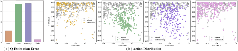
Figure 13: $Q$-estimation errors and action distributions for augmented and original data. (a) Mean absolute $Q$-estimation errors of the converged DrQ [13] agents for the same observations before and after augmentation (copied from [15]). (b) Action distributions between the augmented and original data. We use t-distributed stochastic neighbor embedding (t-SNE) to show the high-dimensional actions employed by the same converged DrQ agent.

However, later studies found that implicit regularization with cropping exhibits poor generalization performance in unseen environments [54, 15]. As discussed in Section 2.3, optimality-invariant transformations (represented by cropping) cannot provide sufficient visual diversity for reducing the generalization gap. Furthermore, although prior-based strong augmentations such as color jitter have the potential to improve generalization, they may induce large $Q$-estimation errors and action distribution shifts, as shown in Figure 13 [15, 81]. Hence, implicit regularization approaches with prior-based strong augmentations (e.g., random convolution and overlay) may make the RL optimization process fragile and unstable [15]. This poses a dilemma in visual RL: diverse augmentation is necessary to improve an agent’s generalization ability, but excessive data variations may damage the stability of RL [48].

SVEA [15] aims to enhance the stability of RL optimization with DA [13]. It consists of two main components. First, SVEA uses only original data copies to estimate $Q$-targets to avoid erroneous bootstrapping caused by DA, where $y_{i}=r_{i}+\gamma Q_{\theta}(s_{i}^{\prime},a_{i}^{\prime})$, $a_{i}^{\prime}\sim\pi(\cdot\mid s_{i}^{\prime})$. Second, SVEA formulates a modified $Q$-objective to estimate the $Q$-value over both augmented and original copies of the observations, which can be expressed in a modified ERM form as follows:

$$J_{Q}^{\mathrm{SVEA}}(\theta) =\alpha\sum_{i=1}^{N}||Q_{\theta}(s_{i},a_{i})-y_{i}||^{2}_{2}+\beta\sum_{i=1}^{N}\sum_{m=1}^{M}||Q_{\theta}(f(s_{i},\nu_{i,m}),a_{i})-y_{i}||^{2}_{2}$$ (14)

$$=\alpha\sum_{i=1}^{N}l(s_{i},a_{i},r_{i},s_{i}^{\prime})+\beta\sum_{i=1}^{N}\sum_{m=1}^{M}l(f(s_{i},\nu_{i,m}),a_{i},r_{i},s_{i}^{\prime})$$

Experimental studies have shown that SVEA can yield significantly improved stability under strong augmentation and achieve competitive generalization performance on the DeepMind control suite [10, 53]. Additionally, other approaches have also been explored to address this dilemma, including designing auxiliary tasks (Section 4.2) and decoupling representation learning and policy optimization (Section 4.3).

4.2 Explicit Policy Regularization with Auxiliary Tasks

Visual RL relies on the state representation, but it remains challenging to directly infer the ideal representation from high-dimensional observations [132]. A typical workflow involves designing auxiliary objectives to facilitate the representation learning process [133], or improve sample efficiency [26] or prevent observational overfitting [56]. In general, an auxiliary task can be considered as an additional cost function that the RL agent can predict and observe from the environment in a self-supervised fashion [134]. For example, the last layer of the network can be split into multiple parts (heads), each working on a specific task [34, 135]. The multiple heads then propagate errors back to the shared network layers that form the complete representations required by all heads.

With the recent success in unsupervised learning, various auxiliary tasks have been designed to produce effective representations [134, 136]. Thus, it is natural to design additional losses to explicitly constrain an agent’s policy and value functions, which we will discuss in Section 4.2.1. Moreover, we introduce contrastive learning as a lower bound of mutual information in Section 4.2.2 and future prediction objectives with a DM in Section 4.2.3.

4.2.1 DA Consistency

In contrast to simply inserting augmented data into the training dataset, DA consistency (DAC) [128] builds a regularization term to penalize the representation difference between the original sample $\phi_{h}\left(\mathbf{x}_{i}\right)$ and augmented sample $\phi_{h}\left(\mathbf{x}_{i,j}\right)$, under the assumption that similar samples should be close in the representation space:

$$\underset{h\in\mathcal{H}}{\operatorname{argmin}}\sum_{i=1}^{N}l\left(h\left(\mathbf{x}_{i}\right),y_{i}\right)+\underbrace{\lambda\sum_{i=1}^{N}\sum_{j=1}^{\alpha}\varrho\left(\phi_{h}\left(\mathbf{x}_{i}\right),\phi_{h}\left(\mathbf{x}_{i,j}\right)\right)}_{\text{DAC regularization }}$$ (15)

where $\phi_{h}$ refers to the features extracted from the high-dimensional data, which can be viewed as the output of any layer in the DNN, and $\varrho$ is the metric function defined in the representation space, which can be the $\mathcal{L}_{p}$ norm or KL divergence. As an unsupervised representation module, DAC regularization can be employed as an auxiliary task in any SL or RL algorithms to enforce the model to produce similar predictions on the original and augmented samples. For example, SODA [53] calculates the consistency loss by minimizing the $L^{2}$ norm between the features of the augmented and original observations in the latent space; SIM [137] produces a cross-correlation matrix between two embedding vector sets of the original and augmented observations, and designs an invariance loss term to ensure the invariance of data.

For RL tasks, it is also desirable to train the network to output the same policies and values for both original and augmented observations [13]. For example, DrAC [54] employs two extra loss terms: $G_{\pi}$ for regularizing the policy by the KL divergence measure and $G_{V}$ for regularizing the value function using the mean-squared deviation:

$$G_{\pi}=KL\left[\pi_{\theta}(a\mid s)\mid\pi_{\theta}(a\mid f(s,\nu))\right],\qquad G_{V}=\left(V_{\phi}(s)-V_{\phi}(f(s,\nu))\right)^{2}$$ (16)

The complete optimization objective of DrAC based on PPO is as follows:

$$J_{\mathrm{DrAC}}=J_{\mathrm{PPO}}-\alpha_{r}\left(G_{\pi}+G_{V}\right)$$ (17)

where $\alpha_{r}$ is the weight of the regularization term, and both $G_{\pi}$ and $G_{V}$ can be added to the objective of any actor-critic algorithm. By enforcing the DA consistency into the networks, specific transformations can be used to impose inductive biases relevant to the given task (e.g., invariance with respect to colors or translations) [54, 128].

Compared with implicit regularization techniques such as RAD and DrQ, DrAC employs two auxiliary consistency loss terms for explicitly regularizing the policy and the value function to ensure invariance. Instead of directly optimizing the RL objective on multiple augmented views of the observations, DAC regularization uses only the transformed observations $f(s,\nu)$ to compute the regularization losses $G_{\pi}$ and $G_{V}$. Hence, DrAC can benefit from the regularizing effect of DA while mitigating the adverse effect on the RL objective [54].

4.2.2 Contrastive Learning

Another type of auxiliary task closely related to DA is contrastive learning. As mutual information (MI) is often hard to estimate, it is practical to maximize the lower bound of MI through approaches using, for example, InfoNCE loss [73]) to train robust feature extractors [138]. Recent studies [26, 38] have shown that contrastive learning can significantly improve the sample efficiency and generalization performance of visual RL [34]. Since contrastive learning only requires unlabeled data, it can not only be performed as auxiliary tasks together with RL objectives but also be leveraged to learn a task-agnostic representation, which we will discuss in Section 4.4.

In visual RL, there are two types of contrastive learning for improving agents’ sample efficiency and generalization abilities [34]. The first class [26, 29, 28] focuses on maximizing the MI between different augmented versions of the same observation while minimizing the similarity between different observations. It tends to further exploit the regularization ability of DA at the MI level [34]. However, simply maximizing the lower bound of MI may retain the task-irrelevant information [139], which needs to be eliminated based on the information bottleneck principle. The second class [73, 38] aims to maximize the predictive MI between consecutive states by applying contrastive losses between an observation $o_{t}$ and the near-future observations $o_{t+k}$ over multiple time steps. This technique encourages the encoder to extract the temporal correlations of the latent dynamics from the observations [38], and DA can be applied as the prior-based data preprocessing.

Maximizing Multi-view MI:

In self-supervised representation learning, feature extractors can be trained by maximizing the MI between different augmented views of the original data [138], and this approach has also been extended to the domain of visual RL [26, 27].

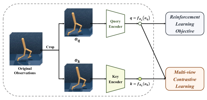
Figure 14: The workflow of contrastive unsupervised representations for RL (CURL).

CURL[26] is the first general framework for combining multi-view contrastive learning and DA in visual RL. It builds an auxiliary contrastive task to learn useful state representations by maximizing the MI between the different augmented views of the same observations to improve the transformation invariance of the learned embedding. In Figure 14, the contrastive representation is jointly trained with the RL objective, and the latent encoder receives gradients from both the contrastive learning objective and the RL objective.

A key component of contrastive learning is the selection of positive and negative samples relative to an anchor, and CURL uses instance discrimination rather than patch discrimination [26]. Specifically, the anchor and positive observations are two different augmentations of the same observation, while the negative samples come from other observations in the minibatch. The contrastive learning task in CURL aims to maximize the MI between the anchor and the positives while minimizing the MI between the anchor and the negatives.

Following the setting of momentum contrast (MoCo) [140], CURL applies DA twice to generate queries and key observations, which are then encoded by the query encoder and key encoder, respectively. The query observations $o_{q}$ are treated as the anchor, while the key observations $o_{k}$ contain the positives and negatives. During the gradient update step, only the query encoder is updated, while the key encoder weights are set to the exponential moving average (EMA) of the query weights [140]. CURL employs the bilinear inner product $\operatorname{sim}(q,k)=q^{T}Wk$ to measure the agreement between query-key pairs, where $W$ is a learned parameter matrix. Then, it uses the InfoNCE loss [73] to build an auxiliary loss function as follows:

$$\mathcal{L}_{\mathrm{InfoNCE}}=\log\frac{\exp(q^{T}Wk_{+})}{\exp(q^{T}Wk_{+})+\sum_{i=0}^{K-1}\exp(q^{T}Wk_{i})}$$ (18)

where $\{k_{0},k_{0},\dots,k_{K-1}\}$ are the keys of the dictionary and $k_{+}$ denotes a positive key. The InfoNCE loss can be interpreted as the log-loss of a $K$-way softmax classifier whose label is $k_{+}$ [138].

Many subsequently developed contrastive multi-view coding methods also employ the InfoNCE bound to maximize the MI between two embeddings that result from different augmentations. For example, DRIBO [29] aims to maximize the InfoNCE loss $\hat{I}_{\psi}({o}_{t}^{(1)},{o}_{t}^{(2)})$, where $\psi$ represents the learnable parameters. Furthermore, ADAT [28] selects the positive observations with the same action type and the negatives with other actions so that more positives can be produced. CCLF [27] introduces a curiosity appraisal module to select the most informative augmented observations for enhancing the effect of multi-view contrastive learning.

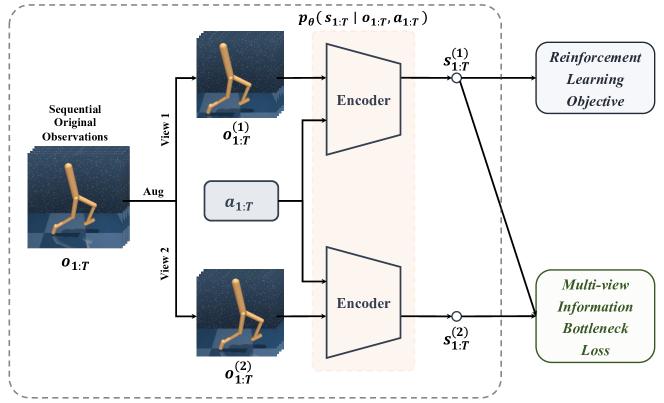
Figure 15: The workflow of deep RL via multi-view infomration bottleneck (DRIBO).

Although maximizing the similarity between augmented versions of the same observation is valuable for state representation [26, 34], maximizing the lower-bound of MI may inevitably retain some task-irrelevant information, limiting the generalization abilities of agents. To tackle this issue, DRIBO [29] uses contrastive learning combined with a multi-view information bottleneck (MIB)-based auxiliary objective to learn representations that contain only task-relevant information that is predictive of the future while eliminating task-irrelevant information.

The assumption of DRIBO is that a desired representation for RL should facilitate the prediction of future states and discard excessive, task-irrelevant information from visual observations. In Figure 15, the augmented observations share the same task-relevant information, while any information not shared by them is regarded as being task-irrelevant [29]. In practice, the task-relevant MI can be maximized by InfoNCE, as in CURL. With the information bottleneck principle, DRIBO constructs a relaxed Lagrangian loss to obtain a sufficient representation with minimal task-irrelevant information, and the task-irrelevant minimization term is upper-bounded by:

$$\mathcal{L}_{\mathrm{SKL}}=D_{\mathrm{SKL}}(p_{\theta}(\bm{s}_{t}^{(1)}\mid\bm{o}_{t}^{(1)},\bm{s}_{t-1}^{(1)},\bm{a}_{t-1})\mid\mid p_{\theta}(\bm{s}_{t}^{(2)}\mid\bm{o}_{t}^{(2)},\bm{s}_{t-1}^{(2)},\bm{a}_{t-1}))$$ (19)

where $D_{\mathrm{SKL}}$ represents the symmetrized KL divergence based on the probability densities of $\bm{s}_{t}^{(1)}$ and $\bm{s}_{t}^{(2)}$ obtained using the encoder. Experiments have shown that DRIBO yields significantly improved generalization and robustness on the DeepMind control suite [10] and Procgen [131] benchmarks.

Maximizing Temporal Predictive MI:

Another popular strategy for representation learning is to learn a compact predictive coding to predict future states or information, which can also be combined with DA. The first approach is to directly minimize the prediction error between the true future states and the predicted future states via a dynamic transition model, which will be discussed in Section 4.2.3. Another approach is to maximize the lower bound of the MI between the embeddings of consecutive time steps to induce predictive representations without relying on a generative model.

CPC [73] and ST-DIM [30] use temporal contrastive losses to maximize the MI between the previous state embedding and a future embedding several time steps later, but they both do not leverage DA to transform the observations. Recently, ATC [38], CCFDM [31] and CoDy [34] apply DA to regularize the observations obtained prior to encoding, imposing an inductive bias on information not relevant to the agent. For example, $\mathcal{L}_{\mathrm{TMI}}$ in CoDy [34] aims to maximize the InfoNCE bound on the temporal MI between the embedding of the current state and action and the true embedding of the next state to increase the linearity of the latent dynamics. In practice, this approach first randomly draws a minibatch of transitions $(s_{t},a_{t},s_{t+1})$ from the replay buffer. Then, it obtains a minibatch of positive sample pairs $(z_{t}^{1},c_{t},z_{t+1})$ by feeding $s_{t},a_{t}$ and $s_{t+1}$ into their corresponding encoders. For a given positive sample pair $(z_{t}^{1},c_{t},z_{t+1})$, it constructs negative samples by replacing $z_{t+1}$ with all features $z_{t+1}^{*}$ from other sample pairs $(z_{t}^{1^{*}},c_{t}^{*},z_{t+1}^{*})$ in the same minibatch. Furthermore, M-CURL [32] leverages a bidirectional transformer to reconstruct the features of the masked observations from their surrounding observations. It then captures the temporal dependency by minimizing the contrastive loss between the reconstructed and original features.

4.2.3 Future Prediction with a DM

The motivation of future prediction tasks is to encourage state representations to be predictive of future states given the current state and future action sequence [34]. Instead of maximizing the MI between the current state and the future state using the InfoNCE loss [73, 30, 38], SPR [23] produces state representations by minimizing the prediction error between the true future states and the predicted future states using an explicit multi-step DM. As shown in Figure 16, this approach also incorporates DA into the future prediction task, which enforces consistency across different views of each observation.

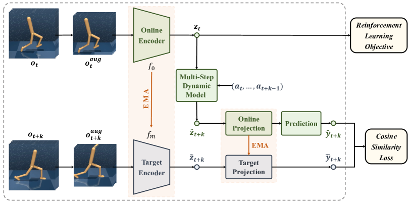
Figure 16: The workflow of self-predictive representations (SPR).

The DM $h(\cdot,\cdot)$ operates entirely in the latent space to predict the transition dynamics $\left(\mathbf{z}_{t},a_{t}\right)\rightarrow\mathbf{z}_{t+1}$, where $\mathbf{z}_{t}=f\left(\mathbf{o}_{t}\right)$ is encoded by the feature encoder $f(\cdot)$ of the current input observation $o_{t}$. The prediction loss is computed by summing up the differences (errors) between the predicted representations $\hat{\mathbf{z}}_{t+1:t+K}$ and the observed representations $\tilde{\mathbf{z}}_{t+1:t+K}$:

$$\mathcal{L}_{\mathrm{pred}}=\sum_{k=1}^{K}d\left(\hat{\mathbf{z}}_{t+k},\tilde{\mathbf{z}}_{t+k}\right)=-\sum_{k=1}^{K}\left(\frac{\tilde{\mathbf{z}}_{t+k}}{\left\|\tilde{\mathbf{z}}_{t+k}\right\|_{2}}\right)^{\top}\left(\frac{\hat{\mathbf{z}}_{t+k}}{\left\|\hat{\mathbf{z}}_{t+k}\right\|_{2}}\right)$$ (20)

where the latent representation $\hat{\mathbf{z}}_{t+1:t+K}$ is computed iteratively as $\hat{\mathbf{z}}_{t+k+1}\triangleq h\left(\hat{\mathbf{z}}_{t+k},a_{t+k}\right)$, starting from $\hat{\mathbf{z}}_{t}\triangleq\mathbf{z}_{t}\triangleq f_{o}\left(o_{t}\right)$, and $\tilde{\mathbf{z}}_{t+k}\triangleq f_{m}\left(o_{t+k}\right)$ is computed by the target encoder $f_{m}$, whose parameters are the EMAs of the parameters of the online encoder $f_{o}$. Combined with DA, SPR improves the agent’s sample efficiency and results in superior performance with limited iterations on Atari Games and the DeepMind control suite [23].

PlayVirtual [24] is an extension of SPR that introduces cycle consistency to generate augmented virtual trajectories for achieving enhanced data efficiency. Following the DM in SPR [23], PlayVirtual [24] proposes a BDM for backward state prediction to build a cycle/loop with a forward trajectory. Given a DM $h(\cdot,\cdot)$, a BDM $b(\cdot,\cdot)$, the current state representation $\mathbf{z}_{t}$, and a sequence of actions $a_{t:t+K}$, a forward trajectory and the corresponding backward trajectory can be generated to form a synthesized trajectory:

Forward $$:\hat{\mathbf{z}}_{t}=\mathbf{z}_{t},\hat{\mathbf{z}}_{t+k+1}=h\left(\hat{\mathbf{z}}_{t+k},\mathbf{a}_{t+k}\right),\text{ for }k=0,1,\cdots,K-1$$ (21)

Backward $$:\mathbf{z}_{t+K}^{\prime}=\hat{\mathbf{z}}_{t+K},\mathbf{z}_{t+k}^{\prime}=b\left(\mathbf{z}_{t+k+1}^{\prime},\mathbf{a}_{t+k}\right),\text{ for }k=K-1,K-2,\cdots,0$$

Since cycle consistency can be enforced by constraining the distance between the starting state $\mathbf{z}_{t}$ and the ending state $\mathbf{z}_{t}^{\prime}$ in the loop, appropriate synthesized training trajectories can be obtained by augmenting actions. In practice, the cycle consistency loss can be calculated by randomly sampling $M$ sets of actions from the action space $\mathcal{A}$:

$$\mathcal{L}_{\mathrm{cyc}}=\frac{1}{M}\sum_{m=1}^{M}d_{\mathcal{M}}\left(\mathbf{z}_{t}^{\prime},\mathbf{z}_{t}\right)$$ (22)

where $d_{\mathcal{M}}$ is the distance metric over the latent space $\mathcal{M}$. The performance of PlayVirtual [24] can be explained from two aspects. First, the generated trajectories can help the agent "see" more flexible experiences. Second, enforcing the trajectory with the cycle consistency constraint can further regularize the feature representation learning process.

4.3 Task-Specific Representation Decoupled from Policy Optimization

Utilizing DA as an implicit [12, 13, 105] or explicit regularization approach with purposefully designed auxiliary tasks [26, 23, 34], the sample efficiency of visual RL has been significantly improved, resulting in performance comparable to state-based algorithms on several benchmarks [14]. However, training generalizable RL agents that are robust against irrelevant environmental variations remains a challenging task. Similar challenges in SL tasks, such as image classification, can be addressed by strong augmentations that heavily distort the input images, such as Mixup [94] and CutMix [97]. However, since the training process of RL is vulnerable to excessive data variations, a naive application of DA may severely damage the training stability [15, 48].

This poses a dilemma: aggressive augmentations are necessary for achieving good generalization in the visual domain [141], but injecting heavy DA into the optimization of an RL objective may cause deterioration in both the sample efficiency and the training stability [81]. Recent works [53, 48] argued that this is mainly due to the conflation of two objectives: policy optimization and representation learning. Hence, an intuitive idea is to decouple the training data flow by using nonaugmented or weakly augmented data for RL optimization while using strongly augmented data for representation learning. As shown in Figure 17, two strategies are available for achieving the decoupling goal: $(1)$ dividing the training data into two streams to separately optimize $\mathcal{L}_{RL}$ and $\mathcal{L}_{SSL}$; and iteratively updating the model parameters by the two objectives [53]; $(2)$ optimizing the RL objective $\mathcal{L}_{RL}$ first and then sequentially leveraging DA combined with SSL objective $\mathcal{L}_{SSL}$ for knowledge distillation [48].

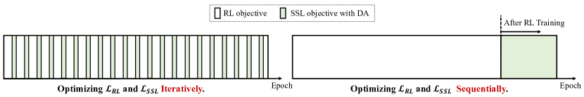
Figure 17: Different strategies for decoupling policy optimization and representation learning.

Optimizing $\mathcal{L}_{RL}$ and $\mathcal{L}_{SSL}$ Iteratively:

This strategy aims to divide the training data into two data streams and only uses the nonaugmented or weakly augmented data for the RL training process; it leverages strong augmentations under prior-based diversity assumptions to optimize the self-supervised representation objective and enhance the generalization ability of the model. In practice, this technique can be performed by iteratively optimizing the RL objective $\mathcal{L}_{RL}$ and the self-supervised representation objective $\mathcal{L}_{SSL}$ in combination with DA to update the network parameters. For example, SODA [53] maximizes the MI between the latent representations of augmented and nonaugmented data as the auxiliary objective $\mathcal{L}_{\mathrm{SODA}}$, and continuously alternates between optimizing $\mathcal{L}_{RL}$ with nonaugmented data and $\mathcal{L}_{\mathrm{SODA}}$ with augmented data. While a policy is learned only from nonaugmented data, SODA still substantially benefits from DA through representation learning [53].

Optimizing $\mathcal{L}_{RL}$ and $\mathcal{L}_{SSL}$ Sequentially:

This is a two-stage training strategy, which first trains a sample-efficient agent using weak augmentations, and then enhances the state representation by auxiliary self-supervised learning or imitation learning with strong augmentations. For example, SECANT [48] first trains a sample-efficient expert with random cropping (weak augmentation). In the second stage, a student network learns a generalizable policy by mimicking the behavior of the expert at every time step but with a crucial difference: the expert produces the ground-truth actions from unmodified observations, while the student learns to predict the same actions from heavily corrupted observations, as shown in Figure 18. The student optimizes the imitation objective by performing gradient descent on a supervised regression loss: $\mathcal{L}\left(o;\theta_{s}\right)=\left\|\pi_{s}(f(o))-\pi_{e}(o)\right\|_{F}$, which has better training stability than the RL loss. Furthermore, conducting policy distillation through strong augmentations can greatly remedy overfitting so that robust representations can be acquired without sacrificing policy performance.

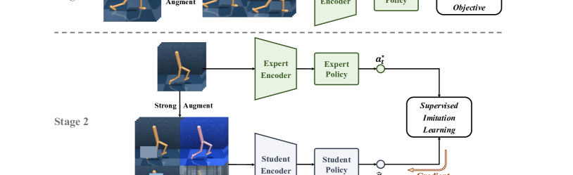
Figure 18: The workflow of self expert cloning for adaptation to novel test-env (SECANT).

4.4 Task-Agnostic Representation Using Unsupervised Learning

Unsupervised/self-supervised pretraining, a framework that trains models without supervision, has achieved remarkable success in various domains [142, 143, 144] and can efficiently solve downstream tasks through fine-tuning. Similarly, it is also reasonable to learn an unsupervised pretrained RL agent that can quickly adapt to diverse test tasks in a zero-shot or few-shot manner [40, 43]. Furthermore, some recent studies [38] argued that the visual representations of standard end-to-end RL methods heavily rely on task-specific rewards, making them ineffective for other tasks. To overcome this limitation, the environment can be first explored in a task-agnostic fashion to learn its visual representations without any task-specific rewards, and specific downstream tasks can subsequently be efficiently solved [38, 39]. Another key application of task-agnostic representation considers multi-task settings where, with the same or similar visual scenes, different downstream tasks are defined by corresponding reward functions. For instance, the Walker domain in the DeepMind control suite [10] consists of multiple tasks, including standing, walking forward, flipping backward, etc.

Two strategies are available for learning an encoder that maps a high-dimensional input to a compact representation in a task-agnostic fashion. The first approach is to design unsupervised representation tasks, as in Section 4.2. Second, we can maximize the intrinsic rewards to encourage meaningful behaviors in the absence of external rewards, which are derived from self-supervised forms such as the particle-based entropy and curiosity [145, 40, 39, 146, 147]. With the ability of DA to promote prior discrimination, many unsupervised pretraining studies combine DA with other auxiliary tasks to learn more meaningful representations. For example, ATC [38] applies random cropping combined with contrastive learning as the task-agnostic representation tasks, while APT [40] and SGI [147] leverage DA to design self-predictive tasks.

5 Experimental Evaluation

This section provides a systematic empirical evaluation of the methods in visual RL that leverage DA. First in Section 5.1, we introduce the commonly used benchmarks for evaluating the sample efficiency and generalization ability of agents. Then in Section 5.2 and Section 5.3, we present the experimental results of representative RL techniques using DA in comparison with those of other baselines to demonstrate the effectiveness of DA and identify the pros and cons of these methods.

5.1 Representative Benchmarks

5.1.1 Benchmarks for Sample Efficiency Evaluating in Visual RL

Atari Games [148]

This suite of games is widely used by both state-based and image-based discrete control algorithms for sample-constrained evaluations [2]. While RL algorithms can achieve superhuman performance on Atari games, they are still far less efficient than human learners, especially in image-based cases [26]. In the sample-efficient Atari-100k setting, only 100k interactions (400k frames with frame-skip=4) are available. The performance of an agent on a game is measured by its human-normalized score (HNS), defined as $\frac{S_{A}-S_{R}}{S_{H}-S_{R}}$ where $S_{A}$ is the agent’s score; $S_{R}$ is the score of a random play; $S_{H}$ is the expert human score.

DeepMind Control Suite [10]

This is a continuous control benchmark suite for evaluating visual RL algorithms. It presents a variety of challenging tasks, including bipedal balancing, locomotion, contact forces, and goal reaching, with both sparse and dense reward signals. Previous studies usually measured the data efficiency and performance of their algorithms on the DeepMind control suites with 100k (for measuring learning speed) and 500k (for measuring overall performance) environment steps, which are referred to as DMControl-100k and DMControl-500k, respectively. DeepMind control suite is also a proper testbed for multi-task settings, as different tasks often involve the same domain. For example, the walker domain contains running, walking, standing and many other tasks, allowing agents to transfer learned policies to other tasks with similar visual observations.

5.1.2 Benchmarks for Generalization Evaluating in Visual RL

Although Atari Games and the DeepMind control suite are suitable for benchmarking the sample efficiency of visual RL agents, they are not applicable for investigating the generalization abilities of these agents [12]. Generally, measuring the generalization ability of an agent requires variations between the training environment and the test environment, including state-space variations (the initial state distribution), dynamics variations (the transition function), visual variations (the observation function), and reward function variations [55]. In particular, DA-based techniques focus on zero-shot generalization to unseen environments with similar high-level goals and dynamics but different layouts and visual properties [15, 105, 149]. Figure 19 shows the representative benchmarks for evaluating the agent’s generalization ability in visual RL.

Figure 19: Typical benchmarks used to evaluate an agent’s generalization ability in visual RL.

OpenAI Procgen [131]

This is a suite of game-like environments where different levels feature varying visual attributes. Different combinations of the game levels can be used to separately construct training and test environments. Agents are only allowed to be trained on limited levels and are evaluated on unseen levels with different backgrounds or layouts [49, 105].

DeepMind Lab [150]

This is a first-person 3D maze environment in which various objects are placed in the rooms. As a measure of their generalization ability, agents are trained to collect objects in a fixed map layout and tested in unseen environments that differ only in terms of their walls and floors (i.e., the variational contexts) [91].

DeepMind Control Suite Variants [151, 53, 55]

Since the original DeepMind control suite is not applicable for studying generalization, a number of variants have been proposed in recent years. Most of them, such as DMControl-GB [53], DMControl-Remastered [152] and Natural Environments [153], focus on visual generalization by changing the colors or styles of the background and floors. Furthermore, the Distracting Control Suite (DCS) [151] features a broader set of variations, including background style and camera pose variations.

CARLA [66]

This is a realistic driving simulator where the agent’s goal is to drive as far as possible in 1000 time steps without colliding into 20 other moving vehicles or barriers [48]. Learning directly from the rich observations in this scenario is challenging since diverse types of task-irrelevant distractors (e.g., lighting conditions, shadows, realistic rain, clouds, etc.) are available around the agent, which increases the difficulty of extracting control-related features.

5.2 Sample Efficiency Evaluation

To measure the sample efficiency, we report the results on three common benchmarks: Atari-100k [148], DMControl-100k and DMControl-500k [10].

5.2.1 Atari-100k

In Table 1, the results of a random player (Random) and an expert human player (Human) are copied from [154] as baselines. Other scores are copied from their original papers [13, 27, 28, 32, 23, 24]. The results show that augmenting the observations as implicit regularization is effective, boosting the performance in terms of the median HNS from $5.8\%$ (Efficient DQN) to $26.8\%$ (DrQ). Moreover, appropriate auxiliary tasks such as contrastive learning [26, 32, 27, 28] and future prediction representation [23, 155, 24] can further yield improved sample efficiency. Among them, SPR [23] achieves the highest mean HNS value ($70.4\%$) with its future prediction module, while PlayVirtual [24] achieves the highest median HNS value ($47.2\%$) with the trajectory augmentation.

Table 1: Evaluation of Sample Efficiency on Atari-100k. We report the scores and the mean and median HNSs achieved by different methods on Atari-100k. The results are copied from the original works [13, 27, 28, 32, 23, 24].

Game	Human	Random	DQN	CURL	CCLF	ADAT	DrQ	M-CURL	SPR	PlayVirtual
			[2]	[26]	[27]	[28]	[13]	[32]	[23]	[24]
Alien	$7127.7$	$227.8$	$558.1$	$558.2$	$920.0$	$1029.7$	$771.2$	${\color[rgb]{0.75390625,0,0}\bm{1151.6}}$	$801.5$	$947.8$
Amidar	$1719.5$	$5.8$	$63.7$	$142.1$	$154.7$	$147.3$	$102.8$	${\color[rgb]{0.75390625,0,0}\bm{182.2}}$	$176.3$	$165.3$
Assault	$742.0$	$222.4$	$589.5$	$600.6$	$612.4$	${\color[rgb]{0.75390625,0,0}\bm{749.4}}$	$452.4$	$613.5$	$571.0$	$702.3$
Asterix	$8503.3$	$210.0$	$341.9$	$734.5$	$708.8$	$864$	$603.5$	$738.1$	${\color[rgb]{0.75390625,0,0}\bm{977.8}}$	$933.3$
Bank Heist	$753.1$	$14.2$	$74.0$	$131.6$	$36.0$	$164$	$168.9$	$220$	${\color[rgb]{0.75390625,0,0}\bm{380.9}}$	$245.9$
Battle Zone	$37187.5$	$2360.0$	$4760.8$	$14870.0$	$5775.0$	$21240$	$12954.0$	${\color[rgb]{0.75390625,0,0}\bm{21600}}$	$16651.0$	$13260.0$
Boxing	$12.1$	$0.1$	$-1.8$	$1.2$	$7.4$	$0.4$	$6.0$	$5.9$	$35.8$	${\color[rgb]{0.75390625,0,0}\bm{38.3}}$
Breakout	$30.5$	$1.7$	$7.3$	$4.9$	$2.7$	$4.5$	$16.1$	$5.7$	$17.1$	${\color[rgb]{0.75390625,0,0}\bm{20.6}}$
Chopper Command	$7387.8$	$811.0$	$624.4$	$1058.5$	$765.0$	$1106$	$780.3$	${\color[rgb]{0.75390625,0,0}\bm{1138.9}}$	$974.8$	$922.4$
Crazy Climber	$35829.4$	$10780.5$	$5430.6$	$12146.5$	$7845.0$	$21240$	$20516.5$	$20781.2$	${\color[rgb]{0.75390625,0,0}\bm{42923.6}}$	$23176.7$
Demon Attack	$1971.0$	$152.1$	$403.5$	$817.6$	${\color[rgb]{0.75390625,0,0}\bm{1360.9}}$	$851.9$	$1113.4$	$864.4$	$545.2$	$1131.7$
Freeway	$29.6$	$0.0$	$3.7$	$26.7$	$22.6$	${\color[rgb]{0.75390625,0,0}\bm{29.7}}$	$9.8$	$28.9$	$24.4$	$16.1$
Frostbite	$4334.7$	$65.2$	$202.9$	$1181.3$	$1401.0$	$1943.2$	$331.1$	${\color[rgb]{0.75390625,0,0}\bm{2342.2}}$	$1821.5$	$1984.7$
Gopher	$2412.5$	$257.6$	$320.8$	$669.3$	${\color[rgb]{0.75390625,0,0}\bm{814.7}}$	$601.2$	$636.3$	$453.8$	$715.2$	$684.3$
Hero	$30826.4$	$1027.0$	$2200.1$	$6279.3$	$6944.5$	$7259.2$	$3736.3$	$7360.6$	$7019.2$	${\color[rgb]{0.75390625,0,0}\bm{8597.5}}$
Jamesbond	$302.8$	$29.0$	$133.2$	$471.0$	$308.8$	${\color[rgb]{0.75390625,0,0}\bm{635.7}}$	$236.0$	$436.2$	$365.4$	$394.7$
Kangaroo	$3035.0$	$52.0$	$448.6$	$872.5$	$650.0$	$956.9$	$940.6$	$1691.4$	${\color[rgb]{0.75390625,0,0}\bm{3276.4}}$	$2384.7$
Krull	$2665.5$	$1598.0$	$2999.0$	${\color[rgb]{0.75390625,0,0}\bm{4229.6}}$	$3975.0$	$3502.9$	$4018.1$	$3240.9$	$3688.9$	$3880.7$
Kung Fu Master	$22736.3$	$258.5$	$2020.9$	$14307.8$	$12605.0$	${\color[rgb]{0.75390625,0,0}\bm{19146}}$	$9111.0$	$17645.6$	$13192.7$	$14259.0$
Ms Pacman	$6951.6$	$307.3$	$872.0$	$1465.5$	$1397.5$	$1075$	$960.5$	${\color[rgb]{0.75390625,0,0}\bm{1758.9}}$	$1313.2$	$1335.4$
Pong	$14.6$	$-20.7$	$-19.4$	$-16.5$	$-17.3$	$-15.1$	$-8.5$	$-8.9$	$-5.9$	${\color[rgb]{0.75390625,0,0}\bm{-3.0}}$
Private Eye	$69571.3$	$24.9$	$351.3$	$218.4$	$100.0$	${\color[rgb]{0.75390625,0,0}\bm{388}}$	$-13.6$	$321.6$	$124.0$	$93.9$
Qbert	$13455.0$	$163.9$	$627.5$	$1042.4$	$953.8$	$1578$	$854.4$	$1785$	$669.1$	${\color[rgb]{0.75390625,0,0}\bm{3620.1}}$
Road Runner	$7845.0$	$11.5$	$1491.9$	$5661.0$	$11730.0$	$12508$	$8895.1$	$12320$	${\color[rgb]{0.75390625,0,0}\bm{14220.5}}$	$13534.0$
Seaquest	$42054.7$	$68.4$	$240.1$	$384.5$	$550.5$	$251.6$	$301.2$	$481.1$	${\color[rgb]{0.75390625,0,0}\bm{583.1}}$	$527.7$
Up N Down	$11693.2$	$533.4$	$2901.7$	$2955.2$	$3376.3$	$3597.8$	$3180.8$	$4399.5$	${\color[rgb]{0.75390625,0,0}\bm{28138.5}}$	$10225.2$
Mean HNS ($\%$)	$100$	$0$	$13.7$	$38.1$	$38.2$	$47.2$	$35.7$	$46.6$	${\color[rgb]{0.75390625,0,0}\bm{70.4}}$	$63.7$
Median HNS ($\%$)	$100$	$0$	$5.8$	$17.5$	$18.1$	$20.6$	$26.8$	$34.0$	$41.5$	${\color[rgb]{0.75390625,0,0}\bm{47.2}}$
# Superhuman	N/A	0	$1$	$2$	$3$	$6$	$2$	$3$	${\color[rgb]{0.75390625,0,0}\bm{7}}$	$4$
# SOTA	N/A	0	$0$	$1$	$2$	$5$	$0$	$6$	${\color[rgb]{0.75390625,0,0}\bm{7}}$	$5$

5.2.2 DMControl-100k and DMControl-500k

Compared with Atari games, the tasks in the DeepMind control suite [10] are more complex and challenging. We first report the performance of the underlying SAC algorithm [17] based on state and image inputs, referred to as Pixel SAC and State SAC in Table 2 (copied from [26]), respectively, followed by the results of SAC-AE [6]. Since State SAC operates on low-dimensional state-based features instead of pixels, it approximates the upper bounds of sample efficiency in these environments for image-based agents. Similar to the case of Atari-100k, DrQ [13] achieves significant improvements over the underlying SAC algorithm [17], which is unable to complete these tasks. Combining auxiliary tasks with DA provides improved performance and potential for training sample-efficient agents. For example, based on SPR [23], recent studies have achieved superior performance by introducing cycle consistency constraints for more diverse trajectories (PlayVirtual [24]) or curiosity modules for better exploration (CCFDM [31]).

Table 2: Evaluation of Sample Efficiency on the DeepMind Control Suite. The reported scores (means and standard deviations) are achieved by different methods on DMControl-100k and DMControl-500k. The results are copied from their original works with 10 random seeds [6, 26, 13, 23, 24, 27, 31, 34].

DMControl	Pixel	SAC-AE	CURL	DrQ	SPR	CCLF	CoDy	MLR	CCFDM	PlayVirtual	State
100k	SAC	[6]	[26]	[13]	[23]	[27]	[34]	[21]	[31]	[24]	SAC
Finger,	$179$	$747$	$767$	$901$	$868$	${\color[rgb]{0.75390625,0,0}\bm{944}}$	$887$	$907$	$880$	$915$	$811$
Spin	$\pm 166$	$\pm 130$	$\pm 56$	$\pm 104$	$\pm 143$	${\color[rgb]{0.75390625,0,0}{\pm 42}}$	$\pm 39$	$\pm 58$	$\pm 142$	$\pm 49$	$\pm 46$
Cartpole,	$419$	$276$	$582$	$759$	$799$	$799$	$784$	$806$	$785$	${\color[rgb]{0.75390625,0,0}\bm{816}}$	$835$
Swingup	$\pm 40$	$\pm 38$	$\pm 146$	$\pm 92$	$\pm 42$	$\pm 61$	$\pm 18$	$\pm 48$	$\pm 87$	${\color[rgb]{0.75390625,0,0}{\pm 36}}$	$\pm 22$
Reacher,	$145$	$225$	$538$	$601$	$638$	$738$	$624$	${\color[rgb]{0.75390625,0,0}\bm{866}}$	$811$	$785$	$746$
Easy	$\pm 30$	$\pm 164$	$\pm 233$	$\pm 213$	$\pm 269$	$\pm 99$	$\pm 42$	${\color[rgb]{0.75390625,0,0}{\pm 103}}$	${\pm 220}$	$\pm 142$	$\pm 25$
Cheetah,	$197$	$252$	$299$	$344$	$467$	$317$	$323$	${\color[rgb]{0.75390625,0,0}\bm{482}}$	$274$	$474$	$616$
Run	$\pm 15$	$\pm 173$	$\pm 48$	$\pm 67$	$\pm 36$	$\pm 38$	$\pm 29$	${\color[rgb]{0.75390625,0,0}{\pm 38}}$	$\pm 98$	$\pm 50$	$\pm 18$
Walker,	$42$	$395$	$403$	$612$	$398$	$648$	${\color[rgb]{0.75390625,0,0}\bm{673}}$	$643$	$634$	$460$	$891$
Walk	$\pm 12$	$\pm 58$	$\pm 24$	$\pm 164$	$\pm 165$	$\pm 110$	${\color[rgb]{0.75390625,0,0}{\pm 94}}$	$\pm 114$	$\pm 132$	$\pm 173$	$\pm 82$
Ball in cup,	$312$	$338$	$769$	$913$	$861$	$914$	$948$	$933$	${\color[rgb]{0.75390625,0,0}\bm{962}}$	$926$	$746$
Catch	$\pm 63$	$\pm 196$	$\pm 43$	$\pm 53$	$\pm 233$	$\pm 20$	$\pm 6$	$\pm 16$	${\color[rgb]{0.75390625,0,0}{\pm 28}}$	$\pm 31$	$\pm 91$
500k
Finger,	$179$	$914$	$926$	$938$	$924$	${\color[rgb]{0.75390625,0,0}\bm{974}}$	$937$	$973$	$906$	$963$	$811$
Spin	$\pm 166$	$\pm 107$	$\pm 45$	$\pm 103$	$\pm 132$	${\color[rgb]{0.75390625,0,0}{\pm 6}}$	$\pm 41$	$\pm 31$	$\pm 152$	$\pm 40$	$\pm 46$
Cartpole,	$419$	$730$	$841$	$868$	$870$	$869$	$869$	$872$	${\color[rgb]{0.75390625,0,0}\bm{975}}$	$865$	$835$
Swingup	$\pm 40$	$\pm 152$	$\pm 45$	$\pm 10$	$\pm 12$	$\pm 9$	$\pm 4$	$\pm 5$	${\color[rgb]{0.75390625,0,0}{\pm 38}}$	$\pm 11$	$\pm 22$
Reacher,	$145$	$601$	$929$	$942$	$925$	$941$	$957$	$957$	${\color[rgb]{0.75390625,0,0}\bm{973}}$	$942$	$746$
Easy	$\pm 30$	$\pm 135$	$\pm 44$	$\pm 71$	$\pm 79$	$\pm 48$	$\pm 16$	$\pm 41$	${\color[rgb]{0.75390625,0,0}{\pm 36}}$	$\pm 66$	$\pm 25$
Cheetah,	$197$	$544$	$518$	$660$	$716$	$588$	$656$	$674$	$552$	${\color[rgb]{0.75390625,0,0}\bm{719}}$	$616$
Run	$\pm 15$	$\pm 50$	$\pm 28$	$\pm 96$	$\pm 47$	$\pm 22$	$\pm 43$	$\pm 37$	$\pm 130$	${\color[rgb]{0.75390625,0,0}{\pm 51}}$	$\pm 18$
Walker,	$42$	$858$	$902$	$921$	$916$	$936$	${\color[rgb]{0.75390625,0,0}\bm{943}}$	$939$	$929$	$928$	$891$
Walk	$\pm 12$	$\pm 82$	$\pm 43$	$\pm 45$	$\pm 75$	$\pm 23$	${\color[rgb]{0.75390625,0,0}{\pm 17}}$	$\pm 10$	$\pm 68$	$\pm 30$	$\pm 82$
Ball in cup,	$312$	$810$	$959$	$863$	$963$	$961$	$970$	$964$	${\color[rgb]{0.75390625,0,0}\bm{979}}$	$967$	$746$
Catch	$\pm 63$	$\pm 121$	$\pm 27$	$\pm 9$	$\pm 8$	$\pm 9$	$\pm 4$	$\pm 14$	${\color[rgb]{0.75390625,0,0}{\pm 17}}$	$\pm 5$	$\pm 91$

5.3 Zero-Shot Generalization Evaluation

In this subsection, we report the studies conducted on two benchmarks representing two different types of generalization: Procgen [131] for level generalization in arcade games, and DMControl-GB [53] for vision generalization in robot control tasks.

5.3.1 Level Generalization on Procgen

In Table 3, the results of RAD [12] and DrAC [54] are based on their most suitable augmentation types for different environments, and UCB-DrAC selects the most suitable type of DA as a multi-armed bandit problem. Based on the comparison of RAD [12] and its underlying PPO algorithm [3], it is evident that appropriate augmentations are beneficial in almost every environment. Additionally, explicitly regularizing the policy and value functions after performing augmentations (as in DrAC [54]) leads to further improvements. The outstanding results of CLOP [105] and DRIBO [29] highlight the remarkable potential of subtly designed representation learning methods to distinguish task-relevant information from task-irrelevant information.

Table 3: Evaluation of Generalization Ability on Procgen. Agents are trained on the first 200 levels of each game and evaluated on unseen levels. The scores are copied from the original papers on UCB-DrAC [54] and DRIBO [29]. The mean and standard deviation values are calculated with 10 random seeds.

Game	PPO	RandFM	MixReg	RAD	DrAC	UCB-DrAC	CLOP	DRIBO
	[3]	[91]	[49]	[12]	[54]	[54]	[105]	[29]
BigFish	$4.0$$\pm 1.2$	$0.6$$\pm 0.8$	$7.1$$\pm 1.6$	$9.9$$\pm 1.7$	$8.7$$\pm 1.4$	$9.7$$\pm 1.0$	${\color[rgb]{0.75390625,0,0}\bm{19.2}}$${\color[rgb]{0.75390625,0,0}\bm{\pm 4.6}}$	$10.9$$\pm 1.6$
StarPilot	$24.7$$\pm 3.4$	$8.8$$\pm 0.7$	$32.4$$\pm 1.5$	$33.4$$\pm 5.1$	$29.5$$\pm 5.4$	$30.2$$\pm 2.8$	${\color[rgb]{0.75390625,0,0}\bm{40.9}}$${\color[rgb]{0.75390625,0,0}\bm{\pm 1.7}}$	$36.5$$\pm 3.0$
FruitBot	$26.7$$\pm 0.8$	$24.5$$\pm 0.7$	$27.3$$\pm 0.8$	$27.3$$\pm 1.8$	$28.2$$\pm 0.8$	$28.3$$\pm 0.9$	$29.8$$\pm 0.3$	${\color[rgb]{0.75390625,0,0}\bm{30.8}}$${\color[rgb]{0.75390625,0,0}\bm{\pm 0.8}}$
BossFight	$7.7$$\pm 1.0$	$1.7$$\pm 0.9$	$8.2$$\pm 0.7$	$7.9$$\pm 0.6$	$7.5$$\pm 0.8$	$8.3$$\pm 0.8$	$9.7$$\pm 0.1$	${\color[rgb]{0.75390625,0,0}\bm{12.0}}$${\color[rgb]{0.75390625,0,0}\bm{\pm 0.5}}$
Ninja	$5.9$$\pm 0.7$	$6.1$$\pm 0.8$	$6.8$$\pm 0.5$	$6.9$$\pm 0.8$	$7.0$$\pm 0.4$	$6.9$$\pm 0.6$	$5.8$$\pm 0.4$	${\color[rgb]{0.75390625,0,0}\bm{9.7}}$${\color[rgb]{0.75390625,0,0}\bm{\pm 0.7}}$
Plunder	$5.0$$\pm 0.5$	$3.0$$\pm 0.6$	$5.9$$\pm 0.5$	$8.5$$\pm 1.2$	${\color[rgb]{0.75390625,0,0}\bm{9.5}}$${\color[rgb]{0.75390625,0,0}\bm{\pm 1.0}}$	$8.9$$\pm 1.0$	$5.4$$\pm 0.7$	$5.8$$\pm 1.0$
CaveFlyer	$5.1$$\pm 0.9$	$5.4$$\pm 0.8$	$6.1$$\pm 0.6$	$5.1$$\pm 0.6$	$6.3$$\pm 0.8$	$5.3$$\pm 0.9$	$5.0$$\pm 0.3$	${\color[rgb]{0.75390625,0,0}\bm{7.5}}$${\color[rgb]{0.75390625,0,0}\bm{\pm 1.0}}$
CoinRun	$8.5$$\pm 0.5$	$9.3$$\pm 1.4$	$8.6$$\pm 0.3$	$9.0$$\pm 0.8$	$8.8$$\pm 0.2$	$8.5$$\pm 0.6$	${\color[rgb]{0.75390625,0,0}\bm{9.6}}$${\color[rgb]{0.75390625,0,0}\bm{\pm 0.1}}$	$9.2$$\pm 0.7$
Jumper	$5.8$$\pm 0.5$	$5.3$$\pm 0.6$	$6.0$$\pm 0.3$	$6.5$$\pm 0.6$	$6.6$$\pm 0.4$	$6.4$$\pm 0.6$	$5.6$$\pm 0.2$	${\color[rgb]{0.75390625,0,0}\bm{8.4}}$${\color[rgb]{0.75390625,0,0}\bm{\pm 1.6}}$
Chaser	$5.0$$\pm 0.8$	$1.4$$\pm 0.7$	$5.8$$\pm 1.1$	$5.9$$\pm 1.0$	$5.7$$\pm 0.6$	$6.7$$\pm 0.6$	${\color[rgb]{0.75390625,0,0}\bm{8.7}}$${\color[rgb]{0.75390625,0,0}\bm{\pm 0.2}}$	$4.8$$\pm 0.8$
Climber	$5.7$$\pm 0.8$	$5.3$$\pm 0.7$	$6.9$$\pm 0.7$	$6.9$$\pm 0.8$	$7.1$$\pm 0.7$	$6.5$$\pm 0.8$	$7.4$$\pm 0.3$	${\color[rgb]{0.75390625,0,0}\bm{8.1}}$${\color[rgb]{0.75390625,0,0}\bm{\pm 1.6}}$
DodgeBall	${\color[rgb]{0.75390625,0,0}\bm{11.7}}$${\color[rgb]{0.75390625,0,0}\bm{\pm 0.3}}$	$0.5$$\pm 0.4$	$1.7$$\pm 0.4$	$2.8$$\pm 0.7$	$4.3$$\pm 0.8$	$4.7$$\pm 0.7$	$7.2$$\pm 1.2$	$3.8$$\pm 0.9$
Heist	$2.4$$\pm 0.5$	$2.4$$\pm 0.6$	$2.6$$\pm 0.4$	$4.1$$\pm 1.0$	$4.0$$\pm 0.8$	$4.0$$\pm 0.7$	$4.5$$\pm 0.2$	${\color[rgb]{0.75390625,0,0}\bm{7.7}}$${\color[rgb]{0.75390625,0,0}\bm{\pm 1.6}}$
Leaper	$4.9$$\pm 0.7$	$6.2$$\pm 0.5$	$5.3$$\pm 1.1$	$4.3$$\pm 1.0$	$5.3$$\pm 1.1$	$5.0$$\pm 0.3$	${\color[rgb]{0.75390625,0,0}\bm{9.2}}$${\color[rgb]{0.75390625,0,0}\bm{\pm 0.2}}$	$5.3$$\pm 1.5$
Maze	$5.7$$\pm 0.6$	$8.0$$\pm 0.7$	$5.2$$\pm 0.5$	$6.1$$\pm 1.0$	$6.6$$\pm 0.8$	$6.3$$\pm 0.6$	$5.9$$\pm 0.2$	${\color[rgb]{0.75390625,0,0}\bm{8.5}}$${\color[rgb]{0.75390625,0,0}\bm{\pm 1.6}}$
Miner	$8.5$$\pm 0.5$	$7.7$$\pm 0.6$	$9.4$$\pm 0.4$	$9.4$$\pm 1.2$	${\color[rgb]{0.75390625,0,0}\bm{9.8}}$${\color[rgb]{0.75390625,0,0}\bm{\pm 0.6}}$	$9.7$$\pm 0.7$	${\color[rgb]{0.75390625,0,0}\bm{9.8}}$${\color[rgb]{0.75390625,0,0}\bm{\pm 0.3}}$	${\color[rgb]{0.75390625,0,0}\bm{9.8}}$${\color[rgb]{0.75390625,0,0}\bm{\pm 0.9}}$

Table 4 shows the best augmentation type for each game (copied from the original paper of DrAC [54]). Random cropping achieves the best performance on 9 out of 16 instances, while 5 out of 16 game environments benefit significantly from photometric transformations, including color jitter and random convolution. For a detailed understanding of the connection between the properties of environments and augmentation types, Figure 20 suggests that the visual differences between the training environment and the test environment act as a major factor when determining the best augmentation type. For example, the background styles of Climber vary significantly across different levels, and manipulating the color and other photometric factors is intuitively beneficial to generalization.

By contrast, the different levels of the maze game Chaser share similar visual information but exhibit increasing difficulty. Consequently, applying photometric augmentations is likely to fail in this setting, which is consistent with the experimental results. In such cases, the appropriate augmentation type is usually random cropping, which is beneficial to sample efficiency and contributes to improving the generalization performance. In addition, CaveFlyer is uniquely friendly with the rotation augmentation, which is often destructive in other games. A closer check of the game shows that the major regions of the observations (except the gray areas) feature different positions and angles, and rotation can effectively narrow down the differences among them.

Table 4: Best augmentation types for DrAC [54] in different games. The original experiments [54] investigate a set of eight transformations: cropping, grayscale, Cutout, Cutout-Color, flipping, rotation, random convolution and color jitter (all of them are shown in Figure 8).

Game	BigFish	StarPilot	FruitBot	BossFight	Ninja	Plunder	CaveFlyer	CoinRun
Aug Type	Crop	Crop	Crop	Flip	Color Jitter	Crop	Rotate	Random Conv
Game	Jumper	Chaser	Climber	DodgeBall	Heist	Leaper	Maze	Miner
Aug Type	Random Conv	Crop	Color Jitter	Crop	Crop	Crop	Crop	Color Jitter

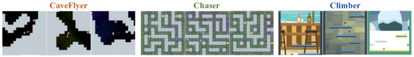
Figure 20: Examples of three games with different structures. As shown in Table 4, the most effective augmentations are color jitter, rotation and cropping for Climber, CaveFlyer and Chaser, respectively.

5.3.2 Vision Generalization on DMControl-GB

As a variant of the DeepMind control suite [10], DMControl-GB [53] aims to evaluate the generalization ability of an agent by changing the image color or replacing the background with another image set (Figure 19). A comparison of performance levels achieved in seen environments (Table 2) and unseen environments (Table 5) shows that although DrQ [13] is prominent in terms of sample efficiency, the diversity derived from the naive application of cropping is limited, and a significant generalization gap is induced when this approach is transferred to unseen environments. To provide sufficient visual diversity for generalization, it is necessary to use strong augmentations such as random convolution and overlay, as indicated by the results of follow-up studies.

Table 5: Evaluation of Generalization Ability on DMControl-GB. The scores (means and standard deviations) are obtained by conducting training in a fixed environment and performing evaluations in two unseen test environments with random colors (top) and natural video backgrounds (bottom).

DMControl-GB	SAC	CURL	RAD	PAD	DrQ	SVEA	SODA	SIM	TLDA	SECANT	PIE-G
(Random Colors)	[17]	[26]	[12]	[156]	[13]	[15]	[53]	[137]	[81]	[48]	[42]
Walker,	$365$	$662$	$644$	$797$	$770$	$942$	$930$	$940$	${\color[rgb]{0.75390625,0,0}\bm{947}}$	$939$	$941$
Stand	$\pm 79$	$\pm 54$	$\pm 88$	$\pm 46$	$\pm 71$	$\pm 26$	$\pm 12$	$\pm 2$	${\color[rgb]{0.75390625,0,0}{\pm 26}}$	$\pm 7$	$\pm 35$
Walker,	$144$	$445$	$400$	$468$	$520$	$760$	$697$	$803$	$823$	$856$	${\color[rgb]{0.75390625,0,0}\bm{884}}$
Walk	$\pm 19$	$\pm 99$	$\pm 61$	$\pm 47$	$\pm 91$	$\pm 145$	$\pm 66$	$\pm 33$	$\pm 58$	$\pm 31$	${\color[rgb]{0.75390625,0,0}{\pm 20}}$
Cartpole,	$248$	$454$	$590$	$837$	$630$	$837$	$831$	$841$	$760$	${\color[rgb]{0.75390625,0,0}\bm{866}}$	$749$
Swingup	$\pm 24$	$\pm 110$	$\pm 53$	$\pm 63$	$\pm 52$	$\pm 23$	$\pm 21$	$\pm 13$	$\pm 60$	${\color[rgb]{0.75390625,0,0}{\pm 15}}$	$\pm 46$
Ball in cup,	$151$	$231$	$541$	$563$	$365$	${\color[rgb]{0.75390625,0,0}\bm{961}}$	$949$	$953$	$932$	$958$	${\color[rgb]{0.75390625,0,0}\bm{964}}$
Catch	$\pm 36$	$\pm 92$	$\pm 29$	$\pm 50$	$\pm 210$	${\color[rgb]{0.75390625,0,0}{\pm 7}}$	$\pm 19$	$\pm 7$	$\pm 32$	$\pm 7$	${\color[rgb]{0.75390625,0,0}{\pm 7}}$
Finger,	$504$	$691$	$667$	$803$	$776$	${\color[rgb]{0.75390625,0,0}\bm{977}}$	$793$	$960$	$-$	$910$	$-$
Spin	$\pm 114$	$\pm 12$	$\pm 154$	$\pm 72$	$\pm 134$	${\color[rgb]{0.75390625,0,0}{\pm 5}}$	$\pm 128$	$\pm 6$		$\pm 115$
Cheetah,	$133$	$-$	$-$	$159$	$100$	$273$	$294$	$-$	$371$	${\color[rgb]{0.75390625,0,0}\bm{582}}$	$364$
Run	$\pm 26$			$\pm 28$	$\pm 27$	$\pm 23$	$\pm 34$		$\pm 51$	${\color[rgb]{0.75390625,0,0}{\pm 64}}$	$\pm 40$
(Natural Videos)
Walker,	$274$	$852$	$745$	$935$	$873$	$961$	$955$	$963$	${\color[rgb]{0.75390625,0,0}\bm{973}}$	$932$	$957$
Stand	$\pm 39$	$\pm 75$	$\pm 146$	$\pm 20$	$\pm 83$	$\pm 8$	$\pm 13$	$\pm 5$	${\color[rgb]{0.75390625,0,0}{\pm 6}}$	$\pm 15$	$\pm 12$
Walker,	$104$	$556$	$606$	$717$	$682$	$819$	$768$	$861$	${\color[rgb]{0.75390625,0,0}\bm{873}}$	$842$	${\color[rgb]{0.75390625,0,0}\bm{870}}$
Walk	$\pm 14$	$\pm 133$	$\pm 63$	$\pm 79$	$\pm 89$	$\pm 71$	$\pm 38$	$\pm 33$	${\color[rgb]{0.75390625,0,0}{\pm 34}}$	$\pm 47$	${\color[rgb]{0.75390625,0,0}\bm{\pm 22}}$
Cartpole,	$204$	$404$	$373$	$521$	$485$	${\color[rgb]{0.75390625,0,0}\bm{782}}$	$758$	$770$	$671$	$752$	$597$
Swingup	$\pm 20$	$\pm 67$	$\pm 72$	$\pm 76$	$\pm 105$	${\color[rgb]{0.75390625,0,0}{\pm 27}}$	$\pm 62$	$\pm 13$	$\pm 57$	$\pm 38$	$\pm 61$
Ball in cup,	$172$	$316$	$481$	$436$	$318$	$871$	$875$	$820$	$887$	$903$	${\color[rgb]{0.75390625,0,0}\bm{922}}$
Catch	$\pm 46$	$\pm 119$	$\pm 26$	$\pm 55$	$\pm 157$	$\pm 106$	$\pm 56$	$\pm 135$	$\pm 58$	$\pm 49$	${\color[rgb]{0.75390625,0,0}{\pm 20}}$
Finger,	$276$	$502$	$400$	$691$	$533$	$808$	$695$	$81$	$-$	${\color[rgb]{0.75390625,0,0}\bm{861}}$	$837$
Spin	$\pm 81$	$\pm 19$	$\pm 64$	$\pm 80$	$\pm 119$	$\pm 33$	$\pm 94$	$\pm 38$		${\color[rgb]{0.75390625,0,0}{\pm 102}}$	$\pm 107$
Cheetah,	$80$	$-$	$-$	$206$	$102$	$292$	$229$	$-$	$356$	${\color[rgb]{0.75390625,0,0}\bm{428}}$	$287$
Run	$\pm 19$			$\pm 34$	$\pm 30$	$\pm 32$	$\pm 29$		$\pm 52$	${\color[rgb]{0.75390625,0,0}{\pm 70}}$	$\pm 20$

SVEA [15] and TLDA [81] both significantly outperform DrQ [13] by focusing on stabilizing the training process when leveraging strong augmentation to optimize the representation and policy together. Another way to improve generalization is to decouple the unsupervised representation learning and the RL optimization process, either in an iterative manner (e.g., SODA [53] and SIM [137]) or in a sequential manner (e.g., SECANT [48]). Moreover, pre-trained encoders from off-the-shelf image datasets such as PIE-G [42] from ImageNet [74] also show attractive potential to provide generalizable representations in downstream tasks.

6 Discussion and Future Works

DA techniques have greatly improved the sample efficiency and generalization abilities of visual RL methods, yet many challenges remain to be addressed. In this section, we elaborate on these points and highlight the key directions for future research, including the opportunities, limitations, and theoretical foundations of DA in visual RL.

6.1 Semantic-Level DA

DA implicitly regularizes a model by introducing prior inductive bias into the given dataset. It can be considered as a kind of feature manipulation technique that essentially changes the relative contributions of task-relevant and task-irrelevant features in the gradient update steps of the utilized network [84]. In this way, a perfect (but unrealistic) DA method is expected to work at the semantic level: capable of identifying features that are relevant to the current label or task and eliminating the rest. While label-preserving transformations in SL and optimality-invariant transformations in RL rely on the above assumption, it is challenging to implement pixel-level augmentations that transform each pixel in a context-agnostic manner [81]. Consequently, these pixel-level manipulations severely limit the effectiveness of DA, especially in visual RL. Hence, an exciting direction for further leveraging DA is to develop semantic-level augmentation manipulations instead of pixel-level manipulations.

For example, the motivation of EXPAND [123] and TLDA [81] in Section 3.6 is to prevent the salient or flimsy areas of observed images from being augmented. In the computer vision community, KeepAugment [124] uses a saliency map to identify the key regions and then preserves these informative regions during augmentation to produce reliable training samples. In addition to DA, VAI [5] employs unsupervised keypoint detection and visual attention in combination with a reconstruction loss to force the encoder to embed only the foreground information of the input image as an inductive bias.

6.2 Trade-off Between Instability and Generalization

In practice, DrQ [13] and RAD [12] combined with random cropping, as implicit regularization methods, can yield significantly improved sample efficiency during training, while a noticeable generalization gap is observed when these approaches are transferred to unseen environments [53, 15, 48]. Furthermore, more diverse augmentations, such as color jitter, have the potential to improve generalization but tend to result in unstable optimization and poor sample efficiency [12, 15]. Therefore, a dilemma of balancing between stability and generalization is persistent when applying DA in visual RL due to its fragile optimization process [48].

This dilemma is often ascribed to the fact that policy optimization and representation learning are conflated in current end-to-end visual RL algorithms [48, 53]. As a result, it makes sense to separate them by independently learning a robust representation and a competent policy, as discussed in Section 4.3 and Section 4.4. Decoupling enables generalization improvements to be induced by heavy augmentations while ensuring satisfactory sample efficiency through weak augmentations [53, 48]. Additionally, this dilemma is also caused by the pixel-level augmentation techniques, which may inevitably destroy critical features when the augmentations become heavy.

Further insight lies in the bias-variance trade-off, which is the core tenet of machine learning [157]. Current complex models such as DNNs generally have low bias but suffer from high variance. This implies that these models are likely to overfit the training data and achieve poor performance on unseen data. With increased diversity, DA reduces variance by making the associated model more general with an improved ability to generalize [16]. Although DA may mitigate the issue of overfitting, certain augmentation combinations can actually lead to underfitting, making the training process unstable and challenging [83, 126]. Note that the issue of underfitting is more detrimental in RL, as its optimization process is more unstable than those of supervised tasks.

6.3 DA: Supervised Learning (SL) vs. RL

In view of the success of DA in SL, such as image classification tasks [94, 158], a growing amount of effort has been devoted to leveraging DA in the RL community [12, 23, 40]. However, augmentation techniques in the domain of SL are unlikely to be fully applicable to RL settings. In practice, certain distinct differences are present between visual RL and SL in terms of DA.

First, as opposed to supervised tasks such as image classification, where heavy transformations such as Mixup [94] and CutMix [97] possess notable advantages over traditional image transformations, in visual RL, random cropping is the most practical augmentation technique [12, 54]. Hence, the augmented data harnessing approach must be thoughtfully designed to avoid causing potential harm to the optimization stability and to effectively exploit the generalization capabilities induced by DA [81]. Second, the timing of applying augmentation is critical in RL [159] but not in SL [160], as the time sensitivity of augmentation is more significant in RL. For instance, optimality-invariant augmentations such as cropping should be applied as early as possible to improve the sample efficiency and accelerate the RL training process. However, prior-based strong augmentations such as color jitter may interfere with RL training, so these techniques may be better adopted after RL optimization for knowledge distillation [159].

It is argued that the above differences are mainly due to the nonstationary nature of RL, especially compared with SL [48, 159]. Consequently, understanding the uniqueness of visual RL is pivotal to better leveraging DA, and it would be potentially fruitful for future work to revisit this difference from various views, such as information redundancy.

6.4 Theoretical Foundations for DA

In contrast to its widespread application in deep learning, DA has not yet received much attention in terms of its theoretical basis. Most recently, many attempts have been made to investigate the theoretical guarantees for DA from different perspectives; such guarantees are helpful for researchers to understand the practical effects of such approaches [83, 84, 161]. In this section, we provide a brief guide to previous works on the theoretical foundations of DA and summarize them into three categories: implicit regularization [126, 161, 80], invariance learning [83, 162] and feature manipulation [84, 163].

Implicit Regularization vs. Explicit Regularization.

Regularization is a fundamental technique in deep learning that aims to prevent overfitting and improve generalization abilities by constraining the complexity of a model [126, 164, 105]. The regularization strategies of DA act on the training data instead of the model’s parameters and hence can be considered a type of implicit regularization approach instead of an explicit regularization technique that imposes constraints on the parameters, such as minimizing the $\mathcal{L}_{2}$ norms of the parameters [161]. By keeping the parameter space intact, this data-driven regularization approach can maintain the model’s representational capacity while increasing its robustness [13, 80]. In fact, DA is more straightforward than explicit regularization that integrates the prior knowledge into objective functions, and neural networks can implicitly encode the attributes of DA without explicitly training towards these objectives [165]. Furthermore, attempts have also been made to derive explicit regularizers to describe the implicit regularization effect of DA [127].

Transformation Invariance.

Invariance is an essential property of all intelligent systems that makes them generalize effectively [166]. The purpose of DA is to constrain a model’s output to be invariant when applying task-irrelevant transformations to the input data [94, 54]. It has been widely accepted that translation invariance is an inherent feature of CNNs [165], whereas other types of transformation invariance, such as rotation invariance, must be induced by corresponding augmentations [82]. The definition of DA assumes that semantics are invariant to data transformation [51, 13], which implies that performing optimization with augmentation can result in implicit invariances. Furthermore, the specific details of augmentations can be used to encode prior knowledge about task-specific or dataset-specific invariances [166].

Feature Manipulation.

An alternative explanation of how DA works is derived from the perspective of feature manipulation [84]. Learning meaningful features from high-dimensional data is empirically challenging, as critical features are often highly sparse and associated with spurious features such as dense noise. In practice, this may result in the network’s overfitting the noisy features instead of properly learning the critical features [167]. First, by adjusting the relative contributions of the original data features, DA can effectively facilitate the incorporation of informative but hard-to-learn features into the learning process [84]. Second, the latest research shows that leveraging DA in contrastive learning can decouple spurious features from the representations of positive samples. By ignoring the decoupled features, the performance of networks may be boosted by focusing on the learning of resistant features [163].

As discussed in Section 6.3, distinct differences are observed between the applications of DA in (un)supervised learning and RL. However, the existing theoretical foundations of DA are mostly built on traditional tasks such as classification and regression. Hence, a principled understanding of this difference is in critical demand, and the development of theoretical foundations for DA in the paradigm of visual RL is imperative.

6.5 Limitations of DA

Although DA is a proven technique for accelerating the training process and improving the generalization ability of a model, its applications are highly task-specific and require extensive expert knowledge [54]. Recent theoretical studies have also suggested that DA may actually increase rather than reduce the uncertainty of estimates, which is contrary to commonly held beliefs [168]. Another dispute concerning DA is that it is essentially a cheating artifact relying on how benchmark environments collect and store data, which is not applicable in the real world [65]. In practice, DA works well when the variation between the training and test environments is known so that it can be reliably specified [55]. For example, in DMControl-GB, only visual settings such as background colors are varied in the test environments, and specific DA techniques, such as random convolution, can effectively capture these prior variations [15, 48].

7 Conclusion

In this paper, we present a comprehensive and systematic survey of DA in the paradigm of visual RL. We first propose High-Dimensional Contextual MDP (HCMDP) as a general framework of visual RL. Then, DA is introduced as a crucial factor for significantly improving the performance of agents, with a focus on their sample efficiency and generalization abilities. The structured experimental results obtained on widely used benchmarks further reveal the power and potential of these simple yet effective techniques in visual RL. This survey also provides a list of current challenges and potential directions for future studies. In the following, we present a few suggestions and insights that are intended to benefit the relevant communities.

1. Compact and robust representation is vital for acquiring sample-efficient and generalizable visual RL agents; therefore, it is necessary to apply appropriate representation learning strategies to tackle the specific challenges of visual RL (Section 2.2). As a data-driven technique, DA is an essential component of representation learning and has great potential to be further explored (Section 2.3).

2. To exploit the potential of DA, two orthogonal aspects need to be considered: how to augment data (Section 3) and how to effectively leverage augmented data (Section 4). The key motivation of these two aspects is to achieve semantic-level DA (Section 6.1) and attain an effective balance between the training stability and generalization ability of the utilized model (Section 6.2).

3. The difference between RL and SL should be given special attention when applying DA in visual RL, including fragile optimization process, the interactive data acquisition process and its absence of ground-truth labels (Section 6.3).

4. To understand the intrinsic role of DA and design DA-based methods in a more principled way, the development of rigorous theoretical foundations for DA in visual RL is urgently needed. Although several theoretical studies have been conducted on DA in SL, how to establish solid theoretical frameworks for DA in visual RL remains underexplored (Section 6.4).

Overall, this survey strives to provide the first unified and principled framework for the large body of thriving research on DA in visual RL. We expect it to serve as a valuable guide for researchers and practitioners, and stimulate more inspiration in this fascinating field.

References

- François-Lavet et al. [2018] Vincent François-Lavet, Peter Henderson, Riashat Islam, Marc G Bellemare, Joelle Pineau, et al. An introduction to deep reinforcement learning. Foundations and Trends® in Machine Learning, 11(3-4):219–354, 2018.
- Mnih et al. [2015] Volodymyr Mnih, Koray Kavukcuoglu, David Silver, Andrei A Rusu, Joel Veness, Marc G Bellemare, Alex Graves, Martin Riedmiller, Andreas K Fidjeland, Georg Ostrovski, et al. Human-level control through deep reinforcement learning. nature, 518(7540):529–533, 2015.
- Schulman et al. [2017] John Schulman, Filip Wolski, Prafulla Dhariwal, Alec Radford, and Oleg Klimov. Proximal policy optimization algorithms. arXiv preprint arXiv:1707.06347, 2017.
- Lillicrap et al. [2015] Timothy P Lillicrap, Jonathan J Hunt, Alexander Pritzel, Nicolas Heess, Tom Erez, Yuval Tassa, David Silver, and Daan Wierstra. Continuous control with deep reinforcement learning. arXiv preprint arXiv:1509.02971, 2015.
- Wang et al. [2021] Xudong Wang, Long Lian, and Stella X. Yu. Unsupervised visual attention and invariance for reinforcement learning. In Proceedings of the IEEE/CVF Conference on Computer Vision and Pattern Recognition (CVPR), pages 6677–6687, June 2021.
- Yarats et al. [2021a] Denis Yarats, Amy Zhang, Ilya Kostrikov, Brandon Amos, Joelle Pineau, and Rob Fergus. Improving sample efficiency in model-free reinforcement learning from images. In Proceedings of the AAAI Conference on Artificial Intelligence, volume 35, 2021a.
- Silver et al. [2018] David Silver, Thomas Hubert, Julian Schrittwieser, Ioannis Antonoglou, Matthew Lai, Arthur Guez, Marc Lanctot, Laurent Sifre, Dharshan Kumaran, Thore Graepel, et al. A general reinforcement learning algorithm that masters chess, shogi, and go through self-play. Science, 362, 2018.
- Kiran et al. [2021] B Ravi Kiran, Ibrahim Sobh, Victor Talpaert, Patrick Mannion, Ahmad A Al Sallab, Senthil Yogamani, and Patrick Pérez. Deep reinforcement learning for autonomous driving: A survey. IEEE Transactions on Intelligent Transportation Systems, 2021.
- Kalashnikov et al. [2018] Dmitry Kalashnikov, Alex Irpan, Peter Pastor, Julian Ibarz, Alexander Herzog, Eric Jang, Deirdre Quillen, Ethan Holly, Mrinal Kalakrishnan, Vincent Vanhoucke, et al. Scalable deep reinforcement learning for vision-based robotic manipulation. In Conference on Robot Learning. PMLR, 2018.
- Tassa et al. [2018] Yuval Tassa, Yotam Doron, Alistair Muldal, Tom Erez, Yazhe Li, Diego de Las Casas, David Budden, Abbas Abdolmaleki, Josh Merel, Andrew Lefrancq, et al. Deepmind control suite. arXiv preprint arXiv:1801.00690, 2018.
- Lee et al. [2020a] Alex X Lee, Anusha Nagabandi, Pieter Abbeel, and Sergey Levine. Stochastic latent actor-critic: Deep reinforcement learning with a latent variable model. Advances in Neural Information Processing Systems, 33:741–752, 2020a.
- Laskin et al. [2020a] Misha Laskin, Kimin Lee, Adam Stooke, Lerrel Pinto, Pieter Abbeel, and Aravind Srinivas. Reinforcement learning with augmented data. Advances in neural information processing systems, 33:19884–19895, 2020a.
- Yarats et al. [2020] Denis Yarats, Ilya Kostrikov, and Rob Fergus. Image augmentation is all you need: Regularizing deep reinforcement learning from pixels. In International Conference on Learning Representations, 2020.
- Yarats et al. [2021b] Denis Yarats, Rob Fergus, Alessandro Lazaric, and Lerrel Pinto. Mastering visual continuous control: Improved data-augmented reinforcement learning. In International Conference on Learning Representations, 2021b.
- Hansen et al. [2021] Nicklas Hansen, Hao Su, and Xiaolong Wang. Stabilizing deep q-learning with convnets and vision transformers under data augmentation. Advances in Neural Information Processing Systems, 34, 2021.
- Zhang et al. [2018a] Chiyuan Zhang, Oriol Vinyals, Remi Munos, and Samy Bengio. A study on overfitting in deep reinforcement learning. arXiv preprint arXiv:1804.06893, 2018a.
- Haarnoja et al. [2018] Tuomas Haarnoja, Aurick Zhou, Pieter Abbeel, and Sergey Levine. Soft actor-critic: Off-policy maximum entropy deep reinforcement learning with a stochastic actor. In International conference on machine learning, pages 1861–1870. PMLR, 2018.
- Cobbe et al. [2019] Karl Cobbe, Oleg Klimov, Chris Hesse, Taehoon Kim, and John Schulman. Quantifying generalization in reinforcement learning. In International Conference on Machine Learning. PMLR, 2019.
- Liu et al. [2020] Zhuang Liu, Xuanlin Li, Bingyi Kang, and Trevor Darrell. Regularization matters in policy optimization-an empirical study on continuous control. In International Conference on Learning Representations, 2020.
- Hausknecht and Wagener [2022] Matthew Hausknecht and Nolan Wagener. Consistent dropout for policy gradient reinforcement learning. arXiv preprint arXiv:2202.11818, 2022.
- Yu et al. [2022] Tao Yu, Zhizheng Zhang, Cuiling Lan, Zhibo Chen, and Yan Lu. Mask-based latent reconstruction for reinforcement learning. arXiv preprint arXiv:2201.12096, 2022.
- Lee et al. [2020b] Kuang-Huei Lee, Ian Fischer, Anthony Liu, Yijie Guo, Honglak Lee, John Canny, and Sergio Guadarrama. Predictive information accelerates learning in rl. Advances in Neural Information Processing Systems, 33:11890–11901, 2020b.
- Schwarzer et al. [2020] Max Schwarzer, Ankesh Anand, Rishab Goel, R Devon Hjelm, Aaron Courville, and Philip Bachman. Data-efficient reinforcement learning with self-predictive representations. In International Conference on Learning Representations, 2020.
- Yu et al. [2021] Tao Yu, Cuiling Lan, Wenjun Zeng, Mingxiao Feng, Zhizheng Zhang, and Zhibo Chen. Playvirtual: Augmenting cycle-consistent virtual trajectories for reinforcement learning. Advances in Neural Information Processing Systems, 34, 2021.
- Huang et al. [2022a] Tao Huang, Jiachen Wang, and Xiao Chen. Accelerating representation learning with view-consistent dynamics in data-efficient reinforcement learning. arXiv preprint arXiv:2201.07016, 2022a.
- Laskin et al. [2020b] Michael Laskin, Aravind Srinivas, and Pieter Abbeel. Curl: Contrastive unsupervised representations for reinforcement learning. In International Conference on Machine Learning, pages 5639–5650. PMLR, 2020b.
- Sun et al. [2022] Chenyu Sun, Hangwei Qian, and Chunyan Miao. Cclf: A contrastive-curiosity-driven learning framework for sample-efficient reinforcement learning. arXiv preprint arXiv:2205.00943, 2022.
- Kim et al. [2022] Minbeom Kim, Kyeongha Rho, Yong-duk Kim, and Kyomin Jung. Action-driven contrastive representation for reinforcement learning. Plos one, 17(3):e0265456, 2022.
- Fan and Li [2022] Jiameng Fan and Wenchao Li. Dribo: Robust deep reinforcement learning via multi-view information bottleneck. In International Conference on Machine Learning, pages 6074–6102. PMLR, 2022.
- Anand et al. [2019] Ankesh Anand, Evan Racah, Sherjil Ozair, Yoshua Bengio, Marc-Alexandre Côté, and R Devon Hjelm. Unsupervised state representation learning in atari. Advances in neural information processing systems, 2019.
- Nguyen et al. [2021] Thanh Nguyen, Tung M Luu, Thang Vu, and Chang D Yoo. Sample-efficient reinforcement learning representation learning with curiosity contrastive forward dynamics model. In 2021 IEEE/RSJ International Conference on Intelligent Robots and Systems (IROS), pages 3471–3477. IEEE, 2021.
- Zhu et al. [2022] Jinhua Zhu, Yingce Xia, Lijun Wu, Jiajun Deng, Wengang Zhou, Tao Qin, Tie-Yan Liu, and Houqiang Li. Masked contrastive representation learning for reinforcement learning. IEEE Transactions on Pattern Analysis and Machine Intelligence, 2022.
- Mazoure et al. [2020] Bogdan Mazoure, Remi Tachet des Combes, Thang Long Doan, Philip Bachman, and R Devon Hjelm. Deep reinforcement and infomax learning. In Advances in Neural Information Processing Systems, 2020.
- You et al. [2022] Bang You, Oleg Arenz, Youping Chen, and Jan Peters. Integrating contrastive learning with dynamic models for reinforcement learning from images. Neurocomputing, 2022.
- Hafner et al. [2019a] Danijar Hafner, Timothy Lillicrap, Ian Fischer, Ruben Villegas, David Ha, Honglak Lee, and James Davidson. Learning latent dynamics for planning from pixels. In International conference on machine learning, pages 2555–2565. PMLR, 2019a.
- Hafner et al. [2019b] Danijar Hafner, Timothy Lillicrap, Jimmy Ba, and Mohammad Norouzi. Dream to control: Learning behaviors by latent imagination. In International Conference on Learning Representations, 2019b.
- Hafner et al. [2020] Danijar Hafner, Timothy P Lillicrap, Mohammad Norouzi, and Jimmy Ba. Mastering atari with discrete world models. In International Conference on Learning Representations, 2020.
- Stooke et al. [2021] Adam Stooke, Kimin Lee, Pieter Abbeel, and Michael Laskin. Decoupling representation learning from reinforcement learning. In International Conference on Machine Learning, pages 9870–9879. PMLR, 2021.
- Yarats et al. [2021c] Denis Yarats, Rob Fergus, Alessandro Lazaric, and Lerrel Pinto. Reinforcement learning with prototypical representations. In International Conference on Machine Learning. PMLR, 2021c.
- Liu and Abbeel [2021a] Hao Liu and Pieter Abbeel. Behavior from the void: Unsupervised active pre-training. Advances in Neural Information Processing Systems, 34, 2021a.
- Laskin et al. [2022] Michael Laskin, Hao Liu, Xue Bin Peng, Denis Yarats, Aravind Rajeswaran, and Pieter Abbeel. Cic: Contrastive intrinsic control for unsupervised skill discovery. arXiv preprint arXiv:2202.00161, 2022.
- Yuan et al. [2022a] Zhecheng Yuan, Zhengrong Xue, Bo Yuan, Xueqian Wang, Yi Wu, Yang Gao, and Huazhe Xu. Pre-trained image encoder for generalizable visual reinforcement learning. In First Workshop on Pre-training: Perspectives, Pitfalls, and Paths Forward at ICML 2022, 2022a.
- Wang et al. [2022a] Che Wang, Xufang Luo, Keith Ross, and Dongsheng Li. Vrl3: A data-driven framework for visual deep reinforcement learning. arXiv preprint arXiv:2202.10324, 2022a.
- Parisi et al. [2022] Simone Parisi, Aravind Rajeswaran, Senthil Purushwalkam, and Abhinav Gupta. The unsurprising effectiveness of pre-trained vision models for control. arXiv preprint arXiv:2203.03580, 2022.
- Xiao et al. [2022] Tete Xiao, Ilija Radosavovic, Trevor Darrell, and Jitendra Malik. Masked visual pre-training for motor control. arXiv preprint arXiv:2203.06173, 2022.
- Shah and Kumar [2021] Rutav M Shah and Vikash Kumar. Rrl: Resnet as representation for reinforcement learning. In Proceedings of the 38th International Conference on Machine Learning, pages 9465–9476, 2021.
- Rakelly et al. [2021] Kate Rakelly, Abhishek Gupta, Carlos Florensa, and Sergey Levine. Which mutual-information representation learning objectives are sufficient for control? Advances in Neural Information Processing Systems, 34:26345–26357, 2021.
- Fan et al. [2021] Linxi Fan, Guanzhi Wang, De-An Huang, Zhiding Yu, Li Fei-Fei, Yuke Zhu, and Animashree Anandkumar. Secant: Self-expert cloning for zero-shot generalization of visual policies. In International Conference on Machine Learning, 2021.
- Wang et al. [2020a] Kaixin Wang, Bingyi Kang, Jie Shao, and Jiashi Feng. Improving generalization in reinforcement learning with mixture regularization. Advances in Neural Information Processing Systems, 2020a.
- Huang et al. [2021] Weiran Huang, Mingyang Yi, and Xuyang Zhao. Towards the generalization of contrastive self-supervised learning. arXiv preprint arXiv:2111.00743, 2021.
- Shorten and Khoshgoftaar [2019] Connor Shorten and Taghi M Khoshgoftaar. A survey on image data augmentation for deep learning. Journal of big data, 6(1):1–48, 2019.
- Feng et al. [2021] Steven Y Feng, Varun Gangal, Jason Wei, Sarath Chandar, Soroush Vosoughi, Teruko Mitamura, and Eduard Hovy. A survey of data augmentation approaches for nlp. arXiv preprint arXiv:2105.03075, 2021.
- Hansen and Wang [2021] Nicklas Hansen and Xiaolong Wang. Generalization in reinforcement learning by soft data augmentation. In 2021 IEEE International Conference on Robotics and Automation (ICRA), pages 13611–13617. IEEE, 2021.
- Raileanu et al. [2021] Roberta Raileanu, Maxwell Goldstein, Denis Yarats, Ilya Kostrikov, and Rob Fergus. Automatic data augmentation for generalization in reinforcement learning. Advances in Neural Information Processing Systems, 34:5402–5415, 2021.
- Kirk et al. [2021] Robert Kirk, Amy Zhang, Edward Grefenstette, and Tim Rocktäschel. A survey of generalisation in deep reinforcement learning. arXiv preprint arXiv:2111.09794, 2021.
- Song et al. [2019] Xingyou Song, Yiding Jiang, Stephen Tu, Yilun Du, and Behnam Neyshabur. Observational overfitting in reinforcement learning. In International Conference on Learning Representations, 2019.
- Tobin et al. [2017] Josh Tobin, Rachel Fong, Alex Ray, Jonas Schneider, Wojciech Zaremba, and Pieter Abbeel. Domain randomization for transferring deep neural networks from simulation to the real world. In 2017 IEEE/RSJ international conference on intelligent robots and systems (IROS). IEEE, 2017.
- Peng et al. [2018] Xue Bin Peng, Marcin Andrychowicz, Wojciech Zaremba, and Pieter Abbeel. Sim-to-real transfer of robotic control with dynamics randomization. In 2018 IEEE international conference on robotics and automation (ICRA), pages 3803–3810. IEEE, 2018.
- Muratore et al. [2022] Fabio Muratore, Theo Gruner, Florian Wiese, Boris Belousov, Michael Gienger, and Jan Peters. Neural posterior domain randomization. In Conference on Robot Learning, pages 1532–1542. PMLR, 2022.
- Du et al. [2019] Simon Du, Akshay Krishnamurthy, Nan Jiang, Alekh Agarwal, Miroslav Dudik, and John Langford. Provably efficient rl with rich observations via latent state decoding. In International Conference on Machine Learning, pages 1665–1674. PMLR, 2019.
- Han et al. [2021] Beining Han, Chongyi Zheng, Harris Chan, Keiran Paster, Michael Zhang, and Jimmy Ba. Learning domain invariant representations in goal-conditioned block mdps. Advances in Neural Information Processing Systems, 34, 2021.
- Ghosh et al. [2021] Dibya Ghosh, Jad Rahme, Aviral Kumar, Amy Zhang, Ryan P Adams, and Sergey Levine. Why generalization in rl is difficult: Epistemic pomdps and implicit partial observability. Advances in Neural Information Processing Systems, 34, 2021.
- Doshi-Velez and Konidaris [2016] Finale Doshi-Velez and George Konidaris. Hidden parameter markov decision processes: A semiparametric regression approach for discovering latent task parametrizations. In IJCAI: proceedings of the conference, volume 2016, page 1432. NIH Public Access, 2016.
- Hallak et al. [2015] Assaf Hallak, Dotan Di Castro, and Shie Mannor. Contextual markov decision processes. arXiv preprint arXiv:1502.02259, 2015.
- Tomar et al. [2021] Manan Tomar, Utkarsh A Mishra, Amy Zhang, and Matthew E Taylor. Learning representations for pixel-based control: What matters and why? arXiv preprint arXiv:2111.07775, 2021.
- Zhu et al. [2020] Yuke Zhu, Josiah Wong, Ajay Mandlekar, and Roberto Martín-Martín. robosuite: A modular simulation framework and benchmark for robot learning. arXiv preprint arXiv:2009.12293, 2020.
- Zhang et al. [2020a] Amy Zhang, Clare Lyle, Shagun Sodhani, Angelos Filos, Marta Kwiatkowska, Joelle Pineau, Yarin Gal, and Doina Precup. Invariant causal prediction for block mdps. In International Conference on Machine Learning, pages 11214–11224. PMLR, 2020a.
- Sodhani et al. [2022] Shagun Sodhani, Franziska Meier, Joelle Pineau, and Amy Zhang. Block contextual mdps for continual learning. In Learning for Dynamics and Control Conference, pages 608–623. PMLR, 2022.
- Hausknecht and Stone [2015] Matthew Hausknecht and Peter Stone. Deep recurrent q-learning for partially observable mdps. In 2015 aaai fall symposium series, 2015.
- Pan et al. [2022] Feiyang Pan, Tongzhe Zhang, Ling Luo, Jia He, and Shuoling Liu. Learn continuously, act discretely: Hybrid action-space reinforcement learning for optimal execution. In Proceedings of the Thirty-First International Joint Conference on Artificial Intelligence (IJCAI-22), pages 3912–3918, 2022.
- Yang et al. [2022a] Rui Yang, Jie Wang, Zijie Geng, Mingxuan Ye, Shuiwang Ji, Bin Li, and Feng Wu. Learning task-relevant representations for generalization via characteristic functions of reward sequence distributions. arXiv preprint arXiv:2205.10218, 2022a.
- Yu [2018] Yang Yu. Towards sample efficient reinforcement learning. In IJCAI, pages 5739–5743, 2018.
- Oord et al. [2018] Aaron van den Oord, Yazhe Li, and Oriol Vinyals. Representation learning with contrastive predictive coding. arXiv preprint arXiv:1807.03748, 2018.
- Deng et al. [2009] Jia Deng, Wei Dong, Richard Socher, Li-Jia Li, Kai Li, and Li Fei-Fei. Imagenet: A large-scale hierarchical image database. In 2009 IEEE conference on computer vision and pattern recognition, pages 248–255. Ieee, 2009.
- Krishnamurthy et al. [2016] Akshay Krishnamurthy, Alekh Agarwal, and John Langford. Pac reinforcement learning with rich observations. Advances in Neural Information Processing Systems, 29:1840–1848, 2016.
- Farebrother et al. [2018] Jesse Farebrother, Marlos C Machado, and Michael Bowling. Generalization and regularization in dqn. arXiv preprint arXiv:1810.00123, 2018.
- Igl et al. [2019] Maximilian Igl, Kamil Ciosek, Yingzhen Li, Sebastian Tschiatschek, Cheng Zhang, Sam Devlin, and Katja Hofmann. Generalization in reinforcement learning with selective noise injection and information bottleneck. Advances in neural information processing systems, 32, 2019.
- Zhang et al. [2020b] Amy Zhang, Rowan McAllister, Roberto Calandra, Yarin Gal, and Sergey Levine. Learning invariant representations for reinforcement learning without reconstruction. arXiv preprint arXiv:2006.10742, 2020b.
- Kemertas and Aumentado-Armstrong [2021] Mete Kemertas and Tristan Aumentado-Armstrong. Towards robust bisimulation metric learning. Advances in Neural Information Processing Systems, 34:4764–4777, 2021.
- Hernández-García and König [2018] Alex Hernández-García and Peter König. Data augmentation instead of explicit regularization. arXiv preprint arXiv:1806.03852, 2018.
- Yuan et al. [2022b] Zhecheng Yuan, Guozheng Ma, Yao Mu, Bo Xia, Bo Yuan, Xueqian Wang, Ping Luo, and Huazhe Xu. Don’t touch what matters: Task-aware lipschitz data augmentationfor visual reinforcement learning. arXiv preprint arXiv:2202.09982, 2022b.
- Immer et al. [2022] Alexander Immer, Tycho FA van der Ouderaa, Vincent Fortuin, Gunnar Rätsch, and Mark van der Wilk. Invariance learning in deep neural networks with differentiable laplace approximations. arXiv preprint arXiv:2202.10638, 2022.
- Botev et al. [2022] Aleksander Botev, Matthias Bauer, and Soham De. Regularising for invariance to data augmentation improves supervised learning. arXiv preprint arXiv:2203.03304, 2022.
- Shen et al. [2022a] Ruoqi Shen, Sébastien Bubeck, and Suriya Gunasekar. Data augmentation as feature manipulation: a story of desert cows and grass cows. arXiv preprint arXiv:2203.01572, 2022a.
- Yang et al. [2022b] Suorong Yang, Weikang Xiao, Mengcheng Zhang, Suhan Guo, Jian Zhao, and Furao Shen. Image data augmentation for deep learning: A survey. arXiv preprint arXiv:2204.08610, 2022b.
- DeVries and Taylor [2017a] Terrance DeVries and Graham W Taylor. Improved regularization of convolutional neural networks with cutout. arXiv preprint arXiv:1708.04552, 2017a.
- Khalifa et al. [2021] Nour Eldeen Khalifa, Mohamed Loey, and Seyedali Mirjalili. A comprehensive survey of recent trends in deep learning for digital images augmentation. Artificial Intelligence Review, pages 1–27, 2021.
- Mutasa et al. [2020] Simukayi Mutasa, Shawn Sun, and Richard Ha. Understanding artificial intelligence based radiology studies: What is overfitting? Clinical imaging, 65:96–99, 2020.
- Wong et al. [2016] Sebastien C Wong, Adam Gatt, Victor Stamatescu, and Mark D McDonnell. Understanding data augmentation for classification: when to warp? In 2016 international conference on digital image computing: techniques and applications (DICTA), pages 1–6. IEEE, 2016.
- Cubuk et al. [2019] Ekin D Cubuk, Barret Zoph, Dandelion Mane, Vijay Vasudevan, and Quoc V Le. Autoaugment: Learning augmentation strategies from data. In Proceedings of the IEEE/CVF Conference on Computer Vision and Pattern Recognition, pages 113–123, 2019.
- Lee et al. [2019] Kimin Lee, Kibok Lee, Jinwoo Shin, and Honglak Lee. Network randomization: A simple technique for generalization in deep reinforcement learning. arXiv preprint arXiv:1910.05396, 2019.
- Moreno-Barea et al. [2018] Francisco J Moreno-Barea, Fiammetta Strazzera, José M Jerez, Daniel Urda, and Leonardo Franco. Forward noise adjustment scheme for data augmentation. In 2018 IEEE symposium series on computational intelligence (SSCI), pages 728–734. IEEE, 2018.
- Zhang et al. [2020c] Linjun Zhang, Zhun Deng, Kenji Kawaguchi, Amirata Ghorbani, and James Zou. How does mixup help with robustness and generalization? arXiv preprint arXiv:2010.04819, 2020c.
- Zhang et al. [2017] Hongyi Zhang, Moustapha Cisse, Yann N Dauphin, and David Lopez-Paz. mixup: Beyond empirical risk minimization. arXiv preprint arXiv:1710.09412, 2017.
- Lin et al. [2014] Tsung-Yi Lin, Michael Maire, Serge Belongie, James Hays, Pietro Perona, Deva Ramanan, Piotr Dollár, and C Lawrence Zitnick. Microsoft coco: Common objects in context. In European conference on computer vision, pages 740–755. Springer, 2014.
- Zhong et al. [2017] Zhun Zhong, Liang Zheng, Guoliang Kang, Shaozi Li, and Yi Yang. Random erasing data augmentation. arXiv preprint arXiv:1708.04896, 2017.
- Yun et al. [2019] Sangdoo Yun, Dongyoon Han, Seong Joon Oh, Sanghyuk Chun, Junsuk Choe, and Youngjoon Yoo. Cutmix: Regularization strategy to train strong classifiers with localizable features. In Proceedings of the IEEE/CVF international conference on computer vision, pages 6023–6032, 2019.
- DeVries and Taylor [2017b] Terrance DeVries and Graham W Taylor. Dataset augmentation in feature space. arXiv preprint arXiv:1702.05538, 2017b.
- Cheung and Yeung [2020] Tsz-Him Cheung and Dit-Yan Yeung. Modals: Modality-agnostic automated data augmentation in the latent space. In International Conference on Learning Representations, 2020.
- Liu et al. [2018] Xiaofeng Liu, Yang Zou, Lingsheng Kong, Zhihui Diao, Junliang Yan, Jun Wang, Site Li, Ping Jia, and Jane You. Data augmentation via latent space interpolation for image classification. In 2018 24th International Conference on Pattern Recognition (ICPR), pages 728–733. IEEE, 2018.
- Ohno [2020] Hiroshi Ohno. Auto-encoder-based generative models for data augmentation on regression problems. Soft Computing, 24(11):7999–8009, 2020.
- Nair et al. [2018] Ashvin V Nair, Vitchyr Pong, Murtaza Dalal, Shikhar Bahl, Steven Lin, and Sergey Levine. Visual reinforcement learning with imagined goals. Advances in neural information processing systems, 31, 2018.
- Zhou et al. [2020] Kaiyang Zhou, Yongxin Yang, Yu Qiao, and Tao Xiang. Domain generalization with mixstyle. In International Conference on Learning Representations, 2020.
- Huang and Belongie [2017] Xun Huang and Serge Belongie. Arbitrary style transfer in real-time with adaptive instance normalization. In Proceedings of the IEEE international conference on computer vision, pages 1501–1510, 2017.
- Bertoin and Rachelson [2022] David Bertoin and Emmanuel Rachelson. Local feature swapping for generalization in reinforcement learning. arXiv preprint arXiv:2204.06355, 2022.
- Goodfellow et al. [2014] Ian J Goodfellow, Jonathon Shlens, and Christian Szegedy. Explaining and harnessing adversarial examples. arXiv preprint arXiv:1412.6572, 2014.
- Volpi et al. [2018] Riccardo Volpi, Hongseok Namkoong, Ozan Sener, John C Duchi, Vittorio Murino, and Silvio Savarese. Generalizing to unseen domains via adversarial data augmentation. Advances in neural information processing systems, 31, 2018.
- Zhang and Guo [2021] Hanping Zhang and Yuhong Guo. Generalization of reinforcement learning with policy-aware adversarial data augmentation. arXiv preprint arXiv:2106.15587, 2021.
- Choi et al. [2019] Jaehoon Choi, Taekyung Kim, and Changick Kim. Self-ensembling with gan-based data augmentation for domain adaptation in semantic segmentation. In Proceedings of the IEEE/CVF International Conference on Computer Vision, pages 6830–6840, 2019.
- Wang et al. [2022b] Zhen Wang, Liu Liu, Yiqun Duan, and Dacheng Tao. Continual learning through retrieval and imagination. Proceedings of the AAAI Conference on Artificial Intelligence, 2022b.
- Mansourifar et al. [2019] Hadi Mansourifar, Lin Chen, and Weidong Shi. Virtual big data for gan based data augmentation. In 2019 IEEE International Conference on Big Data (Big Data), pages 1478–1487. IEEE, 2019.
- Gamrian and Goldberg [2019] Shani Gamrian and Yoav Goldberg. Transfer learning for related reinforcement learning tasks via image-to-image translation. In International Conference on Machine Learning, pages 2063–2072. PMLR, 2019.
- Chepurko et al. [2020] Nadiia Chepurko, Ryan Marcus, Emanuel Zgraggen, Raul Castro Fernandez, Tim Kraska, and David Karger. Arda: automatic relational data augmentation for machine learning. Proceedings of the VLDB Endowment, 2020.
- Li et al. [2020] Yonggang Li, Guosheng Hu, Yongtao Wang, Timothy Hospedales, Neil M Robertson, and Yongxin Yang. Differentiable automatic data augmentation. In European Conference on Computer Vision, pages 580–595. Springer, 2020.
- Auer [2002] Peter Auer. Using confidence bounds for exploitation-exploration trade-offs. Journal of Machine Learning Research, 3(Nov):397–422, 2002.
- Gil et al. [2021] Yoonhee Gil, Jongchan Baek, Jonghyuk Park, and Soohee Han. Automatic data augmentation by upper confidence bounds for deep reinforcement learning. In 2021 21st International Conference on Control, Automation and Systems (ICCAS), pages 1199–1203. IEEE, 2021.
- Wang et al. [2016a] Jane X Wang, Zeb Kurth-Nelson, Dhruva Tirumala, Hubert Soyer, Joel Z Leibo, Remi Munos, Charles Blundell, Dharshan Kumaran, and Matt Botvinick. Learning to reinforcement learn. arXiv preprint arXiv:1611.05763, 2016a.
- Finn et al. [2017] Chelsea Finn, Pieter Abbeel, and Sergey Levine. Model-agnostic meta-learning for fast adaptation of deep networks. In International conference on machine learning, pages 1126–1135. PMLR, 2017.
- Chen et al. [2022] Chaoqi Chen, Jiongcheng Li, Xiaoguang Han, Xiaoqing Liu, and Yizhou Yu. Compound domain generalization via meta-knowledge encoding. In 2022 IEEE/CVF Conference on Computer Vision and Pattern Recognition (CVPR), pages 7109–7119, 2022. doi: 10.1109/CVPR52688.2022.00698.
- Greydanus et al. [2018] Samuel Greydanus, Anurag Koul, Jonathan Dodge, and Alan Fern. Visualizing and understanding atari agents. In International conference on machine learning, pages 1792–1801. PMLR, 2018.
- Mott et al. [2019] Alexander Mott, Daniel Zoran, Mike Chrzanowski, Daan Wierstra, and Danilo Jimenez Rezende. Towards interpretable reinforcement learning using attention augmented agents. Advances in Neural Information Processing Systems, 32, 2019.
- Zhang et al. [2019] Ruohan Zhang, Faraz Torabi, Lin Guan, Dana H Ballard, and Peter Stone. Leveraging human guidance for deep reinforcement learning tasks. arXiv preprint arXiv:1909.09906, 2019.
- Guan et al. [2021] Lin Guan, Mudit Verma, Sihang Guo, Ruohan Zhang, and Subbarao Kambhampati. Widening the pipeline in human-guided reinforcement learning with explanation and context-aware data augmentation. Advances in Neural Information Processing Systems, 2021.
- Gong et al. [2021] Chengyue Gong, Dilin Wang, Meng Li, Vikas Chandra, and Qiang Liu. Keepaugment: A simple information-preserving data augmentation approach. In Proceedings of the IEEE/CVF Conference on Computer Vision and Pattern Recognition, pages 1055–1064, 2021.
- Laskin et al. [2021] Michael Laskin, Denis Yarats, Hao Liu, Kimin Lee, Albert Zhan, Kevin Lu, Catherine Cang, Lerrel Pinto, and Pieter Abbeel. Urlb: Unsupervised reinforcement learning benchmark. arXiv preprint arXiv:2110.15191, 2021.
- Moradi et al. [2020] Reza Moradi, Reza Berangi, and Behrouz Minaei. A survey of regularization strategies for deep models. Artificial Intelligence Review, 53(6):3947–3986, 2020.
- Balestriero et al. [2022a] Randall Balestriero, Ishan Misra, and Yann LeCun. A data-augmentation is worth a thousand samples: Exact quantification from analytical augmented sample moments. arXiv preprint arXiv:2202.08325, 2022a.
- Yang et al. [2022c] Shuo Yang, Yijun Dong, Rachel Ward, Inderjit S Dhillon, Sujay Sanghavi, and Qi Lei. Sample efficiency of data augmentation consistency regularization. arXiv preprint arXiv:2202.12230, 2022c.
- Zhang and Ma [2022] Junbo Zhang and Kaisheng Ma. Rethinking the augmentation module in contrastive learning: Learning hierarchical augmentation invariance with expanded views. In Proceedings of the IEEE/CVF Conference on Computer Vision and Pattern Recognition, 2022.
- Von Kügelgen et al. [2021] Julius Von Kügelgen, Yash Sharma, Luigi Gresele, Wieland Brendel, Bernhard Schölkopf, Michel Besserve, and Francesco Locatello. Self-supervised learning with data augmentations provably isolates content from style. Advances in Neural Information Processing Systems, 34, 2021.
- Cobbe et al. [2020] Karl Cobbe, Chris Hesse, Jacob Hilton, and John Schulman. Leveraging procedural generation to benchmark reinforcement learning. In International conference on machine learning. PMLR, 2020.
- He et al. [2021a] Tairan He, Yuge Zhang, Kan Ren, Che Wang, Weinan Zhang, Dongsheng Li, and Yuqing Yang. Aarl: Automated auxiliary loss for reinforcement learning. openreview.net, 2021a.
- Bellemare et al. [2019] Marc Bellemare, Will Dabney, Robert Dadashi, Adrien Ali Taiga, Pablo Samuel Castro, Nicolas Le Roux, Dale Schuurmans, Tor Lattimore, and Clare Lyle. A geometric perspective on optimal representations for reinforcement learning. Advances in neural information processing systems, 32, 2019.
- Rafiee et al. [2022] Banafsheh Rafiee, Jun Jin, Jun Luo, and Adam White. What makes useful auxiliary tasks in reinforcement learning: investigating the effect of the target policy. arXiv preprint arXiv:2204.00565, 2022.
- Li et al. [2022] Xiang Li, Jinghuan Shang, Srijan Das, and Michael S Ryoo. Does self-supervised learning really improve reinforcement learning from pixels? arXiv preprint arXiv:2206.05266, 2022.
- He et al. [2022] Tairan He, Yuge Zhang, Kan Ren, Minghuan Liu, Che Wang, Weinan Zhang, Yuqing Yang, and Dongsheng Li. Reinforcement learning with automated auxiliary loss search. arXiv preprint arXiv:2210.06041, 2022.
- Wu et al. [2022] Keyu Wu, Min Wu, Zhenghua Chen, Yuecong Xu, and Xiaoli Li. Generalizing reinforcement learning through fusing self-supervised learning into intrinsic motivation. The 36th AAAI Conference on Artificial Intelligence (AAAI 2022), 2022.
- Tschannen et al. [2019] Michael Tschannen, Josip Djolonga, Paul K Rubenstein, Sylvain Gelly, and Mario Lucic. On mutual information maximization for representation learning. arXiv preprint arXiv:1907.13625, 2019.
- Federici et al. [2020] Marco Federici, Anjan Dutta, Patrick Forré, Nate Kushman, and Zeynep Akata. Learning robust representations via multi-view information bottleneck. arXiv preprint arXiv:2002.07017, 2020.
- He et al. [2020] Kaiming He, Haoqi Fan, Yuxin Wu, Saining Xie, and Ross Girshick. Momentum contrast for unsupervised visual representation learning. In Proceedings of the IEEE/CVF Conference on Computer Vision and Pattern Recognition (CVPR), June 2020.
- Hendrycks et al. [2019] Dan Hendrycks, Norman Mu, Ekin D Cubuk, Barret Zoph, Justin Gilmer, and Balaji Lakshminarayanan. Augmix: A simple data processing method to improve robustness and uncertainty. arXiv preprint arXiv:1912.02781, 2019.
- He et al. [2021b] Kaiming He, Xinlei Chen, Saining Xie, Yanghao Li, Piotr Dollár, and Ross Girshick. Masked autoencoders are scalable vision learners. arXiv preprint arXiv:2111.06377, 2021b.
- Brown et al. [2020] Tom Brown, Benjamin Mann, Nick Ryder, Melanie Subbiah, Jared D Kaplan, Prafulla Dhariwal, Arvind Neelakantan, Pranav Shyam, Girish Sastry, Amanda Askell, et al. Language models are few-shot learners. Advances in neural information processing systems, 33:1877–1901, 2020.
- Wang et al. [2022c] Zhen Wang, Liu Liu, Yiqun Duan, and Dacheng Tao. Sin: Semantic inference network for few-shot streaming label learning. IEEE Transactions on Neural Networks and Learning Systems, pages 1–14, 2022c. doi: 10.1109/TNNLS.2022.3162747.
- Hansen et al. [2019] Steven Hansen, Will Dabney, Andre Barreto, Tom Van de Wiele, David Warde-Farley, and Volodymyr Mnih. Fast task inference with variational intrinsic successor features. arXiv preprint arXiv:1906.05030, 2019.
- Liu and Abbeel [2021b] Hao Liu and Pieter Abbeel. Aps: Active pretraining with successor features. In International Conference on Machine Learning, pages 6736–6747. PMLR, 2021b.
- Schwarzer et al. [2021] Max Schwarzer, Nitarshan Rajkumar, Michael Noukhovitch, Ankesh Anand, Laurent Charlin, R Devon Hjelm, Philip Bachman, and Aaron C Courville. Pretraining representations for data-efficient reinforcement learning. Advances in Neural Information Processing Systems, 34, 2021.
- Kaiser et al. [2019] Lukasz Kaiser, Mohammad Babaeizadeh, Piotr Milos, Blazej Osinski, Roy H Campbell, Konrad Czechowski, Dumitru Erhan, Chelsea Finn, Piotr Kozakowski, Sergey Levine, et al. Model-based reinforcement learning for atari. arXiv preprint arXiv:1903.00374, 2019.
- Shen et al. [2022b] Li Shen, Long Yang, Shixiang Chen, Bo Yuan, Xueqian Wang, Dacheng Tao, et al. Penalized proximal policy optimization for safe reinforcement learning. arXiv preprint arXiv:2205.11814, 2022b.
- Beattie et al. [2016] Charles Beattie, Joel Z Leibo, Denis Teplyashin, Tom Ward, Marcus Wainwright, Heinrich Küttler, Andrew Lefrancq, Simon Green, Víctor Valdés, Amir Sadik, et al. Deepmind lab. arXiv preprint arXiv:1612.03801, 2016.
- Stone et al. [2021] Austin Stone, Oscar Ramirez, Kurt Konolige, and Rico Jonschkowski. The distracting control suite–a challenging benchmark for reinforcement learning from pixels. arXiv preprint arXiv:2101.02722, 2021.
- Grigsby and Qi [2020] Jake Grigsby and Yanjun Qi. Measuring visual generalization in continuous control from pixels. arXiv preprint arXiv:2010.06740, 2020.
- Zhang et al. [2018b] Amy Zhang, Yuxin Wu, and Joelle Pineau. Natural environment benchmarks for reinforcement learning. arXiv preprint arXiv:1811.06032, 2018b.
- Wang et al. [2016b] Ziyu Wang, Tom Schaul, Matteo Hessel, Hado Hasselt, Marc Lanctot, and Nando Freitas. Dueling network architectures for deep reinforcement learning. In International conference on machine learning, pages 1995–2003. PMLR, 2016b.
- Wang et al. [2022d] Zhen Wang, Liu Liu, Yiqun Duan, Yajing Kong, and Dacheng Tao. Continual learning with lifelong vision transformer. In Proceedings of the IEEE/CVF Conference on Computer Vision and Pattern Recognition (CVPR), pages 171–181, June 2022d.
- Hansen et al. [2020] Nicklas Hansen, Rishabh Jangir, Yu Sun, Guillem Alenyà, Pieter Abbeel, Alexei A Efros, Lerrel Pinto, and Xiaolong Wang. Self-supervised policy adaptation during deployment. arXiv preprint arXiv:2007.04309, 2020.
- Dietterich [1995] Tom Dietterich. Overfitting and undercomputing in machine learning. ACM computing surveys (CSUR), 27(3):326–327, 1995.
- Krizhevsky et al. [2012] Alex Krizhevsky, Ilya Sutskever, and Geoffrey E Hinton. Imagenet classification with deep convolutional neural networks. Advances in neural information processing systems, 25:1097–1105, 2012.
- Ko and Ok [2021] Byungchan Ko and Jungseul Ok. Time matters in using data augmentation for vision-based deep reinforcement learning. arXiv preprint arXiv:2102.08581, 2021.
- Golatkar et al. [2019] Aditya Sharad Golatkar, Alessandro Achille, and Stefano Soatto. Time matters in regularizing deep networks: Weight decay and data augmentation affect early learning dynamics, matter little near convergence. Advances in Neural Information Processing Systems, 2019.
- Balestriero et al. [2022b] Randall Balestriero, Leon Bottou, and Yann LeCun. The effects of regularization and data augmentation are class dependent. arXiv preprint arXiv:2204.03632, 2022b.
- Mei et al. [2021] Song Mei, Theodor Misiakiewicz, and Andrea Montanari. Learning with invariances in random features and kernel models. In Conference on Learning Theory, pages 3351–3418. PMLR, 2021.
- Wen and Li [2021] Zixin Wen and Yuanzhi Li. Toward understanding the feature learning process of self-supervised contrastive learning. In International Conference on Machine Learning. PMLR, 2021.
- Wang et al. [2020b] Zhen Wang, Liu Liu, and Dacheng Tao. Deep streaming label learning. In International Conference on Machine Learning (ICML), volume 119, pages 9963–9972, 2020b.
- Yan and Huang [2021] Eddie Yan and Yanping Huang. Do cnns encode data augmentations? In 2021 International Joint Conference on Neural Networks (IJCNN), pages 1–8. IEEE, 2021.
- Benton et al. [2020] Gregory Benton, Marc Finzi, Pavel Izmailov, and Andrew Gordon Wilson. Learning invariances in neural networks. Advances in Neural Information Processing Systems, 2020, 2020.
- Nozawa and Sato [2022] Kento Nozawa and Issei Sato. Empirical evaluation and theoretical analysis for representation learning: A survey. arXiv preprint arXiv:2204.08226, 2022.
- Huang et al. [2022b] Kevin H Huang, Peter Orbanz, and Morgane Austern. Quantifying the effects of data augmentation. arXiv preprint arXiv:2202.09134, 2022b.