Abstract

When proxies (external instruments) used to identify target structural shocks are weak, inference in proxy-SVARs (SVAR-IVs) is nonstandard and the construction of asymptotically valid confidence sets for the impulse responses of interest requires weak-instrument robust methods. In the presence of multiple target shocks, test inversion techniques require extra restrictions on the proxy-SVAR parameters other those implied by the proxies that may be difficult to interpret and test. We show that frequentist asymptotic inference in these situations can be conducted through Minimum Distance estimation and standard asymptotic methods if the proxy-SVAR can be identified by using ‘strong’ instruments for the non-target shocks; i.e. the shocks which are not of primary interest in the analysis. The suggested identification strategy hinges on a novel pre-test for the null of instrument relevance based on bootstrap resampling which is not subject to pre-testing issues. Specifically, the validity of post-test asymptotic inferences remains unaffected by the test outcomes due to an asymptotic independence result between the bootstrap and non-bootstrap statistics. The test is robust to conditionally heteroskedastic and/or zero-censored proxies, is computationally straightforward and applicable regardless of the number of shocks being instrumented. Some illustrative examples show the empirical usefulness of the suggested identification and testing strategy.

Keywords: Proxy-SVAR, Bootstrap inference, external instruments, identification, oil supply shock.

JEL Classification: C32, C51, C52, E44

1 Introduction

Proxy-SVARs, or SVAR-IVs, popularized by Stock (2008), Stock and Watson (2012, 2018) and Mertens and Ravn (2013), have become standard tools to track the dynamic causal effects produced by macroeconomic shocks on variables of interest. In proxy-SVARs, the model is complemented with ‘external’ variables – which we call ‘proxies’, ‘instruments’ or ‘external variables’ interchangeably; such variables carry information on the structural shocks of interest, the target shocks, and allow to disregard the structural shocks not of primary interest in the analysis, the non-target shocks. Recent contributions on frequentist inference in proxy-SVARs include Montiel Olea, Stock and Watson (2021) and Jentsch and Lunsford (2022); in the Bayesian framework, Arias, Rubio-Ramirez and Waggoner (2021) and Giacomini, Kitagawa and Read (2022) discuss inference in the case of set-identification.

Inference in proxy-SVARs depends on whether the proxies are strongly or weakly correlated with the target shocks. If the connection between the proxies and the target shocks is ‘local-to-zero’, as in Staiger and Stock (1997) and Stock and Yogo (2005), asymptotic inference is non-standard. In such case, weak-proxy robust methods can be obtained by extending the logic of Anderson-Rubin tests (Anderson and Rubin, 1949), see Montiel Olea et al. (2021). Grid Moving Block Bootstrap Anderson-Rubin confidence sets (‘grid MBB AR’) for normalized impulse response functions [IRFs] (Brüggemann, Jentsch and Trenkler, 2016; Jentsch and Lunsford, 2019) can also be applied in the special case where one proxy identifies one structural shock; see Jentsch and Lunsford (2022).

When proxy-SVARs feature multiple target shocks, further inferential difficulties arise. First, (point-)identification requires additional restrictions, other than those provided by the instruments; see Mertens and Ravn (2013), Angelini and Fanelli (2019), Arias et al. (2021), Montiel Olea et al. (2021) and Giacomini et al. (2022). Second, in the frequentist setup the implementation of weak-instrument robust inference as in Montiel Olea et al. (2021) may imply a large number of additional restrictions on the parameters of the proxy-SVAR relative to those needed under strong proxies. These extra restrictions are not always credible, and may be difficult to test; see Montiel Olea et al. (2021, Section A.7) and Section S.9 of our supplement. Fourth, the theory for the grid bootstrap Anderson-Rubin confidence sets does not extend to cases where multiple instruments identify multiple target shocks.

This paper is motivated by these inferential difficulties. In particular, we design an identification and (frequentist) estimation strategy intended to circumvent, when possible, the use of weak-instrument robust methods. The idea we pursue is to identify the proxy-SVAR through an ‘indirect’ approach, where a vector of proxies (say, $w_{t}$), correlated with (all or some of) the non-target shocks of the system and uncorrelated with the target shocks (say, $z_{t}$), is used to infer the IRFs of interest indirectly. We call this strategy ‘indirect identification strategy’ or ‘indirect-MD’ approach, as opposed to the conventional ‘direct’ approach based on instrumenting the target shock(s) directly with the (potentially weak) proxies $z_{t}$. As highlighted by our empirical illustrations, the indirect approach can prove more useful to a practitioner than one might think.

The proxies $w_{t}$ contribute to defining a set of moment conditions upon which we develop a novel Minimum Distance [MD] estimation approach (Newey and McFadden, 1994). We derive novel necessary order conditions and necessary and sufficient rank condition for the (local) identifiability of the proxy-SVAR. If the proxies $w_{t}$ are strong for the non-target shocks and the model is identified, asymptotically valid confidence intervals for the IRFs of interest obtain in the usual way; i.e., either by the delta-method or by bootstrap methods. Interestingly, the idea of using instruments for the non-target shocks to identify and infer the effects of structural shocks of interest was initially pursued via Bayesian methods in Caldara and Kamps (2017), where two fiscal (target) shocks are recovered by instrumenting the non-fiscal (non-target) shocks of the system. We defer to Section 5 a detailed comparison of our method with Caldara and Kamps (2017).

Key to the indirect identification strategy is the availability of strong proxies for the non-target shocks. In particular, it is essential that the investigator can screen ‘strong’ from ‘weak’ instruments, and that such screening does not affect post-test inference. To do so, we further contribute by designing a novel pre-test for strong against weak proxies based on bootstrap resampling.

Inspired by the idea originally developed in Angelini, Cavaliere and Fanelli (2022) for state-space models, we show that the bootstrap can be used to infer the strength of instruments, other than building valid confidence intervals for IRFs. In particular, we exploit the fact that under mild requirements, the MBB estimator of the proxy-SVAR parameters is asymptotically Gaussian when the instruments are strong while, under weak proxies à la Staiger and Stock (1997), the distribution of MBB estimator is random in the limit (in the sense of Cavaliere and Georgiev, 2020) and, in particular, is non-Gaussian. This allows to show that a test for the null of strong proxies can be designed as a normality test based on an appropriate number of bootstrap repetitions; such test is consistent against proxies which are weak in Staiger and Stock’s (1997). An idea that echoes this approach in the Bayesian setting can be found in Giacomini et al. (2022), who suggest using non-normality of the posterior distribution of a suitable function of proxy-SVAR parameters to diagnose the presence of weak proxies. This idea is not pursued further in their paper.

Our suggested test has several important features. First, it controls size under general conditions on VAR disturbances and proxies, including the case of conditional heteroskedasticity and/or zero-censored proxies. Second, with respect to extant tests such as Montiel Olea and Pflueger’s (2013) effective first-stage F-test for IV models with conditional heteroskedasticity, our test can be applied in the presence of multiple structural shocks; as far as we are aware, no test of strength for proxy-SVARs with multiple target shocks has been formalized in the literature. Third, it is computationally straightforward, as it boils down to running multivariate/univariate normality tests on the MBB replications of bootstrap estimators of the proxy-SVAR parameters. Fourth, it can be computed in the same way regardless of the number of shocks being instrumented. Fifth, and most importantly, the test does not affect second-stage inference, meaning that regardless of the outcome of the test, post-test inferences are not affected. This property marks an important difference relative to the literature on weak instrument asymptotics, where the negative consequences of pretesting the strength of proxies are well known and documented (see, inter alia, Zivot, Startz and Nelson, 1998; Hausman, Stock and Yogo, 2005; Andrews, Stock and Sun, 2019; Montiel Olea et al., 2021).

The paper is organized as follows. In Section 2 we motivate our approach with a simple illustrative example. In Section 3 we introduce the proxy-SVAR and rationalize the suggested identification strategy. The assumptions are summarized in Section 4, while we present our indirect-MD approach in Section 5. Section 6 deals with the novel approach to testing for strong proxies. To illustrate the practical implementation and relevance of our approach, we present in Section 7 two illustrative examples that reconsider models already estimated in the literature. Section 8 concludes. An accompanying supplement complements the paper along several dimensions, including auxiliary lemmas and their proofs, the proofs the propositions in the paper and an additional empirical illustration based on a fiscal proxy-SVAR.

2 Motivating example: a market (demand/supply) model

In this section we outline the main ideas in the paper by considering a ‘toy’ proxy-SVAR, where we omit the dynamics without loss of generality. We consider a model that comprises a demand and supply function for a good with associated structural shocks, given by the equations

$$\underset{Y_{t}}{\underbrace{\left(\begin{array}[]{c}q_{t}\\ p_{t}\end{array}\right)}}=\underset{B}{\underbrace{\left(\begin{array}[]{cc}\beta_{1,1}&\beta_{1,2}\\ \beta_{2,1}&\beta_{2,2}\end{array}\right)}}\underset{\varepsilon_{t}}{\underbrace{\left(\begin{array}[]{c}\varepsilon_{d,t}\\ \varepsilon_{s,t}\end{array}\right)}}\equiv\left(\begin{array}[]{c}\beta_{1,1}\varepsilon_{d,t}+\beta_{1,2}\varepsilon_{s,t}\\ \beta_{2,1}\varepsilon_{d,t}+\beta_{2,2}\varepsilon_{s,t}\end{array}\right)$$ (1)

where $q_{t}$ and $p_{t}$ are quantity and price at time $t$, respectively. The nonsingular matrix $B$ captures the instantaneous impact, on $Y_{t}:=(q_{t},p_{t})^{\prime}$, of the structural shocks $\varepsilon_{d,t},\varepsilon_{s,t}$, which are assumed to have unit variance and to be uncorrelated. We temporary (and conventionally) label $\varepsilon_{d,t}$ as the ‘demand shock’ and $\varepsilon_{s,t}$ as the ‘supply shock’, and assume that the objective of the analysis is the identification and estimation of the instantaneous impact of the demand shock on $Y_{t}$ through the ‘external variables’ approach. Hence, $\varepsilon_{d,t}$ is the target shock, $\varepsilon_{s,t}$ is the non-target shock, and the parameters of interest are the on-impact responses $\frac{\partial Y_{t}}{\partial\varepsilon_{d,t}}=B_{\bullet 1}:=(\beta_{1,1},\beta_{2,1})^{\prime}$; here $B_{\bullet 1}$ denotes the first column of $B$.

Since the two equations in (1) are essentially identical for arbitrary parameter values, nothing distinguishes a demand shock from a supply shock in the absence of further information/restrictions. The typical ‘direct approach’ to this partial identification problem is to consider an instrument $z_{t}$ correlated with the demand shock, ${E}(z_{t}\varepsilon_{d,t})=\phi\neq 0$ (relevance condition), and uncorrelated with the supply shock, ${E}(z_{t}\varepsilon_{s,t})=0$ (exogeneity condition). Now, consider the case where the investigator strongly suspects that $z_{t}$ is a weak proxy (meaning that $\phi$ can be ‘small’), but they also know that there exists an external variable $w_{t}$, correlated with the non-target supply shock and uncorrelated with the demand shock; formally, ${E}(w_{t}\varepsilon_{s,t})=\lambda\neq 0$ and ${E}(w_{t}\varepsilon_{d,t})=0$. Then, the proxy $w_{t}$ can be used to recover the parameters of interest (i.e., $B_{\bullet 1}$) ‘indirectly’; i.e., by instrumenting the non-target supply shock $\varepsilon_{s,t}$, rather than the target demand shock $\varepsilon_{d,t}$. To show how, let $A:=B^{-1}$ and consider the alternative representation of (1):

$$\underset{A}{\underbrace{\left(\begin{array}[]{cc}\alpha_{1,1}&\alpha_{1,2}\\ \alpha_{2,1}&\alpha_{2,2}\end{array}\right)}}\underset{Y_{t}}{\underbrace{\left(\begin{array}[]{c}q_{t}\\ p_{t}\end{array}\right)}}=\left(\begin{array}[]{c}A_{1\bullet}Y_{t}\\ A_{2\bullet}Y_{t}\end{array}\right)\underset{\varepsilon_{t}}{=\underbrace{\left(\begin{array}[]{c}\varepsilon_{d,t}\\ \varepsilon_{s,t}\end{array}\right)}},$$

where $A_{1\bullet}:=(\alpha_{1,1},\alpha_{1,2})$ and $A_{2\bullet}$ denote the first row and the second row of $A$, respectively. Since $w_{t}$ is correlated with $p_{t}$ but uncorrelated with $\varepsilon_{d,t}$, it is seen that for $\alpha_{11}\neq 0$, $w_{t}$ can be used in the equation:

$$q_{t}=-\frac{\alpha_{1,2}}{\alpha_{1,1}}p_{t}+\frac{1}{\alpha_{1,1}}\varepsilon_{d,t}$$

as an instrument for $p_{t}$ in order to estimate the parameters in $A_{1\bullet}$, that is, $\alpha_{1,1}$ and $\alpha_{1,2}$. This delivers an ‘estimate’ of the demand shock, $\hat{\varepsilon}_{d,t}=\hat{A}_{1\bullet}Y_{t}=\hat{\alpha}_{1,1}q_{t}+$ $\hat{\alpha}_{1,2}p_{t}$ ($t=1,\ldots,T$). Finally, since (1) and $A=B^{-1}$ jointly imply $B=\Sigma_{u}A^{\prime}$, it holds that

$$B_{\bullet 1}=\Sigma_{u}A_{1\bullet}^{\prime}$$ (2)

where $\Sigma_{u}:=$${E}$$(Y_{t}Y_{t}^{\prime})$ can be estimated (e.g., by its sample analog, $\hat{\Sigma}_{u}:=T^{-1}\sum_{t=1}^{T}Y_{t}Y_{t}^{\prime}$) under mild requirements. Hence, an indirect plug-in estimator of the parameters of interest $B_{\bullet 1}$ is given by $\hat{B}_{\bullet 1}:=\hat{\Sigma}_{u}\hat{A}_{1\bullet}^{\prime}$. If the instrument $w_{t}$ is a ‘strong’ proxy for the supply shock, in the sense formally defined in Section 4, standard asymptotic inference on $B_{\bullet 1}$ can then be performed using $\hat{B}_{\bullet 1}$.

This toy example shows that strong proxies for the non-target shocks, provided they exist, can be used to infer the causal effects of the target shocks indirectly, in a partial identification logic. Importantly, the investigator can strategically exploit the fact that if the proxies $z_{t}$ available for the target shock are ‘weak’, the use of weak-instrument robust methods for the parameters of interest ($B_{\bullet 1}$ in this example) can be circumvented if they can alternatively rely on strong proxies $w_{t}$ for the non-target shocks.

In the following, we assume that there exist proxies $w_{t}$ for the non-target shocks that might be alternatively used instead of the (potentially weak) proxies $z_{t}$ available for the target structural shocks. The strength of $w_{t}$ is a key ingredient of this strategy; hence, in Section 6 we present our novel pre-test of relevance, which consistently detects proxies which are weak in the sense of Staiger and Stock (1997). Since the test does not affect post-test inferences, if the null of relevance is not rejected, inference based on $w_{t}$ can be conducted by standard methods with no need for Bonferroni-type adjustments. In contrast, should the null of relevance be rejected, the investigator can rely on weak-instrument robust methods based either on the proxies $z_{t}$, if the target shocks are instrumented, or on the proxies $w_{t}$ if the non-target shocks are instrumented.

3 Model and identification strategies

Consider the SVAR model:

$$Y_{t}=\Pi X_{t}+u_{t}\text{, \ \ }u_{t}=B\varepsilon_{t}\text{ \ (}t=1,\ldots,T\text{)}$$ (3)

where $Y_{t}$ is the $n\times 1$ vector of endogenous variables, $X_{t}:=(Y_{t-1}^{\prime},\ldots,Y_{t-l}^{\prime})^{\prime}$ collects $l$ lags of the variables, $\Pi:=(\Pi_{1},\ldots,\Pi_{l})$ is the $n\times nl$ matrix containing the autoregressive (slope) parameters, and $u_{t}$ is the $n\times 1$ vector of reduced form disturbances with covariance matrix $\Sigma_{u}:=$${E}$$(u_{t}u_{t}^{\prime})$. Deterministic terms have been excluded without loss of generality, and the initial values $Y_{0},\ldots,Y_{1-l}$ are fixed in the statistical analysis. The system of equations $u_{t}=B\varepsilon_{t}$ in (3) defines the reduced form disturbances $u_{t}$ in terms of the $n\times 1$ vector of structural shocks, $\varepsilon_{t}$, through the nonsingular $n\times n$ matrix $B$ of on-impact coefficients. The structural shocks are normalized such that $\Sigma_{\varepsilon}:=$${E}$$(\varepsilon_{t}\varepsilon_{t}^{\prime})=I_{n}$.

We partition the structural shocks as $\varepsilon_{t}:=(\varepsilon_{1,t}^{\prime},\varepsilon_{2,t}^{\prime})^{\prime}$, where $\varepsilon_{1,t}$ collects the $1\leq k<n$ target structural shocks, and $\varepsilon_{2,t}$ collects the remaining $n-k$ structural shocks of the system. We have

$$u_{t}=\left(\begin{array}[]{l}u_{1,t}\\ u_{2,t}\end{array}\right)=\left(\begin{array}[]{cc}B_{1,1}&B_{1,2}\\ B_{2,1}&B_{2,2}\end{array}\right)\left(\begin{array}[]{l}\varepsilon_{1,t}\\ \varepsilon_{2,t}\end{array}\right)\equiv B_{\bullet 1}\varepsilon_{1,t}+\text{ }B_{\bullet 2}\varepsilon_{2,t}$$ (4)

where $u_{1,t}$ and $u_{2,t}$ have the same dimensions as $\varepsilon_{1,t}$ and $\varepsilon_{2,t}$, respectively, and $B_{\bullet 1}:=(B_{1,1}^{\prime},$ $B_{2,1}^{\prime})^{\prime}$ is the $n\times k$ matrix collecting the on-impact coefficients associated with the target structural shocks ($B_{1,1}$ and $B_{2,1}$ are $k\times k$ and $(n-k)\times k$ blocks, respectively). Finally, the $n\times(n-k)$ matrix $B_{\bullet 2}$ collects the instantaneous impact of the non-target shocks on the variables. We are interested in the $h$ period ahead responses of the $i$-th variable in $Y_{t}$ ($i=1,\ldots,n$) to the $j$-th shock in $\varepsilon_{1,t}$ ($j=1,\ldots,k$); as is standard, such responses can be computed from the companion form representation as

$$\gamma_{\bullet j}(h):=(S_{n}^{\prime}\mathcal{C}_{y}^{h}S_{n})B_{\bullet 1}e_{k,j},$$ (5)

where $\mathcal{C}_{y}$ is the VAR companion matrix, $S_{n}:=(I_{n}$ $,0_{n\times n(l-1)})$ is a selection matrix and $e_{k,j}$ is the $k\times 1$ vector containing ‘1’ in the $j$-th position and zero elsewhere.

The common, ‘direct’ approach to infer the parameters of interest in $B_{\bullet 1}$ and hence solve the partial identification problem arising from the estimation of the IRFs in (5) is to find $r\geq k$ observable proxies, collected in the vector $z_{t}$, correlated with the target shocks $\varepsilon_{1,t}$ and uncorrelated with $\varepsilon_{2,t}$. Thus, $z_{t}$ is related to $\varepsilon_{1,t}$ by the linear measurement system

$$z_{t}=\Phi\varepsilon_{1,t}+\omega_{z,t}$$ (6)

where the matrix $\Phi:=$${E}$$(z_{t}\varepsilon_{1,t}^{\prime})$ captures the link between the proxies $z_{t}$ and the target shocks $\varepsilon_{1,t}$; $\omega_{z,t}$ is a measurement error, assumed to be uncorrelated with the structural shocks $\varepsilon_{t}$. By combining (6) with (4) and taking expectations, one obtains the moment conditions

$$\Sigma_{u,z}=B_{\bullet 1}\Phi^{\prime}$$ (7)

where $\Sigma_{u,z}:=$${E}$$(u_{t}z_{t}^{\prime})$ is the $n\times r$ covariance matrix between $u_{t}$ and $z_{t}$. Stock (2008), Stock and Watson (2012, 2018) and Mertens and Ravn (2013) exploit the moment conditions in (7) as starting point for the identification of the IRFs in (5).

Alternatively, as shown in the example in Section 2, the IRFs in (5) can be identified by and ‘indirect approach’, where a vector of proxies $w_{t}$ are used to instrument the non-target shocks. Specifically, for $A=B^{-1}$, model (3) can be expressed in the form:

$$AY_{t}=\Upsilon X_{t}+\varepsilon_{t}\text{, \ \ }Au_{t}=\varepsilon_{t}\text{ \ \ (}t=1,\ldots,T\text{)}$$ (8)

where $\Upsilon:=A\Pi$ and $A$ summarizes the simultaneous relationships that characterize the observed variables. The system of equations $Au_{t}=\varepsilon_{t}$ can then be partitioned as

$$Au_{t}\equiv\left(\begin{array}[]{c}A_{1\bullet}u_{t}\\ A_{2\bullet}u_{t}\end{array}\right)\equiv\left(\begin{array}[]{c}A_{1,1}u_{1,t}+A_{1,2}u_{2,t}\\ A_{2,1}u_{1,t}+A_{2,2}u_{2,t}\end{array}\right)=\left(\begin{array}[]{l}\varepsilon_{1,t}\\ \varepsilon_{2,t}\end{array}\right)$$ (9)

where the $k\times n$ matrix $A_{1\bullet}:=(A_{1,1},A_{1,2})$ collects the first $k$ rows of $A$, $A_{2\bullet}$ the remaining $n-k$ rows, and the VAR disturbances $u_{1,t}$ and $u_{2,t}$ have the same dimension as $\varepsilon_{1,t}$ and $\varepsilon_{2,t}$, respectively. Under identifying restrictions on $A_{1\bullet}$ and $A_{2\bullet}$, the term $\varepsilon_{1,t}$ in equation (9) can be interpreted as the structural shocks of a simultaneous system of equations à  la Leeper, Sims and Zha (1996).

Using the SVAR representation (9), we can infer the parameters in $A_{1\bullet}$ by exploiting the vector of external proxy variables $w_{t}$, correlated with (all or some of) the non-target shocks $\varepsilon_{2,t}$ and uncorrelated with the target shocks $\varepsilon_{1,t}$. In Section 5 we discuss in detail how the parameters in $A_{1\bullet}$ can be identified by using $w_{t}$ through a MD approach; the estimation of $B_{\bullet 1}$ and the IRFs (5) follow indirectly, as in (2), from the relation $B_{\bullet 1}=\Sigma_{u}A_{1\bullet}^{\prime}$.

The next section states the assumptions behind our estimation approach and qualifies the concepts of strong/weak proxies we refer to throughout the paper.

4 Assumptions and asymptotics

Our first two main assumptions pertain to the reduced form VAR.

Assumption 1 (Reduced form, stationarity)

The data generating process (DGP) for $Y_{t}$ satisfies (3) with a stable companion matrix $\mathcal{C}_{y}$, i.e. all eigenvalues of $\mathcal{C}_{y}$ lie inside the unit disk.

Assumption 2 (Reduced form, VAR innovations)

The VAR disturbances satisfy the following conditions:
(i) $\left\{u_{t}\right\}$ is a strictly stationary weak white noise;
(ii) ${E}$$(u_{t}u_{t}^{\prime})=\Sigma_{u}<\infty$ is positive definite;
(iii) $u_{t}$ satisfies the $\alpha$-mixing conditions in Assumption 2.1 of Brüggemann et al. (2016);
(iv) $u_{t}$ has absolutely summable cumulants up to order eight.

Assumption 1 features a typical maintained hypothesis of correct specification and incorporates a stability condition which rules out the presence of unit roots. Assumption 2 is as in Francq and Raïssi (2006) and Boubacar Mainnasara and Francq (2011). Assumption 2(ii) is a standard unconditional homoskedasticity condition on VAR disturbances and proxies. The $\alpha$-mixing conditions in Assumption 2(iii) cover a large class of uncorrelated, but possibly dependent, variables, including the case of conditionally heteroskedastic disturbances. Assumption 2(iv) is a technical condition necessary to prove the consistency of the MBB in this setting, see Brüggemann et al. (2016); see also Assumption 2.4 in Jentsch and Lunsford (2022).

The next assumption refers to the structural form.

Assumption 3 (Structural form)

Given the SVAR in (3), the matrix $B$ is nonsingular and its inverse is denoted by $A=B^{-1}$.

Assumption 3 establishes the nonsingularity of the matrix $B$, which implies the conditions $rank[B_{\bullet 1}]=k$ in (4) and $rank[A_{1\bullet}]=k$ in (9).

The next assumption is crucial to our approach. Henceforth, with $\tilde{\varepsilon}_{2,t}$ we denote a subset of the vector of non-target shocks $\varepsilon_{2,t}$ containing $s\leq n-k$ elements. We assume, without loss of generality, that $\tilde{\varepsilon}_{2,t}$ corresponds to the first $s$ elements of $\varepsilon_{2,t}$, and it is intended that $\varepsilon_{2,t}\equiv\tilde{\varepsilon}_{2,t}$ when $s=n-k$.

Assumption 4 (Proxies for the non-target shocks)

There exist $s\leq n-k$ proxy variables, collected in the vector $w_{t}$, such that the following linear measurement system holds:

$$w_{t}=\Lambda\tilde{\varepsilon}_{2,t}+\omega_{w,t},$$ (10)

where $\Lambda:=$${E}$$(w_{t}\tilde{\varepsilon}_{2,t}^{\prime})$ is an $s\times s$ matrix of relevance parameters and $\omega_{w,t}$ is a measurement error term, uncorrelated with $\varepsilon_{t}$.

Assumption 4 establishes the existence of $s$ external variables which are correlated with $s$ non-target shocks with covariance matrix $\Lambda:=$${E}$$(w_{t}\tilde{\varepsilon}_{2,t}^{\prime})$, and are uncorrelated with the target structural shocks, ${E}$$(w_{t}\varepsilon_{1,t}^{\prime})=0$. Assumption 4 implies that $\Sigma_{u,w}:=$${E}$$(u_{t}w_{t}^{\prime})=\tilde{B}_{\bullet 2}\Lambda^{\prime}$, where $\tilde{B}_{\bullet 2}:=\frac{\partial Y_{t}}{\partial\tilde{\varepsilon}_{2,t}^{\prime}}$ collects the $s$ columns of $\tilde{B}_{\bullet 2}$ associated with the instantaneous effects of the shocks $\tilde{\varepsilon}_{2,t}$; obviously, $\tilde{B}_{\bullet 2}\equiv B_{\bullet 2}$ when $s=n-k$ ($\tilde{\varepsilon}_{2,t}\equiv\varepsilon_{2,t}$). The illustrations we present in Section 7 and in the Supplement show that Assumption 4 holds in many problems of interest.

Assumption 4 postulates the existence of proxies for the non-target shocks but does not allow for models where the correlation between the proxies $w_{t}$ and the instrumented shocks $\tilde{\varepsilon}_{2,t}$ is weak, i.e. arbitrarily close to zero. Weak correlation between $w_{t}$ and $\tilde{\varepsilon}_{2,t}$ can be allowed as in Montiel Olea et al. (2021, Section 3.2) by considering sequences of models such that ${E}$$(w_{t}\tilde{\varepsilon}_{2,t}^{\prime})=\Lambda_{T}$, where $\Lambda_{T}\rightarrow\Lambda$, and $\Lambda$ of reduced rank is allowed. To illustrate, set $s=1$, so that $w_{t}$, $\tilde{\varepsilon}_{2,t}$ and ${E}$$(w_{t}\tilde{\varepsilon}_{2,t})$ in (10) are all scalars. Then, we can consider a sequence of models with ${E}$$(w_{t}\tilde{\varepsilon}_{2,t})=\lambda_{T}\rightarrow\lambda\in\mathbb{R}$. In Montiel Olea et al. (2021), a ‘strong instrument’ corresponds to $\lambda\neq 0$; see also Assumption 2.3 in Jentsch and Lunsford (2022). A ‘weak instrument’ in the sense of Staiger and Stock (1997) corresponds to $\lambda_{T}=cT^{-1/2}$, where $\left|c\right|<\infty$ is a scalar location parameter; under this embedding, $\lambda_{T}\rightarrow 0$, with the case of an ‘irrelevant’ proxy corresponding to $c=0$. If the proxy is strong ($\lambda\neq 0$), the asymptotic distribution of the estimator of the parameters $(\tilde{B}_{\bullet 2}$, $\lambda_{T}^{\prime})^{\prime}$ (or of the impulse responses to the shock $\tilde{\varepsilon}_{2,t}$) is Gaussian (see Supplement, Section S.3). On the contrary, this is not guaranteed when $\lambda=0$. For instance, if $\lambda_{T}=cT^{-1/2}$, the asymptotic distribution of the estimator of $(\tilde{B}_{\bullet 2}^{\prime}$, $\lambda_{T}^{\prime})^{\prime}$ is non-Gaussian and the parameter $c$ governs the extent of the departure from the Gaussian distribution (see Supplement, Section S.3).

To deal with the case of multiple shocks ($s>1$), the embedding above can be extended by considering a sequence of models with ${E}$$(w_{t}\tilde{\varepsilon}_{2,t}^{\prime})=\Lambda_{T},$ $T=1,2,\ldots$, with the case of strong proxies corresponding to

$$\Lambda_{T}\rightarrow\Lambda,\text{ }rank[\Lambda]=s.$$ (11)

Weak instruments as in Staiger and Stock (1997) correspond to the case where $\Lambda_{T}$ can be approximated by

$$\Lambda_{T}=CT^{-1/2}\text{ },\text{ \ }\left\|C\right\|<\infty$$ (12)

$C$ being an $s\times s$ matrix with finite norm.

5 Indirect-MD estimation

We now present our indirect-MD estimation approach based on the SVAR representation (9) and the availability of external (strong) proxies $w_{t}$ for the non-target shocks. In this framework, given the estimator of the parameters in $A_{1\bullet}$ we described below, the IRFs in (5) are recovered by using (2).

The first $k$ equations of system (9) read

$$A_{1\bullet}u_{t}\equiv A_{1,1}u_{1,t}+A_{1,2}u_{2,t}=\varepsilon_{1,t}.$$ (13)

Taking the variance of both sides of (13), we obtain the $\frac{1}{2}k(k+1)$ moment conditions

$$A_{1\bullet}\Sigma_{u}A_{1\bullet}^{\prime}=I_{k}.$$ (14)

Post-multiplying (13) by $w_{t}^{\prime}$ and taking expectations yield the additional $ks$ moment conditions

$$A_{1\bullet}\Sigma_{u,w}=0_{k\times s}.$$ (15)

Taken together, (14) and (15) provide $m:=\frac{1}{2}k(k+1)+ks$ independent moment conditions that can be used to estimate the parameters in $A_{1\bullet}$. The idea is simple: the moment conditions (14)-(15) define a set of ‘distances’ between reduced form and structural parameters, which can be minimized once $\Sigma_{u}$ and $\Sigma_{u,w}$ are replaced with their consistent estimates. When $k>1$, however, the proxies alone do not suffice to point-identify the proxy-SVAR, and it is necessary to impose additional parametric restrictions; see Mertens and Ravn (2013), Angelini and Fanelli (2019), Montiel Olea et al. (2021), Arias et al. (2021) and Giacomini et al. (2022). Depending on the information/theory available, the additional restrictions can involve the parameters in $A_{1\bullet}$ or those in $B_{\bullet 1}$, and can be sign- or point-restrictions. We rule out the case of sign-restrictions and, as in Angelini and Fanelli (2019), focus on general (possibly non-homogeneous) linear constraints on $A_{1\bullet}$, as given by

$${vec}(A_{1\bullet})=S_{A_{1}}\alpha+s_{A_{1}}$$ (16)

where $\alpha$ is the vector of (free) structural parameters in $A_{1\bullet}$, $S_{A_{1}}$ is a full-column rank selection matrix and $s_{A_{1}}$ is a known vector. Under (16), we provide below necessary and sufficient conditions for local identification of the proxy-SVAR; we refer to Bacchiocchi and Kitagawa (2022) for a thorough investigation of SVARs that attain local identification, but may fail to attain global identification.

Let $\sigma^{+}:=({vech}(\Sigma_{u})^{\prime},{vec}(\Sigma_{u,w})^{\prime})^{\prime}$ be the $m\times 1$ vector of reduced form parameters entering the moment conditions in (14)-(15). Let $\hat{\sigma}_{T}^{+}:=({vech}(\hat{\Sigma}_{u})^{\prime}$, ${vec}(\hat{\Sigma}_{u,w})^{\prime})^{\prime}$ be the estimator of $\sigma^{+}$, and $\sigma_{0}^{+}$ the corresponding true value. $\hat{\sigma}_{T}^{+}$ is easily obtained from $\hat{\Sigma}_{u,w}:=\frac{1}{T}\sum_{t=1}^{T}\hat{u}_{t}w_{t}^{\prime}$ and $\hat{\Sigma}_{u}:=\frac{1}{T}\sum_{t=1}^{T}\hat{u}_{t}\hat{u}_{t}^{\prime}$, $\hat{u}_{t}$, $t=1,..,T$, being the VAR residuals. By Lemma S.1 in the Supplement, $T^{1/2}(\hat{\sigma}_{T}^{+}-\sigma_{0}^{+})\overset{d}{\rightarrow}N(0_{a\times 1},V_{\sigma^{+}})$, with $V_{\sigma^{+}}$ positive definite asymptotic covariance matrix that can be estimated consistently under fairly general conditions. The moment conditions (14)-(15) and the restrictions in (16) can be summarized by the distance function

$$g(\sigma^{+},\alpha):=\left(\begin{array}[]{c}{vech}(A_{1\bullet}\Sigma_{u}A_{1\bullet}^{\prime}-I_{k})\\ {vec}(A_{1\bullet}\Sigma_{u,w})\end{array}\right)$$ (17)

where $A_{1\bullet}$ depends on $\alpha$ through (16). At the true parameter values, $g(\sigma_{0}^{+},\alpha_{0})=0_{m\times 1}$. The MD estimator of $\alpha$ is defined as

$$\hat{\alpha}_{T}:=\arg\min_{\alpha\in\mathcal{P}_{\alpha}}\hat{Q}_{T}(\alpha),\text{ \ }\hat{Q}_{T}(\alpha):=g_{T}(\hat{\sigma}_{T}^{+},\alpha)^{\prime}\hat{V}_{gg}(\bar{\alpha})^{-1}g_{T}(\hat{\sigma}_{T}^{+},\alpha)$$ (18)

where $g_{T}(\cdot,\cdot)$ denotes the function $g(\cdot,\cdot)$ once $\sigma^{+}$ is replaced with $\hat{\sigma}_{T}^{+}$, $\mathcal{P}_{\alpha}$ is the parameter space, $\hat{V}_{gg}(\alpha):=$ $G_{\sigma^{+}}(\hat{\sigma}_{T}^{+},\alpha)\hat{V}_{\sigma^{+}}G_{\sigma^{+}}(\hat{\sigma}_{T}^{+},\alpha)^{\prime}$, $\hat{V}_{\sigma^{+}}$ is a consistent estimator of $V_{\sigma^{+}}$, and $G_{\sigma^{+}}(\sigma^{+},\alpha)$ is the $m\times m$ Jacobian matrix $G_{\sigma^{+}}(\sigma^{+},\alpha):=\frac{\partial g(\sigma^{+},\alpha)}{\partial\sigma^{+\prime}}$. Finally, $\bar{\alpha}$ (interior point of $\mathcal{P}_{\alpha}$) is some preliminary estimate of $\alpha$; for example, $\bar{\alpha}$ might be the MD estimate of $\alpha$ obtained in a first-step by replacing $\hat{V}_{gg}(\bar{\alpha})$ in (18) with the identity matrix, in which case $\hat{\alpha}_{T}$ from (18) corresponds to a classical two-step MD estimator (see Newey and McFadden, 1994). Note that, despite under Assumption 4 it holds $\Sigma_{u,w}:=\tilde{B}_{\bullet 2}\Lambda^{\prime}$ (see Section 4), in (18) the investigator needs not take a stand on the restrictions that might characterize $\Lambda$ and $\tilde{B}_{\bullet 2}$.

The next proposition establishes the necessary and sufficient rank condition, as well as the necessary order condition for local identification of the proxy-SVAR identified by the proxies $w_{t}$. $\mathcal{N}_{\alpha_{0}}$ denotes a neighborhood of $\alpha_{0}$ in $\mathcal{P}_{\alpha}$, with $\alpha_{0}$ true value of the structural parameters in the matrix $A_{1\bullet}$, and $D_{k}^{+}$ the generalized Moore-Penrose inverse of the duplication matrix $D_{k}$, see Supplement, Section S.2.

Proposition 1 (Point-identification)

Consider the proxy-SVAR obtained by combining the SVAR (3) with the proxies $w_{t}$ in (10) for the $s\leq n-k$ non-target structural shocks $\tilde{\varepsilon}_{2,t}$. Assume that the parameters in $A_{1\bullet}$ satisfy the $m:=\frac{1}{2}k(k+1)+ks$ independent moment conditions (14) and (15) and, for $k>1$, are restricted as in (16). Under Assumptions 1–4 and sequences of models in which ${E}$$(w_{t}\tilde{\varepsilon}_{2,t}^{\prime})=\Lambda_{T}\rightarrow\Lambda$:
(i) a necessary and sufficient condition for identification is that

$$rank\left[G_{\alpha}(\sigma^{+},\alpha)\right]=a$$ (19)

holds in $\mathcal{N}_{\alpha_{0}}$, where $a=dim(\alpha)$ and

$$G_{\alpha}(\sigma^{+},\alpha):=\left(\begin{array}[]{c}2D_{k}^{+}(A_{1\bullet}\Sigma_{u}\otimes I_{k})\\ (\Lambda\tilde{B}_{2\bullet}\otimes I_{k})\end{array}\right)S_{A_{1}};$$

(ii) a necessary order condition is $a\leq m$; when $k>1$, this implies that at least $\frac{1}{2}k(k-1)$ additional restrictions must be imposed on the proxy-SVAR parameters.

As it is typical for SVARs and proxy-SVARs, the identification result in Proposition 1 holds ‘up to sign’, meaning that the rank condition in (19) is valid regardless of the sign normalizations of the rows of the matrix $A_{1\bullet}$. The necessary order condition, $a\leq m$, simply states that when $s$ shocks are instrumented, the number of moment conditions used to estimate the proxy-SVAR must be larger or at least equal to the total number of unknown structural parameters. It is not strictly necessary that $s=n-k$, meaning that identification can be achieved also by instrumenting part of the non-target shocks, provided there are enough uncontroversial restrictions on $A_{1\bullet}$ through (16).

An important consequence of Proposition 1 is stated in the next corollary, which establishes that the necessary and sufficient rank condition for the identification of the proxy-SVAR fails when the proxies are weak in the sense of (12).

Corollary 1 (Identification failure)

Under the assumptions of Proposition 1, the necessary and sufficient rank condition for identification in (19) fails if the proxies satisfy (12).

The next proposition summarizes the asymptotic properties of the MD estimator $\hat{\alpha}_{T}$ derived from (18) under local identification.

Proposition 2 (Asymptotic properties)

Under the conditions of Proposition 1, let the true value $\alpha_{0}$ be an interior of $\mathcal{P}_{\alpha}$ (assumed compact). If the necessary and sufficient rank condition in (19) is satisfied, then $\hat{\alpha}_{T}$ of (18) has the following properties:
(i) $\hat{\alpha}_{T}\overset{p}{\rightarrow}\alpha_{0}$;
(ii) $T^{1/2}\left(\hat{\alpha}_{T}-\alpha_{0}\right)\overset{d}{\rightarrow}N(0_{a\times 1},V_{\alpha})$, $V_{\alpha}:=\left\{G_{\alpha}(\sigma_{0}^{+},\alpha_{0})^{\prime}V_{gg}(\bar{\alpha})^{-1}G_{\alpha}(\sigma_{0}^{+},\alpha_{0})\right\}^{-1}$ with $V_{gg}(\alpha):=G_{\sigma^{+}}(\sigma_{0}^{+},\alpha)V_{\sigma^{+}}G_{\sigma^{+}}(\sigma_{0}^{+},\alpha)^{\prime}$ and $G_{\alpha}(\sigma^{+},\alpha)$ as in Proposition 1.

Proposition 2 ensures that the MD estimator $\hat{\alpha}_{T}$ is consistent and asymptotically Gaussian if the rank condition holds. Inference on the IRFs (5) can be based on standard asymptotic methods by classical delta-method arguments. Conversely, by Corollary 1, consistency and asymptotic normality is not guaranteed to hold if the instruments satisfy the local-to-zero embedding (12). The rank of the Jacobian matrix $G_{\alpha}(\sigma^{+},\alpha)$ in Proposition 1 depends on the the covariance matrix $\Sigma_{w,u}=\Lambda\tilde{B}_{\bullet 2}^{\prime}$, which in turn reflects the strength of the proxies $w_{t}$. The pre-test of relevance we discuss in Section 6 is based on an estimator of the parameters in $\Lambda$ and $\tilde{B}_{\bullet 2}$.

We end this section by noticing that our indirect-MD method presents several differences with respect to Caldara and Kamps’s (2017) approach to proxy-SVARs. Caldara and Kamps (2017) interpret the structural equations of their fiscal proxy-SVAR, the analog of system (13), as fiscal reaction functions whose unsystematic components correspond to the fiscal shocks of interest. They then identify the implied fiscal multipliers by a Bayesian penalty function approach. We differ from Caldara and Kamps (2017) in the motivations behind our analysis, as well as in the frequentist nature of our approach. Caldara and Kamps’s (2017) main objective is the estimation of fiscal multipliers from policy (fiscal) reaction functions using external instruments. In contrast, our primary objective is to rationalize a strategy intended to circumvent, when possible, the use of weak-instrument robust methods. Finally, as our empirical application in Section 7 illustrates, our approach is not confined or limited to cases where the estimated structural equations read as policy reaction functions.

6 Testing instrument relevance

In this section we present our pre-test for relevance of the proxies. Our test exploits the different asymptotic properties of a bootstrap estimator of proxy-SVAR parameters under the regularity conditions in Proposition 2 – which imply that the strong proxy condition (11) is verified – and under the weak IV sequences of Staiger and Stock (1997) in (12). The test works for general $\alpha$-mixing VAR disturbances and/or zero-censored proxies, and is computationally invariant to the number of shocks being instrument. Importantly, the outcomes of the test do not affect post-test inferences because of an asymptotic independence result between bootstrap and non-bootstrap statistics that we summarize in Proposition 7 below. This implies that the asymptotic coverage of IRFs confidence intervals constructed using our indirect approach remains unaffected if the bootstrap pre-test does not reject the null hypothesis of relevance of the proxies $w_{t}$. Similarly, the asymptotic coverage is not affected even if the bootstrap pre-test does reject the relevance of $w_{t}$ and weak-instrument robust methods (using either the proxies $z_{t}$, or the proxies $w_{t}$) are employed.

We organize this section as follows. In Section 6.1 we discuss the bootstrap estimator used to capture the strength of the proxies and then derive its asymptotic distribution. In Section 6.2 we explain the mechanics of the test. In Section 6.3 we summarize its finite sample performance through simulation experiments. Finally, Section 6.4 focuses on its key properties.

6.1 Bootstrap estimator and asymptotic distribution

As noticed in Section 5, the covariance matrix $\Sigma_{w,u}:=$${E}$$(w_{t}u_{t}^{\prime})=\Lambda\tilde{B}_{\bullet 2}^{\prime}$ is a key ingredient of the Jacobian $G_{\alpha}(\sigma^{+},\alpha)$, which determines the asymptotic properties of the MD estimator $\hat{\alpha}_{T}$; see Propositions 1 and 2. In this section, we analyze a bootstrap estimator of the parameters in $\Lambda$ and $\tilde{B}_{\bullet 2}^{\prime}$; this estimator will subsequently serve as a measure of the strength of the proxies $w_{t}$.

Let $\Omega_{w}$ be the $s\times s$ matrix defined by $\Omega_{w}:=\Sigma_{w,u}\Sigma_{u}^{-1}\Sigma_{u,w}$. By combining $\Sigma_{w,u}=\Lambda\tilde{B}_{\bullet 2}^{\prime}$ with the ‘standard’ SVAR covariance restrictions, $\Sigma_{u}=BB^{\prime}$, by simple algebra we obtain the relation $\Omega_{w}=\Lambda\tilde{B}_{\bullet 2}^{\prime}(BB^{\prime})^{-1}\tilde{B}_{\bullet 2}^{\prime}\Lambda^{\prime}=\Lambda\Lambda^{\prime}$. Hence, the link between the reduced form parameters in $\Omega_{w},\Sigma_{w,u}$ and the proxy-SVAR parameters in the $(n+s)\times s$ matrix $(\tilde{B}_{\bullet 2}^{\prime}$ , $\Lambda^{\prime})^{\prime}$ is summarized by the following set of moment conditions

$$\Omega_{w}=\Lambda\Lambda^{\prime}\text{ ,\ }\Sigma_{w,u}=\Lambda\tilde{B}_{\bullet 2}^{\prime}$$ (20)

which capture the connection between the proxies $w_{t}$ and the non-target shocks $\tilde{\varepsilon}_{2,t}$. We denote by $\theta:=(\beta_{2}^{\prime},\lambda^{\prime})^{\prime}$ the $q_{\theta}\times 1$ vector containing the (free) parameters in the matrix $(\tilde{B}_{\bullet 2}^{\prime}$, $\Lambda^{\prime})^{\prime}$; here, $\beta_{2}$ collects the non-zero on-impact coefficients in $\tilde{B}_{\bullet 2}$ and $\lambda$ the non-zero elements in $\Lambda$. While the parameters in $\theta$ are not economically interesting on their own, the asymptotic distribution of the estimator of $\theta$ is informative on the strength of the proxies $w_{t}$.

The moment conditions (20) can be summarized by the distance function $d(\mu,\theta):=\mu-f(\theta)$, with $\mu:=({vech}(\Omega_{w})^{\prime},{vec}(\Sigma_{w,u})^{\prime})^{\prime}$ and $f(\theta)=({vech}(\Lambda\Lambda^{\prime})^{\prime}$, ${vec}(\Lambda\tilde{B}_{\bullet 2}^{\prime})^{\prime})^{\prime}$. At the true parameter values, $d(\mu_{0},\theta_{0})=0$. In order to estimate $\theta$ through a MD approach, one needs an estimator of the reduced form parameters $\mu$. This is given by $\hat{\mu}_{T}:=({vech}(\hat{\Omega}_{w})^{\prime},$ ${vec}(\hat{\Sigma}_{w,u})^{\prime})^{\prime}$, where $\hat{\Omega}_{w}:=\hat{\Sigma}_{u,w}\hat{\Sigma}_{u}^{-1}\hat{\Sigma}_{u,w}$, $\hat{\Sigma}_{u,w}:=T^{-1}\sum_{t=1}^{T}\hat{u}_{t}w_{t}^{\prime}$ and $\hat{\Sigma}_{u}:=T^{-1}\sum_{t=1}^{T}\hat{u}_{t}\hat{u}_{t}^{\prime}$. When the proxy-SVAR is identified as in Proposition 1, $T^{1/2}(\hat{\mu}_{T}-\mu_{0})$ is asymptotically Gaussian with positive definite asymptotic covariance matrix $V_{\mu}:=J_{\sigma^{+}}V_{\sigma^{+}}J_{\sigma^{+}}^{\prime}$, $J_{\sigma^{+}}$ being the full-row rank Jacobian matrix $J_{\sigma^{+}}:=\frac{\partial\mu}{\partial\sigma^{+\prime}}$, see Lemma S.2 in the Supplement, and $\hat{V}_{\mu}:=\hat{J}_{\sigma^{+}}\hat{V}_{\sigma^{+}}\hat{J}_{\sigma^{+}}^{\prime}$ is a consistent estimator of $V_{\mu}$. Conversely, by Lemma S.3 in the Supplement, $T^{1/2}(\hat{\mu}_{T}-\mu_{0})$ is not asymptotically Gaussian when the proxies $w_{t}$ satisfy the local-to-zero condition (12). Then, a classical MD (CMD) estimator of $\theta$ can defined as

$$\hat{\theta}_{T}:=\arg\min_{\theta\in\mathcal{P}_{\theta}}\hat{Q}_{T}(\theta),\text{ \ \ }\hat{Q}_{T}(\theta):=d_{T}(\hat{\mu}_{T},\theta)^{\prime}\hat{V}_{\mu}^{-1}d_{T}(\hat{\mu}_{T},\theta)$$ (21)

where $d_{T}(\cdot,\cdot)$ denotes the function $d(\cdot,\cdot)$ once $\mu$ is replaced with $\hat{\mu}_{T}$, and $\mathcal{P}_{\theta}$ is the parameter space. Lemma S.4 in the Supplement shows that under the conditions of Proposition 1, $T^{1/2}(\hat{\theta}_{T}-\theta_{0})\overset{d}{\rightarrow}N(0,V_{\theta})$, where $\theta_{0}:=(\beta_{2,0}^{\prime},\lambda_{0}^{\prime})^{\prime}$ is the true value of $\theta$, $J_{\theta}$ is the full-column rank Jacobian matrix $J_{\theta}:=\frac{\partial f(\theta)}{\partial\theta^{\prime}}$, and $V_{\theta}:=\left(J_{\theta}^{\prime}V_{\mu}^{-1}J_{\theta}\right)^{-1}$. Hence, $\Gamma_{T}:=T^{1/2}V_{\theta}^{-1/2}(\hat{\theta}_{T}-\theta_{0})$ is asymptotically standard normal, and $\hat{V}_{\theta}:=(\hat{J}_{\theta}^{\prime}\hat{V}_{\mu}^{-1}\hat{J}_{\theta})^{-1}$ is a consistent estimator of $V_{\theta}$. In contrast, Lemma S.5 shows that, asymptotically, $\Gamma_{T}$ is non-Gaussian when the instruments satisfy the local-to-zero embedding in (12); its asymptotic distribution is explicitly derived in the proof of Lemma S.5.

The bootstrap counterpart of $\hat{\theta}_{T}$ (henceforth, MBB-CMD), given by

$$\hat{\theta}_{T}^{\ast}:=\arg\min_{\theta\in\mathcal{P}_{\theta}}\hat{Q}_{T}^{\ast}(\theta)\text{ \ , \ }\hat{Q}_{T}^{\ast}(\theta):=d(\hat{\mu}_{T}^{\ast},\theta)^{\prime}\hat{V}_{\mu}^{-1}d(\hat{\mu}_{T}^{\ast},\theta)$$ (22)

where $\hat{\mu}_{T}^{\ast}:=({vech}(\hat{\Omega}_{w}^{\ast})^{\prime},{vec}(\hat{\Sigma}_{w,u}^{\ast})^{\prime})^{\prime}$ is the bootstrap analog of $\hat{\mu}_{T}$, is also affected by the strength of the proxies. Specifically, Proposition 3 below shows that when the proxies are strong in the sense of condition (11), the asymptotic distribution of $\Gamma_{T}^{\ast}:=T^{1/2}\hat{V}_{\theta}^{-1/2}(\hat{\theta}_{T}^{\ast}-\hat{\theta}_{T})$, conditional on the data, is asymptotically Gaussian. This result is consistent with Theorem 4.1 in Jentsch and Lunsford (2022) on MBB consistency in proxy-SVARs. In contrast, we show in Proposition 4 that under the weak proxies embedding (12), the limiting distribution of $\Gamma_{T}^{\ast}$, conditional on the data, is random and non-Gaussian (see equations (S.26) and (S.29) in the Supplement; see also Cavaliere and Georgiev, 2020, for details on weak convergence in distribution).

Proposition 3 (Bootstrap asymptotic distribution, strong proxies)

Consider the CMD estimator $\hat{\theta}_{T}$ obtained from (21) and its MBB counterpart $\hat{\theta}_{T}^{\ast}$ derived from (22). Under the conditions of Proposition 1, if the necessary and sufficient rank condition for identification in (19) is satisfied, $\Gamma_{T}^{\ast}:=T^{1/2}\hat{V}_{\theta}^{-1/2}(\hat{\theta}_{T}^{\ast}-\hat{\theta}_{T})\overset{d^{\ast}}{\rightarrow}_{p}N(0_{q_{\theta}\times 1},I_{q_{\theta}})$.

Proposition 4 (Bootstrap asymptotic distribution, weak proxies)

Consider the CMD estimator $\hat{\theta}_{T}$ obtained from (21) and its MBB counterpart $\hat{\theta}_{T}^{\ast}$ derived from (22). Under the conditions of Proposition 1, if the proxies $w_{t}$ satisfy the local-to-zero condition (12), $\Gamma_{T}^{\ast}:=T^{1/2}\hat{V}_{\theta}^{-1/2}(\hat{\theta}_{T}^{\ast}-\hat{\theta}_{T})$ converges weakly in distribution to a non-Gaussian limit.

The different asymptotic behaviors of $\Gamma_{T}^{\ast}$ highlighted in Propositions 3 and 4 and, in particular, the distance of the cdf of $\Gamma_{T}^{\ast}$ from the Gaussian cdf, are the key ingredients of our bootstrap test of instrument relevance, which we consider next.

6.2 Bootstrap test

Our measure of strength is the cdf, conditional on the data, of the bootstrap statistic $\hat{\Gamma}_{T}^{\ast}:=T^{1/2}\hat{V}_{\theta}^{-1/2}(\hat{\theta}_{T}^{\ast}-\hat{\theta}_{T})$. For simplicity and without loss of generality, we consider one component of the vector $\hat{\Gamma}_{T}^{\ast}$, say its first element, $\hat{\Gamma}_{1,T}^{\ast}$; its cdf, conditional on the data, is denoted by $\digamma_{T}^{\ast}(\cdot)$.

By Proposition 3, if the proxies satisfy condition (11), $\hat{\Gamma}_{1,T}^{\ast}$ converges to a standard normal random variable; hence, $\digamma_{T}^{\ast}(x)-\digamma_{\mathcal{G}}\left(x\right)\rightarrow_{p}0$ uniformly in $x\in\mathbb{R}$ as $T\rightarrow\infty$, where $\digamma_{\mathcal{G}}\left(\cdot\right)$ denotes the $N(0,1)$ cdf. Our approach simply consists in evaluating, for large $T$, how ‘close or distant’ $\digamma_{T}^{\ast}(x)$ is from $\digamma_{\mathcal{G}}\left(x\right)$. To do so, consider a set of $N$ i.i.d. (conditionally on the original data) bootstrap replications, say $\hat{\Gamma}_{1,T:1}^{\ast},\ldots,\hat{\Gamma}_{1,T:N}^{\ast}$, and the corresponding estimator of $\digamma_{T}^{\ast}(x)$, given by

$$\digamma_{T,N}^{\ast}\left(x\right):=\frac{1}{N}\sum\nolimits_{b=1}^{N}\mathbb{I(}\hat{\Gamma}_{1,T:b}^{\ast}\leq x\mathbb{)}\text{, }x\in\mathbb{R}.$$ (23)

For any $x$, deviation of $\digamma_{T,N}^{\ast}\left(x\right)$ from the standard normal distribution can be evaluated by considering the distance $|\digamma_{T,N}^{\ast}(x)-\digamma_{\mathcal{G}}\left(x\right)|$. By standard arguments, and regardless of the strength of the proxies, as $N\rightarrow\infty$ (keeping $T$ fixed)

$$N^{1/2}(\digamma_{T,N}^{\ast}(x)-\digamma_{T}^{\ast}(x))\overset{d^{\ast}}{\rightarrow}_{p}N\left(0,U_{T}(x)\right)$$ (24)

where $U_{T}(x):=\digamma_{T}^{\ast}(x)(1-\digamma_{T}^{\ast}(x))$. This suggests that, with $\hat{U}_{T}(x)$ a consistent estimator of $U_{T}(x)$, we may consider the normalized statistic:

$$\tau_{T,N}^{\ast}(x):=N^{1/2}\hat{U}_{T}(x)^{-1/2}(\digamma_{T,N}^{\ast}(x)-\digamma_{\mathcal{G}}\left(x\right)).$$ (25)

The next two propositions establish the limit behavior of $\tau_{T,N}^{\ast}(x)$ in the two scenarios of interest: under the conditions of Proposition 3, where the proxy-SVAR is identified and strong proxy asymptotics holds, and under the conditions of Proposition 4, where weak proxy asymptotics à la Staiger and Stock (1997) holds.

Proposition 5

Assume that

$$T,N\rightarrow\infty\text{ jointly and }NT^{-1}=o\left(1\right).$$ (26)

Under the conditions of Proposition 3, if $\digamma_{T}^{\ast}(x)$ admits the standard Edgeworth expansion $\digamma_{T}^{\ast}(x)-\digamma_{\mathcal{G}}\left(x\right)$ $=O_{p}(T^{-1/2})$; conditional on the data, then $\tau_{T,N}^{\ast}(x)\overset{d^{\ast}}{\rightarrow}_{p}N(0,1)$.

Proposition 6

Assume that (26) holds. Under the conditions of Proposition 4, $\tau_{T,N}^{\ast}(x)$ diverges at the rate $N^{1/2}$.

Together, Propositions 5 and 6 form the basis of our approach to testing instrument relevance: precisely, a straightforward test can be conducted by directly comparing $\tau_{T,N}^{\ast}(x)$ with critical values derived from the standard normal distribution, regardless of the number of shocks being instrumented. The rejection of the null hypothesis indicates the presence of weak proxies. A few remarks about the test are as follows.

(i) The condition (26) is a specificity of the suggested approach: $N$ should be large for power consideration but, at the same time, $N$ should not be too large relatively to $T$, otherwise the noise generated by the $N$ random draws from the bootstrap distribution will cancel the signal about the form of such distribution, which depends on $T$; see below and the proof of Proposition 5. As a practical rule, we suggest using $N=[T^{1/2}]$; see the next section.

(ii) Consistency of the test is preserved despite the asymptotic randomness of $\digamma_{T}^{\ast}(\cdot)$, which makes the power of the test random. The asymptotic randomness of $\digamma_{T}^{\ast}(\cdot)$ introduces complexity in analyzing the local power of the test, which exceeds the scope of this paper.

(iii) The scalar test statistic $\tau_{T,N}^{\ast}(x)$ defined in (25) can be built by considering the cdf of any single components of the vector $\hat{\Gamma}_{T}^{\ast}$; moreover, the results in Propositions 5 and 6 can be extended to multivariate counterparts of $\tau_{T,N}^{\ast}(x)$, constructed on whole vector $\hat{\Gamma}_{T}^{\ast}$. That is, one can check relevance of the proxies by using both multivariate and univariate normality tests.

(iv) The test can be further simplified, ceteris paribus, by considering the estimator $\hat{\theta}_{T}^{\ast}$ in place of its normalized version $\hat{\Gamma}_{T}^{\ast}$. Henceforth, we use $\hat{\vartheta}_{T}^{\ast}$ to denote any of the following statistics that can be alternatively used to test relevance by a normality test: (a) $\hat{\vartheta}_{T}^{\ast}\equiv\hat{\theta}_{T}^{\ast}$; (b) $\hat{\vartheta}_{T}^{\ast}\equiv\hat{\Gamma}_{T}^{\ast}$; (c) any sub-vector of $\hat{\theta}_{T}^{\ast}$ (e.g., $\hat{\vartheta}_{T}^{\ast}\equiv\hat{\beta}_{2,T}^{\ast}$, $\hat{\vartheta}_{T}^{\ast}\equiv\hat{\lambda}_{T}^{\ast}$, or $\hat{\vartheta}_{T}^{\ast}\equiv\hat{\theta}_{i,T}^{\ast}$, $\hat{\theta}_{i,T}^{\ast}$ being the $i$-th element of $\hat{\theta}_{T}^{\ast}$); (d) any sub-vector of $\hat{\Gamma}_{T}^{\ast}$.

(v) The testing principle developed in this section can in fact be applied to any bootstrap statistic built from the proxy-SVAR, provided it is (asymptotically) Gaussian under the strong proxy condition (11), and (asymptotically) non-Gaussian under the weak proxy condition (12). For instance, when one proxy is used for one structural shock our approach can also be applied to the bootstrap (normalized) IRFs in Jentsch and Lunsford (2022), which satisfy these two conditions; see their Corollary 4.1 and Theorem 4.3(i)(a).

(vi) As a concluding remark, it is worth noting that our suggested pre-test can, in principle, be applied to the original proxies $z_{t}$ for the target shocks, similar to how it is applied to the proxies $w_{t}$ for the non-target shocks. Proposition 7 in Section 6.4 below guarantees that there are no pre-testing issues in the subsequent inference.

6.3 Monte Carlo results

In this section, we investigate by Monte Carlo simulations the finite sample properties of the bootstrap test of relevance discussed in the previous section.

The DGP belongs to a SVAR system with $n=3$ variables, featuring a single target shock $\varepsilon_{1,t}$ ($k=1$) and two non-target shocks ($n-k=2$). The dynamic causal effects produced by the target shock $\varepsilon_{1,t}$ are recovered by the indirect-MD approach developed in Section 5, i.e., by estimating the structural equation $A_{1\bullet}u_{t}=\alpha_{1,1}u_{1,t}+\alpha_{1,2}u_{2,t}+\alpha_{1,3}u_{3,t}=\varepsilon_{1,t}$ using a proxy $w_{t}$ for one of the two non-target shocks, along with the maintained hypothesis (valid in the DGP) that $\alpha_{1,2}=0$; hence, $k=1$ and $s=1<n-k=2$. The proxy $w_{t}$ is uncorrelated with the target shock $\varepsilon_{1,t}$ as well as with the other non-instrumented, non-target shock of the system; see Supplement, Section S.8 for details. The strength of the proxy $w_{t}$ is tested on samples of length $T=250$ and $T=1,000$, with $\eta_{t}:=(u_{t}^{\prime},w_{t})^{\prime}$ being either i.i.d. or a GARCH-type process. All elements of the DGP are described in detail in the Supplement, Section S.8.

Table 1 summarizes the empirical rejection frequencies of the bootstrap diagnostic test computed on 20,000 simulations in three different scenarios, see below. All normality tests are carried out at the $5\%$ nominal significance level, considering bootstrap replications of elements of the MBB-CMD estimator $\hat{\theta}_{T}^{\ast}:=(\hat{\beta}_{2,T}^{\ast\prime},\hat{\lambda}_{T}^{\ast\prime})^{\prime}$. We apply Doornik and Hansen’s (2008) multivariate test of normality (DH in the table) to the sequence of bootstrap replications $\{\hat{\vartheta}_{T:1}^{\ast},$ $\hat{\vartheta}_{T:2}^{\ast},\ldots,\hat{\vartheta}_{T:N}^{\ast}\}$, where $\hat{\vartheta}_{T}^{\ast}$ is selected as $\hat{\vartheta}_{T}^{\ast}\equiv\hat{\beta}_{2,T}^{\ast}$ (see (iii) in Section 6.2); further, we apply Lilliefors’ (1967) version of univariate Kolmogorov-Smirnov (KS in the table) tests of normality to the sequence $\{\hat{\vartheta}_{T:1}^{\ast},$ $\hat{\vartheta}_{T:2}^{\ast},\ldots,\hat{\vartheta}_{T:N}^{\ast}\}$, with $\hat{\vartheta}_{T}^{\ast}$ selected as $\hat{\vartheta}_{T}^{\ast}\equiv\hat{\theta}_{i,T}^{\ast}$, for $i=1,\ldots,q_{\theta}$, $\hat{\theta}_{i,T}^{\ast}$ being the $i$-th scalar component of $\hat{\theta}_{T}^{\ast}$ (again, see (iii) in Section 6.2). In Table 1, rejection frequencies not in parentheses refer to the case in which $\eta_{t}:=(u_{t}^{\prime},w_{t})^{\prime}$ is generated as an i.i.d. process; rejection frequencies in parentheses refer to the case in which each component in the vector $\eta_{t}:=(u_{t}^{\prime},w_{t})^{\prime}$ is generated from univariate GARCH(1,1) processes, independent across equations. The tuning parameter $N$ is set to $N=[T^{1/2}]$.

Results in the upper panel of Table 1 refer to a ‘strong proxy’ scenario. In this scenario, the correlation between the ‘indirect’ proxy $w_{t}$ and the instrumented non-target shocks $\tilde{\varepsilon}_{2,t}$ is set to 59% and, in line with the strong proxy condition (11), does not change with the sample size. Overall, it is evident that the test effectively controls nominal size reasonably well.

The middle panel of Table 1 presents the rejection frequencies computed under a ‘moderately weak proxy’ scenario. In this framework, the covariance between $w_{t}$ and $\tilde{\varepsilon}_{2,t}$ is of the form $\lambda_{T}=cT^{-1/2}$, see (12), with $c$ chosen such that the correlation between $w_{t}$ and $\tilde{\varepsilon}_{2,t}$ is 25% with $T=250$, and collapses, ceteris paribus, to 13% with $T=1,000$. Our test behaves reasonably well: when $T=250$, the test based on $\hat{\vartheta}_{T}^{\ast}\equiv\hat{\beta}_{2,T}^{\ast}$ detects the weak proxy with rejection frequencies fluctuating in the range 20%–22%; importantly, the empirical rejection frequencies increase to 63%–80% as $T$ increases.

Finally, the results in the lower panel of Table 1 refer to a ‘weak proxy’ scenario, where $c$ is such that the correlation between $w_{t}$ and $\tilde{\varepsilon}_{2,t}$ is $5\%$ for $T=250$ and reduces, ceteris paribus, to $2\%$ for $T=1,000$. The table shows that the test detects weak proxies with high accuracy, regardless of whether the disturbances $\eta_{t}$ are i.i.d. or follow GARCH(1,1)-type processes. The power of the test approaches one as the sample size increases, indicating its effectiveness in detecting weak proxies.

6.4 Post-test inference on the IRFs

As is known from the literature on IV regressions, caution is needed when choosing among instruments on the basis of their first-stage significance, as screening worsens small sample bias; see, e.g., Zivot et al. (1998), Hausman et al. (2005) and Andrews et al. (2019). Hence, one important way to assess the overall performance of our novel bootstrap pre-test is to examine, in addition to the rejection frequencies in Table 1, the reliability of post-test inferences. In this section, we focus, in particular, on the post-test coverage of confidence intervals for IRFs obtained by the indirect-MD approach.

In the following, $\rho_{T}$ denotes any statistic based on the proxy-SVAR estimates from the original sample. For instance, $\rho_{T}$ can be a Wald-type statistic used for testing restrictions on the proxy-SVAR parameters; for a given time horizon $h$ and estimated IRF $\hat{\gamma}_{i,j}(h)$ in (5), $\rho_{T}$ might be given by $\rho_{T}:=T^{1/2}(\hat{\gamma}_{i,j}(h)-\gamma_{i,j,0}(h))/\hat{V}_{\gamma_{i,j}}^{1/2}$, with $\gamma_{i,j,0}(h)$ being the postulated true null value and $\hat{V}_{\gamma_{i,j}}$ an estimator of the asymptotic variance. With $\tau_{T,N}^{\ast}:=\tau(\hat{\theta}_{T:1}^{\ast},\ldots$, $\hat{\theta}_{T:N}^{\ast})$, $\tau(\cdot)$ being a continuous function, we denote any statistic computed from a sequence of $N$ bootstrap replications of the MBB-CMD estimator, $\hat{\theta}_{T}^{\ast}$. For ease of reference, in the following we assume that $\tau_{T,N}^{\ast}$ coincides with the statistic $\tau_{T,N}^{\ast}(x)$ defined in (25). Note that $\tau_{T,N}^{\ast}$ depends on the original data through its (conditional) distribution function $\digamma_{T}\left(\cdot\right)$ only.

The following proposition establishes that the statistics $\rho_{T}$ and $\tau_{T,N}^{\ast}$ are asymptotically independent (as $T,N\rightarrow\infty$). We implicitly assume that the data and the auxiliary variables used to generate the bootstrap data are defined jointly on an extended probability space.

Proposition 7 (Asymptotic independence)

Let $\rho_{T}$ and $\tau_{T,N}^{\ast}$ be as defined above. For any $x_{1},x_{2}\in\mathbb{R}$ and $T,N\rightarrow\infty$, it holds that

$$P(\left\{\rho_{T}\leq x_{1}\right\}\cap\left\{\tau_{T,N}^{\ast}\leq x_{2}\right\})-P(\rho_{T}\leq x_{1})P(\tau_{T,N}^{\ast}\leq x_{2})\overset{}{\longrightarrow}0,$$ (27)

provided that the conditions of Proposition 5 or Proposition 6 hold.

The main implication of Proposition 7 is that, under strong proxies or under weak proxies as in (12), large-sample inference in the proxy-SVAR based on the statistic $\rho_{T}$ is not affected by the outcomes of the bootstrap-based statistic $\tau_{T,N}^{\ast}$. Thus, if the pre-test does not reject the null of relevance, post-test inference on the proxy-SVAR parameters can be conducted by standard asymptotic methods without relying on Bonferroni-type adjustments. Moreover, if the bootstrap pre-test rejects the null of relevance, the investigator can still apply weak-instrument robust methods, no matter whether they instrument the target shocks $z_{t}$ or the non-target shocks $w_{t}$. In any case, post-test inference will not be affected asymptotically by the outcome of the test. Note that here we do not consider sequences of parameters converging to zero at a rate different from $T^{-1/2}$; see, for instance, Andrews and Cheng (2012). Accordingly, we do not claim here that the asymptotic result in Proposition 7 holds uniformly.

To illustrate this important implication of Proposition 7, consider the DGP discussed in Section 6.2. Figure 1 plots, for samples of $T=250$ observations and for $h=0,1,\ldots,12$, the empirical coverage probabilities of $90\%$ confidence intervals constructed for the response of $Y_{3,t+h}$ to the target shock $\varepsilon_{1,t}$. Empirical coverage probabilities are estimated using 20,000 Monte Carlo draws.

The black line (labeled as ‘Strong, indirect-MD’) in the graph, which is mostly overlapped by the pale blue line (see below), depicts the empirical coverage probabilities obtained through our indirect-MD approach, implemented as discussed in the Monte Carlo Section 6.2. Thus, given the estimated structural parameters $\hat{A}_{1\bullet}:=(\hat{\alpha}_{1,1},0,\hat{\alpha}_{1,3})^{\prime}$ (recall that $\alpha_{1,2}=0$ is imposed) and the implied IRFs $\hat{\gamma}_{3,1}(h)$, $h=0,1,\ldots,12,$ $\hat{\gamma}_{3,1}(h)$ being the third element of $\hat{\gamma}_{\bullet 1}(h):=(S_{n}^{\prime}(\widehat{\mathcal{C}_{y}})^{h}S_{n})\hat{\Sigma}_{u,T}\hat{A}_{1\bullet}^{\prime}$, we build $90\%$ confidence intervals for the true response $\gamma_{3,1,0}(h)$, using the statistic $\rho_{T}$ described above. The setup corresponds to the ‘strong proxy’ scenario analyzed in the upper panel of Table 1.

Figure 1 shows that, unconditionally, the finite sample coverage of IRFs is satisfactory. The pale blue line refers to conditional probabilities (labelled as ‘Strong, indirect-MD$\mid$DH${\small\leq}$cv’); i.e., empirical coverage probabilities conditionally on the bootstrap pre-test, based on $\tau_{T,N}^{\ast}\equiv DH$ and $N=[T^{1/2}]$, failing to reject the null that $w_{t}$ is relevant for the instrumented non-target shock. The graphs in Figure 1 support the result in Proposition 7: unconditional and conditional empirical coverage probabilities tend to coincide.

To further appreciate the asymptotic independence result in Proposition 7, we now consider the coverage of weak-instrument robust methods when our pre-test rejects the relevance condition. As already observed, when the strong proxy condition for $w_{t}$ is rejected, researchers can proceed by relying on weak-instrument robust methods as in Montiel Olea et al. (2021). To do so, they can use either the (weak) proxies $z_{t}$ available for the target shocks, or the (weak) proxies $w_{t}$ available for the non-target shocks.

We focus on the case in which the strong proxy condition for $w_{t}$ is rejected, and the responses of $Y_{3,t+h}$ to $\varepsilon_{1,t}$ are estimated by the direct approach; i.e., by directly instrumenting the target shocks $\varepsilon_{1,t}$ with the weak proxy $z_{t}$. We specify a DGP for $z_{t}$ which mimics the ‘weak proxy’ scenario already considered for $w_{t}$. In particular, we set $Cov(z_{t},\varepsilon_{1,t})=\phi_{T}=cT^{-1/2}$, and fix the magnitude of the location parameter $c$ such that the correlation between $z_{t}$ and $\varepsilon_{1,t}$ is 4.5% in samples with $T=250$. Several key findings can be derived from this analysis.

First, when constructing ‘plug-in’ confidence intervals under the maintained that $z_{t}$ serves as a relevant instrument for $\varepsilon_{1,t}$, the resulting coverage, represented by the red line in Figure 1 (labelled as ‘Weak’), is unsatisfactory.

Second, if one pre-tests the weakness of $z_{t}$ by the first-stage F-test approach and compute confidence intervals for the target responses only when the first-stage F-test rejects the null of weak proxy, the coverage probabilities, corresponding to the green line in Figure 1 (labelled as ‘Weak$\mid$F${\small>}$cv’), are unsatisfactory. That is, screening on the first-stage F-test worsens coverage.

Third, in this scenario, weak-instrument robust (Anderson-Rubin) confidence intervals based on Montiel Olea et al. (2021)’s approach using $z_{t}$ as an instrument have empirical coverage probabilities, summarized by the blue line in Figure 1 (labeled as ”Weak, A&R”), that closely match the nominal level.

Fourth, if weak-instrument robust confidence intervals are computed only when our bootstrap pre-test rejects the relevance of $w_{t}$, conditional empirical coverage probabilities, given by the orange line in Figure 1 (labelled as ‘Weak, A&R$\mid$DH${\small>}$cv’), are close to the unconditional ones (blue line). This result aligns with the asymptotic independence result in Proposition 7. Similar results obtain if the bootstrap pre-test is applied to $z_{t}$ rather than $w_{t}$.

7 Empirical illustrations

We demonstrate the relevance of our identification and estimation strategy for proxy-SVARs by reexamining some empirical illustrations previously discussed in the literature through the lens of our indirect-MD approach. In Section 7.1 we concentrate on Kilian’s (2009) model for global crude oil production. Section 7.2 examines the joint identification of financial and macroeconomic uncertainty shocks using Ludvigson, Ma and Ng’s (2021) data and reduced form VAR. A third empirical illustration, which pertains to a fiscal proxy-SVAR, is deferred to the Supplement.

7.1 Oil supply shock

Kilian (2009) considers a three-equation ($n=3$) SVAR for $Y_{t}:=(prod_{t},rea_{t}$, $rpo_{t})^{\prime}$, where $prod_{t}$ is the percentage change in global crude oil production, $rea_{t}$ is a global real economic activity index of dry goods shipments and $rpo_{t}$ is the real oil price. Using monthly data for the period 1973:M1-2007:M12 and a Choleski decomposition based on the above ordering of the variables, he identifies three structural shocks: an oil supply shock, $\varepsilon_{t}^{S}$, an aggregate demand shock, $\varepsilon_{t}^{AD}$, and an oil-specific demand shock, $\varepsilon_{t}^{OSD}$, respectively. Montiel Olea et al. (2021) focus on the identification of the oil supply shock $\varepsilon_{t}^{S}$ alone, using Kilian’s (2009) reduced form VAR and Kilian’s (2008) measure of ‘exogenous oil supply shock’, $z_{t}$, as external instrument for the shock of interest, $\varepsilon_{t}^{S}$.

In our notation, $\varepsilon_{1,t}=\varepsilon_{t}^{S}$ ($k=1$) is the target structural shock, $z_{t}$ is Kilian’s (2008) proxy directly used for $\varepsilon_{1,t}$, and $\varepsilon_{2,t}=(\varepsilon_{t}^{AD},\varepsilon_{t}^{OSD})^{\prime}$ ($n-k=2$) collects the non-target shocks of the system. The counterpart of the representation (4) of the proxy-SVAR is given by the system

$$u_{t}:=\left(\begin{array}[]{c}u_{t}^{prod}\\ u_{t}^{rea}\\ u_{t}^{rpo}\end{array}\right)=\left(\begin{array}[]{c}\beta_{1,1}\\ \beta_{2,1}\\ \beta_{3,1}\end{array}\right)\varepsilon_{t}^{S}+B_{\bullet 2}\varepsilon_{2,t}$$

where $u_{t}$ is the vector of VAR disturbances, and $B_{\bullet 1}\equiv(\beta_{1,1},\beta_{2,1},\beta_{3,1})^{\prime}$ captures the instantaneous impact of the oil supply shock on the variables. The counterpart of the linear measurement equation (6) is given by $z_{t}=\phi\varepsilon_{t}^{S}+\omega_{z,t}$, where $\phi$ is the relevance parameter and $\omega_{z,t}$ is a measurement error, uncorrelated with all other structural shocks of the system. Since $k=1$, no additional restriction on the proxy-SVAR parameters is needed to build weak-instrument robust confidence intervals.

For comparison purposes, we start from the direct approach, which is based on instrumenting the oil supply shock with the proxy $z_{t}$. Since $z_{t}$ is available on the period 1973:M1-2004:M9, following Montiel Olea et al. (2021), we use the common sample period 1973:M1-2004:M9 ($T=381$ monthly observations) for estimation. Montiel Olea et al. (2021) report a robust first-stage F statistic for the proxy $z_{t}$ equal to 9.4. We complement their analysis with our bootstrap pre-test for instrument relevance. More precisely, we apply Doornik and Hansen’s (2008) multivariate test of normality ($\tau_{T,N}^{\ast}\equiv DH$) on the sequence of MBB replications $\{\hat{\vartheta}_{T:1}^{\ast},$ $\hat{\vartheta}_{T:2}^{\ast},\ldots,\hat{\vartheta}_{T:N}^{\ast}\}$, fixing the tuning parameter at $N=[T^{1/2}]=19$. The bootstrap estimator $\hat{\vartheta}_{T}^{\ast}$ is obtained as follows. First, we consider $\hat{\vartheta}_{T}^{\ast}\equiv\hat{\theta}_{T}^{\ast}$, where $\hat{\theta}_{T}^{\ast}=(\hat{\beta}_{1,T}^{\ast\prime},\hat{\phi}_{T}^{\ast})^{\prime}$ is the MBB-CMD estimator discussed in Section 5. The multivariate normality test yields a p-value of 0.04. Subsequently, considering the choice $\hat{\vartheta}_{T}^{\ast}\equiv\hat{\beta}_{1,T}^{\ast}$, the multivariate normality test returns a p-value of 0.004 (univariate normality tests corroborate this result). Overall, the bootstrap pre-test provides evidence countering the hypothesis that Kilian’s (2008) proxy $z_{t}$ serves as a relevant instrument for the oil supply shock. This result lends support to the employment of the weak-instrument robust approach developed in Montiel Olea et al. (2021).

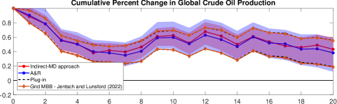
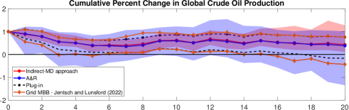
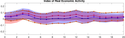
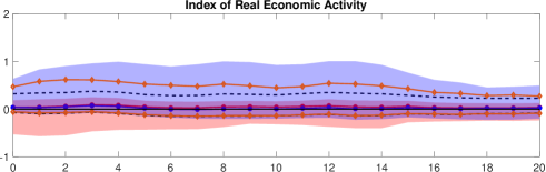
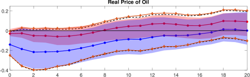
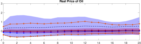
Figure 2: Impulse responses to an oil-supply shock. Red dotted lines correspond to the IRFs estimated with our indirect-MD approach; red shaded areas are the corresponding 68% and 95% MBB confidence intervals; blue dotted lines correspond to the Plug-in IRFs obtained pretending that Kilian’s (2008) proxy is a strong instrument for the oil supply shock; black dashed lines are the 68% and 95% Plug-in confidence intervals; blue shaded areas are the corresponding 68% and 95% weak instruments robust confidence intervals; orange dotted lines correspond to the 68% and 95% “Grid MBB” weak instruments robust confidence intervals.

The blue lines plotted in Figure 2 are the estimated dynamic responses to the oil supply shock identified by Kilian’s (2008) proxy $z_{t}$. More precisely, the graph quantifies the responses of the variables in $Y_{t}:=(prod_{t},rpo_{t},rea_{t})^{\prime}$ to an oil supply shock that increases oil production of 1% on-impact (the responses plotted for $prod_{t}$ are cumulative percent changes). The blue shaded areas depict the corresponding 68% (in panel A) and 95% (in panel B) Anderson-Rubin weak-instrument robust confidence intervals. They closely resemble the IRFs plotted in panels A and B of Figure 1 in Montiel Olea et al. (2021). The orange dotted lines represent Jentsch and Lunsford’s (2021) 68% (in panel A) and 95% (in panel B) ‘grid MBB AR’ confidence intervals. It is evident that the use of the MBB enhances the precision of weak-instrument robust inference on the dynamic causal effects induced by the oil supply shock.

We now move to our indirect-MD approach, which requires instrumenting the non-target shocks $\varepsilon_{2,t}=(\varepsilon_{t}^{AD},\varepsilon_{t}^{OSD})^{\prime}$. The counterpart of system (13) is given by the equation:

$$A_{1\bullet}u_{t}=\alpha_{1,1}u_{t}^{prod}+(\alpha_{1,2},\alpha_{1,3})\left(\begin{array}[]{c}u_{t}^{rea}\\ u_{t}^{rpo}\end{array}\right)=\varepsilon_{t}^{S}$$ (28)

where $A_{1\bullet}=(\alpha_{1,1},$ $\alpha_{1,2},$ $\alpha_{1,3})$. Equation (28) provides the moment condition $A_{1\bullet}\Sigma_{u}A_{1\bullet}^{\prime}=1$, see (14). If, as in Assumption 4, there exist at least $s=n-k=2$ proxies $w_{t}$ for the two non-target shocks $\varepsilon_{2,t}=(\varepsilon_{t}^{AD},\varepsilon_{t}^{OSD})^{\prime}\equiv\tilde{\varepsilon}_{2,t}$, there are two additional moment conditions of the form (15) that can be exploited for inference, i.e. $A_{1\bullet}\Sigma_{u,w}=0_{1\times 2}$, where $\Sigma_{u,w}:=$${E}$$(u_{t}w_{t}^{\prime})$. Overall, there are three moment conditions ($m=\frac{1}{2}k(k+1)+ks=3$) that can be used to estimate the three structural parameters in $A_{1\bullet}$ ($a=3$) by the method discussed in Section 5.

Following the arguments in Kilian (2009) and Montiel Olea et al. (2021), our Assumption 1 is considered valid. Assumption 2 is investigated by a set of diagnostic tests on the VAR residuals (the VAR is estimated with $l=24$ lags), which suggest that the residuals are conditionally heteroskedastic but serially uncorrelated. Assumption 3 is maintained. The validity of the proxies in the sense of Assumption 4 is discussed below.

The proxies selected for the two non-target shocks are $w_{t}:=(w_{t}^{RV},w_{t}^{Br})^{\prime}$, where $w_{t}^{RV}$ represents the logarithmic difference of the World Steel Index (WSI) introduced by Ravazzolo and Vespignani (2020), and $w_{t}^{Br}$ represents the logarithmic difference of the Brent Oil Futures. The proxy $w_{t}^{RV}$ serves as an instrument for the aggregate demand shock, $\varepsilon_{t}^{AD}$, and the proxy $w_{t}^{Br}$ is used as an instrument for the oil-specific demand shock, $\varepsilon_{t}^{OSD}$. Since $w_{t}^{RV}$ is available on the shorter sample, 1990:M2-2004:M9, we employ the entire sample period 1973:M1-2004:M9 to estimate $\Sigma_{u}$ and the shorter sample period, 1990:M2-2004:M9 ($T=176$ monthly observations), to estimate $\Sigma_{u,w}$. Then, the MD estimates of the structural parameters in equation (28) follow from (17)-(18).

We pre-test the strength of the proxies $w_{t}$ by our bootstrap test. In this case, to estimate the parameters that capture the strength of the proxies, $\hat{\theta}_{T}^{\ast}=(\hat{\beta}_{2,T}^{\ast\prime},\hat{\lambda}_{T}^{\ast})^{\prime}$, we consider the sample common to both instruments in $w_{t}$, 1990:M2-2004:M9. We apply the multivariate normality test $\tau_{T,N}^{\ast}\equiv DH$ to the sequence of bootstrap replications $\{\hat{\vartheta}_{T:1}^{\ast},$ $\hat{\vartheta}_{T:2}^{\ast},\ldots,\hat{\vartheta}_{T:N}^{\ast}\}$, where $N=[T^{1/2}]=13$ and $\hat{\vartheta}_{T}^{\ast}\equiv\hat{\theta}_{T}^{\ast}$, with $\hat{\theta}_{T}^{\ast}$ $=(\hat{\beta}_{2,T}^{\ast\prime},\hat{\lambda}_{T}^{\ast})^{\prime}$ being the MBB-CMD estimator discussed in Section 5. The corresponding p-value is 0.67 which does not reject the null hypothesis. As robustness check, we repeat the test using $\hat{\vartheta}_{T}^{\ast}\equiv\hat{\beta}_{2,T}^{\ast\prime}$, obtaining a p-value equal to 0.73. We conclude that the null hypothesis that the proxies $w_{t}:=(w_{t}^{RV},w_{t}^{Br})^{\prime}$ are relevant for the shocks $\tilde{\varepsilon}_{2,t}=(\varepsilon_{t}^{AD},\varepsilon_{t}^{OSD})^{\prime}$ in the sense of condition (11) is not rejected by the data. An indirect check of the exogeneity condition is discussed at the end of this section.

The IRFs estimated by the indirect-MD approach correspond to the red lines plotted in Figure 2. They are surrounded by the red shaded areas representing the 68%-MBB (panel A) and 95%-MBB (panel B) pointwise confidence intervals, computed by using Hall’s percentile method. Proposition 7 ensures that no Bonferroni-type adjustment is needed; see Section 6.4.

From Figure 2, we derive two important observations. First, the MBB confidence intervals obtained by the indirect-MD approach using the strong proxies $w_{t}$ for the non-target shocks – estimated on a shorter sample – are ‘more informative’ than both the Anderson-Rubin weak-instrument robust confidence intervals and the grid MBB AR confidence intervals obtained by instrumenting the oil supply shock directly with Kilian’s (2008) proxy $z_{t}$. Differences become marked when considering $95\%$ confidence intervals, see panel B. Second, our empirical results line up with Kilian’s (2009) main results. In Kilian’s (2009) Choleski-SVAR, both real economic activity and the real price of oil exhibit limited, temporary, and statistically insignificant responses to the oil supply shock. This finding is also evident from our estimated IRFs. Kilian’s (2009) recursive SVAR implies the testable restrictions $A_{1,2}\equiv(\alpha_{1,2}$, $\alpha_{1,3})=(0,0)$ in the structural equation (28). These restrictions imply a vertical short run oil supply curve. Under the conditions outlined in Proposition 2 and with the support of our pre-test that does not reject the relevance of the instruments, a standard Wald-type test conducted on these restrictions produces a bootstrap p-value of 0.68. This evidence aligns with Kilian’s (2009) recursive SVAR. Importantly, according to Proposition 7, the outcome of the Wald test remains unaffected by the failure of the bootstrap pre-test to reject the null hypothesis. As a result, there is no need for Bonferroni adjustments.

To assess the exogeneity (orthogonality) of the proxies $w_{t}$ with respect to the oil supply shock $\varepsilon_{t}^{S}$, we adopt a commonly employed approach in the empirical proxy-SVAR literature. Examples include, e.g., Caldara and Kamps (2017) and Piffer and Podstawki (2018). This involves approximating the shocks of interest by proxies or shocks derived from other studies, or identification methods. In our framework, a natural solution is to calculate the correlations between the proxies $w_{t}$ and Kilian’s (2008) instrument $z_{t}$. We obtain the correlations $\widehat{Corr}(w_{t},z_{t})=(0.0047,$ $-0.09)^{\prime}$ on the common sample 1990:M2-2004:M9, which are not statistically significant at any conventional significance level. An alternative method to assess the exogeneity condition is as follows. The empirical results discussed in this section support Kilian’s (2009) original triangular SVAR specification on the sample 1990:M2-2004:M9, featuring a vertical short run oil supply curve. Other studies suggest, using different identification schemes, that a Choleski-SVAR for $Y_{t}:=(prod_{t},rea_{t},rpo_{t})^{\prime}$ represents a good approximation of the data also on periods longer than the estimation sample 1990:M2-2004:M9; see, e.g., Kilian and Murphy (2012). This suggests that we can interpret the time series $\hat{\varepsilon}_{t}^{S,Chol}$, $t=1,\ldots,T$, recovered from the first equation of Kilian’s (2009) Choleski-SVAR, as a reasonable approximation of an oil supply shock. Also in this case, the correlations computed on the common period 1990:M2-2004:M9, equal to $\widehat{Corr}(w_{t},\hat{\varepsilon}_{t}^{S,Chol})=(-0.059,$ $0.038)^{\prime}$, are not statistically significant at any conventional significance level.

7.2 Financial and macroeconomic uncertainty shocks

In this second empirical illustration, we emphasize the merit of the indirect-MD approach in situations where finding valid multiple instruments for multiple target shocks can be problematic.

Our objective is to track the dynamic causal effects produced by financial and macroeconomic uncertainty shocks ($k=2$) on a measure of the real economic activity. As in Ludvigson et al. (2021), we consider a small-scale VAR model with $n=3$ variables: $Y_{t}:=(U_{F,t},U_{M,t},a_{t})^{\prime}$, where $U_{F,t}$ is an index of (1-month ahead) financial uncertainty, $U_{M,t}$ is the index of (1-month ahead) macroeconomic uncertainty, and $a_{t}$ is a measure of real economic activity, proxied by the growth rate of industrial production. The two uncertainty indexes are analyzed and discussed in Ludvigson et al. (2021), where the authors contend that unraveling the relative impacts of these two distinct sources of uncertainty is crucial for understanding how they are transmitted to the business cycle.

We focus on the ‘Great Recession + Slow Recovery’ period 2008:M1-2015:M4 ($T=88$ monthly observations). The dataset is the same as in Ludvigson et al. (2021) and Angelini et al. (2019). The decision to focus on the period following the Global Financial Crisis is based on the empirical findings presented in Angelini et al. (2019), where it was discovered that the VAR model for $Y_{t}:=(U_{F,t},U_{M,t},a_{t})^{\prime}$ exhibits two significant breaks in unconditional volatility over the extended period from 1960 to 2015, resulting in three distinct volatility regimes.

The reduced form VAR model for $Y_{t}$ includes a constant and $l=4$ lags. The VAR residuals display neither serial correlation, nor conditionally heteroskedasticity on the sample 2008:M1-2015:M4.

The target structural shocks are collected in the vector $\varepsilon_{1,t}:=(\varepsilon_{F,t},\varepsilon_{M,t})^{\prime}$, where $\varepsilon_{F,t}$ denotes the financial uncertainty shock and $\varepsilon_{M,t}$ the macroeconomic uncertainty shock. The non-target shock of the system is the ‘non-uncertainty’ shock $\varepsilon_{a,t}\equiv\tilde{\varepsilon}_{2,t}$ $(n-k=1)$, which can be interpreted as a shock reflecting forces related to real economic activity. In this model, the counterpart of (4) is as follows:

$$\underset{u_{t}}{\underbrace{\left(\begin{array}[]{c}u_{F,t}\\ u_{M,t}\\ u_{a,t}\end{array}\right)}}=\underset{B_{\bullet 1}}{\underbrace{\left(\begin{array}[]{cc}\beta_{F,F}&\beta_{F,M}\\ \beta_{M,F}&\beta_{M,M}\\ \beta_{a,F}&\beta_{a,B}\end{array}\right)}}\underset{\varepsilon_{1,t}}{\underbrace{\left(\begin{array}[]{c}\varepsilon_{F,t}\\ \varepsilon_{M,t}\end{array}\right)}}+\underset{B_{\bullet 2}}{\underbrace{\left(\begin{array}[]{c}b_{F,a}\\ b_{M,a}\\ b_{a,a}\end{array}\right)}}\underset{\varepsilon_{2,t}}{\underbrace{\left(\varepsilon_{a,t}\right)}}$$ (29)

where $u_{t}:=(u_{F,t},u_{M,t},u_{a,t})^{\prime}$ is the vector of VAR reduced form disturbances. The implementation of the direct identification approach presents a challenge in identifying two reliable external instruments for the two uncertainty shocks $\varepsilon_{1,t}:=(\varepsilon_{F,t},\varepsilon_{M,t})^{\prime}$. Ludvigson et al. (2021, p. 6) acknowledge that in this application ‘Instrumental variable analysis is challenging, since instruments that are credibly exogenous are difficult if not impossible to find…’.

We show that the indirect-MD approach simplifies the process of inferring the effects of macroeconomic and financial uncertainty shocks on real economic activity. Indeed, the indirect approach enables us to shift the issue of identifying (at least) two valid proxies for the two uncertainty shocks to the task of finding (at least) one valid instrument for the shock in real economic activity. This requires considering the equations

$$A_{1\bullet}u_{t}\equiv\underset{A_{1,1}}{\underbrace{\left(\begin{array}[]{cc}\alpha_{F,F}&\alpha_{F,M}\\ \alpha_{M,F}&\alpha_{M,M}\end{array}\right)}}\underset{u_{1,t}}{\underbrace{\left(\begin{array}[]{c}u_{F,t}\\ u_{M,t}\end{array}\right)}}+\underset{A_{1,2}}{\underbrace{\left(\begin{array}[]{c}\alpha_{F,a}\\ \alpha_{M,a}\end{array}\right)}}\underset{u_{2,t}}{\underbrace{\left(u_{a,t}\right)}}\text{ }=\text{ }\varepsilon_{1,t}\equiv\left(\begin{array}[]{c}\varepsilon_{F,t}\\ \varepsilon_{M,t}\end{array}\right)$$ (30)

which represents the counterpart of system (13). Since $k=2$, point-identification of the target uncertainty shocks requires at least $\frac{1}{2}k(k-1)=1$ extra restriction on the elements of the matrix $A_{1\bullet}$. Equation (30) provides $\frac{1}{2}k(k+1)=3$ moment conditions implied by the expression $A_{1\bullet}^{\prime}\Sigma_{u}A_{1\bullet}=I_{2}$. As $n-k=1$, we need at least one external instrument for the non-target shock; i.e., a variable $w_{t}$ ($s=n-k=1$) that satisfies the linear measurement equation

$$w_{t}=\lambda\varepsilon_{a,t}+\omega_{w,t}$$ (31)

where $\tilde{\varepsilon}_{2,t}=\varepsilon_{a,t}$, $\lambda$ is the relevance parameter and $\omega_{w,t}$ is a measurement error term, uncorrelated with structural shocks. Equation (31) is the counterpart of (10) in Assumption 4 and provides two additional moment restrictions, $A_{1\bullet}^{\prime}\Sigma_{u,w}=0_{2\times 1}$, where $\Sigma_{u,w}:=$${E}$$(u_{t}w_{t})$. By jointly considering the restrictions $A_{1\bullet}^{\prime}\Sigma_{u}A_{1\bullet}=I_{2}$ and $A_{1\bullet}^{\prime}\Sigma_{u,w}=0_{2\times 1}$, we obtain a total of $m=3+2=5$ distinct and independent moment conditions which can be used to estimate $a=5$ structural parameters in $A_{1\bullet}$. To impose the necessary identification constraint on $A_{1\bullet}$, we borrow the restriction$\ \beta_{F,M}=0$ (on $B_{\bullet 1}$) from Angelini et al. (2019). Using a methodology based on changes in volatility regimes and considering the extended period 1960-2015, Angelini et al. (2019) explore the idea that instantaneous causality between uncertainty shocks solely runs from financial to macroeconomic uncertainty. They test the hypothesis that financial uncertainty does not respond instantaneously to macroeconomic uncertainty shocks ($\beta_{F,M}=0$) and do not reject this hypothesis for the sample period 2008:M1-2015:M4. By using the relationship (2), the restriction $\beta_{F,M}=e_{3,1}^{\prime}(B_{\bullet 1})e_{2,2}=0$ (recall that, e.g., $e_{3,1}$ is the $3\times 1$ vector containing ‘1’ in the position $1$ and zero elsewhere$)$ can be mapped to the elements of $A_{1\bullet}^{\prime}$ via $e_{3,1}^{\prime}(\Sigma_{u}A_{1\bullet}^{\prime})e_{2,2}=0$, and properly expressed in the form (16) once $\Sigma_{u}$ is replaced by its consistent estimator $\hat{\Sigma}_{u}:=T^{-1}\sum_{t=1}^{T}\hat{u}_{t}\hat{u}_{t}^{\prime}$. This allows to estimate $a=5$ free structural parameters in the matrix $A_{1\bullet}$ by or MD approach. On the other hand, the constraint $\beta_{F,M}=0$ can be directly incorporated in the estimation of the proxy-SVAR by relying on the alternative indirect-MD estimation method discussed in the Supplement, Section S.5.

To find a valid proxy $w_{t}$ for the real economic activity shock $\varepsilon_{a,t}$, we follow Angelini and Fanelli (2019). Let $house_{t}$ be the log of new privately owned housing units started on the estimation period 2008:M1-2015:M4 (source: Fred). We take the ‘raw’ growth rate of new privately owned housing units started, $\Delta house_{t}$, and estimate an auxiliary dynamic linear regression model of the form $\Delta house_{t}=$${E}$$(\Delta house_{t}\mid\mathcal{F}_{t-1})+err_{t}$, where $\mathcal{F}_{t-1}$ denotes the information set available to the econometrician at time $t-1$, ${E}$$(\Delta house_{t}\mid\mathcal{F}_{t-1})$ denotes the linear projection of $\Delta house_{t}$ on the past information set, and $err_{t}$ can be interpreted as the ‘innovation component’ of the dynamic auxiliary model for the external instrument. The residuals, denoted as $w_{t}:=$ $\widehat{err}_{t}$, $t=1,\ldots,T$, resulting from regressing $\Delta house_{t}$ on past information, serve as our approximation for the shock in real economic activity.

We pre-test the strength of the proxy $w_{t}$ by computing our bootstrap test of instrument relevance. We apply the DH multivariate normality test to the bootstrap replications $\{\hat{\vartheta}_{T:1}^{\ast},\hat{\vartheta}_{T:2}^{\ast},\ldots,\hat{\vartheta}_{T:N}^{\ast}\}$, where $\hat{\vartheta}_{T:b}^{\ast}\equiv\hat{\beta}_{2,T:b}^{\ast}$, $b=1,\ldots,N$, $N=[T^{1/2}]=9$, and $\hat{\theta}_{T}^{\ast}=(\hat{\beta}_{2,T}^{\ast\prime},\hat{\lambda}_{T}^{\ast})^{\prime}\$is the MBB-CMD estimator discussed in Section 5. The DH multivariate normality test yields a p-value of 0.38, indicating no rejection of the null hypothesis of relevant proxy.

To indirectly assess the exogeneity condition, we examine the correlation between our proxy variable $w_{t}$ and time series data of macroeconomic and financial uncertainty shocks, as determined by Angelini et al. (2019) using their approach based on changes in unconditional volatility. Specifically, we consider their estimated time series $\hat{\varepsilon}_{F,t}$ and $\hat{\varepsilon}_{M,t}$, $t=1,\ldots,T$. The resulting correlations, computed over the sample period 2008:M1-2015:M4, are $\widehat{Corr}(w_{t},(\hat{\varepsilon}_{F,t},\hat{\varepsilon}_{M,t})^{\prime})=(-0.092,$ $-0.096)^{\prime}$ and are not statistically significant at any conventional level.

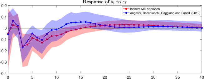
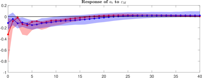
Figure 3: Impulse responses of industrial production growth ($a_{t}$) to a one standard deviation financial ($\varepsilon_{F}$) and a macro ($\varepsilon_{M}$) uncertainty shocks. Red dotted lines correspond to the IRFs estimated with our indirect-MD approach; red shaded areas are the corresponding 90% MBB confidence intervals; blue dotted lines correspond to the IRFs obtained by Angelini et at. (2019); blue shaded areas correspond to their 90% (iid, bootstrap) confidence intervals.

After estimating the model using the indirect-MD approach, we generate IRFs for a 40-month period. In Figure 3, the red lines (labelled as ‘indirect-MD approach’) represent the dynamic responses of the growth rate of industrial production to identified financial (upper panel) and macroeconomic (lower panel) uncertainty shocks. These responses are based on one-standard deviation uncertainty shocks and are surrounded by 90% MBB confidence intervals (depicted as red shaded areas), calculated using Hall’s percentile method. According to Proposition 7, the asymptotic coverage of these confidence intervals remains unaffected by pre-testing bias. To allow for easy comparison with a benchmark, Figure 3 also incorporates the responses obtained by Angelini et al. (2019), shown in blue and identified as ‘Angelini, Bacchiocchi, Caggiano, and Fanelli (2019)’ (refer to their Figure 5). These responses are also based on one-standard deviation uncertainty shocks. The blue shaded region in Figure 3 represents the 90% bootstrap confidence intervals computed by Angelini et al. (2019) over the period 2008:M1-2015:M4, using the i.i.d. bootstrap method.

Figure 3 unveils two important findings. First, both the indirect-MD approach and Angelini et al.’s (2019) method reveal a significant effect of macroeconomic and financial uncertainty shocks in restraining economic activity during the post-Great Recession period. Secondly, substantial disparities emerge in the estimated impact of the macroeconomic uncertainty shock on industrial production growth. Using the indirect-MD approach, the estimated peak response of industrial production growth to the macroeconomic uncertainty shock is both significant and instantaneous, equal to -0.32%. Conversely, the method based on changes in volatility indicates that the peak response, also statistically significant, occurs five months post-shock, with a magnitude of -0.15%. In both the indirect-MD approach and the volatility-based approach, the peak response of industrial production growth to the financial uncertainty shock is significant, equal to -0.17%. Upon examination of the 90% bootstrap confidence intervals, it becomes evident that the dynamic causal effects resulting from macroeconomic and financial uncertainty shocks are more precisely estimated through the indirect-MD approach.

8 Conclusions

We have designed a MD estimation strategy for proxy-SVARs in which strong proxies for the non-target shocks are used to identify the target shocks. This approach proves particularly effective when the instruments available for the target shocks are weak. It becomes especially advantageous when, faced with multiple target shocks, the application of weak-instrument robust methods necessitates imposing a large number of restrictions which might lack economic motivation and/or could pose challenges in terms of testing their validity. Furthermore, we have enriched this proposed strategy with a novel, computationally straightforward diagnostic pre-test for instrument relevance which relies on bootstrap resampling and does not introduce any pre-testing bias.

It could be argued that in models of the dimensions typically encountered in practice, obtaining valid proxies for the non-target shocks and establishing additional credible identifying restrictions that are sufficient to uniquely point-identify the target structural shocks can be challenging. However, the empirical illustrations revisited in this paper demonstrate the potential benefits and effectiveness of the suggested approach in cases of interest. One question that arises is whether it is appropriate to solely instrument the non-target shocks without considering any information from available weak proxies for the target shocks, as this approach may overlook potentially valuable identifying information. In principle, one may use both proxies for the non-target shocks and proxies for the target shocks jointly. Intuitively, in such situations, the strong proxies for the non-target shocks act as a form of ‘insurance’ against potential identification issues that could arise if the proxies for the target shocks were weak, allowing for more reliable inference. Exploring this intriguing issue further will be the focus of our future research.

Acknowledgements

We thank Luca Gambetti, Iliyan Georgiev, Alexander Kriwoluzky, Lutz Kilian, Daniel Lewis, Helmut Lütkepohl, Sophocles Mavroeidis, Mikkel Plagborg-Møller, Ben Schumann, Lorenzo Trapani, as well as seminar participants at the SIdE Webinar Series (March 2021), the Granger Centre for Time Series Econometrics at the University of Nottingham (March 2022), and participants to the Workshop ‘Advances in Structural Shocks Identification: Information, Fundamentalness and Recoverability’ (Barcelona GSE Summer Forum, June 2021), the IAAE 2021 Annual Meeting (Rotterdam, June 2021), the EEA-ESEM 2021 (Virtual, August 2021), the DIW Berlin ‘Macroeconometric Workshop’ (Berlin, May 2022). We gratefully acknowledge financial support from MIUR (PRIN 2017, Grant 2017TA7TYC) and the University of Bologna (RFO grants).

References

Anderson, T.W. and Rubin, H. (1949), Estimation of the parameters of a single equation in a complete system of stochastic equations, Annals of Mathematical Statistics 20, 46-63.

Andrews, D.W. K. and Cheng, X. (2012) Estimation and inference with weak, semi-strong, and strong identification, Econometrica 80, 2153-2211.

Andrews, I., Stock, J.H. and Sun, L. (2019), Weak instruments in instrumental variables regression: Theory and practice, Annual Review of Economics 11, 727-753.

Angelini, G. and Fanelli, L. (2019), Exogenous uncertainty and the identification of Structural Vector Autoregressions with external instruments, Journal of Applied Econometrics 34, 951-971.

Angelini, G., Bacchiocchi, E., Caggiano, G., and Fanelli, L. (2019), Uncertainty across volatility regimes, Journal of Applied Econometrics 34, 437-455.

Angelini, G., Cavaliere, G. and Fanelli, L. (2022), Bootstrap inference and diagnostics in state space models: with applications to dynamic macro models, Journal of Applied Econometrics 37, 3-22.

Arias, J.E., Rubio-Ramirez, J.F. and Waggoner, D.F. (2021), Inference in Bayesian Proxy-SVARs, Journal of Econometrics 225, 88-106.

Bacchiocchi, E. and Kitagawa, T. (2022), Locally- but not globally-identified SVARs, Quaderni - Working Paper DSE n. 1171, 2022, available at SSRN: https://ssrn.com/abstract=4124228 or http://dx.doi.org/10.2139/ssrn.4124228.

Bose, A. (1988), Edgeworth correction by bootstrap in Autoregressions, Annals of Statistics 16, 1709-1722.

Boubacar Mainnasara, Y. and Francq, C. (2011), Estimating structural VARMA models with uncorrelated but non-independent error terms, Journal of Multivariate Analysis 102, 496-505.

Brüggemann, R., Jentsch, C. and Trenkler, C. (2016), Inference in VARs with conditional volatility of unknown form, Journal of Econometrics 191, 69-85.

Caldara, D. and Herbst, E. (2019), Monetary policy, real activity, and credit spreads: Evidence from Bayesian Proxy SVARs, American Economic Journal: Macroeconomics 11, 157-92.

Caldara, D. and Kamps, C. (2017), The analytics of SVARs: A unified framework to measure fiscal multipliers, Review of Economic Studies 84, 1015-1040.

Cavaliere, G. and Georgiev, I. (2020), Inference under random limit bootstrap measures, Econometrica 88, 2547-2974.

Francq, C. and Raïssi, H. (2006), Multivariate portmanteau test for autoregressive models with uncorrelated but nonindependent errors, Journal of Time Series Analysis 28, 454-470.

Giacomini, R., Kitagawa, T. and Read, M. (2022), Robust Bayesian inference in Proxy SVARs, Journal of Econometrics 228, 107-126.

Hahn, J. and Hausman, J. (2002), A new specification test for the validity of instrumental variables, Econometrica 70, 163-189.

Hall, P. (1992), The bootstrap and Edgeworth expansion, Springer-Verlag, Berlin.

Hausman, J., Stock, J.H. and Yogo, M. (2005), Asymptotic properties of the Hahn-Hausman test for weak instruments, Economic Letters 89, 333-342.

Horowitz, J.L. (2001), The bootstrap, Handbook of Econometrics Vol. 5, Heckman, J.J. and E. Leamer (eds.), Ch. 52.

Jentsch, C. and Lunsford, K.C. (2019), The dynamic effects of personal and corporate income tax changes in the United States: Comment, American Economic Review 109, 2655-2678.

Jentsch, C. and Lunsford, K.C. (2022), Asymptotic valid bootstrap inference for Proxy SVARs, Journal of Business and Economic Statistics 40, 1876–1891. 

Kilian, L. (1998), Small-sample confidence intervals for impulse response functions, Review of Economics and Statistics 80, 218-230.

Kilian, L. (2008), Exogenous oil supply shocks: How big are they and how much do they matter for the U.S. economy? Review of Economics and Statistics 90, 216-240.

Kilian, L. (2009), Not all oil shocks are alike: Disentangling demand and supply shocks in the crude oil market, American Economic Review 99, 1053-1069.

Kilian, L. and Murphy, D. P. (2012), Why agnostic sign restrictions are not enough: Understanding the dynamics of oil market VAR models, Journal of the European Economic Association 10, 1166-1188.

Leeper, E.M, Sims, C.A. and Zha, T. (1996), What does monetary policy do? Brooking Papers of Economic Activity 27, 1-78.

Lilliefors, H. (1967), On the Kolmogorov-Smirnov test for normality with mean and variance unknown, Journal of the American Statistical Association 62, 399-402.

Ludvigson, S.C., Ma, S. and Ng, S. (2021), Uncertainty and business cycles: exogenous impulse or endogenous response? American Economic Journal: Macroeconomics 13, 369-410.

Lunsford, K. G. (2016), Identifying Structural VARs with a proxy variable and a test for a weak proxy, Federal Reserve Bank of Cleveland Working Paper no. 15-28 (version dated October 2016).

Mertens, K. and Ravn, M. (2013), The dynamic effects of personal and corporate income tax changes in the United States, American Economic Review 103, 1212-1247.

Mertens, K. and Ravn, M. (2019), The dynamic effects of personal and corporate income tax  changes in the United States: Reply to Jentsch and Lunsford, American Economic Review 109, 2679-2691.

Montiel Olea, J.L. and Pflueger, C. (2013), A robust test for weak instruments, Journal of Business and Economic Statistics 31, 358-369.

Montiel Olea, J.L., Stock, J.H. and Watson, M.W. (2021), Inference in SVARs identified with an external instrument, Journal of Econometrics 225, 74-87.

Newey, W.K. and McFadden, D. (1994), Large sample estimation and hypothesis testing, Handbook of Econometrics, R.F. Engle and D.L. McFadden (eds.), Vol. IV, Chap. 36.

Piffer, M. and Podstawki, M. (2018), Identifying uncertainty shocks using the price of gold, The Economic Journal, 128, 3266-3284.

Ravazzolo, F., Vespignani, J. (2020), World steel production: A new monthly indicator of global real economic activity, Canadian Journal of Economics 53, 743-766.

Staiger, D. and Stock, J. H. (1997), Instrumental variables regressions with weak instruments, Econometrica 65, 557-586.

Stock, J.H. (2008), What’s New in Econometrics-Time Series, Lecture 7. Structural VARs, Cambridge, MA., NBER.

Stock, J.H. and Watson, M.W. (2012), Disentangling the channels of the 2007–2009 recession, in Brookings Panel of Economic Activity, Spring 2012, 81-135.

Stock J.H. and Yogo, M. (2005), Testing for weak instruments in linear IV regression. In Identification and Inference for Econometric Models: Essays in Honor of Thomas Rothenberg, ed. D.W.K. Andrews, J.H. Stock, 80–108. Cambridge, UK: Cambridge University Press.

Stock J.H. and Wright, J. (2000), GMM with weak identification, Econometrica 68, 1055–96.

Zivot, E., Startz, R. and Nelson, C.R. (1998), Valid confidence regions and inference in the presence of weak instruments, International Economic Review 39, 1119-1146.

Rejection frequencies
Strong proxy
	$T=250$		$T=1000$
	$corr=0.59$		$corr=0.59$
${\theta}$	${DH}$	${KS}$	${DH}$	${KS}$
$\beta_{2,1}$	0.05(0.06)	0.05(0.06)	0.05(0.05)	0.05(0.05)
$\beta_{2,2}$		0.05(0.06)		0.05(0.05)
$\beta_{2,3}$		0.05(0.05)		0.05(0.05)
$\lambda$		0.05(0.05)		0.05(0.05)
Moderately weak proxy
	$T=250$		$T=1000$
	$corr=0.25$		$corr=0.13$
${\theta}$	${DH}$	${KS}$	${DH}$	${KS}$
$\beta_{2,1}$	0.22(0.22)	0.21(0.23)	0.80(0.63)	0.36(0.35)
$\beta_{2,2}$		0.27(0.29)		0.38(0.39)
$\beta_{2,3}$		0.20(0.24)		0.30(0.33)
$\lambda$		0.09(0.09)		0.10(0.12)
Weak proxy
	$T=250$		$T=1000$
	$corr=0.05$		$corr=0.02$
${\theta}$	${DH}$	${KS}$	${DH}$	${KS}$
$\beta_{2,1}$	0.72(0.75)	0.80(0.78)	0.98(0.98)	0.93(0.93)
$\beta_{2,2}$		0.85(0.83)		0.95(0.95)
$\beta_{2,3}$		0.82(0.83)		0.95(0.95)
$\lambda$		0.24(0.26)		0.50(0.51)

Table 1: Empirical rejection frequencies of the bootstrap pre-test of instrument relevance.

Notes: Results are based on $20,000$ simulations and tuning parameter $N:=[T^{1/2}]$. $corr=corr(w_{t},\varepsilon_{2,t})$ is the correlation between the instrument $w_{t}$ and the non-target structural shock $\varepsilon_{2,t}$. KS is Lilliefors’ (1967) version of Kolgomorov-Smirnov univariate normality test; $DH$ is Doornik and Hansen’s (2008) multivariate normality test. Results (not) in parenthesis refer to (iid) GARCH-type VAR disturbances and proxies. The block size in the MBB algorithm is $l=5.03T^{1/4}$, see footnote 18. All tests are computed at the 5% nominal significance level.

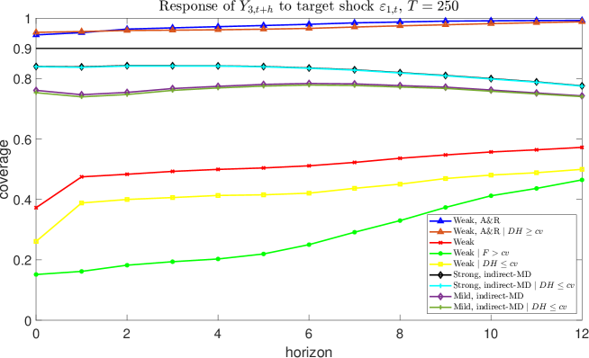
Figure 1: Empirical coverage probabilities of IRFs calculated on $20,000$ simulations (90% nominal). IRFs refer to the response of the variable $Y_{3,t+h}$ to the target shock $\varepsilon_{1,t}$, $h=0,1,...,12$.

A. 68% confidence intervals		B. 95% confidence intervals

SUPPLEMENT TO:

‘AN IDENTIFICATION AND TESTING STRATEGY FOR PROXY-SVARS WITH WEAK PROXIES’

By Giovanni Angelini, Giuseppe Cavaliere, Luca Fanelli

First draft: September 2021. First revision: September 2022. 

Second revision: July 2023.  This version: October 2023

Appendix S.1 Introduction

This supplement complements the results of the paper along several dimensions. Section S.2 summarizes the notation used for the bootstrap as well as some additional matrix notation. Section S.3 presents the auxiliary lemmas used to prove the main propositions in the paper, and Section S.4 contains the proofs of lemmas and propositions.

Section S.5 revisits the indirect-MD approach discussed in Section 5, using a different parameterization of the proxy-SVAR. Section S.6 compares the MD estimation method with the IV approach. Section S.7 sketches the MBB algorithm mentioned in the paper and used to build our test of instrument relevance. Section S.8 provides details on the DGPs used in the Monte Carlo experiments in Section 6.3 of the paper. Finally, Section S.9 provides an additional empirical illustration, where a fiscal proxy-SVAR is used to infer US fiscal multipliers on quarterly data.

Unless differently specified, all references – except those starting with ‘S.’ – pertain to sections, assumptions, equations, and results in the main paper.

Appendix S.2 Notation

Bootstrap. We use $P$ to denote the probability measure for the data, and ${E}(\cdot)$ and ${Var}(\cdot)$ to denote expectations and variance computed under $P$, respectively. We use $P^{\ast}$ to denote the probability measure induced by the bootstrap; i.e., conditional on the original sample. Expectation and variance computed under $P^{\ast}$ are denoted by ${E}^{\ast}(\cdot)$ and ${Var}^{\ast}(\cdot)$, respectively.

Let, for any $\varsigma>0$, $p_{T}^{\ast}(\varsigma):=P^{\ast}(||\hat{\theta}_{T}^{\ast}-\hat{\theta}_{T}||>\varsigma)$, where $\hat{\theta}_{T}^{\ast}$ is the bootstrap analog of the estimator $\hat{\theta}_{T}$, and let $\left\|\cdot\right\|$ denote the Euclidean norm. With the notation ‘$\hat{\theta}_{T}^{\ast}-\hat{\theta}_{T}\overset{p^{\ast}}{\rightarrow}_{p}0$’, which reads ‘$\hat{\theta}_{T}^{\ast}-\hat{\theta}_{T}$ converges in $P^{\ast}$ to $0$, in probability’, we mean that the (stochastic) sequence $\left\{p_{T}^{\ast}(\varsigma)\right\}$ converges in probability to zero ($p_{T}^{\ast}(\varsigma)\overset{p}{\rightarrow}0$).

Consider a scalar a random variable $X$, with associated cdf $\digamma_{X}(x):=P(X\leq x)$, and a bootstrap sequence $\{X_{T}^{\ast}\}$, where $X_{T}^{\ast}$ has associated cdf (conditional on the data) $\digamma_{X_{T}^{\ast}}^{\ast}(x):=P^{\ast}(X_{T}^{\ast}\leq x)$. We say that $X_{T}^{\ast}$ ‘converges in conditional distribution to $X$, in probability’, denoted ‘$X_{T}^{\ast}\overset{d^{\ast}}{\rightarrow}_{p}X$’, if $\digamma_{X_{T}^{\ast}}^{\ast}(x)\overset{p}{\rightarrow}\digamma_{T}(x)$ for each $x$ at which $\digamma_{X}(x)$ is continuos. Notice that if $\digamma_{X}(\cdot)$ is continuous, then the latter convergence also implies that $\sup_{x\in\mathbb{R}}|\digamma_{X_{T}^{\ast}}^{\ast}(x)-\digamma_{X}(x)|\overset{p}{\rightarrow}0$ by Pólya’s theorem. These definitions can be extended to the multivariate framework in the conventional way.

Matrices. In the results and proofs that follow we refer the following matrices (Magnus and Neudecker, 1999): $D_{n}$ is the $n$-dimensional duplication matrix ($D_{n}{vech}(M)={vec}(M)$, $M$ being an $n\times n$ matrix) and $D_{n}^{+}:=(D_{n}^{\prime}D_{n})^{-1}D_{n}$ is the Moore-Penrose generalized inverse of $D_{n}$; $K_{ns}$ is the $ns$-dimensional commutation matrix ($K_{ns}{vec}(M)={vec}(M^{\prime})$, $M$ being $n\times s$).

Appendix S.3 Auxiliary lemmas

This section summarizes the lemmas useful for the propositions considered in the paper. We initially represent the proxy-SVAR in a form that facilitates the derivation of the reduced form parameter estimator.

Estimator of the reduced form parameters. By coupling the VAR for $Y_{t}$ in equation (3) with the proxies available for the non-target shocks $w_{t}$ in equation (10) (see Assumption 4), the proxy-SVAR can be represented as the ‘large’, parametrically constrained, VAR model:

$$\left(\begin{array}[]{cc}I_{n}-\Pi(L)&0\\ 0&I_{s}\end{array}\right)\underset{W_{t}}{\underbrace{\left(\begin{array}[]{c}Y_{t}\\ w_{t}\end{array}\right)}}=\underset{\eta_{t}}{\underbrace{\left(\begin{array}[]{c}u_{t}\\ w_{t}\end{array}\right)}}\text{, \ }\Sigma_{\eta}:=\left(\begin{array}[]{cc}\Sigma_{u}&\Sigma_{u,w}\\ \Sigma_{w,u}&\Sigma_{w}\end{array}\right)$$ (S.1)

where $\Pi(L):=\Pi_{1}L+$ $\ldots$ $+\Pi_{l}L^{l}$. In (S.1), the proxies in $w_{t}$ are expressed in innovation form; i.e., they are serially uncorrelated. In applications, however, it may happen that the ‘raw’ observed proxy $w_{t}$ is serially autocorrelated and generated by a dynamic model of the form: $w_{t}={E}_{t-1}w_{t}+\rho_{w,t}$, where ${E}_{t-1}w_{t}$ may depend on variables in the information set a time $t-1$, and $\rho_{w,t}$ is the associated ‘unsystematic component’ innovation; in this case, $\rho_{w,t}$ is assumed to satisfy the same $\alpha$-mixing conditions postulated for the VAR innovations $u_{t}$ in Assumption 2. System (S.1) can be generalized to the representation

$$\left(\begin{array}[]{cc}I_{n}-\Pi(L)&0\\ \Xi_{w,y}(L)&I_{s}-\Xi_{w,w}(L)\end{array}\right)\underset{W_{t}}{\underbrace{\left(\begin{array}[]{c}Y_{t}\\ w_{t}\end{array}\right)}}=\underset{\eta_{t}}{\underbrace{\left(\begin{array}[]{c}u_{t}\\ \rho_{w,t}\end{array}\right)}}\text{, \ }\Sigma_{\eta}:=\left(\begin{array}[]{cc}\Sigma_{u}&\Sigma_{u,w}\\ \Sigma_{w,u}&\Sigma_{w}\end{array}\right)$$ (S.2)

where $\Xi_{w,y}(L)$ and $\Xi_{w,w}(L)$ are matrix polynomials in the lag operator assumed, without loss of generality, of order not larger than $l$ and such that the roots of the characteristic equation $\det(I_{s}-\Xi_{w,w}(x))=0$ satisfy the condition $\left|x\right|>1$. Under Assumption 1, the stability condition on $I_{s}-\Xi_{w,w}(L)$ ensures that system (S.1) remains asymptotically stable. Regardless of whether we consider system (S.1) or (S.2), the proxy-SVAR innovations $\eta_{t}:=(u_{t}^{\prime},w_{t}^{\prime})^{\prime}$ or $\eta_{t}:=(u_{t}^{\prime},\rho_{w,t}^{\prime})^{\prime}$ satisfy the $\alpha$-mixing properties in Assumption 2.

Given $W_{t}:=(Y_{t}^{\prime},w_{t}^{\prime})^{\prime}$ of dimension $(n+s)\times 1$, we compact the proxy-SVAR (either system (S.1) or (S.2)) as

$$W_{t}=\Psi_{1}W_{t-1}+\Psi_{2}W_{t-2}+\ldots+\Psi_{l}W_{t-l}+\eta_{t}\text{ }$$ (S.3)

where each $\Psi_{i}$, $i=1,\ldots,l$, has a triangular structure. Henceforth, we denote with $\delta_{\psi}$ the vector that collects the non-zero autoregressive parameters in the matrices $\Psi_{i}$, $i=1,\ldots,l$, and with $\delta_{\eta}$ the vector that collects the non-repeated elements in the covariance matrix $\Sigma_{\eta}$. Jointly, the reduced form parameters of the proxy-SVAR are in the vector $\delta:=(\delta_{\psi}^{\prime},\delta_{\eta}^{\prime})^{\prime}$ of dimension $q\times 1,$ with $q=q_{\psi}+q_{\eta}$; $q_{\psi}$ is the dimension of $\delta_{\psi}$ and $q_{\eta}$ the dimension of $\delta_{\eta}$. $\delta_{0}:=(\delta_{\psi,0}^{\prime},\delta_{\eta,0}^{\prime})^{\prime}$ is the true value of $\delta$ and $\hat{\delta}_{T}:=(\hat{\delta}_{\psi,T}^{\prime},\hat{\delta}_{\eta,T}^{\prime})^{\prime}$ the quasi-maximum likelihood [QML] estimator. Further, we consider a MBB analog of the QML estimator of $\delta:=(\delta_{\psi}^{\prime},\delta_{\eta}^{\prime})^{\prime}$, denoted $\hat{\delta}_{T}^{\ast}:=(\hat{\delta}_{\psi,T}^{\ast\prime},\hat{\delta}_{\eta,T}^{\ast\prime})^{\prime}$. A sequence of $N$ bootstrap replications of this estimator, $\{\hat{\delta}_{T:1}^{\ast},\ldots\hat{\delta}_{T:N}^{\ast}\}$, can be obtained with the MBB algorithm sketched in Section S.7.

Lemmas. Lemma S.1 deals with the asymptotic properties of the non-bootstrap and bootstrap estimators of the parameters $\delta:=(\delta_{\psi}^{\prime},\delta_{\eta}^{\prime})^{\prime}$. Below, $\ell$ denotes the parameter that governs the block length in MBB resampling, see Jentsch and Lunsford (2019, 2022) and Section S.7.

Lemma S.1

Consider the proxy-SVAR model (S.3). Let $\hat{\delta}_{T}:=(\hat{\delta}_{\psi,T}^{\prime},\hat{\delta}_{\eta,T}^{\prime})^{\prime}$ and $\hat{\delta}_{T}^{\ast}:=(\hat{\delta}_{\psi,T}^{\ast\prime},\hat{\delta}_{\eta,T}^{\ast\prime})^{\prime}$ be as defined above. Under Assumptions 1, 2 and 4, for sequences of models in which ${E}(w_{t}\tilde{\varepsilon}_{2,t}^{\prime})=\Lambda_{T}\rightarrow\Lambda$:
(i)

$$\hat{\delta}_{T}-\delta_{0}\overset{p}{\rightarrow}0_{q\times 1};$$ (S.4)

$$T^{1/2}\left(\begin{array}[]{c}\hat{\delta}_{\psi,T}-\delta_{\psi,0}\\ \hat{\delta}_{\eta,T}-\delta_{\eta,0}\end{array}\right)\overset{d}{\rightarrow}N(0_{q\times 1},V_{\delta})\ ,\ V_{\delta}:=\left(\begin{array}[]{cc}V_{\psi}&V_{\psi,\eta}\\ V_{\psi,\eta}^{\prime}&V_{\eta}\end{array}\right);$$ (S.5)

(ii) under the additional condition $\ell^{3}/T\rightarrow 0$:

$$\hat{\delta}_{T}^{\ast}-\hat{\delta}_{T}\overset{p^{\ast}}{\rightarrow}_{p}0_{q\times 1}$$ (S.6)

$$T^{1/2}V_{\delta}^{-1/2}\left(\begin{array}[]{c}\hat{\delta}_{\psi,T}^{\ast}-\hat{\delta}_{\psi,T}\\ \hat{\delta}_{\eta,T}^{\ast}-\hat{\delta}_{\eta,T}\end{array}\right)\overset{d^{\ast}}{\rightarrow}_{p}N(0_{q\times 1},I_{q}).$$ (S.7)

The results in Lemma S.1 are robust to the strength of the proxies; i.e., they hold regardless of whether the proxies $w_{t}$ satisfy the condition (11) or (12) in Section 4. The structure of the asymptotic covariance matrix $V_{\delta}$ in (S.5) is specified in detail in Brüggemann, Jentsch and Trenkler (2016). It can be proved it has a ‘sandwich’ form $V_{\delta}:=\mathcal{A}_{0}^{-1}\mathcal{B}_{0}\mathcal{A}_{0}^{-1\prime}$, where $\mathcal{A}_{0}:=\lim_{T\rightarrow\infty}\big{(}\frac{\partial^{2}}{\partial\delta\partial\delta^{\prime}}\log L_{T}(\delta_{0})\big{)}$, $\mathcal{B}_{0}:=\lim_{T\rightarrow\infty}{Var}\big{(}\frac{\partial}{\partial\delta}\log L_{T}(\delta_{0})\big{)}$, and $\log L_{T}(\delta_{0})$ is the Gaussian log-likelihood associated with the reduced form model in (S.1), see Theorem 1 in Boubacar Mainassara and Francq (2011). A consistent estimator of $V_{\delta}$ has HAC-type form: $\hat{V}_{\delta}^{HAC}:=\mathcal{\hat{A}}^{-1}\mathcal{\hat{B}}^{HAC}\mathcal{\hat{A}}^{-1\prime}$; Boubacar Mainassara and Francq (2011) discuss the computation of $\mathcal{\hat{A}}$ and $\mathcal{\hat{B}}^{HAC}$, see in particular their Theorem 3. Under fairly general conditions, a consistent estimator of $V_{\delta}$ can also be obtained from MBB replications of the estimator $\hat{\delta}_{T}^{\ast}$, see Jentsch and Lunsford (2019, 2022). In the following, we denote with $\hat{V}_{\delta}$ a consistent estimator of the covariance matrix $V_{\delta}$.

Lemma S.1(i) allows us to derive the asymptotic distribution of the estimator of the parameters in the vector $\sigma^{+}:=({vech}(\Sigma_{u})^{\prime},{vec}(\Sigma_{w,u})^{\prime})^{\prime}$, which plays an important role in the MD estimation problem discussed in Section 5. Note that $\sigma^{+}:=M_{\sigma^{+}}\delta_{\eta}$, $M_{\sigma^{+}}$ being a full row rank selection matrix. Hence, by a simple delta-method argument:

$$T^{1/2}(\hat{\sigma}_{T}^{+}-\sigma_{0}^{+})\overset{d}{\rightarrow}N(0_{a\times 1},V_{\sigma^{+}})\text{ \ , \ }V_{\sigma^{+}}=M_{\sigma^{+}}V_{\eta}M_{\sigma^{+}}^{\prime}$$ (S.8)

where the positive definite asymptotic covariance matrix $V_{\sigma^{+}}$ can be estimated consistently by $\hat{V}_{\sigma^{+}}=M_{\sigma^{+}}\hat{V}_{\eta}M_{\sigma^{+}}^{\prime}$, $\hat{V}_{\eta}$ denoting the (2,2) block of $\hat{V}_{\delta}$, see (S.5).

The next two lemmas derive the asymptotic distribution of the estimator of the reduced form proxy-SVAR parameters in the vector $\mu:=({vech}(\Omega_{w})^{\prime},{vec}(\Sigma_{w,u})^{\prime})^{\prime}$, where $\Omega_{w}:=\Sigma_{w,u}\Sigma_{u}^{-1}\Sigma_{u,w}$, when the proxy-SVAR is identified according to Proposition 1, and when the instruments satisfy the weak proxies condition in equation (12), respectively. These lemmas are important because, recall, $\mu$ is a nonlinear function of the covariance parameters in $\sigma^{+}:=M_{\sigma^{+}}\delta_{\eta}$ and, as shown in Section 6.1, the estimator of $\mu$ plays a crucial role in the derivation of the CMD estimator used to build our bootstrap pre-test of instrument relevance, see below. In what follows, we exploit the functional dependence of $\mu$ on the $m\times 1$ vector $\sigma^{+}:=({vech}(\Sigma_{u})^{\prime},{vec}(\Sigma_{w,u})^{\prime})^{\prime}$, which in turn depends on $\delta_{\eta}$, $\sigma^{+}:=M_{\sigma^{+}}\delta_{\eta}$. Furthermore, we decompose $\mu$ as $\mu:=(\omega^{\prime},\varpi^{\prime})^{\prime}$, where $\omega={vech}(\Omega_{w})$ is $o_{1}\times 1$, $o_{1}=\frac{1}{2}s(s+1)$, and $\varpi:={vec}(\Sigma_{w,u})$ is $o_{2}\times 1$, $o_{2}=ns$. Thus, $\mu$ is an $o\times 1$ vector, $o=o_{1}+o_{2}$. $\mu_{0}=\mu(\sigma_{0}^{+})\equiv(\omega_{0}^{\prime},\varpi_{0}^{\prime})^{\prime}$ denotes the true value of $\mu$ and $\sigma_{0}^{+}$ is the true value of $\sigma^{+}.$ The QML estimator of $\mu$, $\hat{\mu}_{T}:=(\hat{\omega}_{T}^{\prime},\hat{\varpi}_{T}^{\prime})^{\prime}$, obtains from $\hat{\delta}_{\eta,T}$ and has the same asymptotic properties as the estimator $\hat{\delta}_{\eta,T}$ stated in Lemma S.1(i) by a delta-method argument. Given sequences of models in which ${E}(w_{t}\tilde{\varepsilon}_{2,t}^{\prime})=\Lambda_{T}\rightarrow\Lambda$, we denote with $\mathcal{N}_{\Lambda}$ a neighborhood of the parameters in the limit matrix $\Lambda$.

Lemma S.2

Under the conditions of Lemma S.1:
(i) $\hat{\mu}_{T}-\mu_{0}\overset{p}{\rightarrow}0$ (regardless of the strength of the proxies);
(ii) if the proxy-SVAR is identified according to Proposition 1,

$$T^{1/2}(\hat{\mu}_{T}-\mu_{0})\overset{d}{\rightarrow}J_{\sigma^{+}}\mathbb{G}_{\sigma^{+}}$$

where $\mathbb{G}_{\sigma^{+}}\sim N(0,V_{\sigma^{+}})$, $V_{\sigma^{+}}:=(M_{\sigma^{+}}V_{\eta}M_{\sigma^{+}}^{\prime})$ with $V_{\eta}$ is defined in (S.5), and

$$J_{\sigma^{+}}:=\frac{\partial\mu}{\partial\sigma^{+\prime}}=\left(\begin{array}[]{cc}-D_{s}^{+}\left(\Sigma_{w,u}\Sigma_{u}^{-1}\otimes\Sigma_{w,u}\Sigma_{u}^{-1}\right)D_{n}&2D_{s}^{+}(\Sigma_{w,u}\Sigma_{u}^{-1}\otimes I_{s})\\ 0&I_{ns}\end{array}\right)$$

is an $o\times m$ Jacobian matrix of full row rank, $rank[J_{\sigma^{+}}]=o$.

Lemma S.3

Under the conditions of Lemma S.1, if the proxies $w_{t}$ satisfy the local-to-zero condition (12), the component $\hat{\omega}_{T}-\omega_{0}$ of the vector $\hat{\mu}_{T}-\mu_{0}$ is distributed as follows:

$$T(\hat{\omega}_{T}-\omega_{0})\overset{d}{\rightarrow}J^{(1)}\mathbb{G}_{\sigma^{+}}+\tfrac{1}{2}(I_{o_{1}}\otimes\mathbb{G}_{\sigma^{+}}^{\prime})H_{\sigma^{+}}^{(1)}\mathbb{G}_{\sigma^{+}}\text{,}$$

where $J^{(1)}$ is a Jacobian matrix that satisfies the condition $T^{1/2}J_{\sigma^{+}}^{(1)}\rightarrow J^{(1)}$, $J_{\sigma^{+}}^{(1)}$ is the $o_{1}m\times m$ upper block of the Jacobian matrix $J_{\sigma^{+}}$ reported in Lemma S.2, $H_{\sigma^{+}}^{(1)}$ is the $o_{1}m\times m$ upper block of the $om\times m$ Hessian matrix $H_{\sigma^{+}}:=\frac{\partial}{\partial\sigma^{+\prime}}{vec}\{(\frac{\partial\mu}{\partial\sigma^{+\prime}})^{\prime}\}$, and is different from zero.

Lemma S.2 ensures that when the proxy-SVAR is (locally) identified, the estimator $\hat{\mu}_{T}$ in (21) (see also (S.9) below) satisfies ‘standard’ regularity conditions. Conversely, Lemma S.3 shows that this is not the case when the proxies are local-to-zero. Indeed, Lemma S.3 ensures that under the weak proxies condition, the asymptotic distribution of $T(\hat{\omega}_{T}-\omega_{0})$ is a mixture of Gaussian and $\chi^{2}$-type random variables and, because of convergence at the $T$ rate, $T^{1/2}(\hat{\omega}_{T}-\omega_{0})\overset{p}{\rightarrow}0_{o_{1}\times 1}$. This in turn implies that the vector $T(\hat{\mu}_{T}-\mu_{0})\equiv(T(\hat{\omega}_{T}-\omega_{0})^{\prime},T(\hat{\varpi}_{T}-\varpi_{0})^{\prime})^{\prime}$ is asymptotically non-Gaussian. Our proof of Lemma S.3 in Section S.4.3 is presented for the case in which all the $s$ proxies in the vector $w_{t}$ satisfy the local-to-zero embedding in (12); when only a subset of the $s$ proxies satisfies that condition, the asymptotic distribution of $T(\hat{\mu}_{T}-\mu_{0})$ is still not Gaussian.

In the two lemmas that follow we present the asymptotic distribution of the random vector $\Gamma_{T}:=T^{1/2}V_{\theta}^{-1/2}(\hat{\theta}_{T}-\theta_{0})$, where $\hat{\theta}_{T}$ is the CMD estimator resulting from the problem (21), here reported for convenience:

$$\hat{\theta}_{T}:=\arg\min_{\theta\in\mathcal{P}_{\theta}}\hat{Q}_{T}(\theta)\text{, \ \ }\hat{Q}_{T}(\theta):=(\hat{\mu}_{T}-f(\theta))^{\prime}\hat{V}_{\mu}^{-1}(\hat{\mu}_{T}-f(\theta))$$ (S.9)

and where the vector $\theta:=(\beta_{2}^{\prime},\lambda^{\prime})^{\prime}$ contains the (free) parameters in the matrix $(\tilde{B}_{2}^{\prime}$ $\vdots$ $\Lambda^{\prime})^{\prime}$. The asymptotic distribution of $T^{1/2}V_{\theta}^{-1/2}(\hat{\theta}_{T}-\theta_{0})$ is derived considering instruments that satisfy the strong proxies condition in (11) and Staiger and Stock’s (1997) embedding in (12), respectively. Below $\mathcal{N}_{\theta_{0}}$ represents a neighborhood of $\theta_{0}$.

Lemma S.4

Under the conditions of Lemma S.1 and Proposition 1:
(i) $\hat{\theta}_{T}-\theta_{0}\overset{p}{\rightarrow}0$;
(ii) $T^{1/2}(\hat{\theta}_{T}-\theta_{0})\overset{d}{\rightarrow}N(0,V_{\theta})$, where $V_{\theta}:=\left(J_{\theta}^{\prime}V_{\mu}^{-1}J_{\theta}\right)^{-1}$ and $J_{\theta}$ is a Jacobian matrix of full column rank in $\mathcal{N}_{\theta_{0}}$.

Lemma S.5

Under the conditions of Lemma S.1, if the proxies $w_{t}$ satisfy the local-to-zero condition (12), $T^{1/2}(\hat{\theta}_{T}-\theta_{0})$ is not asymptotically Gaussian.

Appendix S.4 Proofs of lemmas, corollaries and propositions

S.4.1 Proof of Lemma S.1

(i) The result follow from Theorem 1 in Boubacar Mainassara and Francq (2011) by setting the matrices $B_{01},\ldots,B_{0q}$ in the VARMA model of their equation (3) to zero, and the matrices $A_{00}$ and $B_{00}$ to the identity matrix; see also Theorem 2.1 in Brüggemann et al. (2016). (ii) The result follows from Theorem 4.1 in Brüggemann et al. (2016). $\blacksquare$

S.4.2 Proof of Lemma S.2

(i) $\mu=\mu(\sigma^{+})$ is a smooth function of $\sigma^{+}$ and therefore of $\delta_{\eta}$ (recall that $\sigma^{+}=M_{\sigma^{+}}\delta_{\eta}$, $M_{\sigma^{+}}$ being a selection matrix of full row rank). The result follows from Lemma S.1(i) and Slutsky’s Theorem.

(ii) Since $\sigma^{+}=M_{\sigma^{+}}\delta_{\eta}$, Lemma S.1(i) implies (S.8). Consider the following quadratic expansion of $\hat{\mu}_{T}=\mu(\hat{\sigma}_{T}^{+})$ around $\sigma_{0}^{+}$:

$$T^{1/2}\left(\hat{\mu}_{T}-\mu_{0}\right)=J_{\sigma_{0}^{+}}(\sigma_{0}^{+})T^{1/2}(\hat{\sigma}_{T}^{+}-\sigma_{0}^{+})+\tfrac{1}{2}T^{1/2}R_{T}(\ddot{\sigma}_{T}^{+})$$ (S.10)

where $J_{\sigma_{0}^{+}}(\sigma_{0}^{+})$ is the $o\times m$ Jacobian matrix $J_{\sigma_{0}^{+}}:=\frac{\partial\mu}{\partial\sigma^{+\prime}}$ evaluated at $\sigma_{0}^{+}$; the remainder term $R_{T}(\ddot{\sigma}_{T}^{+})$ has representation:

$$R_{T}(\ddot{\sigma}_{T}^{+})\overset{}{:=}\left(I_{o}\otimes(\hat{\sigma}_{T}^{+}-\sigma_{0}^{+})^{\prime}\right)H_{\sigma^{+}}(\ddot{\sigma}_{T}^{+})(\hat{\sigma}_{T}^{+}-\sigma_{0}^{+})\text{,}$$

$$H_{\sigma^{+}}(\ddot{\sigma}_{T}^{+})\overset{}{:=}\frac{\partial}{\partial\sigma^{+\prime}}{vec}\{\left.(\tfrac{\partial\mu}{\partial\sigma^{+\prime}})^{\prime}\right|_{\sigma^{+}=\ddot{\sigma}_{T}^{+}}\}$$

where $H_{\sigma^{+}}(\ddot{\sigma}_{T}^{+})$ is the $om\times m$ Hessian matrix evaluated at $\ddot{\sigma}_{T}^{+}$, an intermediate vector value between $\hat{\sigma}_{T}^{+}$ and $\sigma_{0}^{+}$. By construction, the last $o_{2}$ components of the vector $T^{1/2}\left(\hat{\mu}_{T}-\mu_{0}\right)$ coincide with the last elements in the vector $T^{1/2}(\hat{\sigma}_{T}^{+}-\sigma_{0}^{+})$ (i.e. $T^{1/2}(\hat{\varpi}_{T}-\varpi_{0})$), hence the the Jacobian $J_{\sigma_{0}^{+}}(\sigma_{0}^{+})$ and the remainder term $R_{T}(\ddot{\sigma}_{T}^{+})$ have representations:

$$J_{\sigma_{0}^{+}}(\sigma_{0}^{+}):=\left(\begin{array}[]{c}J_{\sigma_{0}^{+}}^{(1)}\\ J_{\sigma_{0}^{+}}^{(2)}\end{array}\right)\equiv\left(\begin{array}[]{cc}J_{\sigma_{0}^{+}}^{(1,1)}&J_{\sigma_{0}^{+}}^{(1,2)}\\ 0&I_{ns}\end{array}\right)$$ (S.11)

and

$$R_{T}(\ddot{\sigma}_{T}^{+})\equiv\left(\begin{array}[]{c}R_{1,T}(\ddot{\sigma}_{T}^{+})\\ 0\end{array}\right)\text{ }\begin{array}[]{c}o_{1}\times 1\\ o_{2}\times 1\end{array}$$ (S.12)

where

$$\text{ }R_{1,T}(\ddot{\sigma}_{T}^{+}):=\left(I_{o_{1}}\otimes(\hat{\sigma}_{T}^{+}-\sigma_{0}^{+})^{\prime}\right)H_{\sigma^{+}}^{(1)}(\ddot{\sigma}_{T}^{+})(\hat{\sigma}_{T}^{+}-\sigma_{0}^{+})\text{,}$$

and $H_{\sigma^{+}}^{(1)}(\ddot{\sigma}_{T}^{+}):=\frac{\partial}{\partial\sigma^{+\prime}}{vec}[J_{\ddot{\sigma}_{T}^{+}}^{(1)\prime}]$ is the $o_{1}m\times m$ upper block of the Hessian $H_{\sigma^{+}}(\ddot{\sigma}_{T}^{+})$ defined above.

To prove the result, we show that the Jacobian $J_{\sigma_{0}^{+}}(\sigma_{0}^{+})$ in (S.10) is constant and has full row rank, while the remainder term $\tfrac{1}{2}T^{1/2}R_{T}(\ddot{\sigma}_{T}^{+})$ is $o_{p}(1)$ as $\hat{\sigma}_{T}^{+}$ (and hence $\ddot{\sigma}_{T}^{+}$) converges in probability to $\sigma_{0}^{+}.$

By using standard matrix derivative rules (Magnus and Neudecker, 1999), it is seen that the blocks $J_{\sigma_{0}^{+}}^{(1,1)}$ and $J_{\sigma_{0}^{+}}^{(1,2)}$ of $J_{\sigma_{0}^{+}}(\sigma_{0}^{+})$ in (S.11) are given by

$$J_{\sigma_{0}^{+}}^{(1,1)}=-D_{s}^{+}\left(\Sigma_{w,u}\Sigma_{u}^{-1}\otimes\Sigma_{w,u}\Sigma_{u}^{-1}\right)D_{n}\text{ ; \ }J_{\sigma_{0}^{+}}^{(1,2)}=2D_{s}^{+}(\Sigma_{w,u}\Sigma_{u}^{-1}\otimes I_{s}).$$ (S.13)

Without loss of generality (ordering is not crucial for the arguments that follow), partition the matrix $B$ as $B=(\tilde{B}_{\bullet 1}$ , $\tilde{B}_{\bullet 2})$, where $\tilde{B}_{\bullet 1}$ collects the columns of $B$ associated with the $n-s$ non-instrumented structural shocks (note that, in general, $\tilde{B}_{\bullet 1}$ will include some of the columns of the matrix $B_{\bullet 1}$). Likewise, partition the matrix $A=B^{-1}$ as $A=(\tilde{A}_{1\bullet}^{\prime}$ , $\tilde{A}_{2\bullet}^{\prime})^{\prime}$, where $\tilde{A}_{1\bullet}$ is the block associated with the $n-s$ non-instrumented structural shocks (notice that $\tilde{A}_{1\bullet}$ is different from the matrix $A_{1\bullet}$ that plays a key role in the paper) and $\tilde{A}_{2\bullet}$ is the block associated with the $s$ instrumented structural shocks; $rank[\tilde{A}_{2\bullet}]=s$ under Assumption 3. Under sequences of models for which ${E}(w_{t}\tilde{\varepsilon}_{2,t}^{\prime})=\Lambda_{T}\rightarrow\Lambda$, by imposing the proxy-SVAR restrictions $\Sigma_{w,u}=\Lambda\tilde{B}_{\bullet 2}^{\prime}$, $\Sigma_{u}=BB^{\prime}$ and using the above partitions, it turns out that $\Sigma_{w,u}\Sigma_{u}^{-1}=\Lambda\tilde{B}_{\bullet 2}^{\prime}(BB^{\prime})^{-1}=\Lambda(0$ , $I_{s})A=\Lambda\tilde{A}_{2\bullet}$. Hence, the Jacobian is equal to

$$J_{\sigma^{+}}(\sigma_{0}^{+}):=\left(\begin{array}[]{cc}-D_{s}^{+}\left(\Lambda\tilde{A}_{2\bullet}\otimes\Lambda\tilde{A}_{2\bullet}\right)D_{n}&2D_{s}^{+}(\Lambda\tilde{A}_{2\bullet}\otimes I_{s})\\ 0&I_{ns}\end{array}\right)$$ (S.14)

and it is therefore constant and of full column rank ($rank[\Lambda]=s$ in $\mathcal{N}_{\Lambda}$) if the identification conditions in Proposition 1 hold, which implies strong proxies as in (11).

To prove that the remainder term $\tfrac{1}{2}T^{1/2}R_{T}(\ddot{\sigma}_{T}^{+})$ is $o_{p}(1)$ as $\hat{\sigma}_{T}^{+}$ (and hence $\ddot{\sigma}_{T}^{+}$) converges in probability to $\sigma_{0}^{+}$, we prove that the block $H_{\sigma^{+}}^{(1)}(\ddot{\sigma}_{T}^{+}):=\frac{\partial}{\partial\sigma^{+\prime}}{vec}[J_{\ddot{\sigma}_{T}^{+}}^{(1)\prime}]$ of the Hessian in (S.12) does not depend on $T$. It is useful to note that

$$H_{\sigma^{+}}^{(1)}(\ddot{\sigma}_{T}^{+})^{\prime}:=\frac{\partial}{\partial\sigma^{+\prime}}{vec}[J_{\ddot{\sigma}_{T}^{+}}^{(1)}]\equiv\left(\begin{array}[]{c}\frac{\partial}{\partial\sigma^{+\prime}}{vec}[J_{\ddot{\sigma}_{T}^{+}}^{(1,1)}]\\ \frac{\partial}{\partial\sigma^{+\prime}}{vec}[J_{\ddot{\sigma}_{T}^{+}}^{(1,2)}]\end{array}\right)\equiv\left(\begin{array}[]{cc}H_{11}^{(1)}&H_{12}^{(1)}\\ H_{21}^{(1)}&H_{22}^{(1)}\end{array}\right)$$ (S.15)

and that, by applying standard matrix derivative rules:

$$H_{11}^{(1)}:=\frac{1}{\partial{vech}(\Sigma_{u})^{\prime}}\partial{vec}[J_{\ddot{\sigma}_{T}^{+}}^{(1,1)}],\text{ }H_{12}^{(1)}:=\frac{1}{\partial{vec}(\Sigma_{w,u})^{\prime}}\partial{vec}[J_{\ddot{\sigma}_{T}^{+}}^{(1,1)}],$$

$$H_{21}^{(1)}:=\frac{1}{\partial{vech}(\Sigma_{u})^{\prime}}\partial{vec}[J_{\ddot{\sigma}_{T}^{+}}^{(1,2)}],\text{ }H_{22}^{(1)}:=\frac{1}{\partial{vec}(\Sigma_{w,u})^{\prime}}\partial{vec}[J_{\ddot{\sigma}_{T}^{+}}^{(1,2)}],$$

one can notice that $H_{11}^{(1)}$, $H_{12}^{(1)}$, $H_{21}^{(1)}$ and $H_{22}^{(1)}$ depend only on $\Sigma_{u}$ and $\Sigma_{w,u}$, not on $T$ under the strong proxies condition.

Summing up, asymptotic normality follows from (S.10), the result

$$J_{\sigma_{0}^{+}}(\sigma_{0}^{+})T^{1/2}(\hat{\sigma}_{0,T}^{+}-\sigma_{0}^{+})\overset{d}{\rightarrow}J_{\sigma^{+}}\mathbb{G}_{\sigma^{+}}$$

and the fact that the term $\tfrac{1}{2}T^{1/2}R_{T}(\ddot{\sigma}_{T}^{+})$ in the expansion (S.10) is $o_{p}(1)$. $\blacksquare$

S.4.3 Proof of Lemma S.3

From the expansion (S.10), we isolate the block associated with the component $T^{1/2}\left(\hat{\omega}_{T}-\omega_{0}\right)$:

$$T^{1/2}\left(\hat{\omega}_{T}-\omega_{0}\right)=(J_{\sigma_{0}^{+}}^{(1,1)}\text{ },\text{ }J_{\sigma_{0}^{+}}^{(1,2)})T^{1/2}(\hat{\sigma}_{0,T}^{+}-\sigma_{0}^{+})+\tfrac{1}{2}T^{1/2}R_{1,T}(\ddot{\sigma}_{T}^{+})$$ (S.16)

and show that, if the instruments $w_{t}$ are weak for $\tilde{\varepsilon}_{2,t}$ in the sense of equation (12), then for $T\rightarrow\infty$ :

$$T\left(\hat{\omega}_{T}-\omega_{0}\right)=\underset{=J^{(1)}+o(1)}{\underbrace{T^{1/2}(J_{\sigma_{0}^{+}}^{(1,1)}\text{ },\text{ }J_{\sigma_{0}^{+}}^{(1,2)})}}\underset{O_{p}(1)}{\underbrace{T^{1/2}(\hat{\sigma}_{0,T}^{+}-\sigma_{0}^{+})}}$$

$$+\tfrac{1}{2}(I_{o_{1}}\otimes\underset{O_{p}(1)}{\underbrace{T^{1/2}(\hat{\sigma}_{0,T}^{+}-\sigma_{0}^{+})^{\prime}}})H_{\sigma^{+}}^{(1)}(\ddot{\sigma}_{T}^{+})\underset{O_{p}(1)}{\underbrace{T^{1/2}(\hat{\sigma}_{0,T}^{+}-\sigma_{0}^{+})}}$$ (S.17)

where $J^{(1)}:=T^{1/2}J_{\sigma^{+}}^{(1)}\equiv T^{1/2}(J_{\sigma_{0}^{+}}^{(1,1)}$ , $J_{\sigma_{0}^{+}}^{(1,2)})$ and $H_{\sigma^{+}}^{(1)}(\ddot{\sigma}_{T}^{+})\neq 0$ and does not depend on $T.$

We start by proving that in (S.17), $T^{1/2}(J_{\sigma_{0}^{+}}^{(1,1)},J_{\sigma_{0}^{+}}^{(1,2)})\rightarrow J^{(1)}$, where $J^{(1)}$ is independent of $T$. From (S.13) and (S.14), we have

$$T^{1/2}(J_{\sigma_{0}^{+}}^{(1,1)},J_{\sigma_{0}^{+}}^{(1,2)})$$

$$\hskip 28.45274pt\overset{}{=}T^{1/2}(-D_{s}^{+}(\Lambda_{T}\tilde{A}_{2\bullet}\otimes\Lambda_{T}\tilde{A}_{2\bullet})D_{n},\text{ }2D_{s}^{+}(\Lambda_{T}\tilde{A}_{2\bullet}\otimes I_{s}))$$

$$\hskip 28.45274pt\overset{}{=}T^{1/2}D_{s}^{+}(\Lambda_{T}\tilde{A}_{2\bullet}\otimes I_{s})(-(I_{s}\otimes\Lambda_{T}\tilde{A}_{2\bullet})D_{n},\text{ }2(I_{s}\otimes I_{s}))$$

Hence, for $\Lambda_{T}:=CT^{-1/2}$, $C$ being an $s\times s$ matrix with finite norm, $\left\|C\right\|<\infty$:

$$T^{1/2}(J_{\sigma_{0}^{+}}^{(1,1)},J_{\sigma_{0}^{+}}^{(1,2)})\overset{}{:=}T^{1/2}D_{s}^{+}(T^{-1/2}C\tilde{A}_{2\bullet}\otimes I_{s})$$

$$\hskip 65.44142pt\overset{}{\times}[-(I_{s}\otimes T^{-1/2}C\tilde{A}_{2\bullet})D_{n}\text{ },\text{ }2(I_{s}\otimes I_{s})]$$

and, as $T\rightarrow\infty$,

$$T^{1/2}(J_{\sigma_{0}^{+}}^{(1,1)}\text{ },\text{ }J_{\sigma_{0}^{+}}^{(1,2)})\rightarrow J^{(1)}:=D_{s}^{+}(C\tilde{A}_{2\bullet}\otimes I_{s})\left[0\text{ },\text{ }2I_{s^{2}}\right]$$

which does not depend on $T$.

Next, we show that in the expansion (S.17), $H_{\sigma^{+}}^{(1)}(\ddot{\sigma}_{T}^{+})\neq 0$ and does not depend on $T$. From the inspection of the Hessian matrix in (S.15), it follows that while $H_{11}^{(1)}$, $H_{22}^{(1)}$ and $H_{21}^{(1)}$ depend on $\Sigma_{w,u}=T^{-1/2}C\tilde{B}_{\bullet 2}^{\prime}$ and converge to zero as $T\rightarrow\infty$, $H_{22}^{(1)}$ is given by the expression:

$$H_{22}^{(1)}\overset{}{:=}\frac{1}{\partial{vec}(\Sigma_{w,u})^{\prime}}\partial{vec}[J_{\ddot{\sigma}_{T}^{+}}^{(1,2)}]\overset{}{=}\frac{1}{\partial{vec}(\Sigma_{w,u})^{\prime}}\partial{vec}[2D_{s}^{+}(\Sigma_{w,u}\Sigma_{u}^{-1}\otimes I_{s})]$$

$$\hskip 36.98866pt\overset{}{=}(I_{ns}\otimes 2D_{s}^{+})\frac{1}{\partial{vec}(\Sigma_{w,u})^{\prime}}\partial{vec}[(\Sigma_{w,u}\Sigma_{u}^{-1}\otimes I_{s})]$$

which shows that $H_{22}^{(1)}$ does not depend on the covariance matrix $\Sigma_{w,u}$ because of the derivative; hence $H_{22}^{(1)}\neq 0$ for any $T.$

Finally, note that if $C=0_{s\times s}$ (i.e. , the instruments $w_{t}$ are totally irrelevant for $\tilde{\varepsilon}_{2,t})$, then $\hat{\omega}_{T}\overset{p}{\rightarrow}0$; the first term in the expansion (S.17) is zero, therefore $T\hat{\omega}_{T}=O_{p}(1)$ and $T^{1/2}\hat{\omega}_{T}\overset{p}{\rightarrow}0$. $\blacksquare$

S.4.4 Proof of Lemma S.4

The proof of this lemma requires some preliminary steps. First, given the distance function $d(\mu,\theta)=\mu-f(\theta)$ minimized in (S.9) (see also equation (21)), when $s>1$ (multiple instrumented shocks) it is necessary to consider the following set of identification restrictions on the parameters in the matrix $(\tilde{B}_{\bullet 2}^{\prime}$ , $\Lambda^{\prime})^{\prime}$ (see footnote 10 in the paper):

$$\left(\begin{array}[]{c}{vec}(\Lambda)\\ {vec}(\tilde{B}_{\bullet 2}^{\prime})\end{array}\right)=\left(\begin{array}[]{cc}S_{\Lambda}&0\\ 0&S_{\tilde{B}_{2}}\end{array}\right)\theta+\left(\begin{array}[]{c}s_{\Lambda}\\ s_{\tilde{B}_{2}}\end{array}\right)$$ (S.18)

where $S_{\Lambda}$ and $S_{\tilde{B}_{2}}$ and are known selection matrices of full column rank, and $s_{\Lambda}$ and $s_{\tilde{B}_{2}}$ are possibly non-zero vectors containing known elements; see Angelini and Fanelli (2019) for details. Second, by standard matrix derivative rules, the Jacobian matrix $J_{\theta}:=\frac{\partial f(\theta)}{\partial\theta^{\prime}}$ has structure

$$J_{\theta}:=\left(\begin{array}[]{cc}2D_{s}^{+}(\Lambda\otimes I_{s})&0\\ (\tilde{B}_{\bullet 2}\otimes I_{s})&(I_{n}\otimes\Lambda)K_{ns}\end{array}\right)\left(\begin{array}[]{cc}S_{\Lambda}&0\\ 0&S_{\tilde{B}_{2}}\end{array}\right).$$ (S.19)

Equation (S.19) shows that the Jacobian matrix $J_{\theta}$ has full column rank in $\mathcal{N}_{\theta_{0}}$ under the strong proxies condition (11) and has reduced rank in $\mathcal{N}_{\theta_{0}}$ under the weak proxies condition (12).

(i) Given the CMD problem in (S.9), under the strong instrument condition (11), the consistency result follows from the same arguments used in the proof of Proposition 2 to establish the consistency of the MD estimator $\hat{\alpha}_{T}$.

(ii) The first-order conditions associated with the problem (S.9) are given by

$$J_{\hat{\theta}_{T}}^{\prime}\hat{V}_{\mu}^{-1}(\hat{\mu}_{T}-f(\hat{\theta}_{T}))=0$$

where $J_{\hat{\theta}_{T}}$ is the Jacobian (S.19) evaluated at the CMD estimator $\hat{\theta}_{T}$. By using a mean-value expansion of $f(\hat{\theta}_{T})$ around $\theta_{0}$, the first-order conditions are

$$J_{\hat{\theta}_{T}}^{\prime}\hat{V}_{\mu}^{-1}(\hat{\mu}_{T}-\mu_{0}-J_{\ddot{\theta}}(\hat{\theta}_{T}-\theta_{0}))=0$$

where $\ddot{\theta}$ is an intermediate vector between $\hat{\theta}_{T}$ and $\theta_{0}$, and $\mu_{0}=f(\theta_{0})$. By re-arranging the expression above, we obtain the equation

$$\{J_{\hat{\theta}_{T}}^{\prime}\hat{V}_{\mu}^{-1}J_{\ddot{\theta}}\}T^{1/2}(\hat{\theta}_{T}-\theta_{0})=J_{\hat{\theta}_{T}}^{\prime}\hat{V}_{\mu}^{-1}T^{1/2}(\hat{\mu}_{T}-\mu_{0})$$ (S.20)

which shows that the asymptotic distribution of $T^{1/2}(\hat{\theta}_{T}-\theta_{0})$ depends on two main components: the asymptotic distribution of $T^{1/2}(\hat{\mu}_{T}-\mu_{0})$ derived in Lemma S.2 and Lemma S.3, and the property of the matrix $J_{\hat{\theta}_{T}}^{\prime}\hat{V}_{\mu}^{-1}J_{\ddot{\theta}}$ for $T\rightarrow\infty$.

Under the strong instrument condition (11), the consistency result implies that $J_{\hat{\theta}_{T}}\overset{p}{\rightarrow}J_{\theta_{0}}$ and $J_{\ddot{\theta}}\overset{p}{\rightarrow}J_{\theta_{0}}$; asymptotic normality follows from Lemma S.2(i) which ensures that $\hat{V}_{\mu}\overset{p}{\rightarrow}V_{\mu}$, and Lemma S.2(ii). $\blacksquare$

S.4.5 Proof of Lemma S.5

To prove that $T^{1/2}(\hat{\theta}_{T}-\theta_{0})$ is not asymptotically Gaussian under the weak instrument condition in equation (12), it suffices to consider the expression in (S.20), the partition $T^{1/2}(\hat{\mu}_{T}-\mu_{0})\equiv(T^{1/2}(\hat{\omega}_{T}-\omega_{0})^{\prime},T^{1/2}(\hat{\varpi}_{T}-\varpi_{0})^{\prime})^{\prime}$, and the application of Lemma S.3 which implies $T^{1/2}(\hat{\omega}_{T}-\omega_{0})\overset{p}{\rightarrow}0_{o_{1}\times 1}$. $\blacksquare$

S.4.6 Proof of Proposition 1

(i) Under Assumptions 1-2 and 4 and sequences of models for which ${E}(w_{t}\tilde{\varepsilon}_{2,t}^{\prime})=\Lambda_{T}\rightarrow\Lambda$, $\hat{\sigma}_{T}^{+}\overset{p}{\rightarrow}\sigma_{0}^{+}$ by Lemma S.1(i), hence, by Slutsky’s Theorem, $g_{T}(\hat{\sigma}_{T}^{+},\alpha)\overset{p}{\rightarrow}$ $g(\sigma_{0}^{+},\alpha)$. For $\hat{V}_{\sigma^{+}}$ consistent estimator of $V_{\sigma^{+}}$, and $\alpha,$ $\bar{\alpha}\in\mathcal{P}_{\alpha}$, $\hat{Q}_{T}(\alpha):=g_{T}(\hat{\sigma}_{T}^{+},\alpha)^{\prime}\hat{V}_{gg}(\bar{\alpha})^{-1}g_{T}(\hat{\sigma}_{T}^{+},\alpha)\overset{p}{\rightarrow}$ $Q_{0}(\alpha):=g(\sigma_{0}^{+},\alpha)^{\prime}V_{gg,0}^{-1}(\bar{\alpha})g(\sigma_{0}^{+},\alpha)$, where $V_{gg,0}(\bar{\alpha})=$ $G_{\sigma^{+}}(\sigma_{0}^{+},\bar{\alpha})V_{\sigma^{+}}G_{\sigma^{+}}(\sigma_{0}^{+},\bar{\alpha})^{\prime}$ is positive definite because the $m\times m$ Jacobian matrix $G_{\sigma^{+}}(\sigma^{+},\alpha)$ is nonsingular for any $\sigma^{+}$. To see that $G_{\sigma^{+}}(\sigma^{+},\alpha)$ is nonsingular, one can apply standard derivative rules (Magnus and Neudecker, 1999) obtaining:

$$G_{\sigma^{+}}(\sigma^{+},\alpha):=\underset{m\times m}{\frac{\partial g(\sigma^{+},\alpha)}{\partial\sigma^{+\prime}}}=\left(\begin{array}[]{c}\frac{\partial{vech}(A_{1\bullet}\Sigma_{u}A_{1\bullet}^{\prime}-I_{k})}{\partial\sigma^{+\prime}}\\ \frac{\partial{vec}(A_{1\bullet}\Sigma_{u,w})}{\partial\sigma^{+\prime}}\end{array}\right)=\left(\begin{array}[]{c}D_{k}^{+}\frac{\partial{vec}(A_{1\bullet}\Sigma_{u}A_{1\bullet}^{\prime}-I_{k})}{\partial\sigma^{+\prime}}\\ \frac{\partial{vec}(A_{1\bullet}\Sigma_{u,w})}{\partial\sigma^{+\prime}}\end{array}\right)$$

$$=\left(\begin{array}[]{cc}D_{k}^{+}\frac{\partial{vec}(A_{1\bullet}\Sigma_{u}A_{1\bullet}^{\prime}-I_{k})}{{vech}(\Sigma_{u})^{\prime}}&D_{k}^{+}\frac{\partial{vec}(A_{1\bullet}\Sigma_{u}A_{1\bullet}^{\prime}-I_{k})}{{vech}(\Sigma_{u,w})^{\prime}}\\ \frac{\partial{vec}(A_{1\bullet}\Sigma_{u,w})}{{vech}(\Sigma_{u})^{\prime}}&\frac{\partial{vec}(A_{1\bullet}\Sigma_{u,w})}{{vech}(\Sigma_{u,w})^{\prime}}\end{array}\right)$$

$$=\left(\begin{array}[]{cc}D_{k}^{+}(A_{1\bullet}\otimes A_{1\bullet})D_{n}&0\\ 0&(I_{s}\otimes A_{1\bullet})\end{array}\right).$$ (S.21)

Equation (S.21) shows that $G_{\sigma^{+}}(\sigma^{+},\alpha)$ does not depend on $\sigma^{+}$ and is nonsingular because $rank[A_{1\bullet}]=k$ (Assumption 3). Since $V_{gg,0}^{-1}(\bar{\alpha})$ is nonsingular, the condition for $Q_{0}(\alpha)$ to have a unique minimum (of zero) in $\mathcal{N}_{\alpha_{0}}$ is that the first derivative of $Q_{0}(\alpha)$, given by $G_{\alpha}(\sigma_{0}^{+},\alpha)^{\prime}V_{gg,0}^{-1}(\bar{\alpha})g(\sigma_{0}^{+},\alpha)$, satisfies the rank condition $rank[G_{\alpha}(\sigma^{+},\alpha)^{\prime}V_{gg,0}^{-1}(\bar{\alpha})]=rank[G_{\alpha}(\sigma^{+},\alpha)]=a$ in $\mathcal{N}_{\alpha_{0}}$. Again, by standard matrix derivative rules:

$$G_{\alpha}(\sigma^{+},\alpha):=\frac{\partial g(\sigma^{+},\alpha)}{\partial\alpha^{\prime}}=\text{ }\frac{\partial g(\sigma^{+},\alpha)}{\partial{vec}(A_{1\bullet})^{\prime}}\times\text{ }S_{A_{1}}$$

$$=\left(\begin{array}[]{c}D_{k}^{+}\frac{\partial{vec}(A_{1\bullet}\Sigma_{u}A_{1\bullet}^{\prime}-I_{k})}{\partial{vec}(A_{1\bullet})^{\prime}}\\ \frac{\partial{vec}(A_{1\bullet}\Sigma_{u,w})}{\partial{vec}(A_{1\bullet})^{\prime}}\end{array}\right)S_{A_{1}}=\left(\begin{array}[]{c}2D_{k}^{+}(A_{1\bullet}\Sigma_{u}\otimes I_{k})\\ \Sigma_{w,u}\otimes I_{k}\end{array}\right)S_{A_{1}}$$ (S.22)

which, for $\Sigma_{w,u}=\Lambda\tilde{B}_{2\bullet}$, proves the result.

(ii) The restriction $a\leq m$ follows from the rank condition and the fact that the Jacobian matrix $G_{\alpha}(\sigma^{+},\alpha)$ is $m\times a$. We exploit the relationship $f+a=nk$, which establishes that the number of restrictions placed on the matrix $A_{1\bullet}$, $f$, plus the number of free (unconstrained) parameters in the matrix $A_{1\bullet}$, $a$, equals the total number of elements in the matrix $A_{1\bullet}$, $nk$. Since $s\leq n-k$, then

$$a\leq m=\frac{1}{2}k(k+1)+ks\leq\frac{1}{2}k(k+1)+k(n-k)=nk-\frac{1}{2}k(k-1)$$

so that, for $k>1$:

$$f=nk-a\geq nk-\{nk-\frac{1}{2}k(k-1)\}=\tfrac{1}{2}k(k-1).\text{ }\blacksquare$$

S.4.7 Proof of Corollary 1

The proof follows from the fact that under sequences of models in which ${E}(w_{t}\tilde{\varepsilon}_{2,t}^{\prime})=\Lambda_{T}\rightarrow\Lambda$, if the weak proxies condition (12) holds, $\Lambda=0_{s\times s}$ and the Jacobian $G_{\alpha}(\sigma^{+},\alpha)\$in (S.22) is singular. $\blacksquare$

S.4.8 Proof of Proposition 2

(i) To prove consistency we observe that: (a) under Assumptions 1-2 and 4, and if the rank condition in Proposition 1 holds, $Q_{0}(\alpha):=g(\sigma_{0}^{+},\alpha)^{\prime}V_{gg,0}^{-1}(\bar{\alpha})g(\sigma_{0}^{+},\alpha)$ is uniquely maximized at $\alpha_{0}$ in $\mathcal{N}_{\alpha_{0}}$; (b) $\mathcal{P}_{\alpha}$ is compact and $\mathcal{N}_{\alpha_{0}}\subseteq\mathcal{P}_{\alpha}$; (c) $Q_{0}(\alpha)$ is continuous; (d) for any $\bar{\alpha}$, $\hat{Q}_{T}(\alpha):=g_{T}(\hat{\sigma}_{T}^{+},\alpha)^{\prime}\hat{V}_{gg}(\bar{\alpha})^{-1}g_{T}(\hat{\sigma}_{T}^{+},\alpha)$ converges uniformly in probability to $Q_{0}(\alpha)$. To see that (d) holds, recall that $\hat{\sigma}_{T}^{+}\overset{p}{\rightarrow}\sigma_{0}^{+}$ by Lemma S.1(i), hence $g_{T}(\hat{\sigma}_{T}^{+},\alpha)\overset{p}{\rightarrow}$ $g(\sigma_{0}^{+},\alpha)$ and $\hat{V}_{gg}(\bar{\alpha})\overset{p}{\rightarrow}V_{gg,0}$ by Slutsky’s Theorem. Then, with $\left\|\cdot\right\|$ denoting the Euclidean norm, by the triangle and Cauchy-Schwartz inequalities:

$$\left|\hat{Q}_{T}(\alpha)-Q_{0}(\alpha)\right| \leq \left|[g_{T}(\hat{\sigma}_{T}^{+},\alpha)-g(\sigma_{0}^{+},\alpha)]^{\prime}\hat{V}_{gg}(\bar{\alpha})^{-1}[g_{T}(\hat{\sigma}_{T}^{+},\alpha)-g(\sigma_{0}^{+},\alpha)]\right|$$

$$+\left|g(\sigma_{0}^{+},\alpha)^{\prime}[\hat{V}_{gg}(\bar{\alpha})^{-1}+\hat{V}_{gg}(\bar{\alpha})^{\prime-1}][g_{T}(\hat{\sigma}_{T}^{+},\alpha)-g(\sigma_{0}^{+},\alpha)]\right|$$

$$+\left|g(\sigma_{0}^{+},\alpha)^{\prime}[\hat{V}_{gg}(\bar{\alpha})^{-1}-V_{gg,0}^{-1}]g(\sigma_{0}^{+},\alpha)^{\prime}\right|$$

$$\leq \left\|g_{T}(\hat{\sigma}_{T}^{+},\alpha)-g(\sigma_{0}^{+},\alpha)\right\|^{2}\left\|\hat{V}_{gg}(\bar{\alpha})^{-1}\right\|$$

$$+2\left\|g(\sigma_{0}^{+},\alpha)\right\|\left\|g_{T}(\hat{\sigma}_{T}^{+},\alpha)-g(\sigma_{0}^{+},\alpha)\right\|\left\|\hat{V}_{gg}(\bar{\alpha})^{-1}\right\|$$

$$+\left\|g(\sigma_{0}^{+},\alpha)\right\|^{2}\left\|\hat{V}_{gg}(\bar{\alpha})^{-1}-V_{gg,0}^{-1}\right\|$$

and $\sup_{\alpha\in\mathcal{P}_{\alpha}}|\hat{Q}_{T}(\alpha)-Q_{0}(\alpha)|\overset{p}{\rightarrow}0$. Given (a), (b), (c), and (d), the consistency result follows from Theorem 2.1 in Newey and McFadden (1994).

(ii) To prove asymptotic normality, we start from the first-order conditions implied by the problem (18):

$$G_{\alpha}(\hat{\sigma}_{T}^{+},\hat{\alpha}_{T})^{\prime}\hat{V}_{gg}^{-1}(\bar{\alpha})g_{T}(\hat{\sigma}_{T}^{+},\hat{\alpha}_{T})=0\text{.}$$ (S.23)

By expanding $g_{T}(\hat{\sigma}_{T}^{+},\hat{\alpha}_{T})$ around $\alpha_{0}$ and solving, yields the expression (valid in $\mathcal{N}_{\alpha_{0}}$):

$$\{G_{\alpha}(\hat{\sigma}_{T}^{+},\hat{\alpha}_{T})^{\prime}\hat{V}_{gg}^{-1}(\bar{\alpha})G_{\alpha}(\hat{\sigma}_{T}^{+},\breve{\alpha})\}T^{1/2}(\hat{\alpha}_{T}-\alpha_{0})$$

$$\text{\hskip 28.45274pt}=-G_{\alpha}(\hat{\sigma}_{T}^{+},\hat{\alpha}_{T})^{\prime}\hat{V}_{gg}^{-1}(\bar{\alpha})T^{1/2}g_{T}(\hat{\sigma}_{T}^{+},\alpha_{0})$$ (S.24)

where $\breve{\alpha}$ is a mean value. From the consistency result in (i), as $T\rightarrow\infty$, $G_{\alpha}(\hat{\sigma}_{T}^{+},\hat{\alpha}_{T})\overset{p}{\rightarrow}G_{\alpha}(\sigma_{0}^{+},\alpha_{0})$ and $G_{\alpha}(\hat{\sigma}_{T}^{+},\breve{\alpha})\overset{p}{\rightarrow}G_{\alpha}(\sigma_{0}^{+},\alpha_{0})$, respectively. Moreover, the matrix $G_{\alpha}(\sigma_{0}^{+},\alpha_{0})^{\prime}\hat{V}_{gg}^{-1}(\bar{\alpha})G_{\alpha}(\sigma_{0}^{+},\alpha_{0})$ is nonsingular in $\mathcal{N}_{\alpha_{0}}$ because of Proposition 1. It turns out that

$$\{G_{\alpha}(\hat{\sigma}_{T}^{+},\hat{\alpha}_{T})^{\prime}\hat{V}_{gg}(\bar{\alpha})^{-1}G_{\alpha}(\hat{\sigma}_{T}^{+},\breve{\alpha})\}^{-1}G_{\alpha}(\hat{\sigma}_{T}^{+},\hat{\alpha}_{T})^{\prime}\hat{V}_{gg}^{-1}(\bar{\alpha})$$

$$\hskip 28.45274pt\overset{p}{\rightarrow}\{G_{\alpha}(\sigma_{0}^{+},\alpha_{0})^{\prime}V_{gg}(\bar{\alpha})^{-1}G_{\alpha}(\sigma_{0}^{+},\alpha_{0})\}^{-1}G_{\alpha}(\sigma_{0}^{+},\alpha_{0})^{\prime}\hat{V}_{gg}^{-1}(\bar{\alpha}).$$

Under Assumptions 1, 2 and 4 and Lemma S.1, $T^{1/2}g_{T}(\hat{\sigma}_{T}^{+},\alpha_{0})\overset{d}{\rightarrow}N(0_{m\times 1},V_{gg}(\bar{\alpha}))$. The result follows by solving (S.24) for $T^{1/2}(\hat{\alpha}_{T}-\alpha_{0})$ and applying Slutsky’s Theorem. $\blacksquare$

S.4.9 Proof of Proposition 3

$\hat{\mu}_{T}^{\ast}$ is a smooth function of $\hat{\sigma}_{T}^{+}{}^{\ast}=M_{\sigma^{+}}\hat{\delta}_{\eta,T}^{\ast}$, hence from Lemma S.1(ii) we have $\hat{\mu}_{T}^{\ast}-\hat{\mu}_{T}\overset{p^{\ast}}{\rightarrow}_{p}0_{o\times 1}$. It follows that $\hat{Q}_{T}^{\ast}(\theta):=d(\hat{\mu}_{T}^{\ast},\theta)^{\prime}\hat{V}_{\mu}^{-1}d(\hat{\mu}_{T}^{\ast},\theta)=(\hat{\mu}_{T}^{\ast}-f(\theta))^{\prime}\hat{V}_{\mu}^{-1}(\hat{\mu}_{T}^{\ast}-f(\theta))$ satisfies $\hat{Q}_{T}^{\ast}(\theta)-\hat{Q}_{T}(\theta)\overset{p^{\ast}}{\rightarrow}_{p}0$, where $\hat{Q}_{T}(\theta):=(\hat{\mu}_{T}-f(\theta))\hat{V}_{\mu}^{-1}(\hat{\mu}_{T}-f(\theta))$ is continuous and, for $\theta\in\mathcal{N}_{\theta_{0}}$ and the condition in (11), uniquely minimized at $\hat{\theta}_{T}$ by Lemma S.4. Moreover, $\hat{\mu}_{T}^{\ast}-f(\theta)$ is such that ${E}^{\ast}\left[\sup_{\theta\in\emph{P}_{\theta}}\left\|\hat{\mu}_{T}^{\ast}-f(\theta)\right\|\right]<\infty$; then, the result $\hat{\theta}_{T}^{\ast}-\hat{\theta}_{T}$ $\overset{p^{\ast}}{\rightarrow}_{p}0_{q_{\theta}\times 1}$ follows from Theorem 2.6 in Newey and McFadden (1994) and Assumption 1.

The first-order conditions associated with the minimization problem in equation (22) are given by

$$J_{\hat{\theta}_{T}^{\ast}}^{\prime}\hat{V}_{\mu}^{-1}(\hat{\mu}_{T}^{\ast}-f(\hat{\theta}_{T}^{\ast}))=0$$ (S.25)

where $J_{\hat{\theta}_{T}^{\ast}}^{\prime}$ is the Jacobian in (S.19) evaluated at the MBB-CMB estimator $\hat{\theta}_{T}^{\ast}$. By a mean-value expansion of $f(\hat{\theta}_{T}^{\ast})$ about $\hat{\theta}_{T}$, we obtain

$$f(\hat{\theta}_{T}^{\ast})=f(\hat{\theta}_{T})+J_{\dot{\theta}}(\hat{\theta}_{T}^{\ast}-\hat{\theta}_{T})$$

where $\dot{\theta}$ is an intermediate vector value between $\hat{\theta}_{T}^{\ast}$ and $\hat{\theta}_{T}$. Using the above expansion in (S.25) yields

$$J_{\hat{\theta}_{T}^{\ast}}^{\prime}\hat{V}_{\mu}^{-1}(\hat{\mu}_{T}^{\ast}-f(\hat{\theta}_{T})-J_{\dot{\theta}}(\hat{\theta}_{T}^{\ast}-\hat{\theta}_{T}))=0,$$

hence, for $f(\hat{\theta}_{T})=\hat{\mu}_{T}$, it holds:

$$J_{\hat{\theta}_{T}^{\ast}}^{\prime}\hat{V}_{\mu}^{-1}(\hat{\mu}_{T}^{\ast}-\hat{\mu}_{T})-J_{\hat{\theta}_{T}^{\ast}}^{\prime}\hat{V}_{\mu}^{-1}J_{\dot{\theta}}(\hat{\theta}_{T}^{\ast}-\hat{\theta}_{T})=0$$

namely

$$\{J_{\hat{\theta}_{T}^{\ast}}^{\prime}\hat{V}_{\mu}^{-1}J_{\dot{\theta}}\}T^{1/2}(\hat{\theta}_{T}^{\ast}-\hat{\theta}_{T})=J_{\hat{\theta}_{T}^{\ast}}^{\prime}\hat{V}_{\mu}^{-1}T^{1/2}(\hat{\mu}_{T}^{\ast}-\hat{\mu}_{T}).$$ (S.26)

Equation (S.26) links the asymptotic distribution of $T^{1/2}(\hat{\theta}_{T}^{\ast}-\hat{\theta}_{T})$, conditional on the data, to the asymptotic distribution of $T^{1/2}(\hat{\mu}_{T}^{\ast}-\hat{\mu}_{T})$, conditional on the data, and to the local rank properties of the Jacobian matrix $J_{\theta}$. If for $\theta\in\mathcal{N}_{\theta_{0}}$ the proxies are strong in the sense of equation (11) then, conditionally on the data, the asymptotic normality of $T^{1/2}(\hat{\mu}_{T}^{\ast}-\hat{\mu}_{T})$ in (S.26) follows from the asymptotic normality of $T^{1/2}(\hat{\sigma}_{T}^{+}{}^{\ast}-\hat{\sigma}_{T}^{+})$ which is guaranteed by Lemma S.1(ii). Moreover, as $\hat{\theta}_{T}^{\ast}-\hat{\theta}_{T}=o_{p}^{\ast}(1)$, in probability, then, in probability, $J_{\hat{\theta}_{T}^{\ast}}-J_{\hat{\theta}_{T}}=o_{p}^{\ast}(1)$, $J_{\dot{\theta}}-J_{\hat{\theta}_{T}}=o_{p}^{\ast}(1)$ and, accordingly, $J_{\hat{\theta}_{T}^{\ast}}^{\prime}\hat{V}_{\mu}^{-1}J_{\dot{\theta}}-J_{\hat{\theta}_{T}}^{\prime}\hat{V}_{\mu}^{-1}J_{\hat{\theta}_{T}}=o_{p}^{\ast}(1)$, in probability, where the $q_{\theta}\times q_{\theta}$ matrix $J_{\hat{\theta}_{T}}^{\prime}\hat{V}_{\mu}^{-1}J_{\hat{\theta}_{T}}$ is positive definite asymptotically. This proves the result. $\blacksquare$

S.4.10 Proof of Proposition 4

If for $\theta\in\mathcal{N}_{\theta_{0}}$ the proxies satisfy the weak proxies condition in equation (12), $T^{1/2}(\hat{\mu}_{T}-\mu_{0})$ is not asymptotically Gaussian because of the non-normality of $T^{1/2}(\hat{\omega}_{T}-\omega_{0})$ established in Lemma S.3. We now show that also $T^{1/2}(\hat{\omega}_{T}^{\ast}-\hat{\omega}_{T})$, the bootstrap counterpart of $T^{1/2}(\hat{\omega}_{T}-\omega_{0})$, is not asymptotically Gaussian. In light of (S.26), this suffices to claim that $T^{1/2}(\hat{\theta}_{T}^{\ast}-\hat{\theta}_{T})$ is not asymptotically Gaussian.

Notice that $\hat{\omega}_{T}^{\ast}=\omega(\hat{\sigma}_{T}^{+}{}^{\ast})$, the function $\omega(\cdot)$ being smooth. From Lemma S.1(ii), $\hat{\sigma}_{T}^{+}{}^{\ast}-\hat{\sigma}_{T}^{+}{}\overset{p^{\ast}}{\rightarrow}_{p}0$, in probability, hence also $\hat{\omega}_{T}^{\ast}-\hat{\omega}_{T}=o_{p}^{\ast}(1)$, in probability. The result holds regardless of the strength of the instruments. Consider ($T$ times) the quadratic expansion of $\hat{\omega}_{T}^{\ast}=\omega(\hat{\sigma}_{T}^{+}{}^{\ast})$ around $\hat{\sigma}_{T}^{+}$:

$$T\left(\hat{\omega}_{T}^{\ast}-\hat{\omega}_{T}\right)=T^{1/2}J_{\sigma^{+}}^{(1)}(\hat{\sigma}_{T}^{+})T^{1/2}(\hat{\sigma}_{T}^{+}{}^{\ast}-\hat{\sigma}_{T}^{+})+\tfrac{T}{2}R_{1,T}(\ddot{\sigma}_{T}^{+}{}^{\ast})$$ (S.27)

where $J_{\sigma^{+}}^{(1)}(\hat{\sigma}_{T}^{+}):=\left.\frac{\partial\omega}{\partial\sigma^{+\prime}}\right|_{\sigma^{+}=\hat{\sigma}_{T}^{+}}$ and the remainder term $R_{1,T}(\ddot{\sigma}_{T}^{+}{}^{\ast})$ has representation

$$TR_{1,T}(\ddot{\sigma}_{T}^{+}{}^{\ast})\overset{}{:=}(I_{o_{1}}\otimes T^{1/2}(\hat{\sigma}_{T}^{+}{}^{\ast}-\hat{\sigma}_{T}^{+})^{\prime})H^{(1)}(\ddot{\sigma}_{T}^{+}{}^{\ast})T^{1/2}(\hat{\sigma}_{T}^{+}{}^{\ast}-\hat{\sigma}_{T}^{+})\text{,}$$

$$H^{(1)}(\ddot{\sigma}_{T}^{+}{}^{\ast})\overset{}{:=}\left.\frac{\partial}{\partial\sigma^{+\prime}}{vec}\left(\frac{\partial\omega}{\partial\sigma^{+\prime}}\right)^{\prime}\right|_{\sigma^{+}=\ddot{\sigma}_{T}^{+}{}^{\ast}},$$

$\ddot{\sigma}_{T}^{+}{}^{\ast}$ being an intermediate vector value between $\hat{\sigma}_{T}^{+}{}^{\ast}$ and $\hat{\sigma}_{T}^{+}$ (note that aside from transposition, the matrix $H^{(1)}(\ddot{\sigma}_{T}^{+}{}^{\ast})$ above is the same as in (S.15)). We now show that the cdf of $T\left(\hat{\omega}_{T}^{\ast}-\hat{\omega}_{T}\right)$, conditionally on the data, converges in distribution (rather than converging in probability) to a random cdf. That is, the (conditional) bootstrap measure is random in the limit; see Cavaliere and Georgiev (2020). Randomness essentially arises because of the limit behavior of the Jacobian $T^{1/2}J_{\sigma^{+}}^{(1)}(\hat{\sigma}_{T}^{+})$: specifically, while in the original non-bootstrap world it holds $T^{1/2}J_{\sigma^{+}}^{(1)}(\sigma_{0}^{+})\rightarrow J^{(1)}$ (see the proof of Lemma S.3), its analog in the bootstrap world, $T^{1/2}J_{\sigma^{+}}^{(1)}(\hat{\sigma}_{T}^{+})$, does not converges to a constant.

First, from Lemma S.1(ii), $T^{1/2}(\hat{\sigma}_{T}^{+}{}^{\ast}-\hat{\sigma}_{T}^{+})\overset{d^{\ast}}{\rightarrow}_{p}\mathbb{G}_{\sigma^{+}}^{\ast}\equiv N\left(0,V_{\sigma^{+}}\right)$. Moreover, by continuity of second derivatives and by using the fact that $\hat{\sigma}_{T}^{+}=\sigma_{0}^{+}+o_{p}\left(1\right)$, $H^{(1)}(\ddot{\sigma}_{T}^{+}{}^{\ast})\overset{p^{\ast}}{\rightarrow}_{p}H^{(1)}(\sigma_{0}^{+})$ and hence

$$TR_{1,T}(\ddot{\sigma}_{T}^{+}{}^{\ast})\overset{d^{\ast}}{\rightarrow}_{p}(I_{o_{1}}\otimes\mathbb{G}_{\sigma^{+}}^{\ast\prime})H_{\sigma_{0}^{+}}^{(1)}\mathbb{G}_{\sigma^{+}}^{\ast}\text{ }$$

where $H_{\sigma_{0}^{+}}^{(1)}:=H^{(1)}(\sigma_{0}^{+})$. Consider now $T^{1/2}J_{\sigma^{+}}^{(1)}(\hat{\sigma}_{T}^{+})$. By an expansion of ${vec}J_{\sigma^{+}}^{(1)}(\hat{\sigma}_{T}^{+})$ around the true value ${vec}J_{\sigma^{+}}^{(1)}(\sigma_{0}^{+})$, we obtain:

$$T^{1/2}{vec}J_{\sigma^{+}}^{(1)}(\hat{\sigma}_{T}^{+})=T^{1/2}{vec}J_{\sigma^{+}}^{(1)}(\sigma_{0}^{+})+H^{(1)}(\ddot{\sigma}_{T}^{+}{}^{\ast})T^{1/2}(\hat{\sigma}_{T}^{+}-\sigma_{0}^{+}).$$

From $\hat{\sigma}_{T}^{+}-\sigma_{0}^{+}=o_{p}\left(1\right)$ and continuity of the Hessian, $H^{(1)}(\ddot{\sigma}_{T}^{+}{}^{\ast})\rightarrow H_{\sigma_{0}^{+}{}}^{(1)}$. This result, together with $T^{1/2}(\hat{\sigma}_{T}^{+}{}^{\ast}-\hat{\sigma}_{T}^{+})\overset{d^{\ast}}{\rightarrow}_{p}N\left(0,V_{\sigma^{+}}\right)$ (Lemma S.1(i)) and $T^{1/2}{vec}J_{\sigma^{+}}^{(1)}(\sigma_{0}^{+})\rightarrow{vec}J^{(1)}$ (proof of Lemma S.2), implies that 

$${vec}(\mathbb{G}_{J^{(1)}}):=T^{1/2}{vec}J_{\sigma^{+}}^{(1)}(\hat{\sigma}_{T}^{+})\overset{d}{\rightarrow}N({vec}J^{(1)},\text{ }H_{\sigma^{+}{}}^{(1)}V_{\sigma^{+}}H_{\sigma^{+}{}}^{(1)\prime})$$

where $\mathbb{G}_{J^{(1)}}$ denotes a Gaussian matrix, implicitly defined. Notice that albeit the covariance matrix $H_{\sigma^{+}{}}^{(1)}V_{\sigma^{+}}H_{\sigma^{+}{}}^{(1)\prime}$is of reduced rank (see the proof of Lemma S.3), it is a not zero matrix. In summary,

$$T\left(\hat{\omega}_{T}^{\ast}-\hat{\omega}_{T}\right)=\underset{\overset{d}{\rightarrow}\mathbb{G}_{J^{(1)}}}{\underbrace{T^{1/2}J_{\sigma^{+}}^{(1)}(\hat{\sigma}_{T}^{+})}}\underset{\overset{d^{\ast}}{\rightarrow}_{p}\mathbb{G}_{\sigma^{+}}^{\ast}}{\underbrace{T^{1/2}(\hat{\sigma}_{T}^{+}{}^{\ast}-\hat{\sigma}_{T}^{+})}}\text{ }+\underset{\overset{d^{\ast}}{\rightarrow}_{p}(I_{o_{1}}\otimes\mathbb{G}_{\sigma^{+}}^{\ast\prime})H_{\sigma_{0}^{+}}^{(1)}\mathbb{G}_{\sigma^{+}}^{\ast}}{\tfrac{1}{2}\underbrace{R_{1,T}(\ddot{\sigma}_{T}^{+}{}^{\ast}).}}$$ (S.28)

Because the term $T^{1/2}J_{\sigma^{+}}^{(1)}(\hat{\sigma}_{T}^{+})$ does not converge in probability to a constant but rather (in distribution) to a random variable, the limit distribution of $T\left(\hat{\omega}_{T}^{\ast}-\hat{\omega}_{T}\right)$ is random in the limit. Specifically, the limit can be described as a mixture of a Gaussian random variable $\mathbb{G}_{\sigma^{+}}^{\ast}$ and the $\chi^{2}$-type random variable $\left(I_{o_{1}}\otimes\mathbb{G}_{\sigma^{+}}^{\ast\prime}\right)H_{\sigma_{0}^{+}}^{(1)}\mathbb{G}_{\sigma^{+}}^{\ast}$, where the weight $\mathbb{G}_{\sigma^{+}}^{\ast}$ is a random matrix (fixed across bootstrap repetitions) and, precisely, distributed as $\mathbb{G}_{J^{(1)}}$. Put differently,

$$T\left(\hat{\omega}_{T}^{\ast}-\hat{\omega}_{T}\right)\overset{d^{\ast}}{\rightarrow}_{w}\mathbb{G}_{J^{(1)}}\mathbb{G}_{\sigma^{+}}^{\ast}+\tfrac{1}{2}(I_{o_{1}}\otimes\mathbb{G}_{\sigma^{+}}^{\ast\prime})H_{\sigma_{0}^{+}}^{(1)}\mathbb{G}_{\sigma^{+}}^{\ast}\big{|}\mathbb{G}_{J^{(1)}}$$ (S.29)

where the notation ‘$X_{T}^{\ast}\overset{d^{\ast}}{\rightarrow}_{w}X|G$’ indicates weak convergence in distribution; see, e.g., Appendix A in Cavaliere and Georgiev (2020). The formal proof of (S.29) can be obtained by considering the bootstrap statistic $\mathbb{A}_{T}^{\ast}:=(T^{1/2}(\hat{\sigma}_{T}^{+}{}^{\ast}-\hat{\sigma}_{T}^{+})^{\prime},\tfrac{1}{2}TR_{T}(\ddot{\sigma}_{T}^{+}{}^{\ast})^{\prime})^{\prime}$, such that $T\left(\hat{\omega}_{T}^{\ast}-\hat{\omega}_{T}\right)$ can be written as $h(T^{1/2}J_{\sigma^{+}}^{(1)}(\hat{\sigma}_{T}^{+}),\mathbb{A}_{T}^{\ast})$ where $h$ is a continuous transformation. We know from above that $T^{1/2}J_{\sigma^{+}}^{(1)}(\hat{\sigma}_{T}^{+})\overset{d}{\rightarrow}\mathbb{G}_{J^{(1)}}$ and $\mathbb{A}_{T}^{\ast}\overset{d^{\ast}}{\rightarrow}_{p}\mathbb{A}:=(\mathbb{G}_{\sigma^{+}}^{\ast\prime},((I_{o_{1}}\otimes\mathbb{G}_{\sigma^{+}}^{\ast\prime})H_{\sigma_{0}^{+}}^{(1)}\mathbb{G}_{\sigma^{+}}^{\ast})^{\prime})^{\prime}$ (jointly). Then, we can consider a special probability space where $\mathbb{G}_{J^{(1)}}$ and $\mathbb{A}$ are defined and, for every sample size $T$, also the original and the bootstrap data can be redefined, maintaining their distribution (we also maintain the notation), such that (jointly) $T^{1/2}J_{\sigma^{+}}^{(1)}(\hat{\sigma}_{T}^{+})\rightarrow_{a.s.}\mathbb{G}_{J^{(1)}}$ and $\mathbb{A}_{T}^{\ast}\overset{d^{\ast}}{\rightarrow}_{a.s.}\mathbb{A}$. Then, by Lemma A.3 in Cavaliere and Georgiev (2020) we have that $(T^{1/2}J_{\sigma^{+}}^{(1)}(\hat{\sigma}_{T}^{+}),\mathbb{A}_{T}^{\ast})\overset{d^{\ast}}{\rightarrow}_{a.s.}(\mathbb{G}_{J^{(1)}},\mathbb{A})|\mathbb{G}_{J^{(1)}}$ and, by a continuous mapping theorem for a.s. weak convergence (Theorem 10 of Sweeting, 1989), $T\left(\hat{\omega}_{T}^{\ast}-\hat{\omega}_{T}\right)\overset{w^{\ast}}{\rightarrow}_{a.s.}h(\mathbb{G}_{J^{(1)}},\mathbb{A})|\mathbb{G}_{J^{(1)}}$ on the special probability space. This implies the desired result (S.29) on a general probability space. $\blacksquare$

S.4.11 Proof of Proposition 5

Given the distance defined in equation (25), we consider the following decomposition of $\tau_{T,N}^{\ast}(x)$:

$$N^{1/2}\hat{U}_{T}(x)^{-1/2}(\digamma_{T,N}^{\ast}(x)-\digamma_{\mathcal{G}}\left(x\right))$$ (S.30)

$$\hskip 28.45274pt\overset{}{=}N^{1/2}\hat{U}_{T}(x)^{-1/2}(\digamma_{T,N}^{\ast}(x)-\digamma_{T}^{\ast}(x))$$

$$\hskip 36.98866pt\overset{}{+}N^{1/2}\hat{U}_{T}(x)^{-1/2}(\digamma_{T}^{\ast}(x)-\digamma_{\mathcal{G}}\left(x\right)).$$

and provide the proof considering $\hat{U}_{T}(x):=\digamma_{T}^{\ast}(x)(1-\digamma_{T}^{\ast}(x))$. First, the term $N^{1/2}\hat{U}_{T}(x)^{-1/2}(\digamma_{T,N}^{\ast}(x)-\digamma_{T}^{\ast}(x))$ converges to the normal distribution when $N\rightarrow\infty$ for any $T>1$, since $\digamma_{T,N}^{\ast}(x)-\digamma_{T}^{\ast}(x)$ is the (standardized) sum of (conditionally) i.i.d. indicators and hence, by the Berry-Esseen bound, $\sup_{u\in\mathbb{R}}|P^{\ast}(N^{1/2}(\digamma_{T,N}^{\ast}(x)-\digamma_{T}^{\ast}(x))\leq u)-\digamma_{\mathcal{G}}\left(u\right)|\leq CN^{-1/2}$ (a.s.), with $C$ a constant.

Second, since by assumption $\digamma_{T}^{\ast}(x)-\digamma_{\mathcal{G}}\left(x\right)$ admits a standard Edgeworth expansion such that $\digamma_{T}^{\ast}(x)-\digamma_{\mathcal{G}}\left(x\right)$ $=O_{p}\left(T^{-1/2}\right)$ uniformly in $x$, the second term on the right-hand side in (S.30) is of order $O_{p}\left(N^{1/2}T^{-1/2}\right)$. Hence, the desired result follows when $N,T\rightarrow\infty,$ provided $N=o(T)$. $\blacksquare$

S.4.12 Proof of Proposition 6

Under the weak proxies condition, by Proposition 4, ${plim}_{T\rightarrow\infty}\digamma_{T}^{\ast}(x)\neq\digamma_{\mathcal{G}}\left(x\right)$, which means that the second term on the right hand side of (S.30) does not vanishes asymptotically, implying that $\tau_{T,N}^{\ast}(x)$ diverges at the rate of $N^{1/2}$ as $N,T\rightarrow\infty$. $\blacksquare$

S.4.13 Proof of Proposition 7

Let $\mathcal{D}_{T}$ denote the original data upon which the proxy-SVAR is estimated, defined on the probability space $(\boldsymbol{\mathbb{Q}},\mathcal{F},P)$. As is standard, the bootstrap (conditional) cdf $F_{T}^{\ast}(x):=P(\hat{\theta}_{T}^{\ast}\leq x|\mathcal{D}_{T})$ is a function of the data only. Using $F_{T}^{\ast}(\cdot)$, we generate a set of $N$ i.i.d. ‘bootstrap’ random variables as follows. First, let $U_{b}^{\ast}$, $b=1,\ldots,N$, be a sequence of i.i.d. $U[0,1]$ random variables independent on the data (we implicitly extend the original probability space such that it includes the $U_{b}^{\ast}$’s as well). Then, the bootstrap random variables $\hat{\theta}_{T:b}^{\ast}$, $b=1,\ldots,N$ that enter the argument of the statistic $\tau_{T,N}^{\ast}:=\tau(\hat{\theta}_{T:1}^{\ast},\ldots,\hat{\theta}_{T:N}^{\ast})$ are defined as $\hat{\theta}_{T:b}^{\ast}:=F_{T}^{\ast-1}(U_{b}^{\ast})$, $b=1,\ldots,N$, where $F_{T}^{\ast-1}(\cdot)$ is the generalized inverse of $F_{T}^{\ast}(\cdot)$. Thus, we have

$$\tau_{T,N}^{\ast}=\tau(\hat{\theta}_{T:1}^{\ast},\ldots,\hat{\theta}_{T:N}^{\ast})=\tau(F_{T}^{\ast-1}(U_{1}^{\ast}),\ldots,F_{T}^{\ast-1}(U_{N}^{\ast}))$$

with cdf, conditional on $\mathcal{D}_{T}$, given by $\mathcal{H}_{T,N}(x)=P(\tau_{T,N}^{\ast}\leq x|\mathcal{D}_{T})$.

We now prove that $\rho_{T}$, where $\rho_{T}$ is a function of the original data, and $\tau_{T,N}^{\ast}$ are independent asymptotically, in the sense that for any $x_{1},x_{2}\in\mathbb{R}$, as $T,N\rightarrow\infty$, the condition in equation (27), here reported for convenience

$$P(\{\rho_{T}\leq x_{1}\}\cap\{\tau_{T,N}^{\ast}\leq x_{2}\})-P(\rho_{T}\leq x_{1})P(\tau_{T,N}^{\ast}\leq x_{2})\rightarrow 0$$ (S.31)

holds. Observe that (S.31) trivially holds in the presence of weak proxies because, by Proposition 4, $\tau_{T,N}^{\ast}$ diverges for $N,T\rightarrow\infty$. In the presence of strong proxies, Proposition 3(i) ensures that as $T,N\rightarrow\infty$, $\mathcal{H}_{T,N}(x)\rightarrow_{p}\mathcal{H}(x)$, where $x\in\mathbb{R}$ and $\mathcal{H}(x)$ is a non-random cdf. By the law of iterated expectations (and the fact that $P\left(X\in\mathcal{E}\right)=$${E}$$(\mathbb{I}_{\{X\in\mathcal{E}\}})$), we have

$$P(\{\rho_{T} \leq x_{1}\}\cap\{\tau_{T,N}^{\ast}\leq x_{2}\})={E}(\mathbb{I}_{\{\rho_{T}\leq x_{1}\}\cap\{\tau_{T,N}^{\ast}\leq x_{2}\}})={E}(\mathbb{I}_{\{\rho_{T}\leq x_{1}\}}\mathbb{I}_{\{\tau_{T,N}^{\ast}\leq x_{2}\}})$$

$$= {E}\left({E}(\mathbb{I}_{\{\rho_{T}\leq x_{1}\}}\mathbb{I}_{\{\tau_{T,N}^{\ast}\leq x_{2}\}}|\mathcal{D}_{T})\right)$$

$$= {E}\left(\mathbb{I}_{\{\rho_{T}\leq x_{1}\}}{E}(\mathbb{I}_{\{\tau_{T,N}^{\ast}\leq x_{2}\}}|\mathcal{D}_{T})\right)$$

$$= {E}\left(\mathbb{I}_{\{\rho_{T}\leq x_{1}\}}\mathcal{H}_{T,N}(x_{2})\right)$$

$$= {E}\left(\mathbb{I}_{\{\rho_{T}\leq x_{1}\}}\mathcal{H}(x_{2})\right)+{E}\left(\mathbb{I}_{\{\rho_{T}\leq x_{1}\}}(\mathcal{H}_{T,N}(x_{2})-\mathcal{H}(x_{2}))\right)$$

$$= P(\rho_{T}\leq x_{1})\mathcal{H}(x_{2})+{E}\left(\mathbb{I}_{\{\rho_{T}\leq x_{1}\}}(\mathcal{H}_{T,N}(x_{12})-\mathcal{H}(x_{2}))\right).$$

For the last term, we have

$$\left|{E}\left(\mathbb{I}_{\{\rho_{T}\leq x_{1}\}}(\mathcal{H}_{T,N}(x_{2})-\mathcal{H}(x_{2}))\right)\right| \leq {E}\left|\mathbb{I}_{\{\rho_{T}\leq x_{1}\}}(\mathcal{H}_{T,N}(x_{2})-\mathcal{H}(x_{2}))\right|$$

$$\leq {E}\left|(\mathcal{H}_{T,N}(x_{2})-\mathcal{H}(x_{2}))\right|.$$

Since we know that under strong proxies $\mathcal{H}_{T,N}(x_{2})\rightarrow_{p}\mathcal{H}(x_{2})$, then ${E}$$|\mathcal{H}_{T,N}(x_{2})-\mathcal{H}(x_{2})|\rightarrow 0$ provided $|\mathcal{H}_{T,N}(x_{2})-\mathcal{H}(x_{2})|$ is uniformly integrable. But $\mathcal{H}_{T,N}(x_{2})$ and $\mathcal{H}(x_{2})$ are cdfs, and hence they are both bounded and uniformly integrable. Hence, as $T,N\rightarrow\infty$,

$$P(\{\rho_{T}\leq x_{1}\}\cap\{\tau_{T,N}^{\ast}\leq x_{2}\})-P(\rho_{T}\leq x_{1})\mathcal{H}(x_{2})=o_{p}\left(1\right).$$

Therefore,

$$P(\{\rho_{T}\leq x_{1}\}\cap\{\tau_{T,N}^{\ast}\leq x_{2}\})-P(\rho_{T}\leq x_{1})P(\tau_{T,N}^{\ast}\leq x_{2})$$

$$=P(\{\rho_{T}\leq x_{1}\}\cap\{\tau_{T,N}^{\ast}\leq x_{2}\})-P(\rho_{T}\leq x_{1})\mathcal{H}(x_{2})$$

$$\text{ \ \ \ \ \ \ \ \ \ \ \ \ \ \ \ \ \ \ }+P(\rho_{T}\leq x_{1})\left(\mathcal{H}(x_{2})-P(\tau_{T,N}^{\ast}\leq x_{2}\right))$$

$$=P(\rho_{T}\leq x_{1})\left(\mathcal{H}(x_{2})-P(\tau_{T,N}^{\ast}\leq x_{2}\right))+o_{p}\left(1\right).$$

Since $P(\rho_{T}\leq x_{1})\in[0,1]$, we only need to prove that $P(\tau_{T,N}^{\ast}\leq x_{2})-\mathcal{H}(x_{2})$ vanishes asymptotically. But this immediately follows from bootstrap consistency as

$$P(\tau_{T,N}^{\ast} \leq x_{2})-\mathcal{H}(x_{2})={E}(\mathbb{I}_{\{\tau_{T,N}^{\ast}\leq x_{2}\}})-\mathcal{H}(x_{2})$$

$$= {E}({E}(\mathbb{I}_{\{\tau_{T,N}^{\ast}\leq x_{2}\}}|\mathcal{D}_{T}))-\mathcal{H}(x_{2})$$

$$= {E}\left(\mathcal{H}_{T,N}(x_{2})-\mathcal{H}(x_{2})\right)\rightarrow 0$$

by the uniform integrability of $\mathcal{H}_{T,N}(x_{2})$. $\blacksquare$

Appendix S.5 Indirect-MD approach: identification restrictions on $B_{\bullet 1}$

Section 5 discusses the case in which in the multiple shocks framework, $k>1$, the additional restrictions necessary for the identification of the proxy-SVAR are placed on the parameters in the matrix $A_{1\bullet}$, see equation (13). In some cases, however, the reference specification of the proxy-SVAR might be based on the representation in equations (4)-(7), and the additional restrictions necessary to point-identify the model might involve the parameters in the matrix $B_{\bullet 1}$, not those in $A_{1\bullet}$, i.e., the parameters $\alpha$. For instance, in Section 7.2, the additional restriction $\beta_{F,M}=0$ is placed on $B_{\bullet 1}$. Recall that since $B_{\bullet 1}=\Sigma_{u}A_{1\bullet}^{\prime}$ (see (2)), we can easily switch from one representation to the other and map restrictions from parameters in $B_{\bullet 1}$ into parameters in $A_{1\bullet}$, and vice versa.

In this section we adapt the indirect-MD estimation approach discussed in Section 5 to the case in which the additional identifying restrictions involve the parameters in $B_{\bullet 1}$. These restrictions can be represented in the form:

$${vec}(B_{\bullet 1})=S_{B_{1}}\beta_{1}+s_{B_{1}}$$ (S.32)

where $\beta_{1}$ is the vector of (free) structural parameters in $B_{\bullet 1}$ and $S_{B_{1}}$ and $s_{B_{1}}$ have the same role as $S_{A_{1}}$and $s_{A_{1}}$ in equation (16), respectively. Using (2), the moment conditions in (14) and (15) can be mapped into the expressions:

$$B_{\bullet 1}^{\prime}\Sigma_{u}^{-1}B_{\bullet 1}=I_{k},$$ (S.33)

$$B_{\bullet 1}^{\prime}\Omega_{u,w}=0_{k\times s}$$ (S.34)

where $\Omega_{u,w}:=\Sigma_{u}^{-1}\Sigma_{u,w}$. Under the restrictions (S.32), we can summarize the moment conditions (S.33)-(S.34) by the distance function:

$$g^{o}(\omega^{+},\beta_{1}):=\left(\begin{array}[]{c}{vech}(B_{\bullet 1}^{\prime}\Sigma_{u}^{-1}B_{\bullet 1}-I_{k})\\ {vec}(B_{\bullet 1}^{\prime}\Omega_{u,w})\end{array}\right)$$ (S.35)

where $\omega^{+}:=({vech}(\Sigma_{u})^{\prime},{vec}(\Omega_{u,w})^{\prime})^{\prime}$. Recall that $B_{\bullet 1}$ depends on $\beta_{1}$ through (S.32). Obviously, at the true parameter values, $g^{o}(\omega^{+},\beta_{1})=0_{m\times 1}$. The MD estimator of $\beta_{1}$ obtains from:

$$\hat{\beta}_{1,T}:=\arg\min_{\beta_{1}\in\mathcal{P}_{\beta_{1}}}\hat{Q}_{T}^{o}(\beta_{1})\text{ , \ }\hat{Q}_{T}^{o}(\beta_{1}):=g_{T}^{o}(\hat{\omega}_{T}^{+},\beta_{1})^{\prime}\hat{V}_{gg}(\bar{\beta}_{1})^{-1}g_{T}^{o}(\hat{\omega}_{T}^{+},\beta_{1})$$ (S.36)

where $g_{T}^{o}(\cdot,\cdot)$ denotes the function $g^{o}(\cdot,\cdot)$ once $\omega^{+}$ is replaced with $\hat{\omega}_{T}^{+}$, $\mathcal{P}_{\beta_{1}}$ is the parameter space, $\hat{V}_{gg}(\bar{\beta}_{1}):=G_{\omega^{+}}(\hat{\omega}_{T}^{+},\bar{\beta}_{1})\hat{V}_{\omega^{+}}G_{\omega^{+}}(\hat{\omega}_{T}^{+},\bar{\beta}_{1})^{\prime},$ $\hat{V}_{\omega^{+}}$ is a consistent estimator of $V_{\omega^{+}}$; finally, $G_{\omega^{+}}(\omega^{+},\beta_{1})$ is the $m\times m$ Jacobian matrix defined by $G_{\omega^{+}}(\omega^{+},\beta_{1}):=\frac{\partial g^{o}(\omega^{+},\beta_{1})}{\partial\omega^{+\prime}}$; $\bar{\beta}_{1}$ (interior point of $\mathcal{P}_{\beta_{1}}$) is some preliminary estimate of $\beta_{1}$.

Under Assumptions 1-4, the asymptotic properties of $\hat{\beta}_{1,T}$ are the same as those of the estimator $\hat{\alpha}_{T}$ discussed in Section 5. The IRFs of interest are directly obtained from (5). Given $\hat{\Sigma}_{u}$, the implied estimate of $A_{1\bullet}$ follows from equation (2).

Appendix S.6 Comparison with IV

In this section we compare the MD estimation approach presented in Section 5 with its most natural frequentist alternative, represented by the IV estimation method based on VAR residuals.

Assume that $k>1$ (multiple target shocks) and, for simplicity, that the matrix $A_{1,1}$ in equation (13) is nonsingular. Note that this condition is not implied by Assumption 3; hence, the nonsingularity of $A_{1,1}$ is not necessary in the MD approach. With $A_{1,1}$ nonsingular, one can write $A_{1\bullet}=A_{1,1}(I_{k}$ $,-\Psi)$, $\Psi:=-A_{1,1}^{-1}A_{1,2}$, and system (13) can be represented as the multivariate regression model

$$u_{1,t}=\Psi u_{2,t}+A_{1,1}^{-1}\varepsilon_{1,t}\text{, \ }t=1,\ldots,T.$$ (S.37)

In some applications, (S.37) can be interpreted as a system of policy reaction functions; see, e.g., Caldara and Kamps (2017) and Section S.9. Under Assumptions 1-2, the VAR disturbances $u_{1,t}$ and $u_{2,t}$ can be replaced with the corresponding VAR residuals $\hat{u}_{1,t}$ and $\hat{u}_{2,t}$, $t=1,\ldots,T$, and (S.37) can be written, for large $T$, as

$$\hat{u}_{1,t}=\Psi\hat{u}_{2,t}+\xi_{t}\text{ \ \ , \ }t=1,\ldots,T$$ (S.38)

where $\xi_{t}:=A_{1,1}^{-1}\varepsilon_{1,t}+o_{p}(1)$ is a disturbance term with covariance matrix $\Theta=A_{1,1}^{-1}(A_{1,1}^{-1})^{\prime}$.

Consider the special case in which there exists proxies $w_{t}$ for all $s$ non-target shocks in $\varepsilon_{2,t}$, i.e. $\tilde{\varepsilon}_{2,t}\equiv\varepsilon_{2,t}$, $s=n-k$. In this scenario, one can estimate the parameters in the matrix $\Psi:=-A_{1,1}^{-1}A_{1,2}$ by IV using the proxies $w_{t}$ as instruments for the (generated) regressors $\hat{u}_{2,t}$. This produces the IV estimator $\hat{\Psi}_{IV}$ and the IV residuals $\hat{\xi}_{t}:=\hat{u}_{1,t}-\hat{\Psi}_{IV}\hat{u}_{2,t}$, $t=1,\ldots,T$, which in turn can be used to estimate the covariance matrix $\Theta$: $\hat{\Theta}_{IV}=\frac{1}{T}\sum_{t=1}^{T}\hat{\xi}_{t}\hat{\xi}_{t}^{\prime}$. Given the IV estimators $\hat{\Psi}_{IV}$ and $\hat{\Theta}_{IV}$, the elements in $A_{1,1}$ and $A_{1,2}$ can be separately identified only if $A_{1,1}$ is upper (lower) triangular, other than nonsingular. If $A_{1,1}$ is upper (lower) triangular, the estimated Choleski factor of $\hat{\Theta}_{IV}$ equals $\hat{A}_{11}^{-1}$. This implies the imposition of $\frac{1}{2}k(k-1)$ supplementary constraints on the proxy-SVAR parameters, which guarantee exact point-identification.

The MD approach developed in Section 5 does not involve ‘generated regressors’ and is more flexible than the IV approach: (i) the matrix $A_{1,1}$ in $A_{1\bullet}=(A_{1,1}$ , $A_{1,2})$ does not necessarily must be invertible or triangular; (ii) point-identification is achieved under the general conditions of Proposition 1; hence, $A_{1,1}$ does not need to satisfy the requirements of being upper or lower triangular.

Appendix S.7 MBB algorithm

In this section we summarize Brüggemann et al. (2016)’s MBB algorithm. The reference model is the proxy-SVAR represented in Section 3. The reference proxy-SVAR model can be represented as in (S.3) and the reduced form parameters of (S.3) are collected in the vector $\delta:=(\delta_{\psi}^{\prime},\delta_{\eta}^{\prime})^{\prime}$. Given (S.3), we consider the algorithm that follows.

Algorithm (residual-based MBB)

1.

Fit the reduced form VAR model in (S.3) to the data $W_{1},\ldots,W_{T}$ and, given the estimates $\hat{\Psi}_{1},\ldots,\hat{\Psi}_{l}$, compute the innovation residuals $\hat{\eta}_{t}=W_{t}-\hat{\Psi}_{1}W_{t-1}-\ldots-\hat{\Psi}_{l}W_{t-l}$ and the covariance matrix $\hat{\Sigma}_{\eta}:=\frac{1}{T}\sum_{t=1}^{T}\hat{\eta}_{t}\hat{\eta}_{t}^{\prime}$;

2.

Choose a block of length $\ell<T$ and let $\mathcal{B}:=[T/\ell]$ be the number of blocks such that $\mathcal{B}\ell\geq T$. Define the $\mathcal{M}\times\ell$ blocks $\mathcal{M}_{i,\ell}:=(\hat{\eta}_{i+1},\ldots,\hat{\eta}_{i+\ell})$, $i=0,1,2,\ldots,T-\ell$.

3.

Let $i_{0},i_{1}$, …,$i_{\mathcal{B}-1}$ be an i.i.d. random sample of the elements of the set $\left\{0,1,2,\ldots,T-\ell\right\}.$ Lay blocks $\mathcal{M}_{i_{0},\ell},\mathcal{M}_{i_{1},\ell},\ldots,\mathcal{M}_{i_{\mathcal{B}-1},\ell}$ end-to-end and discard the last $\mathcal{B}\ell-T$ values, obtaining the residuals $\hat{\eta}_{1}^{\ast},\ldots,\hat{\eta}_{T}^{\ast};$

4.

Center the residuals $\hat{\eta}_{1}^{\ast},\ldots,\hat{\eta}_{T}^{\ast}$ according to the rule

$$e_{j\ell+e}^{\ast}:=\hat{\eta}_{j\ell+e}^{\ast}-{E}^{\ast}(\hat{\eta}_{j\ell+e}^{\ast})=\hat{\eta}_{j\ell+e}^{\ast}-\tfrac{1}{T-\ell+1}\sum\limits_{g=0}^{T-\ell}\hat{\eta}_{e+g}^{\ast}$$

for $e=1,2,\ldots,\ell$ and $j=0,1,2,\ldots,\mathcal{B}-1,$ such that ${E}^{\ast}(e_{t}^{\ast})=0$ for $t=1,\ldots,T;$

5.

Generate the bootstrap sample $W_{1}^{\ast},W_{2}^{\ast},\ldots,W_{T}^{\ast}$ recursively by solving, for $t=1,\ldots,T$, the system

$$W_{t}^{\ast}=\hat{\Psi}_{1}W_{t-1}^{\ast}+\ldots+\hat{\Psi}_{l}W_{t-l}^{\ast}+e_{t}^{\ast}$$ (S.39)

with initial condition $W_{0}^{\ast},W_{-1}^{\ast},\ldots,W_{1-p}^{\ast}$ set to the pre-fixed sample values $W_{0},W_{-1},\ldots,W_{1-p}$;

6.

Use the sample $W_{1}^{\ast},W_{2}^{\ast},\ldots,W_{T}^{\ast}$ generated in the previous step to compute the bootstrap estimators of the reduced form parameters $\hat{\delta}_{T}^{\ast}:=(\hat{\delta}_{\psi,T}^{\ast\prime},\hat{\delta}_{\eta,T}^{\ast\prime})^{\prime}$.

Once $\hat{\delta}_{T}^{\ast}$ is obtained from the algorithm above, the bootstrap estimators $\hat{\mu}_{T}^{\ast}:=({vech}(\hat{\Omega}_{v}^{\ast})^{\prime},{vec}(\hat{\Sigma}_{v,u}^{\ast})^{\prime})^{\prime}$ considered in the paper follow accordingly. See footnote 18 in the paper for the practical rule we use to set the block length parameter $\ell$ in the Monte Carlo experiments and the empirical illustrations considered in the paper.

Appendix S.8 Data generating process

In this section we summarize the DGP used for the Monte Carlo experiments discussed in Section 6.3, and summarized in Table 1 and Figure 1, respectively.

Data are generated from the following three-equation SVAR with one lag and no deterministic component:

$$Y_{t}=\Pi_{1}Y_{t-1}+u_{t}\text{\ , \ }t=1,\ldots,T$$ (S.40)

where:

$$\Pi_{1}:=\left(\begin{array}[]{ccc}0.67&-0.12&0.42\\ 0.03&0.43&0.08\\ 0.14&0.02&0.58\end{array}\right)\text{, \ }\lambda_{\max}(\Pi_{1})=0.86$$

and $\lambda_{\max}(\cdot)$ denotes the largest eigenvalue (in absolute value) of the matrix in the argument, and

$$\underset{u_{t}}{\underbrace{\left(\begin{array}[]{c}u_{t}^{A}\\ u_{t}^{B}\\ u_{t}^{C}\end{array}\right)}}=\underset{B}{\underbrace{\left(\begin{array}[]{ccc}0.196&0&0.19\\ 0.210&0.16&-0.32\\ 0.017&0&0.09\end{array}\right)}}\underset{\varepsilon_{t}}{\underbrace{\left(\begin{array}[]{c}\varepsilon_{t}^{A}\\ \varepsilon_{t}^{B}\\ \varepsilon_{t}^{C}\end{array}\right)}}\text{ }$$

$$\varepsilon_{t}:=\left(\begin{array}[]{c}\varepsilon_{t}^{A}\equiv\varepsilon_{1,t}\\ \varepsilon_{t}^{B}\equiv\varepsilon_{2,t}^{1}\\ \varepsilon_{t}^{C}\equiv\tilde{\varepsilon}_{2,t}\end{array}\right)\begin{array}[]{l}\text{{\small target shock}}\\ \text{{\small non-instrumented non-target shock}}\\ \text{{\small instrumented non-target shock}}\end{array}\text{ }$$

$$B_{\bullet 1}:=\left(\begin{array}[]{c}0.196\\ 0.210\\ 0.017\end{array}\right)$$

which imply

$$A_{1\bullet}=(\alpha_{1,1},\alpha_{1,2},\alpha_{1,3})=(6.246,0,-13.185).$$

Results in Table 1. The rejection frequencies of the test of relevance reported in Table 1 are computed assuming that a proxy $w_{t}$ instruments the non-target shock $\varepsilon_{t}^{C}\equiv\tilde{\varepsilon}_{2,t}$ through the following linear measurement error model:

$$w_{t}=\lambda\tilde{\varepsilon}_{2,t}+\omega_{w,t}\text{ , \ }\omega_{w,t}:=\sigma_{w}er_{w,t}\text{, \ }er_{w,t}\perp\varepsilon_{t}\text{ \ }$$ (S.41)

where $er_{w,t}$ is a measurement error with zero mean and variance 1, and $\lambda$ is relevance parameter and is restricted as discussed below. By defining $W_{t}:=(Y_{t}^{\prime},w_{t})^{\prime}$ and $\eta_{t}:=(u_{t}^{\prime},w_{t})^{\prime}$, the analog of the proxy-SVAR representation in (S.3) is given by

$$\underset{W_{t}}{\underbrace{\left(\begin{array}[]{c}Y_{t}\\ w_{t}\end{array}\right)}}=\underset{\Psi_{1}}{\underbrace{\left(\begin{array}[]{cc}\Pi_{1}&0\\ 0&0\end{array}\right)}}\underset{W_{t-1}}{\underbrace{\left(\begin{array}[]{c}Y_{t-1}\\ w_{t-1}\end{array}\right)}}+\underset{\eta_{t}}{\underbrace{\left(\begin{array}[]{c}u_{t}\\ w_{t}\end{array}\right)}}\text{\ , \ }t=1,\ldots,T$$

with

$$\left(\begin{array}[]{c}u_{t}\\ w_{t}\end{array}\right)=\left(\begin{array}[]{cc}B&0\\ (0,0,\lambda)&\sigma_{w}\end{array}\right)\left(\begin{array}[]{c}\varepsilon_{t}\\ er_{w,t}\end{array}\right).$$

The term $\xi_{t}=(\varepsilon_{t}^{\prime}$, $er_{w,t})^{\prime}$ in the expression above is generated as follows. In one case, $\xi_{t}\sim iidN(0_{4\times 1},I_{4})$. In the other case, each component $\xi_{i,t}$ ($1\leq i\leq 4$) of $\xi_{t}$, with $\xi_{i,t}$ independent of $\xi_{j,s}$, all $i\neq j,t,s$, is a GARCH (1,1) process:

$$\xi_{i,t} = \varsigma_{i,t}\xi_{i,t}^{0}\text{,}\ \ \ \xi_{i,t}^{0}\sim iidN(0,1),$$

$$\varsigma_{i,t}^{2} = \varrho_{0}+\varrho_{1}\xi_{i,t-1}^{2}+\varrho_{2}\varsigma_{i,t-1}^{2},\text{ }t=1,\ldots,T$$

where $\varrho_{1}:=0.05$, $\varrho_{2}:=0.93$ and $\varrho_{0}:=(1-\varrho_{1}-\varrho_{2})$.

In the ‘strong proxy’ scenario considered in the upper panel of Table 1, the relevance parameter $\lambda$ is set to the value $\lambda=0.8$ (and is therefore independent on $T$); the implied correlation between the proxy and the instrumented shocks is:

$$corr(w_{t},\tilde{\varepsilon}_{2,t})=\frac{\lambda}{(\lambda^{2}+\sigma_{w}^{2})^{1/2}}=0.588.$$

In the ‘moderately weak proxy’ scenario considered in the middle panel of Table 1, $\lambda:=c/T^{1/2}$, with $c$ such that, for $T=250$,

$$corr(w_{t},\tilde{\varepsilon}_{2,t})=\frac{c/T^{1/2}}{(\frac{c^{2}}{T}+\sigma_{w}^{2})^{1/2}}=0.25;$$

for $T=1,000$, the correlation becomes $0.13$. Finally, in the ‘weak proxy’ scenario (lower panel of Table 1), $c$ is such that for $T=250$, $corr(w_{t},\tilde{\varepsilon}_{2,t})=0.05$; for $T=1,000$ the correlation reduces to $0.03$.

Results in Figure 1. Figure 1 in the paper plots actual empirical coverage probabilities of 90% confidence intervals built, in samples of length $T=250$, for the response of the variable $Y_{3,t+h}$ to the target shock $\varepsilon_{1,t}$, $h=0,1,\ldots,12.$

In the indirect-MD approach, the dynamic causal effects produced by the target shock $\varepsilon_{1,t}$ are recovered by estimating the structural equation

$$A_{1\bullet}u_{t}=\alpha_{1,1}u_{1,t}+\alpha_{1,2}u_{2,t}+\alpha_{1,3}u_{3,t}=\varepsilon_{1,t}$$

using the proxy $w_{t}$ as instrument for the shock $\varepsilon_{t}^{C}\equiv\tilde{\varepsilon}_{2,t}$ and the method discussed in Section 5. The restrictions $\alpha_{1,2}=0$ is correctly imposed by the econometrician in estimation.

In the ‘direct’ approach, we consider a proxy $z_{t}$ for the target shock $\varepsilon_{t}^{A}\equiv\varepsilon_{1,t}$ that is ‘weak’ in the sense of equation (12). More precisely, the linear measurement error model for $z_{t}$ is given by the equation

$$z_{t}=\tfrac{c}{T^{1/2}}\varepsilon_{1,t}+\omega_{z,t}\text{ \ , \ }\omega_{z,t}:=\sigma_{z}er_{z,t}\text{, \ }\omega_{z,t}\perp\varepsilon_{t}$$

with $\xi_{t}=(\varepsilon_{t}^{\prime}$, $er_{z,t})^{\prime}\sim iidN(0_{4\times 1},I_{4})$. In this case, for $T=250$, $corr(z_{t},\varepsilon_{1,t})=0.045$. The dynamic causal effects and associated weak-identification robust confidence intervals are inferred using Montiel Olea et al. (2021)’s weak-instrument robust approach.

Appendix S.9 Another empirical illustration: US fiscal multipliers from a fiscal proxy-SVAR

Fiscal multipliers are key statistics for understanding how fiscal policy changes stimulate (or contract) the economy. There is a large debate in the empirical literature on the size of fiscal multipliers, especially the size and uncertainty surrounding the tax multiplier, see Ramey (2019). This lack of consensus also characterizes studies based on fiscal proxy-SVARs, see, e.g., Mertens and Ravn (2014), Caldara and Kamps (2017) and Lewis (2021).

Using fiscal proxies for fiscal shocks, Mertens and Ravn (2014) uncover a large tax multiplier on the period 1950-2006 and show that the tax multiplier is larger than the fiscal spending multiplier. Conversely, using non-fiscal proxies for non-fiscal shocks, Caldara and Kamps (2017) identify fiscal multipliers through a Bayesian penalty function approach and the estimation of fiscal reaction functions. Their analysis yields conflicting outcomes relative to Mertens and Ravn (2014). Lewis (2021) exploits the heteroskedasticity found in the data nonparametrically, and reports fiscal multipliers only partially consistent with Mertens and Ravn (2014) and Caldara and Kamps (2017).

In this section, we revisit the empirical evidence on fiscal multipliers with our indirect-MD approach. This requires, as in Caldara and Kamps (2017), the identification of a fiscal proxy-SVAR by using proxies for the non-fiscal (non-target) shocks of the system.

We employ a VAR model for the variables $Y_{t}:=(TAX_{t},G_{t},GDP_{t},RR_{t})^{\prime}$ ($n=4$). Here, $TAX_{t}$ represents per capita real tax revenues, $G_{t}$ denotes per capita real government spending, $GDP_{t}$ is per capita real output, and $RR_{t}$ is the (ex-post) real interest rate, computed as $RR_{t}:=R_{t}-\pi_{t}$ where $R_{t}$ represents a short-term nominal interest rate and $\pi_{t}$ denotes the inflation rate. The incorporation of the ex-post real interest rate in the system allows us to concurrently capture both the short-term nominal interest rate and the inflation rate, all while maintaining a manageable dimensionality of the system. We use quarterly data spanning from 1950:Q1 to 2006:Q4 ($T=228$ quarterly observations), all sourced from Caldara and Kamps (2017), where a more extensive explanation of the dataset can be found. The time series are logarithmically transformed and linearly detrended. The reduced form VAR includes $p=4$ lags and a constant term. Although we do not report standard residual-based diagnostic tests here to save space, they indicate that the VAR disturbances exhibit no serial correlation but display conditional heteroskedasticity.

Let $\varepsilon_{1,t}:=(\varepsilon_{t}^{tax},\varepsilon_{t}^{g})^{\prime}$ be the vector of target structural shocks ($k=2$), where $\varepsilon_{t}^{tax}$ denotes the tax shock and $\varepsilon_{t}^{g}$ the fiscal spending shock. The non-target shocks of the model are collected in the vector $\varepsilon_{2,t}:=(\varepsilon_{t}^{y},\varepsilon_{t}^{mp})^{\prime}$ ($n-k=2$), where $\varepsilon_{t}^{y}$ denotes an output shock and $\varepsilon_{t}^{mp}$ can be interpreted likewise a monetary policy shock. The analogue of the representation in equation (4) is given by the system:

$$\underset{u_{t}}{\underbrace{\left(\begin{array}[]{c}u_{t}^{tax}\\ u_{t}^{g}\\ u_{t}^{y}\\ u_{t}^{rr}\end{array}\right)}}=\underset{B_{\bullet 1}}{\underbrace{\left(\begin{array}[]{ll}\beta_{tax,tax}&\beta_{tax,g}\\ \beta_{g,tax}&\beta_{g,g}\\ \beta_{y,tax}&\beta_{y,g}\\ \beta_{rr,tax}&\beta_{rr,g}\end{array}\right)}}\underset{\varepsilon_{1,t}}{\underbrace{\left(\begin{array}[]{c}\varepsilon_{t}^{tax}\\ \varepsilon_{t}^{g}\end{array}\right)}}+B_{\bullet 2}\underset{\varepsilon_{2,t}}{\underbrace{\left(\begin{array}[]{c}\varepsilon_{t}^{y}\\ \varepsilon_{t}^{mp}\end{array}\right)}}$$ (S.42)

where $u_{t}$ is the vector of VAR innovations, and $\beta_{y,tax}$ and $\beta_{y,g}$ are the coefficients that capture the on-impact responses of output to the tax shock and the fiscal spending shock, respectively. Since $k=2>1$, it is necessary to impose at least $\frac{1}{2}k(k-1)=1$ additional restriction on the parameters to point-identify the model through external instruments; see below. Once the parameters in $B_{\bullet 1}$ in (S.42) are identified, fiscal multipliers follow from properly scaling the responses of output to the identified fiscal shocks. In particular, dynamic fiscal multipliers can be defined as

$$\mathbb{M}_{h,tax}:=\frac{\beta_{y,tax}^{h}}{\beta_{tax,tax}}\times Sc_{y,tax}\text{ \ , \ \ }\mathbb{M}_{h,g}:=\frac{\beta_{y,g}(h)}{\beta_{g,g}}\times Sc_{y,g}\text{ \ },\text{ }h=0,1,\ldots$$ (S.43)

where $\beta_{y,tax}^{h}:=\beta_{y,tax}(h):=\frac{\partial GDP_{t+h}}{\partial\varepsilon_{t}^{tax}}$ is the dynamic response of tax revenues to the tax shock after $h$ periods, $\beta_{tax,tax}\equiv\beta_{tax,tax}(0)$, $\beta_{y,g}^{h}:=\beta_{y,g}(h):=\frac{\partial GDP_{t+h}}{\partial\varepsilon_{t}^{g}}$ and $\beta_{g,g}\equiv\beta_{g,g}(0)$ are defined accordingly, and $Sc_{y,tax}$ and $Sc_{y,g}$ are scaling factors which serve to convert the dynamic structural responses into US dollars.

In the next two sections we re-visit the direct approach to the identification of fiscal multipliers (S.9.1), and then explore the advantages of the indirect-MD approach (S.9.2).

S.9.1 Direct approach

The ‘direct’ external variables approach hinges on the availability of (at least) two proxies for the two target shocks in $\varepsilon_{1,t}:=(\varepsilon_{t}^{tax},\varepsilon_{t}^{g})^{\prime}$. We consider two proxies for the fiscal shocks ($r=k=2$) collected in the vector $z_{t}:=(z_{t}^{tax},z_{t}^{g})^{\prime}$ where, as in Mertens and Ravn (2014), $z_{t}^{tax}$ is a time series of unanticipated tax changes built upon Romer and Romer’s (2010) narrative records on tax policy decisions, and $z_{t}^{g}$ is Ramey’s (2011) narrative measure of expected exogenous changes in military spending. The counterpart of the linear measurement system in equation (6) is given by the system:

$$\underset{z_{t}}{\underbrace{\left(\begin{array}[]{c}z_{t}^{tax}\\ z_{t}^{g}\end{array}\right)}}=\underset{\Phi}{\underbrace{\left(\begin{array}[]{cc}\varphi_{tax,tax}&0\\ 0&\varphi_{g,g}\end{array}\right)}}\underset{\varepsilon_{1,t}}{\underbrace{\left(\begin{array}[]{c}\varepsilon_{t}^{tax}\\ \varepsilon_{t}^{g}\end{array}\right)}}+\underset{\omega_{t}}{\underbrace{\left(\begin{array}[]{c}\omega_{t}^{tax}\\ \omega_{t}^{g}\end{array}\right)}}$$ (S.44)

where $\omega_{t}:=(\omega_{t}^{tax},\omega_{t}^{g})^{\prime}$ is a vector of measurement errors uncorrelated with the structural shocks $\varepsilon_{t}$. The matrix $\Phi$ in (S.44) is specified diagonal, to capture the idea that the proxy $z_{t}^{tax}$ solely instruments the tax shock (through the parameter $\varphi_{tax,tax}$), and the proxy $z_{t}^{g}$ solely instruments the fiscal spending shock (through the parameter $\varphi_{g,g}$). Notably, the diagonal structure assumed for $\Phi$ in (S.44) provides two restrictions on the proxy-SVAR parameters that would in principle suffice to (over-)identify the model if the proxies were strong in the sense of equation (11); see Angelini and Fanelli (2019). Actually, below we show that the zero restrictions on the off-diagonal terms of $\Phi$ are not effectively exploited in the construction of weak-instrument robust confidence sets for the fiscal multipliers using the proxies $z_{t}:=(z_{t}^{tax},z_{t}^{g})^{\prime}$; additional types of restrictions are necessary to build weak-instrument robust confidence sets.

We proceed by assuming that the instruments in $z_{t}$ are potentially weak proxies for the target structural shocks $\varepsilon_{1,t}$. Following Montiel Olea et al. (2021), we build weak-instrument confidence sets for the simultaneous response of real output to the tax and fiscal spending shocks, respectively. To simplify exposition and without loss of generality, we now pretend that the VAR for $Y_{t}:=(TAX_{t},G_{t},GDP_{t},RR_{t})^{\prime}$ features only one lag, which implies the VAR companion matrix coincides with the autoregressive coefficients, i.e. $\mathcal{C}_{y}\equiv\Pi_{1}=\Pi$; the arguments that follow can be easily extended to the case of our VAR model which features $p=4$ lags.

We consider the null hypothesis that at the horizon $h$, the simultaneous response of real output to the fiscal shocks is equal to the values $\beta_{y,tax}^{h}=\beta_{y,tax}(h)$ and $\beta_{y,g}^{h}=\beta_{y,g}(h)$ (see (S.43)), respectively, i.e.,

$$\gamma_{GDP,\varepsilon_{1,t}}(h):=\left(\frac{\partial GDP_{t+h}}{\partial\varepsilon_{t}^{tax}}\text{ , }\frac{\partial GDP_{t+h}}{\partial\varepsilon_{t}^{g}}\right)=e_{4,3}^{\prime}(\Pi)^{h}B_{\bullet 1}=(\beta_{y,tax}^{h}\text{ , }\beta_{y,g}^{h})$$ (S.45)

where $e_{4,3}^{\prime}:=(0,0,1,0)$ is the selection vector that picks out the real output variable from the vector $Y_{t}$. Assuming constant scaling factors $Sc_{y,tax}$ and $Sc_{y,g}$ , for given values $(\beta_{y,tax}^{h}$ , $\beta_{y,g}^{h})$ the multipliers $\mathbb{M}_{h,tax}$ and $\mathbb{M}_{h,g}$ can be easily computed from (S.43). Moreover, by post-multiplying both sides of equation (S.45) by $\Phi^{\prime}$ and using the covariance restriction $\Sigma_{u,z}=B_{\bullet 1}\Phi^{\prime}$, we obtain the relationship

$$e_{4,3}^{\prime}(\Pi)^{h}\Sigma_{u,z}-(\beta_{y,tax}^{h}\text{ , }\beta_{y,g}^{h})\Phi^{\prime}=(0,0)$$ (S.46)

which can be used to construct asymptotic valid confidence sets for $\beta_{y,tax}^{h}$ and $\beta_{y,g}^{h}$ (hence, of their scaled counterparts, $\mathbb{M}_{h,tax}$ and $\mathbb{M}_{h,g}$) through test inversion.

To invert a test for the null hypothesis that the responses in (S.46) are equal to the values $\beta_{y,tax}^{h}$ and $\beta_{y,g}^{h}$, consider the additional restrictions $B_{1,1}=B_{1,1}^{0}$, where recall that $B_{1,1}$ is the $k\times k$ upper block of the matrix of on-impact coefficients $B_{\bullet 1}=(B_{1,1}^{\prime},B_{2,1}^{\prime})^{\prime}$ (see the partition in equation (4)), and $B_{1,1}^{0}$ contains known values. The restriction $B_{1,1}=B_{1,1}^{0}$ implies $k^{2}=4$ constraints on $B_{\bullet 1}$. Using $B_{1,1}=B_{1,1}^{0}$ and the representation (4), the proxy-SVAR moment conditions can be decomposed as:

$$\left(\begin{array}[]{c}\Sigma_{u_{1},z}\\ \Sigma_{u_{2},z}\end{array}\right)=\left(\begin{array}[]{c}B_{1,1}^{0}\Phi^{\prime}\\ B_{2,1}\Phi^{\prime}\end{array}\right)$$ (S.47)

where it is seen that the reduced form covariance matrix $\Sigma_{u,z}$ has been partitioned in the two blocks $\Sigma_{u_{1},z}$ and $\Sigma_{u_{2},z}$, respectively, each of dimensions $2\times 2$. By solving the first two equations in (S.47) for $\Phi^{\prime}$ gives:

$$\Phi_{p}^{\prime}:=\left(B_{1,1}^{0}\right)^{-1}\Sigma_{u_{1},z}\equiv\left(B_{1,1}^{0}\right)^{-1}(I_{k}\text{ },\text{ }0_{k\times(n-k)})\Sigma_{u,z}$$ (S.48)

where the notation ‘$\Phi_{p}$’ used in place of ‘$\Phi$’ in (S.48) simply remarks that the matrix of relevance parameters now depends on the on-impact responses fixed in $B_{1,1}^{0}$. Expression (S.48) suggests that a plug-in estimator of $\Phi_{p}^{\prime}$ is given by $\hat{\Phi}_{p}^{\prime}:=\left(B_{1,1}^{0}\right)^{-1}(I_{k}$ , $0_{k\times(n-k)})\hat{\Sigma}_{u,z}$. Hence, provided the restrictions $B_{1,1}=B_{1,1}^{0}$ hold in the DGP, the estimator $\hat{\Phi}_{p}$ is consistent under the conditions of Lemma S.1, regardless of the strength of the proxies. Note that, as it stands, the estimator $\hat{\Phi}_{p}^{\prime}:=\left(B_{1,1}^{0}\right)^{-1}(I_{k}$ , $0_{k\times(n-k)})\hat{\Sigma}_{u,z}$ does not explicitly incorporate the diagonal structure postulated for $\Phi$ in (S.44).

Let $\kappa:=({vec}(\Pi)^{\prime},{vec}(\Sigma_{u,z})^{\prime})^{\prime}$ be the vector containing the reduced form proxy-SVAR parameters; let $\kappa_{0}$ be the corresponding true value and $\hat{\kappa}_{T}$ the estimator of $\kappa$; $\kappa$ is a function of the parameters $\delta$, see Section S.3. Then, by Lemma S.1, under Assumptions 1–2, $T^{1/2}(\hat{\kappa}_{T}-\kappa_{0})\overset{d}{\rightarrow}N(0,V_{\kappa})$, where $V_{\kappa}$ follows from a delta-method argument. This result is valid regardless of the strength of the proxies. Using the expression in (S.48) for $\Phi_{p}^{\prime}$, and taking the ${vec}$ of both terms in equation (S.46), the null hypothesis that $\beta_{y,tax}^{h}$ and $\beta_{y,g}^{h}$ are the true responses at horizon $h$ can be re-stated as

$$S(\kappa_{0},\beta_{y,tax}^{h}\text{,}\beta_{y,g}^{h},B_{1,1}^{0})={vec}\left\{e_{4,3}^{\prime}(\Pi)^{h}\Sigma_{u,z}-(\beta_{y,tax}^{h}\text{ , }\beta_{y,g}^{h})\Phi_{p}^{\prime}\right\}=0_{2\times 1}.$$

Then, by a simple delta-method argument it follows that:

$$T^{1/2}S(\hat{\kappa}_{T},\beta_{y,tax}^{h}\text{ , }\beta_{y,g}^{h},B_{1,1}^{0})\overset{d}{\rightarrow}N(0_{2\times 1},V_{S})$$

where $V_{S}$ is a covariance matrix that depends on $V_{\kappa}$. A valid $\nu$-level test for the null hypothesis that $(\beta_{y,tax}^{h}$ , $\beta_{y,g}^{h})$ are the true responses rejects whenever

$$T\times S(\hat{\kappa}_{T},\beta_{y,tax}^{h}\text{ , }\beta_{y,g}^{h},B_{1,1}^{0})^{\prime}\hat{V}_{S}^{-1}S(\hat{\kappa}_{T},\beta_{y,tax}^{h}\text{ , }\beta_{y,g}^{h},B_{1,1}^{0})>\chi_{2,1-\nu}^{2},$$ (S.49)

where $\hat{V}_{S}$ is a consistent estimator of $V_{S}$ and $\chi_{2,1-\nu}^{2}$ is the $(1-\nu)100\%$ quantile of the $\chi^{2}$ distribution with $2$ degrees of freedom. An asymptotically valid weak-instrument robust confidence set for $\beta_{y,tax}^{h}$ and $\beta_{y,g}^{h}$ with asymptotic coverage $1-\nu$ will contain all postulated responses $(\beta_{y,tax}^{h}$,$\beta_{y,g}^{h})$ that are not rejected by the Wald test. Confidence intervals for the tax and fiscal spending shocks can be obtained by the projection method.

Before moving to the empirical results, two considerations are in order. First, we remark that we need at least $k^{2}=4$ restrictions on $B_{\bullet 1}$, given by $B_{1,1}=B_{1,1}^{0}$, to derive the asymptotic normality result and the rejection region in (S.49). It should be noted that the two zero restrictions that lead to the diagonal structure of the relevance parameter matrix $\Phi$, see (S.44), have not been taken into account in our analysis. In order for $\Phi_{p}^{\prime}$ to be diagonal in (S.48), a sufficient condition is that both $B_{1,1}^{0}$ and $\Sigma_{u_{1},z}$ are diagonal. The diagonal structure of $\Sigma_{u_{1},z}$ can be easily tested using standard methods, see below. Second, the computation burden necessary to invert the test through (S.49) simplifies when the investigator has a strong confidence on the credibility and validity of the restrictions $B_{1,1}=B_{1,1}^{0}$. However, this assumption may not be realistic in many empirical applications. To reduce the computation burden, hereafter we consider the hypothesis

$$B_{1,1}\equiv\left(\begin{array}[]{ll}\beta_{tax,tax}&\beta_{tax,g}\\ \beta_{g,tax}&\beta_{g,g}\end{array}\right)=B_{1,1}^{0}:=\left(\begin{array}[]{ll}1&0\\ 0&1\end{array}\right)\text{ \ }$$ (S.50)

which amounts to imposing the ‘unit the effect responses’ $\beta_{tax,tax}=1$ and $\beta_{g,g}=1$. Unit effect responses imply that the size of the tax and fiscal spending shocks is of a magnitude that makes the on-impact responses of GDP to these shocks equal to 1; moreover, (S.50) features two zero contemporaneous restrictions, i.e., that fiscal spending does not react instantaneously to an exogenous tax shock ($\beta_{g,tax}=0$) and that tax revenues do not react instantaneously to an exogenous fiscal spending shock ($\beta_{tax,g}=0)$. These two zero restrictions are extensively debated in the empirical fiscal proxy-SVAR literature; a detailed discussion on this topic is deferred to Angelini et al. (2023).

Moving to the data, our bootstrap pre-test for the relevance of the proxies $z_{t}:=(z_{t}^{tax},z_{t}^{g})^{\prime}$ rejects the null of strong proxies with a p-value of 0.003. We ignore temporarily the outcome of the test and proceed by estimating the dynamic multipliers in (S.43) pretending that the vector $z_{t}$ is a relevant proxy for the fiscal shocks $\varepsilon_{1,t}$. The impact and peak tax and fiscal spending multipliers are summarized in the left column of Table S1. The estimated peak fiscal spending multiplier is 1.52 (after three quarters) with 68% MBB confidence interval given by (-0.73, 3.38); the estimated peak tax multiplier is 2.46 (after three quarters) with 68% MBB confidence interval given by (-0.91, 9.76). Figure S1 plots the estimated dynamic fiscal multipliers over an horizon of $h_{\max}=$40 quarters with associated 68% MBB confidence intervals. The graph confirms that by assuming strong proxy asymptotics, the fiscal multipliers estimated by the direct approach exhibit substantial uncertainty, a somewhat expected result in light of the outcome of our pre-test of relevance of $z_{t}:=(z_{t}^{tax},z_{t}^{g})^{\prime}$. Table S1 also reports the estimated elasticity of tax revenues and fiscal spending to output, two crucial parameters in the fiscal multipliers literature, see Mertens and Ravn (2014), Caldara and Kamps (2017) and Lewis (2021). The estimated elasticity of fiscal spending to output is close to zero, while the estimated elasticity of tax revenues to output is almost 3.5, a value comparable to that reported in Mertens and Ravn (2014). Consistent with the uncertainty surrounding the fiscal multipliers, the estimation of the elasticity of tax revenues to output is also characterized by a relatively wide 68% MBB confidence interval.

We robustify the inference on the fiscal multipliers by computing weak-instrument confidence sets. To do so, we impose the four restrictions in (S.50) on the parameters $B_{1,1}$ and, for $h=0,1,\ldots,h_{\max}=40$, invert the Wald-type test in (S.49), yielding 68% Anderson-Rubin weak-instrument robust confidence sets for $\beta_{gdp,tax}^{h}$and $\beta_{gdp,g}^{h}$. Assuming constant scaling factors $Sc_{y,tax}$ and $Sc_{y,g}$ in (S.43), the confidence sets for $\beta_{gdp,tax}^{h}$ and $\beta_{gdp,g}^{h}$ can be easily mapped to the fiscal multipliers $\mathbb{M}_{h,tax}$ and $\mathbb{M}_{h,g}$, respectively. Part of our results are summarized in the central column of Table S1. It can be noticed that the projected 68% weak-instrument robust confidence set for the peak fiscal spending multiplier is $(0,3)$, with associated Hodges-Lehmann estimate of 1.06 (after three quarters); the projected 68% weak-instrument robust confidence set for the peak tax multiplier is $(0.37,6)$ and the associated Hodges-Lehmann estimate is 2.55 (after three quarters).

S.9.2 Indirect MD-approach

The analogue of the proxy-SVAR representation (13) is given by the system:

$$\text{ \ \ \ \ \ \ }\underset{A_{1,1}}{\underbrace{\left(\begin{array}[]{cc}\alpha_{tax,tax}&\alpha_{tax,g}\\ \alpha_{g,tax}&\alpha_{g,g}\end{array}\right)}}\underset{u_{1,t}}{\underbrace{\left(\begin{array}[]{c}u_{t}^{tax}\\ u_{t}^{g}\end{array}\right)}}+\underset{A_{1,2}}{\underbrace{\left(\begin{array}[]{cc}\alpha_{tax,y}&\alpha_{tax,rr}\\ \alpha_{g,y}&\alpha_{g,rr}\end{array}\right)}}\underset{u_{2,t}}{\underbrace{\left(\begin{array}[]{c}u_{t}^{y}\\ u_{t}^{rr}\end{array}\right)}}=\underset{\varepsilon_{1,t}}{\underbrace{\left(\begin{array}[]{c}\varepsilon_{t}^{tax}\\ \varepsilon_{t}^{g}\end{array}\right)}}$$ (S.51)

and can be interpreted, under the identification conditions we discuss below, as a model comprising two fiscal reaction functions, whose innovation components coincide with the two target fiscal shocks $\varepsilon_{1,t}:=(\varepsilon_{t}^{tax},\varepsilon_{t}^{g})^{\prime}$. The crucial assumption here is Assumption 4, which postulates there are available proxies for the non-target shocks in $\varepsilon_{2,t}:=(\varepsilon_{t}^{y},\varepsilon_{t}^{mp})^{\prime}$ where, recall, $\varepsilon_{t}^{y}$ is an output shock and $\varepsilon_{t}^{mp}$ a monetary policy shock. In this framework $n-k=2$ and $s\leq n-k$, where $s$ is the dimension of the vector of instruments $w_{t}$ for the non-target shocks. If the proxies $w_{t}$ for the non-target shocks are chosen such that Proposition 1 holds, asymptotic inference on the fiscal multipliers is of standard type, see Proposition 2.

We consider the following vector of instruments: $w_{t}:=(w_{t}^{tfp},w_{t}^{rr})^{\prime}$, $s=(n-k)=2$, where as in Caldara and Kamps (2017), $w_{t}^{tfp}$ is Fernald’s (2014) measure of TFP, used as an instrument for the output shock, $\varepsilon_{t}^{y}$, and $w_{t}^{rr}$ is Romer and Romer’s (2004) narrative series of monetary policy shocks, used as an instrument for the monetary policy shock, $\varepsilon_{t}^{mp}$. Hence, $\varepsilon_{2,t}:=(\varepsilon_{t}^{y},\varepsilon_{t}^{mp})^{\prime}\equiv$ $\tilde{\varepsilon}_{2,t}$. The associated linear measurement error model can be written in the form:

$$\underset{w_{t}}{\underbrace{\left(\begin{array}[]{c}w_{t}^{tfp}\\ w_{t}^{rr}\end{array}\right)}}=\Lambda\underset{\varepsilon_{2,t}}{\underbrace{\left(\begin{array}[]{c}\varepsilon_{t}^{y}\\ \varepsilon_{t}^{mp}\end{array}\right)}}+\underset{\omega_{t}}{\underbrace{\left(\begin{array}[]{c}\omega_{t}^{tfp}\\ \omega_{t}^{rr}\end{array}\right)}}$$ (S.52)

where $\omega_{t}:=(\omega_{t}^{tfp},\omega_{t}^{rr})^{\prime}$ is a measurement error term assumed uncorrelated with the structural shocks. Since $k>1$, it is necessary to complement the two instruments used for the two non-target shocks with at least one additional restriction on the parameters in $A_{1\bullet}:=(A_{1,1},$ $A_{1,2})$; see Proposition 1. Based on previous contributions, we postulate that fiscal spending does not react instantaneously to output, i.e. we set $\alpha_{g,y}=0$ in (S.51). Equations (14)-(15) provide $m=\frac{1}{2}k(k+1)+ks=7$ moment conditions that can be used to estimate the $7$ structural parameters in the vector $\alpha$ by the MD approach, i.e. the free structural parameters in $A_{1\bullet}:=(A_{1,1},$ $A_{1,2})$.

The proxy $w_{t}^{rr}$ is available from 1969Q1, hence we consider the common sample period 1969Q1–2006Q4 for estimation (based on $T=152$ quarterly observations). The bootstrap pre-test for the relevance of the chosen proxies $w_{t}$ does not reject the null hypothesis with a p-value of $0.88$. The impact and peak fiscal multipliers are summarized in the right column of Table S1. The estimated peak fiscal spending multiplier is $1.54$ (after two quarters), with 68% MBB confidence interval equal to $(0.64,1.76)$; the estimated peak tax multiplier is 0.96 (after four quarters), with 68% MBB confidence interval equal to $(0.18,1.44)$. The estimated elasticity of tax revenues to output is 2.06, a value surprisingly close to the value 2.08 calibrated by Blanchard and Perotti (2002); the 68% MBB confidence interval for this parameter is $(1.6,2.5)$.

Figure S1 displays the dynamic fiscal multipliers estimated using the indirect-MD approach (red dots) for a horizon of $h_{\max}=$40 quarters. The associated 68% MBB confidence intervals correspond to the red shaded areas. For the purpose of comparison, the graph also includes the dynamic fiscal multipliers estimated by the direct approach, assuming that the proxies $z_{t}:=(z_{t}^{tax},z_{t}^{g})^{\prime}$ are strong for the target fiscal shocks. These estimates are represented by blue dots, and the corresponding 68% MBB confidence intervals are represented as blue shaded areas.

In her recent review of the theoretical and empirical literature on fiscal multipliers, Ramey (2019) highlights the significant lack of consensus regarding the magnitude and uncertainty of fiscal multipliers, particularly concerning the uncertainty surrounding the tax multiplier. Our empirical findings suggest that one possible explanation for the lack of consensus on the tax multiplier could be attributed to the challenges associated with finding ‘sufficiently strong’ proxies for the tax shock. The suggested estimation and testing strategy offer a potential solution to this issue.

Appendix S.10 References

Angelini, G. and Fanelli, L. (2019), Exogenous uncertainty and the identification of Structural Vector Autoregressions with external instruments, Journal of Applied Econometrics 34, 951-971.

Angelini, G., Caggiano, G., Castelnuovo, E. and Fanelli, L. (2023), Are fiscal multipliers estimated with proxy-SVARs robust? Oxford Bulletin of Economics and Statistics 85, 95-122.

Basawa, I., Mallik, A., McCormick, W., Reeves, J. and Taylor, R. (1991), Bootstrapping unstable first-order autoregressive processes, The Annals of Statistics 19, 1098–1101.

Blanchard, O. and Perotti, R. (2002), An empirical characterization of the dynamic effects of changes in government spending and taxes on output, Quarterly Journal of Economics 117, 1329–1368.

Brüggemann, R., Jentsch, C. and Trenkler, C. (2016), Inference in VARs with conditional volatility of unknown form, Journal of Econometrics 191, 69-85.

Boubacar Mainassara, Y. and Francq, C. (2011), Estimating structural VARMA models with uncorrelated but non-independent error terms, Journal of Multivariate Analysis 102, 496-505.

Caldara, D. and Kamps, C. (2017), The analytics of SVARs: A unified framework to measure fiscal multipliers, Review of Economic Studies 84, 1015-1040.

Cavaliere, G. and Georgiev, I. (2020), Inference under random limit bootstrap measures, Econometrica 88, 2547-2974.

Fernald, J. (2014), A quarterly, utilization-adjusted series on Total Factor Productivity, Federal Reserve Bank of San Francisco Working Paper No. 2012-19.

Francq, C. and Raïssi, H. (2006), Multivariate portmanteau test for autoregressive models with uncorrelated but nonindependent errors, Journal of Time Series Analysis 28, 454-470.

Jentsch, C. and Lunsford, K.C. (2019), The dynamic effects of personal and corporate income tax changes in the United States: Comment, American Economic Review 109, 2655-2678.

Jentsch, C. and Lunsford, K.C. (2022), Asymptotic valid bootstrap inference for Proxy SVARs, Journal of Business and Economic Statistics 40, 1876–1891. 

Kallenberg, O. (1997), Foundations of Modern Probability. New York: Springer.

Lewis, D.J. (2021), Identifying shocks via time-varying volatility, Review of Economic Studies 88, 3086-3124.

Magnus, J.R. and Neudecker, H. (1999), Matrix differential calculus with applications in Statistics and Econometrics, Wiley & Sons, 2nd edition.

Mertens, K. and Ravn, M. (2013), The dynamic effects of personal and corporate income tax changes in the United States, American Economic Review 103, 1212-1247.

Mertens, K. and Ravn, M. (2014), A reconciliation of SVAR and narrative estimates of tax multipliers, Journal of Monetary Economics 68, S1-S19.

Montiel Olea, J.L., Stock, J.H. and Watson, M.W. (2021), Inference in SVARs identified with an external instrument, Journal of Econometrics 225, 74-87.

Ramey, V. (2011), Identifying government spending shocks: It’s all in the timing, Quarterly Journal of Economics 126, 1–50. 2016.

Ramey, V. (2019), Ten years after the Financial Crisis: What have we learned from the renaissance in fiscal research? Journal of Economic Perspectives, 33, 89-114.

Romer, C., and Romer, D. (2004), A new measure of monetary policy shocks: Derivation and implications, American Economic Review 94, 1055–1084.

Romer, C. and Romer, D. (2010), The macroeconomic effects of tax changes: Estimates of based on a new measure of fiscal shocks, American Economic Review 100, 763-801.

Sweeting, T.J. (1989), On ConditionalWeak Convergence, Journal of Theoretical Probability 2, 461–474.

Fiscal proxy-SVARs
Direct “Plug-in”	Direct A&R	Indirect-MD
$\begin{array}[]{c}\mathbb{M}_{0,g}=\underset{(-0.6359;2.3364)}{1.0809}\\ \mathbb{M}_{0,tr}=\underset{(-1.0294;7.5788)}{1.8394}\\ \mathbb{M}_{3,g}=\underset{(-0.7307;3.3828)}{1.5214[3]}\\ \mathbb{M}_{3,tr}=\underset{(-0.9058;9.7567)}{2.4598[3]}\\ \psi_{y}^{tr}=\underset{(0.0608;4.8160)}{3.4814}\\ -0.7365;0.5616){\ -0.0553}\end{array}$	$\begin{array}[]{c}\mathbb{M}_{0,g}=\underset{(0.0000;3.000)}{0.7440}\\ \mathbb{M}_{0,tr}=\underset{(0.2162;6.000)}{1.9072}\\ \mathbb{M}_{3,g}=\underset{(0.0000;3.000)}{1.0639[3]}\\ \mathbb{M}_{3,tr}=\underset{(0.3661;6.000)}{2.5513[3]}\\ \\ 0.0608;4.8160){\ 3.4814}\\ -0.7365;0.5616){\ -0.0553}\end{array}$	$\begin{array}[]{c}\mathbb{M}_{0,tr}=\underset{(0.9009;1.5594)}{1.4662}\\ \mathbb{M}_{0,tr}=\underset{(0.0431;0.9313)}{0.6382}\\ \mathbb{M}_{2,g}=\underset{(0.6411;1.7603)}{1.5365[2]}\\ \mathbb{M}_{4,tr}=\underset{(0.1800;1.4418)}{0.9553[4]}\\ \psi_{y}^{tr}=\underset{(1.6419;2.4932)}{2.0673}\\ \end{array}$
$p$-value $DH_{\theta=B_{\bullet 1}}=0.0031$		$p$-value $DH_{\theta=\widetilde{B}_{\bullet 2}}=0.8224$

Table 2: US fiscal Multipliers and pretests of relevance.

Notes: Results are based on U.S. quarterly data, period 1950:Q1-2006:Q4. Estimated multipliers and elasticities with associated 68% MBB confidence intervals; quarters of the peak effects in brackets. $p$-values of the diagnostic tests are based on $N:=[T^{1/2}]$ bootstrap replications of the CMD estimator (see, Section 5). $DH_{\theta=B_{\bullet 1}}$ ($DH_{\theta=\tilde{B}_{\bullet 2}}$) is Doornik and Hansen’s (2008) multivariate normality test computed with respect to the vector of on-impact coefficients in $B_{\bullet 1}$ ($\tilde{B}_{\bullet 2}$).

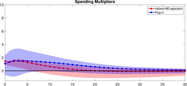
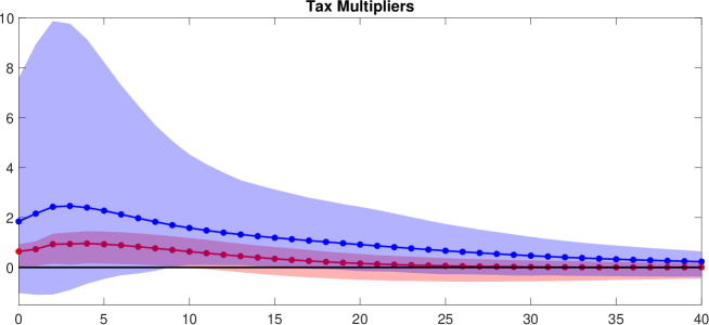
Figure S.1: Fiscal multipliers. Red dotted lines correspond to the multipliers estimated with our indirect-MD approach; red shaded areas are the corresponding 68% MBB confidence intervals; blue dotted lines correspond to the Plug-in multipliers obtained pretending that the proxies $z_{t}^{tax}$ and $z_{t}^{g}$ (direct approach) are strong for the tax and spending shocks; blue shaded areas are the corresponding 68% Plug-in confidence intervals.