A survey of Identification and mitigation of Machine Learning algorithmic biases in Image Analysis

Abstract

The problem of algorithmic bias in machine learning has gained a lot of attention in recent years due to its concrete and potentially hazardous implications in society. In much the same manner, biases can also alter modern industrial and safety-critical applications where machine learning are based on high dimensional inputs such as images. This issue has however been mostly left out of the spotlight in the machine learning literature. Contrarily to societal applications where a set of proxy variables can be provided by the common sense or by regulations to draw the attention on potential risks, industrial and safety-critical applications are most of the times sailing blind. The variables related to undesired biases can indeed be indirectly represented in the input data, or can be unknown, thus making them harder to tackle. This raises serious and well-founded concerns towards the commercial deployment of AI-based solutions, especially in a context where new regulations clearly address the issues opened by undesired biases in AI. Consequently, we propose here to make an overview of recent advances in this area, firstly by presenting how such biases can demonstrate themselves, then by exploring different ways to bring them to light, and by probing different possibilities to mitigate them. We finally present a practical remote sensing use-case of industrial Fairness.

Keywords Machine Learning, Trustworthy AI, Fairness, Computer Vision, Bias Detection, Bias Mitigation

1 Introduction

The ubiquity of Machine Learning (ML) models, and more specifically deep neural network (NN) models, in all sorts of applications has become undeniable in recent years. From classifying images [1, 2, 3], detecting objects [4, 1] and performing semantic segmentation [5, 4] to translating from one human language to another [6] and doing sentiment analysis [7], the advances in different subfields of ML can be attributed mostly to the explosion of computing power and their ability to speed up the training process of artificial NNs. Most famously, AlexNet [8] allowed for an impressive jump in performance in the challenging ILSVRC2012 image classification dataset [1], also known as ImageNet, permanently cementing deep convolutional NN (CNN) architectures in the field of computer vision. Since then, architectures have gotten more refined [9, 10], training procedures have gotten increasingly more complex [11], and their performance and robustness have greatly improved as a consequence. Namely, the success of these deep CNN models is related to their ability to treat high-dimensional and complex data such as images or natural language. The impressive performance of NNs for machine learning tasks can be explained by the ability of their flexible architecture to capture meaningful information on various kinds of complex data and the fact that they are potentially composed of millions of parameters.

However, this poses a major challenge: deciphering the reasoning behind the model’s predictions. For instance, typical NN architectures for classification or regression problems incrementally transform the representation of the input data in the so-called latent space (or feature space) and then use this transformed representation to make their predictions, as summarized in Fig. 1. Each step of this incremental data processing pipeline (or feature extraction chain) is carried out by a so-called layer, which is mathematically a non-linear function (blue rectangle in Fig. 1). It is typically made of a linear transformation followed by a non-linear activation function [12, 9], but more complex alternatives exist – e.g. the residual block layers of ResNet models [10] or the self-attention layers [13] in transformer models. These first stages of the model (Fig. 1) often rely on the bottlenecking of the information that’s passing through it by sequentially decreasing the size of the feature maps and applying non-linear transformations – e.g. the widely used ReLU activation function [14]. To summarize, these first stages project the input data into a latent space. Therefore, the neural network’s data extraction pipeline is driven by the training data that were used to optimize its parameters. The second part of the network (Fig. 1), which is standard for classifiers or regressors, is generally simpler to understand than the first, as it is often composed of matrix-vector products (often denoted as dense or fully-connected layers) followed by ReLU activation functions. Consequently, it is mathematically equivalent to a piece-wise linear transformation [15]. More importantly, these non-linear transformations depend on parameters that are optimized to make accurate predictions for a particular task when training the NN.

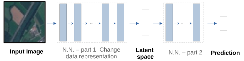
Figure 1: General architecture of a neural network designed for classification or regression tasks on images. It first non-linearly projects the input image information into a latent space, and then uses this transformed information for its prediction.

Finally, it is worth emphasizing that the data transformation from the latent space to the NN’s output can be as complex as in the first part of the network Fig. 1 in models that are not designed for regression or classification, such as e.g. the unsupervised auto-encoder models [16] or U-Nets [17]. This makes their analysis and control even more complex than in models following the general structure of Fig. 1.

The fact that neural networks are black-box models raises serious concerns for applications where algorithmic decisions have life-changing consequences, for instance in societal applications or for high risk industrial systems. This issue has motivated a substantial research effort over the last few years to investigate both explainability, and the creation and propagation of bias in algorithmic decisions. An important part of this research effort has been made to explain the predictions of black-box ML models [18, 19, 20, 21] or to detect out-of-distribution data [22, 23].
In this paper we will leverage the significant work that has been made in the field of Fairness, and study how it can be extrapolated to industrial computer vision applications. Fairness in Machine Learning considers the relationships between an algorithm and a certain input variable that should not play any role in the model’s decision from an ethical, legal or technical point of view, but has a considerable influence on the system’s behavior nonetheless. This variable is usually called the sensitive variable. Different definitions have been put in the statistical literature, each of them considering specific dependencies between the sensitive variable and the decision algorithm. From a more practical point of view, Fairness issues in Machine Learning manifest themselves in the shape of undesired algorithmic biases in the model’s predictions, such as according more bank mortgages to males than females for similar profiles or hiring males rather than females for some specific job profiles, due to a majority presence of male individuals with the corresponding profile in the learning database. Hence, Fairness initially gained a lot of attention specifically in social applications, with a large amount of articles speaking out about the different types of bias that ML algorithms amplify. We refer for instance to the recent review papers of [24, 25] and references therein.

However, we want to emphasize that studies focusing on the presence of bias in more general industrial applications based on complex data like images have mostly been left out of the spotlight. We intend to raise awareness about this kind of problem for safety-critical and/or industrial applications, where trained models may be discriminating against a certain group (or situation) in the form of a biased decision or diminished performance. We point out that a team developing a NN-based application might simply be unaware of this behavior until the application is deployed. In this case, specific groups of end-users may observe that it does not work as intended. A typical example of undesired algorithmic bias in image analysis applications is the one that was made popular by the paper presenting the LIME explainability technique [20]. Indeed, the authors trained a neural network to discriminate images representing wolves and huskies. Despite the NN’s reasonable accuracy, it was still basing itself off spurious correlations – i.e. the presence or not of snow in the background – to decide whether the image contained a wolf. Another example that will be at the heart of this paper is a blue veil effect in satellite images, which will be discussed in Section 5. When present, these biases provide a shortcut for the models to achieve a higher accuracy score both in the training and test datasets, although the logic behind the decision rules is generally false. This phenomenon is often modeled by the use of confounding variables in statistics. Hence, they hinder these models’ performance when predicting a sample from the discriminated group. This makes it completely clear that all harmful biases must be addressed in industrial and safety-critical applications, as algorithmic biases might render the general performance guarantees useless in specific or uncommon situations.

We make the following contribution in this survey:

• We summarize different types of bias and fairness definitions most commonly present for images.

• We present a comprehensive review of methods to detect and mitigate biases with a particular focus on machine learning algorithms devoted to images.

• We identify open challenges and discussing future research direction around an industrial use case of image analysis.

2 Fairness in Machine Learning

In this section, we will briefly introduce the different definitions of Fairness that we will consider in this paper. In particular, we will concentrate on statistical – or global – notions of Fairness that are the most popular among ML practitioners. There exist other definitions based on causal mechanisms that provide a local measure of discrimination [26] or [27] – and that play an important role in social applications, where discrimination can be assessed individually –, but they are beyond the scope of this paper.

2.1 Definitions

Let $X$ be the observed input images, $Y$, the output variables to forecast and $A$, the sensitive variable that induces an undesirable bias in the predictions (introduced in Section 1), which can be explicitly known or deduced from $(X,Y)$. In a supervised framework, the prediction model $f_{\theta}$ is optimized so that its parameters $\theta$ minimize an empirical risk $R(Y,\hat{Y})$, which measures the error of forecasting $Y$, with $\hat{Y}:=f_{\theta}(X)$. We will denote $\mathcal{L}(Z)$ the distribution of a random variable $Z$.

An image is defined as an application $X:K_{1}\times K_{2}\mapsto\mathbb{R}^{d}$, where $K_{1}$ and $K_{2}$ are two compact sets representing the pixel domain ($K_{3}$ and $k_{4}$ can also be considered for 3D or 3D+t images) and $d$ is the number of image channels (e.g. $d=3$ for RGB images). We will consider 2D images with $d=1$ in the remainder of this section to keep the notations simple. An image can thus be interpreted as an application mapping each of its coordinates $(i,j)$ to a pixel intensity value $X(i,j)$. Metadata, denoted here by ${\rm meta}$, can also be associated to this image. They represent its characteristics or extra information such as the image caption, its location, or even details on the sensor(s) used to acquire or to register it. In a ML setting, the variable to forecast is the output observation $Y$. Fairness is usually assessed with respect to a variable called the sensitive variable $A$ which may be either a discrete variable or a continuous variable. In the discrete case, Fairness objective is to measure dissimilarity in the data and/or discover differences in the algorithm’s behavior between samples having different sensitive variable values – i.e. corresponding to different subgroups. Thus, a complete dataset contains the images $X$, their corresponding target variables $Y$, image metadata ${\rm meta}$ and the sensitive variable $A$.

Bias can manifest itself in multiple ways depending on how the variable which causes the bias influences the different distributions of the data and the algorithm.

Bias can originate from the mismatch between the different data distributions in the sense that small subgroups of individuals have different distributions, i.e $\mathcal{L}(Y,X|A)\neq\mathcal{L}(Y,X)$. This is the most common example that we can encounter in image datasets. The first consequence can be a sampling bias, and can discourage the model from learning the particularities of the under-represented groups or classes. As a consequence, despite achieving a good average accuracy on the test samples, the prediction algorithm may exhibit poor generalization properties when deployed on real life applications with different subsets of distributions.

Another case emerges when external conditions that are not relevant for the experiment induce a difference in the observed data’s labels in the sense that $\mathcal{L}(Y|X,A)\neq\mathcal{L}(Y|X)$, therefore inadvertently encouraging models to learn biased decisions (as in the Wolves versus Huskies example in [20]). This is the case when data is collected with labels influenced by a third unknown variable leading to confounding bias, or when the observation setting favors one class over the other leading to selection bias. The sources of this bias may be related to observation tools, methods or external factors as it will be pointed out later.

A third interesting case concerns the bias induced by the model itself, which is often referred to as inductive bias: $\mathcal{L}(\hat{Y}|X,Y,A)\neq\mathcal{L}(\hat{Y}|X,Y)$. This opposes the world created by the algorithm – i.e. the distribution of the algorithm outputs – to the original data. From a different point of view, bias can also arise when the different categories of the algorithm outputs differ from the categories as originally labeled in the dataset – i.e. $\mathcal{L}(Y|\hat{Y},X,A)\neq\mathcal{L}(Y|\hat{Y},X)$ – a condition that is often referred to as lack of sufficiency.

Finally, the two previous conditions can also be formulated by considering the distribution of the algorithm prediction errors and their variability with respect to the sensitive variable: $\mathcal{L}(\ell(Y,\hat{Y})|X,A)\neq\mathcal{L}(\ell(Y,\hat{Y})|X)$, where $\hat{Y}\times Y\mapsto\ell(\hat{Y},Y)$ is the loss function measuring the error incurred by the algorithm by forecasting $\hat{Y}$ in place of $Y$.

2.2 Potential causes of bias in Computer Vision

In practice, the above described situations may materialize through different causes in image datasets.

2.2.1 Improperly sampled training data

First, the bias may come from the data themselves, in the sense that the distribution of the training data is not the ideal distribution that would reflect the desired behavior that we want to learn. Compared with tabular data, image datasets can be difficult to collect, store and manipulate due to their considerable size and the memory storage they require. Hence, many of them have proven to lack diversity – e.g. because not all regions are studied (geographic diversity), or not all sub-population samples are uniformly collected (gender or racial diversity). The growing use of facial recognition algorithms in a wide range of areas affecting our society is currently debated. Indeed, they have demonstrated to be a source of racial [28, 29], or gender [30] discrimination. Besides, well-known datasets such as CelebA [31], Open Images [32] or ImageNet [1] lack of diversity – as shown in [33] or [34] – resulting in imbalanced samples. Thus, state-of-the-art algorithms are unable to yield uniform performance over all sub-populations. A similar lack of diversity appear in the newly created Metaverse as pointed out in [35] creating racial bias. This encouraged several researchers to design datasets that do not suffer from these drawbacks – i.e. preserving diversity – as illustrated by the Pilot Parliament Benchmark (PPB) dataset [36] or in [37] or in Fairface dataset [38].

Combining diverse databases to get a sufficient accuracy in all sub-populations is even more critical for high-stakes systems, like those commonly used in Medicine. The fact that medical cohorts and longitudinal databases suffer from biases has been long ago acknowledged in medical studies. The situation is even more complex in medical image analysis for specialties such as radiology (National Lung Screening Trial, MIMIC-CXR-JPG [39], CheXpert [40]) or dermatology (Melanoma detection for skin cancer, HAM10000 database [41]), where biased datasets are provided for medical applications. Indeed, under-represented populations in some datasets lead to critical drop of accuracy, for instance in skin cancer detection as in [42], [43] or for general research in medicine [44] and references therein.

The captioning of images is a relevant example where shortcoming of diversity hampers the quality of the algorithms’ predictions, and may result in biased forecasts as pointed out in [45] or in [46]. Therefore, it is of utmost importance to include diversity (e.g geographic, social, ..) when building image datasets that will be used as reference benchmarks to build and test the efficiency of computer vision algorithms.

2.2.2 Spurious correlations and external factors

The context in which the data is collected can also create spurious correlations between groups of images. Different acquisition situations may provide different contextual information that can generate systematic artifacts in specific kinds of images. For instance, confounding variables such as the snowy background in the Wolves versus Huskies example of [20] (see Section 1) may add bias in algorithmic decisions. In this case, different objects in images may have similar features due to the presence of a similar context, such as the color background, which can play an important role in the classification task due to spurious correlations. We refer to [47] for more references. This phenomenon is also well known in biology where spectroscopy data are highly influenced by the fluorescence methods as highlighted in [48], which makes machine learning difficult to use without correcting the bias. Different biases related to different instruments of measures are also described for medical data in [49].
An external factor can also induce biases and shift the distributions. It is important to note that all images are acquired using sensors and pre-processed afterwards, potentially introducing defects to the images. In addition, their storage may require to compress the information they contain in many different ways. All this makes for a type of data with a considerable variability depending on the quality of the sensors, pre-processing pipeline and compression method. This will be illustrated in the application of Section 5, where an automatic pre-processing scheme induces a bias in pseudo-color satellite images. In medical image analysis, external factors such as age affect the size of the organs but is also a causal factor to some diseases as analyzed in [50], for instance.

2.2.3 Unreliable labels

We can finally note that wrong or noisy labels, bad captioning (due to stereotyping, for instance) or the use of labeling algorithms that already contain bias (such as Natural Language Processing image interpreters) are also potential source of bias. An example of this phenomenon can be the subjective and socially biased choice of the attractive labels in the CelebA [31] dataset. When image datasets include captioning as additional variable, the bias inherent to learned language model used to provide the caption is automatically included. For instance one of the main pre-trained algorithm in Natural Language Processing, Generative Pre-Trained Transformer 3, a.k.a GPT-3, is well known to be biased and thus generalized its bias to the image datasets as described for instance in [51] for gender bias.

2.3 From determined bias to unknown bias in image analysis

Keeping in mind the potential sources of bias, different situations may also occur in image analysis applications, depending on the availability of the information:

• Full information: images, targets, metadata and sensitive variables, i.e. $(X,Y)\cup\>\{{\rm meta}\}\>\cup A.$ are available. The bias may then come from the meta-observations $\{{\rm meta}\}$, the image itself, the labels, or all three.

• Partial information: the sensitive variable is not observed, so we only observe $(X,Y)\cup\>\{{\rm meta}\}$. The sensitive variable may be included in the meta variables $A\subset\{{\rm meta}\}$, or may be estimated using the meta-variables $\{{\rm meta}\}$.

• Scarce information: only the images are observed along with their target, i.e. we only observe $(X,Y)$. The sensitive variable $A$ is therefore hidden. The bias it induces is contained inside the images and has to be inferred from the available data $X$ and used to estimate $A$.

For societal applications, the sensitive variable is defined following regulations as presented in Section 2.4. The variable $A$ is known since it is chosen by the regulator, and hence, is either directly available in the data or proxies can be found to estimate it. The main difficulty when working with high dimensional inputs such as images (but also natural language data, time series or graphs) is that the bias may not be explicitly present in a particular input dimension or variable, but is rather hidden in a latent representation of the input data. For instance, an image-based classifier would not naturally have a different rate of positive decisions for males and females because of the intensity of a specific pixel. It would instead detect specific patterns or features in the input images and potentially use this information, leading to unfair decisions with respect to a gender sensitive variable. As discussed in Section 1, neural network classifiers or regressors change by construction the representation of the input data into a lower dimensional latent (or feature) space before making their predictions based on this latent information. Illustrations of how a network can project the input information in a latent space can be found in the VGG and ResNet papers [9, 10]. It would then be tempting to believe that the hidden variables explaining the undesirable biases would be found in the latent space but this is not necessarily the case. This information can still be distilled in different latent variables unless a specific process is made to isolate it [52]. Hence, bias detection is an essential, potentially arduous task when dealing with images.

2.4 Current regulation of AI

It is interesting to remark that the social concerns related to a massive use of AI systems in modern societies has lead to the definition of various ethical and human rights-based declarations intending to guide the development and the use of these technologies. Some of them were defined by governments or inter-governmental organizations, other ones raised from the civil society, private companies or multi-stakeholders. In 2020, the particularly interesting work of [53] compared the contents of 36 prominent AI principal documents side-by-side. This made clear the similarities and differences in interpretation across these frameworks. This also emphasized the fact that an AI system can be considered as unfair with respect to the ethic principles of one of these documents but fair for another one, which can be particularly confusing for end-users. In order to ensure the trust of the users in AI systems and to properly regulate the use of AI, different states or unions now define specific laws for the use of AI. For instance, the so-called AI act of the European Commission will require AI systems sold or developed in the European Union to have proper statistical properties with regard to potential discrimination they could engender (see articles 9.7, 10.2, 10.3 and 71.3). It is also worth mentioning that the article 13.1 of this proposal suggests that the decisions of the AI systems that are likely to pose high risks to fundamental rights and safety (see Annex III of the proposal) may be sufficiently transparent to enable users to interpret the system’s output. Making sure that each individual decision can be interpreted by the user is a central question addressed by explainable AI, and is the key to understanding whether a specific decision is made by only exploiting pertinent and insensitive information in the input data, or not. As a direct consequence, the user can assess whether an individual decision is fair or not. The sanctions for non-respect of these rules should have a deterrent effect in the E.U. as they can be as high as 30 million euros or 6% of a company annual turnover (see Article 71).

These regulations directly involve various applications of image analysis as they might fall into the category of high-risks systems such as medical imaging [54, 55, 56, 57] or even facial recognition algorithm [58, 59, 60] as they might relate to people daily life.

3 Bias detection

Different methods were proposed to detect such (undesired) algorithmic biases in machine learning. After presenting the main Fairness metrics, we will give an overview of the recent methods that can be used to detect unknown (or non referenced) biases.

3.1 Fairness metrics

A large variety of fairness metrics have been introduced to quantify algorithmic biases, as presented in [61, 62, 63, 25] and references therein. They quantify different levels of relationships between a given sensitive variable $A$ and outputs of the algorithm. Yet, as fairness is a polysemous word, there exist multiple metrics, each one focusing on a particular definition of bias and, unfortunately, all of them are not necessarily compatible with each other, as recently discussed in [24] or [64]. Therefore, it is essential for someone evaluating the bias of a model to understand what the fairness metrics really capture. They conform to different definitions of biases given in the previous section and can be decomposed as follows.

Statistical parity

One of the most standard measures of algorithmic bias is the so-called Statistical Parity. Fairness in the sense of Statistical Parity is then reached when the model’s decisions are not influenced by the sensitive variable value – i.e. $\mathcal{L}(\hat{Y}|A)=\mathcal{L}(\hat{Y})$. For a binary decision, it is often quantified using the Disparate Impact (DI) metric. Introduced in the US legislation in 1971 it measures how the outcome of the algorithm $\hat{Y}=f_{\theta}(X)$ depends on $A$.
It is computed for a binary decision as

$$DI(f)=\frac{\mathbb{P}(f_{\theta}(X)=1|A=0)}{\mathbb{P}(f_{\theta}(X)=1|A=1)}\,,$$

where $A=0$ represents the group which may be discriminated (also called minority group) with respect to the algorithm. Thus, the smaller the value, the stronger the discrimination against the minority group; while a $DI(f)=1$ score means that Statistical Parity is reached. A threshold $\tau_{0}=0.8$ is commonly used to judge whether the discrimination level of an algorithm is acceptable [65, 66, 67].

Equal performance metrics family

Taking into account the input observations $X$ or the prediction errors can be more proper in various applications than imposing the same decisions for all. To address this, the notions of Equal performance, Status-quo preserving, or Error parity measure whether a model is equally accurate for individuals in the sensitive and nonsensitive groups. As discussed in [24], it is often measured by using three common metrics: Equal sensitivity or Equal opportunity [61], Equal sensitivity and specificity or Equalized odds, and Equal positive predictive value or Predictive parity [68]. In the case of a binary decision, common metrics usually compute the difference between True Positive Rate and/or False Positive Rate for majority and minority groups. Therefore, Fairness in the sense of Equal performance is reached when this difference is zero. Specifically: An Equal opportunity metric is given by

$$|\mathbb{P}(\hat{Y}=1|A=0,Y=1)-\mathbb{P}(\hat{Y}=1|A=1,Y=1)|\,,$$

while an Equality of odds metric is provided by

$$|\mathbb{P}(\hat{Y}=1|A=0,Y=0)-\mathbb{P}(\hat{Y}=1|A=1,Y=0)|.$$

Finally, Predictive parity refers to equal accuracy (or error) in the two groups. Previous notions can be written using the notion of calibration in fairness. When the algorithm’s decision is based on a score $s(X)$, as in [69], a Calibration metric is defined as

$$|\mathbb{P}(Y=1|A=0,s(X))-\mathbb{P}(Y=1|A=1,s(X))|.$$

Calibration measures the proportion of individuals that experience a situation compared to the proportion of individuals forecast to experience this outcome. It is a measure of efficiency of the algorithm and of the validity of its outcome. Yet studying the difference between the groups enable to point out difference of behaviors that would let the user to trust the outcome of an algorithm less for one group than another. This definition extends in this sense previous notions to the multi-valued settings as pointed in [70]. Calibration is similar to the definition of fairness using quantile developed in [71].

Note that previous definitions can easily be extended to the case where the variables are not binary but discrete.

Advanced metrics

First, for algorithms with continuous values, previous metrics can be understood as quantification of the variability of a mean characteristics of the algorithm, with respect to the sensitive value. So natural metrics as in [72] or [73] are given by

$${\rm Var}E[f_{\theta}(X)|A]\quad\mathrm{or}\quad{\rm Var}E[\ell(f_{\theta}(X),Y)|A]$$

Note that as pointed in [72], these two metrics are unnormalized Sobol indices. Hence, sensitivity analysis metrics can also be used to measure bias of algorithmic decisions. As a natural extension, sensivity analysis tools provide new ways to describe the dependency relationships between a well chosen function of the algorithm, focusing on particular features of the algorithm. They are well adapted to studying bias in image analysis.

Previous measures focus on computing a measure of dependency. Yet, many authors used different ways to compute covariance-like operators, directly as in [66], or based on information theory [74], or using more advanced notions of covariance based on embedding, possibly with kernels. We refer for instance to [63] for a review. Each method chooses a measure of dependency and computes a fairness measure of either the outcome of the algorithmic model or its residuals (or any appropriate transformation) with the sensitive parameter.
Other measures of fairness do not focus on the the mean behavior of the algorithm but other properties that may be the quantiles or the whole distribution. Hence, fairness measures compare the distance between the conditional distribution for two different values of the sensitive attribute $a\neq a^{\prime}$ of either the decisions

$$d(\mathcal{L}(f_{\theta}(X)|A=a),\mathcal{L}(f_{\theta}(X)|A=a^{\prime}))$$

or their loss

$$d(\mathcal{L}(\ell(f_{\theta}(X),Y)|A=a),\mathcal{L}(\ell(f_{\theta}(X),Y)|A=a^{\prime})).$$

Different distances between probability distributions can be used. We refer for instance to [75] and references therein, where Monge-Kantorovich distance (aka Wasserstein distance) is used. Embedding of distributions using kernels can also be used as pointed out in [76], together with well adapted notions of dependency in this setting.

3.2 Unknown bias detection

We now present different methods to detect unknown bias, or more precisely, algorithmic bias with respect to sensitive variables that have to be estimated. In essence, there are two veins in the bias detection literature: testing for the presence of a suspected bias in the model, and the discovery of sources of bias without supervision. For the former, the emphasis will be put on the structure of the trained model, whereas notions of statistical and counterfactual fairness – with the help of generative models – and explainability techniques will be the center point for the latter. Although fairly new and not yet popularized in the fairness literature, the topic of bias detection is of particular interest for image-based applications, as discussed in Section 2.2 and 2.3. The combinatorial problem itself of identifying groups of samples without any domain knowledge or prior about what constitutes an informative representation for a specific use-case is ill-posed. This is why the techniques presented below leverage semantic information in some way or another to identify potentially discriminated groups.

In  [77], Serna et al. proposed to study the values of the activations in CNNs for a facial gender recognition task, and discover that when the models have learned a biased representation, the activations in its filters are not as high when dealing with samples from the discriminated groups. In  [78], the same group of researchers extended this work by training different groups of NNs, and then used other models to predict the presence of bias from their weights without looking at their inferences, proving that bias is encoded in the model’s weights. Other works also interestingly investigate the predictor’s hidden activations to detect sub-groups [79, 80, 81, 82].

In [83], Denton et al. used generated counterfactual examples to discover and assess unknown biases. By supposing that a generative model was available, they generated counterfactual examples given a set of interpretable attributes, and tested the performance of a trained classifier. A significant drop of the classifier performance was then considered as a good indicator that a specific attribute used to generate the counterfactual example was highly influential, and could therefore reveal an unintended bias. In much the same manner, Li et al.  [84] proposed to discover unknown biased factors in a classifier by generating factor traversals with generative models and a special hyperplane optimization. In this method, the classifier and the generative models have their weights fixed, i.e. they are already trained, so only the hyperplane is optimized thanks to the model outputs. Thus, images traversals are generated with more and more relevance with respect to orthogonal dimensions and largest variations on the classification scores. We can also highlight the work of Paul et al. [85] which expand the scope of fairness from focusing solely on demographic factors to more general factors by using generative models that discover them.

By exploiting the widely known GradCAM method [18], Tong and Kagal [86] recover the image classification model properties when making a decision. Their intuition is that the results could expose biases learned by the model. For example, in a dataset where most of doctors are males, GradCAM exposed the fact that the model’s predictions focused mainly on the facial features of the person, while clothes and accessories are highlighted for female doctors. The same conclusions were drawn for basketball players, where GradCAM explained that the predictions were mainly based on the players’ faces and not on basketball-related features. Although the predictions were often accurate, explanations made indeed clear that they were based on players’ faces because the training dataset contained a lot of female volleyball players, and facial features help a lot to predict a person gender. Finally, Schaaf et al. [87] combined attribution methods with ground truth masks to help detecting biases.

It is important note that the models were trained with labels in all above-mentioned methods, but biases might still be learned when using self-supervised training schemes. In [88], Sirotkin et al. looked for the presence of bias in representations learned using state-of-the-art self-supervised learning (SSL) procedures. In particular, they pre-trained models on ImageNet [1] using a variety of SSL techniques and showed that there was a correlation between the type of model and the number of incorporated biases. Thus, they demonstrated that biases can be learned even without supervision. In a Meta-Learning fashion, [89] also propose to learn how to split a dataset such that predictors learned on a training split which cannot generalize on the test split.

4 Obtaining fairness

Obtaining fairness of an algorithm has been studied for a large number of applications, most of them dealing with societal problems where bias induces a potential harm for the populations, leading to potential discrimination. Hence, mitigating the bias is focuses on obtaining algorithms which perform similarly for all groups in a population. Although similar in some cases to the notions of fairness that are typically used in social applications – e.g. captioning [90] or predictive policy [91] –, Fairness can have slightly different goals in industrial applications,.

• Firstly, it is critical to obtain robust algorithms that generalize to the test domain with a certified level of performance, and that do not depend on specific working conditions or types of sensors to work as intended. The property which is sought is the robustness of the algorithm.

• Secondly, the second goal is to learn representations independent of non-informative variables that can correlate with actual predictive information and play the role of confounding variables. The relationship between Fairness and these representations constitutes an open challenge. In many cases, representations are affected by spurious correlations between subjects and backgrounds (Waterbirds, Benchmarking Attribution Methods), or gender and occupation (Athletes and health professionals, political person) that influence too much the selection of the features, and hence, the algorithmic decision. One way of studying it, is through disentangled representations [52]: by isolating each factor of variation into a specific dimension of the latent space, it is possible to ensure the independence with respect to sensitive variables.

Once a source of undesirable bias has been identified, a mitigation scheme should be implemented to avoid unreliable model behaviors in certain regions of the input space. For example, it has been shown that when generating explanations on discriminated groups, the standard post-hoc explainability methods score significantly lower than when applied to samples belonging to non-discriminated groups [92, 93]. This means that fairness can be a requisite to ensure that all the properties verified by our models on majority groups are still valid for minority groups. This is particularly pertinent in industrial and safety-critical applications, where some properties can be required for the system’s certification. In this case, new notions of fairness can be derived from these criteria, leading to new definitions of statistical equality implying that the properties are satisfied for all sub samples of the data.

Bias correction techniques can be divided into two categories depending on whether they are intended to be applied to problems in which the bias is already known or not. When this is the case, state-of-the-art methods mostly work by erasing the information related to the sensitive variable present in the latent space, or re-sampling/re-weighting the training dataset, or generating samples via generative models. Through the former, the latent space is split into predictive and sensitive information, and only the first part is used to learn how to predict. In contrast, by working with the training samples, the latter attempts to give more importance to under-represented groups during the training phase.

All these methods require access to the group’s labels at train time, condition which might not be met on certain use-cases. It is also interesting to note that existing group labels may alternatively not be informative of actual harmful biases. Different methods were then proposed to treat these more complex cases. They can be based on either proposing potential confounding variables [94], or on approaches from the field of Distributionally Robust Optimization (DRO) [95]. In particular, this latter family of methods has been a focal point for the emerging field of sub-population shift, or group shift, whereby the training distribution can be subdivided into multiple groups (oftentimes without labels) and the test distribution becomes the one of the group on which the model performs the worst.

When group labels are available at training time, the problem is well-posed and the algorithmic bias that the studied models have learned can be erased. For instance, in [96], Zhang et al. proposed to employ an adversarial network to modify the latent space of the classifier to optimize a given fairness metric. In a similar way, Kim et al. [97] used an adversary to minimize the mutual information between the latent space and the sensitive variable. Grari et al. [98] also adversarially optimized the Hirschfeld-Gebelein-Rényi (HGR) maximal correlation coefficient. Penalty terms were also used in [75, 66] to ensure a good balance between model accuracy and fairness properties with respect to a sensitive variable. In a somewhat different path, other techniques piggyback on the fact that disentangled representations can be more fair than standard ones, as the important information for the prediction is separated from the sensitive variable [52]. In particular, this has been applied in [99, 100] to split the latent space into two groups through the use of specific losses, with the task information on one side and the sensitive variable on the other.

It is also possible to encourage models to learn fair representations by only using the data. Among the simplest methods, a reweighting factor can be added to the loss so as to emphasize the discriminated samples [101]. An alternative is to resample the training dataset in different manners: by undersampling the dominant groups to encourage the model to learn more general rules [102], by oversampling the discriminated groups [103], by using a technique similar to MixUp [104] to interpolate between dominant and minority groups [105], or by generating more samples of the discriminated groups through generative models [106, 107, 108].

When the sensitive variable is not available, previous methods can not be used. The literature dealing with unknown bias is scarce, yet some solutions can be found in the machine learning literature. As in previous sections, mitigation of unknown bias amounts to correct the data or the algorithm from features that influence the algorithm. Yet from feature detection to bias mitigation, there is a gap that requires some additional knowledge that allows us to decide whether a particular direction corresponds to a bias that has to be avoided or not.

When humans are in the loop, or if the data can be described using logical variables, bias mitigation can be handled by using orthogonality constraints that prevent dependencies as in [109]. When some causal information is available such as a causal graph for instance, Variational Auto-Encoders can be trained to infer some proxy for the sensitive variable as in  [110]. The information required is that some part of the variable are independent from the sensitive variable while the other part may be highly correlated.

Then, when the groups are unknown but the training data are known to not be completely unbiased, there are still different approaches to help improve the worst-case performance. Namely, it is possible to propose group labels without supervision through clustering, and then apply a reweighting scheme [94].

In all previous settings, the bias implies that the algorithm generalizes poorly to new datasets. In particular, this is the case when variations of the sensitive variable produce changes in the data distributions. Hence, algorithms that are able to achieve a good level of performance for different testing distributions are, by nature, able to handle this type of bias. Distribution Robustness of the algorithm can induce fairness in this sense. The DRO framework corresponds to solving the minimax problem

$$\min_{\theta\in\Theta}\max_{Q\in\mathcal{Q}}\mathbb{E}_{Q}\left[\ell(Y,f_{\theta}(X)\right]$$

where $\mathcal{Q}$ is a set of distributions close to the empirical training distribution $\mathbb{P}_{n}$ that we call the uncertainty set. The choice of this $\mathcal{Q}$ establishes how the training distribution can be perturbed, with most techniques choosing all the distributions such that a f-divergence [95, 111] or a Wasserstein distance [112] is smaller than a certain threshold, or by modeling it with a generative network [113]. If some causal information is available and if, so called interventions on the sensitive variable, can be modeled as distributional shifts on the distributions, hence distributional robust models with respect to such shifts will be protected from the bias induced by this variable. Therefore, distributional robustness extends stability requirements to achieve fairness by controlling the output of the algorithm in the worst distributional case around the observed empirical distribution.

5 A use-case for EuroSAT

We now illustrate the notions and concepts of algorithmic bias that can be encountered in industrial applications on the RGB version of the EuroSAT dataset [3]. It contains 27000 remote sensing images of $64\times 64$ pixels with a ground sampling distance of 10 meters. The RGB channels were also reconstructed based on the original 13-band Sentinel-2 satellite images. Each image has a label indicating the kind of land it covers, as shown in Fig. 2-(left).

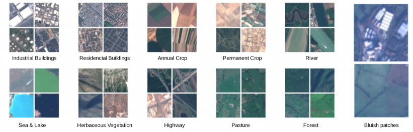
Figure 2: (Left) Images out of the 10 classes of the EuroSAT dataset. Illustration taken from [3] (Right) Images of the EuroSAT dataset for which the reconstruction in the RGB color space produced the blue-veil effect.

.

5.1 The blue veil effect in the EuroSAT dataset

The blue-veil effect is caused by uncommon atmospheric conditions when acquiring Sentinel-2 images on the original 13 spectral bands, and becomes particularly noticeable when they are transformed into the visible spectrum. In essence, the picture acquires a blueish hue, as depicted in Fig. 2-(right), that can trick classification models into thinking that it contains a mass of water. About 3% of the dataset is corrupted by what we call the blue-veil effect. Importantly, this blue-veil effect will provide us below a typical example of algorithmic bias with an unknown sensitive variable in high-dimensional data. As we will see, blue-veil images indeed tend to be harder to classify than other images.

5.2 Detecting sensitive variables without additional metadata

We explain hereafter how to detect the blue-veil effect as a potential source of bias. The first step is to estimate the importance of each observation of the training dataset for a pre-trained model. This information will then be employed by clustering algorithms on specific image representations in order to automatically find the discriminated group.

We opted for the technique of [114], where first order approximations of NN influence functions were used to determine the importance of each training observation in the trained model. With this objective in mind, a simple and generic 4-layer CNN was trained until convergence. Then, we observed that among the 25 most influential images, 7 of them were blue-veiled images, although such images only represent 3% of the whole dataset. This suggests that training the classifier on blue-veil images is a complex task, or at least that the image features used to classify these images seem to be different than those of the other images.

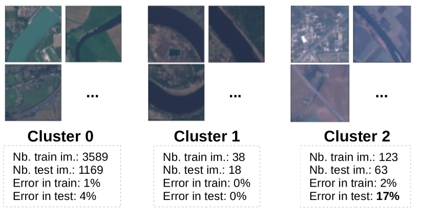
Figure 3: Detection of potentially discriminated groups and confirmation of blue-veiled images using a clustering and group-wise performance evaluation methodology. The generalization properties of a ResNet18 classifier in cluster 2, i.e. for blue-veil images, are particularly lower than in the two other clusters.

Since the blue-veil pattern has been semi-automatically identified on several images, we can change the image representation so that a clustering algorithm will straightforwardly find and isolate all the images with this pattern in the training and test sets. For the blue-veiled images, we simply transform the RGB (Red, Green, Blue) color space into an HSV (Hue, Saturation, Value) space, where the blue-veil images can be characterized by dominant blue colors in the Value channel and reasonably luminous colors in the Hue channel. By using a spectral clustering algorithm on HSV images, we distinguish three image clusters, as shown Fig. 3. The first cluster contains normal-looking images, the second one mostly has large and dark rivers, and a last one represents the blue-veiled images we are looking for.

5.3 Measuring the effect of the sensitive variable

Let’s check different models’ performances for blue-veiled images and other images. A simple 4-layer CNN, a VGG-16 model, and a ResNet18 model were compared after being trained for 50 epochs. A total of 10 runs per configuration were used to measure the models’ and learning algorithm’s stability. We also focused on the binary classification between Rivers and Highways, which correspond to the two worst performing classes in the 10 class setting. This additionally forced us to train the classifiers with a more limited amount of blue-veiled images, making the problem close to what we can encounter in many industrial applications. The training and test sets indeed contained 3750 and 1250 images, respectively, where only 123 and 63 images were blueish. As shown in Figures 3 and 4-(a), we can clearly observe that the error rate is considerably higher on blue-veiled images than on other images, thus demonstrating that an undesirable algorithmic bias was learned in the sense of the equality of errors.

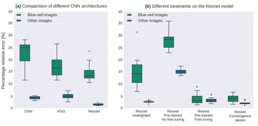
Figure 4: Average error obtained on the test set of the EuroSat dataset using different models and training strategies. For each strategy, the two boxplots distinguish the average errors on blue-veiled images (green boxplots) and other images (blue boxplots): (a) Baseline results obtained on different neural-network architectures; (b) Effect of different treatments on the average accuracy of the Resnet architecture.

5.4 Bias mitigation

Different strategies to mitigate the undesired bias on the classifiers accuracy were also compared. All techniques tested below are based on the Resnet18 architecture, as it is the one which performed best on blue-veil images (see Fig. 4-(a)). Note that we trained the models for 50 epochs by default, just like in the previous subsection. The initial parameters of the neural-networks were also randomly drawn, except in two cases that will be mentioned.

We first tested the re-weighting scheme proposed in [101]. The ResNet18 architecture was trained using a weighted loss, where the weights were chosen so that the disparate impact was equal to 1 (reweighted strategy). We also loaded the pre-trained ResNet18 architecture of Torchvision and trained its last layer on our EuroSAT data to use the generic transformed image representation of this pre-trained network. It is important to mention that a very large and generic ImageNet database was used for pre-training (Pre-trained, No fine tuning strategy). We alternatively fine-tuned all layers of this pre-trained network to simultaneously optimize the transformed image representation and the prediction based on this representation, i.e. the parts 1 and 2 of the neural-network in Fig. 1 (Pre-trained, Fine tuning strategy). It is important to note that we only trained for 5 epochs instead of 50 when fine-tuning the pre-trained neural-networks in order to avoid overfitting. Finally, we randomly drew the initial state of the neural network and trained all layers, but thoroughly distinguished the convergence for all images and for the group of blue-veiled images only. In this case, we stopped training the ResNet18 parameters when an over-fitting phenomenon started being observed in the blue-veiled images (Convergence aware strategy). Results are shown in Fig. 4-(b). A typical detailed convergence of the Convergence aware strategy is also shown in Fig. 5.

Finally, we can discuss the results. We can first notice that the re-weighting technique of [101] had little effect on the results. It was indeed designed to correct bias that manifests in the form of disparate impact, so it did not reduce the error rate gap between groups. The debiasing method must then be specifically chosen to target the bias through the metric with which it was measured. Using the pre-trained network of Torchvision had a disastrous effect when only optimizing the last neural-network layer, but was particularly efficient when using fine-tuning, i.e. when simultaneously optimizing the transformation of the data representation and the final decision rules. Using a relevant initial state, when available, and using fine tuning then appears as a very good strategy here. It is often denoted by transfer learning in the machine learning literature. Interestingly, similar results were obtained with a random initial state, when stopping the training procedure at an iteration where the trained neural-network had good generalization properties on the blue-veiled images. Understanding this result requires to look closely at the convergence curves, as illustrated Fig. 5 on a typical run:

In Fig. 5, we compare the convergence in the whole train and test sets, as well as the blue-veil images only. We can then distinguish five phases in the convergence process. All curves start decreasing in phase A. It can only be remarked that the loss on the blue-veil images slightly increases during the 4 first epochs before decreasing, as in the average trend. We believe that this is due to a minor confounding effect. In phase B, i.e. between epochs 12 and 18, the training algorithm has converged when observed on all training images but not yet on blue-veil images. This is due to the fact that the blue-veil images only represent a small fraction of the training set. Note that if only measuring the convergence on the whole training set, it would be tempting to stop the training process at the beginning of phase B, which would obviously lead to a different treatment of the blue-veiled images and other images (see $\delta$ loss 1 in Fig. 5). More interestingly for us, the convergence curves are stable on the training set in phase C, but it regularly decreases on the test set. At the end of phase C, the convergence curve is stable on the whole test set, and it is common practice to stop the training process there (early stopping principle). However, it is important to remark that the generalization properties of the trained neural-network are still much poorer for blue-veiled images than other images (see $\delta$ loss 2 in Fig. 5). This actually explains in Fig. 4-(a) the different accuracies observed for the blue-veiled images with respect to the other images. We indeed stopped the convergence after 50 epochs there. Although noisy, the convergence curve obtained on blue-veil test images slowly decreases in phase D until reaching an optimal value at epoch 145 (see $\delta$ loss 3 in Fig. 5). Finally, the training algorithm starts over-fitting the blue-veiled images in phase E, so the training process should be stopped at its very beginning. It is then essential to point out that obtaining reasonably good generalization properties on blue-veiled images required about 3 times more epochs than what is made using what’s commonly considered to be the good practices, and about 12 times more epochs than what would be made using a naive approach.

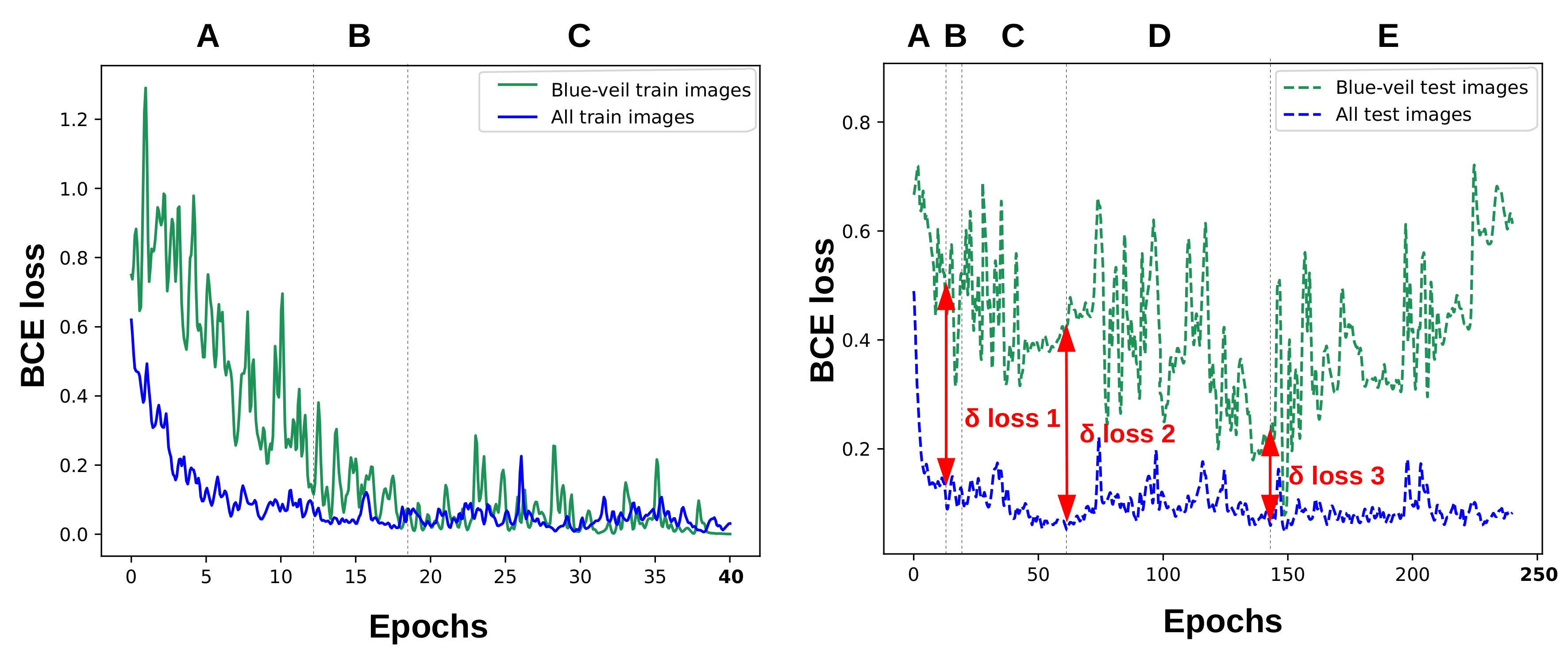
Figure 5: Detailed convergence of the BCE-loss on all data and on blue-veil images only. Results obtained on the training set (left) and on the test set (right) are represented. Note that the convergence curves obtained on the training set are only represented for the first 40 epochs, and those obtained on the test set are represented on 250 epochs. Five phases A to E are distinguished to discuss the convergence behavior.

6 Conclusion

We want to put the emphasis on the fact that undesired biases may come from a variety of unexpected reasons. While in a societal applications regulations can help to focus on specific variables, it is unfortunately most of the time an arduous task which requires awareness in the data scientists community. We proposed here to go over some techniques to characterize, detect and mitigate such undesired biases. However, we also showcased the difficulty of the task when moving forward blindly. Having a strong field expertise helps to prevent some of these hidden biases as it allows to draw the attention on specific behaviors. When such an expertise is unfortunately unavailable, practitioners should even be more cautious. Some of the works presented here did not need any prior to detect and mitigate bias but oftentimes it does not allow to exhibit clearly the source of the bias, and hence, to remove the underlying cause. Use-cases leveraging AI to its full potential are growing at an exponential pace while the advances on bias characterization unfortunately move much more slowly. Thus, we tend to believe that an in-depth work is necessary before an AI-based solution is deployed, especially to preserve the end-users’ trust. In that sense, we should see the different regulations arising as an opportunity to gain knowledge on data, deep learning, and optimization instead of a brake on innovation.

References

- [1] Jia Deng, Wei Dong, Richard Socher, Li-Jia Li, Kai Li, and Li Fei-Fei. Imagenet: A large-scale hierarchical image database. In 2009 IEEE conference on computer vision and pattern recognition, pages 248–255. Ieee, 2009.
- [2] Yann LeCun, Corinna Cortes, and CJ Burges. Mnist handwritten digit database. ATT Labs [Online]. Available: http://yann.lecun.com/exdb/mnist, 2, 2010.
- [3] Patrick Helber, Benjamin Bischke, Andreas Dengel, and Damian Borth. Eurosat: A novel dataset and deep learning benchmark for land use and land cover classification. IEEE Journal of Selected Topics in Applied Earth Observations and Remote Sensing, 12(7):2217–2226, 2019.
- [4] Tsung-Yi Lin, Michael Maire, Serge Belongie, James Hays, Pietro Perona, Deva Ramanan, Piotr Dollár, and C Lawrence Zitnick. Microsoft coco: Common objects in context. In European conference on computer vision, pages 740–755. Springer, 2014.
- [5] Marius Cordts, Mohamed Omran, Sebastian Ramos, Timo Rehfeld, Markus Enzweiler, Rodrigo Benenson, Uwe Franke, Stefan Roth, and Bernt Schiele. The cityscapes dataset for semantic urban scene understanding. In IEEE Conference on Computer Vision and Pattern Recognition (CVPR), 2016.
- [6] Philipp Koehn. Europarl: A parallel corpus for statistical machine translation. In MTSUMMIT, 2005.
- [7] Andrew L. Maas, Raymond E. Daly, Peter T. Pham, Dan Huang, Andrew Y. Ng, and Christopher Potts. Learning word vectors for sentiment analysis. In Proceedings of the 49th Annual Meeting of the Association for Computational Linguistics: Human Language Technologies, pages 142–150, Portland, Oregon, USA, June 2011. Association for Computational Linguistics.
- [8] Alex Krizhevsky, Ilya Sutskever, and Geoffrey E Hinton. Imagenet classification with deep convolutional neural networks. Advances in neural information processing systems, 25, 2012.
- [9] Karen Simonyan and Andrew Zisserman. Very deep convolutional networks for large-scale image recognition. In Yoshua Bengio and Yann LeCun, editors, 3rd International Conference on Learning Representations, ICLR, 2015.
- [10] Kaiming He, Xiangyu Zhang, Shaoqing Ren, and Jian Sun. Deep residual learning for image recognition. In Proceedings of the IEEE conference on computer vision and pattern recognition, pages 770–778, 2016.
- [11] Sergey Ioffe and Christian Szegedy. Batch normalization: Accelerating deep network training by reducing internal covariate shift. In International conference on machine learning, pages 448–456. PMLR, 2015.
- [12] Yann LeCun, Léon Bottou, Yoshua Bengio, and Patrick Haffner. Gradient-based learning applied to document recognition. In Proceedings of the IEEE, volume 86, pages 2278–2324, 1998.
- [13] Ashish Vaswani, Noam Shazeer, Niki Parmar, Jakob Uszkoreit, Llion Jones, Aidan N Gomez, Ł ukasz Kaiser, and Illia Polosukhin. Attention is all you need. In Advances in Neural Information Processing Systems, volume 30, 2017.
- [14] Yann A. LeCun, Léon Bottou, Genevieve B. Orr, and Klaus-Robert Müller. Efficient BackProp, pages 9–48. 2012.
- [15] Raman Arora, Amitabh Basu, Poorya Mianjy, and Anirbit Mukherjee. Understanding deep neural networks with rectified linear units. In International Conference on Learning Representations, 2018.
- [16] Diederik P. Kingma and Max Welling. Auto-Encoding Variational Bayes. In 2nd International Conference on Learning Representations, ICLR 2014, Banff, AB, Canada, April 14-16, 2014, Conference Track Proceedings, 2014.
- [17] Olaf Ronneberger, Philipp Fischer, and Thomas Brox. U-net: Convolutional networks for biomedical image segmentation. In Nassir Navab, Joachim Hornegger, William M. Wells, and Alejandro F. Frangi, editors, Medical Image Computing and Computer-Assisted Intervention – MICCAI 2015, pages 234–241, 2015.
- [18] Ramprasaath R Selvaraju, Michael Cogswell, Abhishek Das, Ramakrishna Vedantam, Devi Parikh, and Dhruv Batra. Grad-cam: Visual explanations from deep networks via gradient-based localization. In Proceedings of the IEEE international conference on computer vision, pages 618–626, 2017.
- [19] Thomas Fel, Rémi Cadène, Mathieu Chalvidal, Matthieu Cord, David Vigouroux, and Thomas Serre. Look at the variance! efficient black-box explanations with sobol-based sensitivity analysis. Advances in Neural Information Processing Systems, 34, 2021.
- [20] Marco Tulio Ribeiro, Sameer Singh, and Carlos Guestrin. " why should i trust you?" explaining the predictions of any classifier. In Proceedings of the 22nd ACM SIGKDD international conference on knowledge discovery and data mining, pages 1135–1144, 2016.
- [21] Chris Olah, Alexander Mordvintsev, and Ludwig Schubert. Feature visualization. Distill, 2017. https://distill.pub/2017/feature-visualization.
- [22] Kimin Lee, Kibok Lee, Honglak Lee, and Jinwoo Shin. A simple unified framework for detecting out-of-distribution samples and adversarial attacks. Advances in neural information processing systems, 31, 2018.
- [23] Eric Nalisnick, Akihiro Matsukawa, Yee Whye Teh, Dilan Gorur, and Balaji Lakshminarayanan. Do deep generative models know what they don’t know? arXiv preprint arXiv:1810.09136, 2018.
- [24] Alessandro Castelnovo, Riccardo Crupi, Greta Greco, Daniele Regoli, Ilaria Giuseppina Penco, and Andrea Claudio Cosentini. A clarification of the nuances in the fairness metrics landscape. Nature Scientific Reports, 12(1), 2022.
- [25] Dana Pessach and Erez Shmueli. A review on fairness in machine learning. ACM Comput. Surv., 55(3), 2022.
- [26] Matt Kusner, Joshua Loftus, Chris Russell, and Ricardo Silva. Counterfactual fairness. In Proceedings of the 31st International Conference on Neural Information Processing Systems, page 4069–4079, 2017.
- [27] Lucas De Lara, Alberto González-Sanz, Nicholas Asher, and Jean-Michel Loubes. Transport-based counterfactual models. arXiv preprint arXiv:2108.13025, 2021.
- [28] Clare Garvie and Jonathan Frankle. Facial-recognition software might have a racial bias problem. The Atlantic, 7, 2016.
- [29] Davide Castelvecchi. Is facial recognition too biased to be let loose? Nature, 587(7834):347–350, 2020.
- [30] Jean-Rémy Conti, Nathan Noiry, Stephan Clemencon, Vincent Despiegel, and Stéphane Gentric. Mitigating gender bias in face recognition using the von mises-fisher mixture model. In International Conference on Machine Learning, pages 4344–4369. PMLR, 2022.
- [31] Ziwei Liu, Ping Luo, Xiaogang Wang, and Xiaoou Tang. Deep learning face attributes in the wild. In Proceedings of International Conference on Computer Vision (ICCV), December 2015.
- [32] Alina Kuznetsova, Hassan Rom, Neil Alldrin, Jasper Uijlings, Ivan Krasin, Jordi Pont-Tuset, Shahab Kamali, Stefan Popov, Matteo Malloci, Alexander Kolesnikov, Tom Duerig, and Vittorio Ferrari. The open images dataset v4. International Journal of Computer Vision, 128(7):1956–1981, 2020.
- [33] Alessandro Fabris, Stefano Messina, Gianmaria Silvello, and Gian Antonio Susto. Algorithmic fairness datasets: the story so far. arXiv preprint arXiv:2202.01711, 2022.
- [34] Shreya Shankar, Yoni Halpern, Eric Breck, James Atwood, Jimbo Wilson, and D Sculley. No classification without representation: Assessing geodiversity issues in open data sets for the developing world. arXiv preprint arXiv:1711.08536, 2017.
- [35] Piera Riccio and Nuria Oliver. Racial bias in the beautyverse. arXiv preprint arXiv:2209.13939, 2022.
- [36] Joy Buolamwini and Timnit Gebru. Gender shades: Intersectional accuracy disparities in commercial gender classification. In Conference on fairness, accountability and transparency, pages 77–91. PMLR, 2018.
- [37] Michele Merler, Nalini Ratha, Rogerio S Feris, and John R Smith. Diversity in faces. arXiv preprint arXiv:1901.10436, 2019.
- [38] Kimmo Karkkainen and Jungseock Joo. Fairface: Face attribute dataset for balanced race, gender, and age for bias measurement and mitigation. In Proceedings of the IEEE/CVF Winter Conference on Applications of Computer Vision, pages 1548–1558, 2021.
- [39] Alistair EW Johnson, Tom J Pollard, Nathaniel R Greenbaum, Matthew P Lungren, Chih-ying Deng, Yifan Peng, Zhiyong Lu, Roger G Mark, Seth J Berkowitz, and Steven Horng. Mimic-cxr-jpg, a large publicly available database of labeled chest radiographs. arXiv preprint arXiv:1901.07042, 2019.
- [40] Jeremy Irvin, Pranav Rajpurkar, Michael Ko, Yifan Yu, Silviana Ciurea-Ilcus, Chris Chute, Henrik Marklund, Behzad Haghgoo, Robyn Ball, Katie Shpanskaya, et al. Chexpert: A large chest radiograph dataset with uncertainty labels and expert comparison. In Proceedings of the AAAI conference on artificial intelligence, volume 33, pages 590–597, 2019.
- [41] Philipp Tschandl, Cliff Rosendahl, and Harald Kittler. The ham10000 dataset, a large collection of multi-source dermatoscopic images of common pigmented skin lesions. Scientific data, 5(1):1–9, 2018.
- [42] Lisa N Guo, Michelle S Lee, Bina Kassamali, Carol Mita, and Vinod E Nambudiri. Bias in, bias out: Underreporting and underrepresentation of diverse skin types in machine learning research for skin cancer detection—a scoping review. Journal of the American Academy of Dermatology, 2021.
- [43] Peter J Bevan and Amir Atapour-Abarghouei. Skin deep unlearning: Artefact and instrument debiasing in the context of melanoma classification. arXiv preprint arXiv:2109.09818, 2021.
- [44] Jonathan Huang, Galal Galal, Mozziyar Etemadi, Mahesh Vaidyanathan, et al. Evaluation and mitigation of racial bias in clinical machine learning models: Scoping review. JMIR Medical Informatics, 10(5):e36388, 2022.
- [45] Angelina Wang, Solon Barocas, Kristen Laird, and Hanna Wallach. Measuring representational harms in image captioning. arXiv preprint arXiv:2206.07173, 2022.
- [46] Candace Ross, Boris Katz, and Andrei Barbu. Measuring social biases in grounded vision and language embeddings. In Proceedings of NAACL, 2021.
- [47] Krishna Kumar Singh, Dhruv Mahajan, Kristen Grauman, Yong Jae Lee, Matt Feiszli, and Deepti Ghadiyaram. Don’t judge an object by its context: learning to overcome contextual bias. In Proceedings of the IEEE/CVF Conference on Computer Vision and Pattern Recognition, pages 11070–11078, 2020.
- [48] Saveez Saffarian and Elliot L. Elson. Statistical analysis of fluorescence correlation spectroscopy: The standard deviation and bias. Biophysical Journal, 84(3):2030–2042, March 2003.
- [49] Philipp Tschandl. Risk of bias and error from data sets used for dermatologic artificial intelligence. JAMA dermatology, 157(11):1271–1273, 2021.
- [50] Nick Pawlowski, Daniel Coelho de Castro, and Ben Glocker. Deep structural causal models for tractable counterfactual inference. Advances in Neural Information Processing Systems, 33:857–869, 2020.
- [51] Li Lucy and David Bamman. Gender and representation bias in gpt-3 generated stories. In Proceedings of the Third Workshop on Narrative Understanding, pages 48–55, 2021.
- [52] Francesco Locatello, Gabriele Abbati, Tom Rainforth, Stefan Bauer, Bernhard Schölkopf, and Olivier Bachem. On the Fairness of Disentangled Representations. 2019.
- [53] Jessica Fjeld, Nele Achten, Hannah Hilligoss, Adam Nagy, and Madhulika Srikumar. Principled artificial intelligence: Mapping consensus in ethical and rights-based approaches to principles for ai, 2020.
- [54] Imon Banerjee, Ananth Reddy Bhimireddy, John L. Burns, Leo Anthony Celi, Li-Ching Chen, Ramon Correa, Natalie Dullerud, Marzyeh Ghassemi, Shih-Cheng Huang, Po-Chih Kuo, Matthew P. Lungren, Lyle J. Palmer, Brandon J. Price, Saptarshi Purkayastha, Ayis Pyrros, Luke Oakden-Rayner, Chima Okechukwu, Laleh Seyyed-Kalantari, Hari Trivedi, Ryan Wang, Zachary Zaiman, Haoran Zhang, and Judy W. Gichoya. Reading race: AI recognises patient’s racial identity in medical images. CoRR, abs/2107.10356, 2021.
- [55] Juan Manuel Durán and Karin Rolanda Jongsma. Who is afraid of black box algorithms? on the epistemological and ethical basis of trust in medical ai. Journal of Medical Ethics, 47:329 – 335, 2021.
- [56] Urs J Muehlematter, Paola Daniore, and Kerstin N Vokinger. Approval of artificial intelligence and machine learning-based medical devices in the usa and europe (2015–20): a comparative analysis. The Lancet Digital Health, 3(3):e195–e203, 2021.
- [57] Andreas Holzinger, Chris Biemann, Constantinos S. Pattichis, and Douglas B. Kell. What do we need to build explainable AI systems for the medical domain? CoRR, abs/1712.09923, 2017.
- [58] Inioluwa Deborah Raji, Timnit Gebru, Margaret Mitchell, Joy Buolamwini, Joonseok Lee, and Emily Denton. Saving face: Investigating the ethical concerns of facial recognition auditing. In Proceedings of the AAAI/ACM Conference on AI, Ethics, and Society, AIES ’20, page 145–151, New York, NY, USA, 2020. Association for Computing Machinery.
- [59] Tian Xu, Jennifer White, Sinan Kalkan, and Hatice Gunes. Investigating bias and fairness in facial expression recognition. CoRR, abs/2007.10075, 2020.
- [60] Andrea Atzori, Gianni Fenu, and Mirko Marras. Explaining bias in deep face recognition via image characteristics, 2022.
- [61] M. Hardt, E. Price, and N. Srebro. Equality of opportunity in supervised learning. In Advances in neural information processing systems, pages 3315–3323, 2016.
- [62] Luca Oneto and Silvia Chiappa. Fairness in machine learning. In Recent Trends in Learning From Data, pages 155–196. Springer, 2020.
- [63] Eustasio Del Barrio, Paula Gordaliza, and Jean-Michel Loubes. Review of mathematical frameworks for fairness in machine learning. arXiv preprint arXiv:2005.13755, 2020.
- [64] Alexandra Chouldechova and Aaron Roth. A snapshot of the frontiers of fairness in machine learning. Communications of the ACM, 63(5):82–89, 2020.
- [65] M. Feldman, S.A. Friedler, J. Moeller, C. Scheidegger, and S. Venkatasubramanian. Certifying and removing disparate impact. In Proceedings of the 21th ACM SIGKDD International Conference on Knowledge Discovery and Data Mining, 2015.
- [66] M B Zafar, I Valera, M Gomez Rodriguez, and K P Gummadi. Fairness beyond disparate treatment & disparate impact: Learning classification without disparate mistreatment. In Proceedings of the 26th International Conference on World Wide Web, pages 1171–1180. International World Wide Web Conferences Steering Committee, 2017.
- [67] P. Gordaliza, E. Del Barrio, F. Gamboa, and J.-M. Loubes. Obtaining fairness using optimal transport theory. In International Conference on Machine Learning (ICML), pages 2357–2365, 2019.
- [68] Alexandra Chouldechova. Fair prediction with disparate impact: A study of bias in recidivism prediction instruments. Big Data, 5(2), 2017.
- [69] Geoff Pleiss, Manish Raghavan, Felix Wu, Jon Kleinberg, and Kilian Q Weinberger. On fairness and calibration. In Advances in Neural Information Processing Systems, volume 30, 2017.
- [70] Solon Barocas, Moritz Hardt, and Arvind Narayanan. Fairness in machine learning. Nips tutorial, 1:2, 2017.
- [71] Dana Yang, John Lafferty, and David Pollard. Fair quantile regression. arXiv preprint arXiv:1907.08646, 2019.
- [72] Clément Bénesse, Fabrice Gamboa, Jean-Michel Loubes, and Thibaut Boissin. Fairness seen as global sensitivity analysis. Machine Learning, pages 1–28, 2022.
- [73] Bishwamittra Ghosh, Debabrota Basu, and Kuldeep S Meel. How biased is your feature?: Computing fairness influence functions with global sensitivity analysis. arXiv preprint arXiv:2206.00667, 2022.
- [74] Toshihiro Kamishima, Shotaro Akaho, and Jun Sakuma. Fairness-aware learning through regularization approach. In 2011 IEEE 11th International Conference on Data Mining Workshops, pages 643–650. IEEE, 2011.
- [75] Laurent Risser, Alberto González Sanz, Quentin Vincenot, and Jean-Michel Loubes. Tackling algorithmic bias in neural-network classifiers using wasserstein-2 regularization. J. Math. Imaging Vis., 64(6):672–689, 2022.
- [76] Luca Oneto, Michele Donini, Giulia Luise, Carlo Ciliberto, Andreas Maurer, and Massimiliano Pontil. Exploiting mmd and sinkhorn divergences for fair and transferable representation learning. In Proceedings of the 34th International Conference on Neural Information Processing Systems, NIPS’20, Red Hook, NY, USA, 2020. Curran Associates Inc.
- [77] Ignacio Serna, Alejandro Pena, Aythami Morales, and Julian Fierrez. Insidebias: Measuring bias in deep networks and application to face gender biometrics. In 2020 25th International Conference on Pattern Recognition (ICPR), pages 3720–3727. IEEE, 2021.
- [78] Ignacio Serna, Aythami Morales, Julian Fierrez, and Javier Ortega-Garcia. Ifbid: inference-free bias detection. arXiv preprint arXiv:2109.04374, 2021.
- [79] Elliot Creager, Jörn-Henrik Jacobsen, and Richard S. Zemel. Exchanging lessons between algorithmic fairness and domain generalization. CoRR, abs/2010.07249, 2020.
- [80] Nimit Sharad Sohoni, Jared A. Dunnmon, Geoffrey Angus, Albert Gu, and Christopher Ré. No subclass left behind: Fine-grained robustness in coarse-grained classification problems. CoRR, abs/2011.12945, 2020.
- [81] Toshihiko Matsuura and Tatsuya Harada. Domain generalization using a mixture of multiple latent domains. CoRR, abs/1911.07661, 2019.
- [82] Faruk Ahmed, Yoshua Bengio, Harm van Seijen, and Aaron C. Courville. Systematic generalisation with group invariant predictions. In ICLR, 2021.
- [83] Emily Denton, Ben Hutchinson, Margaret Mitchell, and Timnit Gebru. Detecting bias with generative counterfactual face attribute augmentation. 2019.
- [84] Zhiheng Li and Chenliang Xu. Discover the unknown biased attribute of an image classifier. In Proceedings of the IEEE/CVF International Conference on Computer Vision, pages 14970–14979, 2021.
- [85] William Paul and Philippe Burlina. Generalizing fairness: Discovery and mitigation of unknown sensitive attributes. CoRR, abs/2107.13625, 2021.
- [86] Schrasing Tong and Lalana Kagal. Investigating bias in image classification using model explanations. arXiv preprint arXiv:2012.05463, 2020.
- [87] Nina Schaaf, Omar de Mitri, Hang Beom Kim, Alexander Windberger, and Marco F Huber. Towards measuring bias in image classification. In International Conference on Artificial Neural Networks, pages 433–445. Springer, 2021.
- [88] Kirill Sirotkin, Pablo Carballeira, and Marcos Escudero-Viñolo. A study on the distribution of social biases in self-supervised learning visual models. In Proceedings of the IEEE/CVF Conference on Computer Vision and Pattern Recognition, pages 10442–10451, 2022.
- [89] Yujia Bao and Regina Barzilay. Learning to split for automatic bias detection. ArXiv, abs/2204.13749, 2022.
- [90] George Mohler, Rajeev Raje, Jeremy Carter, Matthew Valasik, and Jeffrey Brantingham. A penalized likelihood method for balancing accuracy and fairness in predictive policing. In 2018 IEEE international conference on systems, man, and cybernetics (SMC), pages 2454–2459. IEEE, 2018.
- [91] Céline Castets-Renard, Philippe Besse, Jean-Michel Loubes, and Laurent Perrussel. Encadrement des risques techniques et juridiques des activités de police prédictive (technical and legal risk management of predictive policing activities). 2019.
- [92] Aparna Balagopalan, Haoran Zhang, Kimia Hamidieh, Thomas Hartvigsen, Frank Rudzicz, and Marzyeh Ghassemi. The road to explainability is paved with bias: Measuring the fairness of explanations. arXiv preprint arXiv:2205.03295, 2022.
- [93] Jessica Dai, Sohini Upadhyay, Ulrich Aivodji, Stephen H Bach, and Himabindu Lakkaraju. Fairness via explanation quality: Evaluating disparities in the quality of post hoc explanations. arXiv preprint arXiv:2205.07277, 2022.
- [94] Seonguk Seo, Joon-Young Lee, and Bohyung Han. Unsupervised learning of debiased representations with pseudo-attributes. In Proceedings of the IEEE/CVF Conference on Computer Vision and Pattern Recognition, pages 16742–16751, 2022.
- [95] John C Duchi and Hongseok Namkoong. Learning models with uniform performance via distributionally robust optimization. The Annals of Statistics, 49(3):1378–1406, 2021.
- [96] Brian Hu Zhang, Blake Lemoine, and Margaret Mitchell. Mitigating unwanted biases with adversarial learning. In Proceedings of the 2018 AAAI/ACM Conference on AI, Ethics, and Society, pages 335–340, 2018.
- [97] Byungju Kim, Hyunwoo Kim, Kyungsu Kim, Sungjin Kim, and Junmo Kim. Learning not to learn: Training deep neural networks with biased data. In Proceedings of the IEEE/CVF Conference on Computer Vision and Pattern Recognition, pages 9012–9020, 2019.
- [98] Vincent Grari, Boris Ruf, Sylvain Lamprier, and Marcin Detyniecki. Fairness-aware neural rényi minimization for continuous features. IJCAI, 2020.
- [99] Elliot Creager, David Madras, Jörn-Henrik Jacobsen, Marissa Weis, Kevin Swersky, Toniann Pitassi, and Richard Zemel. Flexibly fair representation learning by disentanglement. In International conference on machine learning, pages 1436–1445. PMLR, 2019.
- [100] Mhd Hasan Sarhan, Nassir Navab, Abouzar Eslami, and Shadi Albarqouni. Fairness by learning orthogonal disentangled representations. In European Conference on Computer Vision, pages 746–761. Springer, 2020.
- [101] Faisal Kamiran and Toon Calders. Data preprocessing techniques for classification without discrimination. Knowledge and information systems, 33(1):1–33, 2012.
- [102] Shiori Sagawa, Aditi Raghunathan, Pang Wei Koh, and Percy Liang. An investigation of why overparameterization exacerbates spurious correlations. In International Conference on Machine Learning, pages 8346–8356. PMLR, 2020.
- [103] Mateusz Buda, Atsuto Maki, and Maciej A Mazurowski. A systematic study of the class imbalance problem in convolutional neural networks. Neural networks, 106:249–259, 2018.
- [104] Hongyi Zhang, Moustapha Cisse, Yann N Dauphin, and David Lopez-Paz. mixup: Beyond empirical risk minimization. arXiv preprint arXiv:1710.09412, 2017.
- [105] Mengnan Du, Subhabrata Mukherjee, Guanchu Wang, Ruixiang Tang, Ahmed Awadallah, and Xia Hu. Fairness via representation neutralization. Advances in Neural Information Processing Systems, 34:12091–12103, 2021.
- [106] Karan Goel, Albert Gu, Yixuan Li, and Christopher Ré. Model patching: Closing the subgroup performance gap with data augmentation. In Proceedings of ICLR, 2021.
- [107] Vikram V Ramaswamy, Sunnie SY Kim, and Olga Russakovsky. Fair attribute classification through latent space de-biasing. In Proceedings of the IEEE/CVF conference on computer vision and pattern recognition, pages 9301–9310, 2021.
- [108] Jungsoo Lee, Eungyeup Kim, Juyoung Lee, Jihyeon Lee, and Jaegul Choo. Learning debiased representation via disentangled feature augmentation. Advances in Neural Information Processing Systems, 34:25123–25133, 2021.
- [109] Myeongho Jeon, Daekyung Kim, Woochul Lee, Myungjoo Kang, and Joonseok Lee. A conservative approach for unbiased learning on unknown biases. In Proceedings of the IEEE/CVF Conference on Computer Vision and Pattern Recognition, pages 16752–16760, 2022.
- [110] Vincent Grari, Sylvain Lamprier, and Marcin Detyniecki. Fairness without the sensitive attribute via causal variational autoencoder. IJCAI, 2022.
- [111] Runtian Zhai, Chen Dan, Arun Suggala, J Zico Kolter, and Pradeep Ravikumar. Boosted cvar classification. Advances in Neural Information Processing Systems, 34:21860–21871, 2021.
- [112] Aman Sinha, Hongseok Namkoong, Riccardo Volpi, and John Duchi. Certifying some distributional robustness with principled adversarial training. arXiv preprint arXiv:1710.10571, 2017.
- [113] Paul Michel, Tatsunori Hashimoto, and Graham Neubig. Modeling the second player in distributionally robust optimization. arXiv preprint arXiv:2103.10282, 2021.
- [114] Agustin Martin Picard, David Vigouroux, Petr Zamolodtchikov, Quentin Vincenot, Jean-Michel Loubes, and Edouard Pauwels. Leveraging Influence Functions for Dataset Exploration and Cleaning. In 11th European Congress Embedded Real Time Systems (ERTS 2022), pages 1–8, Toulouse, France, June 2022.