Bijection between trees
in Stanley character formula
and factorizations of a cycle

Abstract.

Stanley and Féray gave a formula for the irreducible character of the symmetric group related to a multi-rectangular Young diagram. This formula shows that the character is a polynomial in the multi-rectangular coordinates and gives an explicit combinatorial interpretation for its coefficients in terms of counting certain decorated maps (i.e., graphs drawn on surfaces). In the current paper we concentrate on the coefficients of the top-degree monomials in the Stanley character polynomial, which corresponds to counting certain decorated plane trees. We give an explicit bijection between such trees and minimal factorizations of a cycle.

1. Introduction

1.1. Normalized characters and Stanley polynomials

For a Young diagram $\lambda$ with $N=|\lambda|$ boxes and a partition $\pi\vdash k$ we denote by

$$\operatorname{Ch}_{\pi}(\lambda)=\begin{cases}\underbrace{N(N-1)\cdots(N-k+1)}_{k\text{ factors}}\ \frac{\chi^{\lambda}\left(\pi\cup 1^{N-k}\right)}{\chi^{\lambda}\left(1^{N}\right)}&\text{for }k\leq N,\\ 0&\text{otherwise}\end{cases}$$

the normalized irreducible character of the symmetric group, where $\chi^{\lambda}(\rho)$ denotes the value of the usual irreducible character of the symmetric group that corresponds to the Young diagram $\lambda$, evaluated on any permutation with the cycle decomposition given by the partition $\rho$. This choice of the normalization is very natural; see for example [IK99, Bia03]. One of the goals of the asymptotic representation theory is to understand the behavior of such normalized characters in the scaling when the partition $\pi$ is fixed and the number of the boxes of the Young diagram $\lambda$ tends to infinity.

For a pair of sequences of non-negative integers $\mathbf{p}=(p_{1},\dots,p_{\ell})$ and $\mathbf{q}=(q_{1},\dots,q_{\ell})$ such that $q_{1}\geq\cdots\geq q_{\ell}$ we consider the multi-rectangular Young diagram $\mathbf{p}\times\mathbf{q}$; see Figure 1. Stanley [Sta03, Sta06] initiated investigation of the normalized characters evaluated on such multi-rectangular Young diagrams and proved that

(1) $$(\mathbf{p},\mathbf{q})\mapsto\operatorname{Ch}_{\pi}\big{(}\mathbf{p}\times\mathbf{q}\big{)}$$

is a polynomial (called now the Stanley character polynomial) in the variables $p_{1},\dots,p_{\ell},\allowbreak q_{1},\dots,q_{\ell}$.

Figure 1. Multi-rectangular Young diagram $\mathbf{p}\times\mathbf{q}=(2,3,1)\times(5,4,2)$.

Example 1.

We will concentrate on the special case when the partition $\pi=(k)$ consists of a single part; in this case we use a simplified notation $\operatorname{Ch}_{k}=\operatorname{Ch}_{k}\big{(}\mathbf{p}\times\mathbf{q}\big{)}=\operatorname{Ch}_{(k)}\big{(}\mathbf{p}\times\mathbf{q}\big{)}$. If the number of the rectangles is equal to $\ell=2$ the first Stanley polynomials of this flavor are given by

$$\operatorname{Ch}_{1} =p_{1}q_{1}+p_{2}q_{2},$$

$$\operatorname{Ch}_{2} =-p_{1}^{2}q_{1}+p_{1}q_{1}^{2}-2p_{1}p_{2}q_{2}-p_{2}^{2}q_{2}+p_{2}q_{2}^{2},$$

$$\operatorname{Ch}_{3} =p_{1}^{3}q_{1}-3p_{1}^{2}q_{1}^{2}+3p_{1}^{2}p_{2}q_{2}+p_{1}q_{1}^{3}-3p_{1}q_{1}p_{2}q_{2}+3p_{1}p_{2}^{2}q_{2}$$

$$-3p_{1}p_{2}q_{2}^{2}+p_{2}^{3}q_{2}-3p_{2}^{2}q_{2}^{2}+p_{2}q_{2}^{3}+p_{1}q_{1}+p_{2}q_{2},$$

$$\operatorname{Ch}_{4} =-p_{1}^{4}q_{1}+6p_{1}^{3}q_{1}^{2}-4p_{1}^{3}p_{2}q_{2}-6p_{1}^{2}q_{1}^{3}+12p_{1}^{2}q_{1}p_{2}q_{2}-6p_{1}^{2}p_{2}^{2}q_{2}$$

$$+6p_{1}^{2}p_{2}q_{2}^{2}+p_{1}q_{1}^{4}-4p_{1}q_{1}^{2}p_{2}q_{2}+4p_{1}q_{1}p_{2}^{2}q_{2}-4p_{1}q_{1}p_{2}q_{2}^{2}-4p_{1}p_{2}^{3}q_{2}$$

$$+14p_{1}p_{2}^{2}q_{2}^{2}-4p_{1}p_{2}q_{2}^{3}-p_{2}^{4}q_{2}+6p_{2}^{3}q_{2}^{2}-6p_{2}^{2}q_{2}^{3}+p_{2}q_{2}^{4}-5p_{1}^{2}q_{1}$$

$$+5p_{1}q_{1}^{2}-10p_{1}p_{2}q_{2}-5p_{2}^{2}q_{2}+5p_{2}q_{2}^{2}.$$

Stanley also gave a conjectural formula (proved later for the top-degree part by Rattan [Rat08] and in the general case by Féray [Fér10]) that gives a combinatorial interpretation to the coefficients of the polynomial (1) in terms of certain maps (i.e., graphs drawn on surfaces). Stanley also explained how investigation of its coefficients may shed some light on the Kerov positivity conjecture; see [Śni16] for more context.

Despite recent progress in this field (for the proof of the Kerov positivity conjecture see [Fér09, DFŚ10]) there are several other positivity conjectures related to the normalized characters $\operatorname{Ch}_{\pi}$ that remain open (see [GR07, Conjecture 2.4] and [Las08]) and suggest the existence of some additional hidden combinatorial structures behind such characters. We expect that such positivity problems are more amenable to bijective methods (such as the ones from [Cha09]) and the current article is the first step in this direction.

As we already mentioned, we will concentrate on the special case when the partition $\pi=(k)$ consists of a single part. In this case the degree of the Stanley polynomial (1) turns out to be equal to $k+1$. We will also concentrate on the combinatorial interpretation of the coefficients of the Stanley polynomial (1) standing at monomials of this maximal degree $k+1$; they turn out to be related to maps of genus zero, i.e., plane trees. Nevertheless, the methods that we present in the current paper for this special case are applicable in much bigger generality and in a forthcoming paper we discuss the applications to maps with higher genera.

1.2. Stanley trees

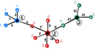
Figure 2. An example of a Stanley tree of type $(3,5,3)$. The circled numbers indicate the labels of the black vertices. The black numbers indicate the labels of the edges. The colors (blue for $1$, red for $2$, green for $3$) indicate the values of the function $f$ on white vertices.

Let $T$ be a bicolored plane tree, i.e., a plane tree with each vertex painted black or white and with edges connecting the vertices of opposite colors. We assume that the tree has $k$ edges labeled with the numbers $1,\dots,k$. We also assume that it has $n$ black vertices labeled with the numbers $1,\dots,n$. The white vertices are not labeled. Being a plane tree means that the set of edges surrounding any given vertex is equipped with a cyclic order related to visiting the edges in the counterclockwise order. In our context the structure of the plane tree can be encoded by a pair of permutations $(\sigma_{1},\sigma_{2})$ with $\sigma_{1},\sigma_{2}\in\mathfrak{S}_{k}$ such that the cycles of $\sigma_{1}$ (respectively, the cycles of $\sigma_{2}$) correspond to labels of the edges surrounding white (respectively, black) vertices. We define the function $f$ that to each white vertex associates the maximum of the labels of its black neighbors. We will say that $T$ is a Stanley tree of type

$$(b_{1},\dots,b_{n})\mathrel{\mathop{\ordinarycolon}}=\Big{(}\big{|}f^{-1}(1)\big{|},\dots,\big{|}f^{-1}(n)\big{|}\Big{)};$$

in other words the type gives the information about the number of the white vertices for which the function $f$ takes a specified value. Figure 2 gives an example of a Stanley tree of type $(3,5,3)$.

Since for a tree the total number of the black and the white vertices is equal to the number of the edges plus $1$, it follows that

(2) $$b_{1}+\cdots+b_{n}+n=k+1.$$

Note that the definition of a Stanley tree of a given type depends implicitly on the value of $k$; in the following we will always assume that $k$ is given by (2).

By $\mathcal{T}_{b_{1},\dots,b_{n}}$ we denote the set of Stanley trees of a specific type $(b_{1},\dots,b_{n})$.

1.3. Coefficients of the top-degree $\mathbf{p}$-square-free monomials

It turns out that in the analysis of the Stanley polynomials it is enough to restrict attention to the $\mathbf{p}$-square-free monomials, i.e., the monomials of the form

(3) $$p_{1}\cdots p_{n}q_{1}^{b_{1}}\cdots q_{n}^{b_{n}}$$

with integers $b_{1},\dots,b_{n}\geq 0$; see [DFŚ10, Section 4] and [Śni16] for a short overview. The following lemma is a reformulation of a result of Rattan [Rat08]; it gives a combinatorial interpretation to the coefficients standing at these $\mathbf{p}$-square-free monomials that are of top-degree in the special case of the Stanley polynomials $\operatorname{Ch}_{k}$ that correspond to a partition with a single part.

Lemma 1.1.

For all integers $b_{1},\dots,b_{n}\geq 0$ such that

(4) $$b_{1}+\cdots+b_{n}+n=k+1$$

the $\mathbf{p}$-square-free coefficient of the Stanley character polynomial is given by

(5) $$\left[p_{1}\cdots p_{n}q_{1}^{b_{1}}\cdots q_{n}^{b_{n}}\right]\operatorname{Ch}_{k}\big{(}\mathbf{p}\times\mathbf{q}\big{)}=\pm\frac{1}{(k-1)!}\left|\mathcal{T}_{b_{1},\dots,b_{n}}\right|.$$

In order to be concise we will not discuss the sign on the right-hand side. The above lemma is a special case of a general formula conjectured by Stanley [Sta06, Conjecture 3] and proved by Féray [Fér10] and therefore we refer to it as the Stanley–Féray character formula. This general formula is applicable also when the assumption (4) is not fulfilled; in this case on the right-hand side of (5) the Stanley trees should be replaced by unicellular maps with some additional decorations; see Section 1.6.1 for more details.

There is another way of calculating the coefficient on the left-hand side of (5); we shall review it in the following. The homogeneous part of degree $k+1$ of the multivariate polynomial $\operatorname{Ch}_{k}\big{(}\mathbf{p}\times\mathbf{q}\big{)}$ (i.e., its homogeneous part of the top degree) is called the free cumulant and is denoted by $R_{k+1}\big{(}\mathbf{p}\times\mathbf{q}\big{)}$.

Example 2.

We continue with the notations from Example 1; it follows that

$$R_{2} =p_{1}q_{1}+p_{2}q_{2},$$

$$R_{3} =-p_{1}^{2}q_{1}+p_{1}q_{1}^{2}-2p_{1}p_{2}q_{2}-p_{2}^{2}q_{2}+p_{2}q_{2}^{2},$$

$$R_{4} =p_{1}^{3}q_{1}-3p_{1}^{2}q_{1}^{2}+3p_{1}^{2}p_{2}q_{2}+p_{1}q_{1}^{3}-3p_{1}q_{1}p_{2}q_{2}+3p_{1}p_{2}^{2}q_{2}$$

$$-3p_{1}p_{2}q_{2}^{2}+p_{2}^{3}q_{2}-3p_{2}^{2}q_{2}^{2}+p_{2}q_{2}^{3},$$

$$R_{5} =-p_{1}^{4}q_{1}+6p_{1}^{3}q_{1}^{2}-4p_{1}^{3}p_{2}q_{2}-6p_{1}^{2}q_{1}^{3}+12p_{1}^{2}q_{1}p_{2}q_{2}-6p_{1}^{2}p_{2}^{2}q_{2}$$

$$+6p_{1}^{2}p_{2}q_{2}^{2}+p_{1}q_{1}^{4}-4p_{1}q_{1}^{2}p_{2}q_{2}+4p_{1}q_{1}p_{2}^{2}q_{2}-4p_{1}q_{1}p_{2}q_{2}^{2}-4p_{1}p_{2}^{3}q_{2}$$

$$+14p_{1}p_{2}^{2}q_{2}^{2}-4p_{1}p_{2}q_{2}^{3}-p_{2}^{4}q_{2}+6p_{2}^{3}q_{2}^{2}-6p_{2}^{2}q_{2}^{3}+p_{2}q_{2}^{4}.$$

Free cumulants were first defined in the context of Voiculescu’s free probability theory and the random matrix theory (see [DFŚ10, Sections 1.3 and 3.4] for references); in the context of the representation theory of the symmetric groups they were introduced in the fundamental work of Biane [Bia98]. From the defining property of the free cumulant it follows that

(6) $$\left[p_{1}\cdots p_{n}q_{1}^{b_{1}}\cdots q_{n}^{b_{n}}\right]\operatorname{Ch}_{k}\big{(}\mathbf{p}\times\mathbf{q}\big{)}=\left[p_{1}\cdots p_{n}q_{1}^{b_{1}}\cdots q_{n}^{b_{n}}\right]R_{k+1}\big{(}\mathbf{p}\times\mathbf{q}\big{)},$$

provided that (4) holds true.

Dołęga, Féray and the second named author [DFŚ10, Section 3.2] introduced another convenient family $S_{2},S_{3},\dots$ of functions on the set of Young diagrams that has the property that for any strictly positive exponents $b_{1},\dots,b_{n}\geq 1$ the coefficient of the corresponding $\mathbf{p}$-square-free monomial (3) in any finite product

$$S_{2}^{\alpha_{2}}S_{3}^{\alpha_{3}}\cdots=\left[S_{2}\big{(}\mathbf{p}\times\mathbf{q}\big{)}\right]^{\alpha_{2}}\left[S_{3}\big{(}\mathbf{p}\times\mathbf{q}\big{)}\right]^{\alpha_{3}}\cdots$$

(for any sequence of integers $\alpha_{2},\alpha_{3},\ldots\geq 0$ such that only finitely many of its entries are non-zero) takes a particularly simple form, cf. [DFŚ10, Theorem 4.2]. On the other hand, the free cumulant $R_{k+1}$ can be written as an explicit polynomial in the functions $S_{2},S_{3},\dots$, cf. [DFŚ10, Proposition 2.2]. By combining these two results it follows that for any strictly positive integers $b_{1},\dots,b_{n}\geq 1$ such that (4) holds true, the right-hand side of (6) is equal to

(7) $$\left[p_{1}\cdots p_{n}q_{1}^{b_{1}}\cdots q_{n}^{b_{n}}\right]R_{k+1}\big{(}\mathbf{p}\times\mathbf{q}\big{)}=(-k)^{n-1}.$$

An astute reader may verify that this result indeed holds true for the data from Example 2, and also that the assumption that $b_{1},\dots,b_{n}$ are strictly positive cannot be weakened.

By combining Equations (5)–(7) we obtain the following result.

Corollary 1.2.

For any strictly positive integers $b_{1},\dots,b_{n}\geq 1$ such that (4) holds true, the number of the Stanley trees of type $(b_{1},\dots,b_{n})$ is equal to

(8) $$\left|\mathcal{T}_{b_{1},\dots,b_{n}}\right|=(k-1)!\ k^{n-1}.$$

Remark 1.3.

If some of the entries of the sequence $b_{1},\dots,b_{n}$ are equal to zero then the number of the Stanley trees of type $(b_{1},\dots,b_{n})$ takes a more complicated form that can be extracted by an application of [DFŚ10, Lemma 4.5].

1.4. The main result: a bijective proof

The above sketch of the proof of Corollary 1.2 has a disadvantage of being purely algebraic. The main result of the current paper (see 2.1 below) is its new, bijective proof. We are not aware of previous bijective proofs of this result in the literature.

Clearly, the right-hand side of (8) can be interpreted as the cardinality of some very simple combinatorial sets, such as the Cartesian product of the set of long cycles in the symmetric group $\mathfrak{S}_{k}$ with the Cartesian power $\{1,\dots,k\}^{n-1}$. We are not aware of a direct bijection between $\mathcal{T}_{b_{1},\dots,b_{n}}$ and some Cartesian product of this flavor. Also, and more importantly, such Cartesian products do not generalize well to the context of the maps with higher genus, which will be discussed in Section 1.6.

For these reasons, as the first step towards the bijective proof we will look for another natural class of combinatorial objects the cardinality of which is given by the right-hand side of (8).

1.5. Minimal factorizations of long cycles

We fix an integer $k\geq 1$ and denote by $\mathfrak{S}_{k}$ the corresponding symmetric group. For a permutation $\pi\in\mathfrak{S}_{k}$ we define its norm $\|\pi\|$ as the minimal number of factors necessary to write $\pi$ as the product of transpositions. (The name length is more common in the literature, but it is confusing in the context of the phrase cycle of a given length; see below.) We say that a permutation $\pi\in\mathfrak{S}_{k}$ is a cycle of length $\ell$ if it is of the form $\pi=(x_{1},\dots,x_{\ell})$. One can prove that in this case the norm of the cycle $\|\pi\|=\ell-1$ is equal to its length less $1$.

Let $a_{1},\dots,a_{n}\geq 2$ be integers. We say that a tuple $(\sigma_{1},\dots,\sigma_{n})$ is a factorization of a long cycle of type $(a_{1},\dots,a_{n})$ if $\sigma_{1},\dots,\sigma_{n}\in\mathfrak{S}_{k}$ are such that the product $\sigma_{1}\cdots\sigma_{n}$ is a cycle of length $k$ and $\sigma_{i}$ is a cycle of length $a_{i}$ for each choice of $i\in\{1,\dots,n\}$.

By the triangle inequality,

$$\sum_{i=1}^{n}(a_{i}-1)=\sum_{i=1}^{n}\|\sigma_{i}\|\geq\|\sigma_{1}\cdots\sigma_{n}\|=k-1.$$

In the current paper we concentrate on minimal factorizations, which correspond to the special case when the above inequality becomes saturated and

(9) $$\sum_{i=1}^{n}(a_{i}-1)=k-1.$$

By $\mathcal{C}_{a_{1},\dots,a_{n}}$ we denote the set of such minimal factorizations of a long cycle of type $(a_{1},\dots,a_{n})$. The name minimal factorization is motivated by the special case when the lengths $a_{1}=\cdots=a_{n}=2$ are all equal to $2$ and hence $\pi=\sigma_{1}\cdots\sigma_{n}$ is a factorization into a product of transpositions; then (9) is satisfied if and only if $n$, the number of factors, takes the smallest possible value.

Biane [Bia96] extended the previous result of Dénes [Dén59] and proved that the number of minimal factorizations $\sigma=\sigma_{1}\dots\sigma_{n}$ of a fixed cycle $\sigma$ of length $k$ into a product of cycles of lengths $a_{1},\dots,a_{n}\geq 2$ for which (9) is fulfilled is equal to $k^{n-1}$. Since in the symmetric group $\mathfrak{S}_{k}$ there are $(k-1)!$ such cycles $\sigma$ of length $k$, it follows that the total number of the minimal factorizations of a long cycle of type $(a_{1},\dots,a_{n})$ is equal to

(10) $$\left|\mathcal{C}_{a_{1},\dots,a_{n}}\right|=(k-1)!\ k^{n-1}$$

and therefore coincides with the right-hand side of (8). Our new proof of Corollary 1.2 will be based on an explicit bijection between the set $\mathcal{T}_{b_{1},\dots,b_{n}}$ of Stanley trees of some specified type and the set $\mathcal{C}_{a_{1},\dots,a_{n}}$ of minimal factorizations of a long cycle of some specified type; see 2.1 for more details.

As a side remark we note that the bijective proof of (10) provided by Biane [Bia96] can be used to construct an explicit bijection between $\mathcal{C}_{a_{1},\dots,a_{n}}$ and the Cartesian product that we mentioned in Section 1.4. By combining Biane’s bijection with the one provided by 2.1 one could get a (very complicated) bijection between $\mathcal{T}_{b_{1},\dots,b_{n}}$ and the Cartesian product from Section 1.4.

1.6. Outlook: permutations, plane trees, maps

For simplicity, in the current paper we consider only the first-order asymptotics of the character (1) of the symmetric group on a cycle $\pi=(k)$, which corresponds to the coefficients of the Stanley polynomial (5) appearing at the top-degree monomials (4). In the light of the aforementioned open problems that concern the fine structure of the symmetric group characters $\operatorname{Ch}_{k}$ evaluated on a cycle (see [GR07, Conjecture 2.4] and [Las08]) it would be interesting to extend the results of the current paper to the coefficients of general $\mathbf{p}$-square-free monomials of the Stanley character polynomial. We will keep this wider perspective in mind in what follows.

Each of the two sets $\mathcal{T}_{b_{1},\dots,b_{n}}$ and $\mathcal{C}_{a_{1},\dots,a_{n}}$ that appear in our main bijection has an algebraic facet and a geometric facet. In the following we will revisit the links between these facets. These geometric facets will be essential for the bijection that is the main result of the current paper.

1.6.1. Stanley trees, revisited

The general form of the Stanley–Féray character formula (see [Sta06, Conjecture 3] and Féray [Fér10]) gives an explicit combinatorial interpretation to the coefficient of an arbitrary monomial in the Stanley polynomial $\operatorname{Ch}_{k}\big{(}\mathbf{p}\times\mathbf{q}\big{)}$, nevertheless it seems that in applications only $\mathbf{p}$-square-free monomials are really useful; see [DFŚ10, Section 4] and [Śni16]. It turns out that in general the coefficient

(11) $$\left[p_{1}\cdots p_{n}q_{1}^{b_{1}}\cdots q_{n}^{b_{n}}\right]\operatorname{Ch}_{k}\big{(}\mathbf{p}\times\mathbf{q}\big{)}$$

is equal (up to the $\pm$ sign) to the number of triples $(\sigma_{1},\sigma_{2},f_{2})$ such that:

• $\sigma_{1},\sigma_{2}\in\mathfrak{S}_{k}$ are permutations with the property that their product

  $$\sigma_{1}\sigma_{2}=(1,2,\dots,k)$$

  is a specific cycle of length $k$;

• $f_{2}$ is a bijection between the set of cycles of the permutation $\sigma_{2}$ and the set $\{1,\dots,n\}$ (we can think that $f_{2}$ is a labeling of the cycles of $\sigma_{2}$);

• we define the function $f_{1}$ on the set of cycles of the permutation $\sigma_{1}$ by setting

  $$f_{1}(c_{1})=\max\big{\{}f_{2}(c_{2})\mathrel{\mathop{\ordinarycolon}}\text{$c_{2}$ is a cycle of $\sigma_{2}$}\\ \text{such that the cycles $c_{1}$ and $c_{2}$ are \emph{not} disjoint}\big{\}}\quad\text{if $c_{1}$ is a cycle of $\sigma_{1}$;}$$

  we require that for each $i\in\{1,\dots,n\}$ the cardinality of its preimage is given by the appropriate exponent of the variable $q_{i}$ in the monomial:

  $$\big{|}f_{1}^{-1}(i)\big{|}=b_{i}.$$

To this algebraic object $(\sigma_{1},\sigma_{2},f_{2})$ one can associate a geometric counterpart, namely a bicolored map. More specifically, it is a graph drawn on an oriented surface with the edges labeled with the elements of the set $\{1,\dots,k\}$. Each white vertex (respectively, each black vertex) corresponds to some cycle of the permutation $\sigma_{1}$ (respectively, to some cycle of the permutation $\sigma_{2}$) so that the counterclockwise cyclic order of the edges around the vertex coincides with the cyclic order of the elements of the set $\{1,\dots,k\}$ that are permuted by the cycle; see [Śni13, Section 6.4].

We assume that the surface on which the graph is drawn is minimal, i.e., after cutting the surface along the edges, each connected component is homeomorphic to a disc; we call such connected components faces of the map. The product $\sigma_{1}\sigma_{2}=(1,2,\dots,k)$ consists of a single cycle which geometrically means that our map has exactly one face; in other words it is unicellular.

The bijection $f_{2}$ geometrically means that the black vertices of our map are labeled by the elements of the set $\{1,\dots,n\}$. Using such a geometric viewpoint, $f_{1}$ becomes a function on the set of white vertices that to a given white vertex associates the maximum of the labels (given by $f_{2}$) of its neighboring black vertices.

By counting the white and the black vertices it follows that the total number of the vertices is equal to

$$b_{1}+\cdots+b_{n}+n.$$

A simple argument based on the Euler characteristic shows that for a unicellular map this number of vertices is bounded from above by $k+1$ (which is the number of the edges plus one) and the inequality becomes saturated (i.e., the equality (4) holds true) if and only if the surface has genus zero, i.e., it is homeomorphic to a sphere.

In the following we consider the case when (4) indeed holds true. It is conceptually simpler to consider such a map drawn on the sphere as drawn on the plane; being unicellular corresponds to the map being a tree. It follows that in this case the geometric object associated above to the triple $(\sigma_{1},\sigma_{2},f_{2})$ that contributes to the coefficient (11) coincides with the Stanley tree of type $(b_{1},\dots,b_{n})$.

The above discussion motivates the notion of the Stanley trees and shows which more general geometric objects should be investigated in order to study more refined asymptotics of the characters of the symmetric groups.

1.6.2. Minimal factorizations

The geometric object that can be associated to a minimal factorization $\sigma_{1},\dots,\sigma_{n}\in\mathfrak{S}_{k}$ of a long cycle of type $(a_{1},\dots,a_{n})$ is a graph with $k$ white vertices (labeled with the elements of the set $\{1,\dots,k\}$) and $n$ black vertices (labeled with the elements of the set $\{1,\dots,n\}$). We connect the black vertex $i$ with the white vertices $\sigma_{i,1},\dots,\sigma_{i,a_{i}}$ that correspond to the elements of the cycle $\sigma_{i}=(\sigma_{i,1},\dots,\sigma_{i,a_{i}})$. This graph is clearly connected, it has $k+n$ vertices and it has $a_{1}+\cdots+a_{n}$ edges; from the minimality assumption (9) it follows that the graph is, in fact, a tree. We may encode the cycles $\sigma_{1},\dots,\sigma_{n}$ by drawing the tree on the plane in such a way that the counterclockwise order of the white vertices surrounding a given black vertex $i$ corresponds to the cycle $\sigma_{i}$; see Figure 3 for an example. On the other hand, we have a freedom of choosing the cyclic order of the edges around the white vertices. In this way a minimal factorization of a long cycle can be encoded (in a non-unique way) by a plane tree with labeled white vertices and labeled black vertices. Later on we will remove this ambiguity by choosing the cyclic order around the white vertices in some canonical way.

Figure 3. One of the plane trees that correspond to the minimal factorization $\sigma_{1}\cdots\sigma_{n}=\sigma_{1}\sigma_{2}\sigma_{3}\sigma_{4}=(1,2,\dots,10)\in\mathfrak{S}_{k}$ of a long cycle with $\sigma_{1}=(7,8,9,10)$, $\sigma_{2}=(1,2)$, $\sigma_{3}=(2,5,6,10)$, $\sigma_{4}=(2,3,4)$, $k=10$ and $n=4$. The black vertices correspond to the cycles $\sigma_{1},\dots,\sigma_{4}$. The white vertices correspond to the elements of the set $\{1,\dots,10\}$ on which acts the symmetric group $\mathfrak{S}_{10}$. The cyclic order of the edges around the black vertices is determined by the cycles $\sigma_{1},\dots,\sigma_{4}$. The cyclic order of the edges around the white vertices is arbitrary.

The original permutation $\sigma_{i}$ can be recovered from the tree by reading the counterclockwise cyclic order of the labels of the neighbors surrounding the black vertex $i$; see Figure 3.

1.7. Overview of the paper

In Section 2 we state our main result (2.1) about existence of a bijection between certain sets of minimal factorizations and Stanley trees; the bijection itself is constructed in Sections 2.1, 2.2, 2.5 and 2.7. It is quite surprising that a bare-boned description of the bijection (without the proof of its correctness) is quite short, nevertheless this algorithm creates a quite complex dynamics, as can be seen by the length of the description of the inverse map. Additionally, in Sections 2.6 and 2.8 we prove that this algorithm is well defined.

As the first step towards the proof of 2.1, in Section 3 we show 3.2, which states that the output of our algorithm indeed is a Stanley tree of a specific type.

Section 4 contains an alternative description of the bijection.

In Section 5 we construct the inverse map.

Finally, in Section 6 we complete the proof of 2.1.

2. The main result: bijection between Stanley trees
and minimal factorizations of long cycles

The following is the main result of the current paper.

Theorem 2.1.

Let $n\geq 2$ and $b_{1},\dots,b_{n}\geq 1$ be integers. We define the integers $a_{1},\dots,a_{n}$ by

(12) $$a_{i}=\begin{cases}b_{i}+1&\text{if }i\in\{1,n\},\\ b_{i}+2&\text{otherwise}.\end{cases}$$

Then the algorithm $\mathcal{A}$ presented below gives a bijection between the set $\mathcal{C}_{a_{1},\dots,a_{n}}$ of minimal factorizations (see Section 1.5) and the set $\mathcal{T}_{b_{1},\dots,b_{n}}$ of Stanley trees (see Section 1.2).

Note that both the notion of a Stanley tree as well as the notion of the minimal factorization implicitly depend on the value of $k$ given, respectively, by (2) and (9). In our context, when (12) holds true, these two values of $k$ coincide.

2.1. The first step of the algorithm $\mathcal{A}$: from a factorization to a tree with repeated edge labels

In the first step of our algorithm $\mathcal{A}$ to a given minimal factorization $(\sigma_{1},\dots,\sigma_{n})\in\mathcal{C}_{a_{1},\dots,a_{n}}$ we will associate a bicolored plane tree $T_{1}$ with labeled black vertices and labeled edges. The remaining part of the current section is devoted to the details of this construction.

2.1.1. The tree $T_{0}$

Just like in Section 1.6.2 we start by creating a graph $T_{0}$ with $n$ black vertices labeled $1,\dots,n$ and with $k$ white vertices labeled $1,\dots,k$, where $k$ is given by (9). Each black vertex $i$ corresponds to the cycle $\sigma_{i}=(\sigma_{i,1},\dots,\sigma_{i,a_{i}})$ and so we connect the black vertex $i$ with the white vertices $\sigma_{i,1},\dots,\sigma_{i,a_{i}}$. By the same argument as in Section 1.6.2 this graph is, in fact, a tree.

In order to give this tree the structure of a plane tree we need to specify the cyclic order of the edges around each vertex. Just like in Section 1.6.2 we declare that going counterclockwise around the black vertex $i$ the cyclic order of the labels of the white neighbors should correspond to the cyclic order $\sigma_{i,1},\dots,\sigma_{i,a_{i}}$. The cyclic order around the white vertices is more involved and we present it in the following.

The path between the two black vertices with the labels $1$ and $n$ will be called the spine; on Figure 5a it is drawn as the horizontal red path. There will be two separate rules that determine the cyclic order of the edges around a given white vertex, depending whether the vertex belongs to the spine or not.

For each white vertex that is not on the spine we declare that going counterclockwise around it, the labels of its black neighbors should be arranged in the increasing way (for example, the neighbors of the white vertex $6$ on Figure 5a listed in the counterclockwise order are $3,4,6$).

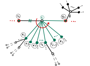
Figure 4. The structure of a white spine vertex $c$ in the plane tree $T_{0}$. The labels of the black spine vertices $\alpha_{c},y_{1}\in\{1,\dots,n\}$ fulfill $\alpha_{c}<y_{1}$. There are $l\geq 0$ non-spine neighbors of the vertex $c$, denoted $x_{1},\dots,x_{l}$. They are all placed (in the counterclockwise cyclic order) after $\alpha_{c}$ and before $y_{1}$. It may happen that $l=0$ and there are no non-spine neighbors of $c$. For the details see Section 2.1.1.

For each white vertex $c$ that belongs to the spine there are exactly two black neighbors that belong to the spine; we denote their labels by $\alpha_{c}$ and $y_{1}$ with $\alpha_{c}<y_{1}$; see Figure 4. Going counterclockwise around $c$, all non-spine edges should be inserted after $\alpha_{c}$ and before $y_{1}$. Their order is determined by the requirement that—after neglecting the vertex $y_{1}$—the cyclic counterclockwise order of the remaining vertices should be increasing. For example, for the white vertex $1$ on Figure 5a we have $\alpha_{1}=7$, $y_{1}=11$ and the counterclockwise cyclic order of the non-$y_{1}$ black neighbors is $4,7,13$.

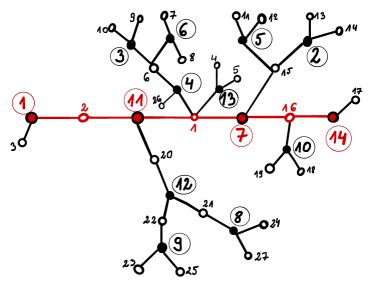
(a)

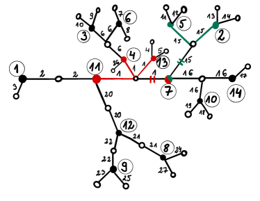
(b)

Figure 5. LABEL:sub@subfig:ex1 The output $T_{0}$ of the first step of the algorithm $\mathcal{A}$ applied to the minimal factorization (13). The spine is the horizontal red path between the vertices $1$ and $14$. LABEL:sub@subfig:ex2 The tree $T_{1}$ with some sample clusters highlighted. The red color indicates the cluster $1$, while the green indicates the cluster $15$. The double transverse lines identify the roots of the respective clusters.

For example, Figure 5a gives the tree $T_{0}$ that corresponds to

$$n=14,\quad k=27,\qquad a_{1}=a_{14}=2,\quad a_{2}=\cdots=a_{13}=3$$

and the minimal factorization $(\sigma_{1},\dots,\sigma_{14})\in\mathcal{C}_{2,3^{12},2}$

(13) $$\sigma_{1}=(2,3),\quad\sigma_{2}=(13,15,14),\quad\sigma_{3}=(6,9,10),\quad\sigma_{4}=(1,6,26),\\ \sigma_{5}=(11,15,12),\quad\sigma_{6}=(6,8,7),\quad\sigma_{7}=(1,16,15)\quad\sigma_{8}=(21,27,24),\\ \sigma_{9}=(22,23,25),\quad\sigma_{10}=(16,19,18),\quad\sigma_{11}=(2,20,1),\\ \sigma_{12}=(20,22,21),\quad\sigma_{13}=(1,5,4),\quad\sigma_{14}=(16,17).$$

We denote by $T_{1}$ the tree $T_{0}$ in which each edge is labeled by its white endpoint and then all labels of the white vertices are removed; see Figures 5b and 6. The tree $T_{1}$ is the output of the first step of the algorithm $\mathcal{A}$.

2.1.2. Information about the initial tree $T_{1}$

In the current section we will define certain sets and functions that describe the shape of the initial tree $T_{1}$. In the language of programmers: we will create variables $B_{c}$, $\alpha_{c}$, $\mathcal{B}$, and $\mathfrak{C}$ that will not change their values during the execution of the algorithm $\mathcal{A}$.

For $c\in\{1,\dots,k\}$ by the cluster $c$ we mean the set of edges that carry the label $c$, together with their black endpoints. We will also say that $c$ is the label of this cluster. All edges in a given cluster have the same white endpoint; this property will be preserved by the action of our algorithm. This common white vertex will be called the center of the cluster. For example, in Figure 5b the cluster $1$ is drawn in red, while the cluster $15$ is drawn in green. We denote by $B_{c}\subseteq\{1,\dots,n\}$ the set of labels of the black vertices in the cluster $c$ in the tree $T_{1}$.

Each cluster may contain either zero, one, or two black spine vertices. A cluster is called a spine cluster if it contains exactly two black spine vertices. The set of labels of such spine clusters will be denoted by $\mathfrak{C}\subseteq\{1,\dots,k\}$.

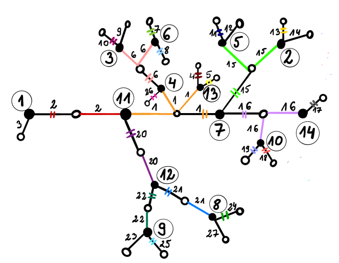
Figure 6. The tree $T_{1}$ that is the starting point of the second step of the algorithm $\mathcal{A}$ for the minimal factorization (13). Essentially this is an enlarged version of Figure 5b with some additional highlights. For the sake of clarity we paint the non-root edges of each cluster in one color, while the root edge is marked with two transverse lines of the same color.

We orient the non-spine edges of the tree so that the arrows point towards the spine. The root of a non-spine cluster is defined as the unique edge outgoing from the center. The root of a spine cluster is defined as the edge with the smallest label of the black endpoint among the two spine edges in the cluster; with the notations of Figure 4 it is the edge between the vertices $c$ and $\alpha_{c}$. For example, in Figure 6 the root of a cluster is marked with two transverse lines. Heuristically, our strategy will be to keep removing the edges from the cluster; the root is the unique cluster edge that will remain at the end. The notion of the root will not be used in the description of the algorithm $\mathcal{A}$, nevertheless it will be a convenient tool for proving later its correctness.

The black end of the root of a cluster $c\in\{1,\dots,k\}$ in the tree $T_{1}$ will be called the anchor of the cluster $c$. Its label will be denoted by $\alpha_{c}\in\{1,\dots,n\}$. By definition, the label of the anchor will not change during the execution of the algorithm. However, it may happen at later steps that the anchor (i.e., the black vertex that carries the label $\alpha_{c}$) is no longer one of the endpoints of the root. When it does not lead to confusions we will identify the anchor (understood as a black vertex) with its label $\alpha_{c}$.

By $\mathcal{B}\subseteq\{1,\dots,n\}$ we denote the set of the labels of black spine vertices.

A cluster is called a leaf if it contains exactly one edge. For example, in Figures 5b and 6 the cluster $10$ is a leaf.

For the example from Figures 5b and 6 we have:

(14) $$\mathcal{B}=\{1,7,11,14\},\quad\mathfrak{C}=\{1,2,16\},\\ B_{1}=\{4,7,11,13\},\quad B_{2}=\{1,11\},\quad B_{6}=\{3,4,6\},\quad B_{15}=\{2,5,7\},\\ B_{16}=\{7,10,14\},\quad B_{20}=\{11,12\},\quad B_{21}=\{8,12\},\quad B_{22}=\{9,12\},\\ \alpha_{1}=7,\quad\alpha_{2}=1,\quad\alpha_{6}=4,\quad\alpha_{15}=7,\\ \alpha_{16}=7,\quad\alpha_{20}=11,\quad\alpha_{21}=12,\quad\alpha_{22}=12.$$

We did not list the values of $B_{i}$ and $\alpha_{i}$ for white vertices $i$ that are non-spine leaves because these values will not be used by our algorithm.

Recall that we orient the non-spine edges of the tree so that the arrows point towards the spine. The set of non-spine clusters is partially ordered by the orientations of the edges as follows: a cluster $c_{1}$ is a predecessor of a cluster $c_{2}$ if the path from the spine to the center of the cluster $c_{2}$ passes through the center of the cluster $c_{1}$. This partial order can be extended to a linear order (not necessarily in a unique way). Let $\Sigma$ be the sequence of the clusters that are non-spine and non-leaf, arranged according to this linear order. For example, for the tree $T_{1}$ shown on Figure 5a we can choose $\Sigma=(6,15,20,21,22)$.

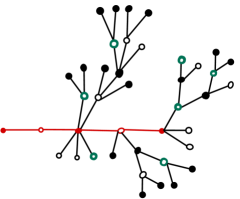
Figure 7. The tree $T_{1}$ shown without the labels. The red edges indicate the spine. The thick green empty circles indicate white leftist vertices.

The aforementioned orientations of the edges allow us also to use some vocabulary taken from the theory of rooted trees, at least for the vertices which are away from the spine. For example, the parent of a non-spine vertex $v$ is the unique vertex $w$ such that there is an oriented edge from $v$ to $w$. The terms such as children and descendants of a non-spine vertex are defined accordingly.

Let $c_{1},c_{2}$ be clusters in the tree $T_{1}$ and let $v_{1},v_{2}$ be their centers. We say that the cluster $c_{2}$ is a child of the cluster $c_{1}$ or, in other words, the cluster $c_{1}$ is the parent of the cluster $c_{2}$ if there exists a black vertex $w$ that is a child of the vertex $v_{1}$ and such that $v_{2}$ is a child of $w$, i.e., $v_{2}$ is a grandchild of $v_{1}$.

In the plane tree $T_{1}$ we can split the set of white non-spine vertices into the set of leftist vertices and the set of non-leftist vertices. A white non-spine vertex is called leftist in the tree $T_{1}$ if it is a leftmost child of its parent when viewed from the point of view of the parent. Note that a black spine vertex may have two leftmost children located on either side of the spine. For example, for the tree $T_{1}$ shown on Figure 7, the white leftist vertices are drawn as thick green empty circles. We say that a cluster in $T_{1}$ is leftist if its center is a leftist vertex.

2.2. The second step of the algorithm $\mathcal{A}$: from a tree with repeated edge labels to a tree with unique edge labels

The starting point of the second step of our algorithm $\mathcal{A}$ is the bicolored plane tree $T_{1}$ with black vertices labeled $1,\dots,n$ and with edges labeled with the numbers $1,\dots,k$; note that the edge labels are repeated. Our goal in this second step of the algorithm is to transform the tree so that the edge labels are not repeated.

We declare that at the beginning all clusters of the tree $T_{1}$ are untouched. Also, each non-spine black vertex is declared to be untouched. On the other hand, each black spine vertex is declared to be touched.

The second step of the algorithm will consist of two parts: firstly we apply the spine treatment (Section 2.5), then we apply the rib treatment (Section 2.7). In fact, these two parts are very similar: each of them consists of an external loop that has a nested internal loop; one could merge these two parts and regard them as an instance of a single external loop that treats the spine vertices and the non-spine vertices in a slightly different way.

During the action of the forthcoming algorithm some edges will be removed from each cluster. The root of the cluster may change during the execution of the algorithm. Also, as we already mentioned, the anchor of a cluster may no longer be the black endpoint of the root. On the positive side, the following invariant guarantees that some properties of a cluster will persist (the proof is postponed to 2.5 and 2.7).

Invariant 2.2.

At each step of the algorithm and for each cluster $c$ the following properties hold true:

1. the edges of the cluster $c$ have a common white endpoint (called, as before, the center of the cluster),

2. the anchor of $c$ is a black vertex that is connected by an edge with the center of $c$,

3. the root of $c$ is one of the edges that form the cluster $c$,

4. if the black endpoint of the root of $c$ is not equal to the anchor $\alpha_{c}$ then this black endpoint is touched.

Be advised that distinct clusters may at later stages of the algorithm share the same center.

The algorithm will be described in terms of two operations, called bend and jump; we present them in the following. Each of them decreases the number of the white vertices by $1$, as well as decreases the number of edges by $1$. The edge that disappears has a repeated label, in this way the set of the edge labels remains unchanged.

2.3. The building blocks of the second step: bend $\mathbb{B}_{x,y}$

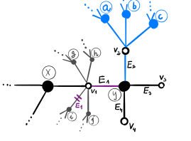
(a)

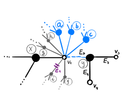
(b)

Figure 8. LABEL:sub@subfig:exA The initial configuration of the tree before the bend operation $\mathbb{B}_{x,y}$ was applied. The vertex $y$ belongs to the cluster $E_{1}$. The center of $E_{1}$ is equal to $v_{1}$. The anchor of $E_{1}$ is equal to $x$. The black endpoint of the root of $E_{1}$ is equal to $i$. We assume that $y\notin\{x,i\}$. The neighbors of $y$, listed in the clockwise order, are: $v_{1},v_{2},\dots,v_{d}$, and the corresponding edges connecting $y$ with the neighbors are: $E_{1},\dots,E_{d}$. For a complete list of notations and assumptions see Section 2.3.1.
LABEL:sub@subfig:exB The output of $\mathbb{B}_{x,y}$. The edge connecting $v_{2}$ with $y$ was rotated counterclockwise so that the vertex $v_{2}$ was merged with $v_{1}$. For a detailed description see Section 2.3.2.

2.3.1. Assumptions about the input of $\mathbb{B}_{x,y}$.

We list below the assumptions about the input of the operation bend. We also introduce some notations.

1. The operation $\mathbb{B}_{x,y}$ takes as an input a bicolored tree $T$ that is assumed to be as in 2.2, together with a choice of two distinct black vertices $x$, $y$. We assume that there is a cluster $E_{1}$ such that $x$ is the anchor of $E_{1}$ and $y$ belongs to $E_{1}$; see Figure 8a. We denote the center of $E_{1}$ by $v_{1}$.

2. We denote by $i$ the black endpoint of the root of the cluster $E_{1}$. We assume that $i\neq y$.

3. We also assume that the black vertex $y$ has degree $d\geq 2$; we denote the edges around the vertex $y$ by $E_{1},\dots,E_{d}$ (going clockwise, starting from the edge $E_{1}$ between $v_{1}$ and $y$). We denote the white endpoint of the edge $E_{i}$ by $v_{i}$.

2.3.2. The output of $\mathbb{B}_{x,y}$

The bend operation can be thought of as a counterclockwise rotation of the edge $E_{2}$ around the vertex $y$ so that it is merged with the edge $E_{1}$; a more formal description of the output of $\mathbb{B}_{x,y}$ is given as follows.

We remove the edge between the vertices $y$ and $v_{2}$. The label of the edge between $v_{1}$ and $y$ is changed to $E_{2}$. If the removed edge was the root of the cluster $E_{2}$, the aforementioned edge between $v_{1}$ and $y$ becomes the new root of the cluster $E_{2}$.

Then we merge the vertex $v_{2}$ with the vertex $v_{1}$ in such a way that going clockwise around $v_{1}$ the newly attached edges are immediately before the edge $E_{2}$ (these edges are marked blue on Figure 8).

From the following on we declare that the cluster $E_{1}$ is touched and also the black vertex $y$ is touched. It is easy to check that the output tree still fulfills the properties from 2.2.

We will say that some operation on the tree separates the root and the anchor in a cluster $c$ if (i) before this operation was applied the anchor of $c$ was the black endpoint of the root of $c$, and (ii) after this operation is performed this is no longer the case. It is easy to check that the following simple lemma holds true.

Lemma 2.3.

The bend operation does not separate the root and the anchor in any cluster.

2.4. The building blocks of the second step: jump $\mathbb{J}_{x,y}$

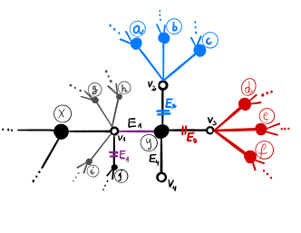
(a)

(b)

Figure 9. LABEL:sub@subfig:jumpA The initial configuration of the tree before the jump operation $\mathbb{J}_{x,y}$ was applied. The black vertex $y$ belong to the cluster $E_{1}$. The center of $E_{1}$ is equal to $v_{1}$, the anchor of this cluster is equal to $x$. The vertex $j$ is the first immediately after $y$ if we visit the neighbors of $v_{1}$ in the clockwise order; we assume that $j$ is the black endpoint of the root of $E_{1}$. The neighbors of $y$ listed in the clockwise order are: $v_{1},v_{2},\dots,v_{d}$. This figure depicts the special case when $j\neq x$. In this case the assumption (I4) applied to the cluster $E_{1}$ guarantees that the vertex $j$ is touched. For the full list of assumptions and notations see Section 2.4.1.
LABEL:sub@subfig:jumpB The output of $\mathbb{J}_{x,y}$. The edges connecting $y$ with $v_{1},v_{2},v_{3}$ were removed. The vertices $v_{2}$ and $v_{3}$ were replaced by a new vertex $w$. The vertex $w$ is connected by new edges to $j$ and $y$. In a typical application, in the initial configuration in the cluster $E_{2}$ the anchor as well as the black endpoint of the root are both equal to $y$; then in the output the anchor of $E_{2}$ is no longer the endpoint of the root. For a detailed description see Section 2.4.2.

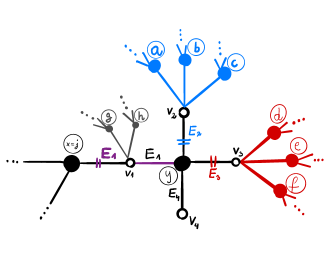
(a)

(b)

Figure 10. LABEL:sub@subfig:scjumpA The initial configuration of the tree before the jump operation $\mathbb{J}_{x,y}$ was applied in the special case when $j=x$. For the notations see the caption of Figure 10. The vertex $x=j$ is assumed to be touched.
LABEL:sub@subfig:scjumpB The output of $\mathbb{J}_{x,y}$ in the special case when $j=x$.

2.4.1. Assumptions about the input of $\mathbb{J}_{x,y}$.

We list below the assumptions about the input of the operation jump. We also introduce some notations.

1. The operation $\mathbb{J}_{x,y}$ takes as an input a bicolored tree $T$ that is assumed to be as in 2.2, together with a choice of two black vertices $x$, $y$. We assume that there is a cluster $E_{1}$ such that $x$ is the anchor of $E_{1}$ and $y$ belongs to $E_{1}$; see Figures 9a and 9a. We denote by $v_{1}$ the center of the cluster $E_{1}$. We also assume that the labels of the vertices $x,y\in\{1,\dots,n\}$ fulfill $x<y$.

2. We denote by $j$ the black neighbor of $v_{1}$ that—going clockwise around the vertex $v_{1}$—is immediately after $y$ (note that it may happen that $j=x$; see Figure 9a). We assume that $j$ is the black endpoint of the root of the cluster $E_{1}$; see Figures 9a and 9a.

3. We also assume that the black vertex $y$ has degree $d\geq 3$; we denote the edges around the vertex $y$ by $E_{1},\dots,E_{d}$ (going clockwise, starting from the edge $E_{1}$). For $i\in\{1,\dots,d\}$ we denote the white endpoint of the edge $E_{i}$ by $v_{i}$.

4. We assume that the vertex $x$ is touched.

2.4.2. The output of $\mathbb{J}_{x,y}$

The output of $\mathbb{J}_{x,y}$ is defined as follows. We remove the three edges connecting $y$ with the three vertices $v_{1},v_{2},v_{3}$. We create a new white vertex denoted $w$; this vertex is said to be artificial; we will use this notion later in the analysis of the algorithm.

We connect $w$ to the vertex $j$ by a new edge that we label $E_{2}$; more specifically, going clockwise around $j$ the newly created edge $E_{2}$ is immediately after the edge $E_{1}$. This newly created edge replaces the removed edge between $y$ and $v_{2}$, so if this removed edge was the root of the cluster $E_{2}$, we declare that the new edge $E_{2}$ becomes now the new root of the cluster $E_{2}$.

We also connect the new vertex $w$ to the vertex $y$ by a new edge that we label $E_{3}$; the position of the edge $E_{3}$ in the vertex $y$ replaces the three edges that were removed from $y$. Again, this newly created edge replaces the removed edge between $y$ and $v_{3}$, so if this removed edge was the root of the cluster $E_{3}$, we declare that the new edge $E_{3}$ becomes now the new root of the cluster $E_{3}$.

We merge the vertices $v_{2}$ and $v_{3}$ with the vertex $w$. More specifically, the clockwise cyclic order of the edges around the vertex $w$ is as follows: the edge $E_{2}$, then the edges from the vertex $V_{3}$ (listed in the clockwise order starting from the removed edge $E_{3}$; on Figures 10 and 10 these edges are marked red), the edge $E_{3}$, then the edges from the vertex $v_{2}$ (listed in the clockwise order starting from the removed edge $E_{2}$; on Figures 10 and 10 these edges are marked blue); see Figures 9b and 9b.

From the following on we declare that the cluster $E_{1}$ is touched and also the black vertex $y$ is touched.

It is easy to check that the following simple lemma holds true.

Lemma 2.4.

The jump operation separates the root and the anchor only in (at most) a single cluster. This potentially exceptional cluster is the one that with the notations of Figures 10 and 10 is denoted by $E_{2}$, and this separation occurs if and only if in the initial configuration both the anchor of $E_{2}$ as well as the black endpoint of the root of $E_{2}$ are equal to $y$.

In fact, we will use the jump operation only in the context when it indeed separates the root and the anchor in $E_{2}$. In this context $E_{2}$ will turn out to be a leftist cluster.

It is easy to check that the output tree still fulfills the properties from 2.2. The only slightly challenging part of the proof concerns verifying that the condition (I4) holds true for the cluster $E_{2}$ if the separation of the root and the anchor occurs. For this purpose we need to show that vertex $j$ is touched. In the case when $j\neq x$ we use the assumption that (I4) for the cluster $E_{1}$ was valid in the initial configuration of the tree and hence $j$ was touched, as required. In the remaining case when $j=x$ we use assumption (J4).

2.5. The spine treatment

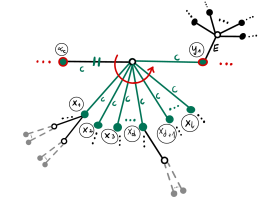
(a)

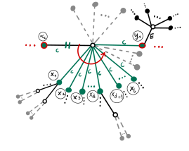
(b)

Figure 11. LABEL:sub@subfig:untouched1 A spine cluster $c$ of the tree $T_{1}$ corresponding to the part of the tree $T_{0}$ on Figure 4. The black vertices $\alpha_{c},y_{1}$ with $\alpha_{c}<y_{1}$ are spine vertices. The vertex $\alpha_{c}$ is the anchor of the cluster $c$ as well as the black endpoint of the root of the cluster $c$. The non-spine vertices in the cluster $c$ are denoted by $x_{1},\dots,x_{l}$ with $l\geq 0$. If $l>0$, we denote by $x_{d}=\min B_{c}\setminus\{\alpha_{c},y_{1}\}$ the vertex with the minimal label among non-spine vertices in the cluster. LABEL:sub@subfig:untouched2 The structure of the cluster $c$ at a later stage of the algorithm as long as it remains untouched. New edges attached to the center of $c$ might have been created on either side of the edge connecting the center with $y_{1}$. See 2.5 (P2) for details.

For each spine cluster $C\in\mathfrak{C}$ we apply the following procedure (the final output will not depend on the order in which we choose the clusters from $\mathfrak{C}$). In the language of programmers we run the external loop (or the main loop) over the variable $C$. Since the spine in the tree $T_{1}$ is a path, the intersection $B_{C}\cap\mathcal{B}$ corresponds to the labels of the two black spine vertices of the cluster $C$ in the tree $T_{1}$. One of these two vertices is the anchor $\alpha_{C}$ of the cluster, we denote the other one by $y_{1}$; in this way $\alpha_{C}<y_{1}$. As we will prove later (see 2.5, property (P2)), at the time of the execution of this particular loop iteration, the spine cluster $C$ is of the form shown on Figure 11b.

We run the following internal loop over the variable $y\in B_{C}\setminus\{\alpha_{C}\}$ (with the ascending order). If $y=y_{1}$ or if the vertex labels $y,\alpha_{C}\in\{1,\dots,n\}$ fulfill $y<\alpha_{C}$ then we apply $\mathbb{B}_{\alpha_{C},y}$; otherwise we apply $\mathbb{J}_{\alpha_{C},y}$.

Example 3.

We continue the example from Figure 5b. We recall that $\mathfrak{C}=\{1,2,16\}$.

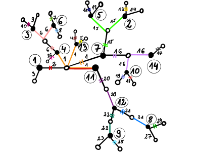
(a)

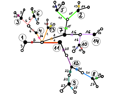
(b)

Figure 12. LABEL:sub@subfig:ex3 The output of $\mathbb{B}_{1,11}$ applied to the tree from Figure 6.
LABEL:sub@subfig:ex4 The output of $\mathbb{B}_{7,4}$ applied to the tree from LABEL:sub@subfig:ex3.

For $C=2$ we recall that $\alpha_{2}=1$ so we have $y_{1}=11$. Since $B_{2}\setminus\{1\}=\{11\}$, the internal loop is applied once with $y=11$. As a result we apply $\mathbb{B}_{1,11}$; see Figure 12a.

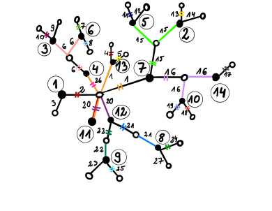
(a)

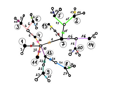
(b)

Figure 13. LABEL:sub@subfig:ex5 The output of $\mathbb{B}_{7,11}$ applied to the tree from Figure 12b.
LABEL:sub@subfig:ex6 The output of $\mathbb{J}_{7,13}$ applied to the tree from LABEL:sub@subfig:ex5.

For $C=1$ we recall that $\alpha_{1}=7$ so we have $y_{1}=11$. Since $B_{1}\setminus\{7\}=\{4,11,13\}$ the internal loop runs over: $\bullet$ $y=4$ and we apply $\mathbb{B}_{7,4}$, see Figure 12b; $\bullet$ $y=11$ and we apply $\mathbb{B}_{7,11}$; see Figure 13a; $\bullet$ $y=13$ and we apply $\mathbb{J}_{7,13}$; see Figure 13b.

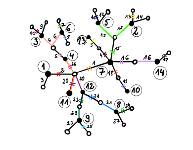
(a)

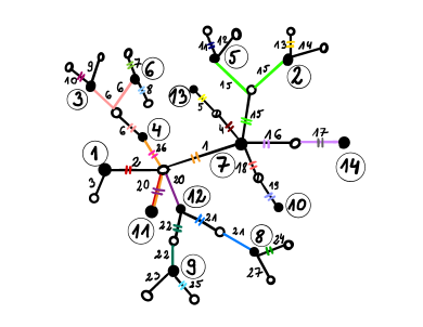
(b)

Figure 14. LABEL:sub@subfig:ex7 The output of $\mathbb{J}_{7,10}$ applied to the tree from Figure 13b. LABEL:sub@subfig:ex8 The output of $\mathbb{B}_{7,14}$ applied to the tree from LABEL:sub@subfig:ex7.

For $C=16$ we recall that $\alpha_{16}=7$ so we have $y_{1}=14$. Since $B_{16}\setminus\{7\}=\{10,14\}$ the internal loop runs over: $\bullet$ $y=10$ and we apply $\mathbb{J}_{7,10}$; see Figure 14a; $\bullet$ $y=14$ and we apply $\mathbb{B}_{7,14}$; see Figure 14b.

2.6. Correctness of the spine treatment algorithm

Before we present the remaining part of the algorithm (in Section 2.7) we will show that the above spine treatment is well-defined in the sense that the assumptions for the bend and jump operations (Sections 2.3.1 and 2.4.1) are indeed fulfilled during the spine treatment. We will show the following stronger result.

Proposition 2.5.

At each step of the spine treatment algorithm, the current value of the tree $T$ fulfills the following properties.

1. The tree $T$ fulfills the properties described in 2.2.

2. Let $c$ be a spine cluster of the initial tree $T_{1}$; we denote by $\alpha_{c},y_{1}$ the black spine vertices in this cluster with $\alpha_{c}<y_{1}$. Assume that the cluster $c$ is still untouched in the tree $T$.

   Then the vertex $\alpha_{c}$ is both the anchor of the cluster $c$ as well as the black endpoint of the root of the cluster $c$.

   Additionally, we compare:

   1. the cyclic order of the black vertex labels of the edges surrounding the center of the cluster $c$ in the original tree $T_{1}$ (i.e. the cyclic order of the black endpoints’ labels of the cluster $c$ in $T_{1}$); see Figure 11a

   with

   1. the cyclic order of the black endpoints’ labels of the edges surrounding the center of the cluster $c$ in the tree $T$; see Figure 11b.

   Then (P2)(ii) is obtained from (P2)(i) by adding some additional vertices that do not belong to the cluster $c$; these additional vertices occur on either side of the edge connecting the center of the cluster $c$ with $y_{1}$; see Figure 11.

3. The set of clusters which are touched coincides with the set of values that the variable $C$ (in the external loop of the spine treatment algorithm) took in the past.

4. For each bend operation (respectively, for each jump operation) performed during the spine treatment algorithm the assumptions (B1)–(B3) (respectively, the assumptions (J1)–(J4)) are fulfilled; in this way each bend/jump operation is well-defined.

Proof.

In the first part of the proof we will show that (B3), (J3) and (J4) are fulfilled in each step of the spine treatment.

Note that during the spine treatment algorithm we perform operations $\mathbb{B}_{x,\cdot}$ and $\mathbb{J}_{x,\cdot}$ for $x\in\mathcal{B}$. From the very beginning each black spine vertex is touched, so the assumption (J4) is fulfilled in each step of the spine treatment.

In order to show (B3) and (J3) we will use the observation that when one of the operations $\mathbb{B}_{\cdot,y}$ or $\mathbb{J}_{\cdot,y}$ is performed, the degree of each black vertex that is different from $y$ increases or remains the same.

Consider some black vertex $y$ of the initial tree $T_{1}$ that does not belong to the spine. In this case the vertex $y$ belongs to at most one spine cluster, so during the spine treatment algorithm we perform at most one operation of the form $\mathbb{B}_{\cdot,y}$ or $\mathbb{J}_{\cdot,y}$. Therefore, the degree of $y$ (at the time when this unique $\mathbb{B}_{\cdot,y}/\mathbb{J}_{\cdot,y}$ operation is performed) is at least its degree in the initial tree $T_{1}$. The latter degree, by construction, is equal to the length of the cycle $\sigma_{y}$ so it is equal to the parameter $a_{y}$ that appears in the statement of 2.1. By (12) we get $a_{y}=b_{y}+2\geq 3$, as required.

Consider now some black vertex $y$ of the initial tree $T_{1}$ that belongs to the spine. In this case the vertex $y$ belongs to at most two spine clusters. It follows that we perform no operations of the form $\mathbb{J}_{\cdot,y}$ at all, and we perform at most two operations of the form $\mathbb{B}_{\cdot,y}$. In the case when we perform a single such an operation $\mathbb{B}_{\cdot,y}$, the assumption (B3) is fulfilled because the degree of $y$ at the time when this operation is performed is at least $a_{y}\geq b_{y}+1\geq 2$, by the same argument as in the previous paragraph. The other case when two such bend operations $\mathbb{B}_{\cdot,y}$ are performed can occur only if $y\notin\{1,n\}$ is not one of the endpoints of the spine; it follows therefore that the initial degree of the vertex $y$ is equal to $a_{y}=b_{y}+2\geq 3$. The bend operation $\mathbb{B}_{\cdot,y}$ decreases the degree of the black vertex $y$ by $1$. Therefore, at the time when the first operation $\mathbb{B}_{\cdot,y}$ performed, the degree of $y$ is at least $a_{y}\geq 3$ while when the second such an operation is performed, the degree $y$ is at least $a_{y}-1\geq 2$, as required. This concludes the proof that the assumptions (B3) and (J3) are fulfilled in each step of the spine treatment algorithm.

In the second part of the proof, in order to show (P1)–(P4) we will use induction over the variable $C$ in the main loop of the spine treatment algorithm. Our inductive assumption is that at the time when the iteration of the main loop starts or ends, the properties (P1)–(P3) are fulfilled.

The induction base. The input tree $T_{1}$ clearly fulfills the conditions (P1)–(P3).

The inductive step. We consider some moment in the action of the spine treatment algorithm when a new iteration of the external loop begins. By the inductive assumption the current value of the tree $T$ fulfills the conditions (P1)–(P3). We denote by $C$ the current value of the variable over which the external loop runs. The assumption (P3) implies that the cluster $C$ is untouched; it follows that the assumption (P2) is applicable to this cluster and hence the cluster $C$ has the form shown on Figure 11b. We denote by $x_{1},\dots,x_{l}$ with $l\geq 0$ the non-spine vertices of the cluster listed in the counterclockwise order, cf. Figure 11. If $l>0$ we denote by $x_{d}=\min B_{C}\setminus\{\alpha_{C},y_{1}\}$ the vertex with the minimal label among non-spine black vertices in this cluster. In the special case when $l=0$ and there are no non-spine vertices in the cluster $c$, the vertex $x_{d}$ is not well-defined and the following analysis requires very minor adjustments.

We will follow the action of the internal loop (over the variable $y$) and we will show that in each step the properties (P1), (P2) and (P4) are fulfilled. A straightforward analysis shows that the variable $y$ in the internal loop will take the following values (listed in the chronological order):

$$\underbrace{x_{d},x_{d+1},\dots,x_{l},}_{\begin{subarray}{c}\text{phase \ref{item:etap1},}\\[3.01389pt] \text{elements that are}\\ \text{ smaller than $\alpha_{C}$}\end{subarray}}\underbrace{x_{1},x_{2},\dots,x_{i},}_{\begin{subarray}{c}\text{phase \ref{item:etap2},}\\[3.01389pt] \text{elements that are}\\ \text{greater than $\alpha_{C}$ and smaller than $y_{1}$}\end{subarray}}\underbrace{y_{1},}_{\text{phase \ref{item:etap3}}}\qquad\underbrace{x_{i+1},\dots,x_{d-1}}_{\begin{subarray}{c}\text{phase \ref{item:etap4},}\\[3.01389pt] \text{elements that are}\\ \text{greater than $y_{1}$}\end{subarray}}$$

(note that in the exceptional case when $d=1$ this list has a slightly different form that also depends whether $x_{1}<\alpha_{C}$ or not), therefore the execution of the internal loop can be split into the following four phases:

1. some number of the bend operations of the form $\mathbb{B}_{\alpha_{C},\cdot}$,

2. some number of jump operations $\mathbb{J}_{\alpha_{C},\cdot}$,

3. one bend operation $\mathbb{B}_{\alpha_{C},y_{1}}$,

4. some more jump operations $\mathbb{J}_{\alpha_{C},\cdot}$.

For proving (P4) note that the conditions (B3), (J3) and (J4) are already proved; thus in order to show that all bend/jump operations are well-defined, it is enough to show (B1) and (B2), respectively (J1) and (J2). In the following we will analyze the phases (I)–(IV) one by one and we will check that it is indeed the case. The evolution of the cluster $C$ over time in these four phases is shown on Figures 11b, 15, 16 and 17 with $c\mathrel{\mathop{\ordinarycolon}}=C$.

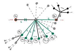
(a)

(b)

Figure 15. LABEL:sub@subfig:untouched3 The structure of the spine cluster $c$ from Figure 11b after performing the first bend operation in the phase (I), namely $\mathbb{B}_{\alpha_{c},x_{d}}$. This figure was obtained from Figure 11b by adding some additional vertices that do not belong to the cluster $c$; going counterclockwise these additional vertices occur after $x_{d}$ and before $x_{d+1}$.
LABEL:sub@subfig:untouched4 The structure of the cluster $c$ after the completion of the phase (I). This figure was obtained from LABEL:sub@subfig:untouched3 by adding some additional vertices that do not belong to the cluster $c$; going counterclockwise these additional vertices occur after $x_{d+i}$ and before $x_{d+i+1}$ for each $i\in\{1,\dots,l-d-1\}$, as well as after $x_{l}$ and before $y_{1}$.

(a)

(b)

Figure 16. LABEL:sub@subfig:untouched5 The structure of the spine cluster $c$ from Figure 15b after performing the first jump operation in the phase (II). This figure was obtained from Figure 15b by removal of the edge $c$ with its black endpoint $x_{1}$ from the center of the cluster $c$ and by combining black $x_{1}$ and $\alpha_{c}$ with a new white vertex.
LABEL:sub@subfig:untouched6 The structure of the cluster $c$ from LABEL:sub@subfig:untouched5 after completion of the phase (II). This figure is obtained from LABEL:sub@subfig:untouched5 by removal of the edge $c$ with its black endpoint $x_{k}$ from the center of the cluster $c$ and by combining black $x_{k}$ and $\alpha_{c}$ with a new white vertex for each $k\in\{2,\dots,i\}$.

We start with the first bend operation from the phase (I), namely $\mathbb{B}_{\alpha_{c},x_{d}}$. (Note that in the exceptional case when $d=1$ and $x_{1}>\alpha_{c}$ the phase (I) is empty and there is nothing to prove.) The assumptions (B1)–(B2) are clearly fulfilled for this first operation; see Figure 11b. Looking at Figure 15a, it is easy to verify that the bend operation preserves the properties from 2.2. We do not modify any other spine clusters, so also the assumption (P2) is preserved for this first bend operation.

It is easy to check that the above arguments remain valid also for the remaining bend operations from the phase (I).

We move on to the first jump operation $\mathbb{J}_{\alpha_{C},x_{1}}$ from the phase (II). The assumptions (J1)–(J2) are clearly fulfilled for this operation $\mathbb{J}_{\alpha_{C},y}$; see Figure 15b. (In the exceptional case if (a) $d=1$ and $x_{1}<\alpha_{C}$, or (b) $y_{1}<x_{1}$ the phase (II) is empty and there is nothing to prove.) We do not modify any other spine clusters, so the assumption (P2) is still fulfilled.

It easy to check that the above arguments remain valid also for the remaining jump operations from the phase (II).

The phase (III) consists of the single bend operation $\mathbb{B}_{\alpha_{C},y_{1}}$, see Figure 16b. Going counterclockwise around $y_{1}$ we denote by $E$ the label of the edge that is immediately after the edge $C$; see Figure 16b. We remind that each bend operation preserves the properties from 2.2. From Figure 17, it is easy to see that if the cluster $E$ is non-spine or spine and touched, then we do not disturb any other untouched spine clusters, so the assumption (P2) is still fulfilled. If $E$ is an untouched spine cluster, then either (a) the vertex $y$ is both the anchor of the cluster $E$ as well as the black endpoint of the root of the cluster $E$, or (b) $y$ is the black spine vertex of the cluster $E$ with the larger label. In both cases, the untouched spine cluster $E$ still fulfills (P2).

Finally, we move on to the phase (IV); the arguments that we used in the phase (II) are also applicable here.

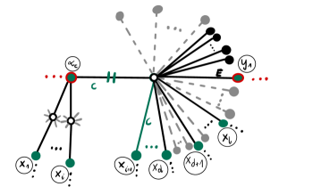
Figure 17. The structure of the cluster $c$ from Figure 16b after performing the phase (III). The Figure 17 is obtained from Figure 16b by adding some additional vertices that do not belong to the cluster $c$; going counterclockwise these additional vertices occur after $y_{1}$.

Note that during the execution of the internal loop we performed only operations of the form $\mathbb{B}_{\alpha_{C},y}$ and $\mathbb{J}_{\alpha_{C},y}$ for $y\in B_{C}$, so we touched exactly one cluster, namely $C$. Therefore, in each step of the internal loop the assumption (P3) is fulfilled. This completes the proof of the inductive step. ∎

2.7. The rib treatment

In the following we will use the word rib as a synonym for non-spine.

In the current section we continue the algorithm from Section 2.5. For each successive cluster $C$ from the sequence $\Sigma$ we apply the following procedure. In the language of programming we execute an external loop over the variable $C$.

We run the following internal loop over the variable $y\in B_{C}\setminus\{\alpha_{c}\}$ (with the ascending order): if $y<\alpha_{c}$ we apply $\mathbb{B}_{\alpha_{c},y}$; otherwise we apply $\mathbb{J}_{\alpha_{c},y}$.

Example 4.

We continue the example from Figure 14b. We recall that $\Sigma=(6,15,20,21,22)$.

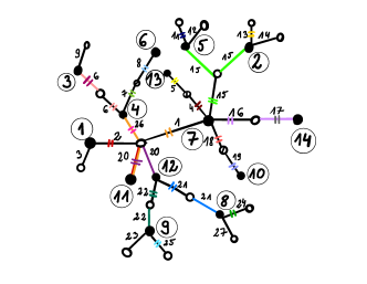
(a)

(b)

Figure 18. LABEL:sub@subfig:ex9 The outcome of applying two consecutive operations: $\mathbb{B}_{4,3}$ and $\mathbb{J}_{4,6}$ to the tree from Figure 14b.
LABEL:sub@subfig:ex10 The outcome of applying two consecutive operations: $\mathbb{B}_{7,2}$ and $\mathbb{B}_{7,5}$ to the tree from LABEL:sub@subfig:ex9.

(a)

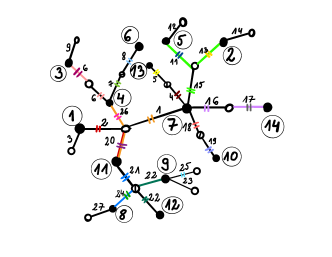
(b)

Figure 19. LABEL:sub@subfig:ex11 The output of $\mathbb{J}_{11,12}$ applied to the tree from Figure 18b. LABEL:sub@subfig:ex12 The output of $\mathbb{B}_{12,8}$ applied to the tree from LABEL:sub@subfig:ex11.

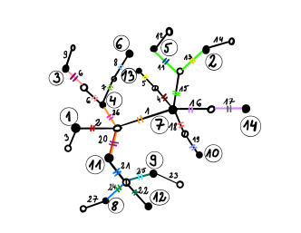
(a)

(b)

Figure 20. LABEL:sub@subfig:ex13 The output of $\mathbb{B}_{12,9}$ applied to the tree from Figure 18b.
LABEL:sub@subfig:ex14 The output of our algorithm $\mathcal{A}$ applied to the minimal factorization (13). It was created directly from the tree depicted on LABEL:sub@subfig:ex1.

For $C=6$ we have $\alpha_{6}=4$. Since $B_{6}\setminus\{4\}=\{3,6\}$ the loop runs over: $\bullet$  $y=3$ and we apply $\mathbb{B}_{4,3}$; see Figure 18a; $\bullet$ $y=6$ and we apply $\mathbb{J}_{4,6}$; see Figure 18a.

For $C=15$ we have $\alpha_{15}=7$. Since $B_{15}\setminus\{7\}=\{2,5\}$ the loop runs over: $\bullet$ $y=2$ and we apply $\mathbb{B}_{7,2}$; see Figure 18b; $\bullet$ $y=5$ and we apply $\mathbb{B}_{7,5}$; see Figure 18b.

For $C=20$ we have $\alpha_{20}=11$. Since $B_{20}\setminus\{11\}=\{12\}$, the internal loop is applied once with $y=12$. As a result we apply $\mathbb{J}_{11,12}$; see Figure 18a.

For $C=21$ we have $\alpha_{21}=12$. Since $B_{21}\setminus\{12\}=\{8\}$, the internal loop is applied once with $y=8$. As a result we apply $\mathbb{B}_{12,8}$; see Figure 18b.

For $C=22$ we have $\alpha_{22}=12$. Since $B_{22}\setminus\{12\}=\{9\}$, the internal loop is applied once with $y=9$. As a result we apply $\mathbb{B}_{12,9}$; see Figure 19a.

Figure 19b gives the output $T_{2}$ of our algorithm $\mathcal{A}$ applied to the minimal factorization (13). The result is a Stanley tree of type $(1^{14})$.

The resulting tree $T_{2}$ is the final output of our algorithm $\mathcal{A}$. In Section 3 we will show that it has the desired properties from 2.1.

2.8. Correctness of the rib treatment algorithm

The main result of this section is 2.7, which states that the rib treatment presented in Section 2.7 is well-defined in the sense that the assumptions for the bend and jump operations (Sections 2.3.1 and 2.4.1) are indeed fulfilled during the rib treatment.

For a black non-spine vertex $z$ by the branch defined by $z$ we mean the edge outgoing from $z$ in the direction of the spine together with all edges and vertices that are its descendants. The branch defined by $z$ will also be called the branch $z$.

Lemma 2.6.

For each black non-spine vertex $z$ the branch $z$ does not change during the action of the algorithm $\mathcal{A}$ until the vertex $z$ becomes touched.

Proof.

As the first step we notice that the algorithm $\mathcal{A}$ (i.e., the combined the spine part and the rib part) can be regarded as a sequence of jump and bend operations. We will use the induction over the number of bend/jump operations that have been performed so far.

At the beginning of the algorithm there is nothing to prove.

Let us take an arbitrary tree transformation $\mathbb{T}$ (with $\mathbb{T}=\mathbb{B}_{x,y}$ or $\mathbb{T}=\mathbb{J}_{x,y}$ for some black vertices $x,y$) in our algorithm; we denote by $T$ the value of the tree before the transformation $\mathbb{T}$ was applied. Our inductive hypothesis is that (i) the branch $z$ was unchanged before $\mathbb{T}$ was applied, and (ii) the vertex $z$ was untouched before $\mathbb{T}$ was applied. Let $E_{1}$ be the cluster defined in (B1) in Section 2.3.1, respectively in (J1) in Section 2.4.1, i.e., the cluster that contains the vertices $x$ and $y$.

In the case when $z=y$ then after performing the transformation $\mathbb{T}$ the vertex $z$ becomes touched and there is nothing to prove.

We will show that $x$ is touched. In the case when the black vertex $x$ in the original tree $T_{1}$ was a spine vertex there is nothing to prove. Consider now the case when $x$ in $T_{1}$ was a non-spine vertex; in this case the operation $\mathbb{T}$ is a part of the rib treatment algorithm. Let $c$ be the white vertex in the original tree $T_{1}$ that is the parent of the vertex $x$; it follows that in some moment before the operation $\mathbb{T}$ was applied, the variable in the external loop (either in the spine treatment algorithm or in the rib treatment algorithm) took the value $C=c$ and one of the operations: $\mathbb{J}_{\alpha_{c},x}$ or $\mathbb{B}_{\alpha_{c},x}$ was applied; since this moment the vertex $x$ was touched, as claimed. Since $z$ is assumed to be not touched, it follows that $z\neq x$.

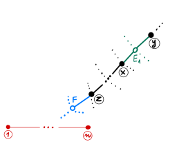
Figure 21. The hypothetical relative position of the cluster $E_{1}$ (green), the vertex $z$, the cluster $F$ (blue), and the spine (red) in the tree $T$ as long as the branch $z$ remains unchanged. We will prove that this configuration is not possible.

The above discussion shows that we may assume that $z\notin\{x,y\}$. We denote by $F$ the cluster in the tree $T_{1}$ that is defined by the edge outgoing from the vertex $z$ in the direction of the spine; we recall that $E_{1}$ is the cluster that contains the vertices $x$ and $y$. We will show that the cluster $E_{1}$ is not contained in the branch $z$, i.e., the situation depicted on Figure 21 is not possible. By contradiction, suppose that the cluster $E_{1}$ is contained in the branch $z$. By the inductive assumption, before $\mathbb{T}$ was applied, the branch $z$ remained unchanged, so the relative position of the spine, the vertex $z$ and the clusters $E_{1}$ and $F$ is the same in the initial tree $T_{1}$ and in the tree $T$; see Figure 21. It follows that $E_{1}$ is a non-spine cluster. Furthermore either $F$ is a spine cluster, or $F$ is a non-spine cluster that is a predecessor of $E_{1}$ in the sequence $\Sigma$. In particular, the transformation $\mathbb{T}$ was performed during the rib treatment part of the algorithm and the value of the variable $C$ in the main loop at this moment was equal to $C=E_{1}$. In one of the previous iterations of the main loop (either in the spine treatment or in the rib treatment) the variable $C$ took the value $C=F$; during this iteration of the loop the vertex $z$ became touched, which contradicts the inductive hypothesis.

The above observation that $E_{1}$ is not contained in the branch $z$ allows us to define the branch $z$ in an equivalent way by orienting all edges of the tree towards the cluster $E_{1}$ and saying that the branch $z$ consists of the edge outgoing from $z$ in the direction of $E_{1}$ with all edges and vertices that are its descendants. We will use this alternative definition in the following.

In the case when $\mathbb{T}=\mathbb{B}_{x,y}$ (see Figure 8a, where $z$ is any black vertex different than $x$ and $y$; note that this black vertex may be also in the part of the tree that was not shown), we can notice that the branch $z$ still does not change after the application of $\mathbb{T}$; see Figure 8b, as required.

Consider the case when $\mathbb{T}=\mathbb{J}_{x,y}$ and (with the notations from Section 2.4.1) $j=x$. See Figure 9a, where $z$ is any black vertex different than $x$ and $y$. We can notice that the branch $z$ still does not change after the application of $\mathbb{T}$, as required; see Figure 9b.

Consider now the remaining case when $\mathbb{T}=\mathbb{J}_{x,y}$ and $j\neq x$ (see Figure 10). If $z\neq j$ then the branch $z$ still does not change after the application of $\mathbb{T}$, as required. The case $z=j$ is is not possible because 2.2 (I4) applied to the cluster $E_{1}$ implies that $z$ is touched which contradicts the inductive assumption.

This completes the proof of the inductive step. ∎

Proposition 2.7.

For each operation bend (respectively, jump) performed during the rib treatment algorithm the assumptions (B1)–(B3) (respectively, the assumptions (J1)–(J4)) are fulfilled; in this way each bend/jump operation is well-defined.

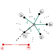
(a)

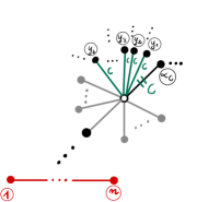
(b)

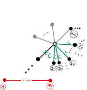
(c)

Figure 22. Three possible structures of the non-spine cluster $C$ at the beginning of the iteration of the external loop in the rib treatment algorithm.
LABEL:sub@subfig:rib1 This structure coincides with the original structure of $C$ in the input tree $T_{1}$. The edge outgoing from the center of the cluster $C$ in the direction of the spine is the root of the cluster $C$ and its black endpoint is the anchor $\alpha_{C}$ of the cluster.
LABEL:sub@subfig:rib2 This structure occurs as an outcome of either: (i) the bend operation in the parent cluster, provided that $C$ is the leftmost child, i.e., $C$ corresponds to the blue cluster $E_{2}$ with the notations of Figure 8, or (ii) the jump operation in the parent cluster, provided that $C$ is the second leftmost child, i.e., $C$ corresponds to the red cluster $E_{3}$ with the notations from Figures 10 and 10. This structure was obtained from LABEL:sub@subfig:rib1 by adding some additional vertices that do not belong to the cluster $C$; going clockwise these additional vertices occur after $\alpha_{C}$. The edge outgoing from the center of the cluster $C$ in the direction of the spine does not belong to the cluster $C$.
LABEL:sub@subfig:rib3 This structure occurs as an outcome of the jump operation in the parent cluster, provided that $C$ is the leftmost child, i.e., $C$ corresponds to $E_{1}$ with the notations from Figures 10 and 10. The root edge does not correspond to any of the edges that formed $C$ in the original tree $T_{1}$; in particular the black endpoint of the root does not belong to the set $B_{C}=\{\alpha_{C},y_{1},\dots,y_{l}\}$. The root of the cluster $C$ is in the direction of the spine. More specifically, the counterclockwise cyclic order of the edges with their black endpoints around the center of cluster $C$ is as follows: the root of the cluster $C$, the edges that belong to cluster $C$ with consecutive black endpoints $y_{1},\dots,y_{l}$, the edge that does not belong to the cluster $C$ with the black endpoint equal to the anchor $\alpha_{C}$ and the remaining edges that do not belong to the cluster $C$.

Proof.

We will go through some iteration of the external loop of the rib treatment for some specific value of the variable $C$ (i.e., $C$ is a non-spine cluster) and we will verify that all operations performed in this iteration are well-defined.

Consider the case when the anchor $\alpha_{C}$ is a non-spine vertex. By $C_{1}$ we denote the cluster that is the parent of the cluster $C$ in the tree $T_{1}$. Therefore, the black vertex $\alpha_{C}$ also belongs to the cluster $C_{1}$. During some previous iteration of the main loop either during the spine treatment or during the rib treatment (more specifically, this was the iteration when the variable $C$ took the value $C_{1}$) we performed an operation $\mathbb{T}$ with $\mathbb{T}=\mathbb{B}_{\alpha_{C_{1}},\alpha_{C}}$ or $\mathbb{T}=\mathbb{J}_{\alpha_{C_{1}},\alpha_{C}}$. From the above Lemma 2.6 it follows that until the operation $\mathbb{T}$ was performed, the branch defined by the black vertex $\alpha_{C}$ was unchanged, hence the cluster $C$ had the form depicted on Figure 22a.

In the case when $\mathbb{T}=\mathbb{B}_{\alpha_{C_{1}},\alpha_{C}}$ is a bend operation, after this operation $\mathbb{T}$ is applied the cluster $C$ either has the form depicted on Figure 22b (this happens if $C$ is leftist) or it still has the form depicted on Figure 22a (otherwise).

In the case when $\mathbb{T}=\mathbb{J}_{\alpha_{C_{1}},\alpha_{C}}$ is a jump operation, after this operation $\mathbb{T}$ is applied the cluster $C$ either has the form depicted on Figure 22c (this happens if $C$ is leftist), or the form depicted on Figure 22b (this happens if $C$ is the second leftmost child) or it still has the form depicted on Figure 22a (otherwise).

For each of the aforementioned three cases depicted on Figure 22 one can go through the internal loop (in a manner similar to that from the proof of the inductive step on the pages 2.6–2.6, but simpler) and to verify that the assumptions required by the bend/jump operations are indeed fulfilled, as required.

Now, we assume that $\alpha_{C}$ is a spine vertex. In this case we have two possible situations. The black vertex $\alpha_{C}$ belongs to either one or two spine clusters in the tree $T_{1}$.

Consider the case when the anchor $\alpha_{C}$ belongs to two spine clusters in the tree $T_{1}$, denoted by $C_{1},C_{2}$. During some previous iteration of the main loop of the spine treatment part (more specifically, this was the iteration when the variable $C$ took the value $C_{i}$ for $i=1,2$) we performed an operation $\mathbb{T}$ with

1. $\mathbb{T}=\mathbb{B}_{\alpha_{C_{i}},\alpha_{C}}$ if $\alpha_{C_{i}}<\alpha_{C}$,

2. $\mathbb{T}=\mathbb{B}_{\alpha_{C_{i}},\cdot}$ or $\mathbb{T}=\mathbb{J}_{\alpha_{C_{i}},\cdot}$ if $\alpha_{C_{i}}=\alpha_{C}$.

In the case (i), after this operation $\mathbb{T}=\mathbb{B}_{\alpha_{C_{i}},\alpha_{C}}$ is applied, the cluster $C$ either has the form depicted on Figure 22b (this happens if $C$ is leftist) or it still has the form depicted on Figure 22a (otherwise). By checking these two cases separately (the reasoning is fully analogous to the one presented above) we see that during this external loop iteration for this specific value of $C$ all the assumptions for the bend/jump operations are fulfilled, as required.

In the case (ii), after the operation $\mathbb{T}$ is applied the cluster $C$ still has the form depicted on Figure 22a. Again, one can easily check that that during this loop iteration all the assumptions for the bend/jump operations are fulfilled, as required.

In the case when the black vertex $\alpha_{C}$ belongs to only one spine cluster in the tree $T_{1}$ the reasoning is analogous to the one above and we skip the details. ∎

As an extra bonus, the above proof shows that any non-spine cluster $C$ at a later stage of the algorithm (as long as it remains untouched) either has the form LABEL:sub@subfig:rib1, LABEL:sub@subfig:rib2, or LABEL:sub@subfig:rib3 on Figure 22.

3. The output of the bijection is a Stanley tree

The following results are the first step towards the proof of 2.1.

Lemma 3.1.

Let $\mathbb{J}_{x,y}$ be one of the jump operations performed during the execution of the algorithm $\mathcal{A}$, and let $j$ be the corresponding black vertex that was defined in the assumption (J2) from Section 2.4.1; see Figures 10 and 10. Then the label of the vertex $j$ is smaller than the label of the vertex $y$.

Proof.

Our strategy is to explicitly pinpoint the vertex $j=j(x,y)$ in the original tree $T_{1}$.

We start with the case when the jump operation $\mathbb{J}_{x,y}$ was performed during the spine treatment (this case holds true if and only if the white vertex between $x$ and $y$ is a spine vertex). Let $C$ be the value of the external loop variable at the time when $\mathbb{J}_{x,y}$ was performed. We have shown in 2.5 that the anchor of the cluster $C$ is the endpoint of the root of the cluster $C$ in each step of the internal loop. Therefore $j=x$; see the case described on Figure 10.

Consider now the case when the jump operation $\mathbb{J}_{x,y}$ was performed during the rib treatment; again let $C$ be the value of the external loop variable at the time when $\mathbb{J}_{x,y}$ was performed; in particular $C$ is a non-spine cluster.

If the cluster $C$ in the tree $T_{1}$ is non-leftist, from Lemmas 2.3 and 2.4 we infer that no bend/jump operation separated the anchor of the cluster $C$ with the root of this cluster. It follows therefore that $j=x$; see the case described on Figure 10.

Consider now the case when the cluster $C$ in the tree $T_{1}$ is leftist. From Lemmas 2.3 and 2.4 it follows that in order to check whether the anchor of the cluster $C$ is separated from the root, we need to consider one of the previous iterations of the main loop (in the spine treatment or the rib treatment), namely the one for the cluster $C^{\prime}$ that is the parent of $C$. In the case when $x<\alpha_{C^{\prime}}$, this previous iteration contained the bend operation $\mathbb{B}_{\alpha_{C^{\prime}},x}$, which does not separate the anchor from the root, so again $j=x$.

The only challenging case is the one when $C$ is a leftist cluster and $x>\alpha_{C^{\prime}}$ so that this previous iteration contains the jump operation $\mathbb{J}_{\alpha_{C^{\prime}},x}$, which separated the anchor and the root in the cluster $C$. Let us have a closer look on this previous jump operation $\mathbb{J}_{\alpha_{C^{\prime}},x}$; it is depicted on Figures 10 and 10 with the blue cluster $E_{2}=C$ and the black cluster $E_{1}=C^{\prime}$. Our desired value of $j(x,y)$ is the black endpoint of the root of the cluster $C$; on Figures 9b and 9b this endpoint carries the label $j$. On the other hand, the value of the variable $j=j(\alpha_{C^{\prime}},x)$ for the previous jump operation $\mathbb{J}_{\alpha_{C^{\prime}},x}$ in the parent cluster is the black endpoint of the root of the cluster $C^{\prime}=E_{1}$; on Figures 9a and 9a this vertex carries the same label $j$. In this way we proved that our desired value of

$$j=j(x,y)=j(\alpha_{C^{\prime}},x)$$

coincides with the value of $j$ for the jump operation $\mathbb{J}_{\alpha_{C^{\prime}},x}$ in the parent cluster. It follows that the value of $j$ can be found by the following recursive algorithm.

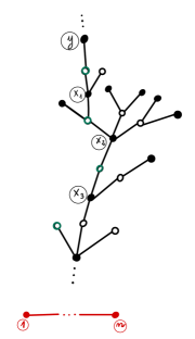
Figure 23. The tree $T_{1}$ with black vertices $y,x_{1},x_{2},x_{3}$ where a white leftist vertices are marked green.

We traverse the tree $T_{1}$, starting from the black vertex $y$, always going towards the spine, as long as the following two conditions are satisfied:

1. we are allowed to enter a white vertex only if it is a leftist vertex;

2. we are allowed to enter a black vertex only if its label is smaller than the label of the last visited black vertex so far.

Additionally, if we just entered a black spine vertex, the algorithm terminates. If we entered a white spine vertex $w$ it is not clear what it means to move towards the spine; we declare that we should move now to the the root $\alpha_{w}$ of the cluster defined by $w$. We denote by $z=(z_{1},\dots,z_{l})$ the labels of the visited black vertices. For the example on Figure 23 if $x_{3}<x_{2}<x_{1}<y$ we have $z=(y,x_{1},x_{2},x_{3})$. The label $z_{l}$ of the last visited black vertex is the label of our searched black vertex $j$. It is obvious now that $j<y$. ∎

Proposition 3.2.

The output of the algorithm $\mathcal{A}$ from Section 2 belongs to $\mathcal{T}_{b_{1},\dots,b_{n}}$.

Proof.

Recall that the integers $a_{1},\dots,a_{n}$ are related to $b_{1},\dots,b_{n}$ via (12).

By construction, the initial tree $T_{1}$ has $n$ black vertices labeled with the numbers $1,\dots,n$, and $k$ white vertices, and $\sum_{i}a_{i}=n+k-1$ edges labeled with the numbers $1,\dots,k$ in such a way that each edge label is used at least once, cf. (9). By counting the number of edges we observe that

$$\sum_{c=1}^{k}|B_{c}|=n+k-1.$$

Furthermore, if $c\in\{1,\dots,k\}\setminus(\mathfrak{C}\cup\Sigma)$, so that the corresponding cluster is a leaf, then $|B_{c}|=1$. It follows that the total number of jump/bend operations during the execution of our algorithm $\mathcal{A}$ is equal to

(15) $$\sum_{c\in\mathfrak{C}}(|B_{c}|-1)+\sum_{c\in\Sigma}(|B_{c}|-1)=\\ =\sum_{c\in\mathfrak{C}}(|B_{c}|-1)+\sum_{c\in\Sigma}(|B_{c}|-1)+\sum_{c\in\{1,\dots,k\}\setminus\{\mathfrak{C}\cup\Sigma\}}(|B_{c}|-1)=\\ =\left(\sum_{c=1}^{k}|B_{c}|\right)-k=n-1.$$

After performing each bend/jump operation, the number of white vertices as well as the number of edges decreases by $1$. Furthermore, the edge that disappears has a repeated label, in this way the set of the edge labels remains unchanged in each step.

It follows that the output $T_{2}$ is a bicolored plane tree with $(n+k-1)-(n-1)=k$ edges labeled by numbers $1,\dots,k$ (so each label is used exactly once) and with $k-(n-1)=\sum_{i=1}^{n}b_{i}$ white vertices, cf. (4). To complete the proof we have to show that the tree $T_{2}$ is a Stanley tree of type $(b_{1},\dots,b_{n})$.

We will consider two types of edges: solid and dashed. At the beginning in the plane tree $T_{1}$ each edge is declared to be solid. After performing the operation $\mathbb{B}_{x,y}$ the two edges that form the path between $x$ and $y$ become dashed; see Figure 8b. After performing the operation $\mathbb{J}_{x,y}$ the two edges that form the path between $j$ and $y$ become dashed; see Figures 9b and 9b.

We say that a white white vertex $v$ is attracted to a black vertex $i$ if one of the following two conditions holds true:

• the vertices $i$ and $v$ are connected by a solid edge,

• the vertices $i$ and $v$ are connected by a dashed edge and

  $$\max\big{\{}y\mathrel{\mathop{\ordinarycolon}}\emph{$y$ and $v$ are connected by a dashed edge}\big{\}}=i.$$

If $v$ is attracted to $i$, we will also say that the edge $e$ between $v$ and $i$ is attracted to $i$ or that $e$ is an attraction edge.

For each $i\in\{1,\dots,n\}$ we define the variable $\mathfrak{b}_{i}$; in each step of the algorithm this variable counts the number of white white vertices that are attracted to the black vertex $i$.

By considering any bend/jump operation that is performed during the algorithm $\mathcal{A}$ it is easy to see that each of the variables $\mathfrak{b}_{1},\dots,\mathfrak{b}_{n}$ weakly decreases over time. The only difficulty in the proof is to verify that during the jump operation the newly created vertex $w$ (with the notations from Figures 10 and 10) is not attracted to the vertex $j$; this fact is a consequence of 3.1. Below we will show that for $i\in\{2,\dots,n-1\}$ the variable $\mathfrak{b}_{i}$ during the algorithm $\mathcal{A}$ decreases at least by $2$, while each of the variables $\mathfrak{b}_{1}$ and $\mathfrak{b}_{n}$ decreases at least by $1$.

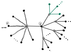
(a)

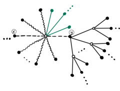
(b)

Figure 24. LABEL:sub@subfig:exA1 The initial configuration of the tree. Wavy edge means that this edge can be solid or dashed.
LABEL:sub@subfig:exA2 The structure of the tree LABEL:sub@subfig:exA1 after performing the operation $\mathbb{B}_{x,y}$ with $x>y$.

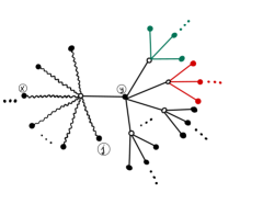
(a)

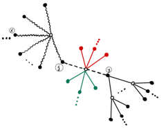
(b)

Figure 25. LABEL:sub@subfig:jumpA1 The initial configuration of the tree. Wavy edge means that this edge can be solid or dashed. We recall that $j<y$ by 3.1.
LABEL:sub@subfig:jumpA2 The structure of the tree LABEL:sub@subfig:jumpA1 after performing the operation $\mathbb{J}_{x,y}$ with $x<y$.

Case 1: $i$ is a non-spine vertex. For convenience we will denote the non-spine black vertex $i$ by the symbol $y$. There exists exactly one cluster $c\in\{1,\dots,k\}$ in the direction of the spine in the plane tree $T_{1}$ such that $y\in B_{c}$. In the iteration of the main loop (in the spine treatment or in the rib treatment) corresponding to $C=c$ one of the following operations is applied: either $\mathbb{B}_{\alpha_{c},y}$ (if $y<\alpha_{c}$; see Figure 25) or $\mathbb{J}_{\alpha_{c},y}$ (otherwise; see Figure 25). By Lemma 2.6 it follows that at the time one of these operations is applied, the edges in the branch $y$ are solid; on Figures 24a and 24a this branch is located on the right-hand side and drawn with non-wavy lines. By looking on Figures 25 and 25 we see that for either of these two operations $\mathfrak{b}_{y}^{\text{after}}=\mathfrak{b}_{y}^{\text{before}}-2$, as required.

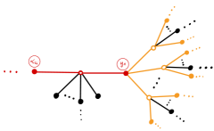
(a)

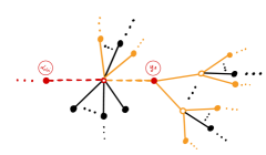
(b)

Figure 26. LABEL:sub@subfig:proofspineA The initial configuration of the tree $T_{1}$. The black vertices $\alpha_{c_{i}},y_{1}$ are spine and such that $\alpha_{c_{i}}<y_{1}$. The orange edges mark one of the possible pathways of the spine.
LABEL:sub@subfig:proofspineB The structure of the tree LABEL:sub@subfig:proofspineA after performing the operation $\mathbb{B}_{\alpha_{c_{i}},y_{1}}$.

Case 2: $i$ is a spine vertex. Note that in the spine treatment any two bend operations commute. Furthermore, any jump operation performed in a given spine cluster does not affect the remaining spine clusters. Therefore, the final output does not depend on the order in which we choose the clusters from $\mathfrak{C}$. For this reason we may start the analysis of the time evolution of any spine cluster $C$ from the input tree $T_{1}$ where all edges are solid (i.e., we may assume that the external loop is executed first for the cluster $C$).

If $i\in\mathcal{B}\setminus\{1,n\}$ is not one of the endpoints of the spine, it belongs to exactly two spine clusters $c_{1},c_{2}$ in the plane tree $T_{1}$. Let us fix some $j\in\{1,2\}$; with the notations of Figure 11a, $i\in\{\alpha_{c_{j}},y_{1}\}$ is one of the two spine vertices in the cluster $c_{j}$ and $\mathbb{B}_{\alpha_{c_{j}},y_{1}}$ is one of the operations that are performed in the iteration of the external loop in the spine treatment for $C=c_{j}$. From Figure 26 it follows that for each spine vertex $v\in\{\alpha_{c_{j}},y_{1}\}$ in this cluster $\mathfrak{b}_{v}^{\text{after}}=\mathfrak{b}_{v}^{\text{before}}-1$. Since there are two choices for $j\in\{1,2\}$ it follows that the variable $\mathfrak{b}_{i}$ decreases (at least) twice during the whole algorithm, as required.

An analogous argument shows that if $i\in\{1,n\}$ is one of the endpoints of the spine then the variable $\mathfrak{b}_{i}$ decreases (at least) once during the whole algorithm, as required.

At the beginning of the algorithm $\mathfrak{b}_{i}^{\text{initial}}=a_{i}$ for each $i\in\{1,\dots,n\}$. The above discussion shows therefore that in the output tree $T_{2}$

(16) $$\mathfrak{b}^{\text{final}}_{1}\leq a_{1}-1,\quad\mathfrak{b}^{\text{final}}_{2}\leq a_{2}-2,\quad\dots,\quad\mathfrak{b}^{\text{final}}_{n-1}\leq a_{n-1}-2,\quad\mathfrak{b}^{\text{final}}_{n}\leq a_{n}-1.$$

It follows that

$$\sum_{i=1}^{n}\mathfrak{b}^{\text{final}}_{i}\leq\sum_{i=1}^{n}(a_{i}-1)-(n-2)=(k-1)-(n-2)=k-(n-1),$$

where we used the relationship (9). In each step of the algorithm each white vertex is attracted to at least one black neighbor; it follows that the left-hand side of the above inequality is an upper bound for the number of white vertices in the output tree $T_{2}$.

On the other hand, from the first part of the proof we know that the output tree $T_{2}$ has exactly $k-(n-1)$ white vertices and the above inequality is saturated:

(17) $$\sum_{i=1}^{n}\mathfrak{b}^{\text{final}}_{i}=k-(n-1).$$

It follows that each white vertex is attracted to exactly one black neighbor; also the tree $T_{2}$ is a Stanley tree of type $(\mathfrak{b}^{\text{final}}_{1},\dots,\mathfrak{b}^{\text{final}}_{n})$. If at least one of the inequalities (16) was strict, this would contradict (17). We proved in this way that $\mathfrak{b}^{\text{final}}_{i}=b_{i}$, which is given by (12), which completes the proof. ∎

Remark 3.3.

The algorithm has one random component in it, namely when we choose the ordering for $\Sigma$ on Page 6. In fact, this choice of the ordering does not impact the outcome of the algorithm. Probably the best way to prove it is to use the alternative description of the algorithm which we provide in Section 4 which is fully deterministic and does not refer to such choices.

4. Alternative description of the bijection

In the current section we will provide an alternative description of the bijection $\mathcal{A}$. This alternative viewpoint on $\mathcal{A}$ will be essential for the construction of the inverse map $\mathcal{A}^{-1}$ in Section 5.

Recall that the spine in the output tree $T_{2}$ is the path connecting the two black vertices with the labels $1$ and $n$. We orient the non-spine edges of the tree $T_{2}$ in the direction of the spine. In this way we can view the plane tree $T_{2}$ as a path (=the spine) to which there are attached plane trees. With this perspective in mind, the output tree $T_{2}$ will turn out to be uniquely determined by: the local information about the structure of white non-spine vertices, the local information about the structure of black non-spine vertices, and the information about the spine and its small neighborhood. The aforementioned local information for a black non-spine vertex $y$ is just the list of the labels of the edges connecting $y$ to its children. For a white non-spine vertex the local information contains more data; see Section 4.2. This local information will be provided separately for white non-spine vertices (Sections 4.1 to 4.4) and for certain black non-spine vertices (Section 4.6). Finally, in Sections 4.9 and 4.10 we will describe the spine vertices of $T_{2}$ as well as its neighborhood.

4.1. White vertices: organic versus artificial

Recall that in the description of the jump operation in Section 2.4.2 the newly created white vertex $w$ (see Figures 9b and 9b) was declared to be artificial. Each white vertex that was not created in this way by some jump operation will be referred to as organic. More precisely, we declare that all white vertices in the initial tree $T_{1}$ are organic. The bend operation can be viewed as merging two white vertices (with the notations of Figure 8a these are the vertices $v_{1}$ and $v_{2}$); it turns out that for each bend operation that is performed during the execution of the algorithm the vertex $v_{2}$ is organic. We declare that the vertex created by merging $v_{1}$ and $v_{2}$ is organic (respectively, artificial) if and only if $v_{1}$ was organic (respectively, artificial).

4.2. Direct neighborhood of a white non-spine vertex

For any non-spine white vertex $w$ of $T_{2}$ we will describe the direct neighborhood of $w$ that is defined as:

• the labels of the children of $w$, together with the labels of the corresponding edges, and

• the label of the parental edge of $w$, defined as the edge that connects $w$ with its parent (however, we are not interested in the label of this parent).

We will describe such direct neighborhoods separately for white non-spine organic vertices and for white non-spine artificial vertices.

4.3. Direct neighborhood of white non-spine organic vertices in the output tree $T_{2}$

Our starting point is the tree $T_{1}$. Our goal in this section is to find all non-spine organic white vertices in $T_{2}$ and then for each such a vertex to describe its direct neighborhood. For this reason we disregard now all artificial white vertices as well as the information about the children of the black vertices.

4.3.1. The first pruning

With this quite narrow perspective in mind, each jump operation (with the notations from Figures 10 and 10) can be seen as removal of the edge $E_{1}$ between $y$ and $v_{1}$ as well as removal of the white vertices $v_{2}$ and $v_{3}$. The remaining children of $y$ (i.e., the white vertices $v_{4},v_{5},\dots$) remain intact, but we are not interested in keeping track of the parents of white vertices (we are interested in keeping track of just the label of the parental edge for a white vertex). Still keeping our narrow perspective in mind, it follows that the application of all jump operations in the rib treatment part of the algorithm (Section 2.7) is equivalent to the following first pruning procedure:

for each non-spine white vertex $v_{1}$ and its child $y$ that carries a bigger label than its grandparent (i.e., $y>\alpha_{v_{1}}$) we remove:

• the vertex $y$ together with the edge that points towards its parent,

• the two leftmost children of $y$ (with the notations of Figures 10 and 10 they correspond to $v_{2}$ and $v_{3}$) together their children, and the edges that connect them.

The side effect of the removal of the vertex $y$ is that each of the edges $E_{4},E_{5},\dots$ (which formerly connected $y$ to its non-two-leftmost children) has only one endpoint, namely the white one.

Remark 4.1.

Later on we will use the following observation: our initial choice of the cyclic order of the edges around white vertices (Section 2.1.1) implies that after this pruning, for each white non-spine vertex $w$ the labels of its remaining children are arranged in an increasing way from right to left; furthermore, each of these labels is smaller than the label of the parent of $w$, i.e., $\alpha_{w}$.

4.3.2. The second pruning

If an edge between a non-spine white vertex $w$ and its child $b$ still remains after the above pruning procedure, this means that during the execution of the algorithm $\mathcal{A}$ a bend operation $\mathbb{B}_{\alpha_{w},b}$ was performed. With the notations of Figure 8a this operation does not affect the white vertices $v_{3},v_{4},\dots$ (i.e., the children of the vertex $y=b$ except for the leftmost child). With our narrow perspective in mind, we are not interested in keeping track of the parent of these vertices, which motivates the following second pruning procedure:

we disconnect each black non-spine vertex $b$ from the edges connecting $b$ with each of its children, with the exception of the leftmost child.

Again, as an outcome of this disconnection there are some edges that have only one endpoint, the white one.

Note that since in the initial tree $T_{0}$ the degree of each black vertex was at least $2$, in the outcome of the second pruning each black non-spine vertex has degree equal exactly to $2$. Our analysis of the impact of the bend operation $\mathbb{B}_{\alpha_{w},b}$ is not complete yet and will be continued in a moment.

4.3.3. Folding

After performing the above two pruning operations, the tree splits into a number of connected components. Let $T$ be one of these connected components that are disjoint with the spine; it is an oriented tree, which has a white vertex $v$ as the root. Additionally, this root $v$ has a special edge (the parental edge) that is pointing in the former direction of the spine; this edge has only one endpoint.

Consider some black vertex $b\in T$. Its degree is equal to $2$ and the aforementioned bend operation $\mathbb{B}_{\alpha_{w},b}$ can be seen as a counterclockwise rotation of the edge that connects $b$ with its only child towards the edge that connects $b$ with its parent so that these two edges are merged into a single edge (see Figure 27). The label of the merged edge is declared to be the label of the edge that formerly connected $b$ with its child, with the notations of Figure 27 this label is equal to $e$. As a result of the edge merging, a pair of white vertices – the child of $b$, and the parent of $b$ – is merged into a single white vertex and the vertex $b$ becomes a leaf. After the above folding procedure is applied iteratively to all black vertices in $T$, the connected component $T$ becomes a single white vertex connected to a number of black vertices, and together with the parental edge of the root. For an example see Figure 28.

(a)

(b)

Figure 27. LABEL:sub@subfig:bending2in The initial configuration of a part of the tree $T$. Additional labels on this figure will be explained and used in Section 5.3.5.
LABEL:sub@subfig:bending2out The outcome of folding at the vertex $b$.

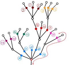
(a)

(b)

Figure 28. LABEL:sub@subfig:bendingin Example of a connected component $T$ that has a white root of the output of the two pruning procedures. For simplicity the edge labels are not shown. The black vertices having the same parent were drawn with the same color. The thin red line with the arrows indicates the beginning of the depth-first search traversing of the tree; the black vertices are visited in the order $14,2,11,18,8,4,\dots$ (only the first visit in a given vertex is listed).
LABEL:sub@subfig:bendingout The output of the folding procedure applied to the tree $T$ from LABEL:sub@subfig:bendingin.

The above folding procedure can be described alternatively as follows: we traverse the tree $T$ by the depth-first search, starting at the root and touching the edmges by the left hand. For example, the beginning of such a depth-first search is indicated on Figure 28a by the red line with an arrow. We order the black vertices according to the time of the first visit in a given vertex. This order coincides with the children of the root $v$ (listed in the counterclockwise order) in the output of folding applied to $T$.

4.3.4. Conclusion

To summarize the current subsection: there is a bijective correspondence between (i) the white non-spine organic vertices in the output tree $T_{2}$, and (ii) the connected non-spine components of the outcome of the two pruning procedures. The children of such white organic non-spine vertices in $T_{2}$ can be found by the above depth-first traversing of the connected component. This observation will critical for the construction of the inverse map $\mathcal{A}^{-1}$.

4.4. Direct neighborhood of white non-spine artificial vertices in the output tree $T_{2}$

Our goal in this section is to find all non-spine artificial white vertices in $T_{2}$ and then for each such a vertex to find its direct neighborhood.

Each white artificial vertex $w$ is created during the execution of some jump operation $\mathbb{J}_{x,y}$ so there is a bijective correspondence between the artificial white vertices and the collection of certain pairs $(x,y)$, where $x$ and $y$ are black vertices such that $x$ is a grandparent of $y$ and $x<y$, cf. Figures 10 and 10. Let us fix the values of $w$, $x$, and $y$; we shall describe now the children of $w$. For this reason we will disregard tracking of the children of the black vertices as well as we will disregard these white vertices that will not be merged with $w$ by some bend operations.

After creation, the vertex $w$ may gain children only by the application of some bend operations. It follows that we may restrict our attention only to the descendants of the vertex $w$ and disregard the remaining part of the tree. This observation motivates the following procedure.

We apply the jump operation $\mathbb{J}_{x,y}$ to the initial tree $T_{1}$. The resulting tree has a unique artificial white vertex, which is denoted by $w$, as above. Then we keep only the vertex $w$, the edge adjacent to $w$ that is in the direction of the spine, and the descendants of $w$. We remove the remaining part of the tree.

A discussion analogous to the one from Section 4.3 motivates the following first pruning procedure:

for each remaining white vertex $w^{\prime}$ and each child $b$ of $w^{\prime}$ that carries a bigger label than its grandparent (i.e., $b>\alpha_{w^{\prime}}$) we remove the vertex $b$ and all of its descendants,

as well as the following second pruning procedure:

for each remaining black vertex $b$ and each child $w^{\prime}$ of $b$ that is not left-most, we remove the edge between $b$ and $w^{\prime}$ as well as the vertex $w^{\prime}$, all of its descendants, and all edges between them.

The outcome is a tree, which has the white artificial vertex $w$ as the root. Furthermore, each black vertex has degree $2$. Exactly as in Section 4.3.3, we apply folding to this tree; as a result we obtain a tree, which consists of a single white vertex $w$ as the root, which is connected to some number of black vertices. Additionally, the root $w$ is connected to the parental edge, which has only one endpoint. This tree is equal to the direct neighborhood of the artificial white vertex $w$ in the output tree $T_{2}$.

Figure 29. The neighbors of an artificial white vertex $w$ in the output tree $T_{2}$; see Figures 9b and 9b. The vertex $j$ is the parent of $w$. The blue vertices $a,b,c$, and the other adjacent blue vertices are the outcome of the pruning and folding of the blue tree on Figures 9a and 9a that starts with the edge $E_{2}$. The red vertices $d,e,f$, and the other adjacent red vertices are the outcome of the pruning and folding of the red tree on Figures 9a and 9a that starts with the edge $E_{3}$. By Remark 4.1 and 3.1 the vertex $y$ carries the biggest label among all neighbors of $w$.

To summarize: the set of all neighbors of an artificial vertex $w$ together with the information about their cyclic order looks like on Figure 29. A consequence Remark 4.1 and 3.1 is that the vertex $y$ carries the biggest label among all neighbors of $w$ in the output tree $T_{2}$.

4.5. Children of black vertices: how to name the white vertices?

For a given black non-spine vertex we intend to find the list of its children in the output tree $T_{2}$. Each such child is a white non-spine vertex, and in Sections 4.3 and 4.4 we already found the collection of such vertices. Now we need some naming convention that would allow to match each child to some white vertex from Sections 4.3 and 4.4. In this way a person who has the access to the tree $T_{1}$ but has no access to the tree $T_{2}$ would still be able to distinguish the white non-spine vertices of $T_{2}$. Our naming convention will be defined separately for the white organic and for the white artificial vertices.

In Section 4.3 we showed that each white organic vertex $w$ in $T_{2}$ is an outcome of folding applied to a certain tree $T$; in order to name $w$ we will identify it with the root of the tree $T$ (which is just a white vertex in $T_{1}$).

To each white artificial vertex $w$ of the tree $T_{2}$ we associate the largest label of its neighbors; see Figure 29. This largest label $y$ is an element of the set $\{1,\dots,n\}$ and can be identified with a black vertex in the tree $T_{1}$. The discussion from Section 4.4 shows that this map is injective and allows us to pinpoint uniquely each artificial white vertex. Furthermore, the label $y$ has the following natural interpretation: the artificial vertex $w$ was created by some jump operation of the form $\mathbb{J}_{\cdot,y}$.

With these conventions we will give the children of a non-spine black vertex in $T_{2}$ in the form of a list of (black and white) vertices of the tree $T_{1}$.

4.6. Children of black never-spine vertices

Consider a black vertex $y$ that in the input tree $T_{1}$ was not a spine vertex. It turns out (we will prove it later in Sections 4.9 to 4.10) that the vertex $y$ in the output tree $T_{2}$ is still not a spine vertex; in the following we will describe the children of $y$ in $T_{2}$ as well as the labels on the edges connecting $y$ with its children.

Recall that we oriented all non-spine edges in the tree $T_{1}$ towards the spine. Now, we additionally orient some spine edges in $T_{1}$ in such a way that for each white spine vertex $w$ its parent is equal to the root $\alpha_{w}$ of the corresponding cluster. With this convention, we denote by $x$ the grandparent of $y$. It follows that during the action of the algorithm $\mathcal{A}$ exactly one of the following two operations was performed: either the bend operation $\mathbb{B}_{x,y}$ (in the case when $x>y$) or the jump operation $\mathbb{J}_{x,y}$ (in the case when $x<y$).

4.7. Children of a black never-spine vertex, the case when $x>y$

4.7.1. The tree $T$

In this case the bend operation $\mathbb{B}_{x,y}$ was performed. As a result, the edge connecting $y$ to its leftmost child in $T_{1}$ is not among the edges that connect $y$ to its children in $T_{2}$. The other (i.e., the non-leftmost) edges connecting $y$ to its children in $T_{1}$ will remain in $T_{2}$; these edges will connect $y$ to its organic children. On the other hand, the vertex $y$ may gain some new, artificial children as an outcome of some jump operations. We will discuss them in the following.

Recall that with the notations of Figures 10 and 10 we denote by $j=j(x^{\prime},y^{\prime})$ the black vertex that as a result of a jump operation $\mathbb{J}_{x^{\prime},y^{\prime}}$ gains a new child, which is a white artificial vertex. This vertex $j$ is given in terms of the input tree $T_{1}$ by the algorithm contained in the proof of 3.1. The problem that we currently encounter is roughly the opposite: for a given black vertex $y$ of $T_{1}$ we should find all its artificial children in the output tree $T_{2}$ or, equivalently, all jump operations $\mathbb{J}_{x^{\prime},y^{\prime}}$ performed during the algorithm for which $y=j(x^{\prime},y^{\prime})$. Our strategy is to construct a certain tree $T$ that is a subtree of $T_{1}$. This plane tree will have the vertex $y$ as the root, and it will have the following two properties:

• whenever $x^{\prime},y^{\prime}$ are black vertices in $T_{1}$ such that $\mathbb{J}_{x^{\prime},y^{\prime}}$ is one of the operations performed during the algorithm $\mathcal{A}$ then

  $$j(x^{\prime},y^{\prime})=y\quad\iff\quad x^{\prime},y^{\prime}\in T,$$

• if $x^{\prime},y^{\prime}$ are black vertices in $T$ such that $x^{\prime}$ is the grandparent of $y^{\prime}$ then $\mathbb{J}_{x^{\prime},y^{\prime}}$ is one of the operations performed during the algorithm $\mathcal{A}$ (or, equivalently, $x^{\prime}<y^{\prime}$).

In this way there will be a bijection between the black non-root vertices of the tree $T$ and the artificial children of the vertex $y$ in $T_{2}$, which maps the black vertex $y^{\prime}$ to the artificial white vertex created during the operation of the form $\mathbb{J}_{\cdot,y^{\prime}}$.

4.7.2. The prunings

As the first step towards the construction of the tree $T$ we perform the following zeroth pruning:

in the tree $T_{1}$ we keep only the vertex $y$ and its offspring.

Recall that the bend operation $\mathbb{B}_{x,y}$ was performed and the edge connecting $y$ to its leftmost child in $T_{1}$ is not among the edges that connect $y$ to its children in $T_{2}$. This motivates the following operation.

Additionally, we remove the label from the edge connecting $y$ to its leftmost child.

The condition (C2) from the algorithm contained in the proof of 3.1 motivates the following first pruning procedure:

for each remaining white vertex $v_{1}$ and its child $y^{\prime}$ that carries a smaller label than its grandparent we remove the edge connecting $v_{1}$ with $y^{\prime}$, as well as the vertex $y^{\prime}$ and its offspring, as well as the edges connecting them.

Compare this to Section 4.3.1 where we removed each vertex that is bigger than its grandparent. As a result, the following analogue of Remark 4.1 holds true.

Remark 4.2.

Later on we will use the following observation: our initial choice of the cyclic order of the edges around white vertices (Section 2.1.1) implies that after this pruning, for each white non-spine vertex $w$ the labels of its remaining children are arranged in a decreasing way in the clockwise order; furthermore, each of these labels is bigger than the label of the parent of $w$, i.e., $\alpha_{w}$.

The other condition (C1) from the algorithm contained in the proof of 3.1 motivates the following second pruning procedure:

for each remaining black vertex $y^{\prime}$ such that $y^{\prime}\neq y$ is not the root vertex we remove all non-leftist children of $y^{\prime}$ as well as their offspring and all adjacent edges.

We denote by $T$ the outcome of these prunings. This tree has the property that the degree of each black vertex (with the exception of the root) is equal to $2$.

4.7.3. Jump operation as a replacement

Let $w$ be a child of the root vertex $y$. We start with the case when $w$ is not the leftmost child of $y$. Let the black vertices $V_{1},\dots,V_{d}$ be the children of $w$, listed in the clockwise order. After applying the jump operations that correspond to the cluster $w$ the whole subtree of $T$ that has $w$ as the root is replaced by the following collection of trees attached to the root (we list these trees in the clockwise order):

(18) $$(\text{the single organic vertex $w$}),\\ (\text{an artificial white vertex that carries the name $V_{1}$}\\ \text{to which there is an attached tree $T_{V_{1}}$ that was formerly attached to $V_{1}$}),\\ \dots,\\ (\text{an artificial white vertex that carries the name $V_{d}$}\\ {\text{to which there is an attached tree $T_{V_{d}}$ that was formerly attached to $V_{d}$});}$$

above we used the naming convention for white vertices from Section 4.5.

In the case when $w$ is the left-most child, the above discussion remains valid, however one should remove the first entry of the list (18), i.e., the single organic vertex $w$.

Each tree $T_{V_{i}}$ has a white vertex as the root, let the black vertices $W_{1},\dots,W_{e}$ be is children. Now, performing all jump operations in the cluster defined by this root corresponds to replacing the following item from the aforementioned list:

$$(\text{the artificial white vertex that carries the name $V_{i}$}\\ {\text{to which there is attached tree the $T_{V_{i}}$})}$$

by the following collection of trees attached to the root $y$:

$$(\text{the artificial white vertex that carries the name $V_{i}$}),\\ (\text{an artificial white vertex that carries the name $W_{1}$}\\ \text{to which there is an attached tree that was formerly attached to $W_{1}$}),\\ \dots,\\ (\text{an artificial white vertex that carries the name $W_{e}$}\\ {\text{to which there is an attached tree that was formerly attached to $W_{e}$}).}$$

We iteratively apply these replacements until each child of the root $y$ is a leaf. When the algorithm terminates, the ordered list of the children of the root $y$ in the output coincides with the ordered list of the children of the vertex $y$ in the tree $T_{2}$ that we are looking for. With the convention from Section 4.5, the children of $y$ (listed in the clockwise order) can be identified with a list of (black and white) vertices of the input tree $T_{1}$. In the following we will provide a more direct way of finding this list based only on the tree $T$. In fact, the elements of the list that we construct will provide more information; each entry of the list will be a pair of the form

(19) $$\big{(}(\text{name of a white vertex $w$}),\quad(\text{the label of the edge connecting $v$ and $w$})\big{)}.$$

4.7.4. The depth-first search

The recursive algorithm from Section 4.7.3 is just a complicated way of performing the depth-first search on the tree $T$. We traverse the tree $T$ by keeping it with the right hand (note that in the analogous depth-first search in Section 4.3.3 we touched the tree with the left hand). When we enter a non-root vertex $v$ for the first time, we proceed as follows:

• if $v$ is a white vertex that is a child of the root $y$ but not the left-most child of the root (each such a vertex corresponds to an white organic child of $y$ in $T_{2}$), we append the list with the pair

  $$\big{(}v,\quad(\text{the label of the edge connecting $v$ and $y$})\big{)},$$

  [note that during the zeroth pruning we removed the label from the leftmost edge of the root so that it is not listed here];

• if $v$ is a black vertex (each such a vertex corresponds to a white artificial child of $y$ in $T_{2}$) we append the list with the pair

  $$\big{(}v,\quad(\text{the label of the edge connecting $v$ with its unique child in $T$})\big{)}.$$

This procedure can be regarded as an analogue of folding from Section 4.3.3. This completes the description of the local information about the children of a black never-spine vertex $y$ in the case when $x>y$.

4.8. Children of a black never-spine vertex, the case when $x<y$

We plan to proceed in an analogous way as in Section 4.7. In this case the jump operation $\mathbb{J}_{x,y}$ was performed. We with the conventions of Figures 10 and 10)

As a result, the leftmost child $v_{2}$ of $y$ and the whole subtree attached to $v_{2}$ will not contribute to white artificial children of the vertex $y$. Indeed, if $x^{\prime},y^{\prime}$ are black vertices, and are among the offspring of $v_{2}$ then the algorithm from the end of the proof of 3.1 for calculating $j(x^{\prime},y^{\prime})$ does not terminate in the vertex $y$ and hence $j(x^{\prime},y^{\prime})\neq y$. For this reason our first step towards the construction of the tree $T$ is more radical:

in the tree $T_{1}$ we keep only the vertex $y$ and its offspring; additionally we remove the left-most child of $y$, its offspring and the adjacent edges.

Another consequence of the aforementioned jump operation $\mathbb{J}_{x,y}$ is that the second-leftmost child of the vertex $y$ in the tree $T_{1}$ (with the notations of Figures 10 and 10 it is the vertex $v_{2}$) will not give rise to an organic child of $y$ in the output tree $T_{2}$. On the other hand, the subtree rooted in this second-leftmost child $v_{2}$ may give rise to some children of $y$ that are artificial white vertices. For this reason we may proceed now with the first and the second pruning in the same way as in Section 4.7.2. Finally, the local information about the children of the black vertex $y$ in the tree $T_{2}$ is provided by the depth-first search algorithm from Section 4.7.4.

4.9. Detailed anatomy of the spine

4.9.1. The backbone

Recall that the spine in the input tree $T_{1}$ is the path connecting the two black vertices with the labels $1$ and $n$. We define the backbone $\mathcal{B}$ as the graph that consists of the black spine vertices in $T_{1}$. We declare that a pair of backbone vertices $v_{1},v_{2}\in\mathcal{B}$ (with $v_{1}\neq v_{2}$) is connected by an oriented edge $(v_{1},v_{2})$ pointing from $v_{1}$ towards $v_{2}$ if and only if (a) the distance between $v_{1}$ and $v_{2}$ in the tree $T_{1}$ is equal to $2$ (in other words, $v_{1}$ and $v_{2}$ have a common white neighbor), and (b) the labels of the vertices $v_{1},v_{2}\in\{1,\dots,n\}$ fulfill $v_{1}<v_{2}$. As a result, the backbone is a path graph with $1$ and $n$ as the endpoints, together with the information about the orientation of the edges.

4.9.2. Bald and hairy edges in the backbone

Consider some oriented edge $(v_{1},v_{2})$ in the backbone, and assume that $v_{2}\neq n$ does not carry the maximal label. In this case the vertex $v_{2}$ is adjacent to another backbone vertex $v_{3}$ (with $v_{3}\neq v_{1}$). In the tree $T_{1}$ the path between the vertices $v_{1}$ and $v_{3}$ is of the form

$$(v_{1},w_{1},v_{2},w_{2},v_{3})$$

for some white vertices $w_{1}$, $w_{2}$. Assume that in the tree $T_{1}$, going clockwise around the black vertex $v_{2}$, the direct successor of the edge connecting $v_{2}$ to $w_{2}$ is the edge connecting $v_{2}$ to $w_{1}$; see Figure 30a. In this case we will say that the edge $(v_{1},v_{2})$ in the backbone is bald; see Figure 30b. The edges in the backbone that are not bald will be called hairy.

(a)

(b)

Figure 30. LABEL:sub@subfig:bald-neighbors A part of the initial tree $T_{1}$. The horizontal thick red edges are the spine, we assume that the labels of the black vertices fulfill $v_{1}<v_{2}$. We also assume that going clockwise around the black vertex $v_{2}$, the direct successor of the edge connecting $v_{2}$ to $w_{2}$ is the edge connecting $v_{2}$ to $w_{1}$. The neighbors of the white vertex $w_{2}$ are not shown.
LABEL:sub@subfig:bald-backbone The corresponding part of the backbone. The oriented edge $(v_{1},v_{2})$ is bald.

4.9.3. Maximal backbone segments

Let $A_{r},A_{r-1},\dots,A_{1},B_{1},\dots,B_{s}\in\mathcal{B}$ (with $r,s\geq 1$) be backbone vertices such that:

• $(A_{r},A_{r-1}),\ (A_{r-1},A_{r-2}),\ \dots,(A_{2},A_{1})$ are bald edges in the backbone,

• $(A_{1},B_{1})$ is a hairy edge in the backbone,

• $(B_{s},B_{s-1}),\ (B_{s-1},B_{s-2}),\ \dots,(B_{2},B_{1})$ are bald edges in the backbone,

see Figure 31a. We will say that the above collection of edges, which form a path connecting $A_{r}$ and $B_{s}$, constitutes a backbone segment. In other words, a backbone segment consists of a single hairy edge $(A_{1},B_{1})$ surrounded by two (possibly empty) oriented paths with the endpoints $A_{1}$ and $B_{1}$ that consist of only bald edges.

(a)

(b)

(c)

Figure 31. LABEL:sub@subfig:segment A maximal backbone segment in the backbone. The oriented edge $(A_{1},B_{1})$ is the only hairy edge on this picture, for this reason it was decorated by a double line. The labels of the vertices fulfill $A_{r}<\cdots<A_{2}<A_{1}<B_{1}>B_{2}>\cdots>B_{s}$. LABEL:sub@subfig:segment-neighbor The corresponding tree segment; for simplicity only the direct neighborhood of the spine was shown. Note that in the exceptional case $r=1$ there is no restriction on the edges surrounding the vertex $A_{1}=A_{r}$, and in the exceptional case $s=1$ there is no restriction on the edges surrounding the vertex $B_{1}=B_{s}$. LABEL:sub@subfig:segment-fold The outcome of the algorithm $\mathcal{A}$ applied to this tree segment. Only the neighbors of the white spine vertex $W$ are shown.

We say that a backbone segment is maximal if cannot be extended by adding an additional bald edge at either of its endpoints. It is easy to check that any two maximal backbone segments are disjoint.

We claim that each oriented edge $e=(v_{1},v_{2})$ of the backbone belongs to some maximal backbone segment. Indeed, if $e$ is hairy, it forms a very short backbone segment with $r=s=1$; by extending this backbone segment we end up with a maximal backbone segment. On the other hand, if $e$ is bald we can follow the orientations of the edges and traverse the backbone as long as we visit only bald edges $(v_{2},v_{3}),\ (v_{3},v_{4}),\dots,(v_{l-1},v_{l})$. In a finite number of steps our walk will terminate; there is a number of cases that give a specific reason why the walk terminated.

Firstly, we could have encountered one of the endpoints of the backbone, i.e., $v_{l}\in\{1,n\}$. The case $v_{l}=1$ is not possible because $v_{l}=1$ carries the minimal label, so $v_{l}<v_{l-1}$, which contradicts the assumption that $(v_{l-1},v_{l})$ is one of the oriented edges of the backbone. The other case $v_{l}=n$ is also not possible because, by definition, the oriented edge $(v_{l-1},n)$ is not bald.

The second possibility is that the other edge attached to the vertex $v_{l}$ (it is an oriented edge of the form $f=(v_{l},v_{l+1})$ or $f=(v_{l+1},v_{l})$ for some $v_{l+1}\neq v_{l-1})$) is hairy. In this case the maximal backbone segment containing the hairy edge $f$ contains the edge $e$, as required.

The third case is that the other edge attached to the vertex $v_{l}$ is a bald edge $f=(v_{l+1},v_{l})$ with $v_{l+1}\neq v_{l}$ with the wrong orientation of the edge, which prevents traversing $f$. This would imply that the backbone vertex $v_{l}$ has two incoming bald edges, and therefore that the black vertex $v_{l}$ (regarded as a vertex in the original tree $T_{1}$) has degree $2$. On the other hand, the degree of the vertex $v_{l}$ is equal to $a_{v_{l}}\geq 3$ by (12), which leads to a contradiction and completes the proof.

It follows that the maximal backbone segments provide a partition of the set of backbone edges.

4.9.4. Tree segments

The collection of all endpoints of the maximal backbone segments (for the maximal backbone segment depicted on Figure 31a these endpoints are denoted by $A_{r}$ and $B_{s}$) can be used to split the initial tree $T_{1}$ into a number of connected components that will be called tree segments. Each such an endpoint (with the exception of the vertices $1$ and $n$) belongs to two such tree segments; in order to split the neighbors of such boundary vertices between the two tree segments we use the convention shown on Figure 31b: each tree segment contains these non-spine edges attached at the endpoint that are on “the left-hand side” of the spine (from the viewpoint of a person who looks along the spine, in the direction of the respective endpoint).

The spine naturally splits each tree segment into two parts. We refer to them as the upper part and the lower part according to the convention from Figure 31b.

4.10. Action of the algorithm on a tree segment

In the following we will investigate the action of the algorithm on some tree segment. We will use the notations from Figure 31b.

We denote by $E_{0}=F_{0}$ the white vertex between $A_{1}$ and $B_{1}$, and for $i\in\{1,\dots,r-1\}$ we denote by $E_{i}$ the white vertex between $A_{i}$ and $A_{i+1}$. The assumption about the orientations of the edges in the backbone segment implies that the vertex $A_{i+1}$ is the anchor of the cluster $E_{i}$; this implies that the bend operation $\mathbb{B}_{A_{i+1},A_{i}}$ is one of the operations performed in the iteration of the main loop for the cluster $C=E_{i}$. As a result, the white spine vertices $E_{i}$ and $E_{i-1}$ are merged into a single white spine vertex. On the other hand, after this bend operation is performed, the black spine vertex $A_{i}$ no longer belongs to the spine.

For $i\in\{1,\dots,s-1\}$ we denote by $F_{i}$ the white vertex between $B_{i}$ and $B_{i+1}$. Similarly as above, the bend operation $\mathbb{B}_{B_{i+1},B_{i}}$ is one of the operations performed during the spine treatment part of the algorithm. As a result the white spine vertices $F_{i}$ and $F_{i-1}$ are merged into a single white spine vertex, and the black spine vertex $B_{i}$ no longer belongs to the spine.

As a result of the above operations, all white spine vertices $E_{0},E_{1},\dots,E_{r-1},F_{1},\dots,F_{s-1}$ in the considered tree segment are merged into a single white spine vertex that will be denoted by $W$; see Figure 31c. In the following we will describe the neighbors of $W$ in the output tree $T_{2}$.

In the output tree $T_{2}$, the vertex $W$ is connected to two black spine vertices: $A_{r}$ and $B_{s}$, which were the endpoints of the backbone segment that we consider. With the notations of Figure 31c we will first concentrate on the ‘bottom’ part of $W$. More specifically, going counterclockwise around the vertex $W$, after the vertex $A_{r}$ and before the vertex $B_{s}$, we encounter (among other black vertices) the vertices $A_{r-1},A_{r-2},\dots,A_{2},A_{1}$, arranged in this exact order; see Figure 31c. In order to find the remaining black vertices that are interlaced in between we may revisit Section 4.3; a large part of that section is applicable also in the current context.

More specifically, for $i\in\{0,\dots,r-1\}$ we denote by $\alpha_{i}$ the part of the original tree $T_{1}$ that is attached to the spine at the white vertex $E_{i}$; see Figure 31b. Just like in Section 4.3.1 we perform the first pruning; for the purposes of this first pruning we declare that the parent of the white vertex $E_{i}$ (which is the root of the tree $\alpha_{i}$) is equal to $A_{i+1}$. Then, just like in Section 4.3.2, we perform the second pruning and then the folding (see Section 4.3.3). The outcome of this procedure is a sequence of black vertices: these are exactly the neighbors of the white vertex $W$ that appear (in the clockwise cyclic order) after the vertex $A_{i+1}$ and before $A_{i}$; we use the convention that $A_{0}=B_{s}$; see Figure 31c. This completes the description of the bottom part of the vertex $W$.

The upper part of the vertex $W$ is slightly more complicated. We denote by $\gamma$ the part of the tree $T_{1}$ that has the leftmost non-spine child of $B_{1}$ as the root; see Figure 31b. The key difference between the bottom and the upper part lies in the fact that one of the operations performed in the iteration of the main loop in the spine treatment part of the algorithm for the cluster $C=E_{0}$ is the bend operation $\mathbb{B}_{A_{1},B_{1}}$. This operation plants the tree $\gamma$ in the vertex $W$, in the counterclockwise order after the vertex $B_{1}$ and before the vertex $A_{r}$; see Figure 31c. Then the usual pruning and folding procedures are applied to $\gamma$. The remaining black vertices in the upper part of $W$ correspond to the trees $\beta_{1},\dots,\beta_{s-1}$; see Figure 31c.

As we can see, any operation performed for the clusters that form the given tree segment does not affect the other segments. For this reason it is possible to study the action of the algorithm $\mathcal{A}$ on each tree segment separately.

5. The inverse bijection

We will complete the proof of 2.1 by constructing explicitly the inverse map $\mathcal{A}^{-1}$. The starting point of the algorithm is a Stanley tree $T_{2}$ of type $(b_{1},\dots,b_{n})$, cf. Section 1.2. Our goal is to turn this tree into a minimal factorization $(\sigma_{1},\dots,\sigma_{n})\in\mathcal{C}_{a_{1},\dots,a_{n}}$, where the numbers $a_{1},\dots,a_{n}$ are specified in 2.1.

Similarly as in Section 2, the path in $T_{2}$ between the two black vertices with the labels $1$ and $n$ will be called the spine.

5.1. Which white vertices are artificial?

Recall that the notion of artificial vertices was introduced in the context of the jump operation at the beginning of Section 2.4.2. In the first step of our algorithm $\mathcal{A}^{-1}$, for a given a Stanley tree $T_{2}$ we will guess which white vertices are artificial, i.e., which vertices are the result of the jump operation. The remaining part of the current section is devoted to the details of this issue.

Lemma 5.1.

Let $T_{2}$ be a Stanley tree that is an output of the algorithm $\mathcal{A}$ for some input data and let $v$ be one of its white non-spine vertices. The vertex $v$ is organic if and only if its neighbor with the maximal label is equal to the parent of $v$.

With the terminology from page 3, since in the output tree $T_{2}$ all edges are dashed, each white vertex is attracted to exactly one neighbor, and the above result can be rephrased as follows: $v$ is organic if and only if $v$ is attracted to its parent.

Proof.

Since artificial vertices arise only as a result of a jump operation, the vertex $v$ of the tree $T_{2}$ is artificial if and only if there is a black vertex $y$ in the tree $T_{2}$ that is a child of $v$ and such that during the execution of the algorithm $\mathcal{A}$ there was a jump operation of the form $\mathbb{J}_{\cdot,y}$.

Consider the case when $v$ is artificial; immediately after this jump operation is performed, the newly created vertex $v$ (on Figure 24b it is the vertex between $j$ and $y$) is attracted to $y$ because $j<y$ by 3.1. Moreover, from the proof of the 3.2 it follows that after this jump operation $\mathbb{J}_{\cdot,y}$ is performed, the set of vertices that are attracted to $y$ does not change until the very end of the algorithm $\mathcal{A}$. In this way $v$ is attracted to one of its children, hence not to its parent, as required.

Consider the opposite case when $v$ is organic; let $y$ be some child of $v$. It follows that during the execution of the algorithm $\mathcal{A}$ there was a bend operation $\mathbb{B}_{\cdot,y}$. By examining Figure 25 it follows that immediately that after this bend operation was performed, the vertex $v$ is not attracted to $y$. Again, from the proof of the 3.2 it follows that after this bend operation $\mathbb{B}_{\cdot,y}$ is performed, the set of vertices that are attracted to $y$ does not change until the very end of the algorithm $\mathcal{A}$. In this way we proved that $v$ is not attracted to any of its children, hence it is attracted to its parent, as required. ∎

5.2. Recovering the cycles away from the spine

Each black vertex ${B}\in\{1,\dots,n\}$ in the initial tree $T_{1}$ corresponds to the cycle $\sigma_{B}$. There is a canonical bijective correspondence between the set of black vertices in the tree $T_{1}$ and the set of black vertices in the output tree $T_{2}$, therefore ${B}$ can be identified with a black vertex in the output tree $T_{2}$. In order to find the inverse map $\mathcal{A}^{-1}$ we need to recover the cycle $\sigma_{B}$ based on the information contained in the tree $T_{2}$.

We will start with the assumption that the black vertex ${B}$ of $T_{2}$ is away at least by two edges from the spine; this assumption will be used also in Sections 5.2 to 5.7 below.

Figure 32. The four cases necessary for determining the cycle $\sigma_{B}$. The black vertex $B$ is assumed to be away from spine by at least two edges. The vertex ${W}$ is the parent of ${B}$. The vertex ${J}$ is the parent of ${W}$. We define ${Y}$ to be the neighbor of ${W}$ with the biggest label. The case a) (see Section 5.3) corresponds to the case when ${Y}={J}$. The case b) (see Section 5.5) corresponds to the case when ${Y}$ is located (going clockwise around the vertex ${W}$) after the vertex ${B}$ and before ${J}$, while the case c) (see Section 5.6) corresponds to the case when ${Y}$ is located after ${J}$ and before ${B}$. The case d) (see Section 5.7) corresponds to the case when ${Y}={B}$.

Let ${W}$ denote the parent of ${B}$, and let ${J}$ denote the parent of ${W}$. We define ${Y}$ to be the neighbor of ${W}$ with the biggest label. Our prescription for finding $\sigma_{B}$ will depend on the position of ${Y}$ with respect to ${J}$ and ${B}$; see Figure 32.

5.3. Case (a): ${Y}={J}$.

By 5.1, in this case ${W}$ is an organic white vertex.

5.3.1. The labels $E_{2},\dots,E_{d}$

The proof of 3.2 shows that the black vertex ${B}$ lost exactly two white neighbors that were attracted to ${B}$ when we performed the operation $\mathbb{B}_{\cdot,{B}}$ and it never gained new ones (we showed that $b_{B}=\mathfrak{b}_{B}^{\text{final}}=\mathfrak{b}_{B}^{\text{initial}}-2=a_{B}-2$). Using this information and basing on Figure 8 (with the notations of this figure we have $y={B}$, $v_{1}={W}$, $x={J}$) we conclude that in the output tree $T_{2}$ the labels of the edges attracted to ${B}$ (with the notations of Figure 8b these are the edges $E_{3},\dots,E_{d}$) all belong to the cycle $\sigma_{B}$. The label of the edge that is in the direction of the spine (this edge is not attracted to ${B}$; with the notations of Figure 8b this is the edge $E_{2}$) also belongs to the cycle $\sigma_{B}$; see Figure 8b. In this way we identified so far all elements of the cycle $\sigma_{B}=(E_{1},\dots,E_{d})$, with the exception of the label $E_{1}$.

5.3.2. How to find the missing label $E_{1}$?

The information about the missing label $E_{1}$ is contained in one of the connected components of the two pruning procedures considered in Section 4.3 (more precisely, in the tree $T$ that contains the black vertex ${B}$). Clearly, $E_{1}$ is the label on the edge that connects the vertex ${B}$ to its parent in $T$. Regretfully, we do not have (yet) the access to this tree $T$. On the bright side, we do have the access to the outcome of the folding procedure (Section 4.3.3) applied to this tree $T$. The discussion from Section 4.3 shows that this outcome is just ${W}$ (which is a white organic vertex) in the output tree $T_{2}$ as well as its all children, together with its parental edge. In the following we will describe how to reverse the folding procedure and, in this way, to recover the tree $T$ (in the example from Section 4.3.3 it is the tree Figure 28a) from the outcome of folding (Figure 28b).

5.3.3. The greedy algorithm

Our first step is to identify the children $V_{1},\dots,V_{m}$ (listed in the counterclockwise order) of the root of $T$; on the example from Figure 28a these vertices

(20) $$V=(V_{1},\dots,V_{5})=(14,18,20,21,30)$$

are drawn in blue. In the following we will treat the aforementioned outcome of the folding as the list $L=(L_{1},\dots,L_{\ell})$ of the children of ${W}$ in $T_{2}$, listed in the counterclockwise order. In the example from Figure 28b we have

(21) $$L=(\textbf{14},2,11,\textbf{18},8,4,6,7,10,12,3,5,9,\textbf{20},\textbf{21},13,16,\textbf{30},15,17).$$

With boldface we indicated the entries of $V$; on Figure 28b these boldface vertices are also drawn in blue.

Since the list $L$ can be seen as an outcome of the depth-first search, it has the following structure:

(22) $$L=\big{(}V_{1},\text{(the black descendants of $V_{1}$)},\\ V_{2},\text{(the black descendants of $V_{2}$)},\quad\dots,\\ V_{m},\text{(the black descendants of $V_{m}$)}\big{)}.$$

By Remark 4.1 each black descendant of $V_{i}$ carries a label that is smaller than $V_{i}$; furthermore $V=(V_{1},\dots,V_{m})$ is an increasing sequence. It follows that $V=(L_{i_{1}},\dots,L_{i_{m}})$ is an increasing subsequence of $L$, which can be found by the following greedy algorithm:

We set $i_{1}=1$ so that $V_{1}\mathrel{\mathop{\ordinarycolon}}=L_{1}$.

If $i_{k}$ was already calculated, we define $i_{k+1}$ as the smallest number $l\in\{i_{k}+1,\dots,\ell\}$ with the property that $L_{l}>V_{k}=L_{i_{k}}$; we set $V_{k+1}\mathrel{\mathop{\ordinarycolon}}=L_{i_{k+1}}$. If such a number $l$ with this property does not exist, the algorithm terminates.

In other words, we start with the empty list $V=\emptyset$ and read the list $L$. If the just read entry of $L$ is greater than the last entry of $V$ (or if $V$ is empty), we append it to $V$. We leave it as an exercise to the Reader to verify that this greedy algorithm applied to $L$ from (21) indeed gives (20).

5.3.4. Recovering the black vertices in the tree $T$

The above greedy algorithm identifies just the children of the root of $T$. In order to recover the full structure of the tree $T$ we use recursion, as follows. Equation (22) shows that the elements of the sequence $V$ act like separators between the list of the black descendants of $V_{1}$, the list of the black descendants of $V_{2}$, …; in particular we are able to find explicitly such a list of the black descendants of any vertex $V_{i}$. In the example from (21) we have

(the descendants of $$V_{1}=14 =(2,11),$$)

(the descendants of $$V_{2}=18 =(8,4,6,7,10,12,3,5,9),$$)

(the descendants of $$V_{3}=20 =\emptyset,$$)

(the descendants of $$V_{4}=21 =(13,16),$$)

(the descendants of $$V_{5}=30 =(15,17).$$)

Each such a list of the descendants of $V_{i}$ is again the outcome of the depth-first-search, this time restricted to the black descendants of the vertex $V_{i}$.

By applying the above greedy algorithm to the list of the descendants of the vertex $V_{i}$ we identify the grandchildren of $V_{i}$, as well as the lists of the descendants of each of these grandchildren. For example, the greedy algorithm applied to the descendants of $V_{2}$

$$(\textbf{8},4,6,7,\textbf{10},\textbf{12},3,5,9)$$

shows that the vertex $V_{2}=18$ has three grandchildren: $8$, $10$, and $12$, as well as gives the list of the descendants for each of them.

By applying the above procedure recursively, we recover the structure of the tree $T$ (with the edge labels removed).

5.3.5. Labels come back

Our goal is to use the information about the outcome of the folding in order to recover the edge labels in the original tree $T$.

Essentially, the above reconstruction of the tree $T$ implies that we know which elementary folding operations from Figure 27 were performed. We will use the notations from this figure. The only missing component in order to fully revert such an elementary folding operation at a black vertex $b$ is the label of the edge $f$ that connected $b$ to its parent $w$ in the tree $T$. We will denote by $v$ the parent of $b$ in the output tree $T_{2}$; the vertex $v$ corresponds to the root of the folded version of $T$. Note that both $w$ as well as $v$ denote the parent of $b$; the difference lies in a different tree being considered. In fact, in order to solve the problem from Section 5.3.2 of finding the missing label $E_{1}$, we are interested in the special case when $b=B$ and $w=W$; with these notations $f=E_{1}$ and $e=E_{2}$. Fortunately, before the folding was applied, the edge $f$ and the edge $g$ that connects $w$ to its parent belonged to the same cluster, so they carried the same label. The problem is therefore reduced to finding explicitly the location of the edge $g$ in the outcome of the folding.

Firstly, consider the generic case (shown on Figure 27) when the vertex $w$ is not the root of the tree $T$. We denote by $b_{2}$ the black vertex that is the parent of $w$ in $T$. In this case, after the folding at the vertex $b_{2}$ is performed, the label of the edge $g$ will be stored in the edge connecting the vertex $b_{2}$ with its parent. This property will not be changed by further foldings of the tree $T$.

To summarize: in order to find the label $f$ of the edge in the initial tree $T_{1}$ that connected the black vertex $b$ to its parent $w$ one should apply the following procedure. We apply recursively the greedy algorithm from Section 5.3.4 to the children (in the output tree $T_{2}$) of the white vertex $v$ that is the parent of $b$; this vertex $v$ and its children correspond to the folded version of $T$. In this way we find the vertex $b_{2}$ that in the input tree $T_{1}$ is the grandparent of $b$. The desired label $f$ is carried by the edge connecting $b_{2}$ with its parent $v$ in the output tree $T_{2}$.

Consider now the exceptional case when the white vertex $w$ is the root of the tree $T$. In fact, based on the information contained in the tree $T_{2}$ it is easy to check whether this exceptional case holds true by applying the greedy algorithm from Section 5.3.3 to the children of $v$ and checking if the vertex $b$ belongs to the list $(V_{1},\dots,V_{m})$.

In this case the edge $h$ as well as its endpoints should be removed from Figure 27 since they do not belong to the tree $T$. The vertex $w$ is attached to its parent by the parental edge $g$. This edge will not be modified by further steps of the algorithm; as a result our desired label $f$ is stored in the folded version of $T$ in the parental edge of the root, and hence in the output tree $T_{2}$ it is still stored in the edge $g$ connecting $v=w$ with its parent.

5.4. Cases (b), (c), (d): ${Y}\neq{J}$

By 5.1, in these three cases ${W}$ is an artificial white vertex thus the discussion from Section 4.4 and Figure 29 in particular are applicable here. We will study each of the cases (b), (c) and (d) in more detail in the following.

5.5. Case (b): going counterclockwise around ${W}$, the vertex ${Y}$ is after ${B}$ and before ${J}$

With the notations of Figure 29, our vertex $B$ is one of the blue neighbors of $w$, located after $j$ and before $y$ (going counterclockwise around $w$); see Figure 29.

Since $B\neq Y$ it follows that we did not perform a jump operation of the form $\mathbb{J}_{\cdot,B}$, hence we performed a bend operation of the form $\mathbb{B}_{\cdot,B}$. As a consequence, the discussion from Section 5.3.1 is applicable also in our context; as a consequence we have found the labels $E_{2},\dots,E_{d}$ that contribute to the cycle $\sigma_{B}=(\sigma_{1},\dots,\sigma_{d})$. As before, the remaining difficulty is to find the label $E_{1}$.

If we keep only the vertex $w$ and the aforementioned blue neighbors of the vertex $w$, and declare that the edge between $w$ and its parent $j$ is the parental edge of the vertex $w$, we obtain a tree with $w$ as a root. This tree $T^{\prime}$ is the outcome of the folding of the blue tree on Figures 9a and 9a. It follows that the algorithm from Sections 5.3.2 to 5.3.5 applied to $T^{\prime}$ gives the blue tree on Figures 9a and 9a and the desired edge $E_{1}$ can be recovered.

5.6. Case (c): going counterclockwise around ${W}$, the vertex ${Y}$ is after ${J}$ and before ${B}$

This case is fully analogous to the case b) considered in Section 5.5. The only difference is that instead of blue one should keep only the red neighbors of $w$, and one should take the edge connecting $w$ with $y=Y$ as the parental edge of $w$.

5.7. Case (d): ${B}={Y}$

In the case ${B}={Y}$ we deduce that the vertex ${W}$ was created by a jump operation of the form $\mathbb{J}_{\cdot,{B}}$.

5.7.1. The labels $E_{2},\dots,E_{d}$

The following discussion is fully analogous to the one from Section 5.3.1. 3.2 and its proof imply that the black vertex ${B}$ lost exactly two white neighbors from $\mathfrak{b}_{J}^{\text{initial}}$ when we performed the operation $\mathbb{J}_{\cdot,{B}}$ and never gained new ones. Using this information and Figures 10 and 10 we conclude that in the output tree $T_{2}$ the Stanley edge labels of the black vertex ${B}$ all belong to cycle $\sigma_{B}=(E_{1},\dots,E_{d})$ (with the notations of Figures 9b and 9b these are the edges $E_{3},\dots,E_{d}$).

The label of the edge $E_{2}$ is easy to recover: by Figures 10 and 10 we conclude that in the output tree $T_{2}$ the label $E_{2}$ is carried by the edge connecting ${W}$ and ${J}$. The only remaining difficulty is to find the label $E_{1}$.

5.7.2. How to find the missing label $E_{1}$?

The following discussion is somewhat analogous to the one from Sections 5.3.2 to 5.3.5.

With the notations from Figures 10 and 10 the missing label $E_{1}$ was also carried by the edge of the tree $T_{1}$ connecting $v_{1}$ with its parent $x$. This edge belongs also to the subtree $T$; regretfully we do not have (yet) access to this tree.

On the bright side, we do have the access to the outcome of the algorithm from Section 4.7.4. The organic children of $J$ can be treated as separators that split the artificial children of $J$ into a number of lists. Each such a list was generated by the depth-first search algorithm applied to the subtree attached to some organic child of $J$. The discussion from Section 5.3.3 is also applicable in our context with some minor modifications: the role of Remark 4.1 is played now by Remark 4.2, we now list the vertices in the clockwise order, and the greedy algorithm aims to find a decreasing subsequence. This, together with the analogue of Section 5.3.4 allows us to recover the structure of the tree $T$ (without the edge labels yet).

In this way, using only the information contained in the tree $T_{2}$, we can find the vertex $x$ that in the tree $T$ was the grandparent of $Y$. There are the following two cases.

Firstly, if $x=J$ is the root of the tree $T$, the missing label $E_{1}$ is carried in the tree $T_{2}$ by the edge connecting $J$ with its organic child $W$.

Secondly, if $x\neq J$ is not the root of $T$, the desired label $E_{1}$ appears in the pair (19) together with the vertex $x$. This means that the label of $E_{1}$ is carried by the first edge on the (very short) path that connects the vertex $J$ with $x$ in $T_{2}$.

5.8. Recovering the cycles near the spine

Our goal is to recover the cycle $\sigma_{B}$ in the special case when $B$ in the output tree $T_{2}$ is either a spine vertex or a neighbor of a white spine vertex. We will keep this assumption also in Sections 5.9 to 5.11.

In order to achieve this goal we need to recover the past of the white spine vertex (or the two white spine vertices) that is a neighbor of $B$.

5.8.1. The fake symmetry

From the discussion in Section 4.9 it follows that each white spine vertex of the output tree $T_{2}$ corresponds to some tree segment. At the first sight it might seem that the definition of a tree segment (or a backbone segment) has a rotational symmetry that corresponds to a rotation by $180^{\degree}$ of Figures 31a and 31b and reversing the roles played by the sequences $A_{1},\dots,A_{r}$ and $B_{1},\dots,B_{s}$. This false impression may be reinforced by the apparent $180^{\degree}$ symmetry of the output of the algorithm depicted on Figure 31c. In fact, this false symmetry of Figure 31c is problematic for our purposes because for a given white spine vertex $W$ of the output tree $T_{2}$ we need to know which of its two black spine neighbors plays the role of $A_{r}$ and which one plays the role of $B_{s}$.

In order to resolve this ambiguity we split the set of neighbors of the white §spine vertex $W$ into two halves: each half consists of an endpoint of a spine edge and (going counterclockwise) the subsequent non-spine neighbors of $W$, up until the other spine neighbor; see Figure 31c. With these notations the set $\{A_{1},B_{1}\}$ is equal to the set of two neighbors of $W$ with the maximal labels in each of the halves respectively. The requirement that $A_{1}<B_{1}$ gives us the unique way to fit Figure 31c into the the neighborhood of $W$.

5.8.2. The first application of the greedy algorithm

By applying the greedy algorithm from Section 5.3.3 we can reconstruct a large part of the information depicted on Figure 31b: recover the black vertices $A_{1},\dots,A_{r}$ and $B_{1},\dots,B_{s}$ as well as the folded versions of the trees $\alpha_{1},\dots,\alpha_{r-1},\beta_{1},\dots,\beta_{s-1},\gamma$.

Our prescription for finding the cycle $\sigma_{B}$ will depend on the location of the black vertex on Figure 31b.

5.9. Case (i): never-spine vertex

Consider the case when $B$ is a non-spine black vertex that is adjacent to a white spine vertex $W$ and $B\notin\{A_{1},\dots,A_{r},B_{1},\dots,B_{s}\}$; in other words $B$ in the input tree $T_{1}$ was not a spine vertex. This means that $B$ belongs to a folded version of one of the trees $\alpha_{0},\dots,\alpha_{r-1},\beta_{1},\dots,\beta_{s-1},\gamma$ (Figure 31b) and with the available information we can pinpoint this folded tree. The algorithm presented in Sections 5.3.1 to 5.3.5 is also applicable in this context. Note, however that this algorithm takes as an input a white vertex as a root surrounded by black vertices, together with the parental edge of the root, so we need to specify in each case this parental edge. For the tree $\alpha_{i}$ (with $i\in\{1,\dots,r-1\}$) it is the edge connecting $W$ with $A_{i+1}$; for the tree $\beta_{i}$ (with $i\in\{0,\dots,s-1\}$) it is the edge connecting $W$ with $B_{i+1}$; for the tree $\gamma$ it is the edge connecting $W$ with $B_{1}$.

5.10. Case (ii): post-spine vertices

Consider the case when $B\in\{A_{1},\dots,A_{r-1},\allowbreak B_{1},\dots,\allowbreak B_{s-1}\}$; in other words $B$ was a black spine vertex in the tree $T_{1}$ but it is not a spine vertex in the tree $T_{2}$. It follows that the corresponding cycle can be written in the form $\sigma_{B}=(E_{1},\dots,E_{d})$, where $E_{1}$ and $E_{2}$ are the spine edges surrounding the vertex $B$; see Figure 31b. From the proof of 3.2 (Case 2) it follows that the vertex $B$ lost two edges that are attracted to $B$, namely the two spine edges $E_{1}$ and $E_{2}$. In this way we recovered the edges $E_{3},\dots,E_{d}$ (these are the edges that are attracted to $B$ in $T_{2}$) and the remaining difficulty is to find $E_{1}$ and $E_{2}$.

The key observation is that all edges surrounding the vertex $E_{i}$ (with $i\in\{0,\dots,r-1\}$) in the tree $T_{1}$ carried the same label; after performing the algorithm $\mathcal{A}$ this label is stored in the edge connecting $W$ with $A_{i+1}$. Similarly, all edges surrounding the vertex $F_{i}$ (with $i\in\{1,\dots,s-1\}$) in the tree $T_{1}$ carried the same label; after performing the algorithm $\mathcal{A}$ this label is stored in the edge connecting $W$ with $B_{i+1}$. In this way we are able to recover the labels of all spine edges in the segment and, as a result, to recover the labels $E_{1}$ and $E_{2}$.

5.11. Case (iii): spine vertices

Consider now the case when $B$ is a black spine vertex in the tree $T_{2}$. In the generic case when $B\notin\{1,n\}$ is not one of the endpoints of the spine, the vertex $B$ lies on the interface between two tree segments. The cycle $\sigma_{B}$ consists of: the edge labels lying on one side of the spine, followed by a single spine edge label, after which come the edge labels lying the other side of the spine, and the other spine edge label. From the proof of 3.2 (Case 2) it follows that the vertex $B$ lost precisely these two spine edges; fortunately the discussion from Section 5.10 shows how to recover them.

6. Conclusion. Proof of 2.1

In Section 5 we constructed a map

$$\mathcal{A}^{-1}\colon\operatorname{Image}(\mathcal{A})\to\mathcal{C}_{a_{1},\dots,a_{n}}$$

that has the property that

$$\mathcal{A}^{-1}\circ\mathcal{A}=\operatorname{id}\colon\mathcal{C}_{a_{1},\dots,a_{n}}\to\mathcal{C}_{a_{1},\dots,a_{n}}$$

is the identity map. In particular, it follows that the map

$$\mathcal{A}\colon\mathcal{C}_{a_{1},\dots,a_{n}}\to\mathcal{T}_{b_{1},\dots,b_{n}}$$

is injective. It remains to show that it is also surjective.

A fast way to do this is to compare the cardinalities of the respective sets by Corollary 1.2 and (10). This proof has a minor disadvantage of being not sufficiently bijective.

An alternative but more challenging strategy is to notice that the map $\mathcal{A}^{-1}$ from Section 5 is well defined on $\mathcal{T}_{b_{1},\dots,b_{n}}$. This time, however, one has to check that the image of $\mathcal{A}^{-1}$ on this larger domain is still a subset of $\mathcal{C}_{a_{1},\dots,a_{n}}$. The next step is to verify that

$$\mathcal{A}\circ\mathcal{A}^{-1}=\operatorname{id}\colon\mathcal{T}_{b_{1},\dots,b_{n}}\to\mathcal{T}_{b_{1},\dots,b_{n}}$$

is the identity map. This method of proof does not create real difficulties, but it is somewhat lengthy. In order to keep this paper not excessively long we decided to omit this more bijective approach.

References

- [Bia03] Philippe Biane “Characters of symmetric groups and free cumulants” In Asymptotic combinatorics with applications to mathematical physics (St. Petersburg, 2001) 1815, Lecture Notes in Math. Springer, Berlin, 2003, pp. 185–200 DOI: 10.1007/3-540-44890-X_8
- [Bia96] Philippe Biane “Minimal factorizations of a cycle and central multiplicative functions on the infinite symmetric group” In J. Combin. Theory Ser. A 76.2, 1996, pp. 197–212 DOI: 10.1006/jcta.1996.0101
- [Bia98] Philippe Biane “Representations of symmetric groups and free probability” In Adv. Math. 138.1, 1998, pp. 126–181 DOI: 10.1006/aima.1998.1745
- [Cha09] Guillaume Chapuy “A new combinatorial identity for unicellular maps, via a direct bijective approach” In 21st International Conference on Formal Power Series and Algebraic Combinatorics (FPSAC 2009), Discrete Math. Theor. Comput. Sci. Proc., AK Assoc. Discrete Math. Theor. Comput. Sci., Nancy, 2009, pp. 289–300
- [Dén59] József Dénes “The representation of a permutation as the product of a minimal number of transpositions, and its connection with the theory of graphs” In Magyar Tud. Akad. Mat. Kutató Int. Közl. 4, 1959, pp. 63–71
- [DFŚ10] Maciej Dołęga, Valentin Féray and Piotr Śniady “Explicit combinatorial interpretation of Kerov character polynomials as numbers of permutation factorizations” In Adv. Math. 225.1, 2010, pp. 81–120 DOI: 10.1016/j.aim.2010.02.011
- [Fér09] Valentin Féray “Combinatorial interpretation and positivity of Kerov’s character polynomials” In J. Algebraic Combin. 29.4, 2009, pp. 473–507 DOI: 10.1007/s10801-008-0147-y
- [Fér10] Valentin Féray “Stanley’s formula for characters of the symmetric group” In Ann. Comb. 13.4, 2010, pp. 453–461 DOI: 10.1007/s00026-009-0038-5
- [GR07] I. P. Goulden and A. Rattan “An explicit form for Kerov’s character polynomials” In Trans. Amer. Math. Soc. 359.8, 2007, pp. 3669–3685 DOI: 10.1090/S0002-9947-07-04311-5
- [IK99] V. Ivanov and S. Kerov “The algebra of conjugacy classes in symmetric groups, and partial permutations” In Zap. Nauchn. Sem. S.-Peterburg. Otdel. Mat. Inst. Steklov. (POMI) 256.Teor. Predst. Din. Sist. Komb. i Algoritm. Metody. 3, 1999, pp. 95–120, 265 DOI: 10.1023/A:1012473607966
- [Las08] Michel Lassalle “Two positivity conjectures for Kerov polynomials” In Adv. in Appl. Math. 41.3, 2008, pp. 407–422 DOI: 10.1016/j.aam.2008.01.001
- [Rat08] A. Rattan “Stanley’s character polynomials and coloured factorisations in the symmetric group” In J. Combin. Theory Ser. A 115.4, 2008, pp. 535–546 DOI: 10.1016/j.jcta.2007.06.008
- [Śni13] Piotr Śniady “Combinatorics of asymptotic representation theory” In European Congress of Mathematics Eur. Math. Soc., Zürich, 2013, pp. 531–545
- [Śni16] Piotr Śniady “Stanley character polynomials” In The mathematical legacy of Richard P. Stanley Amer. Math. Soc., Providence, RI, 2016, pp. 323–334 DOI: 10.1090//mbk/100/19
- [Sta03] Richard P. Stanley “Irreducible symmetric group characters of rectangular shape” In Sém. Lothar. Combin. 50, 2003/04, pp. Art. B50d, 11
- [Sta06] Richard P. Stanley “A conjectured combinatorial interpretation of the normalized irreducible character values of the symmetric group”, 2006 arXiv: https://arxiv.org/abs/math/0606467v2
- [Woj21] Karolina Wojtyniak “Bijection between trees in Stanley character formula and factorizations of a cycle” In Sém. Lothar. Combin. 85B, 2021, pp. Art. 25, 12