A Method for Computing Inverse Parametric PDE Problems with Random-Weight Neural Networks

Abstract

We present a method for computing the inverse parameters and the solution field to inverse parametric partial differential equations (PDE) based on randomized neural networks. This extends the local extreme learning machine technique originally developed for forward PDEs to inverse problems. We develop three algorithms for training the neural network to solve the inverse PDE problem. The first algorithm (termed NLLSQ) determines the inverse parameters and the trainable network parameters all together by the nonlinear least squares method with perturbations (NLLSQ-perturb). The second algorithm (termed VarPro-F1) eliminates the inverse parameters from the overall problem by variable projection to attain a reduced problem about the trainable network parameters only. It solves the reduced problem first by the NLLSQ-perturb algorithm for the trainable network parameters, and then computes the inverse parameters by the linear least squares method. The third algorithm (termed VarPro-F2) eliminates the trainable network parameters from the overall problem by variable projection to attain a reduced problem about the inverse parameters only. It solves the reduced problem for the inverse parameters first, and then computes the trainable network parameters afterwards. VarPro-F1 and VarPro-F2 are reciprocal to each other in some sense. The presented method produces accurate results for inverse PDE problems, as shown by the numerical examples herein. For noise-free data, the errors of the inverse parameters and the solution field decrease exponentially as the number of collocation points or the number of trainable network parameters increases, and can reach a level close to the machine accuracy. For noisy data, the accuracy degrades compared with the case of noise-free data, but the method remains quite accurate. The presented method has been compared with the physics-informed neural network method.

Keywords: randomized neural networks, extreme learning machine, nonlinear least squares, variable projection, inverse problems, inverse PDE

1 Introduction

In this work we focus on the simultaneous determination of the parameters (as constants or field distributions) and the solution field to parametric PDEs based on artificial neural networks (ANN/NN), given sparse and noisy measurement data of certain variables. This type of problems is often referred to as the inverse PDE problems in the literature Karniadakisetal2021 . Typical examples include the determination of the diffusion coefficient given certain concentration data or the computation of the wave speed given sparse measurement of the wave profile. When the parameter values in the PDE are known, approximation of the PDE solution is often referred to as the forward PDE problem. We will adopt these notations in this paper.

Closely related to the inverse PDE problems is the data-driven “discovery” of PDEs (see e.g. BongardL2007 ; SchmidtL2009 ; BruntonPK2016 ; RudyBPK2017 ; Schaeffer2017 ; RaissiK2018 ; ZhangL2018 ; BergN2019 ; LongLD2019 ; RudyABK2019 ; WuX2020 ; BothCSK2021 ; XuZZ2021 ; NorthWS2022 , among others), in which, given certain measurement data, the functional form of the PDE is to be discerned. In order to acquire a parsimonious PDE form, techniques such as sparsity promotion BruntonPK2016 ; RudyBPK2017 or dimensional analysis ZhangL2018 are often adopted.

As advocated in Tartakovskyetal2020 ; Karniadakisetal2021 , data-driven scientific machine learning problems can be viewed in terms of the amount of data that is available and the amount of physics that is known. They are broadly classified into three categories in Karniadakisetal2021 : (i) those with “lots of physics and small data” (e.g. forward PDE problems), (ii) those with “some physics and some data” (e.g. inverse PDE problems), and (iii) those with “no physics and big data” (e.g. general PDE discovery). The authors of Karniadakisetal2021 point out that those in the second category are typically the more interesting and representative in real applications, where the physics is partially known and sparse measurements are available. One illustrating example is from multiphase flows, where the conservation laws (mass/momentum conservations) and thermodynamic principles (second law of thermodynamics, Galilean invariance) lead to a thermodynamically-consistent phase field model, but with an incomplete system of governing equations Dong2018 ; Dong2017 . One has the freedom to choose the form of the free energy, the wall energy, the form and coefficients of the constitutive relation, and the form and coefficient of the interfacial mobility Dong2014 ; Dong2015 ; YangD2018 . Different choices will lead to different specific models, which are all thermodynamically consistent. The different models cannot be distinguished by the thermodynamic principles, but can be differentiated with experimental measurements.

The development of machine learning techniques for solving inverse PDE problems has attracted a great deal of interest recently, with a variety of contributions from different researchers. In RaissiK2018 a method for estimating the parameters in nonlinear PDEs is developed based on Gaussian processes, where the state variable at two consecutive snapshots are assumed to be known. The physics informed neural network (PINN) method is introduced in the influential work RaissiPK2019 for solving forward and inverse nonlinear PDEs. The residuals of the PDE, the boundary and initial conditions, and the measurement data are encoded into the loss function as soft constraints, and the neural network is trained by gradient descent or back propagation type algorithms. The PINN method has influenced significantly subsequent developments and stimulated applications in many related areas (see e.g. MaoJK2020 ; RaissiYK2020 ; JagtapKK2020 ; MengK2020 ; Chenetal2020 ; Schiassietal2020 ; Caietal2021 ; LuMMK2021 ; YangMK2021 ; JagtapMAK2022 ; Pateletal2022 , among others). A hybrid finite element and neural network method is developed in BergN2018inv . The finite element method (FEM) is used to solve the underlying PDE, which is augmented by a neural network for representing the PDE coefficient BergN2018inv . A conservative PINN method is proposed in JagtapKK2020 together with domain decomposition for simulating nonlinear conservation laws, in which the flux continuity is enforced along the sub-domain interfaces, and interesting results are presented for a number of forward and inverse problems. This method is further developed and extended in a subsequent work JagtapK2020 with domain decompositions in both space and time; see a recent study in JagtapMAK2022 of this extended technique for supersonic flows. Interesting applications are described in RaissiYK2020 ; Caietal2021 , where the PINN technique is employed to infer the 3D velocity and pressure fields based on scattered flow visualization data or Schlieren images from experiments. In DwivediPS2021 a distributed PINN method based on domain decomposition is presented, and the loss function is optimized by a gradient descent algorithm. For nonlinear PDEs, the method solves a related linearized equation with certain variables fixed at their initial values DwivediPS2021 . An auxiliary PINN technique is developed in YuanNDH2022 for solving nonlinear integro-differential equations, in which auxiliary variables are introduced to represent the anti-derivatives and thus avoiding the integral computation. We would also like to refer the reader to e.g. Chenetal2020 ; Tartakovskyetal2020 ; MathewsFHH2020 ; LiXHD2020 (among others) for inverse applications of neural networks in other related fields.

In the current work we consider the use of randomized neural networks, also known as extreme learning machines (ELM) HuangZS2006 (or random vector functional link (RVFL) networks PaoPS1994 ), for solving inverse PDE problems. ELM was originally developed for linear classification and regression problems. It is characterized by two ideas: (i) randomly assigned but fixed (non-trainable) hidden-layer coefficients, and (ii) trainable linear output-layer coefficients determined by linear least squares or by using the Moore-Penrose inverse HuangZS2006 . This technique has been extended to scientific computing in the past few years, for function approximations and for solving ordinary and partial differential equations (ODE/PDE); see e.g. YangHL2018 ; PanghalK2020 ; DwivediS2020 ; DongL2021 ; DongL2021bip ; CalabroFS2021 ; FabianiCRS2021 ; Schiassietal2021 ; DongY2022rm , among others. The random-weight neural networks are universal function approximators. As established by the theoretical results of IgelnikP1995 ; HuangCS2006 ; NeedellNSS2020 , a single-hidden-layer feed-forward neural network (FNN) having random but fixed (not trained) hidden units can approximate any continuous function to any desired degree of accuracy, provided that the number of hidden units is sufficiently large.

In this paper we present a method for computing inverse PDE problems based on randomized neural networks. This extends the local extreme learning machine (locELM) technique originally developed in DongL2021 for forward PDEs to inverse problems. Because of the coupling between the unknown PDE parameters (referred to as the inverse parameters hereafter) and the solution field, the inverse PDE problem is fully nonlinear with respect to the unknowns, even though the associated forward PDE may be linear. We partition the overall domain into sub-domains, and represent the solution field (and the inverse parameters, if they are field distributions) by a local FNN on each sub-domain, imposing $C^{\mathbf{k}}$ (with appropriate $\mathbf{k}$) continuity conditions across the sub-domain boundaries. The weights/biases in the hidden layers of the local NNs are assigned to random values and fixed (not trainable), and only the output-layer coefficients are trainable. The inverse PDE problem is thus reduced to a nonlinear problem about the inverse parameters and the output-layer coefficients of the solution field, or if the inverse parameters are field distributions, about the output-layer coefficients for the inverse parameters and the solution field.

We develop three algorithms for training the neural network to solve the inverse PDE problem:

• The first algorithm (termed NLLSQ) computes the inverse parameters and the trainable parameters of the local NNs all together by the nonlinear least squares method Bjorck1996 . This extends the nonlinear least squares method with perturbations (NLLSQ-perturb) from DongL2021 (developed for forward nonlinear PDEs) to inverse PDE problems.

• The second algorithm (termed VarPro-F1) eliminates the inverse parameters from the overall problem based on the variable projection (VarPro) strategy GolubP1973 ; GolubP2003 to attain a reduced problem about the trainable network parameters only. It solves the reduced problem first for the trainable parameters of the local NNs by the NLLSQ-perturb algorithm, and then computes the inverse parameters by the linear least squares method.

• The third algorithm (termed VarPro-F2) eliminates the trainable network parameters from the overall inverse problem by variable projection to arrive at a reduced problem about the inverse parameters only. It solves the reduced problem first for the inverse parameters by the NLLSQ-perturb algorithm, and then computes the trainable parameters of the local NNs based on the inverse parameters already obtained. The VarPro-F2 and VarPro-F1 algorithms both employ the variable projection idea and are reciprocal formulations in a sense. For inverse problems with an associated forward nonlinear PDE, VarPro-F2 needs to be combined with a Newton iteration.

The presented method produces accurate solutions to inverse PDE problems, as shown by a number of numerical examples presented herein. For noise-free data, the errors for the inverse parameters and the solution field decrease exponentially as the number of training collocation points or the number of trainable parameters in the neural network increases. These errors can reach a level close to the machine accuracy when the simulation parameters become large. For noisy data, the current method remains quite accurate, although the accuracy degrades compared with the case of noise-free data. We observe that, by scaling the measurement-residual vector by a factor, one can markedly improve the accuracy of the current method for noisy data, while only slightly degrading the accuracy for noise-free data. We have compared the current method with the PINN method (see Appendix C). The current method exhibits an advantage in terms of the accuracy and the computational cost (network training time).

The method and algorithms developed herein are implemented in Python based on the Tensorflow (https://www.tensorflow.org/), Keras (https://keras.io/), and the scipy (https://scipy.org/) libraries. The numerical simulations are performed on a MAC computer (3.2GHz Intel Core i5 CPU, 24GB memory) in the authors’ institution.

The main contribution of this paper lies in the local extreme learning machine based technique together with the three algorithms for solving inverse PDE problems. The exponential convergence behavior exhibited by the current method for inverse problems is particularly interesting, and can be analogized to the observations in DongL2021 for forward PDEs. For inverse problems such fast convergence seems not available in the existing techniques (e.g. PINN based methods).

The rest of this paper is structured as follows. In Section 2 we first discuss the representation of functions by local randomized neural networks and domain decomposition, and then present the NLLSQ, VarPro-F1 and VarPro-F2 algorithms for training the neural network to solve the inverse PDE. Section 3 uses a number of inverse parametric PDEs to demonstrate the exponential convergence and the accuracy of our method, as well as the effects of the noise and the number of measurement points. Section 4 concludes the discussion with some closing remarks. Appendix A summarizes the NLLSQ-perturb algorithm from DongL2021 (with modifications), which forms the basis for the three algorithms in the current paper for solving inverse PDEs. Appendix B provides the matrices in the VarPro-F2 algorithm. Appendix C compares the current method with PINN for several inverse problems from Section 3. Appendix D lists the parameter values in the NLLSQ-perturb algorithm for all the numerical simulations in Section 3.

2 Algorithms for Inverse PDEs with Randomized Neural Networks

2.1 Inverse Parametric PDEs and Local Randomized Neural Networks

We focus on the inverse problem described by the following parametric PDE, boundary conditions, and measurement operations on some domain $\Omega\subset\mathbb{R}^{d}$ ($d=1,2,3$):

$$\alpha_{1}\mathcal{L}_{1}(u)+\alpha_{2}\mathcal{L}_{2}(u)+\dots+\alpha_{n}\mathcal{L}_{n}(u)+\mathcal{F}(u)=f(\mathbf{x}),\quad\mathbf{x}\in\Omega,$$ (1a)

$$\mathcal{B}u(\mathbf{x})=g(\mathbf{x}),\quad\mathbf{x}\in\partial\Omega,$$ (1b)

$$\mathcal{M}u(\bm{\xi})=S(\bm{\xi}),\quad\bm{\xi}\in\Omega_{s}\subset\Omega.$$ (1c)

In this system, $\mathcal{L}_{i}$ ($1\leqslant i\leqslant n$) and $\mathcal{F}$ are differential or algebraic operators, which can be linear or nonlinear, and $f$ and $g$ are prescribed source terms. $u(\mathbf{x})$ is an unknown scalar field, where $\mathbf{x}$ denotes the coordinates. $\alpha_{i}$ ($1\leqslant i\leqslant n$) are $n$ unknown constants. The case with any $\alpha_{i}$ being an unknown field distribution will be dealt with later in a remark (Remark 2.7). We assume that the highest derivative term in (1a) is linear with respect to $u$, while the nonlinear terms with respect to $u$ involve only lower derivatives (if any). $\mathcal{B}$ is a linear differential or algebraic operator, and $\mathcal{B}u$ denotes the boundary condition(s) on the domain boundary $\partial\Omega$. $\mathcal{M}$ is a linear algebraic or differential operator representing the measurement operations. $\mathcal{M}u(\bm{\xi})$ denotes the measurement of $\mathcal{M}u$ at the point $\bm{\xi}$, and $S(\bm{\xi})$ denotes the measurement data. $\Omega_{s}$ denotes the set of measurement points. Given $S(\bm{\xi})$, the goal here is to determine the parameters $\alpha_{i}$ ($1\leqslant i\leqslant n$) and the solution field $u(\mathbf{x})$. Hereafter we will refer to the parameters $\bm{\alpha}=(\alpha_{1},\dots,\alpha_{n})^{T}$ as the inverse parameters. Suppose the inverse parameters are given. The boundary value problem consisting of the equations (1a)–(1b) will be referred to as the associated forward PDE problem, with $u(\mathbf{x})$ as the unknown. We assume that the formulation is such that the forward PDE problem is well-posed.

Remark 2.1.

We assume that the operators $\mathcal{L}_{i}$ ($1\leqslant i\leqslant n$) or $\mathcal{F}$ may contain time derivatives (e.g. $\frac{\partial}{\partial t}$, $\frac{\partial^{2}}{\partial t^{2}}$, where $t$ denotes time), thus leading to an initial-boundary value problem on a spatial-temporal domain $\Omega$. In this case, we treat $t$ in the same way as the spatial coordinate $\mathbf{x}$, and use the last dimension in $\mathbf{x}=(x_{1},x_{2},\dots,x_{d})$ to denote $t$ (i.e. $x_{d}\equiv t$). Accordingly, we assume that the equation (1b) should include conditions on the appropriate initial boundaries from $\partial\Omega$. The point here is that the system (1) may refer to time-dependent problems, and we will not distinguish this case in subsequent discussions.

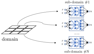
Figure 1: Cartoon illustrating domain decomposition and local random-weight neural networks.

We devise numerical algorithms to compute a least squares solution to the system (1) based on local randomized neural networks (or ELM). We decompose the domain $\Omega$ into sub-domains, and represent $u(\mathbf{x})$ on each sub-domain by a local ELM in a way analogous to in DongL2021 . Let $\Omega=\Omega_{1}\cup\Omega_{2}\cup\dots\cup\Omega_{N},$ where $\Omega_{i}$ ($1\leqslant i\leqslant N$) denote $N$ non-overlapping sub-domains (see Figure 1 for an illustration). Let

$$\small u(\mathbf{x})=\left\{\begin{array}[]{ll}u_{1}(\mathbf{x}),&\mathbf{x}\in\Omega_{1},\\ u_{2}(\mathbf{x}),&\mathbf{x}\in\Omega_{2},\\ \dots\\ u_{N}(\mathbf{x}),&\mathbf{x}\in\Omega_{N},\end{array}\right.$$ (2)

where $u_{i}(\mathbf{x})$ ($1\leqslant i\leqslant N$) denotes the solution field restricted to the sub-domain $\Omega_{i}$. On the interior sub-domain boundaries shared by adjacent sub-domains we impose $C^{\mathbf{k}}$ continuity conditions on $u(\mathbf{x})$, where $\mathbf{k}=(k_{1},\dots,k_{d})$ denotes a set of appropriate non-negative integers related to the order of the PDE (1a). If the PDE order (highest derivative) is $m_{i}$ along the $x_{i}$ ($1\leqslant i\leqslant d$) direction, we would in general impose $C^{m_{i}-1}$ (i.e. $k_{i}=m_{i}-1$) continuity conditions in this direction on the shared sub-domain boundaries.

On $\Omega_{i}$ ($1\leqslant i\leqslant N$) we employ a local FNN, whose hidden-layer coefficients are randomly assigned and fixed, to represent $u_{i}(\mathbf{x})$. More specifically, the local neural network is set as follows. The input layer consists of $d$ nodes, representing the input coordinate $\mathbf{x}=(x_{1},x_{2},\dots,x_{d})\in\Omega_{i}$. The output layer consists of a single node, representing $u_{i}(\mathbf{x})$. The network contains $(L-1)$ (with integer $L\geqslant 2$) hidden layers in between. Let $\sigma:\mathbb{R}\rightarrow\mathbb{R}$ denote the activation function for all the hidden nodes. Hereafter we use the following vector (or list) $\mathbf{M}$ of $(L+1)$ positive integers to represent the architecture of the local NN,

$$\small\mathbf{M}=\begin{bmatrix}m_{0},m_{1},\dots,m_{L-1},m_{L}\end{bmatrix},\quad\text{(architectural vector)}$$ (3)

where $m_{0}=d$ and $m_{L}=1$ denote the number of nodes in the input/output layers respectively, and $m_{i}$ is the number of nodes in the $i$-th hidden layer ($1\leqslant i\leqslant L-1$). We refer to $\mathbf{M}$ as an architectural vector.

We make the following assumptions:

• The output layer should contain (i) no bias, and (ii) no activation function (or equivalently, the activation function be $\sigma(x)=x$).

• The weights/biases in all the hidden layers are pre-set to uniform random values on $[-R_{m},R_{m}]$, where $R_{m}>0$ is a user-provided constant. The hidden-layer coefficients are fixed once they are set.

• The output-layer weights constitute the the trainable parameters of the local neural network.

We employ the same architecture, same activation function, and the same $R_{m}$ for the local neural networks on different sub-domains.

In light of these settings, the logic in the output layer of the local NNs leads to the following relation on the sub-domain $\Omega_{i}$ ($1\leqslant i\leqslant N$),

$$\small u_{i}(\mathbf{x})=\sum_{j=1}^{M}\beta_{ij}\phi_{ij}(\mathbf{x})=\bm{\Phi}_{i}(\mathbf{x})\bm{\beta}_{i},$$ (4)

where $M=m_{L-1}$ denotes the width of the last hidden layer of the local NN, $\phi_{ij}(\mathbf{x})$ ($1\leqslant j\leqslant M$) denote the set of output fields of the last hidden layer on $\Omega_{i}$, $\beta_{ij}$ ($1\leqslant j\leqslant M$) denote the set of output-layer coefficients (trainable parameters) on $\Omega_{i}$, and $\bm{\Phi}_{i}=(\phi_{i1},\phi_{i2},\dots,\phi_{iM})$ and $\bm{\beta}_{i}=(\beta_{i1},\beta_{i2},\dots,\beta_{iM})^{T}$. Note that, once the random hidden-layer coefficients are assigned, $\bm{\Phi}_{i}(\mathbf{x})$ in (4) denotes a set of random (but fixed and known) nonlinear basis functions. Therefore, with local ELMs the output field on each sub-domain is represented by an expansion of a set of random basis functions as given by (4).

With domain decomposition and local ELMs, the system (1) is symbolically transformed into the following form, which includes the continuity conditions across shared sub-domain boundaries:

$$\alpha_{1}\mathcal{L}_{1}(u_{i})+\alpha_{2}\mathcal{L}_{2}(u_{i})+\dots+\alpha_{n}\mathcal{L}_{n}(u_{i})+\mathcal{F}(u_{i})=f(\mathbf{x}),\quad\mathbf{x}\in\Omega_{i},\ 1\leqslant i\leqslant N;$$ (5a)

$$\mathcal{B}u_{i}(\mathbf{x})=g(\mathbf{x}),\quad\mathbf{x}\in\partial\Omega\cap\Omega_{i},\ 1\leqslant i\leqslant N;$$ (5b)

$$\mathcal{M}u_{i}(\bm{\xi})=S(\bm{\xi}),\quad\bm{\xi}\in\Omega_{s}\cap\Omega_{i},\ 1\leqslant i\leqslant N;$$ (5c)

$$\mathcal{C}u_{i}(\mathbf{x})-\mathcal{C}u_{j}(\mathbf{x})=0,\quad\mathbf{x}\in\partial\Omega_{i}\cap\partial\Omega_{j},\ \text{for all adjacent sub-domains}\ (\Omega_{i},\Omega_{j}),\ \ 1\leqslant i,j\leqslant N.$$ (5d)

In this system $u_{i}(\mathbf{x})$ is given by (4), and the operator $\mathcal{C}u$ denotes the set of $C^{\mathbf{k}}$ continuity conditions imposed across the shared sub-domain boundaries on $u$ or its derivatives. Define the residual of this system as,

$$\small\mathbf{R}(\bm{\alpha},\bm{\beta},\mathbf{x},\bm{\xi})=\begin{bmatrix}\alpha_{1}\mathcal{L}_{1}(u_{i})+\alpha_{2}\mathcal{L}_{2}(u_{i})+\dots+\alpha_{n}\mathcal{L}_{n}(u_{i})+\mathcal{F}(u_{i})-f(\mathbf{x}),\ \mathbf{x}\in\Omega_{i},\ 1\leqslant i\leqslant N\\ \mathcal{B}u_{i}(\mathbf{x})-g(\mathbf{x}),\ \mathbf{x}\in\partial\Omega\cap\Omega_{i},\ 1\leqslant i\leqslant N\\ \mathcal{M}u_{i}(\bm{\xi})-S(\bm{\xi}),\ \bm{\xi}\in\Omega_{s}\cap\Omega_{i},\ 1\leqslant i\leqslant N\\ \mathcal{C}u_{i}(\mathbf{x})-\mathcal{C}u_{j}(\mathbf{x}),\ \mathbf{x}\in\partial\Omega_{i}\cap\partial\Omega_{j},\ \text{for all adjacent}\ (\Omega_{i},\Omega_{j}),\ 1\leqslant i,j\leqslant N\end{bmatrix},$$ (6)

where $\bm{\beta}$ is the vector of all trainable parameters, $\bm{\beta}=(\bm{\beta}_{1}^{T},\dots,\bm{\beta}_{N}^{T})^{T}=(\beta_{11},\beta_{12},\dots,\beta_{1M},\beta_{21},\dots,\beta_{NM})^{T}$.

The system (5) is what we would solve numerically by least squares for the inverse parameters $\bm{\alpha}$ and the trainable network parameters $\bm{\beta}$. After $(\bm{\alpha},\bm{\beta})$ are determined, the field solution $u(\mathbf{x})$ is computed by (2) and (4). In what follows we present three algorithms, one based on the nonlinear least squares method with perturbations and the other two based on the variable projection idea, for determining the $\bm{\alpha}$ and $\bm{\beta}$.

2.2 Nonlinear Least Squares (NLLSQ) Method for Network Training

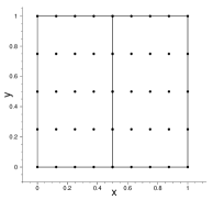
(a)   (b)

Figure 2: Sub-domains and collocation points: (a) Sketch of adjacent sub-domains. (b) Sketch of uniform grid points as collocation points ($5\times 5$ here) on two adjacent sub-domains.

We first outline a basic algorithm for computing $(\bm{\alpha},\bm{\beta})$ by the nonlinear least squares (NLLSQ) method with perturbations DongL2021 . It forms the basis for the variable projection algorithms presented in the next subsection.

For the simplicity of presentation we focus on rectangular domains, i.e. $\Omega=[a_{1},b_{1}]\times[a_{2},b_{2}]\times\dots\times[a_{d},b_{d}]$, where $a_{i}$ and $b_{i}$ ($1\leqslant i\leqslant d$) denote the lower/upper bounds of $\Omega$ in the $x_{i}$ direction, and assume that $\Omega$ is partitioned into $N_{i}$ ($N_{i}\geqslant 1$) sub-domains along $x_{i}$ ($1\leqslant i\leqslant d$).

To make the discussion more concrete, we specifically consider a second-order PDE in two dimensions ($d=2$, $\mathbf{x}=(x_{1},x_{2})=(x,y)$) as an example in this and the next subsections. In the following discussions we assume that equation (1a) is of second order with respect to both $x$ and $y$, and we impose $C^{1}$ continuity conditions across the sub-domain boundaries in both $x$ and $y$ directions.

Let the vectors $\bm{\mathcal{X}}=(X_{0},X_{1},\dots,X_{N_{1}})$ and $\bm{\mathcal{Y}}=(Y_{0},Y_{1},\dots,Y_{N_{2}})$ denote the sub-domain boundary points along the two directions, respectively, where $(X_{0},X_{N_{1}})=(a_{1},b_{1})$ and $(Y_{0},Y_{N_{2}})=(a_{2},b_{2})$. The total number of sub-domains is $N=N_{1}N_{2}$. We assume that the sub-domain $\Omega_{e}$ ($1\leqslant e\leqslant N$) is characterized by the partition indices $(i,j)$ along the $x$ and $y$ directions (see Figure 2(a)), with the following relation,

$$\small\begin{split}&\Omega_{e}=\Omega_{e(i,j)}=[X_{i-1},X_{i}]\times[Y_{j-1},Y_{j}],\quad e=e(i,j)=(i-1)N_{2}+j,\ \ \text{for}\ 1\leqslant(i,j)\leqslant(N_{1},N_{2}),\end{split}$$ (7)

where “$1\leqslant(i,j)\leqslant(N_{1},N_{2})$” or “$(1,1)\leqslant(i,j)\leqslant(N_{1},N_{2})$” stands for $1\leqslant i\leqslant N_{1}$ and $1\leqslant j\leqslant N_{2}$. We will use this and similar notations hereafter for conciseness.

With these settings the boundary conditions in (5b) are reduced to,

$$\mathcal{B}u_{e(1,j)}(a_{1},y)=g(a_{1},y),\quad\mathcal{B}u_{e(N_{1},j)}(b_{1},y)=g(b_{1},y),\quad\text{for}\ 1\leqslant j\leqslant N_{2};$$ (8a)

$$\mathcal{B}u_{e(i,1)}(x,a_{2})=g(x,a_{2}),\quad\mathcal{B}u_{e(i,N_{2})}(x,b_{2})=g(x,b_{2}),\quad\text{for}\ 1\leqslant i\leqslant N_{1}.$$ (8b)

Here $u_{e(i,j)}$ denotes $u$ on $\Omega_{e(i,j)}$, and $e(i,j)$ is given by (7). The $C^{1}$ continuity conditions in (5d) reduce to,

$$u_{e(i,j)}(X_{i},y)-u_{e(i+1,j)}(X_{i},y)=0,\quad\text{for}\ 1\leqslant(i,j)\leqslant(N_{1}-1,N_{2});$$ (9a)

$$\left.\frac{\partial u_{e(i,j)}}{\partial x}\right|_{(X_{i},y)}-\left.\frac{\partial u_{e(i+1,j)}}{\partial x}\right|_{(X_{i},y)}=0,\quad\text{for}\ 1\leqslant(i,j)\leqslant(N_{1}-1,N_{2});$$ (9b)

$$u_{e(i,j)}(x,Y_{j})-u_{e(i,j+1)}(x,Y_{j})=0,\quad\text{for}\ 1\leqslant(i,j)\leqslant(N_{1},N_{2}-1);$$ (9c)

$$\left.\frac{\partial u_{e(i,j)}}{\partial y}\right|_{(x,Y_{j})}-\left.\frac{\partial u_{e(i,j+1)}}{\partial y}\right|_{(x,Y_{j})}=0,\quad\text{for}\ 1\leqslant(i,j)\leqslant(N_{1},N_{2}-1).$$ (9d)

The equations (9a) and (9c) are the $C^{0}$ conditions on the horizontal/vertical sub-domain boundaries, and the equations (9b) and (9d) are the corresponding $C^{1}$ conditions.

The system to solve now consists of equations (5a), (8), (5c), and (9). This is a continuous system. We next enforce this system on a set of collocation points and measurement points to arrive at a discrete system about the parameters $\bm{\alpha}$ and $\bm{\beta}$.

We choose a set of $Q$ ($Q\geqslant 1$) collocation points on each sub-domain $\Omega_{e}$ ($1\leqslant e\leqslant N$), denoted by $\mathbf{x}_{p}^{e}=(x_{p}^{e},y_{p}^{e})$ ($1\leqslant p\leqslant Q$), among which $Q_{b}$ ($1\leqslant Q_{b}<Q$) points reside on $\partial\Omega_{e}$. Let $\mathbb{X}_{e}$ denote the set of collocation points on $\Omega_{e}$, and $\mathbb{X}_{e}^{b}=\mathbb{X}_{e}\cap\partial\Omega_{e}$ denote the set of collocation points residing on the sub-domain boundaries. The boundary collocation points on adjacent sub-domains are required to be compatible. That is, for any two adjacent sub-domains $(\Omega_{e_{1}},\Omega_{e_{2}})$, those boundary collocation points from $\Omega_{e_{1}}$ that reside on the shared boundary $\partial\Omega_{e_{1}}\cap\partial\Omega_{e_{2}}$ are required to be identical to those boundary collocation points from $\Omega_{e_{2}}$ that reside on the same boundary.

The collocation points can in principle be chosen based on various distributions (e.g. random, uniform). In this paper we focus on using uniform grid points as the collocation points; see Figure 2(b) for an illustration with a $5\times 5$ uniform grid points as the collocation points on two neighboring sub-domains. Let $Q_{1}$ and $Q_{2}$ denote the number of uniform grid points along $x$ and $y$, with $Q=Q_{1}Q_{2}$. The uniform collocation points on the sub-domain $\Omega_{e}=\Omega_{e(m,l)}$ ($1\leqslant(m,l)\leqslant(N_{1},N_{2})$) are given by

$$\footnotesize\left\{\begin{split}&\mathbf{x}_{p}^{e}=\mathbf{x}_{p(i,j)}^{e(m,l)}=\left(x_{p(i,j)}^{e(m,l)},y_{p(i,j)}^{e(m,l)}\right),\quad x_{p(i,j)}^{e(m,l)}=X_{m-1}+(i-1)(X_{m}-X_{m-1})/(Q_{1}-1),\\ &y_{p(i,j)}^{e(m,l)}=Y_{l-1}+(j-1)(Y_{l}-Y_{l-1})/(Q_{2}-1),\quad\text{for}\ 1\leqslant(m,l,i,j)\leqslant(N_{1},N_{2},Q_{1},Q_{2});\\ &p=p(i,j)=(i-1)Q_{2}+j,\quad\text{for}\ 1\leqslant(p,i,j)\leqslant(Q,Q_{1},Q_{2}).\end{split}\right.$$ (10)

We assume that the measurement data is given on a set of $Q_{s}$ ($Q_{s}\geqslant 1$) random measurement points (with a uniform distribution) on each $\Omega_{e}$ ($1\leqslant e\leqslant N$), denoted by $\bm{\xi}_{p}^{e}=(\xi_{p}^{e},\eta_{p}^{e})$ ($1\leqslant p\leqslant Q_{s}$). We use $\mathbb{Y}_{e}$ to denote the set of measurement points on $\Omega_{e}$ ($1\leqslant e\leqslant N$).

Once the hidden-layer coefficients of local NNs are randomly assigned and the collocation and measurement points are chosen, we compute the last hidden-layer field data $\bm{\Phi}_{e}(\mathbf{x}_{p}^{e})$ and their derivatives (up to a certain order), and the data for $\mathcal{M}\bm{\Phi}_{e}(\bm{\xi}_{p}^{e})$, by forward evaluations of the neural network and by auto-differtiations. We then store these data for subsequent use. In light of (4), for any given $\bm{\beta}=(\bm{\beta}_{1}^{T},\dots,\bm{\beta}_{N}^{T})^{T}$, we have

$$\small\begin{split}&u_{e}(\mathbf{x}_{p}^{e})=\bm{\Phi}_{e}(\mathbf{x}_{p}^{e})\bm{\beta}_{e},\ \mathcal{D}u_{e}(\mathbf{x}_{p}^{e})=\mathcal{D}\bm{\Phi}_{e}(\mathbf{x}_{p}^{e})\bm{\beta}_{e},\ \mathcal{M}u_{e}(\bm{\xi}_{q}^{e})=\mathcal{M}\bm{\Phi}_{e}(\bm{\xi}_{q}^{e})\bm{\beta}_{e},\ 1\leqslant(e,p,q)\leqslant(N,Q,Q_{s}),\end{split}$$ (11)

where $\mathcal{D}$ is a linear differential operator and $\mathcal{M}$ is the measurement operator.

Remark 2.2.

To compute $\bm{\Phi}_{e}(\mathbf{x}_{p}^{e})$, $\mathcal{D}\bm{\Phi}_{e}(\mathbf{x}_{p}^{e})$ and $\mathcal{M}\bm{\Phi}_{e}(\bm{\xi}_{p}^{e})$, in the implementation we create a Keras sub-model, referred to as the last-hidden-layer-model, to the local NN for each sub-domain. The input nodes to this sub-model are identical to those of the original local NN, and the output nodes of this sub-model consist of those nodes in the last hidden layer of the original local NN. We compute $\bm{\Phi}_{e}(\mathbf{x}_{p}^{e})$ ($1\leqslant p\leqslant Q$) and $\bm{\Phi}_{e}(\bm{\xi}_{p}^{e})$ ($1\leqslant p\leqslant Q_{s}$) by a forward evaluation of the last-hidden-layer-model for $\Omega_{e}$ on the input data (collocation points, or measurement points). We compute the derivatives of $\bm{\Phi}_{e}$ on $\mathbf{x}_{p}^{e}$ or on $\bm{\xi}_{p}^{e}$ by a forward-mode auto-differentiation of the last-hidden-layer-model, implemented by the “ForwardAccumulator” in the Tensorflow library. The forward-mode auto-differentiation is crucial to the performance of the ELM method (see DongY2022rm ).

To derive the discrete system we enforce (5a) on all the collocation points in $\mathbb{X}_{e}$ ($1\leqslant e\leqslant N$), enforce (8) on all the boundary collocation points in $\mathbb{X}_{e}^{b}\cap\partial\Omega$ for $1\leqslant e\leqslant N$, enforce (5c) on all the measurement points in $\mathbb{Y}_{e}$ ($1\leqslant e\leqslant N$), and enforce (9) on those collocation points from $\mathbb{X}_{e}^{b}$ ($1\leqslant e\leqslant N$) that reside on the shared boundaries of adjacent sub-domains.

The discrete system corresponding to (5a) enforced on the collocation points is,

$$\footnotesize\alpha_{1}\mathcal{L}_{1}\left(u_{e}(\mathbf{x}_{p}^{e})\right)+\dots+\alpha_{n}\mathcal{L}_{n}\left(u_{e}(\mathbf{x}_{p}^{e})\right)+\mathcal{F}\left(u_{e}(\mathbf{x}_{p}^{e})\right)-f\left(\mathbf{x}_{p}^{e}\right)=0,\ \text{for}\ \mathbf{x}_{p}^{e}\in\mathbb{X}_{e},\ 1\leqslant(e,p)\leqslant(N,Q).$$ (12)

The discrete system corresponding to (8) on the boundary collocation points is given by,

$$\mathcal{B}u_{e(1,l)}(a_{1},y_{p(1,j)}^{e(1,l)})-g(a_{1},y_{p(1,j)}^{e(1,l)})=0,\quad\text{for}\ 1\leqslant(l,j)\leqslant(N_{2},Q_{2});$$ (13a)

$$\mathcal{B}u_{e(N_{1},l)}(b_{1},y_{p(Q_{1},j)}^{e(N_{1},l)})-g(b_{1},y_{p(Q_{1},j)}^{e(N_{1},l)})=0,\quad\text{for}\ 1\leqslant(l,j)\leqslant(N_{2},Q_{2});$$ (13b)

$$\mathcal{B}u_{e(m,1)}(x_{p(i,1)}^{e(m,1)},a_{2})-g(x_{p(i,1)}^{e(m,1)},a_{2})=0,\quad\text{for}\ 1\leqslant(m,i)\leqslant(N_{1},Q_{1});$$ (13c)

$$\mathcal{B}u_{e(m,N_{2})}(x_{p(i,Q_{2})}^{e(m,N_{2})},b_{2})-g(x_{p(i,Q_{2})}^{e(m,N_{2})},b_{2})=0,\quad\text{for}\ 1\leqslant(m,i)\leqslant(N_{1},Q_{1}).$$ (13d)

Here the functions $e(\cdot,\cdot)$ and $p(\cdot,\cdot)$ are defined in (7) and (10), respectively. The discrete system corresponding to (5c) enforced on the measurement points is given by

$$\footnotesize\mathcal{M}u_{e}(\bm{\xi}_{p}^{e})-S(\bm{\xi}_{p}^{e})=0,\quad\text{for}\ \bm{\xi}_{p}^{e}\in\mathbb{Y}_{e},\ 1\leqslant(e,p)\leqslant(N,Q_{s}).$$ (14)

The discrete system corresponding to (9) enforced on the interior sub-domain boundary points is,

$$u_{e(m,l)}(X_{m},y_{p(Q_{1},j)}^{e(m,l)})-u_{e(m+1,l)}(X_{m},y_{p(1,j)}^{e(m+1,l)})=0,\quad\text{for}\ 1\leqslant(m,l,j)\leqslant(N_{1}-1,N_{2},Q_{2});$$ (15a)

$$\left.\frac{\partial u_{e(m,l)}}{\partial x}\right|_{(X_{m},y_{p(Q_{1},j)}^{e(m,l)})}-\left.\frac{\partial u_{e(m+1,l)}}{\partial x}\right|_{(X_{m},y_{p(1,j)}^{e(m+1,l)})}=0,\quad\text{for}\ 1\leqslant(m,l,j)\leqslant(N_{1}-1,N_{2},Q_{2});$$ (15b)

$$u_{e(m,l)}(x_{p(i,Q_{2})}^{e(m,l)},Y_{l})-u_{e(m,l+1)}(x_{p(i,1)}^{e(m,l+1)},Y_{l})=0,\quad\text{for}\ 1\leqslant(m,l,i)\leqslant(N_{1},N_{2}-1,Q_{1});$$ (15c)

$$\left.\frac{\partial u_{e(m,l)}}{\partial y}\right|_{(x_{p(i,Q_{2})}^{e(m,l)},Y_{l})}-\left.\frac{\partial u_{e(m,l+1)}}{\partial y}\right|_{(x_{p(i,1)}^{e(m,l+1)},Y_{l})}=0,\quad\text{for}\ 1\leqslant(m,l,i)\leqslant(N_{1},N_{2}-1,Q_{1}).$$ (15d)

In the above equations $\mathbf{x}_{p}^{e}$, $x_{p(i,j)}^{e(m,l)}$ and $y_{p(i,j)}^{e(m,l)}$ are defined in (10), and $u_{e}(\mathbf{x})$ is given by (4) and (11).

The equations (12)–(15d) form the system we would solve to determine the inverse parameters $\bm{\alpha}=(\alpha_{1},\dots,\alpha_{n})^{T}$ and the trainable network parameters $\bm{\beta}=(\beta_{11},\dots,\beta_{NM})^{T}$. This is a system of nonlinear algebraic equations about ($\bm{\alpha}$, $\bm{\beta}$). Note that the functions $\bm{\Phi}_{e}(\mathbf{x})$ ($1\leqslant e\leqslant N$) and their derivatives evaluated on the collocation/measurement points, which are involved in the operators such as $\mathcal{L}_{i}(u_{e})$, $\mathcal{F}(u_{e})$, $\mathcal{B}u_{e}$, $\mathcal{M}u_{e}$, and $\mathcal{C}u_{e}$, are computed by evaluations of the neural network and auto-differentiations (see Remark 2.2). This system consists of $N_{c}$ equations and a total of $N_{a}$ unknowns, where

$$\small N_{c}=N(Q+Q_{s}+2Q_{1}+2Q_{2}),\quad N_{a}=N_{L}+n=NM+n,$$ (16)

and $N_{L}=NM$ is the total number of trainable parameters in the neural network.

We seek a least squares solution to this system, and solve this system for $(\bm{\alpha},\bm{\beta})$ by the nonlinear least squares (NLLSQ) method Bjorck1996 ; DongL2021 . In our implementation we take advantage of the quality implementations of the nonlinear least squares method in the scientific libraries, specficially the “least_squares()” routine from the scipy.optimize package in Python for the current work. This library routine implements the Gauss-Newton method Bjorck1996 together with a trust region algorithm BranchCL1999 ; ByrdSS1988 .

Since the nonlinear least squares method is a local optimization algorithm, it can be trapped to a local-minimum solution that is unacceptable. It is therefore crucial to combine the nonlinear least squares method with some perturbation strategy when solving the nonlinear least squares problem, in order to prevent the method from being trapped to the worst local-minimum solutions. In this paper we adopt the strategy for the initial guess perturbation and sub-iteration procedure developed in DongL2021 , with some modifications, and combine it with the nonlinear least squares method for solving the current system arising from the inverse PDE problem. We refer to the combined algorithm as the nonlinear least squares method with perturbations (NLLSQ-perturb). The NLLSQ-perturb algorithm is listed in the Appendix A of this paper (as Algorithm 7), which contains explanations of the various input parameters to the algorithm.

The NLLSQ-perturb algorithm (Algorithm 7) requires two routines, one for computing the residual vector and the other for computing the Jacobian matrix for an arbitrary given approximation to the solution. When the system (5) is enforced on the collocation points, the residual function in (6) is reduced to the vector,

$$\footnotesize\mathbf{R}(\bm{\alpha},\bm{\beta})=\begin{bmatrix}\mathbf{R}^{\text{pde}}(\bm{\alpha},\bm{\beta})\\ \mathbf{R}^{\text{bc}}(\bm{\beta})\\ \mathbf{R}^{\text{mea}}(\bm{\beta})\\ \mathbf{R}^{\text{ck}}(\bm{\beta})\end{bmatrix}_{N_{c}\times 1}.$$ (17)

In this expression,

$$\footnotesize\left\{\begin{split}&\mathbf{R}^{\text{pde}}=\begin{bmatrix}\vdots\\ R^{\text{pde}}_{ep}\\ \vdots\end{bmatrix}_{NQ\times 1};\ \mathbf{R}^{\text{mea}}=\begin{bmatrix}\vdots\\ R^{\text{mea}}_{ep}\\ \vdots\end{bmatrix}_{NQ_{s}\times 1};\ \mathbf{R}^{\text{bc}}=\begin{bmatrix}\mathbf{R}^{\text{bc1}}\\ \mathbf{R}^{\text{bc2}}\\ \mathbf{R}^{\text{bc3}}\\ \mathbf{R}^{\text{bc4}}\end{bmatrix};\ \mathbf{R}^{\text{ck}}=\begin{bmatrix}\mathbf{R}^{\text{ck1}}\\ \mathbf{R}^{\text{ck2}}\\ \mathbf{R}^{\text{ck3}}\\ \mathbf{R}^{\text{ck4}}\end{bmatrix};\ \mathbf{R}^{\text{bc1}}=\begin{bmatrix}\vdots\\ R_{lj}^{bc1}\\ \vdots\end{bmatrix}_{N_{2}Q_{2}\times 1},\\ &\mathbf{R}^{\text{bc2}}=\begin{bmatrix}\vdots\\ R_{lj}^{bc2}\\ \vdots\end{bmatrix}_{N_{2}Q_{2}\times 1},\ \mathbf{R}^{\text{bc3}}=\begin{bmatrix}\vdots\\ R_{mi}^{bc3}\\ \vdots\end{bmatrix}_{N_{1}Q_{1}\times 1},\ \mathbf{R}^{\text{bc4}}=\begin{bmatrix}\vdots\\ R_{mi}^{bc4}\\ \vdots\end{bmatrix}_{N_{1}Q_{1}\times 1};\ \mathbf{R}^{\text{ck1}}=\begin{bmatrix}\vdots\\ R_{mlj}^{ck1}\\ \vdots\end{bmatrix}_{(N-N_{2})Q_{2}\times 1},\\ &\mathbf{R}^{\text{ck2}}=\begin{bmatrix}\vdots\\ R_{mlj}^{ck2}\\ \vdots\end{bmatrix}_{(N-N_{2})Q_{2}\times 1},\ \mathbf{R}^{\text{ck3}}=\begin{bmatrix}\vdots\\ R_{mli}^{ck3}\\ \vdots\end{bmatrix}_{(N-N_{1})Q_{1}\times 1},\ \mathbf{R}^{\text{ck4}}=\begin{bmatrix}\vdots\\ R_{mli}^{ck4}\\ \vdots\end{bmatrix}_{(N-N_{1})Q_{1}\times 1}.\end{split}\right.$$ (18)

In the above expressions, $R^{\text{pde}}_{ep}$ is the left hand side (LHS) of (12), and $R^{\text{mea}}_{ep}$ is the LHS of (14). $R_{lj}^{bc1}$, $R_{lj}^{bc2}$, $R_{mi}^{bc3}$ and $R_{mi}^{bc4}$ are the LHSs of (13a)–(13d), respectively. $R_{mlj}^{ck1}$, $R_{mlj}^{ck2}$, $R_{mli}^{ck3}$ and $R_{mli}^{ck4}$ are the LHSs of (15a)–(15d), respectively.

We therefore compute the residual vector $\mathbf{R}(\bm{\alpha},\bm{\beta})$ as follows. Given arbitrary $(\bm{\alpha},\bm{\beta})$, we compute $u_{e}(\mathbf{x}_{p}^{e})$ ($\mathbf{x}_{p}^{e}\in\mathbb{X}_{e}$) for $1\leqslant e\leqslant N$, and their derivatives by (11). Then we compute the LHSs of the equations (12), (13a)–(13d), (14), and (15a)–(15d), and assemble them to form the vectors $\mathbf{R}^{\text{pde}}$, $\mathbf{R}^{\text{bc}}$, $\mathbf{R}^{\text{mea}}$ and $\mathbf{R}^{\text{ck}}$. The residual vector $\mathbf{R}(\bm{\alpha},\bm{\beta})$ is finally assembled according to (17). The procedure for computing $\mathbf{R}(\bm{\alpha},\bm{\beta})$ is summarized in Algorithm 1.

1

input :  vector $\bm{\theta}=(\bm{\alpha},\bm{\beta})$; $\bm{\Phi}_{e}(x_{p}^{e})$ and derivatives $(1\leqslant(e,p)\leqslant(N,Q))$; $\mathcal{M}\bm{\Phi}_{e}(\bm{\xi}_{p}^{e})$ $(1\leqslant(e,p)\leqslant(N,Q_{s}))$.

output : residual vector $\mathbf{R}(\bm{\theta})$

2 if $\bm{\theta}=\bm{\theta}_{s}$ then

3       retrieve $u_{e}(\mathbf{x}_{p}^{e})$ $(1\leqslant(e,p)\leqslant(N,Q))$ and their derivatives, and $\mathcal{M}u_{e}(\bm{\xi}_{p}^{e})$ $(1\leqslant(e,p)\leqslant(N,Q_{s}))$

4      

5else

6       compute $u_{e}(\mathbf{x}_{p}^{e})$ $(1\leqslant(e,p)\leqslant(N,Q))$, their derivatives (up to a necessary order), and $\mathcal{M}u_{e}(\bm{\xi}_{p}^{e})$ $(1\leqslant(e,p)\leqslant(N,Q_{s}))$ by (11)

7       set $\bm{\theta}_{s}=\bm{\theta}$, and save $u_{e}(\mathbf{x}_{p}^{e})$ $(1\leqslant(e,p)\leqslant(N,Q))$, their derivatives, and $\mathcal{M}u_{e}(\bm{\xi}_{p}^{e})$ $(1\leqslant(e,p)\leqslant(N,Q_{s}))$

8      

9 end if

10compute $\mathbf{R}^{\text{pde}}(\bm{\theta})$, $\mathbf{R}^{\text{bc}}(\bm{\theta})$, $\mathbf{R}^{\text{mea}}(\bm{\theta})$, $\mathbf{R}^{\text{ck}}(\bm{\theta})$ by the LHSs of (12)–(15d), respectively

11 form $\mathbf{R}(\bm{\theta})$ according to (17)

12

Algorithm 1 Computing the residual $\mathbf{R}(\bm{\alpha},\bm{\beta})$ for NLLSQ algorithm

Remark 2.3.

On line $4$ of Algorithm 1, the “necessary order” refers to the order of all the derivative terms of $u_{e}$ involved in the system consisting of (12)–(15d). For example, if $\frac{\partial^{2}u_{e}}{\partial y^{2}}$ and $\frac{\partial u_{e}}{\partial x}$ are involved in this system, one would need to compute these derivatives based on $\frac{\partial^{2}\bm{\Phi}_{e}}{\partial y^{2}}$ and $\frac{\partial\bm{\Phi}_{e}}{\partial x}$ on line $4$ of this algorithm.

The Jacobian matrix is given by

$$\footnotesize\frac{\partial\mathbf{R}}{\partial(\bm{\alpha},\bm{\beta})}=\begin{bmatrix}\frac{\partial\mathbf{R}}{\partial\bm{\alpha}}&\frac{\partial\mathbf{R}}{\partial\bm{\beta}}\end{bmatrix}=\begin{bmatrix}\frac{\partial\mathbf{R}^{\text{pde}}}{\partial\bm{\alpha}}&\frac{\partial\mathbf{R}^{\text{pde}}}{\partial\bm{\beta}}\\ \mathbf{0}&\frac{\partial\mathbf{R}^{\text{bc}}}{\partial\bm{\beta}}\\ \mathbf{0}&\frac{\partial\mathbf{R}^{\text{mea}}}{\partial\bm{\beta}}\\ \mathbf{0}&\frac{\partial\mathbf{R}^{\text{ck}}}{\partial\bm{\beta}}\end{bmatrix}_{N_{c}\times N_{L}}.$$ (19)

In this expression,

$$\footnotesize\left\{\begin{split}&\frac{\partial\mathbf{R}^{\text{pde}}}{\partial\bm{\alpha}}=\begin{bmatrix}\frac{\partial R_{ep}^{\text{pde}}}{\partial\alpha_{i}}\end{bmatrix}_{NQ\times n}=\begin{bmatrix}\mathcal{L}_{1}(u_{e}(\mathbf{x}_{p}^{e}))&\dots&\mathcal{L}_{n}(u_{e}(\mathbf{x}_{p}^{e}))\end{bmatrix}_{NQ\times n},\ \frac{\partial\mathbf{R}^{\text{pde}}}{\partial\bm{\beta}}=\begin{bmatrix}\frac{\partial R_{ep}^{\text{pde}}}{\partial\beta_{ij}}\end{bmatrix}_{NQ\times NM},\\ &\frac{\partial\mathbf{R}^{\text{mea}}}{\partial\bm{\beta}}=\begin{bmatrix}\frac{\partial R_{ep}^{\text{mea}}}{\partial\beta_{ij}}\end{bmatrix}_{NQ_{s}\times NM},\frac{\partial\mathbf{R}^{\text{bc}}}{\partial\bm{\beta}}=\begin{bmatrix}\frac{\partial\mathbf{R}^{\text{bc1}}}{\partial\bm{\beta}}\\ \frac{\partial\mathbf{R}^{\text{bc2}}}{\partial\bm{\beta}}\\ \frac{\partial\mathbf{R}^{\text{bc3}}}{\partial\bm{\beta}}\\ \frac{\partial\mathbf{R}^{\text{bc4}}}{\partial\bm{\beta}}\end{bmatrix},\ \frac{\partial\mathbf{R}^{\text{ck}}}{\partial\bm{\beta}}=\begin{bmatrix}\frac{\partial\mathbf{R}^{\text{ck1}}}{\partial\bm{\beta}}\\ \frac{\partial\mathbf{R}^{\text{ck2}}}{\partial\bm{\beta}}\\ \frac{\partial\mathbf{R}^{\text{ck3}}}{\partial\bm{\beta}}\\ \frac{\partial\mathbf{R}^{\text{ck4}}}{\partial\bm{\beta}}\end{bmatrix},\ \frac{\partial\mathbf{R}^{\text{bc1}}}{\partial\bm{\beta}}=\begin{bmatrix}\frac{\partial R_{lj}^{\text{bc1}}}{\partial\beta_{ik}}\end{bmatrix}_{N_{2}Q_{2}\times NM},\\ &\frac{\partial\mathbf{R}^{\text{bc2}}}{\partial\bm{\beta}}=\begin{bmatrix}\frac{\partial R_{lj}^{\text{bc2}}}{\partial\beta_{ik}}\end{bmatrix}_{N_{2}Q_{2}\times NM},\ \frac{\partial\mathbf{R}^{\text{bc3}}}{\partial\bm{\beta}}=\begin{bmatrix}\frac{\partial R_{mi}^{\text{bc3}}}{\partial\beta_{lk}}\end{bmatrix}_{N_{1}Q_{1}\times NM},\frac{\partial\mathbf{R}^{\text{bc4}}}{\partial\bm{\beta}}=\begin{bmatrix}\frac{\partial R_{mi}^{\text{bc4}}}{\partial\beta_{lk}}\end{bmatrix}_{N_{1}Q_{1}\times NM},\\ &\frac{\partial\mathbf{R}^{\text{ck1}}}{\partial\bm{\beta}}=\begin{bmatrix}\frac{\partial R_{mlj}^{\text{ck1}}}{\partial\beta_{iq}}\end{bmatrix}_{(N-N_{2})Q_{2}\times NM},\ \frac{\partial\mathbf{R}^{\text{ck2}}}{\partial\bm{\beta}}=\begin{bmatrix}\frac{\partial R_{mlj}^{\text{ck2}}}{\partial\beta_{iq}}\end{bmatrix}_{(N-N_{2})Q_{2}\times NM},\ \frac{\partial\mathbf{R}^{\text{ck3}}}{\partial\bm{\beta}}=\begin{bmatrix}\frac{\partial R_{mli}^{\text{ck3}}}{\partial\beta_{jq}}\end{bmatrix}_{(N-N_{1})Q_{1}\times NM},\\ &\frac{\partial\mathbf{R}^{\text{ck4}}}{\partial\bm{\beta}}=\begin{bmatrix}\frac{\partial R_{mli}^{\text{ck4}}}{\partial\beta_{jq}}\end{bmatrix}_{(N-N_{1})Q_{1}\times NM}.\end{split}\right.$$ (20)

In the matrix $\frac{\partial\mathbf{R}^{\text{pde}}}{\partial\bm{\beta}}$ the only non-zero terms are

$$\footnotesize\frac{\partial R_{ep}^{\text{pde}}}{\partial\beta_{ej}}=\alpha_{1}\mathcal{L}_{1}^{\prime}(u_{e}(\mathbf{x}_{p}^{e}))\phi_{ej}(\mathbf{x}_{p}^{e})+\dots+\alpha_{n}\mathcal{L}_{n}^{\prime}(u_{e}(\mathbf{x}_{p}^{e}))\phi_{ej}(\mathbf{x}_{p}^{e})+\mathcal{F}^{\prime}(u_{e}(\mathbf{x}_{p}^{e}))\phi_{ej}(\mathbf{x}_{p}^{e}),\\ \text{for}\ 1\leqslant(e,p,j)\leqslant(N,Q,M),$$ (21)

where $\mathcal{L}_{i}^{\prime}(u)$ ($1\leqslant i\leqslant n$) denote the derivatives of $\mathcal{L}_{i}(u)$ with respect to $u$, and $\mathcal{F}^{\prime}(u)$ denotes the derivative of $\mathcal{F}(u)$ with respect to $u$. In the matrix $\frac{\partial\mathbf{R}^{\text{mea}}}{\partial\bm{\beta}}$ the only non-zero terms are

$$\footnotesize\frac{\partial R_{ep}^{\text{mea}}}{\partial\beta_{ej}}=\mathcal{M}\phi_{ej}(\bm{\xi}_{p}^{e}),\quad\text{for}\ 1\leqslant(e,p,j)\leqslant(N,Q_{s},M).$$ (22)

In the matrices $\frac{\partial\mathbf{R}^{\text{bc1}}}{\partial\bm{\beta}}$, $\frac{\partial\mathbf{R}^{\text{bc2}}}{\partial\bm{\beta}}$, $\frac{\partial\mathbf{R}^{\text{bc3}}}{\partial\bm{\beta}}$ and $\frac{\partial\mathbf{R}^{\text{bc4}}}{\partial\bm{\beta}}$ the only non-zero terms are,

$$\footnotesize\left\{\begin{split}&\frac{\partial R_{lj}^{\text{bc1}}}{\partial\beta_{lq}}=\mathcal{B}\phi_{eq}(a_{1},y_{p}^{e}),\ \text{where}\ e=e(1,l),\ p=p(1,j),\quad\text{for}\ 1\leqslant(l,j,q)\leqslant(N_{2},Q_{2},M);\\ &\frac{\partial R_{lj}^{\text{bc2}}}{\partial\beta_{lq}}=\mathcal{B}\phi_{eq}(b_{1},y_{p}^{e}),\ \text{where}\ e=e(N_{1},l),\ p=p(Q_{1},j),\quad\text{for}\ 1\leqslant(l,j,q)\leqslant(N_{2},Q_{2},M);\\ &\frac{\partial R_{mi}^{\text{bc3}}}{\partial\beta_{mq}}=\mathcal{B}\phi_{eq}(x_{p}^{e},a_{2}),\ \text{where}\ e=e(m,1),\ p=p(i,1),\quad\text{for}\ 1\leqslant(m,i,q)\leqslant(N_{1},Q_{1},M);\\ &\frac{\partial R_{mi}^{\text{bc4}}}{\partial\beta_{mq}}=\mathcal{B}\phi_{eq}(x_{p}^{e},b_{2}),\ \text{where}\ e=e(m,N_{2}),\ p=p(i,Q_{2}),\quad\text{for}\ 1\leqslant(m,i,q)\leqslant(N_{1},Q_{1},M).\end{split}\right.$$ (23)

In the matrices $\frac{\partial\mathbf{R}^{\text{ck1}}}{\partial\bm{\beta}}$, $\frac{\partial\mathbf{R}^{\text{ck2}}}{\partial\bm{\beta}}$, $\frac{\partial\mathbf{R}^{\text{ck3}}}{\partial\bm{\beta}}$ and $\frac{\partial\mathbf{R}^{\text{ck4}}}{\partial\bm{\beta}}$ the only non-zero terms are,

$$\footnotesize\left\{\begin{split}&\frac{\partial R_{mlj}^{\text{ck1}}}{\partial\beta_{e_{1}q}}=\phi_{e_{1}q}(X_{m},y_{p_{1}}^{e_{1}}),\quad\frac{\partial R_{mlj}^{\text{ck1}}}{\partial\beta_{e_{2}q}}=-\phi_{e_{2}q}(X_{m},y_{p_{2}}^{e_{2}}),\quad\text{where}\ e_{1}=e(m,l),\ e_{2}=e(m+1,l),\\ &\qquad\qquad\qquad\qquad p_{1}=p(Q_{1},j),\ p_{2}=p(1,j),\ \text{for}\ 1\leqslant(m,l,j,q)\leqslant(N_{1}-1,N_{2},Q_{2},M);\\ &\frac{\partial R_{mlj}^{\text{ck2}}}{\partial\beta_{e_{1}q}}=\left.\frac{\partial\phi_{e_{1}q}}{\partial x}\right|_{(X_{m},y_{p_{1}}^{e_{1}})},\quad\frac{\partial R_{mlj}^{\text{ck2}}}{\partial\beta_{e_{2}q}}=-\left.\frac{\partial\phi_{e_{2}q}}{\partial x}\right|_{(X_{m},y_{p_{2}}^{e_{2}})},\ \text{where}\ e_{1}=e(m,l),\ e_{2}=e(m+1,l),\\ &\qquad\qquad\qquad\qquad p_{1}=p(Q_{1},j),\ p_{2}=p(1,j),\ \text{for}\ 1\leqslant(m,l,j,q)\leqslant(N_{1}-1,N_{2},Q_{2},M);\\ &\frac{\partial R_{mli}^{\text{ck3}}}{\partial\beta_{e_{1}q}}=\phi_{e_{1}q}(x_{p_{1}}^{e_{1}},Y_{l}),\quad\frac{\partial R_{mli}^{\text{ck3}}}{\partial\beta_{e_{2}q}}=-\phi_{e_{2}q}(x_{p_{2}}^{e_{2}},Y_{l}),\quad\text{where}\ e_{1}=e(m,l),\ e_{2}=e(m,l+1),\\ &\qquad\qquad\qquad\qquad p_{1}=p(i,Q_{2}),\ p_{2}=p(i,1),\ \text{for}\ 1\leqslant(m,l,i,q)\leqslant(N_{1},N_{2}-1,Q_{1},M);\\ &\frac{\partial R_{mli}^{\text{ck4}}}{\partial\beta_{e_{1}q}}=\left.\frac{\partial\phi_{e_{1}q}}{\partial y}\right|_{(x_{p_{1}}^{e_{1}},Y_{l})},\quad\frac{\partial R_{mli}^{\text{ck4}}}{\partial\beta_{e_{2}q}}=-\left.\frac{\partial\phi_{e_{2}q}}{\partial y}\right|_{(x_{p_{2}}^{e_{2}},Y_{l})},\ \text{where}\ e_{1}=e(m,l),\ e_{2}=e(m,l+1),\\ &\qquad\qquad\qquad\qquad p_{1}=p(i,Q_{2}),\ p_{2}=p(i,1),\ \text{for}\ 1\leqslant(m,l,i,q)\leqslant(N_{1},N_{2}-1,Q_{1},M).\end{split}\right.$$ (24)

Therefore the Jacobian matrix can be computed as follows. Given arbitrary $(\bm{\alpha},\bm{\beta})$, we compute $u_{e}(\mathbf{x}_{p}^{e})$ ($1\leqslant(e,p)\leqslant(N,Q)$), their derivatives, and $\mathcal{M}u_{e}(\bm{\xi}_{p}^{e})$ ($1\leqslant(e,p)\leqslant(N,Q_{s})$) based on $\bm{\beta}$ and the pre-computed $\bm{\Phi}_{e}(\mathbf{x}_{p}^{e})$, their derivatives, and the $\mathcal{M}\bm{\Phi}_{e}(\bm{\xi}_{p}^{e})$ data. Then we compute the Jacobian and related matrices by the equations (19)–(24). Algorithm 2 summarizes the routine for computing the Jacobian matrix.

1

input :  vector $\bm{\theta}=(\bm{\alpha},\bm{\beta})$; $\bm{\Phi}_{e}(x_{p}^{e})$ and derivatives $(1\leqslant(e,p)\leqslant(N,Q))$; $\mathcal{M}\bm{\Phi}_{e}(\bm{\xi}_{p}^{e})$ $(1\leqslant(e,p)\leqslant(N,Q_{s}))$.

output : Jacobian matrix $\frac{\partial\mathbf{R}}{\partial\bm{\theta}}$

2 if $\bm{\theta}=\bm{\theta}_{s}$ then

3       retrieve $u_{e}(\mathbf{x}_{p}^{e})$ $(1\leqslant(e,p)\leqslant(N,Q))$ and their derivatives, and $\mathcal{M}u_{e}(\bm{\xi}_{p}^{e})$ $(1\leqslant(e,p)\leqslant(N,Q_{s}))$

4      

5else

6       compute $u_{e}(\mathbf{x}_{p}^{e})$ $(1\leqslant(e,p)\leqslant(N,Q))$, their derivatives (up to a necessary order), and $\mathcal{M}u_{e}(\bm{\xi}_{p}^{e})$ $(1\leqslant(e,p)\leqslant(N,Q_{s}))$ by (11)

7       set $\bm{\theta}_{s}=\bm{\theta}$, and save $u_{e}(\mathbf{x}_{p}^{e})$ $(1\leqslant(e,p)\leqslant(N,Q))$, their derivatives, and $\mathcal{M}u_{e}(\bm{\xi}_{p}^{e})$ $(1\leqslant(e,p)\leqslant(N,Q_{s}))$

8      

9 end if

10compute $\frac{\partial\mathbf{R}^{\text{pde}}}{\partial\bm{\alpha}}$, $\frac{\partial\mathbf{R}^{\text{pde}}}{\partial\bm{\beta}}$, $\frac{\partial\mathbf{R}^{\text{bc}}}{\partial\bm{\beta}}$, $\frac{\partial\mathbf{R}^{\text{mea}}}{\partial\bm{\beta}}$, $\frac{\partial\mathbf{R}^{\text{ck}}}{\partial\bm{\beta}}$ by (20)–(24)

11 form $\frac{\partial\mathbf{R}}{\partial\bm{\theta}}=\frac{\partial\mathbf{R}}{\partial(\bm{\alpha},\bm{\beta})}$ by (19)

12

Algorithm 2 Computing the Jacobian matrix $\frac{\partial\mathbf{R}}{\partial(\bm{\alpha},\bm{\beta})}$ for NLLSQ algorithm

Remark 2.4.

In Algorithms 1 and 2 we have stored the data for $u$, its derivatives, and $\mathcal{M}u$ on the collocation/measurement points corresponding to the $\bm{\theta}=(\bm{\alpha},\bm{\beta})$ value last computed (denoted by $\bm{\theta}_{s}$); see lines $1$ to $6$ in both algorithms. This saves computations, because in the nonlinear least squares iterations Algorithm 1 is typically invoked first to compute the residual corresponding to some $(\bm{\alpha},\bm{\beta})$, and then Algorithm 2 is invoked to compute the Jacobian for the same $(\bm{\alpha},\bm{\beta})$.

Remark 2.5.

In this work the hidden-layer coefficients are assigned to uniform random values generated on the interval $[-R_{m},R_{m}]$, where $R_{m}>0$ is a constant. The $R_{m}$ value influences the accuracy of the simulation results of inverse PDE problems, similar to what has been observed in forward problems (see DongL2021 ; DongY2022rm ). In this paper we compute a near-optimal $R_{m}$ using the method from DongY2022rm based on the differential evolution algorithm, and employ this value (or a value nearby) in numerical simulations of inverse PDEs.

Remark 2.6.

For noisy measurement data $S(\bm{\xi})$, we observe that scaling the residual vector associated with the measurement ($\mathbf{R}^{\text{mea}}$) by a constant factor can improve the accuracy of the results (more robust to noise). Let $\lambda_{mea}>0$ denote a prescribed constant. We scale the equation (14) by $\lambda_{mea}$,

$$\footnotesize\lambda_{mea}\mathcal{M}u_{e}(\bm{\xi}_{p}^{e})-\lambda_{mea}S(\bm{\xi}_{p}^{e})=0,\quad\text{for}\ \bm{\xi}_{p}^{e}\in\mathbb{Y}_{e},\ 1\leqslant(e,p)\leqslant(N,Q_{s}).$$ (25)

Then in the presented method we replace equation (14) by the scaled equation (25), with corresponding changes to the computation of the residual vector and the Jacobian matrix. The scaling factor $\lambda_{mea}$ will cause some change to the least squares solution to ($\bm{\alpha},\bm{\beta}$). When the data $S(\bm{\xi})$ is noisy, numerical experiments indicate that employing a constant $0<\lambda_{mea}<1$ can in general improve the accuracy of the computed $\bm{\alpha}$ and $u(\mathbf{x})$ markedly, compared with the case without scaling (i.e. $\lambda_{mea}=1$). Note that employing the scaled equation (25) is equivalent to using a scaled term $\frac{1}{2}\lambda_{mea}^{2}\|\mathbf{R}^{\text{mea}}\|^{2}$ in the underlying loss function for the nonlinear least squares method.

Remark 2.7.

The method developed here can be applied to inverse PDEs in which the inverse parameters may be an unknown field distribution. Consider for example,

$$\footnotesize\gamma(\mathbf{x})\mathcal{L}(u)+\mathcal{F}(u)=f(\mathbf{x}),$$ (26)

where the coefficient $\gamma(\mathbf{x})$ is an unknown field and $u(\mathbf{x})$ is the unknown solution to the forward problem. In this case we can expand $\gamma(\mathbf{x})$ in terms of a set of basis functions and transform (26) into a form similar to (1a), in which the expansion coefficients of $\gamma(\mathbf{x})$ become the inverse parameters. Therefore the inverse problem can be computed using the method presented above. In this work we employ the same bases in the expansion for $u(\mathbf{x})$ (see (4)) and for $\gamma(\mathbf{x})$. This translates into two nodes in the output layer of the neural network architecture, one representing $u(\mathbf{x})$ and the other representing $\gamma(\mathbf{x})$. When more inverse coefficient fields are involved, one can correspondingly increase the number of nodes in the output layer of the neural network. We will present a numerical example for an inverse PDE similar to (26) in Section 3.

2.3 Variable Projection Algorithms for Network Training

This subsection outlines two algorithms for computing $(\bm{\alpha},\bm{\beta})$, both based on the variable projection (VarPro) idea GolubP1973 ; GolubP2003 ; DongY2022 but with different formulations. In the first formulation (VarPro-F1), the inverse parameters ($\bm{\alpha}$) are eliminated from the problem to attain a reduced problem about $\bm{\beta}$ only. The reduced problem is solved by the nonlinear least squares method first for $\bm{\beta}$, and then $\bm{\alpha}$ is computed by the linear least squares method. In the second formulation (VarPro-F2), the field solution (equivalently, the $\bm{\beta}$ parameters) is eliminated from the problem to attain a reduced problem about $\bm{\alpha}$ only. The reduced problem is solved first by the nonlinear least squares method for $\bm{\alpha}$, and then $\bm{\beta}$ is computed based on the $\bm{\alpha}$ already obtained. The problem settings and notations here follow those of Section 2.2.

2.3.1 Formulation #1 (VarPro-F1): Eliminating the Inverse Parameters

We start with the discrete system consisting of equations (12)–(15d). We re-arrange this system symbolically into a matrix equation about the parameters $\bm{\alpha}=(\alpha_{1},\dots,\alpha_{n})^{T}$,

$$\small\mathbf{H}(\bm{\beta})\bm{\alpha}=\mathbf{b}(\bm{\beta}),$$ (27)

where

$$\footnotesize\left\{\begin{split}&\mathbf{H}(\bm{\beta})=\begin{bmatrix}\mathbf{H}^{\text{pde}}(\bm{\beta})\\ \mathbf{0}\\ \mathbf{0}\\ \mathbf{0}\end{bmatrix}_{N_{c}\times n},\mathbf{b}(\bm{\beta})=\begin{bmatrix}\mathbf{b}^{\text{pde}}(\bm{\beta})\\ -\mathbf{R}^{\text{bc}}(\bm{\beta})\\ -\mathbf{R}^{\text{mea}}(\bm{\beta})\\ -\mathbf{R}^{\text{ck}}(\bm{\beta})\end{bmatrix}_{N_{c}\times 1},\mathbf{H}^{\text{pde}}(\bm{\beta})=\begin{bmatrix}\vdots&&\vdots\\ \mathcal{L}_{1}\left(u_{e}(\mathbf{x}_{p}^{e})\right)&\cdots&\mathcal{L}_{n}\left(u_{e}(\mathbf{x}_{p}^{e})\right)\\ \vdots&&\vdots\end{bmatrix}_{NQ\times n},\\ &\mathbf{b}^{\text{pde}}(\bm{\beta})=\begin{bmatrix}b_{ep}^{\text{pde}}\end{bmatrix}_{NQ\times 1}=\begin{bmatrix}\vdots\\ f\left(\mathbf{x}_{p}^{e}\right)-\mathcal{F}\left(u_{e}(\mathbf{x}_{p}^{e})\right)\\ \vdots\end{bmatrix}_{NQ\times 1}.\end{split}\right.$$ (28)

In these expressions, $\mathbf{R}^{\text{bc}}$, $\mathbf{R}^{\text{mea}}$ and $\mathbf{R}^{\text{ck}}$ are defined in (18).

For any given $\bm{\beta}$, the least squares solution to (27) with the minimum norm is given by

$$\small\bm{\alpha}=\mathbf{H}^{+}(\bm{\beta})\mathbf{b}(\bm{\beta}),$$ (29)

where $\mathbf{H}^{+}(\bm{\beta})$ denotes the Moore-Penrose inverse of $\mathbf{H}(\bm{\beta})$. Substituting this expression into (27) gives rise to a reduced system about $\bm{\beta}$ only. The residual of this reduced system (see also (17)) is given by

$$\small\mathbf{r}(\bm{\beta})=\mathbf{R}(\bm{\alpha},\bm{\beta})=\mathbf{H}(\bm{\beta})\bm{\alpha}-\mathbf{b}(\bm{\beta})=\mathbf{H}(\bm{\beta})\mathbf{H}^{+}(\bm{\beta})\mathbf{b}(\bm{\beta})-\mathbf{b}(\bm{\beta}).$$ (30)

We determine the optimum $\bm{\beta}^{*}$ by minimizing the Euclidean norm of this residual,

$$\small\bm{\beta}^{*}=\operatorname*{arg\,min}_{\bm{\beta}}\frac{1}{2}\|\mathbf{r}(\bm{\beta})\|^{2}=\operatorname*{arg\,min}_{\bm{\beta}}\frac{1}{2}\|\mathbf{H}(\bm{\beta})\mathbf{H}^{+}(\bm{\beta})\mathbf{b}(\bm{\beta})-\mathbf{b}(\bm{\beta})\|^{2}$$ (31)

where $\|\cdot\|$ denotes the Euclidean norm. With $\bm{\beta}$ determined by (31), we solve the system (27) for $\bm{\alpha}$ by the linear least squares method with the minimum-norm solution (or by directly using (29)).

Equation (31) represents a nonlinear least squares problem about $\bm{\beta}$. We solve this problem by the NLLSQ-perturb algorithm (Algorithm 7 in Appendix A). As noted previously, two routines are required for this algorithm, one for computing the reduced residual $\mathbf{r}(\bm{\beta})$ and the other for computing the Jacobian matrix of the reduced problem, $\frac{\partial\mathbf{r}}{\partial\bm{\beta}}$, for any given $\bm{\beta}$.

1

input :  $\bm{\beta}$; $\bm{\Phi}_{e}(x_{p}^{e})$ and derivatives $(1\leqslant(e,p)\leqslant(N,Q))$; $\mathcal{M}\bm{\Phi}_{e}(\bm{\xi}_{p}^{e})$ $(1\leqslant(e,p)\leqslant(N,Q_{s}))$.

output : reduced residual $\mathbf{r}(\bm{\beta})$

2 if $\bm{\beta}=\bm{\beta}_{s}$ then

3       retrieve $\mathbf{H}(\bm{\beta}_{s})$, $\mathbf{b}(\bm{\beta}_{s})$, $\bm{\alpha}^{LS}$

4       set $\mathbf{H}(\bm{\beta})=\mathbf{H}(\bm{\beta}_{s})$ and $\mathbf{b}(\bm{\beta})=\mathbf{b}(\bm{\beta}_{s})$

5      

6else

7       compute $u_{e}(\mathbf{x}_{p}^{e})$ $(1\leqslant(e,p)\leqslant(N,Q))$, their derivatives (up to a necessary order), and $\mathcal{M}u_{e}(\bm{\xi}_{p}^{e})$ $(1\leqslant(e,p)\leqslant(N,Q_{s}))$ by (11)

8       compute $\mathbf{H}(\bm{\beta})$ and $\mathbf{b}(\bm{\beta})$ by (28) and (18)

9       solve equation (27) for $\bm{\alpha}$ by the linear least squares method, and let $\bm{\alpha}^{LS}=\bm{\alpha}$

10       set $\bm{\beta}_{s}=\bm{\beta}$, and save $\mathbf{H}(\bm{\beta})$, $\mathbf{b}(\bm{\beta})$, $\bm{\alpha}^{LS}$

11      

12 end if

13compute $\mathbf{r}(\bm{\beta})$ by equation (32)

14

Algorithm 3 Computing reduced residual $\mathbf{r}(\bm{\beta})$ for VarPro-F1.

We compute the reduced residual as follows. For any given $\bm{\beta}$, we solve equation (27) for $\bm{\alpha}$ (with minimum norm) by the linear least squares method. Let $\bm{\alpha}^{LS}$ denote this solution. Then the residual is given by

$$\mathbf{r}(\bm{\beta})=\mathbf{H}(\bm{\beta})\bm{\alpha}^{LS}-\mathbf{b}(\bm{\beta}).$$ (32)

Algorithm 3 summarizes the procedure for computing the reduced residual.

To compute the Jacobian of the reduced residual, we note the following formula owing to GolubP1973 ,

$$\footnotesize\begin{split}\frac{\partial}{\partial\bm{\theta}}\left[\mathbf{H}(\bm{\theta})\mathbf{H}^{+}(\bm{\theta})\right]&=\left[\mathbf{I}-\mathbf{H}(\bm{\theta})\mathbf{H}^{+}(\bm{\theta})\right]\frac{\partial\mathbf{H}}{\partial\bm{\theta}}\mathbf{H}^{+}(\bm{\theta})+\left[\mathbf{H}^{T}(\bm{\theta})\right]^{+}\frac{\partial\mathbf{H}^{T}}{\partial\bm{\theta}}\left[\mathbf{I}-\mathbf{H}(\bm{\theta})\mathbf{H}^{+}(\bm{\theta})\right]\\ &\approx\left[\mathbf{I}-\mathbf{H}(\bm{\theta})\mathbf{H}^{+}(\bm{\theta})\right]\frac{\partial\mathbf{H}}{\partial\bm{\theta}}\mathbf{H}^{+}(\bm{\theta}),\end{split}$$ (33)

where $\mathbf{I}$ is the identity matrix and on the second line we have kept only the first term in the formula as an approximation to the LHS, thanks to the suggestion of Kaufman1975 . In light of (30) and (33), we have

$$\footnotesize\begin{split}\frac{\partial\mathbf{r}}{\partial\bm{\beta}}&=\left(\frac{\partial}{\partial\bm{\beta}}\left[\mathbf{H}(\bm{\beta})\mathbf{H}^{+}(\bm{\beta})\right]\right)\mathbf{b}(\bm{\beta})+\left[\mathbf{H}(\bm{\beta})\mathbf{H}^{+}(\bm{\beta})\right]\frac{\partial\mathbf{b}}{\partial\bm{\beta}}-\frac{\partial\mathbf{b}}{\partial\bm{\beta}}\\ &\approx\frac{\partial\mathbf{H}}{\partial\bm{\beta}}\mathbf{H}^{+}(\bm{\beta})\mathbf{b}(\bm{\beta})-\mathbf{H}(\bm{\beta})\mathbf{H}^{+}(\bm{\beta})\frac{\partial\mathbf{H}}{\partial\bm{\beta}}\mathbf{H}^{+}(\bm{\beta})\mathbf{b}(\bm{\beta})+\mathbf{H}(\bm{\beta})\mathbf{H}^{+}(\bm{\beta})\frac{\partial\mathbf{b}}{\partial\bm{\beta}}-\frac{\partial\mathbf{b}}{\partial\bm{\beta}}\\ &=\left(\frac{\partial\mathbf{H}}{\partial\bm{\beta}}\mathbf{H}^{+}(\bm{\beta})\mathbf{b}(\bm{\beta})-\frac{\partial\mathbf{b}}{\partial\bm{\beta}}\right)-\mathbf{H}(\bm{\beta})\mathbf{H}^{+}(\bm{\beta})\left(\frac{\partial\mathbf{H}}{\partial\bm{\beta}}\mathbf{H}^{+}(\bm{\beta})\mathbf{b}(\bm{\beta})-\frac{\partial\mathbf{b}}{\partial\bm{\beta}}\right)\\ &=\mathbf{J}_{1}(\bm{\beta})-\mathbf{J}_{2}(\bm{\beta}),\end{split}$$ (34)

where

$$\footnotesize\begin{split}&\mathbf{J}_{1}(\bm{\beta})=\mathbf{J}_{0}(\bm{\beta})-\frac{\partial\mathbf{b}}{\partial\bm{\beta}},\quad\mathbf{J}_{2}(\bm{\beta})=\mathbf{H}(\bm{\beta})\mathbf{H}^{+}(\bm{\beta})\mathbf{J}_{1}(\bm{\beta}),\quad\mathbf{J}_{0}(\bm{\beta})=\frac{\partial\mathbf{H}}{\partial\bm{\beta}}\mathbf{H}^{+}(\bm{\beta})\mathbf{b}(\bm{\beta}).\end{split}$$ (35)

Therefore, we need a procedure for computing $\mathbf{J}_{0}(\bm{\beta})$, $\frac{\partial\mathbf{b}}{\partial\bm{\beta}}$ and $\mathbf{J}_{2}(\bm{\beta})$. $\mathbf{J}_{0}(\bm{\beta})$ can be computed as follows,

$$\footnotesize\begin{split}\mathbf{J}_{0}(\bm{\beta})&=\frac{\partial\mathbf{H}}{\partial\bm{\beta}}\mathbf{H}^{+}(\bm{\beta})\mathbf{b}(\bm{\beta})=\frac{\partial\mathbf{H}}{\partial\bm{\beta}}\bm{\alpha}^{LS}=\frac{\partial\left[\mathbf{H}(\bm{\beta})\bm{\alpha}^{LS}\right]}{\partial\bm{\beta}}=\begin{bmatrix}\frac{\partial\mathbf{R}^{\text{pdeI}}}{\partial\bm{\beta}}\\ \mathbf{0}\\ \mathbf{0}\\ \mathbf{0}\end{bmatrix}_{N_{c}\times NM}.\end{split}$$ (36)

In this equation, $\bm{\alpha}^{LS}=(\alpha_{1}^{LS},\dots,\alpha_{n}^{LS})^{T}$ is the minimum-norm solution to (27) computed by the linear least squares method, and

$$\mathbf{R}^{\text{pdeI}}(\bm{\beta})=\begin{bmatrix}R_{ep}^{\text{pdeI}}\end{bmatrix}_{NQ\times 1}=\begin{bmatrix}\vdots\\ \alpha_{1}^{LS}\mathcal{L}_{1}(u_{e}(\mathbf{x}_{p}^{e}))+\dots+\alpha_{n}^{LS}\mathcal{L}_{n}(u_{e}(\mathbf{x}_{p}^{e}))\\ \vdots\end{bmatrix}_{NQ\times 1},$$ (37a)

$$\frac{\partial\mathbf{R}^{\text{pdeI}}}{\partial\bm{\beta}}=\begin{bmatrix}\frac{\partial R_{ep}^{\text{pdeI}}}{\partial\beta_{ij}}\end{bmatrix}_{NQ\times NM}.$$ (37b)

In the matrix $\frac{\partial\mathbf{R}^{\text{pdeI}}}{\partial\bm{\beta}}$ the only non-zero terms are,

$$\small\frac{\partial R_{ep}^{\text{pdeI}}}{\partial\beta_{ej}}=\alpha_{1}^{LS}\mathcal{L}_{1}^{\prime}(u_{e}(\mathbf{x}_{p}^{e}))\phi_{ej}(\mathbf{x}_{p}^{e})+\dots+\alpha_{n}^{LS}\mathcal{L}_{n}^{\prime}(u_{e}(\mathbf{x}_{p}^{e}))\phi_{ej}(\mathbf{x}_{p}^{e}),\quad\text{for}\ 1\leqslant(e,p,j)\leqslant(N,Q,M).$$ (38)

It is important to note that, when computing $\frac{\partial\mathbf{R}^{\text{pdeI}}}{\partial\bm{\beta}}$, we treat $\bm{\alpha}^{LS}$ as a constant vector independent of $\bm{\beta}$.

$\frac{\partial\mathbf{b}}{\partial\bm{\beta}}$ is computed as follows,

$$\footnotesize\frac{\partial\mathbf{b}}{\partial\bm{\beta}}=\begin{bmatrix}\frac{\partial\mathbf{b}^{\text{pde}}}{\partial\bm{\beta}}\\ -\frac{\partial\mathbf{R}^{\text{bc}}}{\partial\bm{\beta}}\\ -\frac{\partial\mathbf{R}^{\text{mea}}}{\partial\bm{\beta}}\\ -\frac{\partial\mathbf{R}^{\text{ck}}}{\partial\bm{\beta}}\end{bmatrix},\quad\frac{\partial\mathbf{b}^{\text{pde}}}{\partial\bm{\beta}}=\begin{bmatrix}\frac{\partial b_{ep}^{\text{pde}}}{\partial\beta_{ij}}\end{bmatrix}_{NQ\times NM},$$ (39)

where $\frac{\partial\mathbf{R}^{\text{bc}}}{\partial\bm{\beta}}$, $\frac{\partial\mathbf{R}^{\text{mea}}}{\partial\bm{\beta}}$ and $\frac{\partial\mathbf{R}^{\text{ck}}}{\partial\bm{\beta}}$ are given in (20) and (22)–(24). The only non-zero terms in $\frac{\partial\mathbf{b}^{\text{pde}}}{\partial\bm{\beta}}$ are,

$$\small\frac{\partial b_{ep}^{\text{pde}}}{\partial\beta_{ej}}=-\mathcal{F}^{\prime}\left(u_{e}(\mathbf{x}_{p}^{e})\right)\phi_{ej}(\mathbf{x}_{p}^{e}),\quad\text{for}\ 1\leqslant(e,p,j)\leqslant(N,Q,M).$$ (40)

With $J_{0}(\bm{\beta})$ and $\frac{\partial\mathbf{b}}{\partial\bm{\beta}}$ determined, we can compute $\mathbf{J}_{1}(\bm{\beta})$ by (35).

1

input :  $\bm{\beta}$; $\bm{\Phi}_{e}(x_{p}^{e})$ and derivatives $(1\leqslant(e,p)\leqslant(N,Q))$; $\mathcal{M}\bm{\Phi}_{e}(\bm{\xi}_{p}^{e})$ $(1\leqslant(e,p)\leqslant(N,Q_{s}))$.

output : Jacobian matrix $\frac{\partial\mathbf{r}}{\partial\bm{\beta}}$

2 if $\bm{\beta}=\bm{\beta}_{s}$ then

3       retrieve $\mathbf{H}(\bm{\beta}_{s})$, $\mathbf{b}(\bm{\beta}_{s})$, $\bm{\alpha}^{LS}$

4       set $\mathbf{H}(\bm{\beta})=\mathbf{H}(\bm{\beta}_{s})$ and $\mathbf{b}(\bm{\beta})=\mathbf{b}(\bm{\beta}_{s})$

5      

6else

7       compute $u_{e}(\mathbf{x}_{p}^{e})$ $(1\leqslant(e,p)\leqslant(N,Q))$, their derivatives (up to a necessary order), and $\mathcal{M}u_{e}(\bm{\xi}_{p}^{e})$ $(1\leqslant(e,p)\leqslant(N,Q_{s}))$ by (11)

8       compute $\mathbf{H}(\bm{\beta})$ and $\mathbf{b}(\bm{\beta})$ by (28) and (18)

9       solve equation (27) for $\bm{\alpha}$ by the linear least squares method, and let $\bm{\alpha}^{LS}=\bm{\alpha}$

10       set $\bm{\beta}_{s}=\bm{\beta}$, and save $\mathbf{H}(\bm{\beta})$, $\mathbf{b}(\bm{\beta})$, $\bm{\alpha}^{LS}$

11      

12 end if

13compute $\mathbf{J}_{0}(\bm{\beta})$ by equations (36)–(38)

14 compute $\frac{\partial\mathbf{b}}{\partial\bm{\beta}}$ by (39), (40), (20), and (22)–(24)

15 compute $\mathbf{J}_{1}(\bm{\beta})$ by (35)

16 compute $\mathbf{J}_{2}(\bm{\beta})$ by (41)–(42)

17 compute $\frac{\partial\mathbf{r}}{\partial\bm{\beta}}$ by (34)

Algorithm 4 Computing Jacobian matrix $\frac{\partial\mathbf{r}}{\partial\bm{\beta}}$ for VarPro-F1.

In light of (35), we compute $\mathbf{J}_{2}(\bm{\beta})$ by the following equations,

$$\mathbf{H}(\bm{\beta})\mathbf{K}=\mathbf{J}_{1}(\bm{\beta}),$$ (41)

$$\mathbf{J}_{2}(\bm{\beta})=\mathbf{H}(\bm{\beta})\mathbf{K}.$$ (42)

We first solve equation (41) for the $n\times NM$ matrix $\mathbf{K}$ by the linear least squares method, and then compute $\mathbf{J}_{2}(\bm{\beta})$ by equation (42) with a matrix multiplication.

Therefore, given an arbitrary $\bm{\beta}$, we compute $\mathbf{J}_{0}(\bm{\beta})$ by (36)–(38), $\frac{\partial\mathbf{b}}{\partial\bm{\beta}}$ by (39) and (40), and $\mathbf{J}_{1}(\bm{\beta})$ by (35). Then we compute $\mathbf{J}_{2}(\bm{\beta})$ by (41)–(42). The (approximate) Jacobian matrix of the reduced problem is then given by (34). The procedure for computing the Jacobian matrix is summarized in the Algorithm 4.

The overall VarPro-F1 algorithm for solving the inverse problem consists of two steps: (i) Invoke the NLLSQ-perturb algorithm (Algorithm 7 in Appendix A) to compute $\bm{\beta}$ from the reduced problem (31), with the routines given in Algorithms 3 and 4 as input. (ii) Solve (27) for $\bm{\alpha}$ by the linear least squares method.

Remark 2.8.

In the VarPro-F1 algorithm, one only needs to solve linear systems by the linear least squares method. The Moore-Penrose inverse of the coefficient matrix is not explicitly computed. In our implementation we employ the linear least squares routine scipy.linalg.lstsq() from the scipy package in Python, which in turn uses the linear least squares implementation in the LAPACK library.

2.3.2 Formulation #2 (VarPro-F2): Eliminating the Field Function

We next present an alternative formulation (VarPro-F2) of variable projection, which is reciprocal to the VarPro-F1 algorithm of Section 2.3.1. In this formulation, we eliminate the field function $u$ (or the parameters $\bm{\beta}$) from the problem to attain a reduced problem about $\bm{\alpha}$ only. We then solve the reduced problem first for $\bm{\alpha}$, and compute the parameters $\bm{\beta}$ afterwards.

This formulation applies to cases in which the operators $\mathcal{L}_{i}$ ($1\leqslant i\leqslant n$) and $\mathcal{F}$ are all linear with respect to $u$. We first present the algorithm with regard to this case below. Then we outline an extension in a remark (Remark 2.9) by combining this algorithm with a Newton iteration to deal with cases in which these operators are nonlinear with respect to $u$.

Let us now assume that $\mathcal{L}_{i}$ ($1\leqslant i\leqslant n$) and $\mathcal{F}$ are all linear operators, and we again start with the discrete system consisting of the equations (12)–(15d). We re-arrange this system into a matrix equation about the trainable network parameters $\bm{\beta}=(\bm{\beta}_{1}^{T},\dots,\bm{\beta}_{N}^{T})^{T}=(\beta_{11},\dots,\beta_{NM})^{T}$,

$$\small\mathbf{H}(\bm{\alpha})\bm{\beta}=\mathbf{b},$$ (43)

where

$$\footnotesize\begin{split}&\mathbf{H}(\bm{\alpha})=\begin{bmatrix}\mathbf{H}^{\text{pde}}(\bm{\alpha})\\ \mathbf{H}^{\text{bc}}\\ \mathbf{H}^{\text{mea}}\\ \mathbf{H}^{\text{ck}}\end{bmatrix}_{N_{c}\times NM},\ \mathbf{b}=\begin{bmatrix}\mathbf{b}^{\text{pde}}\\ \mathbf{b}^{\text{bc}}\\ \mathbf{b}^{\text{mea}}\\ \mathbf{0}\end{bmatrix}_{N_{c}\times 1},\ \mathbf{H}^{\text{bc}}=\begin{bmatrix}\mathbf{H}^{\text{bc1}}\\ \mathbf{H}^{\text{bc2}}\\ \mathbf{H}^{\text{bc3}}\\ \mathbf{H}^{\text{bc4}}\end{bmatrix},\ \mathbf{H}^{\text{ck}}=\begin{bmatrix}\mathbf{H}^{\text{ck1}}\\ \mathbf{H}^{\text{ck2}}\\ \mathbf{H}^{\text{ck3}}\\ \mathbf{H}^{\text{ck4}}\end{bmatrix},\ \mathbf{b}^{\text{bc}}=\begin{bmatrix}\mathbf{b}^{\text{bc1}}\\ \mathbf{b}^{\text{bc2}}\\ \mathbf{b}^{\text{bc3}}\\ \mathbf{b}^{\text{bc4}}\end{bmatrix},\end{split}$$ (44)

and the specific forms for these matrices are provided in the Appendix B.

For any given $\bm{\alpha}$ the least squares solution (with minimum norm) to the system (43) is,

$$\small\bm{\beta}=\mathbf{H}^{+}(\bm{\alpha})\mathbf{b}.$$ (45)

Substitution of this expression into (43) results in a reduced system about $\bm{\alpha}$ only, with a residual given by

$$\small\mathbf{r}(\bm{\alpha})=\mathbf{H}(\bm{\alpha})\mathbf{H}^{+}(\bm{\alpha})\mathbf{b}-\mathbf{b}.$$ (46)

We determine the optimum $\bm{\alpha}^{*}$ by minimizing the Euclidean norm of this residual,

$$\small\bm{\alpha}^{*}=\operatorname*{arg\,min}_{\bm{\alpha}}\frac{1}{2}\|\mathbf{r}(\bm{\alpha})\|^{2}=\operatorname*{arg\,min}_{\bm{\alpha}}\frac{1}{2}\|\mathbf{H}(\bm{\alpha})\mathbf{H}^{+}(\bm{\alpha})\mathbf{b}-\mathbf{b}\|^{2}.$$ (47)

After $\bm{\alpha}$ is obtained, we compute $\bm{\beta}$ by solving the system (43) with the linear least squares method.

The problem (47) is a nonlinear least squares problem about $\bm{\alpha}$. We employ the NLLSQ-perturb algorithm (Algorithm 7) to solve this problem. In light of (33), we can obtain the Jacobian matrix for this problem,

$$\footnotesize\frac{\partial\mathbf{r}}{\partial\bm{\alpha}}\approx\mathbf{J}_{0}(\bm{\alpha})-\mathbf{J}_{1}(\bm{\alpha}),\quad\mathbf{J}_{0}(\bm{\alpha})=\frac{\partial\mathbf{H}}{\partial\bm{\alpha}}\mathbf{H}^{+}(\bm{\alpha})\mathbf{b},\quad\mathbf{J}_{1}(\bm{\alpha})=\mathbf{H}(\bm{\alpha})\mathbf{H}^{+}(\bm{\alpha})\mathbf{J}_{0}(\bm{\alpha}).$$ (48)

$\mathbf{J}_{0}(\bm{\alpha})$ can be computed as follows. For any given $\bm{\alpha}$, let $\bm{\beta}^{LS}=\mathbf{H}^{+}(\bm{\alpha})\mathbf{b}=((\bm{\beta}_{1}^{LS})^{T},\dots,(\bm{\beta}_{N}^{LS})^{T})^{T}$ denote a constant vector. Then

$$\footnotesize\left\{\begin{split}&\mathbf{J}_{0}(\bm{\alpha})=\frac{\partial\left[\mathbf{H}(\bm{\alpha})\bm{\beta}^{LS}\right]}{\partial\bm{\alpha}}=\frac{\partial}{\partial\bm{\alpha}}\begin{bmatrix}\mathbf{H}^{\text{pde}}(\bm{\alpha})\bm{\beta}^{LS}\\ \mathbf{H}^{\text{bc}}\bm{\beta}^{LS}\\ \mathbf{H}^{\text{mea}}\bm{\beta}^{LS}\\ \mathbf{H}^{\text{ck}}\bm{\beta}^{LS}\end{bmatrix}_{N_{c}\times 1}=\begin{bmatrix}\frac{\partial\left[\mathbf{H}^{\text{pde}}(\bm{\alpha})\bm{\beta}^{LS}\right]}{\partial\bm{\alpha}}\\ \mathbf{0}\\ \mathbf{0}\\ \mathbf{0}\end{bmatrix}_{N_{c}\times n},\\ &\frac{\partial}{\partial\bm{\alpha}}\left[\mathbf{H}^{\text{pde}}(\bm{\alpha})\bm{\beta}^{LS}\right]=\frac{\partial}{\partial\bm{\alpha}}\begin{bmatrix}\vdots\\ \alpha_{1}\mathcal{L}_{1}u^{LS}_{e}(\mathbf{x}_{p}^{e})+\dots+\alpha_{n}\mathcal{L}_{n}u^{LS}_{e}(\mathbf{x}_{p}^{e})+\mathcal{F}u^{LS}_{e}(\mathbf{x}_{p}^{e})\\ \vdots\end{bmatrix}_{NQ\times 1}\\ &\qquad\qquad\qquad\qquad\ =\begin{bmatrix}\vdots&&\vdots\\ \mathcal{L}_{1}u^{LS}_{e}(\mathbf{x}_{p}^{e})&\cdots&\mathcal{L}_{n}u^{LS}_{e}(\mathbf{x}_{p}^{e})\\ \vdots&&\vdots\end{bmatrix}_{NQ\times n},\end{split}\right.$$ (49)

where $u_{e}^{LS}(\mathbf{x})=\bm{\Phi}_{e}(\mathbf{x})\bm{\beta}_{e}^{LS}$ for $1\leqslant e\leqslant N$. We compute $\mathbf{J}_{1}(\bm{\alpha})$ by the following two equations,

$$\mathbf{H}(\bm{\alpha})\mathbf{K}=\mathbf{J}_{0}(\bm{\alpha})$$ (50a)

$$\mathbf{J}_{1}(\bm{\alpha})=\mathbf{H}(\bm{\alpha})\mathbf{K}.$$ (50b)

We first solve (50a) for the $n\times n$ matrix $\mathbf{K}$ by the linear least squares method, and then compute $\mathbf{J}_{1}(\bm{\alpha})$ by (50b) with a matrix multiplication.

1

input :  $\bm{\alpha}$; $\bm{\Phi}_{e}(x_{p}^{e})$ and derivatives $(1\leqslant(e,p)\leqslant(N,Q))$; $\mathcal{M}\bm{\Phi}_{e}(\bm{\xi}_{p}^{e})$ $(1\leqslant(e,p)\leqslant(N,Q_{s}))$.

output : reduced residual $\mathbf{r}(\bm{\alpha})$

2 if $\bm{\alpha}=\bm{\alpha}_{s}$ then

3       retrieve $\mathbf{H}(\bm{\alpha}_{s})$, $\mathbf{b}$, $\bm{\beta}^{LS}$

4       set $\mathbf{H}(\bm{\alpha})=\mathbf{H}(\bm{\alpha}_{s})$

5      

6else

7       compute $\mathbf{H}(\bm{\alpha})$ and $\mathbf{b}$ by (44) and the equations (66)–(69) in Appendix B

8       solve equation (43) for $\bm{\beta}$ by the linear least squares method, and let $\bm{\beta}^{LS}=\bm{\beta}$

9       set $\bm{\alpha}_{s}=\bm{\alpha}$, and save $\mathbf{H}(\bm{\alpha})$, $\mathbf{b}$, and $\bm{\beta}^{LS}$

10      

11 end if

12compute $\mathbf{r}(\bm{\alpha})$ by $\mathbf{r}(\bm{\alpha})=\mathbf{H}(\bm{\alpha})\bm{\beta}^{LS}-\mathbf{b}$

13

Algorithm 5 Computing reduced residual $\mathbf{r}(\bm{\alpha})$ for VarPro-F2.

The procedures for computing the residual $\mathbf{r}(\bm{\alpha})$ and the Jacobian matrix $\frac{\partial\mathbf{r}}{\partial\bm{\alpha}}$ for the reduced problem (47) are summarized in the Algorithms 5 and 6.

1

input :  $\bm{\alpha}$; $\bm{\Phi}_{e}(x_{p}^{e})$ and derivatives $(1\leqslant(e,p)\leqslant(N,Q))$; $\mathcal{M}\bm{\Phi}_{e}(\bm{\xi}_{p}^{e})$ $(1\leqslant(e,p)\leqslant(N,Q_{s}))$.

output : Jacobian matrix $\frac{\partial\mathbf{r}}{\partial\bm{\alpha}}$

2 if $\bm{\alpha}=\bm{\alpha}_{s}$ then

3       retrieve $\mathbf{H}(\bm{\alpha}_{s})$, $\mathbf{b}$, $\bm{\beta}^{LS}$

4       set $\mathbf{H}(\bm{\alpha})=\mathbf{H}(\bm{\alpha}_{s})$

5      

6else

7       compute $\mathbf{H}(\bm{\alpha})$ and $\mathbf{b}$ by (44) and the equations (66)–(69) in Appendix B

8       solve equation (43) for $\bm{\beta}$ by the linear least squares method, and let $\bm{\beta}^{LS}=\bm{\beta}$

9       set $\bm{\alpha}_{s}=\bm{\alpha}$, and save $\mathbf{H}(\bm{\alpha})$, $\mathbf{b}$, and $\bm{\beta}^{LS}$

10      

11 end if

12compute $u_{e}^{LS}(\mathbf{x}_{p}^{e})$ $(1\leqslant(e,p)\leqslant(N,Q))$ and their derivatives by (11) based on $\bm{\beta}^{LS}$

13 compute $\mathbf{J}_{0}(\bm{\alpha})$ by (49)

14 compute $\mathbf{J}_{1}(\bm{\alpha})$ by (50a)–(50b)

15 compute $\frac{\partial\mathbf{r}}{\partial\bm{\alpha}}$ by (48)

16

Algorithm 6 Computing Jacobian matrix $\frac{\partial\mathbf{r}}{\partial\bm{\alpha}}$ for VarPro-F2.

The overall VarPro-F2 algorithm consists of two steps: (i) Invoke the NLLSQ-perturb algorithm (Algorithm 7 in Appendix A) to solve the problem (47) for $\bm{\alpha}$, with the routines in Algorithms 5 and 6 as input arguments. (ii) Solve equation (43) for $\bm{\beta}$ by the linear least squares method.

Remark 2.9.

Let us now discuss an extension of the above algorithm to deal with the case in which some (or all) of the operators of $\mathcal{L}_{i}$ ($1\leqslant i\leqslant n$) and $\mathcal{F}$ are nonlinear with respect to $u$. In this case, we can first use a Newton iteration to linearize the nonlinear operators, and then solve the linearized system by the VarPro-F2 algorithm as discussed above. Upon convergence of the Newton iteration, the solution for $(\bm{\alpha},\bm{\beta})$ to the original system will be attained. To make the discussion more concrete and without loss of generality, let us assume that $\mathcal{L}_{1}$ and $\mathcal{F}$ are nonlinear while the other operators are linear. Let $u_{e}^{k}(\mathbf{x})$ ($1\leqslant e\leqslant N$) denote the approximation of $u_{e}(\mathbf{x})$ at the $k$-th Newton step. Equation (12) is nonlinear with respect to $u$, and its linearized form is given by,

$$\footnotesize\begin{split}&\alpha_{1}\mathcal{L}_{1}^{\prime}(u_{e}^{k}(\mathbf{x}_{p}^{e}))u_{e}^{k+1}(\mathbf{x}_{p}^{e})+\alpha_{2}\mathcal{L}_{2}u_{e}^{k+1}(\mathbf{x}_{p}^{e})+\dots+\alpha_{n}\mathcal{L}_{n}u_{e}^{k+1}(\mathbf{x}_{p}^{e})+\mathcal{F}^{\prime}(u_{e}^{k}(\mathbf{x}_{p}^{e}))u_{e}^{k+1}(\mathbf{x}_{p}^{e})\\ &\qquad-\left[f(\mathbf{x}_{p}^{e})-\alpha_{1}\mathcal{L}_{1}(u_{e}^{k}(\mathbf{x}_{p}^{e}))+\alpha_{1}\mathcal{L}_{1}^{\prime}(u_{e}^{k}(\mathbf{x}_{p}^{e}))u_{e}^{k}(\mathbf{x}_{p}^{e})-\mathcal{F}(u_{e}^{k}(\bm{x}_{p}^{e}))+\mathcal{F}^{\prime}(u_{e}^{k}(\mathbf{x}_{p}^{e}))u_{e}^{k}(\mathbf{x}_{p}^{e})\right]=0,\\ &\qquad\text{for}\ 1\leqslant(e,p)\leqslant(N,Q).\end{split}$$ (51)

Notice that this equation is linear with respect to $u_{e}^{k+1}$. The equations (13)–(15) are linear with respect to $u_{e}$, and we enforce them on the $(k+1)$-th Newton step (i.e. replacing $u_{e}$ by $u_{e}^{k+1}$ in these equations). The system consisting of (51) and the equations (13)–(15) (written in terms of $u_{e}^{k+1}$) are linear with respect to the updated approximation field $u_{e}^{k+1}$. With the expansion $u_{e}^{k+1}(\mathbf{x})=\bm{\Phi}_{e}(\mathbf{x})\bm{\beta}_{e}^{k+1}$, we can solve this system for $(\bm{\alpha},\bm{\beta}^{k+1})$ by the VarPro-F2 algorithm as discussed above. Upon convergence of the Newton iteration, the solution to $(\bm{\alpha},\bm{\beta})$ is given by the converged result, and the neural network coefficients contains the representation for the field solution $u(\mathbf{x})$ to the original nonlinear system. For inverse nonlinear PDEs with respect to $u$, the combination of the Newton iteration and the VarPro-F2 algorithm in general works quite well. We have also observed from numerical experiments that for certain problems it appears to be somewhat less robust than the VarPro-F1 and NLLSQ methods, leading to less accurate results than VarPro-F1 and NLLSQ.

3 Numerical Examples

In this section we test the presented method and algorithms using several inverse PDE problems in two dimensions (2D) or in one spatial dimension (1D) plus time. The Gaussian activation function, $\sigma(x)=e^{-x^{2}}$, is employed in all the neural networks. We fix the seed value at $25$ in the random number generator for all the test problems, so that the reported results here are exactly reproducible. Note that $\lambda_{mea}$ denotes the scaling coefficient for the measurement residual (see Remark 2.6), with $\lambda_{mea}=1$ corresponding to the case of no scaling. We refer the reader to the Appendix C for a comparison between the current method and the PINN method with several of these test problems.

3.1 Parametric Poisson Equation

Consider the domain $(x,y)\in\Omega=[0,1.4]\times[0,1.4]$, and the inverse problem,

$$\frac{\partial^{2}u}{\partial x^{2}}+\alpha\frac{\partial^{2}u}{\partial y^{2}}=f(x,y),$$ (52a)

$$u(0,y)=g_{1}(y),\quad u(1.4,y)=g_{2}(y),\quad u(x,0)=g_{3}(x),\quad u(x,1.4)=g_{4}(x),$$ (52b)

$$u(\xi_{i},\eta_{i})=S(\xi_{i},\eta_{i}),\quad(\xi_{i},\eta_{i})\in\mathbb{Y},\quad 1\leqslant i\leqslant NQ_{s},$$ (52c)

where $f$ and $g_{i}$ ($1\leqslant i\leqslant 4$) denote a source term and the boundary data respectively, $\mathbb{Y}\subset\Omega$ denotes the set of random measurement points, $\alpha$ and $u(x,y)$ are the unknowns to be solved for, $N$ denotes the number of sub-domains, and $Q_{s}$ is the number of measurement points per sub-domain. We use the following manufactured solution to this problem,

$$\small\begin{split}&\alpha_{ex}=1,\quad u_{ex}(x,y)=\sin(\pi x^{2})\sin(\pi y^{2}).\end{split}$$ (53)

The source term and the boundary data are chosen such that the expressions in (53) satisfy (52a)–(52b). The measurement data are taken to be

$$\small S(\xi_{i},\eta_{i})=u_{ex}(\xi_{i},\eta_{i})(1+\epsilon\zeta_{i}),\quad 1\leqslant i\leqslant NQ_{s},$$ (54)

where $\zeta_{i}$ denotes a uniform random number from $[-1,1]$ representing the noise and the constant $\epsilon\geqslant 0$ denotes the relative level of the noise.

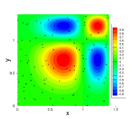
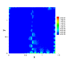
(a) (b)

Figure 3: Inverse Poisson problem: distributions of (a) the NLLSQ solution and (b) its point-wise absolute error, with the random measurement points shown in (a) as “+” symbols. Two uniform sub-domains (along $x$), local NN $[2,400,1]$, $Q=25\times 25$, $Q_{s}=50$, $R_{m}=2.0$, $\lambda_{mea}$=1, $\epsilon$=0 (no noise in measurement data).

Henceforth $Q$ denotes the number of uniform collocation points per sub-domain, $Q_{s}$ denotes the number of random measurement points per sub-domain, $\epsilon$ denotes the noise level, and $M$ denotes the number of trainable parameters of each local NN. $R_{m}$ denotes a constant, and the hidden-layer coefficients are assigned to uniform random values generated on $[-R_{m},R_{m}]$. The $R_{m}$ values employed in the tests are obtained by the method from DongY2022rm , as noted in Remark 2.5. After the NN is trained, it is evaluated on another set of $Q_{eval}=101\times 101$ uniform grid points (evaluation points) on each sub-domain to obtain $u$, which is compared with (53) to compute the errors. The relative errors of $\alpha$ ($e_{\alpha}$) and $u$ ($l^{\infty}$ and $l^{2}$ norms) are defined as,

$$\footnotesize e_{\alpha}=\frac{\left|\alpha-\alpha_{ex}\right|}{\left|\alpha_{ex}\right|},\ l^{\infty}\text{-u}=\frac{\max\left\{\left|u(\mathbf{x}_{i})-u_{ex}(\mathbf{x}_{i})\right|\right\}_{i=1}^{NQ_{eval}}}{\sqrt{\frac{1}{NQ_{eval}}\sum_{i=1}^{NQ_{eval}}u_{ex}^{2}(\mathbf{x}_{i})}},\ l^{2}\text{-u}=\frac{\sqrt{\frac{1}{NQ_{eval}}\sum_{i=1}^{NQ_{eval}}[u(\mathbf{x}_{i})-u_{ex}(\mathbf{x}_{i})]^{2}}}{\sqrt{\frac{1}{NQ_{eval}}\sum_{i=1}^{NQ_{eval}}u_{ex}^{2}(\mathbf{x}_{i})}},$$ (55)

where $N$ is the number of sub-domains and $\mathbf{x}_{i}$ denotes the evaluation points.

Figure 3 illustrates $u(x,y)$ and its point-wise absolute error obtained by the NLLSQ algorithm with $2$ sub-domains. The caption lists the main simulation parameters. In particular, the random measurement points ($100$ total) are shown in Figure 3(a), and the there is no noise in the measurement data. The NLLSQ solution for $u$ is quite accurate, with a maximum error on the order of $10^{-7}$ in the domain. The relative (or absolute) error of the computed $\alpha$ is $9.03\times 10^{-9}$.

$Q$	$\alpha$ (NLLSQ)	$\alpha$ (VarPro-F1)	$\alpha$ (VarPro-F2)
5$\times$5	1.076466245043E+0	9.982719409724E-1	0.000000000000E+0
10$\times$10	9.999867935849E-1	9.999965494049E-1	-3.188390321381E-5
15$\times$15	1.000000029498E+0	9.999999954822E-1	9.999999998978E-1
20$\times$20	9.999999999701E-1	9.999999999592E-1	9.999999999536E-1
25$\times$25	9.999999987249E-1	1.000000000817E+0	1.000000001279E+0
30$\times$30	1.000000002811E+0	1.000000000906E+0	1.000000000002E+0
35$\times$35	1.000000001708E+0	1.000000000670E+0	1.000000000237E+0
40$\times$40	1.000000001552E+0	1.000000000717E+0	1.000000000183E+0

Table 1: Inverse Poisson problem: computed $\alpha$ by the NLLSQ, VarPro-F1 and VarPro-F2 algorithms versus $Q$ (number of collocation points). Single sub-domain, NN $[2,600,1]$, $Q_{s}=100$, $\lambda_{mea}$=1, $\epsilon$=0; $R_{m}=3.0$ with NLLSQ, $R_{m}=2.8$ with VarPro-F1, and $R_{m}=2.0$ with VarPro-F2.

		NLLSQ			VarPro-F1			VarPro-F2
$Q$	$e_{\alpha}$	$l^{\infty}$-u	$l^{2}$-u	$e_{\alpha}$	$l^{\infty}$-u	$l^{2}$-u	$e_{\alpha}$	$l^{\infty}$-u	$l^{2}$-u
5$\times$5	7.65E-2	1.98E-1	2.59E-2	1.73E-3	5.70E-1	3.00E-2	1.00E+0	8.23E+1	6.65E+0
10$\times$10	1.32E-5	9.01E-3	7.88E-4	3.45E-6	1.14E-2	6.32E-4	1.00E+0	1.06E+3	5.08E+1
15$\times$15	2.95E-8	5.15E-5	3.50E-6	4.52E-9	3.50E-5	2.15E-6	1.02E-10	4.19E-6	2.40E-7
20$\times$20	2.99E-11	2.98E-7	1.56E-8	4.08E-11	1.93E-7	1.30E-8	4.64E-11	2.06E-7	1.05E-8
25$\times$25	1.28E-9	7.06E-8	8.17E-9	8.17E-10	4.46E-8	4.00E-9	1.28E-9	7.37E-8	5.96E-9
30$\times$30	2.81E-9	9.13E-8	7.13E-9	9.06E-10	6.75E-8	3.61E-9	2.44E-12	7.58E-8	7.14E-9
35$\times$35	1.71E-9	1.53E-7	1.16E-8	6.70E-10	1.02E-7	5.62E-9	2.37E-10	1.75E-7	1.55E-8
40$\times$40	1.55E-9	2.09E-7	1.69E-8	7.17E-10	1.64E-7	9.29E-9	1.83E-10	1.16E-7	1.19E-8

Table 2: Inverse Poisson problem: relative errors of $\alpha$ and $u$ versus $Q$ computed by the NLLSQ, VarPro-F1 and VarPro-F2 algorithms. Single sub-domain, NN $[2,600,1]$, $Q_{s}=100$, $\lambda_{mea}$=1, $\epsilon$=0; $R_{m}=3.0$ with NLLSQ, $R_{m}=2.8$ with VarPro-F1, and $R_{m}=2.0$ with VarPro-F2.

The convergence of computation results with respect to $Q$ (number of collocation points) is illustrated by Tables 1 and 2. Table 1 lists the computed $\alpha$ values versus $Q$ by the NLLSQ, VarPro-F1 and VarPro-F2 methods. Table 2 lists the relative errors of $\alpha$ and $u$ with respect to $Q$ from the three methods. The main parameters values for these tests are provided in the table captions. The $\alpha$ and the $u$ errors generally decrease exponentially with increasing $Q$, until $Q$ reaches a certain level. The errors generally stagnate as $Q$ further increases beyond that point.

		NLLSQ			VarPro-F1			VarPro-F2
$M$	$e_{\alpha}$	$l^{\infty}$-u	$l^{2}$-u	$e_{\alpha}$	$l^{\infty}$-u	$l^{2}$-u	$e_{\alpha}$	$l^{\infty}$-u	$l^{2}$-u
100	1.05E+4	2.87E+0	1.02E+0	1.61E+6	2.46E+0	9.98E-1	5.66E-1	2.20E+0	5.08E-1
200	1.41E-2	1.99E-1	3.23E-2	3.19E-4	1.35E-1	1.89E-2	3.91E-4	3.27E-2	4.90E-3
300	2.77E-5	2.83E-3	4.00E-4	8.68E-6	1.74E-3	1.96E-4	6.93E-7	3.27E-4	2.39E-5
400	2.82E-7	5.68E-5	4.36E-6	6.97E-9	2.37E-5	2.09E-6	9.53E-9	3.39E-6	2.21E-7
500	1.20E-8	1.81E-6	1.68E-7	5.68E-8	7.28E-7	1.07E-7	1.00E-8	4.03E-7	2.26E-8
600	1.28E-9	7.06E-8	8.17E-9	8.17E-10	4.46E-8	4.00E-9	1.28E-9	7.37E-8	5.96E-9

Table 3: Inverse Poisson problem: $\alpha$ and $u$ relative errors versus $M$ (number of training parameters) obtained by the NLLSQ, VarPro-F1 and VarPro-F2 algorithms. Single sub-domain, NN $[2,M,1]$, $Q=25\times 25$, $Q_{s}=100$, $\lambda_{mea}$=1, $\epsilon$=0; $R_{m}=3.0$ with NLLSQ, $R_{m}=2.8$ with VarPro-F1, and $R_{m}=2.0$ with VarPro-F2.

The convergence of the NLLSQ, VarPro-F1 and VarPro-F2 algorithms with respect to the number of trainable parameters $M$ is illustrated by Table 3. A single sub-domain and a single hidden layer in the neural network are employed in the simulations, where the number of hidden nodes ($M$) is varied. The caption lists the crucial parameter values. It is evident that the errors for $\alpha$ and $u$ decrease exponentially with increasing number of training parameters.

		NLLSQ			VarPro-F1			VarPro-F2
$Q_{s}$	$e_{\alpha}$	$l^{\infty}$-u	$l^{2}$-u	$e_{\alpha}$	$l^{\infty}$-u	$l^{2}$-u	$e_{\alpha}$	$l^{\infty}$-u	$l^{2}$-u
1	1.02E+0	1.01E+0	3.27E-1	1.63E+0	2.09E+1	7.27E+0	6.61E-4	1.19E-3	3.59E-4
2	5.01E-7	3.67E-6	3.80E-7	1.70E+0	3.10E+1	1.15E+1	1.67E-8	5.60E-7	3.49E-8
3	5.06E-8	3.67E-6	2.64E-7	9.64E-8	9.11E-7	9.59E-8	4.17E-9	5.46E-7	3.26E-8
5	3.06E-8	3.67E-6	2.62E-7	2.81E-8	8.88E-7	8.26E-8	7.30E-9	5.33E-7	3.25E-8
10	1.39E-8	3.67E-6	2.61E-7	1.34E-8	9.05E-7	8.12E-8	4.72E-8	5.39E-7	4.16E-8
20	5.14E-8	3.67E-6	2.63E-7	1.19E-8	9.04E-7	8.10E-8	2.62E-9	5.47E-7	3.46E-8
50	1.07E-8	3.67E-6	2.62E-7	6.63E-9	8.56E-7	8.02E-8	4.81E-10	5.33E-7	3.23E-8
100	3.26E-8	3.72E-6	2.62E-7	3.15E-9	9.29E-7	7.95E-8	1.17E-8	5.48E-7	3.27E-8

Table 4: Inverse Poisson problem: $\alpha$ and $u$ relative errors versus $Q_{s}$ (number of measurement points) for the NLLSQ, VarPro-F1 and VarPro-F2 algorithms. Single sub-domain, neural network $[2,500,1]$, $Q=30\times 30$; $R_{m}=3.0$ with NLLSQ, $R_{m}=2.8$ with VarPro-F1, and $R_{m}=2.0$ with VarPro-F2; $\lambda_{mea}$=1, $\epsilon$=0.

Table 4 illustrates the effect of the number of random measurement points ($Q_{s}$) on the $\alpha$ and $u$ errors computed by the NLLSQ, VarPro-F1 and VarProf-F2 algorithms. When $Q_{s}$ is very small, the computed $\alpha$ and $u$ are inaccurate or less accurate. On the other hand, when $Q_{s}$ reaches a certain value ($Q_{s}=3$ for this problem) and beyond, the three algorithms produce highly accurate results. This seems to be a common characteristic of these algorithms for all the test problems considered in this work.

$\epsilon$	computed-$\alpha$	$\epsilon$	computed-$\alpha$	$\epsilon$	computed-$\alpha$
0.0	9.99999993208E-1	0.01	9.9875752E-1	0.1	9.8779390E-1
0.001	9.9987537E-1	0.03	9.9630066E-1	0.2	9.7602056E-1
0.002	9.9975066E-1	0.05	9.9383633E-1	0.5	9.4329282E-1
0.005	9.9937764E-1	0.07	9.9139103E-1	0.7	9.2316247E-1
0.007	9.9912874E-1	0.09	9.8897497E-1	1.0	8.9557261E-1

Table 5: Inverse Poisson problem: $\alpha$ obtained by the NLLSQ algorithm corresponding to several noise levels ($\epsilon$). Single sub-domain, NN $[2,500,1]$, $Q=25\times 25$, $Q_{s}=50$, $R_{m}=3.0$, $\lambda_{mea}$=1.

		NLLSQ			VarPro-F1			VarPro-F2
$\epsilon$	$e_{\alpha}$	$l^{\infty}$-u	$l^{2}$-u	$e_{\alpha}$	$l^{\infty}$-u	$l^{2}$-u	$e_{\alpha}$	$l^{\infty}$-u	$l^{2}$-u
0.0	6.79E-9	1.81E-6	1.93E-7	5.93E-8	7.59E-7	1.38E-7	4.20E-10	4.50E-7	2.31E-8
0.001	1.25E-4	2.79E-4	8.04E-5	1.33E-4	2.82E-4	8.50E-5	1.23E-4	2.81E-4	7.85E-5
0.005	6.22E-4	1.39E-3	4.01E-4	6.73E-4	1.42E-3	4.29E-4	6.10E-4	1.41E-3	3.92E-4
0.01	1.24E-3	2.79E-3	8.02E-4	1.35E-3	2.85E-3	8.61E-4	1.22E-3	2.81E-3	7.82E-4
0.05	6.16E-3	1.39E-2	4.00E-3	6.63E-3	1.42E-2	4.26E-3	6.49E-3	1.41E-2	4.07E-3
0.1	1.22E-2	2.79E-2	7.98E-3	1.33E-2	2.86E-2	8.58E-3	1.19E-2	2.81E-2	7.75E-3
0.5	5.67E-2	1.42E-1	3.90E-2	6.08E-2	1.44E-1	4.17E-2	5.52E-2	1.43E-1	3.78E-2
1.0	1.04E-1	2.88E-1	7.63E-2	1.11E-1	2.93E-1	8.14E-2	1.08E-1	2.90E-1	7.62E-2

Table 6: Inverse Poisson problem: $\alpha$ and $u$ relative errors versus $\epsilon$ (noise level) computed by the NLLSQ, VarPro-F1 and VarPro-F2 algorithms. Single sub-domain, NN $[2,500,1]$, $Q=25\times 25$, $Q_{s}=50$, $\lambda_{mea}$=1; $R_{m}=3.0$ with NLLSQ, $R_{m}=2.8$ with VarPro-F1, and $R_{m}=2.0$ with VarPro-F2.

		$\lambda_{mea}$=0.5			$\lambda_{mea}$=0.25			$\lambda_{mea}$=0.1
$\epsilon$	$e_{\alpha}$	$l^{\infty}$-u	$l^{2}$-u	$e_{\alpha}$	$l^{\infty}$-u	$l^{2}$-u	$e_{\alpha}$	$l^{\infty}$-u	$l^{2}$-u
0.0	1.69E-8	1.81E-6	2.27E-7	2.25E-8	1.82E-6	2.46E-7	1.34E-8	1.81E-6	2.49E-7
0.001	1.04E-4	1.80E-4	5.58E-5	9.79E-5	1.75E-4	5.23E-5	9.58E-5	1.73E-4	5.19E-5
0.005	5.22E-4	9.01E-4	2.79E-4	4.89E-4	8.72E-4	2.61E-4	4.79E-4	8.61E-4	2.59E-4
0.01	1.04E-3	1.80E-3	5.58E-4	9.76E-4	1.74E-3	5.22E-4	9.56E-4	1.72E-3	5.18E-4
0.05	5.16E-3	8.94E-3	2.77E-3	4.83E-3	8.65E-3	2.59E-3	4.73E-3	8.54E-3	2.57E-3
0.1	1.02E-2	1.78E-2	5.49E-3	9.54E-3	1.71E-2	5.13E-3	9.33E-3	1.69E-2	5.08E-3
0.5	4.66E-2	8.35E-2	2.59E-2	4.33E-2	8.00E-2	2.39E-2	4.23E-2	7.88E-2	2.36E-2
1.0	8.45E-2	1.56E-1	4.83E-2	7.78E-2	1.48E-1	4.40E-2	7.57E-2	1.45E-1	4.33E-2

Table 7: Inverse Poisson problem: $\alpha$ and $u$ relative errors versus $\epsilon$ and $\lambda_{mea}$ (scaling coefficient of measurement residual) computed by the NLLSQ algorithm. Single sub-domain, NN $[2,500,1]$, $Q=25\times 25$, $Q_{s}=50$, $R_{m}=3.0$. These can be compared with the NLLSQ data in Table 6, which is with $\lambda_{mea}=1$.

In the foregoing tests no noise is considered in the measurement data ($\epsilon=0$). Tables 5, 6 and 7 demonstrate the effect of noisy measurement data on the computation results. Table 5 shows the computed $\alpha$ values by the NLLSQ algorithm corresponding to different noise levels, ranging from $\epsilon=0$ ($0\%$) to $\epsilon=1.0$ ($100\%$). Table 6 lists the $\alpha$ errors and the $u$ errors corresponding to several noise levels obtained by the NLLSQ, VarPro-F1 and VarPro-F2 algorithms. Table 7 provides the $\alpha$ and $u$ relative errors corresponding to different $\epsilon$ and several $\lambda_{mea}$ (scaling factor of measurement residual) values with the NLLSQ algorithm. The presence of noise degrades the simulation accuracy. But the current method and these algorithms appear to be quite robust. For example, with $10\%$ ($\epsilon=0.1$) noise in the measurement data the relative error of $\alpha$ is around $1\%$ for the three methods. With $100\%$ ($\epsilon=1.0$) noise in the data, the computed $\alpha$ exhibits a relative error around $10\%$ with these algorithms. For noisy data, scaling the measurement residual by $\lambda_{mea}$ can improve the accuracy of computation results and make the method more robust (see Table 7), compared with the case of no scaling. A smaller $\lambda_{mea}$ in general leads to a better accuracy.

3.2 Parametric Advection Equation

Consider the spatial-temporal domain, $(x,t)\in\Omega=[0,3]\times[0,1]$, and the following inverse problem,

$$\frac{\partial u}{\partial t}-c\frac{\partial u}{\partial x}=0,$$ (56a)

$$u(0,t)=u(3,t),\quad u(x,0)=10\sinh\left[\frac{1}{10}\sin\frac{2\pi}{3}\left(x-\frac{5}{2}\right)\right],$$ (56b)

$$u(\xi_{i},\eta_{i})=S(\xi_{i},\eta_{i}),\quad(\xi_{i},\eta_{i})\in\mathbb{Y}\subset\Omega,\ 1\leqslant i\leqslant NQ_{s},$$ (56c)

where $\mathbb{Y}$ denotes the set of measurement points in $\Omega$. The wave speed $c$ and the field $u(x,t)$ are the unknowns to be determined in this problem. We employ the following exact solution to this problem in the tests,

$$\small\begin{split}&c_{ex}=3,\quad u_{ex}(x,t)=10\sinh\left[\frac{1}{10}\sin\frac{2\pi}{3}\left(x+3t-\frac{5}{2}\right)\right].\end{split}$$ (57)

We employ random measurement points in $\Omega$, and the measurement data are given by (54), in which $u_{ex}$ is given by (57). The notations adopted below (e.g. $Q$, $M$, $N$, $Q_{s}$, $R_{m}$, $\epsilon$) are the same as in Section 3.1. The $l^{\infty}$ and $l^{2}$ norms of the $u$ relative error reported below are computed on a set of $Q_{eval}=101\times 101$ uniform grid points in each sub-domain after the network is trained.

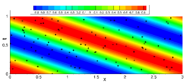
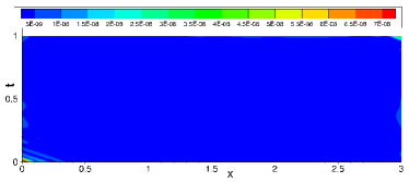
(a) (b)

Figure 4: Inverse advection problem: distributions of (a) the NLLSQ solution for $u(x,t)$ and (b) its point-wise absolute error, with the random measurement points shown in (a) as “+” symbols. Single sub-domain, NN $[2,400,1]$, $Q=25\times 25$ (collocation points), $Q_{s}=100$ (measurement points), $R_{m}=2.5$, $\lambda_{mea}$=1, $\epsilon=0$ (no noise in measurement).

Figure 4 illustrates the distributions of the NLLSQ solution for $u(x,t)$ and its point-wise absolute error in $\Omega$. The crucial simulation parameters are listed in the figure caption. The solution is highly accurate, with a maximum error on the level $10^{-8}$ in the domain. The computed wave speed $c$ has a relative error $2.82\times 10^{-10}$ for this case.

$Q$	$c$ (NLLSQ)	$c$ (VarPro-F1)	$c$ (VarPro-F2)
5$\times$5	3.000074167561E+0	2.999935510214E+0	6.785575335360E-1
10$\times$10	2.999998340831E+0	3.000000635012E+0	6.785578125741E-1
15$\times$15	2.999999999982E+0	2.999999999967E+0	-7.284017530389E-2
20$\times$20	3.000000000029E+0	3.000000000041E+0	3.000000000378E+0
25$\times$25	3.000000000845E+0	3.000000000869E+0	3.000000000025E+0
30$\times$30	3.000000000534E+0	3.000000000542E+0	3.000000001047E+0
35$\times$35	3.000000000596E+0	3.000000000596E+0	3.000000001295E+0
40$\times$40	3.000000000771E+0	3.000000000770E+0	3.000000001534E+0

Table 8: Inverse advection problem: the computed $c$ versus $Q$ obtained by the NLLSQ, VarPro-F1 and VarPro-F2 algorithms. Single sub-domain, NN $[2,400,1]$, $Q_{s}=100$; $R_{m}=2.5$ with NLLSQ and VarPro-F1, and $R_{m}=2.0$ with VarPro-F2; $\lambda_{mea}$=1, $\epsilon=0$.

		NLLSQ			VarPro-F1			VarPro-F2
$Q$	$e_{c}$	$l^{\infty}$-u	$l^{2}$-u	$e_{c}$	$l^{\infty}$-u	$l^{2}$-u	$e_{c}$	$l^{\infty}$-u	$l^{2}$-u
5$\times$5	2.47E-5	4.56E-2	4.60E-3	2.15E-5	2.03E-2	2.19E-3	7.74E-1	1.51E+2	1.46E+1
10$\times$10	5.53E-7	5.25E-4	5.70E-5	2.12E-7	3.16E-4	2.56E-5	7.74E-1	1.66E+3	1.11E+2
15$\times$15	5.91E-12	8.55E-6	3.50E-7	1.12E-11	8.76E-6	3.57E-7	1.02E+0	1.83E+4	5.68E+2
20$\times$20	9.74E-12	2.28E-7	8.31E-9	1.37E-11	2.31E-7	8.14E-9	1.26E-10	4.38E-7	1.42E-8
25$\times$25	2.82E-10	1.08E-7	3.50E-9	2.90E-10	1.09E-7	3.49E-9	8.47E-12	1.67E-7	5.47E-9
30$\times$30	1.78E-10	8.29E-8	3.23E-9	1.81E-10	8.29E-8	3.24E-9	3.49E-10	9.89E-8	5.13E-9
35$\times$35	1.99E-10	7.30E-8	3.95E-9	1.99E-10	7.29E-8	3.95E-9	4.32E-10	6.27E-8	5.39E-9
40$\times$40	2.57E-10	6.58E-8	4.67E-9	2.57E-10	6.57E-8	4.67E-9	5.11E-10	4.87E-8	5.77E-9

Table 9: Inverse advection problem: $c$ and $u$ relative errors versus $Q$ obtained by the NLLSQ, VarPro-F1 and VarPro-F2 algorithms. Single sub-domain, NN $[2,400,1]$, $Q_{s}=100$, $\lambda_{mea}$=1, $\epsilon$=0; $R_{m}=2.5$ with NLLSQ and VarPro-F1, and $R_{m}=2.0$ with VarPro-F2. $e_{c}$ denotes the relative error of $c$.

		NLLSQ			VarPro-F1			VarPro-F2
$M$	$e_{c}$	$l^{\infty}$-u	$l^{2}$-u	$e_{c}$	$l^{\infty}$-u	$l^{2}$-u	$e_{c}$	$l^{\infty}$-u	$l^{2}$-u
50	1.97E-2	1.69E-1	5.53E-2	1.97E-2	1.69E-1	5.53E-2	5.56E-3	9.33E-2	2.66E-2
100	8.79E-4	3.71E-2	2.18E-2	8.79E-4	3.71E-2	2.18E-2	8.57E-6	4.25E-3	1.60E-3
200	1.66E-6	1.10E-4	2.03E-5	1.66E-6	1.10E-4	2.03E-5	1.80E-6	8.04E-5	2.12E-5
300	9.84E-9	4.12E-6	4.96E-7	9.84E-9	4.12E-6	4.96E-7	6.65E-9	1.21E-6	8.44E-8
400	8.05E-11	1.11E-7	3.96E-9	6.54E-11	1.11E-7	3.98E-9	5.02E-10	1.62E-7	6.07E-9

Table 10: Inverse advection problem: $c$ and $u$ relative errors versus $M$ (number of training parameters) obtained with the NLLSQ, VarPro-F1 and VarPro-F2 algorithms. Single sub-domain, NN $[2,M,1]$, $Q=25\times 25$, $Q_{s}=50$, $\lambda_{mea}$=1, $\epsilon$=0; $R_{m}=2.5$ with NLLSQ and VarPro-F1, and $R_{m}=2.0$ with VarPro-F2.

The convergence behaviors of the computed $c$ and $u$ with respect to the collocation points ($Q$) and to the training parameters ($M$) are illustrated in Tables 8 to 10 (without noise). Table 8 and Table 9 list the computed $c$ values, and the relative errors of $c$ errors and $u$, for several sets of uniform collocation points obtained by the NLLSQ, VarPro-F1 and VarPro-F2 algorithms. Table 10 shows the $c$ errors and the $u$ errors for several sets of training parameters with the three algorithms. One can observe the general exponential convergence of the $c$ and $u$ errors with respect to $Q$ and to $M$. Tables 8 and 9 indicate that the convergence of VarPro-F2 with respect to $Q$ is not quite regular. If the set of collocation points is too small ($Q=15\times 15$ and below), the computed VarPro-F2 results are not accurate.

$\epsilon$	computed $c$	$\epsilon$	computed $c$	$\epsilon$	computed $c$
0.0	3.000000000534E+0	0.01	2.9997368E+0	0.1	2.9971795E+0
0.001	2.9999739E+0	0.03	2.9991975E+0	0.2	2.9937846E+0
0.002	2.9999477E+0	0.05	2.9986396E+0	0.5	2.9779459E+0
0.005	2.9998688E+0	0.07	2.9980677E+0	0.7	2.9570522E+0
0.007	2.9998158E+0	0.09	2.9974839E+0	1.0	2.8441808E+0

Table 11: Inverse advection problem: $c$ computed by the NLLSQ algorithm corresponding to several noise levels $\epsilon$. Single sub-domain, NN $[2,400,1]$, $Q=30\times 30$, $Q_{s}=100$, $R_{m}=2.5$, $\lambda_{mea}$=1.

		NLLSQ			VarPro-F1			VarPro-F2
$\epsilon$	$e_{c}$	$l^{\infty}$-u	$l^{2}$-u	$e_{c}$	$l^{\infty}$-u	$l^{2}$-u	$e_{c}$	$l^{\infty}$-u	$l^{2}$-u
0.0	1.78E-10	8.29E-8	3.23E-9	1.81E-10	8.29E-8	3.24E-9	3.49E-10	9.89E-8	5.13E-9
0.001	8.72E-6	4.91E-4	1.77E-4	8.73E-6	4.91E-4	1.77E-4	4.67E-6	6.91E-4	1.76E-4
0.005	4.37E-5	2.46E-3	8.85E-4	4.41E-5	2.46E-3	8.84E-4	2.26E-5	3.49E-3	8.80E-4
0.01	8.77E-5	4.91E-3	1.77E-3	8.81E-5	4.91E-3	1.77E-3	4.61E-5	7.00E-3	1.76E-3
0.05	4.53E-4	2.46E-2	8.84E-3	4.55E-4	2.45E-2	8.84E-3	2.49E-4	3.50E-2	8.79E-3
0.1	9.40E-4	4.92E-2	1.77E-2	9.54E-4	4.92E-2	1.77E-2	5.53E-4	6.95E-2	1.76E-2
0.5	7.35E-3	2.47E-1	8.90E-2	7.40E-3	2.47E-1	8.90E-2	5.42E-3	3.59E-1	8.86E-2
1.0	5.19E-2	5.04E-1	2.06E-1	5.19E-2	5.04E-1	2.06E-1	3.78E-2	8.03E-1	1.95E-1

Table 12: Inverse advection problem: $c$ and $u$ relative errors versus $\epsilon$ obtained with the NLLSQ, VarPro-F1 and VarPro-F2 algorithms. Single sub-domain, NN $[2,400,1]$, $Q=30\times 30$, $Q_{s}=100$, $\lambda_{mea}$=1; $R_{m}=2.5$ with NLLSQ and VarPro-F1, and $R_{m}=2.0$ with VarPro-F2.

		$\lambda_{mea}$=0.25			$\lambda_{mea}$=0.1
$\epsilon$	$e_{c}$	$l^{\infty}$-u	$l^{2}$-u	$e_{c}$	$l^{\infty}$-u	$l^{2}$-u
0.0	2.31E-10	8.53E-8	4.31E-9	2.32E-10	8.51E-8	4.66E-9
0.001	2.71E-6	6.68E-5	3.19E-5	2.60E-6	2.84E-5	1.10E-5
0.005	1.36E-5	3.34E-4	1.59E-4	1.30E-5	1.42E-4	5.49E-5
0.01	2.71E-5	6.68E-4	3.19E-4	2.61E-5	2.85E-4	1.10E-4
0.05	1.37E-4	3.34E-3	1.59E-3	1.31E-4	1.43E-3	5.52E-4
0.1	2.75E-4	6.69E-3	3.19E-3	2.65E-4	2.88E-3	1.11E-3
0.5	1.46E-3	3.35E-2	1.60E-2	1.44E-3	1.54E-2	5.89E-3
1.0	3.25E-3	6.74E-2	3.21E-2	3.25E-3	3.38E-2	1.29E-2

Table 13: Inverse advection problem: $c$ and $u$ relative errors versus $\epsilon$ and $\lambda_{mea}$ (scaling coefficient of measurement residual) obtained with the NLLSQ algorithm. Single sub-domain, NN $[2,400,1]$, $Q=30\times 30$, $Q_{s}=100$, $R_{m}=2.5$. These can be compared with the NLLSQ data in Table 12 for $\lambda_{mea}$=1.

The effects of noisy measurement data on the computation accuracy are illustrated by Tables 11 through 13. Table 11 lists the computed $c$ by the NLLSQ algorithm corresponding to several noise levels $\epsilon$ in the measurement data. Table 12 shows the $c$ and $u$ relative errors corresponding to different noise levels, computed by the NLLSQ, VarPro-F1 and VarPro-F2 algorithms. Table 13 shows the relative errors for $c$ and $u$ corresponding to different noise levels and several $\lambda_{mea}$ values, illustrating the effect of scaling the measurement residual (see Remark 2.6). The computation results are observed to be quite robust to the noise in the measurement. For example, with $10\%$ noise ($\epsilon=0.1$) in the measurement, the relative errors of $c$ computed by these methods are generally on the level of $0.1\%$ (see Table 12). Scaling the measurement residual by $\lambda_{mea}<1$ can markedly improve the simulation accuracy in the presence of noise, but slightly degrades the accuracy for the noise-free data; see Table 13.

3.3 Parametric Nonlinear Helmholtz Equation

Consider the 2D domain, $(x,y)\in\Omega=[0,1.4]\times[0,1.4]$, and the inverse problem on $\Omega$,

$$\frac{\partial^{2}u}{\partial x^{2}}+\frac{\partial^{2}u}{\partial y^{2}}-\alpha_{1}u+\alpha_{2}\cos(2u)=f(x,y),$$ (58a)

$$u(0,y)=g_{1}(y),\quad u(1.4,y)=g_{2}(y),\quad u(x,0)=g_{3}(x),\quad u(x,1.4)=g_{4}(x),$$ (58b)

$$u(\xi_{i},\eta_{i})=S(\xi_{i},\eta_{i}),\quad(\xi_{i},\eta_{i})\in\mathbb{Y}\subset\Omega,\ 1\leqslant i\leqslant NQ_{s},$$ (58c)

where $f$ and $g_{i}$ ($1\leqslant i\leqslant 4$) are prescribed source term and boundary data, $\mathbb{Y}$ denotes the set of random measurement points in $\Omega$, and the parameters $(\alpha_{1},\alpha_{2})$ and the field $u(x,y)$ are the unknowns to be determined. We consider the following manufactured solution to this problem in the tests,

$$\small\begin{split}&\alpha_{1}^{ex}=100,\quad\alpha_{2}^{ex}=5,\quad u_{ex}(x,y)=\cos(\pi x^{2})\cos(\pi y^{2}).\end{split}$$ (59)

The measurement data $S(\xi_{i},\eta_{i})$ ($1\leqslant i\leqslant NQ_{s}$) are given by (54), in which $u_{ex}$ is given by (59). The $u$ errors are computed on a set of $101\times 101$ uniform grid points in each sub-domain after the neural network is trained. The notations below follow those of the previous sub-sections.

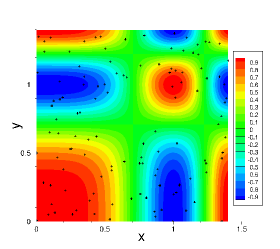
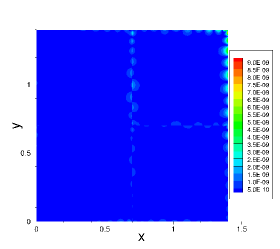
(a) (b)

Figure 5: Inverse nonlinear Helmholtz problem: distributions of (a) the VarPro-F1 solution for $u(x,y)$ and (b) its point-wise absolute error, with the random measurement points shown in (a) as “+” symbols. Four uniform sub-domains ($2$ in each direction), local NN $[2,300,1]$, $Q=20\times 20$, $Q_{s}=30$, $R_{m}=1.5$, $\lambda_{mea}$=1, $\epsilon$=0 (no noise in measurement data).

Figure 5 shows distributions of the $u(x,y)$ solution and its point-wise absolute error computed by the VarPro-F1 algorithm on $4$ uniform sub-domains, with the $120$ random measurement points in total ($Q_{s}=30$ points per sub-domain) displayed in Figure 5(a). The figure caption lists the crucial simulation parameters for this test. VarPro-F1 exhibits a high accuracy, with the maximum $u$ error on the order of $10^{-8}$. The relative errors of the computed $\alpha_{1}$ and $\alpha_{2}$ are $3.52\times 10^{-11}$ and $4.76\times 10^{-10}$, respectively, in this test.

$Q$	computed $\alpha_{1}$	computed $\alpha_{2}$
5$\times$5	9.946591149073E+1	5.169760481373E+0
10$\times$10	9.999987125506E+1	4.999987933629E+0
15$\times$15	9.999999986638E+1	5.000000027512E+0
20$\times$20	9.999999982078E+1	4.999999813483E+0
25$\times$25	1.000000001774E+2	4.999999946859E+0
30$\times$30	1.000000001832E+2	4.999999843159E+0
35$\times$35	9.999999989070E+1	5.000000059829E+0
40$\times$40	9.999999957958E+1	5.000001280912E+0

Table 14: Inverse nonlinear Helmholtz problem: $\alpha_{1}$ and $\alpha_{2}$ versus $Q$ (number of collocation points) obtained by the NLLSQ algorithm. Single sub-domain, NN $[2,500,1]$, $Q_{s}=100$, $R_{m}=2.25$, $\epsilon=0$, $\lambda_{mea}$=1.

		NLLSQ			VarPro-F1			VarPro-F2
$Q$	$e_{\alpha_{1}}$	$e_{\alpha_{2}}$	$l^{2}$-u	$e_{\alpha_{1}}$	$e_{\alpha_{2}}$	$l^{2}$-u	$e_{\alpha_{1}}$	$e_{\alpha_{2}}$	$l^{2}$-u
5$\times$5	5.34E-3	3.40E-2	2.26E-2	2.35E-4	5.72E-4	4.16E-3	1.00E+0	1.00E+0	1.56E+0
10$\times$10	1.29E-6	2.41E-6	2.21E-4	1.29E-6	2.42E-6	2.20E-4	1.00E+0	1.00E+0	1.66E+1
15$\times$15	1.34E-9	5.50E-9	6.55E-7	8.81E-11	1.60E-9	5.64E-7	5.41E-1	3.72E-1	4.84E+1
20$\times$20	1.79E-9	3.73E-8	4.93E-8	7.48E-10	5.74E-8	5.67E-8	1.28E-8	4.63E-8	1.65E-7
25$\times$25	1.77E-9	1.06E-8	8.52E-9	1.11E-9	3.30E-9	7.12E-9	1.43E-8	2.85E-7	4.30E-8
30$\times$30	1.83E-9	3.14E-8	1.00E-8	5.46E-10	4.46E-9	8.39E-9	5.45E-9	2.24E-7	6.02E-8
35$\times$35	1.09E-9	1.20E-8	9.42E-9	2.58E-9	1.79E-7	1.18E-8	1.23E-8	3.86E-7	7.50E-8
40$\times$40	4.20E-9	2.56E-7	1.54E-8	5.14E-9	2.73E-7	1.58E-8	1.22E-8	1.85E-7	9.12E-8

Table 15: Inverse nonlinear Helmholtz problem: relative errors of $\alpha_{1}$, $\alpha_{2}$ and $u$ versus $Q$ obtained by the NLLSQ, VarPro-F1 and VarPro-F2 algorithms. Single sub-domain, NN $[2,500,1]$, $Q_{s}=100$; $R_{m}=2.25$ with NLLSQ and VarPro-F1, and $R_{m}=2.5$ with VarPro-F2; $\lambda_{mea}$=1, $\epsilon$=0. $e_{\alpha_{1}}$ and $e_{\alpha_{2}}$ denote the relative errors of $\alpha_{1}$ and $\alpha_{2}$.

The convergence of the simulation results with respect to the number of collocation points ($Q$) is illustrated by the Tables 14 and 15. Table 14 lists the computed $\alpha_{1}$ and $\alpha_{2}$ by the NLLSQ algorithm corresponding to a range of $Q$ values. Table 15 shows the relative $\alpha_{1}$ and $\alpha_{2}$ errors and the $l^{2}$ norm of the relative $u$ error corresponding to different $Q$ obtained by the NLLSQ, VarPro-F1 and VarPro-F2 algorithms. The crucial simulation parameter values are provided in the table captions. A general exponential convergence in the errors with respect to $Q$ can be observed. One can also observe that the convergence of the VarPro-F2 algorithm appears to be less regular. The VarPro-F2 results are inaccurate with a small $Q$ ($Q=15\times 15$ or less), and its errors abruptly drop to $10^{-7}\sim 10^{-8}$ as the collocation points reach $Q=20\times 20$ and beyond.

		NLLSQ			VarPro-F1			VarPro-F2
$M$	$e_{\alpha_{1}}$	$e_{\alpha_{2}}$	$l^{2}$-u	$e_{\alpha_{1}}$	$e_{\alpha_{2}}$	$l^{2}$-u	$e_{\alpha_{1}}$	$e_{\alpha_{2}}$	$l^{2}$-u
100	5.58E-1	7.37E-1	3.21E-1	5.58E-1	7.37E-1	3.21E-1	1.08E+1	3.61E+0	8.80E-1
200	4.39E-3	2.60E-3	7.66E-3	4.39E-3	2.60E-3	7.66E-3	3.70E-3	4.05E-2	1.04E-2
300	6.52E-5	7.27E-5	5.15E-5	6.51E-5	7.07E-5	5.14E-5	5.28E-5	2.58E-4	8.91E-5
400	1.08E-7	2.17E-6	6.22E-7	1.06E-7	1.80E-6	6.33E-7	3.62E-7	1.18E-5	1.12E-6
500	1.83E-9	3.14E-8	1.00E-8	5.46E-10	4.46E-9	8.39E-9	5.45E-9	2.24E-7	6.02E-8
600	5.16E-10	1.47E-8	2.14E-9	1.45E-10	5.33E-10	2.29E-9	4.47E-10	3.30E-9	1.77E-8

Table 16: Inverse nonlinear Helmholtz problem: relative errors of $\alpha_{1}$, $\alpha_{2}$ and $u$ versus $M$ (number of training parameters) obtained by the NLLSQ, VarPro-F1 and VarPro-F2 algorithms. Single sub-domain, NN $[2,M,1]$, $Q_{s}=100$, $Q=30\times 30$; $R_{m}=2.25$ with NLLSQ and VarPro-F1, and $R_{m}=2.5$ with VarPro-F2; $\epsilon$=0, $\lambda_{mea}$=1.

Table 16 illustrates the convergence of the $\alpha_{1}$, $\alpha_{2}$ and $u$ errors, obtained by the NLLSQ, VarPro-F1 and VarPro-F2 algorithms, with respect to the training parameters ($M$). The table caption lists values of the main simulation parameters. The relative errors of $\alpha_{1}$, $\alpha_{2}$ and $u$ decrease exponentially with increasing $M$.

$Q_{s}$	$\alpha_{1}$	$\alpha_{2}$	$e_{\alpha_{1}}$	$e_{\alpha_{2}}$	$l^{\infty}$-u	$l^{2}$-u
5	1.000000005409E+2	4.999994839886E+0	5.41E-9	1.03E-6	7.79E-8	4.13E-8
10	9.999999992698E+1	4.999999378668E+0	7.30E-10	1.24E-7	6.03E-8	8.65E-9
20	1.000000001181E+2	5.000000028574E+0	1.18E-9	5.71E-9	9.67E-8	8.94E-9
30	9.999999993263E+1	5.000000391330E+0	6.74E-10	7.83E-8	7.97E-8	8.18E-9
50	9.999999980057E+1	5.000000659553E+0	1.99E-9	1.32E-7	7.56E-8	1.05E-8
100	1.000000001832E+2	4.999999843159E+0	1.83E-9	3.14E-8	9.37E-8	1.00E-8

Table 17: Inverse nonlinear Helmholtz problem: the values/relative-errors of $\alpha_{1}$ and $\alpha_{2}$, and the $u$ relative errors, versus the number of random measurement points ($Q_{s}$), computed by the NLLSQ algorithm. Single sub-domain, NN $[2,500,1]$, $Q=30\times 30$, $R_{m}=2.25$, $\lambda_{mea}$=1, $\epsilon$=0.

Table 17 shows the computed $\alpha_{1}$ and $\alpha_{2}$ values, their relative errors, and the $u$ relative errors ($l^{\infty}$ and $l^{2}$ norms) obtained by the NLLSQ algorithm corresponding to a range of $Q_{s}$ (number of random measurement points). The effect of $Q_{s}$ on the errors appears to be not significant, unless $Q_{s}$ is very small. This is similar to what has been observed with linear forward PDEs (see e.g. Section 3.1).

		NLLSQ			VarPro-F1			VarPro-F2
$\epsilon$	$e_{\alpha_{1}}$	$e_{\alpha_{2}}$	$l^{2}$-u	$e_{\alpha_{1}}$	$e_{\alpha_{2}}$	$l^{2}$-u	$e_{\alpha_{1}}$	$e_{\alpha_{2}}$	$l^{2}$-u
0.0	1.99E-9	1.32E-7	1.05E-8	1.96E-11	1.76E-8	7.85E-9	7.18E-9	4.77E-7	5.95E-8
0.001	4.31E-4	1.12E-4	2.46E-4	4.31E-4	1.04E-4	2.46E-4	4.31E-4	1.45E-4	2.46E-4
0.002	8.62E-4	2.19E-4	4.92E-4	8.62E-4	2.40E-4	4.92E-4	8.62E-4	2.60E-4	4.92E-4
0.005	2.16E-3	5.21E-4	1.23E-3	2.16E-3	5.67E-4	1.23E-3	2.16E-3	6.00E-4	1.23E-3
0.01	4.32E-3	9.64E-4	2.46E-3	4.32E-3	9.54E-4	2.46E-3	4.32E-3	1.26E-3	2.46E-3
0.02	8.67E-3	1.41E-3	4.92E-3	8.67E-3	1.61E-3	4.92E-3	8.67E-3	1.84E-3	4.92E-3
0.05	2.19E-2	3.72E-4	1.23E-2	2.19E-2	6.72E-4	1.23E-2	2.19E-2	2.29E-3	1.23E-2
0.1	4.44E-2	8.72E-3	2.45E-2	4.44E-2	8.77E-3	2.45E-2	4.44E-2	7.37E-3	2.45E-2

Table 18: Inverse nonlinear Helmholtz problem: relative errors of $\alpha_{1}$, $\alpha_{2}$ and $u$ versus the noise level ($\epsilon$) in the measurement data, obtained by the NLLSQ, VarPro-F1 and VarPro-F2 algorithms. Single sub-domain, NN $[2,500,1]$, $Q=30\times 30$, $Q_{s}=50$, $\lambda_{mea}$=1; $R_{m}=2.25$ with NLLSQ and VarPro-F1, and $R_{m}=2.5$ with VarPro-F2.

		$\lambda_{mea}$=1	(no	scaling)		$\lambda_{mea}$=0.01
$\epsilon$	$e_{\alpha_{1}}$	$e_{\alpha_{2}}$	$l^{\infty}$-u	$l^{2}$-u	$e_{\alpha_{1}}$	$e_{\alpha_{2}}$	$l^{\infty}$-u	$l^{2}$-u
0.0	1.83E-7	1.57E-7	5.50E-8	5.89E-9	2.27E-4	2.87E-5	1.66E-6	7.53E-7
0.001	4.08E-2	1.28E-3	3.40E-4	1.43E-4	1.62E-2	1.36E-3	1.17E-4	5.31E-5
0.005	2.04E-1	6.46E-3	1.70E-3	7.13E-4	7.36E-2	6.07E-3	5.33E-4	2.41E-4
0.01	4.09E-1	1.30E-2	3.40E-3	1.43E-3	1.59E-1	1.32E-2	1.15E-3	5.21E-4
0.05	2.06E+0	7.05E-2	1.71E-2	7.12E-3	7.82E-1	6.42E-2	5.62E-3	2.55E-3
0.1	4.18E+0	1.50E-1	3.40E-2	1.42E-2	1.77E+0	1.40E-1	1.26E-2	5.73E-3

Table 19: Inverse nonlinear Helmholtz problem: absolute errors in $\alpha_{1}$, $\alpha_{2}$ and $u$ versus $\epsilon$ and $\lambda_{mea}$ (scaling coefficient of measurement residual) obtained by the NLLSQ method. Single sub-domain, neural network $[2,500,1]$, $Q=30\times 30$, $Q_{s}=100$, $R_{m}=2.25$.

No noise is considered in the measurement data in the foregoing tests. Table 18 illustrates the effect of the noise level ($\epsilon$) on the accuracy of the computed $\alpha_{1}$, $\alpha_{2}$ and $u$ by the NLLSQ, VarPro-F1 and VarPro-F2 algorithms. The main parameters for these simulations are listed in the table caption. The accuracy of these algorithms appears quite robust to the noise. For example, with $1\%$ noise ($\epsilon=0.01$) in the measurement data the relative errors for $\alpha_{1}$ and $\alpha_{2}$ obtained by the three methods are on the order of $0.1\%$, and with $10\%$ noise ($\epsilon=0.1$) in the measurement data the relative errors for $\alpha_{1}$ and $\alpha_{2}$ are on the order of $1\sim 4\%$.

3.4 Parametric Viscous Burgers Equation

Consider the spatial-temporal domain, $(x,t)\in\Omega=[0,2]\times[0,1.5]$, and the inverse problem with the parametric Burgers’ equation,

$$\frac{\partial u}{\partial t}+\alpha_{1}u\frac{\partial u}{\partial x}=\alpha_{2}\frac{\partial^{2}u}{\partial x^{2}}+f(x,t),$$ (60a)

$$u(0,t)=g_{1}(t),\quad u(2,t)=g_{2}(t),\quad u(x,0)=h(x),$$ (60b)

$$u(\xi_{i},\eta_{i})=S(\xi_{i},\eta_{i}),\quad(\xi_{i},\eta_{i})\in\mathbb{Y}\subset\Omega,\ 1\leqslant i\leqslant NQ_{s},$$ (60c)

where $f$ is a prescribed source term, $g_{1}$ and $g_{2}$ are prescribed Dirichlet boundary data, $h$ is the initial distribution, the constants $\alpha_{i}$ ($i=1,2$) and the field $u(x,t)$ are the unknowns to be solved for, $\mathbb{Y}$ denotes the set of random measurement points, $N$ is the number of sub-domains, and $Q_{s}$ is the number of measurement points per sub-domain. We employ the following manufactured solution in the tests,

$$\small\left\{\small\begin{split}&\alpha_{1}^{ex}=0.1,\quad\alpha_{2}^{ex}=0.01,\\ &u_{ex}(x,t)=\left(1+\frac{x}{20}\right)\left(1+\frac{t}{20}\right)\left[\frac{3}{2}\cos\left(\pi x+\frac{7\pi}{20}\right)+\frac{27}{20}\cos\left(2\pi x-\frac{3\pi}{5}\right)\right]\left[\frac{3}{2}\cos\left(\pi t+\frac{7\pi}{20}\right)\right.\\ &\qquad\qquad\ \ \left.+\frac{27}{20}\cos\left(2\pi t-\frac{3\pi}{5}\right)\right].\end{split}\right.$$ (61)

The source term $f$ and the boundary/initial data are chosen such that the expressions in (61) satisfy the equations (60a)–(60b). The measurement data $S(\xi_{i},\eta_{i})$ is assumed to be given by (54), in which $u_{ex}$ is given by (61). In the following the $u$ errors are computed on a $101\times 101$ uniform grid points in each sub-domain, and we adopt the same notations (e.g. $Q$, $Q_{s}$, $M$, $R_{m}$ and $\epsilon$) as in previous sub-sections.

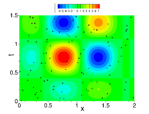
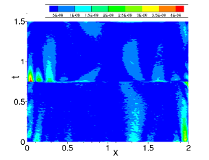
(a) (b)

Figure 6: Inverse Burgers’ problem: distributions of (a) the NLLSQ solution and (b) its point-wise absolute error, with the random measurement points shown by the “+” symbols in (a). Two uniform sub-domains (along $t$), local NN $[2,300,1]$, $Q=25\times 25$, $Q_{s}=50$, $R_{m}=1.5$, $\epsilon$=0 (no noise in measurement data), $\lambda_{mea}$=1.

Figure 6 illustrates the $u(x,t)$ solution and its point-wise absolute error computed by the NLLSQ algorithm with two uniform sub-domains along $t$, and the $100$ random measurement points ($50$ points per sub-domain) in the domain are shown in Figure 6(a). The figure caption provides the main parameter values in this simulation. The results signify a high accuracy for the computed $u$ solution, with the maximum error on the order of $10^{-8}$. The relative errors of the computed $\alpha_{1}$ and $\alpha_{2}$ are $1.30\times 10^{-9}$ and $1.48\times 10^{-8}$, respectively, for this simulation.

$Q$	$\alpha_{1}$	$\alpha_{2}$
5$\times$5	9.999660775275E-2	9.994514983290E-3
10$\times$10	9.999998874379E-2	9.999992607237E-3
15$\times$15	1.000000000074E-1	1.000000000018E-2
20$\times$20	1.000000000060E-1	1.000000000487E-2
25$\times$25	9.999999999967E-2	9.999999999698E-3
30$\times$30	1.000000000049E-1	9.999999998052E-3

Table 20: Inverse Burgers’ problem: the computed $\alpha_{1}$ and $\alpha_{2}$ versus $Q$ (number of collocation points) obtained with the NLLSQ algorithm. Single sub-domain, NN $[2,400,1]$, $Q_{s}=100$, $R_{m}=1.9$, $\lambda_{mea}$=1, $\epsilon$=0.

		NLLSQ			VarPro-F1			VarPro-F2
$Q$	$e_{\alpha_{1}}$	$e_{\alpha_{2}}$	$l^{2}$-u	$e_{\alpha_{1}}$	$e_{\alpha_{2}}$	$l^{2}$-u	$e_{\alpha_{1}}$	$e_{\alpha_{2}}$	$l^{2}$-u
5$\times$5	3.39E-5	5.49E-4	8.77E-4	3.75E-5	5.96E-4	8.64E-4	3.04E-1	5.71E-1	6.24E+0
10$\times$10	1.13E-7	7.39E-7	8.89E-6	1.09E-7	6.84E-7	8.57E-6	9.79E-1	1.66E+1	7.06E+1
15$\times$15	7.40E-11	1.76E-11	5.41E-8	1.32E-11	7.76E-12	1.99E-8	1.54E-3	1.13E-2	7.21E-1
20$\times$20	5.97E-11	4.87E-10	2.03E-9	8.42E-11	4.02E-10	1.42E-9	1.53E-10	1.06E-9	3.73E-9
25$\times$25	3.32E-12	3.02E-11	6.93E-10	5.54E-11	1.38E-10	4.51E-10	1.40E-10	3.04E-10	1.42E-9
30$\times$30	4.86E-11	1.95E-10	3.01E-10	1.52E-11	1.72E-10	2.36E-10	2.59E-10	1.16E-9	8.94E-10

Table 21: Inverse Burgers’ problem: relative errors of $\alpha_{1}$, $\alpha_{2}$ and $u$ versus $Q$ obtained by the NLLSQ, VarPro-F1 and VarPro-F2 algorithms. Single sub-domain, NN $[2,400,1]$, $Q_{s}=100$; $R_{m}=1.9$ with NLLSQ and VarPro-F1, and $R_{m}=2.0$ with VarPro-F2; $\epsilon$=0, $\lambda_{mea}$=1.

Tables 20 and 21 illustrate the convergence behavior of the NLLSQ, VarPro-F1 and VarPro-F2 algorithms with respect to the number of collocation points ($Q$). Table 20 shows the computed $\alpha_{1}$ and $\alpha_{2}$ values by the NLLSQ algorithm for several $Q$. Table 21 shows the relative errors of $\alpha_{1}$ and $\alpha_{2}$ and the $l^{2}$ norm of relative $u$ error corresponding to different $Q$. We refer the reader to the table captions for the simulation parameter values. One can observe the familiar exponential convergence with respect to $Q$ (before stagnation when $Q$ reaches a certain level).

		NLLSQ			VarPro-F1			VarPro-F2
$M$	$e_{\alpha_{1}}$	$e_{\alpha_{2}}$	$l^{2}$-u	$e_{\alpha_{1}}$	$e_{\alpha_{2}}$	$l^{2}$-u
50	1.07E-1	4.07E+0	4.22E-1	1.07E-1	4.07E+0	4.22E-1	1.01E-1	3.62E+0	4.11E-1
100	4.84E-3	8.21E-2	5.15E-2	4.84E-3	8.21E-2	5.15E-2	6.72E-3	5.10E-3	5.52E-2
200	5.27E-6	1.86E-4	1.69E-5	5.27E-6	1.86E-4	1.69E-5	6.39E-6	1.85E-4	2.01E-5
300	7.97E-9	6.35E-8	3.34E-8	7.98E-9	6.40E-8	3.34E-8	3.11E-8	6.45E-8	5.19E-8
400	2.64E-11	1.78E-10	3.03E-10	1.02E-11	7.89E-11	2.34E-10	2.14E-10	1.31E-9	8.44E-10
500	5.23E-12	1.64E-12	2.66E-11	4.85E-12	6.55E-12	2.39E-11	3.49E-11	2.09E-10	1.05E-10

Table 22: Inverse Burgers’ problem: relative errors of $\alpha_{1}$, $\alpha_{2}$ and $u$ versus $M$ (training parameters) obtained by the NLLSQ, VarPro-F1 and VarPro-F2 algorithms. Single sub-domain, NN $[2,M,1]$ ($M$ varied), $Q_{s}$=150, $Q=30\times 30$, $\epsilon$=0, $\lambda_{mea}$=1; $R_{m}=1.9$ with NLLSQ and VarPro-F1, and $R_{m}=2.0$ with VarPro-F2.

The exponential convergence of the simulation results with respect to the number of training parameters ($M$) for the NLLSQ, VarPro-F1 and VarPro-F2 algorithms is illustrated by Table 22. This table shows the relative errors of the computed $\alpha_{1}$, $\alpha_{2}$ and $u$ obtained by the three algorithms. One should again refer to the caption for the main settings and simulation parameters.

		NLLSQ			VarPro-F1			VarPro-F2
$\epsilon$	$e_{\alpha_{1}}$	$e_{\alpha_{2}}$	$l^{2}$-u	$e_{\alpha_{1}}$	$e_{\alpha_{2}}$	$l^{2}$-u
0.0	4.86E-11	1.95E-10	3.01E-10	1.52E-11	1.72E-10	2.36E-10	2.59E-10	1.16E-9	8.94E-10
0.001	2.58E-5	2.20E-4	9.16E-5	2.64E-5	2.17E-4	9.40E-5	2.56E-5	2.34E-4	9.03E-5
0.005	1.25E-4	1.14E-3	4.66E-4	1.30E-4	1.14E-3	4.78E-4	1.29E-4	1.17E-3	4.56E-4
0.01	2.57E-4	2.25E-3	9.39E-4	2.57E-4	2.23E-3	9.35E-4	2.57E-4	2.36E-3	9.07E-4
0.05	1.36E-3	1.23E-2	4.69E-3	1.35E-3	1.22E-2	4.76E-3	1.31E-3	1.26E-2	4.55E-3
0.1	2.67E-3	2.69E-2	9.44E-3	2.70E-3	2.70E-2	9.54E-3	2.71E-3	2.73E-2	9.20E-3
0.5	1.81E-2	2.31E-1	5.06E-2	1.84E-2	2.37E-1	5.19E-2	1.77E-2	2.28E-1	4.98E-2
1.0	6.92E-2	9.82E-1	1.30E-1	7.71E-2	1.05E+0	1.37E-1	6.75E-2	9.78E-1	1.30E-1

Table 23: Inverse Burgers’ problem: relative errors of $\alpha_{1}$, $\alpha_{2}$ and $u$ versus $\epsilon$ (noise level) obtained with the NLLSQ, VarPro-F1 and VarPro-F2 algorithms. Single sub-domain, NN $[2,400,1]$, $Q=30\times 30$, $Q_{s}$=100, $\lambda_{mea}$=1; $R_{m}=1.9$ with NLLSQ and VarPro-F1, and $R_{m}=2.0$ with VarPro-F2.

Table 23 illustrates the effect of the noisy measurement data ($\epsilon$) on the simulation accuracy of the NLLSQ, VarPro-F1 and VarPro-F2 algorithms for the inverse Burgers problem. It is observed that the accuracy of these algorithms is quite robust to the noise. For example, with $1\%$ noise in the measurement data the relative errors of these methods are around $0.026\%$ for the computed $\alpha_{1}$ and around $0.2\%$ for the computed $\alpha_{2}$; with $10\%$ noise in the measurement the relative errors are around $0.27\%$ for $\alpha_{1}$ and around $2.7\%$ for $\alpha_{2}$.

3.5 Parametric Sine-Gordan Equation

Consider the inverse parametric Sine-Gordan equation on the domain $(x,t)\in\Omega=[0,1]\times[0,1]$,

$$\frac{\partial^{2}u}{\partial t^{2}}-\alpha_{1}\frac{\partial^{2}u}{\partial x^{2}}+\alpha_{2}u+\alpha_{3}\sin(u)=f(x,t),$$ (62a)

$$u(0,t)=g_{1}(t),\quad u(1,t)=g_{2}(t),\quad u(x,0)=h_{1}(x),\quad\left.\frac{\partial u}{\partial t}\right|_{(x,0)}=h_{2}(x),$$ (62b)

$$u(\xi_{i},\eta_{i})=S(\xi_{i},\eta_{i}),\quad(\xi_{i},\eta_{i})\in\mathbb{Y}\subset\Omega,\ 1\leqslant i\leqslant NQ_{s},$$ (62c)

where $f$ is a prescribed source term, $g_{i}$ ($i=1,2$) and $h_{i}$ ($i=1,2$) are prescribed boundary and initial conditions, $\mathbb{Y}$ is the set of random measurement points, and the constants $\alpha_{i}$ ($i=1,2,3$) and the field $u(x,t)$ are the unknowns to be determined. We employ the following manufactured analytic solution in the tests,

$$\small\left\{\begin{split}&\alpha_{1}^{ex}=\alpha_{2}^{ex}=\alpha_{3}^{ex}=1,\\ &u_{ex}(x,t)=\left[\frac{5}{2}\cos\left(\pi x-\frac{2\pi}{5}\right)+\frac{3}{2}\cos\left(2\pi x+\frac{3\pi}{10}\right)\right]\left[\frac{5}{2}\cos\left(\pi t-\frac{2\pi}{5}\right)+\frac{3}{2}\cos\left(2\pi t+\frac{3\pi}{10}\right)\right].\end{split}\right.$$ (63)

Accordingly, $f$, $g_{i}$ ($i=1,2$), and $h_{i}$ ($i=1,2$) are chosen such that the expressions in (63) satisfy (62a)–(62b). The measurement data are given by equation (54), in which $u_{ex}$ is given in (63). The $u$ errors are computed on a uniform $101\times 101$ grid in each sub-domain. The notations here follow those of previous sub-sections.

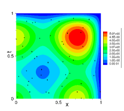
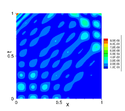
(a) (b)

Figure 7: Inverse Sine-Gordan problem: distributions of (a) the VarPro-F2 solution for $u(x,t)$ and (b) its point-wise absolute error, with the measurement points shown as “+” symbols in (a). Single sub-domain, NN $[2,300,1]$, $Q=25\times 25$, $Q_{s}=50$, $R_{m}=1.3$, $\lambda_{mea}$=1, $\epsilon=0$ (no noise in measurement data).

Figure 7 shows distributions of the $u(x,t)$ solution and its point-wise absolute error in $\Omega$ obtained by the VarPro-F2 algorithm, with $50$ random measurement points (no noise). The other parameter values are provided in the figure caption. We can observe a high accuracy in the solution, with the maximum error on the order of $10^{-8}$ in the domain. In this simulation the relative errors for the computed $\alpha_{1}$, $\alpha_{2}$ and $\alpha_{3}$ are $2.07\times 10^{-10}$, $7.54\times 10^{-9}$ and $2.39\times 10^{-8}$, respectively.

$M$	$\alpha_{1}$	$\alpha_{2}$	$\alpha_{3}$
50	-3.525085809204E+1	-6.376776028198E+0	6.877670126056E+1
100	1.006414746681E+0	9.536423027578E-1	1.058573631607E+0
200	1.000000694463E+0	9.999830213887E-1	1.000056517879E+0
300	9.999999995066E-1	1.000000013620E+0	9.999999510014E-1
400	1.000000000001E+0	9.999999999962E-1	1.000000000096E+0

Table 24: Inverse Sine-Gordan problem: $\alpha_{i}$ ($i=1,2,3$) versus $M$ (number of training parameters) obtained by the NLLSQ algorithm. Single sub-domain, NN $[2,M,1]$, $Q=25\times 25$, $Q_{s}=100$, $R_{m}=1.5$, $\lambda_{mea}$=1, $\epsilon$=0.

		NLLSQ			VarPro-F1			VarPro-F2
$M$	$e_{\alpha_{1}}$	$e_{\alpha_{2}}$	$e_{\alpha_{3}}$	$e_{\alpha_{1}}$	$e_{\alpha_{2}}$	$e_{\alpha_{3}}$	$e_{\alpha_{1}}$	$e_{\alpha_{2}}$	$e_{\alpha_{3}}$
50	3.63E+1	7.38E+0	6.78E+1	3.30E+1	6.51E+1	7.86E+0	4.55E+1	1.32E+2	4.14E+2
100	6.41E-3	4.64E-2	5.86E-2	1.76E-4	8.88E-3	1.14E-2	1.76E-4	8.88E-3	1.14E-2
200	6.94E-7	1.70E-5	5.65E-5	1.37E-7	4.34E-6	1.77E-5	1.37E-7	4.35E-6	1.77E-5
300	4.93E-10	1.36E-8	4.90E-8	2.92E-13	1.90E-10	9.64E-10	1.31E-10	1.99E-9	7.19E-9
400	1.43E-12	3.81E-12	9.58E-11	2.44E-12	3.67E-11	7.65E-11	3.31E-13	4.30E-12	7.85E-11
500	3.30E-13	7.76E-12	5.40E-11	2.84E-13	1.04E-11	4.73E-11	9.83E-13	5.90E-12	3.99E-11

Table 25: Inverse Sine-Gordan problem: $\alpha_{1}$, $\alpha_{2}$ and $\alpha_{3}$ relative errors versus $M$ obtained by the NLLSQ, VarPro-F1 and VarPro-F2 algorithms. Single sub-domain, NN $[2,M,1]$, $Q_{s}=100$, $Q=25\times 25$, $\lambda_{mea}$=1, $\epsilon$=0; $R_{m}=1.5$ with NLLSQ, $R_{m}=1.3$ with VarPro-F1 and VarPro-F2.

	NLLSQ		VarPro-F1		VarPro-F2
$M$	$l^{\infty}$-u	$l^{2}$-u	$l^{\infty}$-u	$l^{2}$-u	$l^{\infty}$-u	$l^{2}$-u
50	1.45E+0	4.90E-1	1.30E+0	4.10E-1	1.48E+0	4.85E-1
100	2.66E-2	5.24E-3	1.07E-2	2.23E-3	1.07E-2	2.23E-3
200	5.36E-6	6.69E-7	1.30E-6	2.90E-7	1.30E-6	2.90E-7
300	6.01E-9	4.75E-10	7.86E-10	9.21E-11	5.21E-9	3.44E-10
400	6.29E-11	3.77E-12	6.43E-11	4.25E-12	5.94E-10	8.53E-11
500	2.67E-11	1.13E-12	2.67E-11	1.10E-12	3.05E-10	2.08E-11

Table 26: Inverse Sine-Gordan problem: $u$ relative errors versus $M$ obtained by the NLLSQ, VarPro-F1 and VarPro-F2 algorithms. Simulation settings and parameters follow those of Table 25.

The convergence of the simulation results obtained by the NLLSQ, VarPro-F1 and VarPro-F2 algorithms is demonstrated by the data in Tables 24 to 26. In these tests the number of training parameters ($M$) is varied systematically (no noise in measurement), while the other simulation parameters are fixed and their values are provided in the table captions. Table 24 lists the computed $\alpha_{i}$ ($i=1,2,3$) values by the NLLSQ algorithm corresponding to a set of $M$. Table 25 lists the relative errors of $\alpha_{1}$, $\alpha_{2}$ and $\alpha_{3}$ computed by NLLSQ, VarPro-F1 and VarPro-F2 corresponding to different $M$. Table 26 shows the $l^{\infty}$ and $l^{2}$ norms of the relative error for $u(x,t)$ in this set of simulations. It is evident that the errors decrease exponentially with increasing number of training parameters with these algorithms.

		NLLSQ			VarPro-F1			VarPro-F2
$\epsilon$	$e_{\alpha_{1}}$	$e_{\alpha_{2}}$	$e_{\alpha_{3}}$	$e_{\alpha_{1}}$	$e_{\alpha_{2}}$	$e_{\alpha_{3}}$	$e_{\alpha_{1}}$	$e_{\alpha_{2}}$	$e_{\alpha_{3}}$
0.0	1.93E-12	4.90E-11	1.35E-10	1.50E-12	4.42E-12	2.23E-11	3.61E-11	9.72E-10	3.02E-9
0.001	6.90E-4	2.66E-3	3.00E-3	6.88E-4	2.64E-3	3.09E-3	6.86E-4	2.63E-3	3.08E-3
0.005	3.44E-3	1.31E-2	1.45E-2	3.44E-3	1.32E-2	1.54E-2	3.43E-3	1.32E-2	1.54E-2
0.01	6.88E-3	2.63E-2	2.93E-2	6.86E-3	2.63E-2	3.08E-2	6.84E-3	2.62E-2	3.04E-2
0.05	3.38E-2	1.27E-1	1.39E-1	3.38E-2	1.30E-1	1.53E-1	3.39E-2	1.32E-1	1.60E-1
0.1	6.65E-2	2.49E-1	2.76E-1	6.65E-2	2.55E-1	3.05E-1	6.65E-2	2.57E-1	3.12E-1
0.5	2.67E-1	8.07E-1	5.90E-1	2.65E-1	7.69E-1	4.39E-1	2.66E-1	7.95E-1	5.41E-1
1.0	4.09E-1	1.01E+0	2.18E-1	4.12E-1	1.07E+0	5.43E-1	4.15E-1	1.10E+0	6.27E-1

Table 27: Inverse Sine-Gordan problem: $\alpha_{1}$, $\alpha_{2}$ and $\alpha_{3}$ relative errors versus the noise level ($\epsilon$) obtained by the NLLSQ, VarPro-F1 and VarPro-F2 algorithms. Single sub-domain, NN: $[2,400,1]$, $Q=30\times 30$, $Q_{s}=50$, $\lambda_{mea}$=1; $R_{m}=1.5$ with NLLSQ, $R_{m}=1.3$ with VarPro-F1 and VarPro-F2;

	NLLSQ		VarPro-F1		VarPro-F2
$\epsilon$	$l^{\infty}$-u	$l^{2}$-u	$l^{\infty}$-u	$l^{2}$-u	$l^{\infty}$-u	$l^{2}$-u
0.0	3.44E-11	4.16E-12	7.03E-11	5.01E-12	7.73E-10	1.57E-10
0.001	8.76E-4	3.71E-4	8.49E-4	3.70E-4	8.51E-4	3.69E-4
0.005	4.39E-3	1.86E-3	4.26E-3	1.85E-3	4.25E-3	1.85E-3
0.01	8.77E-3	3.71E-3	8.50E-3	3.70E-3	8.51E-3	3.70E-3
0.05	4.35E-2	1.87E-2	4.25E-2	1.87E-2	4.24E-2	1.86E-2
0.1	8.65E-2	3.78E-2	8.46E-2	3.77E-2	8.43E-2	3.76E-2
0.5	4.10E-1	1.95E-1	4.08E-1	1.95E-1	4.07E-1	1.95E-1
1.0	8.90E-1	3.83E-1	8.97E-1	3.84E-1	9.07E-1	3.86E-1

Table 28: Inverse Sine-Gordan problem: $u$ relative errors versus $\epsilon$ obtained by the NLLSQ, VarPro-F1 and VarPro-F2 algorithms. Simulation settings and parameters follow those of Table 27.

The effect of noise in the measurement data on the simulation accuracy is illustrated by Tables 27 and 28 for the NLLSQ, VarPro-F1 and VarPro-F2 algorithms. The relative errors of $\alpha_{1}$, $\alpha_{2}$, $\alpha_{3}$, and $u(x,t)$ corresponding to a range of noise levels are provided in these two tables. The other crucial simulation parameters are provided in the caption of Table 27. The accuracy in the computation results deteriorates as the measurement data becomes more noisy. With $1\%$ measurement noise ($\epsilon=0.01$) the relative errors of the computed $\alpha_{i}$ ($i=1,2,3$) are around $0.7\sim 3\%$, and the relative error of $u$ ($l^{2}$ norm) is around $0.4\%$ with the three algorithms. With $5\%$ measurement noise ($\epsilon=0.05$) the relative errors of the computed $\alpha_{i}$ are around $3\sim 15\%$ and the relative error of $u$ ($l^{2}$ norm) is less than $2\%$.

3.6 Helmholtz Equation with Inverse Variable Coefficient

In the last example, we use our method to study a problem involving an inverse coefficient field. Consider the domain $(x,y)\in\Omega=[0,1.5]\times[0,1.5]$ and the inverse problem on $\Omega$,

$$\frac{\partial^{2}u}{\partial x^{2}}+\frac{\partial^{2}u}{\partial y^{2}}-\gamma(x,y)u=f(x,y),$$ (64a)

$$u(a_{1},y)=g_{1}(y),\quad u(b_{1},y)=g_{2}(y),\quad u(x,a_{2})=g_{3}(x),\quad u(x,b_{2})=g_{4}(x),$$ (64b)

$$u(\xi_{i},\eta_{i})=S(\xi_{i},\eta_{i}),\quad(\xi_{i},\eta_{i})\in\mathbb{Y}\subset\Omega,\ 1\leqslant i\leqslant NQ_{s},$$ (64c)

where $f$ is a prescribed source term, $g_{i}$ ($1\leqslant i\leqslant 4$) denote the prescribed boundary data, $\mathbb{Y}$ is the set of measurement points, $S(\xi_{i},\eta_{i})$ denotes the measurement data at the random point $(\xi_{i},\eta_{i})$, and $\gamma(x,y)$ and $u(x,y)$ are two field functions to be determined. We employ the following manufactured solutions,

$$\small\left\{\begin{split}&\gamma_{ex}(x,y)=100\left[1+\frac{1}{4}\sin(2\pi x)+\frac{1}{4}\sin(2\pi y)\right],\\ &u_{ex}(x,y)=\left[\frac{5}{2}\sin\left(\pi x-\frac{2\pi}{5}\right)+\frac{3}{2}\cos\left(2\pi x+\frac{3\pi}{10}\right)\right]\left[\frac{5}{2}\sin\left(\pi y-\frac{2\pi}{5}\right)+\frac{3}{2}\cos\left(2\pi y+\frac{3\pi}{10}\right)\right].\end{split}\right.$$ (65)

$f$ and $g_{i}$ ($1\leqslant i\leqslant 4$) are chosen accordingly such that the expressions in (65) satisfy the equations (64a)–(64b). The measurement data $S(\xi_{i},\eta_{i})$ are given by equation (54), in which the $u_{ex}$ is given in (65). The relative errors for $u(x,y)$ are defined in (55), and the relative errors for $\gamma(x,y)$ are defined analogously. The $\gamma(x,y)$ and $u(x,y)$ errors reported below are computed on a uniform $Q_{eval}=101\times 101$ grid in each sub-domain. The notations here follow those of previous subsections.

We employ the algorithm modification as outlined in Remark 2.7 for solving this problem. Compared with previous subsections, the main change here lies in that the local neural network on each sub-domain contains two nodes in the output layer, one representing $u(x,y)$ and the other $\gamma(x,y)$. The output-layer coefficients contributing to $\gamma(x,y)$ play the role of the inverse parameters. We also find it preferable to regularize the the output-layer coefficients that contribute to $\gamma(x,y)$ (or $u(x,y)$) for this problem. For regularization we employ the extra terms for the underlying loss function, $\frac{\lambda_{1}^{2}}{2}\|\bm{\alpha}\|^{2}+\frac{\lambda_{2}^{2}}{2}\|\bm{\beta}\|^{2}$, where $\bm{\alpha}$ and $\bm{\beta}$ denote the vectors of output-layer coefficients for $\gamma(x,y)$ and $u(x,y)$, respectively, and the prescribed non-negative constants $\lambda_{1}$ and $\lambda_{2}$ are the corresponding regularization coefficients.

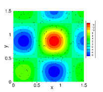
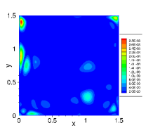
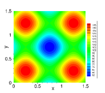
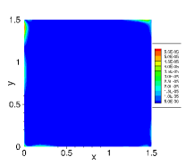
(a) (b) (c) (d)

Figure 8: Inverse variable-coefficient Helmholtz problem: distributions of (a) the NLLSQ solution for $u(x,y)$ and (b) its point-wise absolute error, (c) the NLLSQ solution for $\gamma(x,y)$ and (d) its point-wise absolute error, with the $Q_{s}=300$ random measurement points shown in (a) as “+” symbols. Single sub-domain, NN $[2,400,1]$, $Q=30\times 30$, $R_{m}=1.5$, $\lambda_{mea}=1$, $\epsilon=0$ (no noise), $\lambda_{1}=\lambda_{2}=0$ (no regularization).

Figure 8 shows distributions of the solutions for $u(x,y)$ and $\gamma(x,y)$, and their point-wise absolute errors, obtained by the NLLSQ algorithm. The random measurement points are also shown in Figure 8(a). The figure caption lists the main parameter values for this simulation. We observe a fairly high accuracy, with the maximum $u$ error on the order of $10^{-8}$ and the maximum $\gamma$ error on the order of $10^{-5}$ in the domain.

			$l^{\infty}$-$\gamma$	$l^{2}$-$\gamma$	$l^{\infty}$-u	$l^{2}$-u
collocation	$Q=$	5$\times$5	9.84E-2	3.15E-2	7.94E-3	4.38E-4
point test		10$\times$10	4.05E-3	2.90E-4	1.63E-4	1.02E-5
		15$\times$15	1.15E-4	4.94E-6	3.38E-6	2.99E-7
		20$\times$20	4.99E-6	4.84E-7	2.65E-7	2.70E-8
		25$\times$25	4.42E-6	3.57E-7	3.34E-7	2.90E-8
		30$\times$30	1.56E-6	1.46E-7	1.19E-7	1.08E-8
		35$\times$35	1.61E-6	1.73E-7	1.26E-7	1.15E-8
training	$M=$	50	6.79E+0	1.67E+0	1.63E+0	5.67E-1
parameter		100	8.64E-2	1.10E-2	8.44E-3	2.00E-3
test		200	1.98E-4	2.08E-5	6.46E-6	6.42E-7
		300	2.07E-6	1.26E-7	3.13E-8	2.46E-9
		400	5.08E-7	2.95E-8	5.76E-9	5.29E-10
		500	1.61E-7	1.18E-8	1.95E-9	1.91E-10
measurement	$Q_{s}=$	10	1.36E-3	3.11E-4	2.49E-4	6.60E-5
point test		30	1.93E-4	3.69E-5	2.03E-5	4.24E-6
		50	2.69E-5	4.08E-6	2.03E-6	3.83E-7
		100	3.18E-6	2.95E-7	2.25E-7	1.78E-8
		200	5.30E-6	2.53E-7	8.21E-8	5.48E-9
		300	1.45E-6	9.93E-8	2.45E-8	2.00E-9
		400	2.65E-6	8.80E-8	1.40E-8	1.79E-9
noise level	$\epsilon=$	0.0	1.61E-6	1.73E-7	1.26E-7	1.15E-8
test		0.0005	5.15E-2	5.54E-3	3.32E-3	4.54E-4
		0.001	7.57E-2	7.31E-3	5.46E-3	6.63E-4
		0.005	2.69E-1	2.92E-2	2.28E-2	3.12E-3
		0.01	4.26E-1	4.96E-2	3.94E-2	5.98E-3
		0.05	1.50E+0	2.00E-1	1.44E-1	2.71E-2
		0.1	1.85E+0	2.97E-1	2.26E-1	4.97E-2

Table 29: Inverse variable-coefficient Helmholtz problem: relative $l^{\infty}$ and $l^{2}$ errors of $\gamma(x,y)$ and $u(x,y)$ in several tests with the NLLSQ algorithm. Single sub-domain, NN $[2,M,1]$. In collocation point test, $M=400$, $Q_{s}=100$, $\epsilon=0$, $Q$ is varied. In training parameter test, $Q=30\times 30$, $Q_{s}=300$, $\epsilon=0$, $M$ is varied. In measurement point test, $Q=25\times 25$, $M=300$, $\epsilon=0$, $Q_{s}$ is varied. In noise level test, $Q=35\times 35$, $M=400$, $Q_{s}=100$, $\epsilon$ is varied. $R_{m}=1.5$ and $\lambda_{mea}=1$ in all tests. No regularization ($\lambda_{1}=\lambda_{2}=0$).

Table 29 lists the relative errors for $\gamma$ and $u$ ($l^{\infty}$ and $l^{2}$ norms) computed by the NLLSQ algorithm in several sets of tests, with respect to $Q$ (number of collocation points), $M$ (number of training parameters), $Q_{s}$ (number of random measurement points), and $\epsilon$ (noise level). The settings and the simulation parameter values are provided in the table caption for each set of tests. One can observe an approximately exponential decrease in the $\gamma$ and $u$ errors with respect to $Q$, $M$ and $Q_{s}$ (before saturation). One can also observe the deterioration in the simulation accuracy with increasing noise level in the measurement data. Note that no regularization is employed in these simulations. The noise appears to affect the $\gamma$ results more significantly than $u$. For example, with $1\%$ noise ($\epsilon=0.01$) in the measurement data, the maximum ($l^{\infty}$) relative error for $\gamma(x,y)$ is around $43\%$ and the $l^{2}$ relative error is around $5\%$, while for $u(x,y)$ these errors are around $4\%$ and $0.6\%$ respectively.

	noise	level	$l^{\infty}$-$\gamma$	$l^{2}$-$\gamma$	$l^{\infty}$-u	$l^{2}$-u
NLLSQ	$\epsilon=$	0.0	1.39E-4	7.11E-6	2.57E-6	2.24E-7
		0.0005	1.47E-2	1.42E-3	7.48E-4	2.17E-4
		0.001	2.92E-2	2.85E-3	1.50E-3	4.34E-4
		0.005	1.27E-1	1.36E-2	7.33E-3	2.17E-3
		0.01	2.14E-1	2.58E-2	1.48E-2	4.32E-3
		0.05	7.38E-1	1.02E-1	7.35E-2	2.14E-2
		0.1	8.43E-1	1.84E-1	1.48E-1	4.26E-2
VarPro-F1	$\epsilon=$	0.0	3.16E-4	3.02E-5	7.75E-6	1.11E-6
		0.0005	1.65E-2	1.93E-3	7.23E-4	2.18E-4
		0.001	3.21E-2	3.81E-3	1.44E-3	4.35E-4
		0.005	1.30E-1	1.78E-2	7.29E-3	2.16E-3
		0.01	2.31E-1	3.34E-2	1.48E-2	4.31E-3
		0.05	9.30E-1	1.16E-1	7.19E-2	2.14E-2
		0.1	1.02E+0	2.08E-1	1.42E-1	4.29E-2
VarPro-F2	$\epsilon=$	0.0	5.71E-4	4.93E-5	1.28E-5	1.29E-6
		0.0005	2.18E-2	2.46E-3	7.19E-4	2.23E-4
		0.001	4.33E-2	4.90E-3	1.44E-3	4.46E-4
		0.005	1.88E-1	2.30E-2	6.97E-3	2.21E-3
		0.01	3.37E-1	4.42E-2	1.37E-2	4.39E-3
		0.05	1.60E+0	1.93E-1	6.91E-2	2.18E-2
		0.1	2.66E+0	3.11E-1	1.38E-1	4.31E-2

Table 30: Inverse variable-coefficient Helmholtz problem: relative $l^{\infty}$ and $l^{2}$ errors of $\gamma(x,y)$ and $u(x,y)$ versus $\epsilon$ (noise level) by the NLLSQ, VarPro-F1 and VarPro-F2 algorithms. Single sub-domain, NN [2,400,1], $Q=30\times 30$, $Q_{s}=300$, $\lambda_{mea}=1$; $R_{m}=1.5$ with NLLSQ, $R_{m}=2.5$ with VarPro-F1, $R_{m}=3.0$ with VarPro-F2; Regularization coefficients: $(\lambda_{1},\lambda_{2})=(1E-8,1E-8)$ with NLLSQ, $(\lambda_{1},\lambda_{2})=(1E-7,0)$ with VarPro-F1, and $(\lambda_{1},\lambda_{2})=(1E-6,0)$ with VarPro-F2.

Table 30 illustrates the effect of noise in the measurement data on the accuracy of the NLLSQ, VarPro-F1 and VarPro-F2 algorithms. The relative errors for $\gamma$ and $u$ corresponding to different noise levels have been shown. In these simulations the output-layer coefficients for $\gamma(x,y)$ (and also for $u(x,y)$ with NLLSQ) have been regularized, with the regularization coefficients and the other simulation parameter values given in the table caption. The regularization generally improves the accuracy in the presence of noise.

4 Concluding Remarks

In this paper we have presented a method for solving inverse parametric PDE problems based on randomized neural networks. This method extends the local extreme learning machine (locELM) technique to inverse PDEs. The field solution is represented by a set of local random-weight neural networks (randomly assigned but fixed hidden-layer coefficients, trainable output-layer coefficients), one for each sub-domain. The local neural networks are coupled through the $C^{k}$ (with $k$ related to the PDE order) continuity conditions on the shared sub-domain boundaries. The inverse parameters of the PDE and the trainable parameters of the local neural networks are the unknowns to be determined in the system.

Three algorithms are developed for training the neural network to solve the inverse problem. The first algorithm (NLLSQ) computes the inverse parameters and the trainable network parameters all together by the nonlinear least squares method and is an extension of the nonlinear least squares method with perturbations (NLLSQ-perturb) of DongL2021 (developed for forward PDEs) to inverse PDE problems. The second and the third algorithms are based on the variable projection idea. The second algorithm (VarPro-F1) employs variable projection to eliminate the inverse parameters from the problem and attain a reduced problem about the trainable network parameters only. Then the reduced problem is solved first by the NLLSQ-perturb algorithm for the trainable network parameters, and the inverse parameters are computed afterwards by the linear least squares method. The third algorithm (VarPro-F2) provides a reciprocal formulation with variable projection. It eliminates the trainable network parameters (or equivalently the field solution) from the problem first to arrive at a reduced problem about the inverse parameters only. Then the inverse parameters are computed first by solving the reduced problem with the NLLSQ-perturb algorithm, and afterwards the trainable network parameters are computed based on the inverse parameters already obtained. The VarPro-F2 algorithm is suitable for parametric PDEs that are linear with respect to the field solution. For PDEs that are nonlinear with respect to the field solution, this algorithm needs to be combined with a Newton iteration.

The presented method is numerically tested using several inverse parametric PDE problems. It is also compared with the PINN method (see Appendix C). For smooth solutions and noise-free data, the errors for the inverse parameters and the field solution computed by the NLLSQ, VarPro-F1 and VarPro-F2 algorithms decrease exponentially with respect to the number of collocation points and the number of training parameters in the neural network. When these parameters become large the errors can reach a level close to the machine accuracy. These characteristics are in some sense analogous to those observed for the forward PDE problems in DongL2021 ; DongY2022rm . For noisy measurement data, these algorithms can produce computation results with good accuracy, indicating robustness of the method. We observe that, in the presence of noise, by scaling the measurement residual by a factor $\lambda_{mea}$ ($0<\lambda_{mea}<1$) one can in general improve the simulation accuracy of the current method markedly, while this scaling only slightly degrades the accuracy for the noise-free data. The comparison with PINN shows that the current method has an advantage in terms of both accuracy and the network training time. In particular, for the noise-free data the current method exhibits an accuracy significantly higher than PINN.

These test results suggest that the method developed herein is an effective and promising technique for computing inverse PDEs. The exponential convergence exhibited by the method is especially interesting, suggesting a high accuracy of this technique. We anticipate that this technique will be a useful and meaningful addition to the arsenal for tackling this class of problems and be instrumental in computational science and engineering applications.

Appendix A. Nonlinear Least Squares Algorithm with Perturbations (NLLSQ-perturb)

We summarize the nonlinear least squares algorithm with perturbations (NLLSQ-perturb) below in Algorithm 7, which is adapted from the one developed in DongL2021 with certain modifications.

1

input : max perturbation magnitude $\delta>0$; initial guess vector $\bm{\theta}_{0}$; routine for computing residual; routine for computing Jacobian matrix; perturbation flag $\eta$ (integer, $0$ or $1$); tolerance $\varepsilon>0$; max-nllsq-iterations (positive integer); max-sub-iterations (non-negative integer).

output : solution vector $\bm{\theta}$, associated cost $c$

2 invoke the scipy.optimize.least_squares routine, with the inputs (initial guess $\bm{\theta}_{0}$, routines for residual/jacobian-matrix calculations, and max-nllsq-iterations)

3 set $\bm{\theta}\leftarrow$ returned solution, and set $c\leftarrow$ returned cost

4 if c is below $\varepsilon$ then

5      return $\bm{\theta}$ and $c$

6 end if

7for $i\leftarrow 1$ to max-sub-iterations do

8       generate a uniform random number $\xi$ on the interval $[0,1]$

9       set $\delta_{1}\leftarrow\xi\delta$

10       generate a uniform random vector $\Delta\bm{\theta}$ of the same shape as $\bm{\theta}$ on the interval [$-\delta_{1}$, $\delta_{1}$]

11       if $\eta$ is $0$ then

12             $\bm{\vartheta}_{0}\leftarrow\Delta\bm{\theta}$

13            

14      else

15            $\bm{\vartheta}_{0}\leftarrow\bm{\theta}+\Delta\bm{\theta}$

16            

17       end if

18      invoke the scipy.optimize.least_squares routine, with the inputs (initial guess $\bm{\vartheta}_{0}$, routines for residual/jacobian-matrix calculations, and max-nllsq-iterations)

19       if the returned cost is less than $c$ then

20             set $\bm{\theta}\leftarrow$ the returned solution, and set $c\leftarrow$ the returned cost

21             if c is below $\varepsilon$ then

22                   break

23                  

24             end if

25            

26       end if

27      

28 end for

29return $\bm{\theta}$ and $c$

Algorithm 7 NLLSQ-perturb (nonlinear least squares with perturbations) algorithm

In this algorithm, $\delta$ controls the maximum magnitude of each component of the random perturbation vector $\Delta\bm{\theta}$. The vector $\bm{\theta}_{0}$ provides the initial guess to the solution of the nonlinear least squares problem. If the returned solution from the scipy least_squares() routine corresponding to $\bm{\theta}_{0}$ is not acceptable (i.e. the returned cost exceeding the tolerance $\varepsilon$), then a sub-iteration procedure is triggered in which new initial guesses ($\bm{\vartheta}_{0}$) are generated by perturbing either the origin or the best approximation to the solution obtained so far with a random vector. The scipy least_squares() routine is invoked with the new initial guesses until an acceptable solution is obtained or until the maximum number of sub-iterations is reached. The integer flag $\eta$ controls around which point the perturbation is performed. If $\eta=0$ the new initial guess is generated by perturbing the origin. Otherwise, the current best approximation to the solution is perturbed to generate a new initial guess. The parameter “max-nllsq-iterations” controls the maximum number of iterations (e.g. the maximum number of residual function evaluations) in the scipy least_squares() routine. The parameter “max-sub-iterations” controls the maximum number of sub-iterations for the initial guess perturbation. One can turn off the perturbation in the NLLSQ-perturb algorithm by setting max-sub-iterations to zero. Note that the scipy least_squares() function requires two routines in the input, one for computing the residual and the other for computing the Jacobian matrix for an arbitrary given approximation to the solution.

Appendix B. Matrices in the VarPro-F2 Algorithm

The matrices in the expressions (44) are given by,

$$\footnotesize\begin{split}&\mathbf{b}^{\text{pde}}=\begin{bmatrix}\vdots\\ f(\mathbf{x}_{p}^{e})\\ \vdots\end{bmatrix}_{NQ\times 1},\ \mathbf{b}^{\text{mea}}=\begin{bmatrix}\vdots\\ S(\bm{\xi}_{p}^{e})\\ \vdots\end{bmatrix}_{NQ_{s}\times 1},\ \mathbf{b}^{\text{bc1}}=\begin{bmatrix}\vdots\\ g(a_{1},y_{p(1,j)}^{e(1,l)})\\ \vdots\end{bmatrix}_{N_{2}Q_{2}\times 1},\\ &\mathbf{b}^{\text{bc2}}=\begin{bmatrix}\vdots\\ g(b_{1},y_{p(Q_{1},j)}^{e(N_{1},l)})\\ \vdots\end{bmatrix}_{N_{2}Q_{2}\times 1},\ \mathbf{b}^{\text{bc3}}=\begin{bmatrix}\vdots\\ g(x_{p(i,1)}^{e(m,1)},a_{2})\\ \vdots\end{bmatrix}_{N_{1}Q_{1}\times 1},\ \mathbf{b}^{\text{bc4}}=\begin{bmatrix}\vdots\\ g(x_{p(i,Q_{2})}^{e(m,N_{2})},a_{2})\\ \vdots\end{bmatrix}_{N_{1}Q_{1}\times 1},\\ &\mathbf{H}^{\text{pde}}=\begin{bmatrix}h_{ij}^{\text{pde}}\end{bmatrix}_{NQ\times NM},\ \mathbf{H}^{\text{mea}}=\begin{bmatrix}h_{ij}^{\text{mea}}\end{bmatrix}_{NQ_{s}\times NM},\ \mathbf{H}^{\text{bc1}}=\begin{bmatrix}h_{ij}^{\text{bc1}}\end{bmatrix}_{N_{2}Q_{2}\times NM},\ \mathbf{H}^{\text{bc2}}=\begin{bmatrix}h_{ij}^{\text{bc2}}\end{bmatrix}_{N_{2}Q_{2}\times NM},\\ &\mathbf{H}^{\text{bc3}}=\begin{bmatrix}h_{ij}^{\text{bc3}}\end{bmatrix}_{N_{1}Q_{1}\times NM},\ \mathbf{H}^{\text{bc4}}=\begin{bmatrix}h_{ij}^{\text{bc4}}\end{bmatrix}_{N_{1}Q_{1}\times NM},\ \mathbf{H}^{\text{ck1}}=\begin{bmatrix}h_{ij}^{\text{ck1}}\end{bmatrix}_{(N-N_{2})Q_{2}\times NM},\\ &\mathbf{H}^{\text{ck2}}=\begin{bmatrix}h_{ij}^{\text{ck2}}\end{bmatrix}_{(N-N_{2})Q_{2}\times NM},\ \mathbf{H}^{\text{ck3}}=\begin{bmatrix}h_{ij}^{\text{ck3}}\end{bmatrix}_{(N-N_{1})Q_{1}\times NM},\ \mathbf{H}^{\text{ck4}}=\begin{bmatrix}h_{ij}^{\text{ck4}}\end{bmatrix}_{(N-N_{1})Q_{1}\times NM}.\end{split}$$ (66)

In the matrices $\mathbf{H}^{\text{pde}}$ and $\mathbf{H}^{\text{mea}}$ the only non-zero terms are,

$$\footnotesize\left\{\begin{split}h_{ij}^{\text{pde}}=&\alpha_{1}\mathcal{L}_{1}\phi_{eq}(\mathbf{x}_{p}^{e})+\dots+\alpha_{n}\mathcal{L}_{n}\phi_{eq}(\mathbf{x}_{p}^{e})+\mathcal{F}\phi_{eq}(\mathbf{x}_{p}^{e}),\\ &i=(e-1)Q+p,\ j=(e-1)M+q,\quad\text{for}\ 1\leqslant(e,p,q)\leqslant(N,Q,M);\\ h_{ij}^{\text{mea}}=&\mathcal{M}\phi_{eq}(\bm{\xi}_{p}^{e}),\ \ i=(e-1)Q_{s}+p,\ j=(e-1)M+q,\quad\text{for}\ 1\leqslant(e,p,q)\leqslant(N,Q_{s},M).\end{split}\right.$$ (67)

In the matrices $\mathbf{H}^{\text{bc1}}$, $\mathbf{H}^{\text{bc2}}$, $\mathbf{H}^{\text{bc3}}$ and $\mathbf{H}^{\text{bc4}}$ the only non-zero terms are,

$$\footnotesize\left\{\begin{split}h_{ij}^{\text{bc1}}=&\mathcal{B}\phi_{eq}(a_{1},y_{p}^{e}),\ e=e(1,l),\ p=p(1,k),\ i=(l-1)Q_{2}+k,\ j=(e-1)M+q,\ \text{for}\ 1\leqslant(l,k)\leqslant(N_{2},Q_{2});\\ h_{ij}^{\text{bc2}}=&\mathcal{B}\phi_{eq}(b_{1},y_{p}^{e}),\ e=e(N_{1},l),\ p=p(Q_{1},k),\ i=(l-1)Q_{2}+k,\ j=(e-1)M+q,\ \text{for}\ 1\leqslant(l,k)\leqslant(N_{2},Q_{2});\\ h_{ij}^{\text{bc3}}=&\mathcal{B}\phi_{eq}(x_{p}^{e},a_{2}),\ e=e(m,1),\ p=p(k,1),\ i=(m-1)Q_{1}+k,\ j=(e-1)M+q,\ \text{for}\ 1\leqslant(m,k)\leqslant(N_{1},Q_{1});\\ h_{ij}^{\text{bc4}}=&\mathcal{B}\phi_{eq}(x_{p}^{e},b_{2}),\ e=e(m,N_{2}),\ p=p(k,Q_{2}),\ i=(m-1)Q_{1}+k,\ j=(e-1)M+q,\ \text{for}\ 1\leqslant(m,k)\leqslant(N_{1},Q_{1}),\end{split}\right.$$ (68)

where the functions $e(\cdot,\cdot)$ and $p(\cdot,\cdot)$ are given by (7) and (10). In the matrices $\mathbf{H}^{\text{ck1}}$, $\mathbf{H}^{\text{ck2}}$, $\mathbf{H}^{\text{ck3}}$ and $\mathbf{H}^{\text{ck4}}$ the only non-zero terms are,

$$\footnotesize\left\{\begin{split}h_{ij_{1}}^{\text{ck1}}=&\phi_{e_{1}q}(X_{m},y_{p_{1}}^{e_{1}}),\ h_{ij_{2}}^{\text{ck1}}=-\phi_{e_{2}q}(X_{m},y_{p_{2}}^{e_{2}}),\ e_{1}=e(m,l),\ p_{1}=p(Q_{1},k),\ e_{2}=e(m+1,l),\\ &p_{2}=p(1,k),\ i=(m-1)N_{2}Q_{2}+(l-1)Q_{2}+k,\ j_{1}=(e_{1}-1)M+q,\ j_{2}=(e_{2}-1)M+q,\\ &\text{for}\ 1\leqslant(m,l,k,q)\leqslant(N_{1}-1,N_{2},Q_{2},M);\\ h_{ij_{1}}^{\text{ck2}}=&\left.\frac{\partial\phi_{e_{1}q}}{\partial x}\right|_{(X_{m},y_{p_{1}}^{e_{1}})},\ h_{ij_{2}}^{\text{ck2}}=-\left.\frac{\partial\phi_{e_{2}q}}{\partial x}\right|_{(X_{m},y_{p_{2}}^{e_{2}})},\ e_{1}=e(m,l),\ p_{1}=p(Q_{1},k),\ e_{2}=e(m+1,l),\\ &p_{2}=p(1,k),\ i=(m-1)N_{2}Q_{2}+(l-1)Q_{2}+k,\ j_{1}=(e_{1}-1)M+q,\ j_{2}=(e_{2}-1)M+q,\\ &\text{for}\ 1\leqslant(m,l,k,q)\leqslant(N_{1}-1,N_{2},Q_{2},M);\\ h_{ij_{1}}^{\text{ck3}}=&\phi_{e_{1}q}(x_{p_{1}}^{e_{1}},Y_{l}),\ h_{ij_{2}}^{\text{ck3}}=-\phi_{e_{2}q}(x_{p_{2}}^{e_{2}},Y_{l}),\ e_{1}=e(m,l),\ p_{1}=p(k,Q_{2}),\ e_{2}=e(m,l+1),\\ &p_{2}=p(k,1),\ i=(l-1)N_{1}Q_{1}+(m-1)Q_{1}+k,\ j_{1}=(e_{1}-1)M+q,\ j_{2}=(e_{2}-1)M+q,\\ &\text{for}\ 1\leqslant(m,l,k,q)\leqslant(N_{1},N_{2}-1,Q_{1},M);\\ h_{ij_{1}}^{\text{ck4}}=&\left.\frac{\partial\phi_{e_{1}q}}{\partial y}\right|_{(x_{p_{1}}^{e_{1}},Y_{l})},\ h_{ij_{2}}^{\text{ck4}}=-\left.\frac{\partial\phi_{e_{2}q}}{\partial y}\right|_{(x_{p_{2}}^{e_{2}},Y_{l})},\ e_{1}=e(m,l),\ p_{1}=p(k,Q_{2}),\ e_{2}=e(m,l+1),\\ &p_{2}=p(k,1),\ i=(l-1)N_{1}Q_{1}+(m-1)Q_{1}+k,\ j_{1}=(e_{1}-1)M+q,\ j_{2}=(e_{2}-1)M+q,\\ &\text{for}\ 1\leqslant(m,l,k,q)\leqslant(N_{1},N_{2}-1,Q_{1},M).\end{split}\right.$$ (69)

Appendix C. Comparison with PINN

This appendix provides a comparison of the simulation results obtained by the current method (NLLSQ algorithm) and the physics-informed neural network (PINN) method RaissiPK2019 for several test problems from Section 3. The PINN method is also implemented in Python based on the Tensorflow and Keras libraries. The PINN loss function consists of those contributions from the parametric PDE, the measurement, and the boundary/initial conditions (BC/IC). Let $\gamma_{bc}\in(0,1)$ denote the penalty coefficient in front of the BC/IC loss term, and we employ $(1-\gamma_{bc})$ as the penalty coefficient for the PDE and measurement loss terms. We have varied $\gamma_{bc}$, the learning rate schedule, and the random initialization for the weights/biases of PINN systematically. PINN is trained by the Adam optimizer. The PINN/Adam results reported below are the best we have obtained for these problems using PINN. We have also tried the L-BFGS optimizer with PINN, and its results for these inverse problems are quite poor and worse than the Adam results.

		$\epsilon$=0				$\epsilon$=0.01
method	$e_{\alpha}$	$l^{\infty}$-u	$l^{2}$-u	time(sec)	$e_{\alpha}$	$l^{\infty}$-u	$l^{2}$-u	time(sec)
PINN (Adam)	6.31E-3	1.08E-2	3.56E-3	134.5	5.53E-3	1.03E-2	3.30E-3	130.9
current (NLLSQ)	1.66E-8	3.66E-6	2.62E-7	11.5	9.72E-4	1.76E-3	5.26E-4	10.4

Table 31: Inverse Poisson problem: relative errors of $\alpha$ and $u$ and the network training time (seconds) obtained by PINN (Adam) and the current NLLSQ algorithm. In both PINN and NLLSQ, Q=30$\times$30, $Q_{s}$=100, Gaussian activation function. In PINN, neural network $[2,30,30,30,1]$; $20,000$ training epochs; $\gamma_{bc}=0.99$; learning rate decreasing linearly from 0.01 to 1.0E-4 in first $10,000$ epochs, and fixed at 1.0E-4 afterwards. In NLLSQ, single sub-domain, neural network $[2,500,1]$, $R_{m}$=3.0, $\lambda_{mea}$=0.1.

		$\epsilon$=0				$\epsilon$=0.01
method	$e_{c}$	$l^{\infty}$-u	$l^{2}$-u	time(sec)	$e_{c}$	$l^{\infty}$-u	$l^{2}$-u	time(sec)
PINN (Adam)	1.18E-5	7.18E-3	7.63E-4	133.5	1.47E-4	9.15E-3	1.67E-3	134.9
current (NLLSQ)	2.32E-10	8.51E-8	4.66E-9	29.6	2.61E-5	2.85E-4	1.10E-4	39.3

Table 32: Inverse advection problem: relative errors of $c$ and $u$ and the network training time (seconds) obtained by the PINN (Adam) and the current NLLSQ algorithm. In both PINN and NLLSQ, Q=30$\times$30, $Q_{s}$=100, Gaussian activation function. In PINN, neural network $[2,30,30,30,30,1]$; $20,000$ training epochs; $\gamma_{bc}=0.2$; learning rate decreasing linearly from 0.01 to 1.0E-4 in first $10,000$ epochs, and fixed at 1.0E-4 afterwards. In NLLSQ, single sub-domain, neural network $[2,400,1]$, $R_{m}$=2.5, $\lambda_{mea}$=0.1.

noise level	method	$e_{\alpha_{1}}$	$e_{\alpha_{2}}$	$l^{\infty}$-u	$l^{2}$-u	training-time(sec)
$\epsilon=0$	PINN (Adam)	7.08E-1	2.68E-1	1.48E+0	5.65E-1	3049.2
	current (NLLSQ)	5.71E-9	3.05E-7	5.98E-8	1.49E-8	10.3
$\epsilon=0.01$	PINN (Adam)	6.74E-1	7.76E-1	1.56E+0	6.79E-1	2742.9
	current (NLLSQ)	4.34E-3	7.13E-4	5.25E-3	2.38E-3	10.0

Table 33: Inverse nonlinear Helmholtz problem: relative errors of $\alpha_{1}$, $\alpha_{2}$ and $u$ and the network training time (seconds) obtained by PINN (Adam) and the current NLLSQ algorithm. In both PINN and NLLSQ, Q=30$\times$30, $Q_{s}$=100, Gaussian activation function. In PINN, neural network $[2,30,30,30,30,30,30,1]$; $200,000$ training epochs; $\gamma_{bc}=0.99$; learning rate decreasing linearly from 0.01 to 1.0E-4 in first $10,000$ epochs, and fixed at 1.0E-4 afterwards. In NLLSQ, single sub-domain, neural network $[2,500,1]$, $R_{m}$=2.25, $\lambda_{mea}$=0.25.

noise level	method	$e_{\alpha_{1}}$	$e_{\alpha_{2}}$	$l^{\infty}$-u	$l^{2}$-u	training-time(sec)
$\epsilon=0$	PINN (Adam)	2.40E-4	7.26E-4	1.59E-3	2.06E-4	529.0
	current (NLLSQ)	4.31E-10	2.33E-9	3.31E-9	5.86E-10	4.2
$\epsilon=0.01$	PINN (Adam)	1.80E-3	2.66E-3	5.65E-3	7.83E-4	540.1
	current (NLLSQ)	1.12E-5	1.23E-4	9.87E-5	3.75E-5	6.4

Table 34: Inverse Burgers’ problem: relative errors of $\alpha_{1}$, $\alpha_{2}$ and $u$ and the network training time (seconds) obtained by PINN (Adam) and the current NLLSQ algorithm. In both PINN and NLLSQ, Q=30$\times$30, $Q_{s}$=100, Gaussian activation function. In PINN, neural network $[2,30,30,30,30,1]$; $50,000$ training epochs; $\gamma_{bc}=0.9$; learning rate decreasing linearly from 0.01 to 1.0E-4 in first $10,000$ epochs, and fixed at 1.0E-4 afterwards. In NLLSQ, single sub-domain, neural network $[2,400,1]$, $R_{m}$=1.9, $\lambda_{mea}$=0.1.

noise level	method	$e_{\alpha_{1}}$	$e_{\alpha_{2}}$	$e_{\alpha_{3}}$	$l^{\infty}$-u	$l^{2}$-u	training-time(sec)
$\epsilon=0$	PINN (Adam)	9.21E-3	2.30E-1	7.33E-1	1.86E-2	3.32E-3	1853.3
	current (NLLSQ)	7.65E-10	4.49E-9	6.60E-9	7.97E-10	3.50E-10	23.6
$\epsilon=0.01$	PINN (Adam)	1.16E-2	1.35E-1	3.51E-1	1.18E-2	2.97E-3	1833.2
	current (NLLSQ)	5.45E-3	2.59E-2	5.09E-3	5.76E-3	2.63E-3	30.1

Table 35: Inverse Sine-Gordan problem: relative errors of $\alpha_{i}$ ($i=1,2,3$) and $u$ and the network training time (seconds) obtained by PINN (Adam) and the current NLLSQ algorithm. In both PINN and NLLSQ, Q=30$\times$30, $Q_{s}$=100, Gaussian activation function. In PINN, neural network $[2,30,30,30,30,1]$; $200,000$ training epochs; $\gamma_{bc}=0.99$, learning rate decreasing linearly from 0.01 to 1.0E-4 in first $10,000$ epochs, and fixed at 1.0E-4 afterwards. In NLLSQ, single sub-domain, neural network $[2,400,1]$, $R_{m}$=1.5, $\lambda_{mea}$=0.01.

Tables 31 through 35 summarize the errors of the inverse parameters and the solution field, as well as the network training time, obtained by the current and the PINN methods for the inverse Poisson, advection, nonlinear Helmholtz, Burgers’, and the Sine-Gordan problems. The table captions provide the respective parameter values in these simulations for the two methods. We observe that the current method produces more accurate results than PINN for both the inverse parameters and the solution field, and that the network training time of the current method is markedly smaller than that of PINN. For the noise-free data, the current method is significantly more accurate (typically by several orders of magnitude) than PINN.

Appendix D. Parameter Values in Algorithm 7 for Numerical Tests

Section 3.1 (Parametric Poisson Equation):
For NLLSQ:
In Figure 3, Tables 1, 2, 3, 5, and 6: (max-nllsq-iterations,max-sub-iterations,$\varepsilon$,$\delta$,$\eta$,$\bm{\theta}_{0}$)=(80,2,1E-8,1.0,1,0).
In Table 4: (max-nllsq-iterations,max-sub-iterations,$\varepsilon$,$\delta$,$\eta$,$\bm{\theta}_{0}$)=(80,5,1E-8,1.0,1,0).
For VarPro-F1:
In Tables 2 and 6: (max-nllsq-iterations,max-sub-iterations,$\varepsilon$,$\delta$,$\eta$,$\bm{\theta}_{0}$)=(80,2,1E-8,1.0,1,0).
In Table 3: (max-nllsq-iterations,max-sub-iterations,$\varepsilon$,$\delta$,$\eta$,$\bm{\theta}_{0}$)=(80,5,1E-8,1.0,1,0).
In Table 4: (max-nllsq-iterations,max-sub-iterations,$\varepsilon$,$\delta$,$\eta$,$\bm{\theta}_{0}$)=(100,2,1E-8,4.0,1,0).
For VarPro-F2:
In Tables 2, 3, and 6: (max-nllsq-iterations,max-sub-iterations,$\varepsilon$,$\delta$,$\eta$,$\bm{\theta}_{0}$)=(80,2,1E-8,1.0,1,0).
In Table 4: (max-nllsq-iterations,max-sub-iterations,$\varepsilon$,$\delta$,$\eta$,$\bm{\theta}_{0}$)=(80,5,1E-8,1.0,1,0).

Section 3.2 (Parametric Advection Equation):
For NLLSQ:
In Figure 4, Tables 8, 9, 10, 11, 12 and 13: (max-nllsq-iterations,max-sub-iterations,$\varepsilon$,$\delta$,$\eta$,$\bm{\theta}_{0}$)=(80,10,1E-8,10.0,0,$\bm{\vartheta}_{0}$).
For VarPro-F1:
In Table 9: (max-nllsq-iterations,max-sub-iterations,$\varepsilon$,$\delta$,$\eta$,$\bm{\theta}_{0}$)=(80,2,1E-8,5.0,0,$\bm{\vartheta}_{0}$).
In Tables 10 and 12: (max-nllsq-iterations,max-sub-iterations,$\varepsilon$,$\delta$,$\eta$,$\bm{\theta}_{0}$)=(100,5,1E-8,5.0,0,$\bm{\vartheta}_{0}$).
For VarPro-F2:
In Table 9: (max-nllsq-iterations,max-sub-iterations,$\varepsilon$,$\delta$,$\eta$,$\bm{\theta}_{0}$)=(80,2,1E-8,5.0,0,$\bm{\xi}_{0}$).
In Table 10: (max-nllsq-iterations,max-sub-iterations,$\varepsilon$,$\delta$,$\eta$,$\bm{\theta}_{0}$)=(80,2,1E-8,1.0,1,$\bm{\xi}_{0}$).
In Table 12: (max-nllsq-iterations,max-sub-iterations,$\varepsilon$,$\delta$,$\eta$,$\bm{\theta}_{0}$)=(80,5,1E-8,1.0,1,$\bm{\xi}_{0}$).
In the above, $\bm{\xi}_{0}$ is a uniform random vector from [-1,1]. $\bm{\vartheta}_{0}$ is a uniform random vector generated by the lines 7 through 14 of Algorithm 7 with the $\delta$ as specified above and $\eta=0$.

Section 3.3 (Parametric Nonlinear Helmholtz Equation):
For NLLSQ:
In Tables 14, 15, 16, 17, 18: (max-nllsq-iterations,max-sub-iterations,$\varepsilon$,$\delta$,$\eta$,$\bm{\theta}_{0}$)=(80,2,1E-8,0.5,1,0).
For VarPro-F1:
In Figure 5, Tables 15, 16 and 18: (max-nllsq-iterations,max-sub-iterations,$\varepsilon$,$\delta$,$\eta$,$\bm{\theta}_{0}$)=(80,2,1E-8,0.5,1,0).
For VarPro-F2:
In Tables 15, 16 and 18: (max-nllsq-iterations,max-sub-iterations,$\varepsilon$,$\delta$,$\eta$,$\bm{\theta}_{0}$)=(80,0,1E-8,0.5,1,0); max-newton-iterations=15.

Section 3.4 (Parametric Viscous Burgers’ Equation):
For NLLSQ:
In Figure 6, Tables 20, 21, 22 and 23: (max-nllsq-iterations,max-sub-iterations,$\varepsilon$,$\delta$,$\eta$,$\bm{\theta}_{0}$)=(80,2,1E-8,0.5,1,0).
For VarPro-F1:
In Tables 21, 22 and 23: (max-nllsq-iterations,max-sub-iterations,$\varepsilon$,$\delta$,$\eta$,$\bm{\theta}_{0}$)=(80,2,1E-8,1.0,1,0).
For VarPro-F2:
In Tables 21, 22 and 23: (max-nllsq-iterations,max-sub-iterations,$\varepsilon$,$\delta$,$\eta$,$\bm{\theta}_{0}$)=(80,2,1E-12,1.0,0,$\bm{\xi}_{0}$); max-newton-iterations=15. Here $\bm{\xi}_{0}$ is a uniform random vector from [-1,1].

Section 3.5 (Parametric Sine-Gordan Equation):
For NLLSQ:
In Tables 24, 25, 26, 27 and 28: (max-nllsq-iterations,max-sub-iterations,$\varepsilon$,$\delta$,$\eta$,$\bm{\theta}_{0}$)=(80,5,1E-8,5.0,0,0).
For VarPro-F1:
In Tables 25, 26, 27 and 28: (max-nllsq-iterations,max-sub-iterations,$\varepsilon$,$\delta$,$\eta$,$\bm{\theta}_{0}$)=(80,5,1E-8,5.0,0,0).
For VarPro-F2:
In Figure 7, Tables Tables 25, 26, 27 and 28: (max-nllsq-iterations,max-sub-iterations,$\varepsilon$,$\delta$,$\eta$,$\bm{\theta}_{0}$)=(80,5,1E-8,1.0,0,0); max-newton-iterations=15.

Section 3.6 (Helmholtz Equation with Inverse Variable Coefficient):
For NLLSQ:
In Figure 8, Tables 29 and 30: (max-nllsq-iterations,max-sub-iterations,$\varepsilon$,$\delta$,$\eta$,$\bm{\theta}_{0}$)=(80,2,1E-8,1.0,1,0).
For VarPro-F1:
In Table 30: (max-nllsq-iterations,max-sub-iterations,$\varepsilon$,$\delta$,$\eta$,$\bm{\theta}_{0}$)=(80,2,1E-8,0.01,1,0).
For VarPro-F2:
In Table 30: (max-nllsq-iterations,max-sub-iterations,$\varepsilon$,$\delta$,$\eta$,$\bm{\theta}_{0}$)=(50,2,1E-8,0.5,1,0).

References

- [1] J. Berg and K. Nystrom. Neural network augmented inverse problems for PDEs. arXiv:1712.09685, 2018.
- [2] J. Berg and K. Nystrom. Data-driven discovery of PDEs in complex datasets. Journal of Computational Physics, 384:239–252, 2019.
- [3] A. Bjorck. Numerical Methods for Least Squares Problems. SIAM, 1996.
- [4] J. Bongard and H. Lipton. Automated reverse engineering of nonlinear dynamical systems. Proceedings of National Academy of Sciences USA, 104:9943–9948, 2007.
- [5] G.-J. Both, S. Choudhury, P. Sens, and R. Kusters. DeepMoD: deep learning for model discovery in noisy data. Journal of Computational Physics, 428:109985, 2021.
- [6] M.A. Branch, T.F. Coleman, and Y. Li. A subspace, interior, and conjugate gradient method for large-scale bound-constrained minimization problems. SIAM Journal on Scientific Computing, 21:1–23, 1999.
- [7] S.L. Brunton, J.L. Proctor, and J.N. Kutz. Discovering governing equations from data by sparse identification of nonlinear dynamical systems. Proceedings of National Academy of Sciences USA, 113:3932–3937, 2016.
- [8] R.H. Byrd, R.B. Schnabel, and G.A. Shultz. Approximate solution of the trust region problem by minimization over two-dimensional subspaces. Math. Programming, 40:247–263, 1988.
- [9] S. Cai, Z. Wang, F. Fuest, Y.J. Jeon, C. Gray, and G.E. Karniadakis. Flow over an espresso cup: inferring 3-d velocity and pressure fields from tomographic background oriented schileren via physics-informed neural networks. Journal of Fluid Mechanics, 915:A102, 2021.
- [10] F. Calabro, G. Fabiani, and C. Siettos. Extreme learning machine collocation for the numerical solution of elliptic PDEs with sharp gradients. Computer Methods in Applied Mechanics and Engineering, 387:114188, 2021.
- [11] Y. Chen, L. Lu, G.E. Karniadakis, and L.D. Negro. Physics-informed neural networks for inverse problems in nano-optics and metamaterials. Optics Express, 28:11618–11633, 2020.
- [12] S. Dong. An efficient algorithm for incompressible N-phase flows. Journal of Computational Physics, 276:691–728, 2014.
- [13] S. Dong. Physical formulation and numerical algorithm for simulating N immiscible incompressible fluids involving general order parameters. Journal of Computational Physics, 283:98–128, 2015.
- [14] S. Dong. Wall-bounded multiphase flows of N immiscible incompressible fluids: consistency and contact-angle boundary condition. Journal of Computational Physics, 338:21–67, 2017.
- [15] S. Dong. Multiphase flows of N immiscible incompressible fluids: a reduction-consistent and thermodynamically-consistent formulation and associated algorithm. Journal of Computational Physics, 361:1–49, 2018.
- [16] S. Dong and Z. Li. Local extreme learning machines and domain decomposition for solving linear and nonlinear partial differential equations. Computer Methods in Applied Mechanics and Engineering, 387:114129, 2021. (also arXiv:2012.02895).
- [17] S. Dong and Z. Li. A modified batch intrinsic plascity method for pre-training the random coefficients of extreme learning machines. Journal of Computational Physics, 445:110585, 2021. (also arXiv:2103.08042).
- [18] S. Dong and J. Yang. Numerical approximation of partial differential equations by a variable projection method with artificial neural networks. Computer Methods in Applued Mechanics and Engineering, 398:115284, 2022. (also arXiv:2201.09989).
- [19] S. Dong and J. Yang. On computing the hyperparameter of extreme learning machines: algorithms and applications to computational PDEs, and comparison with classical and high-order finite elements. Journal of Computational Physics, 463:111290, 2022. (also arXiv:2110.14121).
- [20] V. Dwivedi, N. Parashar, and B. Srinivasan. Distributed learning machines for solving forward and inverse problems in partial differential equations. Neurocomputing, 420:299–316, 2021.
- [21] V. Dwivedi and B. Srinivasan. Physics informed extreme learning machine (pielm) a rapid method for the numerical solution of partial differential equations. Neurocomputing, 391:96–118, 2020.
- [22] G. Fabiani, F. Calabro, L. Russo, and C. Siettos. Numerical solution and bifurcation analysis of nonlinear partial differential equations with extreme learning machines. Journal of Scientific Computing, 89:44, 2021.
- [23] G.H. Golub and V. Pereyra. The differentiation of pseudo-inverse and nonlinear least squares problems whose variables separate. SIAM J. Numer. Anal., 10:413–432, 1973.
- [24] G.H. Golub and V. Pereyra. Separable nonlinear least squares: the variable projection method and its applications. Inverse Problems, 19:R1–R26, 2003.
- [25] G.-B. Huang, Q.-Y. Zhu, and C.-K. Siew. Extreme learning machine: theory and applications. Neurocomputing, 70:489–501, 2006.
- [26] G.B. Huang, L. Chen, and C.-K. Siew. Universal approximation using incremental constructive feedforward networks with random hidden nodes. IEEE Transactions on Neural Networks, 17:879–892, 2006.
- [27] B. Igelnik and Y.H. Pao. Stochastic choice of basis functions in adaptive function approximation and the functional-link net. IEEE Transactions on Neural Networks, 6:1320–1329, 1995.
- [28] A.D. Jagtap and G.E. Karniadakis. Extended physics-informed neural network (XPINNs): A generalized space-time domain decomposition based deep learning framework for nonlinear partial differential equations. Communications in Computational Physics, 28:2002–2041, 2020.
- [29] A.D. Jagtap, E. Kharazmi, and G.E. Karniadakis. Conservative physics-informed neural networks on discrete domains for conservation laws: applications to forward and inverse problems. Computer Methods in Applied Mechanics and Engineering, 365:113028, 2020.
- [30] A.D. Jagtap, Z. Mao, N. Adams, and G.E. Karniadakis. Physics-informed neural networks for inverse problems in supersonic flows. Journal of Computational Physics, 466:111402, 2022.
- [31] G.E. Karniadakis, G. Kevrekidis, L. Lu, P. Perdikaris, S. Wang, and L. Yang. Physics-informed machine learning. Nature Reviews Physics, 3:422–440, 2021.
- [32] L. Kaufman. A variable projection method for solving separable nonlinear least squares problems. BIT, 15:49–57, 1975.
- [33] D. Li, K. Xu, J.M. Harris, and E. Darve. Coupled time-lapse full-waveform inversion for subsurface flow problems using intrusive automatic differentiation. Water Resour. Res., 56:e2019WR027032, 2020.
- [34] Z. Long, Y. Lu, and B. Dong. PDE-Net 2.0: Learning PDEs from data with a numeric-symbolic hybrid deep network. Journal of Computational Physics, 399:108925, 2019.
- [35] L. Lu, X. Meng, Z. Mao, and G.E. Karniadakis. DeepXDE: a deep learning library for solving differential equations. SIAM Review, 63:208–228, 2021.
- [36] Z. Mao, A.D. Jagtap, and G.E. Karniadakis. Physics-informed neural networks for high-speed flows. Computer Methods in Applied Mechanics and Engineering, 360:112789, 2020.
- [37] A. Mathews, M. Francisquez, J. Hghes, and D. Hatch. Uncovering edge plasma dynamics via deep learning from partial observations. arXiv:2009.05005, 2020.
- [38] X. Meng and G.E. Karniadakis. A composite neural network that learns form multi-fidelity data: application to function approximation and inverse pde problems. Journal of Computational Physics, 401:109020, 2020.
- [39] D. Needell, A.A. Nelson, R. Saab, and P. Salanevich. Random vector functional link networks for function approximation on manifolds. arXiv:2007.15776, 2020.
- [40] J.S. North, C.K. Wikle, and E.M. Schliep. A Bayesian approach for data-driven dynamic equation discovery. Journal of Agricultural, Biological and Environmental Statistics, early access, 2022. https://doi.org/10.1007/s13253-022-00514-1.
- [41] S. Panghal and M. Kumar. Optimization free neural network approach for solving ordinary and partial differential equations. Engineering with Computers, 37:2989–3002, 2021.
- [42] Y.H. Pao, G.H. Park, and D.J. Sobajic. Learning and generalization characteristics of the random vector functional-link net. Neurocomputing, 6:163–180, 1994.
- [43] R.G. Patel, I. Manickam, N.A. Trask, M.A. Wood, M. Lee, I. Tomas, and E.C. Cyr. Thermodynamically consistent physics-informed neural networks for hyperbolic systems. Journal of Computational Physics, 449:110754, 2022.
- [44] M. Raissi and G.E. Karniadakis. Hidden physics models: machine learning of nonlinear partial differential equations. Journal of Computational Physics, 357:125–141, 2018.
- [45] M. Raissi, P. Perdikaris, and G.E. Karniadakis. Physics-informed neural networks: a deep learning framework for solving forward and inverse problems involving nonlinear partial differential equations. Journal of Computational Physics, 378:686–707, 2019.
- [46] M. Raissi, A. Yazdani, and G.E. Karniadakis. Hidden fluid mechanics: learning velocity and pressure fields from flow visualizations. Science, 367:1026–1030, 2020.
- [47] S. Rudy, A. Alla, S.L. Brunton, and J.N. Kutz. Data-driven identification of parametric partial differential equations. SIAM J. Applied Dynamical Systems, 18:643–660, 2019.
- [48] S.H. Rudy, S.L. Brunton, J.L. Proctor, and J.N. Kutz. Data-driven discovery of partial differential equations. Science Advances, 3:e1602614, 2017.
- [49] H. Schaeffer. Learning partial differential equations via data discovery and sparse optimization. Proc. R. Soc. A, 473:20160446, 2017.
- [50] E. Schiassi, A. D’Ambrosio, M. De Florio, R. Furfaro, and F. Curti. Physics-informed extreme theory of functional connections applied to data-driven parameters discovery of epidemiological compartmental models. arXiv:2008.05554, 2020.
- [51] E. Schiassi, R. Furfaro, C. Leake, M. De Florio, H. Johnson, and D. Mortari. Extreme theory of functional connections: a fast physics-informed neural network method for solving ordinary and partial differential equations. Neurocomputing, 457:334–356, 2021.
- [52] M. Schmidt and H. Lipton. Distilling free-form natural laws from experimental data. Science, 324:81–85, 2009.
- [53] A.M. Tartakovsky, C.O. Marrero, P. Perdikaris, G.D. Tartakovsky, and D. Barajas-Solano. Physics-informed deep neural networks for learning parameters and constitutive relationships in subsurface flow problems. Water Resource Research, 56:e2019WR026731, 2020.
- [54] K. Wu and D. Xiu. Data-driven deep learning of partial differential equations in modal space. Journal of Computational Physics, 408:109307, 2020.
- [55] H. Xu, D. Zhang, and J. Zeng. Deep-learning of parametric partial differential equations from sparse and noisy data. Physics of Fluids, 33:037132, 2021.
- [56] L. Yang, X. Meng, and G.E. Karniadakis. B-PINNs: Bayesian physics-informed neural netwotks for forward and inverse pde problems with noisy data. Journal of Computational Physics, 425:109913, 2021.
- [57] Y. Yang, M. Hou, and J. Luo. A novel improved extreme learning machine algorithm in solving ordinary differential equations by legendre neural network methods. Advances in Differential Equations, 469:1–24, 2018.
- [58] Z. Yang and S. Dong. Multiphase flows of N immiscible incompressible fluids: an outflow/open boundary condition and algorithm. Journal of Computational Physics, 366:33–70, 2018.
- [59] L. Yuan, Y.-Q. Ni, X.-Y. Deng, and S. Hao. A-PINN: auxiliary physics informed neural networks for forward and inverse problems of nonlinear integro-differential equations. Journal of Computational Physics, 462:111260, 2022.
- [60] S. Zhang and G. Lin. Robust data-driven discovery of governing physical laws with error bars. Prov. R. Soc. A, 474:20180305, 2018.