Deep Learning Inference Frameworks Benchmark

Abstract

Deep learning (DL) has been widely adopted those last years but they are computing-intensive method. Therefore, scientists proposed diverse optimization to accelerate their predictions for end-user applications. However, no single inference framework currently dominates in terms of performance. This paper takes a holistic approach to conduct an empirical comparison and analysis of four representative DL inference frameworks. First, given a selection of CPU-GPU configurations, we show that for a specific DL framework, different configurations of its settings may have a significant impact on the prediction speed, memory, and computing power. Second, to the best of our knowledge, this study is the first to identify the opportunities for accelerating the ensemble of co-localized models in the same GPU. This measurement study provides an in-depth empirical comparison and analysis of four representative DL frameworks and offers practical guidance for service providers to deploy and deliver DL predictions.

I Introduction

An inference deep learning framework consists in predicting with an already-trained neural network. After training, the inference frameworks TensorRT [1], ONNX-runtime [2], OpenVINO [3], Tensorflow XLA [4], LLVM MLIR [5] apply diverse optimizations to accelerate its computing speed.

The last decade shows that bigger deep learning models are generally more accurate. However, they are also slower and memory cumbersome. Accelerating their predictions is, therefore, crucial for speed-critical applications, and applications where prediction quality is the priority with reasonable speed. While the training of DNNs is a time-bounded activity, the inference is generally deployed and runs for a long time. This is why optimizing the prediction time of deep neural networks is sometimes considered more strategic than the training [6].

This paper analyzes the prediction performance of some frameworks: Tensorflow, ONNX, OpenVINO, and TensorRT benchmarked on diverse computer vision neural networks. For each framework, we gather more than 80 values including throughputs (predictions per second), load time, and memory consumption, power consumption on both GPU and CPU. We provide a comprehensive review of used optimization technics and evaluate them to guide the inference framework choice. The figures are presented in appendices and the link to the code is given at the conclusion.

Some benchmarks have been proposed to measure deep neural network speeds. Some proposed microbenchmarks such as AI-Matrix[7] aim to measure the speed of operators such as matrix multiplication and convolution, but they are far from evaluating the overall complexity of modern neural networks. Dawn Bench [8] shows that neural networks underutilize cores due to the bottleneck of the memory transfers. Benchmarks such as MLPerf Inf [9], and ML Bench [10] are comprehensive studies of different inference applications, inference frameworks, and hardware. However, they generally do not provide an in-depth analysis of the inference framework settings.

First, given a selection of two computing nodes, the deep learning model, and the inference framework settings are analyzed. We measure that for a specific neural network, different inference frameworks may have a significant impact on prediction speed, memory, and computing power. Second, to the best of our knowledge, this study is the first to identify the opportunities for accelerating ensembles of co-localized neural networks in the same GPU which is a more and more performed deep learning procedure [11] [12]. This measurement study provides an in-depth empirical comparison and analysis of four representative DL frameworks and offers practical guidance for deploying and delivering DL predictions to the end-user application.

Section II presents the different representations and optimization methods of the inference frameworks. Next, section III describes a common API to perform many comparisons and analyses easier. Section IV explicit the settings and enabled optimizations of each framework. Section V, the results of the experiments break down into four categories: computing time, memory consumption, power consumption, and loading time. For the first, time benchmarks of an ensemble of neural networks predicting together are included. The conclusion in section VI summarize the results, provides insight for the future, and the link for the code.

II Post-training representation and optimization

Computational graphs provide a global view of operators (nodes) and tensor exchanges (edges) by avoiding specifying how each operator must be implemented. Operators are generally implemented in a low-level code representation.

The post-optimization is an intermediate step between training and inference to optimize the model representation. It generally exploits this high-level representation to change the computational graph, and the code representation to compile and optimize the low-level code targetting the specific hardware.

These high-level and low-level optimizations are generally orthogonal to global optimization, and they can be used together to obtain further performances.

High-level optimization. Fusing consists of merging multiple operations in one single kernel launch. For example, it is possible to merge a sequence of convolutions [13] and a sequence of dense operations such as “Y=AX+B”.

Fusing removes the need for slow storage of some intermediate tensors and improves cache utilization. It also removes the synchronization barriers between operations maximizing the utilization of the cores. We may notice that those optimization types may be also beneficial to the training phase such as XLA [4].

And more, some fusing operations consist of mathematical simplification. For example, the adjacent convolution layer and batch normalization layer may be merged into one single convolution layer with changed weights [14].

Other high-level optimizations include constant-folding and static memory planning which pre-computes graph parts operations and intermediate tensor buffers.

Low-level optimization. Converting the computing graph into a low-level code optimized for targeted hardware. Those optimization benefits from decades of knowledge of compilation technics. It includes sub-expression elimination, vectorization, loop ordering/tiling/unrolling, threading pattern, and memory caching/re-using … Authors propose TVM [15] and LLVM MLIR [5] low-level compilers and optimizers enriched with the tensor type.

A critical part of optimizing the performance of a DNN model is its batch size. It controls the internal cores utilization, the memory consumption, and the data exchange between the CPU containing input data and the device supporting the DNN (if different). The best batch size value is unpredictable, therefore it is a common practice to scan a range of potential values.

III Inference frameworks unified API

Different inference frameworks have different API, this is why a common Python API is proposed here. The overhead of calling this function is negligible. It contains two functions “$load(path,params)$” and “$predict(x)\rightarrow y$”.

“$load(path,params)$” function loads a previously trained model from the disk at the location $path$ and applies post-training with the dictionary parameters $params$. The optimized DAG is stored on the targeted GPU given by $params[`gpuid^{\prime}]$ and ‘-1’ for the CPU.

Since post-optimization may take minutes, inference frameworks generally propose caching the optimized DAG on the disk. One application of this cached-optimized DAG is the elasticity of the prediction as a micro-service.

The prediction function is given with $f(x)\rightarrow y$ with $x$ the data samples and $y$ the associated predictions. $x$ is split into batches of size $params[`batch\_size^{\prime}]$. The batching is done asynchronously in $f$ to overlap the computing of the prediction with the DAG and the movements of $x$ and $y$.

IV Experimental settings

Neural networks. ML scientists have developed a variety of convolutional blocks (e.g., VGG, Residual connect). They propose different neural networks (e.g., Resnet50, Resnet101, …) with sometimes the help of automatic tuning technics to optimize and tune the trade-off between accuracy and computing efficiency. We present four of them in table I.

TABLE I: Four deep neural network architecture. We choose them diverse in terms of depth, width (rate between #params and #layers), and density.

	$\frac{\#param.}{\#layers}$	#layers	#jumps	#param.	Jump type
VGG19	7.26M	19	0	138M	N/A
ResNet50	0.52M	50	16	26M	Additions
DensetNet201	0.1M	201	98	20M	Concatenations
EfficientNetB0	0.06M	89	25	5.3M	Mult. and Add.

GPU technologies have evolved in computing devices containing thousands of cores and gigabytes of memory, and modern deep neural networks may not guarantee the use of all resources in one single GPU. To match the ML community computing needs, an ideal inference framework should not only efficiently leverage its resources to one DNN but should be performant to run multiple DNNs at the same time. That is why propose the ensembles in our thesis. All values in parentheses are our evaluated test top1-accuracy on ImageNet: VGG19 (69.80%), ResNet50 (74.26%), DenseNet201 (75.11%) and ensemble them by interpolating their predictions performs 76.92%. We choose not to add efficient-netB0 in the ensemble due to operations errors with some frameworks.

Our benchmarks are performed on two machines. We do not distribute inference over multiple GPUs for keeping the analysis focused on the inference framework. Even if we make expect performance gain using the map-reduce paradigm.

Machine A is an HGX1 equipped with Tesla V100 SXM2 GPUs containing 5120 Cuda cores running at 1312Mhz-1530Mhz frequency and 16G of GPU memory. Its CPU is a dual-socket Intel(R) Xeon(R) CPU E5-2698 v4 with a total of 80 cores @ 1.2Ghz-3.6Ghz and 512GB of RAM. The total GPU board power is 300 watts.

Machine B is an in-house machine equipped with NVIDIA Amper A100 PCI-E GPUs, each one containing 6912 Cuda cores running at 765Mhz-1410Mhz and 40G of GPU memory. Its CPU is a single-socket AMD EPYC 7F52 with 16 cores running at 2.5Ghz-3.5Ghz and 256GB of RAM. The total GPU board power is 250 watts.

Software stack. All software stack versions are the same on both machines: machine A and machine B. The assessed inference framework versions are Tensorflow 2.6, TensorRT 8.0, Onnx-runtime 1.10, and OpenVINO 2021. The needed neural network converters to benchmark those frameworks are tf2onnx 1.9.3, and LLVM 14.0.

Machine A is running on Ubuntu and we use Python 3.9, Machine B is running on CentOS and uses Python 3.8. Specialized OS for real-time may improve latency determinism and latency speed but could lower throughput performance too. We evaluated MLIR (onnx-mlir 0.2 framework [5]) on Machine B but it support only ResNet50.

In all our benchmarks Tensorflow is accelerated with XLA [4] (Accelerated Linear Algebra).

Graph optimization settings:

• Tensorflow XLA: The computing graph is frozen (i.e., all weights are put in “read-only memory”). The optimizer ”optimize_for_inference_lib” is enabled but it does not impact the performance. XLA is enabled on GPU, disabling it reduces speed by 15%. However, enabling XLA multiplies the initialization time by factor 6. And more, we do not observe performance gain to enable it on the CPU so we let it be disabled on the CPU.

• ONNX-RT (ONNX-runtime) [2]: Caching is enabled, disabling it reduces speed by  3%. The maximum graph level optimization is enabled, and using the default optimization settings reduces speed by 8%.

• OpenVINO [3]: The “NCHW” tensor format (images, channels, height, and width) is enabled meaning all images must be converted in this format. The convolution fusing is enabled, disabling it reduces speed by 9%. The concatenation optimization is disabled because it would hurt performance by 1% on DenseNet201.

• MLIR [5] (Multi-Level Intermediate Representation from the LLVM project) is still under development. The graphs are compiled with the “-O3” option.

V Experimental results

Not all metrics are equally important for all ML applications, and weighting some more heavily than others is highly application-dependent. This is why we bench multiple metrics: prediction speed, memory consumption, power consumption, and loading time of the model.

V-A Prediction speed

We identify three main scenarios and associated speed measures:

• Batch applications. First, when the neural network predicts a large workload of data samples, the batch size must be optimized to provide maximum predictions per second, this is the throughput. The throughput may be expressed as the number of predictions per second.

• Data flow applications. Second, when data samples come sequentially such as in real-time embedded systems, Markov Decision Process (deep reinforcement learning)… the latency is measured as the number of milliseconds to get one prediction.

• Irregular batch applications. The third scenario is when the data samples come to an irregular frequency such as web service receiving requests from multiple clients, in this case, the batch computing must be adapted to the client requests characteristics [16] and the metric carefully weighted between the latency for reactiveness and the throughput when the service is under a heavy workload of requests.

The throughput results on machine A and machine B are presented in appendix A and figure A.2. We decided to not show the latencies to predict 1 single data (data flow applications) because the results were correlated with the throughput with the batch of size 1. No bar in the figure means out-of-memory (VGG with TensorRT) or error compilation (EfficientNet with OpenVINO).

V-B Memory consumption

Lower memory consumption allows for managing more deep learning models and higher complexity ones. The memory consumption is expressed as how many the neural network took on the disk plus the current batch of features flowing through layers. To make global statistics we measure the ensemble and show it in appendix B.

V-C Power consumption

Power consumption is an important metric that interests scientists and companies scientists for diverse reasons such as limiting ecological footprint, energy bills, and reducing thermal problems… We express here the power consumption as watt-seconds of the inference system to predict a fixed amount of $D$ data samples, with $D=4096$. Like the throughput, the value depends on the considered neural network, the chosen inference engine, and the batch size. Then, these measures may be converted in equivalent in CO2 equivalent , energy bill or thermal dissipation… We express the power consumption $E$ here as watt/sec to predict a fixed amount of data samples $D$, we fix here $D=4096$. $E$ is described with the equation 1, with $W$ the mean instantaneous power consumption (watts) during the prediction time $T$ (sec.).

$$E=D\times W\times T$$ (1)

Appendix C shows the correlation between the throughput of an inference system and its power consumption. The trend seems to follow the power law with two different coefficients for different GPU generations.

In terms of power consumption, there is a connection between two phenomena:

• Phenomenon (A). The faster a workload is finished, the less time it has to consume power (kWh).

• Phenomenon (B). The faster a workload is finished, the more hardware piece has been exploited at the same time (cores, memory exchanges). Therefore, more instantaneous energy is consumed by the GPU (watt).

This benchmark reveals that phenomenon (A) is of greater importance than B. In this case, faster means more power efficiency.

When an inference framework runs an optimized graph, it has less time to consume power but, on the opposite, it uses more pieces of hardware in parallel and consumes more energy (watt). Overall, our experiments on GPUs show that accelerating computing is generally beneficial for power consumption.

V-D Loading time

The loading time is the elapsed time from the neural network representation on the disk and its state in memory where it is ready to predict. Some applications may require a fast service setup to satisfy peak demand periods (e.g., elastic cloud service [17]). In all our benchmarks, the cache system is enabled or implemented to measure the loading time.

The loading times of the ensemble on machine A in ascending order: OpenVINO (3.4 sec.), TensorRT(3.6), ONNX-RT GPU(5.7), ONNX-RT CPU(8.7), Tensorflow CPU (8.7), TensorFlow XLA GPU (42.5). There are loading times for machine B: ONNX-RT CPU (0.5), ONNX-RT GPU (2.1), Tensorflow CPU (2.9), TensorRT (3.9), TensorFlow XLA GPU (29.2).

The load time is hardware-dependent and at first glance difficult to estimate. If it is the key performance metric, performing multiple experiments to select the best framework is unavoidable. Tensorflow with XLA is especially slow due to the fact there is currently no way to cache the optimized graph on the disk. Removing XLA optimization divides by 6 the loading time, but hurts significantly the prediction time.

VI Conclusion

Inference framework is an active field due to the increasing number of applications and the current room for speed improvement.

As expected, the more optimized and specialized a framework for inference and the more efficient it is. However, ONNX-RT is faster for small batches and fits data flow applications and/or rare requests. TensorRT is faster for throughput and large batch size, it is a good fit for servers under a heavy workload of requests. Tensorflow with XLA (Accelerated Linear Algebra) allows for simplifying the software stack by re-using the same framework for both training and inference.

Other post-training optimization consists in reducing the complexity of the graph using calibration data to control and preserve the prediction quality. It includes pruning [18] [19], distilling [20] and lower precision arithmetic [21] [22]. We leave them for future benchmarks and researches.

Codes are available on GitHub: https://github.com/PierrickPochelu/inference_framework_benchmark

Appendix A Throughput

Figure A.1 A.2 show the performance of the inference frameworks by varying the batch size and the model. Notice the vertical axis is log2-scale.

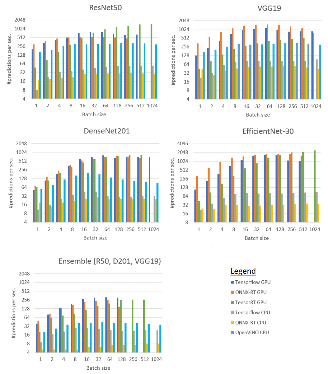
Figure A.1: Machine A.

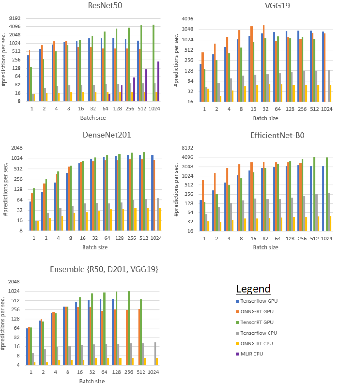
Figure A.2: Machine B.

Appendix B Memory consumption

Figure B.1 shows the memory consumption of the ensemble {VGG19, ResNet50, DenseNet201}. We use this ensemble due to the diversity of topology between neural networks: VGG has wider convolutions, Resnet is deeper, and Densenet contains many jumps between layers.

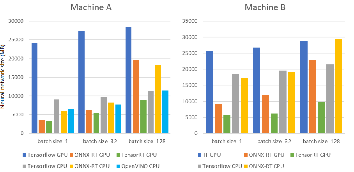
Figure B.1: Memory consumption (MB) of the ensemble with different frameworks varying the batch size.

Appendix C Power consumption

Figure C.1 presents the power consumption (Watt/sec.) of different inference frameworks (“TRT” for TensorRT, “TF” for Tensorflow, “ORT” for ONNX-RT) with {1,32,128} batch size. The model running is the ensemble {VGG19, Resnet50, DenseNet201}.

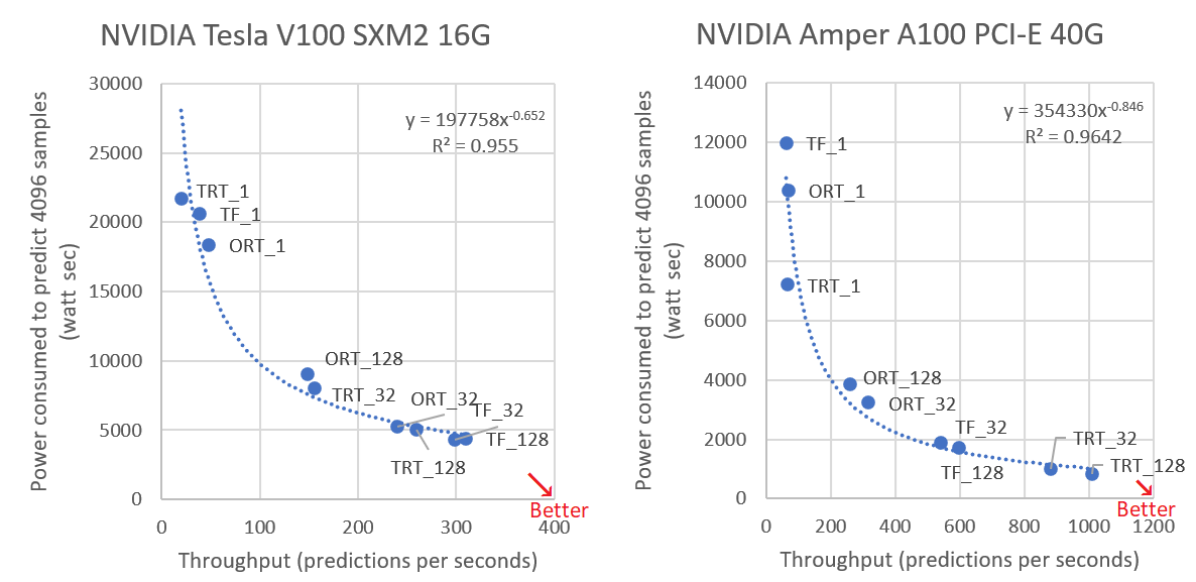
Figure C.1: Plot of the throughput and power consumption

We use the below command to measure power draw:

nvidia-smi -i ${GPUID} --format=csv --query-gpu=power.draw --loop-ms=3000

with $GPUID the corresponding GPU identifier hosting the neural network.

References

- [1] P. Davoodi, C. Gwon, G. Lai, and T. Morris, “Tensorrt inference with tensorflow,” 2019, GPU Technology Conference.
- [2] D. D. Sarah Bird, “ONNX,” in Workshop NIPS2017, 2017.
- [3] Y. Ge and M. Jones, “Inference with intel,” 2018, aI DevCon 2018.
- [4] C. Leary and T. Wang, “Xla: Tensorflow, compiled!” in Tensorflow developer summit, 2017.
- [5] C. Lattner, M. Amini, U. Bondhugula, A. Cohen, A. Davis, J. Pienaar, R. Riddle, T. Shpeisman, N. Vasilache, and O. Zinenko, “Mlir: Scaling compiler infrastructure for domain specific computation,” in Proceedings of the 2021 IEEE/ACM International Symposium on Code Generation and Optimization, ser. CGO ’21. IEEE Press, 2021, p. 2–14. [Online]. Available: https://doi.org/10.1109/CGO51591.2021.9370308
- [6] Dominic Divakaruni, Peter Jones, Sudipta Sengupta, Liviu Calin, “Amazon elastic inference: Reduce learning inference cost,” 2018.
- [7] W. Zhang, W. Wei, L. Xu, L. Jin, and C. Li, “AI matrix: A deep learning benchmark for alibaba data centers,” CoRR, vol. abs/1909.10562, 2019. [Online]. Available: http://arxiv.org/abs/1909.10562
- [8] C. Coleman, D. Kang, D. Narayanan, L. Nardi, T. Zhao, J. Zhang, P. Bailis, K. Olukotun, C. Ré, and M. Zaharia, “Analysis of dawnbench, a time-to-accuracy machine learning performance benchmark,” SIGOPS Oper. Syst. Rev., vol. 53, no. 1, p. 14–25, jul 2019. [Online]. Available: https://doi.org/10.1145/3352020.3352024
- [9] V. J. Reddi, C. Cheng, D. Kanter, P. Mattson, G. Schmuelling, C.-J. Wu, B. Anderson, M. Breughe, M. Charlebois, W. Chou, R. Chukka, C. Coleman, S. Davis, P. Deng, G. Diamos, J. Duke, D. Fick, J. S. Gardner, I. Hubara, S. Idgunji, T. B. Jablin, J. Jiao, T. S. John, P. Kanwar, D. Lee, J. Liao, A. Lokhmotov, F. Massa, P. Meng, P. Micikevicius, C. Osborne, G. Pekhimenko, A. T. R. Rajan, D. Sequeira, A. Sirasao, F. Sun, H. Tang, M. Thomson, F. Wei, E. Wu, L. Xu, K. Yamada, B. Yu, G. Yuan, A. Zhong, P. Zhang, and Y. Zhou, “Mlperf inference benchmark,” in Proceedings of the ACM/IEEE 47th Annual International Symposium on Computer Architecture, ser. ISCA ’20. IEEE Press, 2020, p. 446–459. [Online]. Available: https://doi.org/10.1109/ISCA45697.2020.00045
- [10] Y. Liu, H. Zhang, L. Zeng, W. Wu, and C. Zhang, “Mlbench: Benchmarking machine learning services against human experts,” Proc. VLDB Endow., vol. 11, no. 10, p. 1220–1232, jun 2018. [Online]. Available: https://doi.org/10.14778/3231751.3231770
- [11] H. Guan, L. K. Mokadam, X. Shen, S.-H. Lim, and R. Patton, “Fleet: Flexible efficient ensemble training for heterogeneous deep neural networks,” in Proceedings of Machine Learning and Systems, I. Dhillon, D. Papailiopoulos, and V. Sze, Eds., vol. 2, 2020, pp. 247–261. [Online]. Available: https://proceedings.mlsys.org/paper/2020/file/ed3d2c21991e3bef5e069713af9fa6ca-Paper.pdf
- [12] P. Pochelu, S. Petiton, and B. Conche, “An efficient and flexible inference system for serving heterogeneous ensembles of deep neural networks,” in IEEE BigData 2021, Virtual, United States, Dec 2021. [Online]. Available: https://hal.archives-ouvertes.fr/hal-03494431
- [13] M. Alwani, H. Chen, M. Ferdman, and P. Milder, “Fused-layer cnn accelerators,” in 2016 49th Annual IEEE/ACM International Symposium on Microarchitecture (MICRO), 2016, pp. 1–12.
- [14] M. Guillemot, C. Heusele, R. Korichi, S. Schnebert, and L. Chen, “Breaking batch normalization for better explainability of deep neural networks through layer-wise relevance propagation,” CoRR, vol. abs/2002.11018, 2020. [Online]. Available: https://arxiv.org/abs/2002.11018
- [15] T. Chen, T. Moreau, Z. Jiang, L. Zheng, E. Yan, M. Cowan, H. Shen, L. Wang, Y. Hu, L. Ceze, C. Guestrin, and A. Krishnamurthy, “Tvm: An automated end-to-end optimizing compiler for deep learning,” in Proceedings of the 13th USENIX Conference on Operating Systems Design and Implementation, ser. OSDI’18. USA: USENIX Association, 2018, p. 579–594.
- [16] D. Crankshaw, X. Wang, G. Zhou, M. J. Franklin, J. E. Gonzalez, and I. Stoica, “Clipper: A low-latency online prediction serving system,” in 14th USENIX Symposium on Networked Systems Design and Implementation (NSDI 17). Boston, MA: USENIX Association, Mar. 2017, pp. 613–627. [Online]. Available: https://www.usenix.org/conference/nsdi17/technical-sessions/presentation/crankshaw
- [17] R. Sharma, “Amazon elastic inference: Reduce deep learning inference cost,” 2019, gPU Technology Conference.
- [18] S. Han, J. Pool, J. Tran, and W. J. Dally, “Learning both weights and connections for efficient neural networks,” in Proceedings of the 28th International Conference on Neural Information Processing Systems - Volume 1, ser. NIPS’15. Cambridge, MA, USA: MIT Press, 2015, p. 1135–1143.
- [19] D. Oktay, J. Ballé, S. Singh, and A. Shrivastava, “Scalable model compression by entropy penalized reparameterization,” in 8th International Conference on Learning Representations, ICLR 2020, Addis Ababa, Ethiopia, April 26-30, 2020. OpenReview.net, 2020. [Online]. Available: https://openreview.net/forum?id=HkgxW0EYDS
- [20] A. Polino, R. Pascanu, and D. Alistarh, “Model compression via distillation and quantization,” in International Conference on Learning Representations, 2018. [Online]. Available: https://openreview.net/forum?id=S1XolQbRW
- [21] V. Vanhoucke, A. Senior, and M. Z. Mao, “Improving the speed of neural networks on cpus,” in Deep Learning and Unsupervised Feature Learning Workshop, NIPS 2011, 2011.
- [22] M. Courbariaux, Y. Bengio, and J.-P. David, “Binaryconnect: Training deep neural networks with binary weights during propagations,” in Advances in Neural Information Processing Systems, C. Cortes, N. Lawrence, D. Lee, M. Sugiyama, and R. Garnett, Eds., vol. 28. Curran Associates, Inc., 2015. [Online]. Available: https://proceedings.neurips.cc/paper/2015/file/3e15cc11f979ed25912dff5b0669f2cd-Paper.pdf