Optimal Control for Platooning in Vehicular Networks

Abstract

As the automotive industry is developing autonomous driving systems and vehicular networks, attention to truck platooning has increased as a way to reduce costs (fuel consumption) and improve efficiency in the highway. Recent research in this area has focused mainly on the aerodynamics, network stability, and longitudinal control of platoons. However, the system aspects (e.g., platoon coordination) are still not well explored. In this paper, we formulate a platooning coordination problem and study whether trucks waiting at an initial location (station) should wait for a platoon to arrive in order to leave. Arrivals of trucks at the station and platoons by the station are modelled by independent Bernoulli distributions. Next we use the theory of Markov Decision Processes to formulate the dispatching control problem and derive the optimal policy governing the dispatching of trucks with platoons. We show that the policy that minimizes an average cost function at the station is of threshold type. Numerical results for the average cost case are presented. They are consistent with the optimal ones.

Keywords Truck platooning, Optimal control of queues.

1 Introduction

Truck platooning is the practice of virtually connecting two or more automated trucks forming convoys, where trucks follow one another closely. This practice has recently gained attention as the automotive industry develops toward autonomous driving systems and vehicular networks Adler et al. (2020). It holds great potential to make traffic more efficient and clean. In particular, allowing close-distance driving mitigates the effects of aerodynamic drag, which in turn leads to a substantial reduction in fuel consumption Zabat (1995). Platooning also optimizes highway use, reduces travel times and enhances transportation safety.

The benefits of platooning may vary due to the complex and dynamic behaviour of trucks and the resulting traffic. For instance, this potential depends on several aspects, such as the inter-vehicle gap in a platoon, the travel speed, the cost of platooning formation, and others Zabat (1995). Therefore, it is crucial to study and understand platooning under concrete mathematical models.

1.1 Related Work

Most of the research efforts so far have been concerned with studying the aerodynamic aspects of platooning Zabat (1995); Vohra et al. (2018), the cooperative longitudinal control of trucks Tsugawa et al. (2016); Hu et al. (2020); Milanes et al. (2014), and the stability of the platoons from a network perspective Wang et al. (2021); Petrillo et al. (2021). However, the system aspects (e.g., platoon coordination) are still not well explored Adler et al. (2020), especially concerning optimal control.

Previous works on platooning coordination considered the dispatching control of trucks waiting in a station/hub Zhang et al. (2017); Adler et al. (2020); A. Johansson et al. (2020). In these works, trucks arrive at the station following a random process (e.g., Poisson or Bernoulli), and the station decides whether they should wait to form platoons. If the station holds them, it may build platoons with many trucks, which reduces fuel consumption. However, forcing many trucks to wait at the station incurs high transportation delay cost. These works investigated the optimal dispatching control at the station that minimizes an average cost function.

In Zhang et al. (2017), the authors studied optimal platoon coordination at a highway junction (hub). Their model consisted of two trucks arriving at the hub with stochastic arrival times. If they arrive at the same time, they form a platoon. One truck may have to wait for the other when their arrival times differ, which incurs a waiting cost. The authors proved that it is optimal to build a platoon only when the arrival time of each truck differs by less than a threshold.

In Adler et al. (2020), the authors studied platooning coordination of multiple trucks at a station, where the arrivals are Poisson distributed. The station decides whether to hold trucks in order to build platoons. The authors compared different truck dispatching policies governing the station under energy-delay tradeoff considerations. They proved the optimality of threshold policies to control station dispatching, where the station dispatches all trucks whenever the number of waiting trucks in the station grows above the threshold. In A. Johansson et al. (2020), the authors proposed a similar model to the one in Adler et al. (2020) under the assumption that arrivals of trucks are i.i.d and their distribution is known by the station. They proved that the optimal policy is of the type "one time-step look-ahead".

1.2 Model Novelty and Main Contributions

In this paper, we study the dispatching and formation of platoons from a novel perspective. In particular, like Adler et al. (2020), A. Johansson et al. (2020) (and unlike Zhang et al. (2017)), in our model we consider a waiting station that can hold multiple trucks. However, unlike Adler et al. (2020) and A. Johansson et al. (2020), we assume that trucks arrive at the station, while platoons arrive alongside the station. Therefore, we dispatch trucks with arriving platoons, as opposed to forming platoons among waiting trucks. Our cost function is also different.

We formalize the dispatching actions at the station as an optimal control problem. We then use dynamic programming to analyze it. The main contributions of this work are as follows:

• We derive the optimal dispatching policy governing the system under finite and infinite horizon discounted cost criteria. We show that the policies are of threshold type with a finite threshold.

• We use Lippman’s Lippman (1973) results to derive the optimal policy for the average cost criterion.

• We present numerical results for the average cost case.

The paper is organized as follows. In Section 2, we formulate the dispatching trucks to arriving platoons problem. We also present the Markov Decision Problem. We characterize the optimal control policy for the discounted cost (with finite and infinite horizons) in Section 3. In Section 4, we derive the optimal policy for the average cost problem. We present some numerical results for the average cost problem in Section 5. Our conclusion and suggestions for future work are presented in Section 6.

2 Model and Control Problem Formulation

We consider the platooning system shown in Figure 1.

Figure 1: System model.

Define the station as a location where trucks arrive and can wait to join platoons. Platoons arrive alongside the station. The station decides how trucks are dispatched from the station. We assume that only one truck at a time can be dispatched.

The system operates in discrete time. Truck arrivals are Bernoulli with parameter $p$. Trucks join the same queue upon arrival. Platoon arrivals are Bernoulli with parameter $q$. In order to avoid trivialities, we assume that $0<p<1$ and $0<q<1$.

We assume truck and platoon arrivals are a sequence of ordered events in one time slot. A truck arrival (if any) always takes place earlier than a platoon arrival (if any). This assumption guarantees that if the station is empty and a truck arrives, it can join a platoon if any arrives.

2.1 The Markovian Decision problem

Let $x_{n}$ denote the number of trucks waiting at the station at slot $n$, $n\in\{1,2,\dots\}$. $x_{n}$ is the state of the system and $X=\{0,1,2,\dots\}$ is the state space of the system.

Define the events as the combinations of arrivals (of a truck or a platoon) that may occur during a time slot. Each event has a given probability and a state operator (mapping $X$ into $X$). Transitions among the states are described in Table 1.

Events	State Operators	Probabilities
No arrivals.	$Z(x)=x.$	$(1-p)(1-q)$
A platoon arrives and no truck arrives.	$P(x)=x.$	$(1-p)q$
A truck arrives and no platoon arrives.	$V(x)=x+1.$	$p(1-q)$
A platoon and a truck arrive.	$B(x)=x+1.$	$pq$

Table 1: Events, State Operators, and Probabilities.

Define the action space $\mathcal{A}=\{H,D\}$, where the action operator $H$ represents the action of holding a truck at the station, and $D$ denotes the dispatching action. We have:

$$H(x) =x,\operatorname{\textit{ \leavevmode\nobreak\ \leavevmode\nobreak\ \leavevmode\nobreak\ \leavevmode\nobreak\ \leavevmode\nobreak\ dom }}H=X.$$

$$D(x) =x-1,\operatorname{\textit{ dom }}D=\{x\in X:x\geq 1\}.$$

$\mathcal{A}(x_{n})$ represents the available actions for a given state $x_{n}$ at time slot $n$.

Dispatching trucks with platoons reduces energy (fuel) consumption. Holding trucks at the station (when waiting for platoons) incurs transportation delay costs. Trucks dispatched without platoons pay the entire transportation cost.

We assume all arriving platoons provide the same energy reduction. It simplifies the model as the cost of dispatching a truck by platooning (or not) becomes deterministic. We introduce a real-valued constant $\kappa$ representing the cost of dispatching a truck without a platoon.

We formalize these assumptions mathematically with $c(x_{n},a_{n})$, the instantaneous cost as a function of the system state $x_{n}$ when taking the action $a_{n}$ at time slot $n$. More specifically, satisfies:

$$c(x_{n},a_{n})=\begin{cases}x_{n}&\text{if }a_{n}=H.\\ x_{n}-1&\text{if}\text{ a platoon arrives and }a_{n}=D.\\ x_{n}-1+\kappa&\text{if}\text{ no platoon arrives and }a_{n}=D.\end{cases}$$ (1)

We complete the specification of our Markov Decision Problem (MDP) by defining the transition probability function as follows:

$$P(x_{n+1}|x_{n}=x,a_{n})=\begin{cases}(1-p)(1-q)&\text{ if }x_{n+1}=Z(x),\hskip 14.22636pta_{n}=H.\\ (1-p)(1-q)&\text{ if }x_{n+1}=x-1,\hskip 11.9501pta_{n}=D.\\ (1-p)q&\text{ if }x_{n+1}=P(x),\hskip 13.942pta_{n}=H.\\ (1-p)q&\text{ if }x_{n+1}=x-1,\hskip 12.23447pta_{n}=D.\\ p(1-q)&\text{ if }x_{n+1}=V(x),\hskip 13.942pta_{n}=H.\\ p(1-q)&\text{ if }x_{n+1}=x,\hskip 31.2982pta_{n}=D.\\ pq&\text{ if }x_{n+1}=B(x),\hskip 13.942pta_{n}=H.\\ pq&\text{ if }x_{n+1}=x,\hskip 31.2982pta_{n}=D.\end{cases}$$ (2)

Our goal is to choose the control actions to minimize the expected finite horizon discounted cost, as

$$\mathbb{E}\sum_{n=1}^{N}\beta^{n}c(x_{n},a_{n}),$$ (3)

where $\beta$ is a discount factor $0<\beta<1$, and $N$ is the time horizon.

Since $c(x_{n},a_{n})$ grows linearly $\forall x\in X$ and $N$ is finite, it is well known that there exists an optimal stationary (time-independent) policy that minimizes the cost (3) and is the unique solution for the MDP.

Define $J^{\beta}_{N}(x)$ as the minimum expected discounted cost for (3) with $N$ steps to go and initial state $x_{0}=x$. $J^{\beta}_{N}(x)$ satisfies:

$$J^{\beta}_{N}(x)=\min\limits_{a\in\mathcal{A}(x)}\{c(x,a)+\beta[(1-p)(1-q){J^{\beta}_{N-1}(}Z(x{))}+(1-p)q{J^{\beta}_{N-1}(}P(x){)}\,+$$

$$\hskip 201.7868ptp(1-q){J^{\beta}_{N-1}(}V(x){)}+pq{J^{\beta}_{N-1}(}B(x){)}]\},$$ (4)

where the initial condition is $J^{\beta}_{1}(x)=\min\{c(x,a)|\leavevmode\nobreak\ a\in\mathcal{A}(x)\}$.

From the Dynamic Programming (DP) equation (4), we immediately see that with $n+1$ steps to go and initial state $x_{0}=x$, the optimal action $a$ is given by the difference $J_{n+1}^{\beta}(H(x))-J_{n+1}^{\beta}(D(x))$, as:

$$a=\left\{\begin{array}[]{@{}lr@{}}\hbox{\multirowsetup H, \leavevmode\nobreak\ \leavevmode\nobreak\ if}&(1-p)(1-q)[{J^{\beta}_{n}}(x)-{J^{\beta}_{n}}(x-1)]+(1-p)q[{J^{\beta}_{n}}({x})-{J^{\beta}_{n}}({x-1})]\nobreak\leavevmode\nobreak\leavevmode\\ &+\,p(1-q)[{J^{\beta}_{n}}(x+1)-{J^{\beta}_{n}}(x)]+pq[{J^{\beta}_{n}}({x+1})-{J^{\beta}_{n}}({x})]\leq\dfrac{-1+\kappa}{\beta}.\vspace{.cm}\\ \\ \hbox{\multirowsetup D, \leavevmode\nobreak\ \leavevmode\nobreak\ if}&(1-p)(1-q)[{J^{\beta}_{n}}(x)-{J^{\beta}_{n}}(x-1)]+(1-p)q[{J^{\beta}_{n}}({x})-{J^{\beta}_{n}}({x-1})]\nobreak\leavevmode\nobreak\leavevmode\\ &+\,p(1-q)[{J^{\beta}_{n}}(x+1)-{J^{\beta}_{n}}(x)]+pq[{J^{\beta}_{n}}({x+1})-{J^{\beta}_{n}}({x})]>\dfrac{-1+\kappa}{\beta}.\\ \end{array}\color[rgb]{1,1,1}\right\}$$ (10)

We will use (10) to characterize the optimal policy for (4) in the next section.

3 Characterization of the Optimal Policy

In this section, we first prove some properties of the optimal cost function; we then use them to characterize the optimal policy as a threshold policy.

The following Lemma (which we can show using Equations (1) and (4)) simplifies the search for an optimal policy, since we can disregard the holding actions with probabilities $pq$ and $(1-p)q$ in Equation (2).

Lemma 3.1.

Dispatching a truck with an arriving platoon is always optimal.

Proof.

We use induction on $n$ to prove that when a platoon arrives

$$J^{\beta}_{n}(D(x))\leq J^{\beta}_{n}(H(x)),\leavevmode\nobreak\ \forall x\in\text{dom}\leavevmode\nobreak\ D.$$ (11)

Base case ($n=1$). This proof is immediate since $J^{\beta}_{1}(x)$ is the instantaneous cost (1) and when the system state is $x_{n}\geq 1$ and a platoon arrives, $c(x_{n},D)<c(x_{n},H)$ for all $x\in\text{dom}\leavevmode\nobreak\ D$.

Inductive step (from $n=N$ to $n=N+1$). Assume that Inequality (11) is valid with $n=N$, for all $x\in\text{dom}\leavevmode\nobreak\ D$. We will prove the same is true for all $x$ and $n=N+1$, i.e.,

$$J^{\beta}_{N+1}(D(x))\leq J^{\beta}_{N+1}(H(x)).$$ (12)

We replace (4) in (12) and apply the operators $H$ and $D$ to obtain

$$x -1+\beta[(1-p)(1-q){J^{\beta}_{N}(}x-1{)}+(1-p)q{J^{\beta}_{N}(}x-1{)}+p(1-q){J^{\beta}_{N}}(x)+pq{J^{\beta}_{N}(}x{)}]$$

$$\leq x+\beta[(1-p)(1-q){J^{\beta}_{N}}(x)+(1-p)q{J^{\beta}_{N}(}x{)}+p(1-q){J^{\beta}_{N}(}x+1{)}+pq{J^{\beta}_{N}(}x+1{)}].$$

We now cancel identical terms and rearrange them to derive

$$-1+\beta[(1-p)(1-q)[{J^{\beta}_{N}(}x-1{)}-{J^{\beta}_{N}}(x)]+(1-p)q[{J^{\beta}_{N}(}x-1{)}-{J^{\beta}_{N}(}x{)}]\,+$$

$$\hskip 133.72786ptp(1-q)[{J^{\beta}_{N}}(x)-{J^{\beta}_{N}}(x+1)]+pq[{J^{\beta}_{N}(}x{)}-{J^{\beta}_{N}(}x+1{)}]]\leq\,0.$$ (13)

From (13), all we have to show is that $J^{\beta}_{N+1}(x)$ is monotone increasing for all $x$. However, since $J^{\beta}_{N}(x)$ is convex and $c(x_{n},a_{n})$ grows linearly $\forall x\in X$ (see Theorem 1), monotonicity is sufficed. Therefore, Inequality (11) is valid for all $n\in N$ and $x\in\text{dom}\leavevmode\nobreak\ D$. ∎

In Figure 2, we show the transition probabilities.

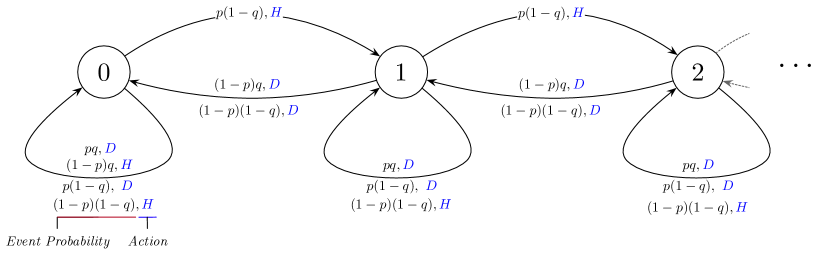
Figure 2: Transition probabilities using the result of Lemma 3.1.

Theorem 1.

For each $n\geq 1$, the function $J^{\beta}_{n}$ is convex. Moreover, the difference $J_{n+1}^{\beta}(H(x))-J_{n+1}^{\beta}(D(x))$ is monotone increasing.

Proof.

We first prove the convexity of $J^{\beta}_{n}$. We use induction on $n$ to prove that for all $x$

$$J^{\beta}_{n}(x+1)+J^{\beta}_{n}(x-1)\geq 2J^{\beta}_{n}(x).$$ (14)

Base case ($n=1$). This is immediate if we recall that $J^{\beta}_{1}(x)=c(x,a)$, which is a linear function in $x$, for all $a$.

Inductive step (from $n=N$ to $n=N+1$). Assume that Inequality (14) is valid with $n=N$, for all $x$. We will prove the same is true for $n=N+1$, i.e.,

$$J^{\beta}_{N+1}(x+1)+J^{\beta}_{N+1}(x-1)\geq 2J^{\beta}_{N+1}(x),$$ (15)

for all $x$ and $a\in\{H,D\}$.

Remark: Using (15), we can see that there are eight possible combinations of actions as $a\in\{H,D\}$. However, from (10), it follows that we need to prove that (15) holds only for four of the cases, since once $D$ is optimal for $x$ (i.e., $x>m$), $D$ is optimal for all $x^{\prime}>x$.

Case 1: Holding action for $x-1$, $x$, and $x+1$.
Applying the holding action to (4), the following identity holds

$$J^{\beta}_{N+1}(x) =x+\beta((1-p)(1-q)J^{\beta}_{N}(x)+p(1-q)J^{\beta}_{N}(x+1)\,+(1-p)qJ^{\beta}_{N}({x})+pqJ^{\beta}_{N}({x+1})).$$ (16)

We apply Identity (16) to $x-1$ and $x+1$ and we derive

$$J^{\beta}_{N+1}(x+1) =x+1+\beta((1-p)(1-q)J^{\beta}_{N}(x+1)+p(1-q)J^{\beta}_{N}(x+2)+(1-p)qJ^{\beta}_{N}({x+1})\,+$$

$$\hskip 327.20668ptpqJ^{\beta}_{N}({x+2})).$$ (17)

$$J^{\beta}_{N+1}(x-1) =x-1+\beta((1-p)(1-q)J^{\beta}_{N}(x-1)+p(1-q)J^{\beta}_{N}(x)\,+(1-p)qJ^{\beta}_{N}({x-1})+pqJ^{\beta}_{N}({x})).$$ (18)

Substituting Identities (16), (3), and (18) into Inequality (15) we obtain

$$x+1+\beta((1-p)(1-q)J^{\beta}_{N}(x+1)+p(1-q)J^{\beta}_{N}(x+2)+(1-p)qJ^{\beta}_{N}({x+1})+pqJ^{\beta}_{N}({x+2}))$$

$$+x-1+\beta((1-p)(1-q)J^{\beta}_{N}(x-1)+p(1-q)J^{\beta}_{N}(x)+(1-p)qJ^{\beta}_{N}({x-1})+pqJ^{\beta}_{N}({x}))$$

$$\geq 2(x+\beta((1-p)(1-q)J^{\beta}_{N}(x)+p(1-q)J^{\beta}_{N}(x+1)+(1-p)qJ^{\beta}_{N}({x})+pqJ^{\beta}_{N}({x+1}))).$$ (19)

Rearranging Inequality (3) as indicated, all we need to prove is

$$(1-p)(1-q)(J^{\beta}_{N}(x+1)+J^{\beta}_{N}(x-1)-2J^{\beta}_{N}(x))+p(1-q)(J^{\beta}_{N}(x+2)+J^{\beta}_{N}(x)-2J^{\beta}_{N}(x+1))+$$

$$(1-p)q(J^{\beta}_{N}({x+1})+J^{\beta}_{N}({x-1})-2J^{\beta}_{N}({x}))\,+pq(J^{\beta}_{N}({x+2})+J^{\beta}_{N}({x})-2J^{\beta}_{N}({x+1}))\geq 0.$$

However, this is obvious using the convexity of $J^{\beta}_{N}$, which is true by the inductive hypothesis.

Case 2: Dispatching action for $x-1$, $x$, and $x+1$.
Applying the dispatching action to (4), the following identity holds

$$J^{\beta}_{N+1}(x) =x-1+\kappa+\beta((1-p)(1-q)J^{\beta}_{N}(x-1)+p(1-q)J^{\beta}_{N}(x)\,+(1-p)qJ^{\beta}_{N}({x-1})+pqJ^{\beta}_{N}({x})).$$ (20)

If we also apply Identity (20) to $x-1$ and $x+1$ and derive

$$J^{\beta}_{N+1}(x+1) =x+\kappa+\beta((1-p)(1-q)J^{\beta}_{N}(x)+p(1-q)J^{\beta}_{N}(x+1)\,+(1-p)qJ^{\beta}_{N}({x})+pqJ^{\beta}_{N}({x+1})).$$ (21)

$$J^{\beta}_{N+1}(x-1) =x-2+\kappa+\beta((1-p)(1-q)J^{\beta}_{N}(x-2)+p(1-q)J^{\beta}_{N}(x-1)\,+$$

$$\hskip 236.15796pt(1-p)qJ^{\beta}_{N}({x-2})+pqJ^{\beta}_{N}({x-1})).$$ (22)

Substituting Identities (20), (3), and (21) into Inequality (15) we obtain

$$x+\kappa+\beta((1-p)(1-q)J^{\beta}_{N}(x)+p(1-q)J^{\beta}_{N}(x+1)\,+(1-p)qJ^{\beta}_{N}({x})+pqJ^{\beta}_{N}({x+1}))\,+$$

$$x-2+\kappa+\beta((1-p)(1-q)J^{\beta}_{N}(x-2)+p(1-q)J^{\beta}_{N}(x-1)\,+(1-p)qJ^{\beta}_{N}({x-2})+$$

$$pqJ^{\beta}_{N}({x-1}))+\geq 2(x-1+\kappa+\beta((1-p)(1-q)J^{\beta}_{N}(x-1)+p(1-q)J^{\beta}_{N}(x)\,+$$

$$\hskip 256.0748pt(1-p)qJ^{\beta}_{N}({x-1})+pqJ^{\beta}_{N}({x}))).$$ (23)

Rearranging Inequality (23) as indicated, all we need to prove is

$$(1-p)(1-q)(J^{\beta}_{N}(x)+J^{\beta}_{N}(x-2)-2J^{\beta}_{N}(x-1))+p(1-q)(J^{\beta}_{N}(x+1)+J^{\beta}_{N}(x-1)-2J^{\beta}_{N}(x))$$

$$+(1-p)q(J^{\beta}_{N}({x})+J^{\beta}_{N}({x-2})-2J^{\beta}_{N}({x-1}))\,+pq(J^{\beta}_{N}({x+1})+J^{\beta}_{N}({x-1})-2J^{\beta}_{N}({x}))\geq 0,$$

which is true by the inductive hypothesis.

Case 3: Dispatching action for $x$ and $x+1$, and holding action for $x-1$.
Substituting Identities (18), (20), and (21) into Inequality (15) we obtain

$$x+\kappa+\beta((1-p)(1-q)J^{\beta}_{N}(x)+p(1-q)J^{\beta}_{N}(x+1)\,+(1-p)qJ^{\beta}_{N}({x})+pqJ^{\beta}_{N}({x+1}))\,+$$

$$x-1+\beta((1-p)(1-q)J^{\beta}_{N}(x-1)+p(1-q)J^{\beta}_{N}(x)+(1-p)qJ^{\beta}_{N}({x-1})+pqJ^{\beta}_{N}({x}))\geq$$

$$2(x-1+\kappa+\beta((1-p)(1-q)J^{\beta}_{N}(x-1)+p(1-q)J^{\beta}_{N}(x)\,+(1-p)qJ^{\beta}_{N}({x-1})+pqJ^{\beta}_{N}({x}))).$$

Since (18) is identical to (20), we cancel equivalent terms to derive

$$x+\kappa+\beta((1-p)(1-q)J^{\beta}_{N}(x)+p(1-q)J^{\beta}_{N}(x+1)\,+(1-p)qJ^{\beta}_{N}({x})+pqJ^{\beta}_{N}({x+1}))\geq x-1$$

$${+\,\kappa+\beta((1-p)(1-q)J^{\beta}_{N}(x-1)+p(1-q)J^{\beta}_{N}(x)\,+(1-p)qJ^{\beta}_{N}({x-1})+pqJ^{\beta}_{N}({x}))}.$$ (24)

Rearranging Inequality (24) as indicated, all we need to prove is

$$(1-p)(1-q)(J^{\beta}_{N}(x)-J^{\beta}_{N}(x-1))+p(1-q)(J^{\beta}_{N}(x+1)-J^{\beta}_{N}(x))\,+$$

$$\hskip 48.36958pt(1-p)q(J^{\beta}_{N}({x})-J^{\beta}_{N}({x-1}))+pq(J^{\beta}_{N}({x+1})-J^{\beta}_{N}({x})))\geq\frac{\kappa-1}{\beta}.$$ (25)

Since (25) is identical to (10), the left side of (25) is greater than its right side whenever the dispatching action is taken. Thus, Inequality (25) holds.

Case 4: Dispatching action for $x+1$, and holding action for $x-1$ and $x$.
Substituting Identities (16), (18), and (21) into Inequality (15) we obtain

$$x+\kappa+\beta((1-p)(1-q)J^{\beta}_{N}(x)+p(1-q)J^{\beta}_{N}(x+1)\,+(1-p)qJ^{\beta}_{N}({x})+pqJ^{\beta}_{N}({x+1}))\,+$$

$$x-1+\beta((1-p)(1-q)J^{\beta}_{N}(x-1)+p(1-q)J^{\beta}_{N}(x)+(1-p)qJ^{\beta}_{N}({x-1})+pqJ^{\beta}_{N}({x}))\geq$$

$$2(x+\beta((1-p)(1-q)J^{\beta}_{N}(x)+p(1-q)J^{\beta}_{N}(x+1)+(1-p)qJ^{\beta}_{N}({x})+pqJ^{\beta}_{N}({x+1}))).$$ (26)

Since (16) is identical to (21) (except for $\kappa$), we cancel equivalent terms to derive

$$\kappa+x-1+\beta((1-p)(1-q)J^{\beta}_{N}(x-1)+p(1-q)J^{\beta}_{N}(x)+(1-p)qJ^{\beta}_{N}({x-1})+pqJ^{\beta}_{N}({x}))$$

$$\geq x+\beta((1-p)(1-q)J^{\beta}_{N}(x)+p(1-q)J^{\beta}_{N}(x+1)+(1-p)qJ^{\beta}_{N}({x})+pqJ^{\beta}_{N}({x+1})).$$ (27)

Rearranging Inequality (27) as indicated, all we need to prove is

$$(1-p)(1-q)(J^{\beta}_{N}(x-1)-J^{\beta}_{N}(x))+p(1-q)(J^{\beta}_{N}(x)-J^{\beta}_{N}(x+1))\,+$$

$$\hskip 49.79231pt(1-p)q(J^{\beta}_{N}({x-1})-J^{\beta}_{N}({x}))+pq(J^{\beta}_{N}({x})-J^{\beta}_{N}({x-1})))\geq\frac{1-\kappa}{\beta}.$$ (28)

Multiplying (28) by $-1$, we obtain (10) when the holding action is chosen. Since both equations in (28) take the holding action, (28) holds by (10).

Monotonicity.

To prove that the difference $J_{N}^{\beta}(H(x))-J_{N}^{\beta}(D(x))$ is monotone increasing, we have to show that

$$\text{i.e.,\leavevmode\nobreak\ \leavevmode\nobreak\ \leavevmode\nobreak\ \leavevmode\nobreak\ }J_{N}^{\beta}(H(x))-J_{N}^{\beta}(D(x))\geq J_{N}^{\beta}(H(x-1))-J_{N}^{\beta}(D(x-1)),\leavevmode\nobreak\ \leavevmode\nobreak\ \leavevmode\nobreak\ \leavevmode\nobreak\ \leavevmode\nobreak\ \leavevmode\nobreak\ \leavevmode\nobreak\ \leavevmode\nobreak\ \forall x\geq 1.$$ (29)

Using Inequality (10), we have to show that for every $x>m$, the following inequality holds

$$\dfrac{-\kappa+1}{\beta}+(1-p)(1-q)({J^{\beta}_{n}}(x)-{J^{\beta}_{n}}(x-1))+(1-p)q({J^{\beta}_{n}}({x})-{J^{\beta}_{n}}({x-1}))\,+$$

$$\hskip 128.0374ptp(1-q)({J^{\beta}_{n}}(x+1)-{J^{\beta}_{n}}(x))+pq({J^{\beta}_{n}}({x+1})-{J^{\beta}_{n}}({x}))\geq$$

$$\dfrac{-\kappa+1}{\beta}+(1-p)(1-q)({J^{\beta}_{n}}(m)-{J^{\beta}_{n}}(m-1))+(1-p)q({J^{\beta}_{n}}({m})-{J^{\beta}_{n}}({m-1}))\,+$$

$$\hskip 113.81102ptp(1-q)({J^{\beta}_{n}}(m+1)-{J^{\beta}_{n}}(m))+pq({J^{\beta}_{n}}({m+1})-{J^{\beta}_{n}}({m}))>0.$$ (30)

We cancel identical terms in Inequality (30) and rearrange it to derive

$$(1-p)(1-q)({J^{\beta}_{n}}(x)-{J^{\beta}_{n}}(x-1)-(J^{\beta}_{n}(m)-J^{\beta}_{n}(m-1)))\,+$$

$$\hskip 56.9055ptp(1-q)({J^{\beta}_{n}}(x+1)-{J^{\beta}_{n}}(x)-({J^{\beta}_{n}}(m+1)-{J^{\beta}_{n}}(m)))\,+$$

$$\hskip 85.35826pt(1-p)q({J^{\beta}_{n}}({x})-{J^{\beta}_{n}}({x-1})-({J^{\beta}_{n}}({m})-{J^{\beta}_{n}}({m-1})))\,+$$

$$\hskip 130.88284ptpq({J^{\beta}_{n}}({x+1})-{J^{\beta}_{n}}({x})-({J^{\beta}_{n}}({m+1})-{J^{\beta}_{n}}))>0.$$ (31)

Since $J^{\beta}_{N}$ is convex and finite for all $x\in X$, Inequality (31) holds and so (29). ∎

From Equation 10 and this theorem, $\kappa\leq 1$ is a trivial case for which dispatching a truck (action $D$) is always optimal.

Denote by $\pi_{m}$ a threshold policy with threshold $m$. Under policy $\pi_{m}$, the station dispatches a truck if and only if $x>m$ (with or without a platoon arrival).

Theorem 2.

The optimal policy for the finite horizon discounted cost problem is of threshold type with a finite threshold.

Consider next the infinite horizon, discounted cost. This cost is defined as

$$J^{\beta}(x)=\lim_{n\rightarrow\infty}J_{n}^{\beta}(x).$$

Since $c(x_{n},a_{n})$ grows linearly $\forall x\in X$, it is also well known (e.g., see Lippman (1973)) that an optimal stationary policy exists and is the unique solution to the functional equation of dynamic programming.

Theorem 3.

The optimal policy for the infinite horizon discounted cost problem is of threshold type.

Note that the theorem does not imply that the threshold is finite; this would depend on (how small) the value of the discount factor $\beta$ is.

We extend Theorem 3 to the average cost case in the next section.

4 The Average Cost problem

In the average cost sense, we want to choose the dispatching actions so as to minimize the (long-run) average cost

$$\limsup\limits_{N\rightarrow\infty}\dfrac{1}{N}\mathop{\mathbb{E}}\sum_{n=1}^{N}c(x_{n},a_{n}).$$ (32)

Let $J_{\pi}^{\beta}(x)$, $J_{\pi}$ denote the infinite horizon, discounted cost and long-run average cost incurred by a policy $\pi$. It was shown in Lippman (1973) that, if a policy $\pi$ results in a Markov chain with a single positive recurrent class, both costs are well defined and

$$\lim\limits_{\beta\rightarrow 1^{-}}(1-\beta)J_{\pi}^{\beta}(x)=J_{\pi},$$ (33)

for any $x\in X$.

Define $J_{\pi_{m}}$ as the average cost of using the threshold policy $\pi_{m}$. We follow an approach similar to the one in Lin and Kumar (1984), to prove the optimality of $\pi_{m}$ for the average cost criterion.

The following lemma shows that this cost is well-defined and finite.

Lemma 4.1.

For any finite threshold $m\geq 0$, the average cost of the policy $\pi_{m}$ is finite and given by:

$$J_{\pi_{m}}=\begin{cases}p(1-q)\kappa.\leavevmode\nobreak\ \leavevmode\nobreak\ \leavevmode\nobreak\ \leavevmode\nobreak\ \text{ if }m=0.\\ \\ \dfrac{p(1-q)}{A+1}+\dfrac{A(p(1-q)(1+\kappa)+(1-p)(1-q)+pq)}{A+1},\leavevmode\nobreak\ \leavevmode\nobreak\ \leavevmode\nobreak\ \leavevmode\nobreak\ \text{ if }m=1.\\ \\ \dfrac{m^{2}+m-2(\kappa+1)(p-1)p}{2(m+1)},\leavevmode\nobreak\ \leavevmode\nobreak\ \text{ if }m\geq 2\text{ and }p=q.\\ \\ \dfrac{p(1-q)(1-A)}{1-A^{m+1}}+\dfrac{A^{2}(-p+q)+A(1+p-q)+A^{m}(-m-p+q)}{(1-A)(1-A^{m+1})}+\vspace{0.2cm}\\ \dfrac{A^{m+1}(m+p-q-1)}{(1-A)(1-A^{m+1})}+(m-q+pq(1-\kappa)+p\kappa)\Big{(}\dfrac{A^{m}-A^{m+1}}{1-A^{m+1}}\Big{)},\text{ if }m\geq 2\text{ and }p\neq q.\end{cases}$$ (34)

where

$$A=\frac{p(1-q)}{(1-p)q}.$$ (35)

Proof.

Let $f(x)$ be the steady-state probability of the state $x\in X$ when $\pi_{m}$ is applied. ($\pi_{m}$ has a unique steady-state distribution since, under $\pi_{m}$, (i) the queue will never drift to the infinity and (ii) the state $x=0$ can be reached from every state in $X$.) $f(x)$ is defined as:

$$f(x) =(1-p)(1-q)f(\pi_{m}(Z(x)))+(1-p)qf(\pi_{m}(P(x)))+p(1-q)f(\pi_{m}(V(x)))+pqf(\pi_{m}(B(x))).$$ (36)

The state transition diagram using policy $\pi_{m}$ and the definition (36) is shown in Figure 3.

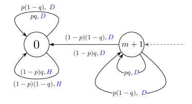
(a) For $m=0$.

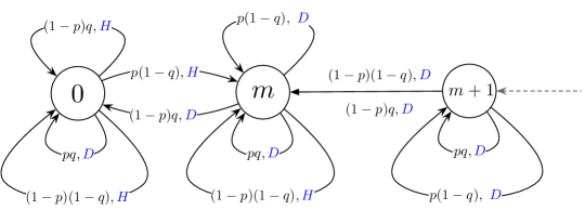
(b) For $m=1$.

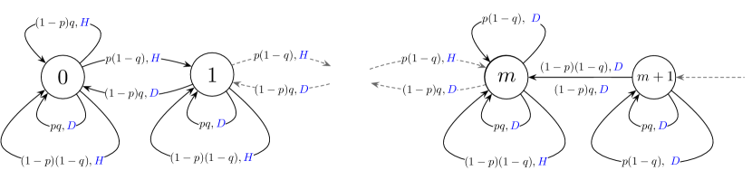
(c) For $m\geq 2$.

Figure 3: State transition diagram resulting from a threshold policy with threshold $m$.

Using the definition of $\pi_{m}$ and (36), we derive for $m\geq 2$

$$\text{if \leavevmode\nobreak\ }x=0,\hskip 46.94687pt f(0)=((1-p)q+pq+(1-p)(1-q))f(0)+((1-p)q)f(1).$$ (37)

$$\text{if \leavevmode\nobreak\ }x\in[1,m-1],\hskip 11.9501pt f(x)=(p(1-q))f(x-1)+((1-p)(1-q)+pq)f(x)$$

$$\hskip 120.92421pt+((1-p)q+(1-p)(1-q))f(x+1).$$ (38)

$$\text{if \leavevmode\nobreak\ }x=m,\hskip 42.9635pt f(m)=(p(1-q))f(m-1)+((1-p)(1-q)+pq+p(1-q))f(m)$$

$$\hskip 126.61467pt+((1-p)q+(1-p)(1-q))f(m+1).$$ (39)

$$\text{if \leavevmode\nobreak\ }x>m,\hskip 43.2483pt f(x)=(p(1-q)+pq)f(x)+((1-p)q+(1-p)(1-q))f(x+1).$$ (40)

It is more convenient to rewrite (37), (38), and (39) as:

$$f(0)=(1-p(1-q))f(0)+((1-p)q)f(1).$$ (41)

$$f(x)=(p(1-q))f(x-1)+(1-p(1-q)-(1-p)q)f(x)+((1-p)q)f(x+1).$$ (42)

$$f(m)=(p(1-q))f(m-1)+(1-q+pq)f(m)+(1-p)f(m+1).$$ (43)

Using (41), we deduce $f(1)$ as:

$$f(1) =\frac{-(1-p(1-q))f(0)+f(0)}{(1-p)q}$$

$$=\frac{-f(0)+(p(1-q))f(0)+f(0)}{(1-p)q}$$

$$=\bigg{(}\frac{p(1-q)}{(1-p)q}\bigg{)}f(0).$$ (44)

From (42) and (44), we deduce $f(2)$:

$$f(1) =(p(1-q))f(0)+(1-p(1-q)-(1-p)q)f(1)+((1-p)q)f(2).$$

$$f(2) =\frac{f(1)-(p(1-q))f(0)+(-1+p(1-q)+(1-p)q)f(1)}{(1-p)q}.$$ (45)

We cancel the terms $-f(1)+f(1)$ to derive

$$f(2) =\frac{f(1)-f(1)-(p(1-q))f(0)+(p(1-q)+(1-p)q)f(1)}{(1-p)q}.$$

$$=-\bigg{(}\frac{p(1-q)}{(1-p)q}\bigg{)}f(0)+\bigg{(}\frac{p(1-q)+(1-p)q}{(1-p)q}\bigg{)}f(1).$$

$$=-\bigg{(}\frac{p(1-q)}{(1-p)q}\bigg{)}f(0)+\bigg{(}\frac{p(1-q)}{(1-p)q}+{1}\bigg{)}f(1)$$

Replacing $f(1)$ by (44), we obtain:

$$f(2) =-\bigg{(}\frac{p(1-q)}{(1-p)q}\bigg{)}f(0)+\bigg{(}\frac{p(1-q)}{(1-p)q}+{1}\bigg{)}\bigg{(}\frac{p(1-q)}{(1-p)q}\bigg{)}f(0).$$

$$=\bigg{(}\frac{p(1-q)}{(1-p)q}\bigg{)}\bigg{(}\frac{p(1-q)}{(1-p)q}\bigg{)}f(0).$$ (46)

Define $A$ as

$$A =\frac{p(1-q)}{(1-p)q}.$$ (47)

We replace $A$ in (46) (as it will repeat quite often)

$$f(2) =A^{2}f(0).$$ (48)

By induction (see Lemma 4.2), we rewrite (42) for all $x\in[1,m]$ as:

$$f(x) =A^{x}f(0).$$ (49)

We now derive the result for $x>m$. We can simplify (40) as

$$f(x) =(p(1-q)+pq)f(x)+((1-p)q+(1-p)(1-q))f(x+1).$$

$$=(p-pq+pq)f(x)+(q-pq+1-p-q+pq)f(x+1).$$

$$=pf(x)+(1-p)f(x+1).$$

$$(1-p)f(x) =(1-p)f(x+1).$$

$$f(x) =f(x+1).$$ (50)

The result in (50) holds for all $x>m$. We now derive $f(m)$ where $x=m$ using (43), we also solve (50).

$$f(m) =(p(1-q))f(m-1)+(1-q+pq)f(m)+(1-p)f(m+1).$$

$$f(m+1) =\frac{-(p(1-q))f(m-1)+((1-p)q)f(m)}{1-p}.$$

$$=-\frac{p(1-q)}{1-p}f(m-1)+qf(m).$$

$$=-\frac{p(1-q)}{1-p}A^{m-1}f(0)+q\bigg{(}\frac{p(1-q)}{(1-p)q}\bigg{)}A^{m-1}f(0).$$

$$=-\frac{p(1-q)}{1-p}A^{m-1}f(0)+\frac{p(1-q)}{(1-p)}A^{m-1}f(0).$$

$$=0$$ (51)

The result in (51) holds for all $x>m$. We collect all the results as follows

if $$1\leq x\leq m,\hskip 33.85884ptf(x)=A^{x}f(0).$$ (52)

if $$x>m,\hskip 52.06859ptf(x)=0.$$ (53)

We obtain $f(0)$ from the condition that the sum of the probabilities is unity.

$$f(0)=\begin{cases}\dfrac{A-1}{A^{m+1}-1}\leavevmode\nobreak\ \leavevmode\nobreak\ \leavevmode\nobreak\ \leavevmode\nobreak\ \text{if}\leavevmode\nobreak\ \leavevmode\nobreak\ p\neq q.\\ \\ \dfrac{1}{m+1}.\leavevmode\nobreak\ \leavevmode\nobreak\ \leavevmode\nobreak\ \leavevmode\nobreak\ \text{if}\leavevmode\nobreak\ \leavevmode\nobreak\ p=q.\end{cases}$$ (54)

Let the $J_{\pi_{m}}$ be the cost of using policy $\pi_{m}$ to govern the platooning system.

$$J_{\pi_{m}}=\sum_{x}c(x,a)f(x).$$ (55)

Since $c(x,a)\in\{x,x-1,x-1+\kappa\}$ for all $x\in\{1,m\}$, we obtain from Equation (55)

$$J_{\pi_{m}}=\begin{cases}p(1-q)f(0)+\bigg{\{}\sum\limits^{m-1}_{x\,=\,1}(p-q+x)A^{x}f(0)\bigg{\}}\,+\\ -A^{m}(q(m-1)(p-1)-m(pq+(p-1)(q-1))+p(\kappa+m)(q-1))f(0).\leavevmode\nobreak\ \leavevmode\nobreak\ \leavevmode\nobreak\ \leavevmode\nobreak\ \text{ if }p\neq q.\\ \\ p(1-p)f(0)+\bigg{\{}\sum\limits^{m-1}_{x\,=\,1}xA^{x}f(0)\bigg{\}}\,+\\ -A^{m}(p(m-1)(p-1)-m(p^{2}+(p-1)^{2})+p(\kappa+m)(p-1))f(0).\leavevmode\nobreak\ \leavevmode\nobreak\ \leavevmode\nobreak\ \leavevmode\nobreak\ \text{ if }p=q.\end{cases}$$

Or the equivalent after some algebraic manipulation and simplification

$$J_{\pi_{m}}=\begin{cases}\displaystyle\dfrac{p(1-q)(1-A)}{1-A^{m+1}}+\dfrac{A^{2}(-p+q)+A(1+p-q)+A^{m}(-m-p+q)}{(1-A)(1-A^{m+1})}+\vspace{0.2cm}\\ \dfrac{A^{m+1}(m+p-q-1)}{(1-A)(1-A^{m+1})}+(m-q+pq(1-\kappa)+p\kappa)\Big{(}\dfrac{A^{m}-A^{m+1}}{1-A^{m+1}}\Big{)}.\leavevmode\nobreak\ \leavevmode\nobreak\ \leavevmode\nobreak\ \text{ if }p\neq q.\\ \\ \dfrac{m^{2}+m-2(\kappa+1)(p-1)p}{2(m+1)}.\leavevmode\nobreak\ \leavevmode\nobreak\ \leavevmode\nobreak\ \text{ if }p=q.\end{cases}$$ (56)

For $m=0$, we use (36) to derive

$$\text{if \leavevmode\nobreak\ }x=0,\hskip 46.94687pt f(0)=1.$$ (57)

$$\text{if \leavevmode\nobreak\ }x>m,\hskip 43.2483pt f(x)=0.$$ (58)

Then, $J_{\pi_{0}}$ is calculate as follows

$$J_{\pi_{0}}=p(1-q)\kappa.$$ (59)

For $m=1$, we use (36) to derive

$$\text{if \leavevmode\nobreak\ }x=0,\hskip 46.94687pt f(0)=(1-p(1-q))f(0)+((1-p)q)f(m).$$ (60)

$$\text{if \leavevmode\nobreak\ }x=m,\hskip 42.9635pt f(m)=(p(1-q))f(0)+(1-(1-p)q)f(m)+(1-p)f(m+1).$$ (61)

$$\text{if \leavevmode\nobreak\ }x>m,\hskip 43.2483pt f(x)=(p(1-q)+pq)f(x)+((1-p)q+(1-p)(1-q))f(x+1).$$ (62)

We deduce $f(m)$ using similar calculations to (41) as:

$$f(m)=\frac{p(1-q)}{(1-p)q}f(0).$$ (63)

It is easy to see that (61) is similar to (49) so,

$$f(m)=Af(0).$$ (64)

Finally, for $x>m$, we the same calculations as in (51). We collect all the results as follows

if $$x=m,\hskip 33.85884ptf(x)=Af(0).$$ (65)

if $$x>m,\hskip 33.57404ptf(x)=0.$$ (66)

We again obtain $f(0)$ from the condition that the sum of the probabilities is unity.

$$f(0)=\dfrac{1}{A+1}.$$

Then, $J_{\pi_{1}}$ is calculate as follows

$$J_{\pi_{1}}=\dfrac{p(1-q)}{A+1}+\dfrac{A(p(1-q)(1+\kappa)+(1-p)(1-q)+pq)}{A+1}.$$ (67)

∎

Lemma 4.2.

$f(x)=A^{x}f(0),$ for all $x\in[1,m-1]$.

Proof.

The proof is by induction.

Base case ($x=1$). This proof is immediate by (44).

Inductive step (from $x=m-2$ to $x=m-1$). Assume that

$$f(m-2)=A^{m-2}f(0),$$ (68)

is valid for $x=m-2$. We will prove the same is true for $x=m-1$, i.e.,

$$f(m-1)=A^{m-1}f(0).$$

From (68), we have that, for $x=m-2$

$$f(m-2) =(p(1-q))f(m-3)+(1-p(1-q)-(1-p)q)f(m-2)+((1-p)q)f(m-1).$$ (69)

Using similar arguments as in (46), we obtain

$$f(m-1) =-\frac{p(1-q)}{(1-p)q}f(m-3)+\frac{(p(1-q)+(1-p)q)}{((1-p)q)}f(m-2).$$

$$=-\frac{p(1-q)}{(1-p)q}f(m-3)+\frac{p(1-q)}{(1-p)q}f(m-2)+\frac{(1-p)q}{(1-p)q}f(m-2)$$

$$=-\frac{p(1-q)}{(1-p)q}f(m-3)+f(m-2)+\frac{p(1-q)}{(1-p)q}f(m-2)$$

Substituting $f(m-2)$ and $f(m-3)$, we obtain

$$f(m-1) =-\frac{(p(1-q))}{((1-p)q)}A^{m-3}f(0)+A^{m-2}f(0)+\frac{p(1-q)}{(1-p)q}A^{m-2}f(0)$$

$$=-AA^{m-3}f(0)+A^{m-2}f(0)+\frac{p(1-q)}{(1-p)q}A^{m-2}f(0).$$

$$=AA^{m-2}f(0).$$

$$=A^{m-1}f(0).$$ (70)

From (70) we see that $f(x)=A^{x}f(0)$ for all $x\in[1,m-1]$. ∎

We next investigate the asymptotic behaviour of (34).

Lemma 4.3.

For $p\geq q$, it follows from (34) that

$$\lim_{m\rightarrow\infty}J_{\pi_{m}}=\infty.$$ (71)

For $p<q$, it follows from (34) that

$$\lim\limits_{m\rightarrow\infty}J_{\pi_{m}}=p(1-q)(1-A)+\frac{A^{2}(-p+q)+A(1+p-q)}{(1-A)}$$ (72)

Proof.

For $p\geq q$, $A>1$ so the term $mA^{m+1}$ in (34) as $m\rightarrow\infty$ will be sufficiently larger than $m$. For $p<q$, $A<1$ so the terms $A^{m}$ and $A^{m+1}$ in (34) as $m\rightarrow\infty$ will become insignificant. ∎

Lemma 4.4.

There exists a finite $m$ such that $J_{\pi_{m}}<J_{\pi_{m+1}}$.

Proof.

For $p\geq q$, the result follows by Lemma 4.3. For $p<q$, we form the difference $J_{\pi_{m+1}}-J_{\pi_{m}}$ and find

$$J_{\pi_{m+1}}-J_{\pi_{m}}=\Bigg{[}\frac{B}{1-A^{m+2}}+\frac{C+A^{m+1}(-(m+1)-p+q)+A^{m+2}((m+1)+p-q-1)}{(1-A)(1-A^{m+2})}+$$

$$\hskip 142.26378pt(D+m+1)\Bigg{(}\dfrac{A^{m+1}-A^{m+2}}{1-A^{m+2}}\Bigg{)}\Bigg{]}\,-$$

$$\hskip 73.97733pt\Bigg{[}\frac{B}{1-A^{m+1}}+\frac{C+A^{m}(-m-p+q)+A^{m+1}(m+p-q-1)}{(1-A)(1-A^{m+1})}+$$

$$\hskip 142.26378pt(D+m)\Bigg{(}\dfrac{A^{m}-A^{m+1}}{1-A^{m+1}}\Bigg{)}\Bigg{]},$$ (73)

where $B$, $C$, $(D+m)$, and $(D+m+1)$ are positive, and

$$B=p(1-q)(1-A). \leavevmode\nobreak\ \leavevmode\nobreak\ \leavevmode\nobreak\ \leavevmode\nobreak\ \leavevmode\nobreak\ \leavevmode\nobreak\ C=A^{2}(-p+q)+A(1+p-q). \leavevmode\nobreak\ \leavevmode\nobreak\ \leavevmode\nobreak\ \leavevmode\nobreak\ \leavevmode\nobreak\ \leavevmode\nobreak\ D=-q+pq(1-\kappa)+p\kappa.$$

We rewrite (73) by grouping identical elements as

$$J_{\pi_{m+1}}-J_{\pi_{m}}=$$

$$\Bigg{(}\frac{A^{m+2}((m+1)+p-q-1)}{(1-A)(1-A^{m+2})}-\frac{A^{m+1}(m+p-q-1)}{(1-A)(1-A^{m+1})}\Bigg{)}+{\color[rgb]{0,0,0}B}\Bigg{(}\frac{1}{1-A^{m+2}}-\frac{1}{1-A^{m+1}}\Bigg{)}$$

$$\Bigg{(}\frac{A^{m+1}(-(m+1)-p+q)}{(1-A)(1-A^{m+2})}-\frac{A^{m}(-m+-p+q)}{(1-A)(1-A^{m+1})}\Bigg{)}+{\color[rgb]{0,0,0}C}\Bigg{(}\frac{1}{(1-A)(1-A^{m+2})}-\frac{1}{(1-A)(1-A^{m+1})}\Bigg{)}$$

$$\Bigg{(}\dfrac{(m+1)(A^{m+2}-A^{m+1})}{1-A^{m+2}}-\dfrac{m(A^{m+1}-A^{m})}{1-A^{m+1}}\Bigg{)}+{\color[rgb]{0,0,0}D}\Bigg{(}\dfrac{A^{m+2}-A^{m+1}}{1-A^{m+2}}-\dfrac{A^{m+1}-A^{m}}{1-A^{m+1}}\Bigg{)}.$$ (74)

From (74), it follows that the multiplication of the constant terms ($B$, $C$, and $D$) will be negative. We then rewrite (74), and all we have to show is that for a given $m$ the following inequality holds

$$\Bigg{|}\frac{A^{m+1}(-(m+1)-p+q)}{(1-A)(1-A^{m+2})}-\frac{A^{m}(-m+-p+q)}{(1-A)(1-A^{m+1})}+\dfrac{(m+1)(A^{m+2}-A^{m+1})}{1-A^{m+2}}-\dfrac{m(A^{m+1}-A^{m})}{1-A^{m+1}}$$

$$\frac{A^{m+2}((m+1)+p-q-1)}{(1-A)(1-A^{m+2})}-\frac{A^{m+1}(m+p-q-1)}{(1-A)(1-A^{m+1})}\Bigg{|}>\Bigg{|}{\color[rgb]{0,0,0}B}\Big{(}\frac{1}{1-A^{m+2}}-\frac{1}{1-A^{m+1}}\Big{)}+$$

$${\color[rgb]{0,0,0}C}\Big{(}\frac{1}{(1-A)(1-A^{m+2})}-\frac{1}{(1-A)(1-A^{m+1})}\Big{)}+{\color[rgb]{0,0,0}D}\Big{(}\dfrac{A^{m+2}-A^{m+1}}{1-A^{m+2}}-\dfrac{A^{m+1}-A^{m}}{1-A^{m+1}}\Big{)}\Bigg{|}.$$ (75)

From (75), it follows that the summation on the right side vanishes as $m$ increases since $B$, $C$, and $D$ are constants, and the limit as the corresponding multiplications tends to infinity is $0$. The condition is $\kappa$ be constant and $\kappa<\infty$. We can use the left side of (75) to show that

$$\lim_{m\rightarrow\infty}\dfrac{E}{F}=0,$$

where

$$E=\frac{A^{m+1}(-(m+1)-p+q)+A^{m+2}((m+1)+p-q-1)}{(1-A)(1-A^{m+2})}+\dfrac{(m+1)(A^{m+2}-A^{m+1})}{1-A^{m+2}}$$

and

$$F=\frac{A^{m}(-m-p+q)+A^{m+1}(m+p-q-1)}{(1-A)(1-A^{m+1})}+\dfrac{m(A^{m}-A^{m+1})}{1-A^{m+1}}.$$

Therefore, the left side of (75) will be greater than the right side for an $m$ large enough.

Then, for some $m$ large enough, we will find $J_{\pi_{m}}<J_{\pi_{m+1}}$. ∎

As in Lin and Kumar (1984), using Lemmas 4.1 and 4.4 and Lippman’s results (since the sufficient conditions of (Lippman, 1973, Corollary 1) are satisfied) we next show that the limit as $\beta\rightarrow 1^{-}$ of a sequence of threshold policies is a threshold policy again.

Theorem 4.

The optimal policy for the average cost problem is of threshold type with a finite threshold.

Proof.

From Lemma 4.4 we can infer that for some $x\in X$, we have $J^{\beta}_{\pi_{m}}(x)<J^{\beta}_{\pi_{m+1}}(x)$ for all $\beta$ sufficiently close to 1. Theorem 3 asserts that a threshold policy is optimal for the discounted cost problem. Therefore, some policy in the set of threshold policies $\{\pi_{1},\pi_{2},\ldots,\pi_{m}\}$ is optimal for each discount factor $\beta$ sufficiently close to $1$. Since now there exists a threshold policy $\pi_{k}$, which is optimal for each discount factor $\beta_{n}$, with $\beta_{n}\rightarrow 1$, by (Lippman, 1973, Theorem 6) the average cost problem has an optimal policy which is a member of the same set $\{\pi_{1},\pi_{2},\ldots,\pi_{m}\}$. Therefore, the optimal policy is of threshold type. ∎

Theorem 4 provides an algorithm to determine an optimal threshold: starting with $\pi_{0}$, we use (34) to determine a $m$ such that

$$J_{\pi_{0}}\geq J_{\pi_{1}}\geq J_{\pi_{2}}\geq\cdots\geq J_{\pi_{m}}\text{ and }J_{\pi_{m}}<J_{\pi_{m+1}}.$$

Then $\pi_{m}$ is the optimal policy.

5 Numerical results and Discrete event simulation (DES)

In this section, we present the numerical computation of $J_{\pi_{m}}$ in equation (34) and analyze some discrete event simulations. We analyze values for $p$, $q$, and $\kappa$ considering three different scenarios: i) trucks and platoons arrive with the same probability, ii) platoons arrive with twice as high probability compared to the trucks, and iii) platoons arrive with approximately $45\%$ more probability than trucks. These scenarios give a general idea of the system’s behaviour. For instance, by increasing $\kappa$ or $q$ (resp. decreasing $p$), we are essentially increasing the threshold $m$.

In Figures 4(a), 5(a), and 6(a), we present the computation of $J_{\pi_{m}}$, where we vary $m$. The line in blue graphs the numerical computation of $J_{\pi_{m}}$. The vertical line in orange highlights the optimal threshold.

In Figures 4(b), 5(b), and 6(b), we show the results of $30$ discrete event simulations that ran for $1,000,000$ steps each. The line in orange indicates the cost of the optimal policy $\pi_{m}$. The blue dots show the outcome of each simulation, and the blue line illustrates the mean of all simulations. The interval in light blue represents the 99% confidence interval.

Figure 4 presents the results for $p=q=0.5$ and $\kappa=10$. In Figure 4(a), the optimal threshold is $m=1$. Using $m=1$, we ran the respective DES, as shown in Figure 4(b). The mean of the discrete simulations overlaps the optimal value of $J_{\pi_{m}}$. It follows from 4(a) that $J_{\pi_{m}}$ increases as $m$ increases, which is consistent with Lemma 4.3.

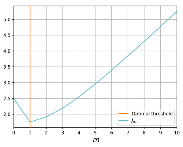
(a) Theoretical computation $J_{\pi_{m}}$.

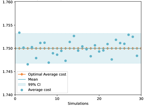
(b) Discrete event simulation.

Figure 4: For $p=0.5$, $q=0.5$, and $\kappa=10$.

Figure 5 presents the results for $p=0.4,$ $q=0.8$ and $\kappa=5$. In Figure 5(a), the optimal threshold is $m=2$. In contrast to Figure 4(a), $J_{\pi_{m}}$ appears to be “insensitive” as $m$ increases above the optimal threshold. Since platoons arrive with a high probability relative to cars, and because it is optimal to dispatch a car with an arriving platoon (according to Lemma 3.1), we expect the queue of waiting trucks to be very small. So, most of the time, the queue size does not exceed the threshold. In Figure 5(a), the mean and optimal average costs again overlap.

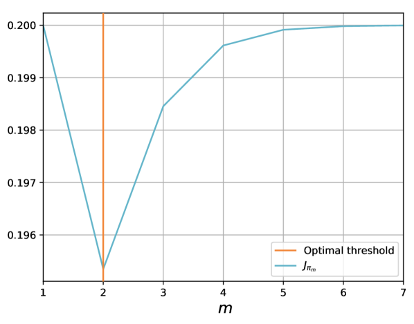
(a) Theoretical computation $J_{\pi_{m}}$.

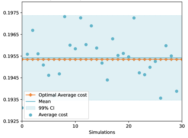
(b) Discrete event simulation.

Figure 5: For $p=0.4$, $q=0.8$, and $\kappa=5$.

In Figure 6, we present the results for $p=0.45,$ $q=0.65$ and $\kappa=20$. These results are also consistent with Lemma 4.3 when $p<q$. The threshold is $m=4$ from Figure 6(a). The mean of DES costs and the optimal average cost again overlap each other in Figure 6(b).

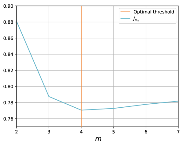
(a) Theoretical computation $J_{\pi_{m}}$.

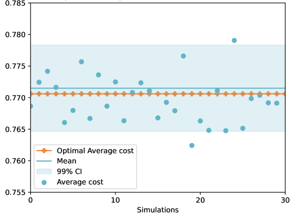
(b) Discrete event simulation.

Figure 6: For $p=0.45$, $q=0.65$, and $\kappa=20$.

6 Conclusion and Future Research

In this paper, we studied the problem of dispatching trucks to platoons arriving at a highway station. We modelled the problem as a Markov Decision Problem (with a one-dimensional Markov Chain). The dispatching action aims to minimize a cost function at the station. This function can be $\beta$-discounted (with finite or infinite horizon) as well as long-run average. We first proved that for all cost types, the optimal policy is a threshold-type policy. This threshold is finite for the finite horizon discounted cost, average cost criteria, and for the infinite horizon discounted cost when $\beta$ is sufficiently close to $1$. We then presented some numerical results regarding the optimal policy.

The results can be generalized in several ways in future work. For instance, we could consider investigating a batch dispatching model where we empty the queue upon a platoon’s arrival. More generally, we could send $r$ trucks from the station or empty it when $r\geq x_{n}$. In both models, the cost of platooning could be introduced since we assume no cost for platooning in the current model. We suspect that the optimal policy for the batch dispatching model is also of threshold type. Perhaps with a greater threshold than the current model for the same parameters since we can now send multiple trucks from the queue.

Another approach would be to investigate a model where dispatching a truck to a platoon may have random savings or costs. Finally, we could consider a model where we can dispatch $r_{n}$ trucks from the station, where $r_{n}$ will depend on the available space on an arriving platoon.

References

- Adler et al. (2020) A. Adler, D. Miculescu, and S. Karaman. Optimal Policies for Platooning and Ride Sharing in Autonomy-Enabled Transportation, pages 848–863. Springer International Publishing, Cham, 2020. ISBN 978-3-030-43089-4. doi:10.1007/978-3-030-43089-4_54. URL https://doi.org/10.1007/978-3-030-43089-4_54.
- Zabat (1995) Michael Zabat. The aerodynamic performance of platoons: Final report. PATH research report, 1995.
- Vohra et al. (2018) V. Vohra, M. Wahba, G. Akarslan, R. Ni, and S. Brennan. An examination of vehicle spacing to reduce aerodynamic drag in truck platoons. In 2018 IEEE Vehicle Power and Propulsion Conference (VPPC), pages 1–6, 2018. doi:10.1109/VPPC.2018.8604977.
- Tsugawa et al. (2016) S. Tsugawa, S. Jeschke, and S. E. Shladover. A review of truck platooning projects for energy savings. IEEE Transactions on Intelligent Vehicles, 1(1):68–77, 2016. doi:10.1109/TIV.2016.2577499.
- Hu et al. (2020) J. Hu, P. Bhowmick, F. Arvin, A. Lanzon, and B. Lennox. Cooperative control of heterogeneous connected vehicle platoons: An adaptive leader-following approach. IEEE Robotics and Automation Letters, 5(2):977–984, 2020. doi:10.1109/LRA.2020.2966412.
- Milanes et al. (2014) V. Milanes, S. E. Shladover, J. Spring, C. Nowakowski, H. Kawazoe, and M. Nakamura. Cooperative adaptive cruise control in real traffic situations. IEEE Transactions on Intelligent Transportation Systems, 15(1):296–305, 2014. doi:10.1109/TITS.2013.2278494.
- Wang et al. (2021) B. Wang, J. Zheng, Q. Ren, Y. Wu, and C. Li. Analysis of the intra-platoon message delivery delay in a platoon of vehicles. IEEE Transactions on Vehicular Technology, 70(7):7012–7026, 2021. doi:10.1109/TVT.2021.3076157.
- Petrillo et al. (2021) A. Petrillo, A. Pescape, and S. Santini. A secure adaptive control for cooperative driving of autonomous connected vehicles in the presence of heterogeneous communication delays and cyberattacks. IEEE Transactions on Cybernetics, 51(3):1134–1149, 2021. doi:10.1109/TCYB.2019.2962601.
- Zhang et al. (2017) W. Zhang, E. Jenelius, and X. Ma. Freight transport platoon coordination and departure time scheduling under travel time uncertainty. Transportation Research Part E: Logistics and Transportation Review, 98:1–23, 2017. ISSN 1366-5545. doi:https://doi.org/10.1016/j.tre.2016.11.008. URL https://www.sciencedirect.com/science/article/pii/S1366554516304938.
- A. Johansson et al. (2020) V. Turri A. Johansson, K. H. Johansson E. Nekouei, and J. Mårtensson. Truck platoon formation at hubs: An optimal release time rule. IFAC-PapersOnLine, 53(2):15312–15318, 2020. ISSN 2405-8963. doi:https://doi.org/10.1016/j.ifacol.2020.12.2338. URL https://www.sciencedirect.com/science/article/pii/S240589632033007X. 21st IFAC World Congress.
- Lippman (1973) S. A. Lippman. Semi-markov decision processes with unbounded rewards. Management Science, 19(7):717–731, 1973. ISSN 00251909, 15265501. URL http://www.jstor.org/stable/2629409.
- Viniotis and Ephremides (1987) I. Viniotis and A. Ephremides. Optimal switching of voice and data at a network node. In 26th IEEE Conference on Decision and Control, volume 26, pages 1504–1507, 1987. doi:10.1109/CDC.1987.272667.
- Lippman (1975) S. A. Lippman. Applying a new device in the optimization of exponential queuing systems. Operations Research, 23(4):687–710, 1975. ISSN 0030364X, 15265463. URL http://www.jstor.org/stable/169851.
- Lin and Kumar (1984) Woei Lin and P. Kumar. Optimal control of a queueing system with two heterogeneous servers. IEEE Transactions on Automatic Control, 29(8):696–703, 1984. doi:10.1109/TAC.1984.1103637.